Background Modeling for Double Higgs Boson Production: Density Ratios and Optimal Transport

Abstract

We study the problem of data-driven background estimation, arising in the search of physics signals predicted by the Standard Model at the Large Hadron Collider. Our work is motivated by the search for the production of pairs of Higgs bosons decaying into four bottom quarks. A number of other physical processes, known as background, also share the same final state. The data arising in this problem is therefore a mixture of unlabeled background and signal events, and the primary aim of the analysis is to determine whether the proportion of unlabeled signal events is nonzero. A challenging but necessary first step is to estimate the distribution of background events. Past work in this area has determined regions of the space of collider events where signal is unlikely to appear, and where the background distribution is therefore identifiable. The background distribution can be estimated in these regions, and extrapolated into the region of primary interest using transfer learning with a multivariate classifier. We build upon this existing approach in two ways. First, we revisit this method by developing a powerful new classifier architecture tailored to collider data. Second, we develop a new method for background estimation, based on the optimal transport problem, which relies on modeling assumptions distinct from earlier work. These two methods can serve as cross-checks for each other in particle physics analyses, due to the complementarity of their underlying assumptions. We compare their performance on simulated double Higgs boson data.

, , , , and

1 Introduction

The Standard Model (SM) of particle physics is a theory describing the interactions between elementary particles—the building blocks of matter. One key component of the SM is the presumed existence of a quantum field responsible for generating mass in certain elementary particles. This field is known as the Higgs field, originally theorized by Higgs (1964), Englert and Brout (1964). Excitations of the Higgs field produce particles, known as Higgs bosons, which were the subject of an intensive search by experimental particle physicists ever since the mid 1970s. In July 2012, two independent experiments at the Large Hadron Collider (LHC) at CERN (the European Organization for Nuclear Research) announced the observation of a new particle consistent with the SM Higgs boson (ATLAS, 2012; CMS, 2012). Having discovered this Higgs-like particle, current work is concerned with detailed studies of its properties, in order to confirm or refute those predicted by the SM. One such property is the so-called Higgs boson self-coupling, whereby a single excitation of the Higgs field can split into two Higgs bosons without intermediate interactions with other particles. Observing this phenomenon would provide compelling new information regarding the mechanism of particle mass generation. This paper is concerned with some of the statistical challenges posed by its search.

The LHC is housed in a massive underground tunnel in which two counter-rotating beams of protons are accelerated to nearly the speed of light. When these protons collide, new particles are formed, and their paths within particle detectors are recorded. Individual collisions are referred to as events. An event in which two Higgs bosons are generated is called a double Higgs (or di-Higgs) event. The Higgs boson is a highly unstable particle; whenever it is produced, it decays into other particles almost immediately, making di-Higgs production impossible to observe directly.

The Higgs boson most commonly decays into a pair of so-called bottom quarks ($b$-quarks). An event in which four $b$-quarks are observed is thus a candidate di-Higgs event, but could also have arisen from various other physical processes that produce four $b$-quarks. We say that a di-Higgs event in which the Higgs bosons decay into four $b$-quarks is a signal event, while any other event tagged as having four $b$-quarks is called a background event. The problem of searching for double Higgs boson production reduces to testing whether the proportion of signal events is nonzero among the observed data. As we describe in Section 3, carrying out this test is a well-understood statistical task when the distributions of both background and signal events are known. While the di-Higgs signal distribution can be approximated to sufficient accuracy with first-principles simulation, simulating the background distribution suffers from large high-order corrections which are computationally intractable (Di Micco et al., 2020). Instead, the background distribution must be estimated using observed data. This is known as the problem of data-driven background modeling, which is the main subject of this paper.

As stated, the background distribution is not a statistically identifiable quantity without further assumptions, due to the potential presence of an unknown proportion of signal in the data. Any analysis strategy must therefore make some modeling assumptions to make the background estimation problem tractable. As we discuss below, it is standard to assume that the background distribution is related in some way to the distribution of certain auxiliary events, which in turn is identifiable. An example of useful auxiliary events is those consisting of less than four observed $b$-quarks, since they are unlikely to be signal events, but are kinematically similar to the background events of interest (Bryant, 2018). Stated differently, the distribution of auxiliary events is an identifiable estimand which has undergone a distributional shift relative to the non-identifiable background distribution of interest. If the analyst has access to a sample of auxiliary events, its empirical distribution provides a first naive approximation of the desired background distribution. To obtain a more precise estimate, one must correct for the distributional shift.

As we discuss in Section 1.2, the most widely-used method for correcting this distributional shift is based on an estimate of the density ratio between the background and auxiliary events. This method typically first estimates the density ratio in a signal-free region of the phase space, known as the Control Region, and then extrapolates it to the region of primary interest, known as the Signal Region. Any deviation of this extrapolated density ratio from unity is used to correct the distributional shift undergone by the auxiliary sample. This extrapolation can be viewed as an instance of transfer learning (Weiss, Khoshgoftaar and Wang, 2016). While a careful choice of the density ratio estimator can greatly improve the accuracy of this extrapolation, it clearly cannot lead to a consistent estimator if the distribution in the Signal Region is unconstrained relative to its counterpart in the Control Region. This procedure thus places an implicit modeling assumption on the underlying distributions, which is challenging to quantify and verify in practice. Nevertheless, variants of this procedure have been used in each of the most recent di-Higgs searches in the four $b$-quark final state (e.g. ATLAS (2018a), ATLAS (2019a), ATLAS (2021), CMS (2022), ATLAS (2022)). This raises the important need for cross-checking the modeling assumption made by such an approach.

1.1 Our Contributions

This paper develops a new methodology for data-driven background modeling in di-Higgs boson searches. Our approach is fully nonparametric, and does not involve the extrapolation of density ratios. It hinges upon a characteristic modeling assumption, which is complementary to that of the density ratio method. These two distinct methods can thus serve as cross-checks for each other in di-Higgs searches, an important benefit that will increase the analyst’s trust in the obtained background estimates.

Our approach is based on the optimal transport problem (Villani, 2003) between multidimensional distributions of collider events. Optimal transport has already proven to be a powerful tool for transfer learning in classification problems (Courty et al., 2016), and here we propose to use it rather differently to correct distributional shifts between estimates of the auxiliary and background distributions. Our method involves out-of-sample estimation of optimal transport maps, for which we consider two different estimators. While the first is based on smoothing of an in-sample optimal coupling, and has previously been proposed in the literature (cf. Section 1.2), our second estimator appears to be new, and leverages some strengths of the density ratio approach.

The optimal transport problem requires a cost function on the space of collider events, for which we employ a variant of the metric proposed by Komiske, Metodiev and Thaler (2019). This metric is itself obtained through the optimal transport problem of matching clusters of energy deposits in collision events. Our approach therefore involves a nested use of optimal transport.

As a secondary contribution, we revisit the density ratio approach to background estimation. In particular, we recall how this approach can be reduced to fitting a probabilistic classifier for discriminating auxiliary events from background events, and we develop a powerful new classifier architecture tailored to this application. Our classifier is a convolutional neural network with residual layers (He et al., 2016), whose architecture accounts for the structure and symmetries of collider events with multiple identical final state objects.

We illustrate the empirical performance of these two methodologies on realistic simulated collider data. We observe that both approaches lead to quantitatively similar background estimates, despite the complementarity of their underlying modeling assumptions. In particular, this study illustrates how our methods can be used to cross-check each other in practice.

1.2 Related Work

Di-Higgs boson production has been the subject of numerous recent searches by the ATLAS and CMS collaborations at the LHC—we refer to the recent survey paper of Di Micco et al. (2020) for an overview. The four $b$-quark final state is the most common decay channel for di-Higgs events, but suffers from a large multijet background. As described previously, each of the most recent searches in this final state performed data-driven background estimation by first estimating a density ratio in a Control Region, and extrapolating it to the Signal Region. Certain searches, such as ATLAS (2019a), estimate the density ratio using heuristic one-dimensional reweighting schemes, while others, such as CMS (2022), use off-the-shelf multivariate classifiers for this purpose. Part of our work builds upon the latter by designing a new classifier tailored to collider data.

The idea of estimating density ratios using classifiers has a long history in statistics—see for instance Fix and Hodges (1951), Silverman and Jones (1989), Qin (1998), Cheng and Chu (2004), Kpotufe (2017)—and appears in a variety of applications in experimental particle physics (e.g., Cranmer, Pavez and Louppe (2015), Brehmer et al. (2020), CMS (2022)). Classification-based estimators have the practical advantage of circumventing the need for high-dimensional density estimation, which can be particularly challenging to perform over the space of collider events. It has been empirically observed that modern classification algorithms, such as deep neural networks, have the ability to transfer well to new distributions (Yosinski et al., 2014), which further motivates their use for density ratio estimation in our context.

Rather than density ratios, the key object of interest in our new methodology is the notion of optimal transport map. Optimal transport theory has received a surge of recent interest in the statistics and machine learning literature—we refer to Panaretos and Zemel (2019a, b); Kolouri et al. (2017); Peyré and Cuturi (2019) for recent reviews. Closest to our setting are applications of optimal transport to domain adaptation for classification problems; see for instance Courty et al. (2016), Redko, Habrard and Sebban (2017), Rakotomamonjy et al. (2022), and references therein. Nested optimal transport formulations, as in our work, have recently been used for other tasks such as multilevel clustering (Ho et al., 2017, 2019; Huynh et al., 2021) and multimodal distribution alignment (Lee et al., 2019). Very recently, optimal transport has also been used in high energy physics for calibrating stochastic simulators (Pollard and Windischhofer, 2022), for purposes of exploratory data analysis (Komiske, Metodiev and Thaler, 2019; Komiske et al., 2020; Cai et al., 2020), and for the purpose of defining a geometry on the space of collider events (Komiske, Metodiev and Thaler, 2020). We also note that optimal transport has implicitly been used for one-dimensional template morphing in the early work of Read (1999).

Our methodology relies on estimating optimal transport maps or couplings between distributions of collider events. The question of out-of-sample estimation of optimal transport maps over Euclidean spaces has been the subject of intensive recent study (Perrot et al., 2016; Forrow et al., 2018; Makkuva et al., 2019; Schiebinger et al., 2019; Nath and Jawanpuria, 2020; Hütter and Rigollet, 2021; de Lara, González-Sanz and Loubes, 2021; Deb, Ghosal and Sen, 2021; Manole et al., 2021; Pooladian and Niles-Weed, 2021; Ghosal and Sen, 2022; Gunsilius, 2022). While many of these works are tailored to the quadratic cost function, the widely-used nearest-neighbor estimator (Flamary et al., 2021; Manole et al., 2021) can naturally be defined over general metric spaces, and is used in one of our background estimators defined in Section 5.2.2.

Beyond the search of di-Higgs boson production, we emphasize that the question of data-driven background estimation arises in a variety of problems in experimental high-energy physics, where our methodologies could also potentially be applied. We refer to the book Behnke et al. (2013) for a pedagogical introduction to statistical aspects of the subject; see also Appendix 1 of Lyons (1986). Finally, we mention some recent advances on the widely-used sPlot (Barlow, 1987; Pivk and Le Diberder, 2005; Borisyak and Kazeev, 2019; Dembinski et al., 2022) and ABCD (Alison, 2015; ATLAS, 2015; Choi and Oh, 2021; Kasieczka et al., 2021) techniques for background estimation, the latter of which can be viewed as a precursor to the methods developed in this paper.

1.3 Paper Outline

The rest of this paper is organized as follows. Section 2 contains background about the LHC and di-Higgs boson production. Section 3 outlines the statistical procedure used for signal searches in collider experiments at the LHC, and mathematically formulates the data-driven background modeling problem. In Section 4, we revisit the density ratio approach to background estimation, based on classifiers for discriminating auxiliary events from background events, and we briefly describe our new classifier architecture for this purpose. In Section 5, we describe our new methodology based on the optimal transport problem. We then compare these methods in a simulated di-Higgs search in Section 6. We close with a discussion in Section 7. In the Supplementary Material, Appendix A contains a section-by-section summary of this manuscript in non-technical language, Appendices B–D contain numerical details deferred from the main text, and Appendix E contains further numerical results.

2 Background

2.1 LHC Experiments and di-Higgs Boson Production

The LHC is the largest particle collider in the world, consisting of a 27 kilometer-long tunnel in which two counter-rotating beams of protons are accelerated to nearly the speed of light. These particles are primarily collided in one of four underground detectors, named ALICE, ATLAS, CMS and LHCb. ATLAS and CMS are general-purpose detectors used for a wide range of physics analyses, including Higgs boson-related searches, while ALICE and LHCb focus on specific physics phenomena. We focus on the CMS detector in what follows, but similar descriptions can be made for the ATLAS detector.

When two protons collide, their energy is converted into matter, in the form of new particles. The goal of the CMS (Compact Muon Solenoid) detector is to measure the momenta, energies and types of such particles. To measure their momenta, CMS is built around a giant superconducting solenoid magnet, depicted in Figure 1, which deforms the trajectories of particles as they move from the center of the detector outward through a silicon tracker. The extent to which the trajectory of a charged particle is bent depends on its momentum and can hence be used to measure the momentum. After the silicon tracker, CMS consists of several layers of calorimeters which measure the energies of the particles. We refer to CMS (2008) for a complete description of the CMS detector.

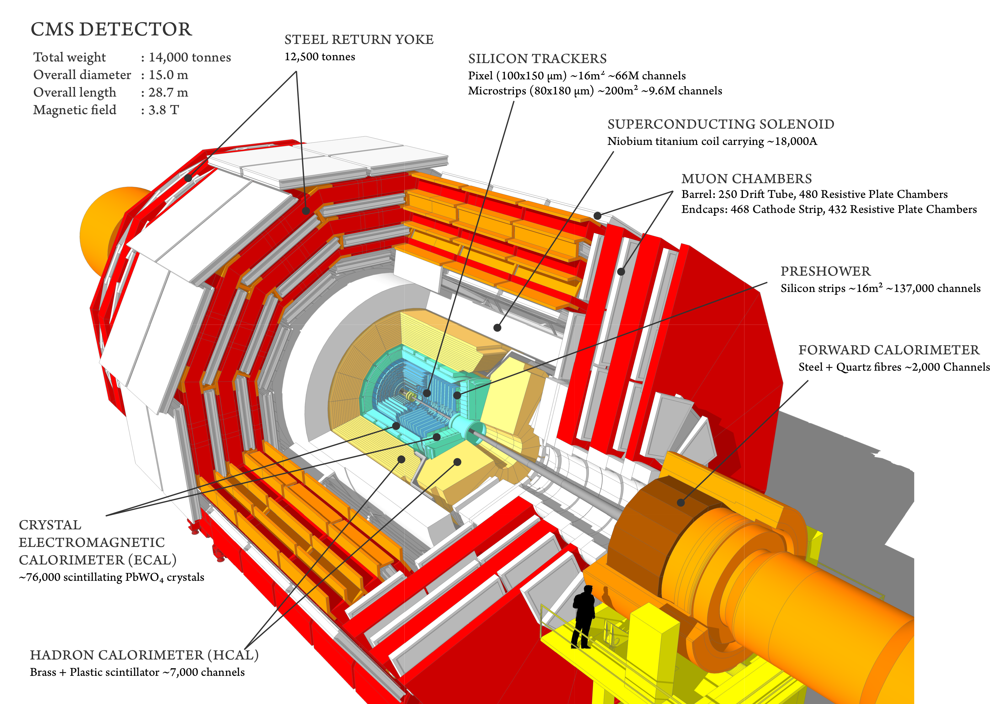
Figure 1: Illustration of the CMS detector (Sakuma and McCauley, 2014). Counter-rotating beams of protons are made to collide in the center of the detector. The trajectory and mass of each particle emanating from the collision is then recorded.

Proton-proton collisions give rise to highly unstable particles which decay almost instantly into more stable particles. The detector is only able to observe these longer-lived particles. By measuring their energies and momenta, insight can be gained into the physical properties of the unstable particles from which they originate.

The Higgs boson is an example of an unstable particle, which decays within approximately $10^{-22}$ seconds. The SM predicts that a Higgs boson decays into a pair of bottom quarks ($b$-quarks) $60\%$ of the time, and this decay channel has indeed been observed experimentally (ATLAS, 2018b; CMS, 2018a). Other channels which have been observed experimentally include the decay of a Higgs boson into pairs of photons (ATLAS, 2018c; CMS, 2018b), W bosons (ATLAS, 2018d; CMS, 2019), Z bosons (ATLAS, 2018e; CMS, 2018c), and tau leptons (ATLAS, 2019b; CMS, 2018d). The SM further predicts the rare possibility that two Higgs bosons can be produced simultaneously, and this paper is concerned with the statistical challenges arising in the search for this process, which has yet to be observed experimentally. If this process were to occur, the two resulting Higgs bosons would each, in turn, be most likely to decay into two $b$-quarks, thus making four $b$-quarks the most common final state of di-Higgs boson events. We focus on this decay channel (abbreviated HH$\rightarrow{4b}$) throughout this paper. We note that $b$-quarks form into bound states with other quarks called $b$-hadrons which are themselves unstable, and rapidly decay into collimated sprays of stable particles called $b$-jets, which can be efficiently identified by the CMS detector (CMS, 2018e).

2.2 Collider Events and the CMS Coordinate System

Particles measured by the CMS detector are typically represented in spherical coordinates. Given a particle with momentum vector $p=(x,y,z)\in\mathbb{R}^{3}$, its azimuthal angle $\phi\in[0,2\pi)$ is defined as the angle increasing from the positive $x$-axis to the positive $y$-axis, while the polar angle $\theta\in[0,\pi)$ is increasing from the positive $z$-axis to the positive $y$-axis. The length of its projection onto the $(x,y)$ plane is called the transverse momentum $p_{T}$. It is common to replace the polar angle $\theta$ by the pseudorapidity of the particle, given by $\eta=-\log(\tan(\theta/2))$.

In addition to the variables $p_{T},\eta$ and $\phi$, the rest mass $m$ of each particle can be obtained from the energy measurements made by the calorimeters in the CMS detector. Altogether, a particle jet is analyzed as a single point in this coordinate system, and encoded as a four-dimensional vector $(p_{T},\eta,\phi,m)$. In our search channel, collisions lead to multiple, say $K\geq 1$, jets measured by the detector, which may be encoded as the $4K$-dimensional vector $({p_{T}}_{i},\eta_{i},\phi_{i},m_{i}:1\leq i\leq K)$. We opt for an alternative notation, which will be particularly fruitful for the purpose of defining a metric between collider events in Section 5.3. Specifically, an event will henceforth be represented by the discrete measure

$$g=\sum_{i=1}^{K}p_{T_{i}}\delta_{(\eta_{i},\phi_{i},m_{i})},$$ (2.1)

where $\delta_{x}$ denotes the Dirac measure placing unit mass at a point $x\in\mathbb{R}^{3}$. In particular, the representation (2.1) emphasizes the invariance of an event with respect to the ordering of its jets. The transverse momenta $p_{T_{i}}$ may be viewed as a proxy for the energy of each jet, thus the total measure of $g$ denotes its total energy, denoted $s_{T}=\sum_{i=1}^{K}p_{T_{i}}$. The set of events with $K$ jets of interest is denoted by

$$\mathcal{G}^{(K)}=\left\{\sum_{j=1}^{K}p_{T_{j}}\delta_{(\eta_{j},\phi_{j},m_{j})}:p_{T_{j}},m_{j}>0,\ \phi_{j},\eta_{j}\in\mathbb{R},\ 1\leq j\leq K\right\},$$

where the definition of $\phi_{j}$ is extended from $[0,2\pi)$ to the entire real line by $2\pi$-periodicity. In the context of double Higgs boson production in the four $b$-jet final state, the choice $K=4$ will be most frequently used, and in this case we simply write $\mathcal{G}=\mathcal{G}^{(4)}$.

Finally, we note that events are deemed invariant under the orientation of the $x$- and $z$-axes. This fact, together with the periodicity of the angle $\phi$, implies that two events $g=\sum_{j=1}^{K}p_{T_{j}}\delta_{(\eta_{j},\phi_{j},m_{j})}\in\mathcal{G}^{(K)}$ and $g^{\prime}=\sum_{j=1}^{K}p_{T_{j}}^{\prime}\delta_{(\eta_{j}^{\prime},\phi_{j}^{\prime},m_{j}^{\prime})}\in\mathcal{G}^{(K)}$ may be deemed equivalent if they are mirror-symmetric in $\eta,\phi$, as well as rotationally symmetric in $\phi$, that is, if there exist $\Delta\in 2\pi\mathbb{Z}$ and $\iota_{1},\iota_{2}\in\{-1,1\}$ such that

$$\sum_{j=1}^{K}p_{T_{j}}\delta_{(\iota_{1}\eta_{j},\Delta+\iota_{2}\phi_{j},m_{j})}=\sum_{j=1}^{K}p^{\prime}_{T_{j}}\delta_{(\eta_{j}^{\prime},\phi_{j}^{\prime},m_{j}^{\prime})}.$$ (2.2)

Formally, we define an equivalence relation $\simeq$ between events in $\mathcal{G}^{(K)}$, such that $g\simeq g^{\prime}$ if and only if there exist $\Delta,\iota_{1},\iota_{2}$ for which (2.2) holds.

3 Problem Formulation

3.1 Overview of Signal Searches at the LHC

In order to make inferences about the presence or absence of a signal process in collider data, event counts are commonly analyzed as binned Poisson point processes. While we focus on the setting of double Higgs boson production in the four $b$-quark final state, the description that follows is representative of a wide range of signal searches for high-energy physics experiments.

Let $\nu_{0}$ denote a $\sigma$-finite Borel measure over the state space $\mathcal{G}$ of collider events, with respect to a fixed choice of Borel $\sigma$-algebra on $\mathcal{G}$ denoted $\mathbb{B}(\mathcal{G})$. Let $F$ denote an inhomogeneous Poisson point process (Reiss, 2012) with a nonnegative intensity function $f\in L^{2}(\mathcal{G})$ on $\mathcal{G}$, that is, $F$ is a random point measure on $\mathcal{G}$ such that

1. $F(A)\sim\text{Poisson}(\lambda(A))$, where $\lambda$ is the intensity measure induced by $f$, defined by $\lambda(A)=\int_{A}f\,\mathrm{d}\nu_{0}$ for all $A\in\mathbb{B}(\mathcal{G})$;

2. $F(A_{1}),\dots,F(A_{\ell})$ are independent for all pairwise disjoint sets $A_{1},\dots,A_{\ell}\in\mathbb{B}(\mathcal{G})$, for all integers $\ell\geq 1$.

Every four $b$-jet collision event is either a signal event, namely an event arising from two Higgs bosons, or a background event, arising from some other physical process. Letting $\mu\geq 0$ denote the rate of signal events, we write the intensity measure $\lambda$ as

$$\lambda(\cdot)=\beta_{4}(\cdot)+\mu\sigma(\cdot),$$

where $\beta_{4}$ and $\sigma$, respectively, denote nonnegative background and signal intensity measures. $\sigma$ is typically normalized such that the value $\mu=1$ corresponds to the theoretical prediction of the signal rate. The measures $\beta_{4}$ and $\sigma$ typically depend on nuisance parameters related to the calibration of the detector, the uncertain parameters of certain physical processes, such as the parton distribution functions of the proton (Placakyte, 2011), and so on. We suppress the dependence on such nuisance parameters for ease of exposition. The parameter $\mu$ is of primary interest, since non-zero values of $\mu$ indicate the existence of signal events. A search for the signal process therefore reduces to testing the following hypotheses on the basis of observations from the Poisson point process $F$:

$$H_{0}:\mu=0\quad\text{ vs. }\quad H_{1}:\mu>0.$$ (3.1)

Given a sequence $G_{1},G_{2},\dots$ of observed events, we may write $F=\sum_{i=1}^{M}\delta_{G_{i}}$, where $M\sim\text{Poisson}(\lambda(\mathcal{G}))$ is independent of the observations, which satisfy

$$G_{1},G_{2},\dots\overset{\text{iid}}{\sim}\frac{\lambda}{\lambda(\mathcal{G})}=\epsilon S+(1-\epsilon)P_{4}.$$ (3.2)

Here, $S=\sigma/\sigma(\mathcal{G})$ and $P_{4}=\beta_{4}/\beta_{4}(\mathcal{G})$ denote the respective signal and background distributions, and $\epsilon=\mu\sigma(\mathcal{G})/\lambda(\mathcal{G})$ the proportion of signal events.

The Poisson point process $F$ is often binned in practice. Let $\xi:\mathcal{G}\to\mathcal{A}\subseteq\mathbb{R}$ denote a dimensionality reduction map, to be discussed below, which will be used to bin the point process using univariate bins. Let $\{I_{j}\}_{j=1}^{J}$ denote a collection of bins forming a partition of $\mathcal{A}$, and define the event counts

$$D_{j}=F\big{(}\xi^{-1}(I_{j})\big{)}=\big{|}\{1\leq i\leq M:\xi(G_{i})\in I_{j}\}\big{|},\quad j=1,\dots,J.$$ (3.3)

The definition of $F$ implies that the random variables $D_{j}$ are independent and satisfy

$$D_{j}\sim\text{Poisson}\big{(}B_{j}+\mu S_{j}\big{)},\quad j=1,\dots,J,$$ (3.4)

where $B_{j}=\beta_{4}(\xi^{-1}(I_{j}))$ and $S_{j}=\sigma(\xi^{-1}(I_{j}))$.

The likelihood ratio test with respect to the joint distribution of $D_{1},\dots,D_{J}$ is typically used to test the hypotheses (3.1) (ATLAS, CMS and Higgs Combination Group, 2011). The binned likelihood function for the parameter $\mu$ is given by

$$L(\mu)=\prod_{j=1}^{J}\frac{\big{(}B_{j}+\mu S_{j}\big{)}^{D_{j}}}{D_{j}!}e^{-\big{(}B_{j}+\mu S_{j}\big{)}}.$$ (3.5)

Di-Higgs events are rare in comparison to background events, thus the signal-to-background ratio is low. At the time of writing, values of $M$ which are typically observed at the LHC may be too small for any test to have power in rejecting the null hypothesis in (3.1) at desired significance levels (Di Micco et al., 2020). Analyses which fail to reject $H_{0}$ instead culminate in an upper confidence bound on $\mu$, also known as an upper limit (ATLAS, CMS and Higgs Combination Group, 2011).

The power of the likelihood ratio test for (3.1) may be increased by choosing a function $\xi$ which maximizes the separation between background and signal event counts across the $J$ bins. Informally, the optimal such choice of $\xi$ is given by

$$\xi(g)=\mathbb{P}(G\text{ is a Signal Event}|G=g),$$ (3.6)

which may be estimated using a multivariate classifier, such as a neural network or boosted decision trees, for discriminating background events from signal events.

The signal intensity measure $\sigma$ is theoretically predicted by the SM, and can be approximated well using Monte Carlo event generators (Di Micco et al., 2020). The background intensity $\beta_{4}$ is, however, intractable due to the strongly interacting nature of quantum chromodynamics (QCD) in which events with the four $b$-quark final state can be produced via an enormous number of relevant and complex pathways. The intensity measure $\beta_{4}$, or its binned analogue $(B_{j})_{j=1}^{J}$, must therefore be estimated from the collider data itself, which we refer to as data-driven background modeling. This problem constitutes the primary focus of this paper.

3.2 Setup for Data-Driven Background Modeling

The aim of this paper is to develop data-driven estimators of the background intensity measure $\beta_{4}$. The primary challenge is the fact that the sample $G_{1},\dots,G_{M}$ is contaminated with an unknown proportion $\epsilon$ of signal events. The background estimation problem is thus statistically unidentifiable as stated, and it will be necessary to impose further modeling assumptions.

In order to formulate these assumptions and our resulting background modeling methods, we assume that the analyst has access to a second Poisson Point Process $T=\sum_{i=1}^{N}\delta_{H_{i}}$ consisting of auxiliary events which were tagged by the CMS detector as having four jets, of which exactly three are $b$-jets. We refer to such events as “$3b$ events”, as opposed to “$4b$ events” which were identified as having four $b$-jets. We stress that the terms $3b$ and $4b$ do not refer to the true number of $b$-quarks arising from the collision, rather the number of $b$-jets identified by the detector. As we further discuss in Section 6, the majority of $3b$ events in fact arise from the hadronization of two $b$-quarks and two charm or light quarks, while a small proportion arise from four $b$-quarks. For the purpose of a discovery analysis, the $3b$ sample $H_{1},H_{2},\dots,H_{N}$ can therefore be treated as having a negligible proportion of signal events (Bryant, 2018; CMS, 2022). We treat this proportion as zero for sake of exposition. We shall henceforth denote the intensity measure of the point process $T$ by $\beta_{3}$, and we denote by $P_{3}=\beta_{3}/\beta_{3}(\mathcal{G})$ the corresponding probability distribution of the independent observations $H_{1},H_{2},\dots$.

The kinematics of $3b$ events are similar, but not equal, to those of $4b$ background events (CMS, 2022). Unlike $\beta_{4}$, however, the intensity measure $\beta_{3}$ is an identifiable estimand due to the lack of signal events in the point process $T$. Any consistent estimator $\widehat{\beta}_{3}$ of $\beta_{3}$ can be used to provide a zeroth-order approximation of $\beta_{4}$ (up to a correction for normalization). This approximation is, however, insufficiently accurate to be used as a final estimate of $\beta_{4}$ and our goal is to develop statistical methods for correcting this naive background estimate.

Recall that the four $b$-jets of any signal event $g\in\mathcal{G}$ are naturally paired, with each pair arising from a Higgs boson. The true pairing of the jets is unknown to the detector; however, it may be approximated, for instance using an algorithm due to Bryant (2018). We use the same pairing algorithm in our work. Given as input an event $g$, this deterministic algorithm outputs one among the three distinct unordered pairs of measures $\{g^{1},g^{2}\}\subseteq\mathcal{G}^{(2)}$ which satisfy $g=g^{1}+g^{2}$. We refer to $g^{1}$ and $g^{2}$ as dijets. When $g$ is a signal event, we expect that each dijet arose from a decay of a Higgs boson, whereas when $g$ is a background event, we expect that at least one of the two dijets arose from the decay of a different particle.

The Higgs boson is known to have mass $m_{H}$ approximately equal to 125 GeV (ATLAS, 2012; CMS, 2012). It follows that the two dijets should approximately satisfy $m(g^{1})\approx m(g^{2})\approx m_{H}$, where $m(a)$ denotes the invariant mass of any $a\in\mathcal{G}^{(K)}$, $K\geq 1$. Large deviations of the dijet invariant masses from 125 GeV indicate that $g$ is not a signal event. This provides a heuristic for determining events among $G_{1},\dots,G_{M}$ which are unlikely to be signal events. To elaborate, we form subsets $\mathcal{G}_{c},\mathcal{G}_{s}\subseteq\mathcal{G}$ such that $\mathcal{G}_{c}\cap\mathcal{G}_{s}=\emptyset$, where $\mathcal{G}_{s}$ is called the Signal Region, containing events with dijet masses near $m_{H}$, and $\mathcal{G}_{c}$ is called the Control Region, containing all other events which will be used in the analysis. We follow Bryant (2018) and employ the following specific definitions of $\mathcal{G}_{c}$ and $\mathcal{G}_{s}$:

$$\mathcal{G}_{s} =\left\{g\in\mathcal{G}:\sqrt{\left(1-\frac{m_{H}}{m(g^{1})}\right)^{2}+\left(1-\frac{m_{H}}{m(g^{2})}\right)^{2}}\leq\kappa_{s}\right\},$$ (3.7)

$$\mathcal{G}_{c} =\left\{g\in\mathcal{G}:\sqrt{\Big{(}m(g^{1})-\sigma_{C}m_{H}\Big{)}^{2}+\Big{(}m(g^{2})-\sigma_{C}m_{H}\Big{)}^{2}}\leq\kappa_{c}\right\}\setminus\mathcal{G}_{s},$$ (3.8)

for some constants $\sigma_{c},\kappa_{c},\kappa_{s}>0$.

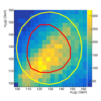
Figure 2: Illustration of the Control and Signal Regions. The two-dimensional histogram represents simulated 4b collider events described in Section 6, plotted in terms of their dijet invariant masses. We emphasize that this is a low-dimensional representation; the events considered in this work are 16-dimensional. The red line indicates the boundary of the Signal Region, while the annulus bounded by the yellow and red lines represents the Control Region. The constants $\sigma_{c},\kappa_{c}$ and $\kappa_{s}$ used in this figure are stated in Section 6.

These regions are illustrated in Figure 2. We similarly partition the Poisson intensity measures $\beta_{3},\beta_{4}$, by defining for all $A\in\mathbb{B}(\mathcal{G})$,

$$\beta_{j}^{c}(A)=\beta_{j}(A\cap\mathcal{G}_{c}),\quad\beta_{j}^{s}(A)=\beta_{j}(A\cap\mathcal{G}_{s}),\quad j=3,4.$$

These four measures are illustrated in Figure 3. Furthermore, we assume for ease of exposition that these measures are absolutely continuous with respect to the dominating measure $\nu_{0}$, and we let $b_{j}^{a}=d\beta_{j}^{a}/d\nu_{0}$ for all $j=3,4$ and $a=c,s$.

Recall that the collider events associated with the intensity measures $\beta_{3}^{c}$ and $\beta_{3}^{s}$ are signal-free by construction, and those from $\beta_{4}^{c}$ are also signal-free under the assumption that negligibly few signal events will fall outside of $\mathcal{G}_{s}$. These three intensity measures can therefore be estimated directly by means of their empirical intensity functions. We have thus reduced the background modeling problem to that of estimating $\beta_{4}^{s}$, given estimates of $\beta_{3}^{c}$, $\beta_{3}^{s}$ and $\beta_{4}^{c}$.

To this end, we will partition the samples into the sets

$$\{G_{1}^{s},\dots,G_{m_{s}}^{s}\} :=\{G_{1},\dots,G_{M}\}\cap\mathcal{G}_{s},\qquad \{H_{1}^{s},\dots,H_{n_{s}}^{s}\} :=\{H_{1},\dots,H_{N}\}\cap\mathcal{G}_{s},$$

$$\{G_{1}^{c},\dots,G_{m_{c}}^{c}\} :=\{G_{1},\dots,G_{M}\}\cap\mathcal{G}_{c},\qquad \{H_{1}^{c},\dots,H_{n_{c}}^{c}\} :=\{H_{1},\dots,H_{N}\}\cap\mathcal{G}_{c},$$

where $M=m_{c}+m_{s}$ and $N=n_{c}+n_{s}$. Furthermore, let

$$\beta^{c}_{3,n_{c}}=T|_{\mathcal{G}_{c}}=\sum_{i=1}^{n_{c}}\delta_{H_{i}^{c}},\quad\beta^{s}_{3,n_{s}}=T|_{\mathcal{G}_{s}}=\sum_{i=1}^{n_{s}}\delta_{H_{i}^{s}},\quad\beta^{c}_{4,m_{c}}=F|_{\mathcal{G}_{c}}=\sum_{i=1}^{m_{c}}\delta_{G_{i}^{c}}$$

denote the empirical estimators of the measures $\beta_{3}^{c},\beta_{3}^{s},\beta_{4}^{c}$, illustrated in the background of Figure 3. As previously noted, the measure $\beta_{3}^{s}$ provides a zeroth-order approximation of $\beta_{4}^{s}$ (after a normalization correction), thus a naive first estimate of $\beta_{4}^{s}$ is given by $\beta^{s}_{3,n_{s}}$. As we shall see in the simulation study of Section 6, this approximation is insufficiently accurate to be used as a final estimator. Our methodologies improve upon it by modeling the discrepancy between the $3b$ and $4b$ distributions in the Control Region via $\beta_{4,m_{c}}^{c},\beta_{3,n_{c}}^{c}$, and then making use of that information in the Signal Region to improve the accuracy of $\beta^{s}_{3,n_{s}}$ as an estimator of $\beta_{4}^{s}$.

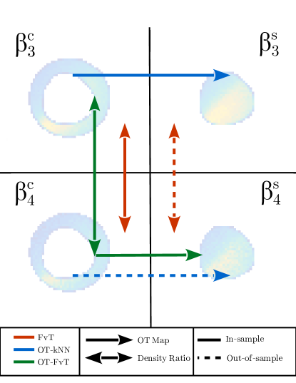
Figure 3: Illustration of the four Poisson intensity measures $\beta_{3}^{c},\beta_{3}^{s},\beta_{4}^{c},\beta_{4}^{s}$, among which only the latter is nontrivial to estimate, and summary of the three methods developed in this paper for estimating $\beta_{4}^{s}$. The method FvT (Four vs. Three) estimates the ratio of the two densities in the Control Region using a classifier, and then extrapolates it into the Signal Region using out-of-sample evaluations of the classifier. The OT-$k$NN (Optimal Transport–$k$ Nearest Neighbors) method produces an estimator $\widehat{T}$ of the optimal transport map $T$ between the $3b$ Control and Signal Region distributions, and evaluates this estimator out-of-sample on an estimator of the 4b Control Region distribution. The out-of-sample evaluation of $\widehat{T}$ is performed using nearest-neighbor extrapolation. The OT-FvT (Optimal Transport–Four vs. Three) method combines these ideas: first, it uses the classifier to produce an estimator of $\beta_{4}^{c}$ with the same support as $\beta_{3,n_{c}}^{c}$, and second, it pushes forward this estimator through $\widehat{T}$, thereby avoiding out-of-sample evaluations of both the classifier and optimal transport map. The background of the figure consists of bivariate histograms of simulated $3b$ and $4b$ samples in the Control and Signal Regions, plotted in terms of their dijet invariant masses, as in Figure 2.

Once we are able to derive an estimator $\widehat{\beta}_{4}^{s}$ of $\beta_{4}^{s}$, based on the signal-free observations $G_{1}^{c},\dots,G_{m_{c}}^{c},$ $H_{1}^{s},\dots,H_{n_{s}}$, $H_{1}^{c},\dots,H_{n_{c}}^{c}$, we may define the fitted histogram $\widehat{B}_{j}=\widehat{\beta}_{4}^{s}(\xi^{-1}(I_{j}))$, $j=1,\dots,J$. One may then test the hypotheses (3.1) using the likelihood ratio test, based on the following modification of the likelihood function in equation (3.5),

$$\widetilde{L}(\mu)=\prod_{J=1}^{J}\frac{\left(\widehat{B}_{j}+\mu S_{j}\right)^{D_{j}^{s}}}{D_{j}^{s}!}e^{-\left(\widehat{B}_{j}+\mu S_{j}\right)},\quad\text{where }D_{j}^{s}=\left|\left\{1\leq i\leq m_{s}:\xi(G_{i}^{s})\in I_{j}\right\}\right|.$$ (3.9)

Here, $\widetilde{L}$ can be viewed as a restriction of the likelihood $L$ to the Signal Region. Notice that $\widehat{B}_{j}$ is independent of $D_{k}^{s}$, for any $j,k$. In practice, it is also necessary to incorporate statistical and systematic uncertainties pertaining to the estimator $\widehat{B}_{j}$ into the hypothesis testing procedure (ATLAS, CMS and Higgs Combination Group, 2011). Since formal uncertainty quantification for background modeling is beyond the scope of this work, we omit further details, and provide further discussion of this point in Section 7.

The primary difficulty remaining in the testing problem (3.1) is that of deriving estimators of the background intensity measure $\beta_{4}^{s}$. In what follows, we describe two classes of estimators for $\beta_{4}^{s}$: one based on density ratio estimation (Section 4), and the second based on optimal transport (Section 5). The former is the most common approach to di-Higgs background modeling, and will later be referred to as the FvT method. The latter is new, and we will discuss two different instances of this approach, which will later be referred to as the OT-$k$NN and OT-FvT methods. These three distinct estimators are summarized in Figure 3.

4 Background Modeling via Density Ratio Extrapolation

The discrepancy between $3b$ and $4b$ background distributions may be directly quantified in the Control Region, where no signal events are present. Under a suitable modeling assumption, this discrepancy may be extrapolated into the Signal Region to produce a correction of the $3b$ signal region intensity measure $\beta_{3}^{s}$, leading to an estimate of $\beta_{4}^{s}$. This general strategy forms the basis of most background modeling methodologies used in recent di-Higgs searches, as discussed in Section 1. The aim of this section is to recall how this approach may be carried out using a classifier for discriminating $3b$ and $4b$ events. We then briefly describe a new classifier architecture specifically tailored to this type of collider data, which will be used in our numerical studies.

Let $E$ denote a random collider event, arising from either the $3b$ or $4b$ distributions, and define the latent binary random variable $Z$ indicating the component membership of $E$. More specifically, let $Z$ be a Bernoulli random variable with success probability $\mathbb{P}(Z=1)=\beta_{4}(\mathcal{G})/(\beta_{4}(\mathcal{G})+\beta_{3}(\mathcal{G}))$, and let $E$ be generated according to the mixture model

$$E|Z=0\sim P_{3},\quad E|Z=1\sim P_{4}.$$

Setting $\psi(g)=\mathbb{P}(Z=1|E=g)$ for all $g\in\mathcal{G}$, it follows from Bayes’ Rule that

$$\frac{b_{4}^{c}(g)}{b_{3}^{c}(g)}=\frac{\psi(g)}{1-\psi(g)},\quad g\in\mathcal{G}_{c},$$ (4.1)

where we recall that $b_{j}^{c}$ denotes the intensity function associated to $\beta_{j}^{c}$, $j=3,4$. Therefore,

$$\beta_{4}^{c}(A)=\int_{A}\frac{\psi(g)}{1-\psi(g)}\,\mathrm{d}\beta_{3}^{c}(g),\quad A\in\mathbb{B}(\mathcal{G}_{c}).$$ (4.2)

Equations (4.1–4.2) are a reformulation for our context of the well-known fact that, up to normalization, a likelihood ratio may be expressed as an odds ratio (Silverman and Jones, 1989). Estimating the ratio of $3b$ to $4b$ intensity functions in the Control Region thus reduces to the classification problem of estimating $\psi$, say by a classifier $\widehat{\psi}$. This observation has the practical advantage of circumventing the need of performing high-dimensional density estimation. Assuming that the estimator $\widehat{\psi}$ can be evaluated in the Signal Region $\mathcal{G}_{s}$, disjoint from its training region $\mathcal{G}_{c}$, we may postulate that the measure

$$A\in\mathbb{B}(\mathcal{G}_{s})\longmapsto\int_{A}\frac{\widehat{\psi}(g)}{1-\widehat{\psi}(g)}\,\mathrm{d}\beta_{3}^{s}(g)$$ (4.3)

provides a reasonable approximation of $\beta_{4}^{s}$. The quality of such an approximation is driven by the ability of the classifier $\widehat{\psi}$ to generalize between regions of the phase space. To formalize this, we will assume for simplicity that $\widehat{\psi}$ is an empirical risk minimizer taking values in a class $\{\psi_{\alpha}:\mathcal{G}\to[0,1]:\alpha\in\Omega\}$, for some parameter space $\Omega\subseteq\mathbb{R}^{d}$, $d\geq 1$. That is, we assume

$$\widehat{\psi}=\psi_{\widehat{\alpha}},~{}~{}\text{where}~{}~{}\widehat{\alpha}=\operatorname*{argmin}_{\alpha\in\Omega}\left\{\frac{1}{n_{c}}\sum_{i=1}^{n_{c}}\mathcal{L}\big{(}\psi_{\alpha}(H_{i}^{c}),0\big{)}+\frac{1}{m_{c}}\sum_{j=1}^{m_{c}}\mathcal{L}\big{(}\psi_{\alpha}(G_{j}^{c}),1\big{)}\right\},$$

for some loss function $\mathcal{L}:[0,1]\times[0,1]\to\mathbb{R}$. We then make the following assumption:

Assumption 1.

The conditional probability $\psi$ satisfies the following conditions:

• (Correct Specification) There exists $\alpha^{*}\in\Omega$ such that $\psi=\psi_{\alpha^{*}}$.

• (Generalization) We have

  $$\alpha^{*}=\operatorname*{argmin}\limits_{\alpha\in\Omega}\mathbb{E}\big{[}\mathcal{L}(\psi_{\alpha}(G),Z)|G\in\mathcal{G}_{c}\big{]}.$$

Assumption 1 implies that a classifier trained solely in the Control Region can consistently estimate the full conditional probability $\psi(g)$, for events $g\in\mathcal{G}$ lying in both the Control and Signal Regions. Such an assumption guarantees the ability of the classifier $\widehat{\psi}$ to generalize from the Control Region, making the ansatz (4.3) justified. A natural estimator for $\beta_{4}^{s}$ is then obtained by replacing $\beta_{3}^{s}$ in equation (4.3) by its empirical counterpart $\beta_{3,n_{s}}^{s}$. Doing so leads to the estimator

$$\widehat{\beta}^{s}_{4}=\sum_{i=1}^{n_{s}}\frac{\widehat{\psi}(H_{i}^{s})}{1-\widehat{\psi}(H_{i}^{s})}\delta_{H_{i}^{s}}.$$ (4.4)

$\widehat{\beta}^{s}_{4}$ is called the FvT estimator, and we refer to $\widehat{\psi}$ as the FvT (Four vs. Three) classifier.

The validity of Assumption 1 relies crucially upon the choice of the function class $\{\psi_{\alpha}\}$, or equivalently the choice of the classifier $\widehat{\psi}$. Indeed, off-the-shelf classifiers may lack the generalization ability to satisfy Assumption 1(ii). A secondary contribution of our work is to propose a new classifier architecture specifically tailored to four-jet collider events, which we now briefly describe.

The FvT Classifier. Our aim is to design a classifier $\widehat{\psi}$ over $\mathcal{G}$, which

1. is invariant to the ordering of the constituent jets in an input event $g$;

2. is invariant with respect to the equivalence relation $\simeq$ defined in (2.2);

3. incorporates the dijet substructure of an event $g=g^{1}+g^{2}$.

In Appendix B, we describe how these properties can be satisfied using a customized convolutional neural network architecture with residual layers, or ResNet (He et al., 2016). We refer to the resulting classifier as the FvT classifier, and implement the FvT method with this choice throughout our numerical studies in Section 6. Beyond its use for background modeling, we also employ this classifier for the final dimensionality reduction map $\xi$ in equation (3.6). Choosing these two classifiers to have the same architecture is important in practice, since a classifier capable of learning the relevant features for signal extraction should also be capable of learning and then correcting those same features in the background model.

5 Background Modeling via Optimal Transport

The methodology described in the previous section hinged upon the ability of the classifier $\widehat{\psi}$ to accurately extrapolate from the Control Region to the Signal Region, implying that the $3b$ and $4b$ intensity functions in the latter region are constrained by their values in the former region. The validity of this assumption is difficult to verify in practice due to the blinding of the $4b$ signal region which motivates us to develop a distinct approach with a complementary modeling assumption. In this section, rather than extrapolating the discrepancy between the $3b$ and $4b$ intensity functions, we will extrapolate the discrepancy between the Control and Signal Region intensity functions, as illustrated in Figure 3.

We cannot use a density ratio to quantify the discrepancy between the intensity functions in the Control and Signal Regions, because these regions are disjoint. We will instead use the notion of a transport map, which will be defined below. In order to employ transport maps, it will be convenient to normalize all intensity functions throughout this section. That is, we will define an estimator for $\beta_{4}^{s}$ by separately estimating the probability measure $P_{4}^{s}=\beta_{4}^{s}/\beta_{4}^{s}(\mathcal{G}_{s})$ and the normalization $\beta_{4}^{s}(\mathcal{G}_{s})$. More generally, we write

$$P_{j}^{c}=\beta_{j}^{c}/\beta_{j}^{c}(\mathcal{G}_{c}),\quad P_{j}^{s}=\beta_{j}^{s}/\beta_{j}^{s}(\mathcal{G}_{s}),\quad j=3,4,$$

to denote the four population-level probability measures, with corresponding empirical measures

$$P_{3,n_{a}}^{a}=\frac{1}{n_{a}}\sum_{i=1}^{n_{a}}\delta_{H_{i}^{a}},\quad P_{4,m_{a}}^{a}=\frac{1}{m_{a}}\sum_{i=1}^{m_{a}}\delta_{G_{i}^{a}},\quad a\in\{c,s\}.$$

A transport map (Villani, 2003) between $P_{3}^{c}$ and $P_{3}^{s}$ is any Borel-measurable function $T:\mathcal{G}_{c}\to\mathcal{G}_{s}$ such that whenever $H\sim P_{3}^{c}$, we have $T(H)\sim P_{3}^{s}$. When this condition holds, we write $P_{3}^{s}=T_{\#}P_{3}^{c}$, and we say $T$ pushes $P_{3}^{c}$ forward onto $P_{3}^{s}$, or that $P_{3}^{s}$ is the pushforward of $P_{3}^{c}$ under $T$. Equivalently, this condition holds if and only if

$$P_{3}^{s}(A)=T_{\#}P_{3}^{c}(A)=P_{3}^{c}(T^{-1}(A)),\quad\text{for all }A\in\mathbb{B}(\mathcal{G}_{s}).$$

We propose to perform background estimation under the following informal modeling assumption, which will be stated more formally in the sequel.

Assumption 2’.

There exists a map $T_{0}:\mathcal{G}_{c}\to\mathcal{G}_{s}$ such that

$${T_{0}}_{\#}P_{3}^{c}=P_{3}^{s},\quad\text{and}\quad{T_{0}}_{\#}P_{4}^{c}=P_{4}^{s}.$$ (5.1)

Assumption 2’ requires the $3b$ and $4b$ distributions to be sufficiently similar for there to exist a shared map $T_{0}$ which pushes forward their restrictions to the Control Region into their counterparts in the Signal Region. If such a map $T_{0}$ were available, it would suggest the following procedure for estimating $P_{4}^{s}$:

1. Fit an estimator $\widehat{T}$ of $T_{0}$ based only on the $3b$ observations;

2. Given any estimator $\widehat{P}_{4,m_{c}}^{c}$ of $P_{4}^{c}$, use the pushforward $\widehat{T}_{\#}\widehat{P}_{4,m_{c}}^{c}$ as an estimator of $P_{4}^{s}$.

For this approach to be practical, we must specify an explicit candidate $T_{0}$ satisfying Assumption 2’. We propose to choose $T_{0}$ such that its movement of the probability mass from $P_{3}^{c}$ into that of $P_{3}^{s}$ is minimal. This leads us to consider the classical optimal transport problem, which we now describe.

5.1 The Optimal Transport Problem

Assume a metric $W$ on the space $\mathcal{G}$ is given; we provide a candidate for such a metric in Section 5.3. For any transport map $T$ pushing $P_{3}^{c}$ forward onto $P_{3}^{s}$, we refer to $W(h,T(h))$ as the cost of moving an event $h\in\mathcal{G}_{c}$ to an event $T(h)\in\mathcal{G}_{s}$. The optimal transport problem seeks to find the choice of $T$ which minimizes the expected cost of transporting $P_{3}^{c}$ onto $P_{3}^{s}$, which amounts to solving the following optimization problem

$$\operatorname*{argmin}_{T:\mathcal{G}_{c}\to\mathcal{G}_{s}}\int_{\mathcal{G}_{c}}W(h,T(h))\,\mathrm{d}P_{3}^{c}(h),\quad\text{s.t. }T_{\#}P_{3}^{c}=P_{3}^{s}.$$ (5.2)

Equation (5.2) is known as the Monge problem (Monge, 1781). When a solution $T_{0}$ to the Monge problem exists, it is said to be an optimal transport map. We postulate that, when it exists, the optimal transport map from $P_{3}^{c}$ to $P_{3}^{s}$ is a sensible candidate for the map $T_{0}$ appearing in the statement of Assumption 2’.

A shortcoming of this choice is the requirement that there exist a solution to the optimization problem (5.2). It is well-known that the Monge problem over Euclidean space admits a unique solution for absolutely continuous distributions, when the cost function is the squared Euclidean norm (Knott and Smith, 1984; Brenier, 1991). While sufficient conditions for the solvability of the Monge problem in more general spaces are given by Villani (2008, Chapter 9), we do not know whether they are satisfied by the metric space $(\mathcal{G},W)$ under consideration. Furthermore, the Monge problem may not even be feasible between distributions which are not absolutely continuous, which precludes the possibility of estimating $T_{0}$ using the optimal transport map between the empirical measures of $P_{3}^{c}$ and $P_{3}^{s}$.

Motivated by these considerations, we introduce a classical relaxation of the Monge problem, known as the Kantorovich optimal transport problem (Kantorovich, 1942, 1948). Let $\Pi(P_{3}^{c},P_{3}^{s})$ denote the set of all joint Borel distributions $\pi$ over $\mathcal{G}_{c}\times\mathcal{G}_{s}$ whose marginals are, respectively, $P_{c}^{3}$ and $P_{s}^{3}$, in the sense that $P_{3}^{c}(\cdot)=\pi(\cdot\times\mathcal{G}_{s})$ and $P_{3}^{s}(\cdot)=\pi(\mathcal{G}_{c}\times\cdot)$. We refer to such joint distributions as couplings. Consider the minimization problem

$$\mathcal{W}(P_{3}^{c},P_{3}^{s})=\inf_{\pi\in\Pi(P_{3}^{c},P_{3}^{s})}\int_{\mathcal{G}_{c}\times\mathcal{G}_{s}}W(g,h)\,\mathrm{d}\pi(g,h).$$ (5.3)

When the infimum in (5.3) is achieved by a coupling $\pi_{0}$, this last is known as an optimal coupling. When an optimal coupling is supported on a set of the form $\{(h,T(h)):h\in\mathcal{G}_{c}\}$, for some map $T:\mathcal{G}_{c}\to\mathcal{G}_{s}$, it can be seen that $T$ is in fact an optimal transport map between $P_{3}^{c}$ and $P_{3}^{s}$. The Kantorovich problem (5.3) is therefore a relaxation of the Monge problem (5.2). Unlike the latter, however, the minimization problem (5.3) is always feasible since $\Pi(P_{3}^{c},P_{3}^{s})$ is non-empty; indeed, $\Pi(P_{3}^{c},P_{3}^{s})$ always contains the independence coupling $P_{3}^{c}\otimes P_{3}^{s}$. Moreover, the infimum in the Kantorovich problem is achieved as long as the cost function $W$ is lower semi-continuous, and the measures $P_{3}^{c}$ and $P_{3}^{s}$ satisfy a mild moment condition (Villani (2008), Theorem 4.1). We also note that the optimal objective value $\mathcal{W}(P_{3}^{c},P_{3}^{s})$ defines a metric between probability measures called the (first-order) Wasserstein distance (Villani, 2003), or Earth Mover’s distance (Rubner, Tomasi and Guibas, 2000).

Using the Kantorovich relaxation, we now formalize Assumption 2’ into the following condition, which we shall require throughout the remainder of this section.

Assumption 2.

Assume there exists an optimal coupling $\pi_{0}\in\Pi(P_{3}^{c},P_{3}^{s})$ between $P_{3}^{c}$ and $P_{3}^{s}$. Given a pair of random variables $(H^{c},H^{s})\sim\pi_{0}$, let $\pi_{0}(\cdot|h)$ denote the conditional distribution of $H^{s}$ given $H^{c}=h$, for any $h\in\mathcal{G}_{c}$. Then, the following implication holds:

$$\begin{aligned} G^{c}&\sim P_{4}^{c}\\[-3.61371pt] G^{s}|G^{c}&\sim\pi_{0}(\cdot|G^{c})\end{aligned}~{}~{}\Longrightarrow~{}~{}G^{s}\sim P_{4}^{s}.$$ (5.4)

Assumption 2 requires the $3b$ and $4b$ distributions to be sufficiently similar for their restrictions to the Signal and Control Regions to be related by a common conditional distribution. It further postulates that this conditional distribution is induced by the optimal coupling $\pi_{0}$. Heuristically, $\pi_{0}(\cdot|H)$ plays the role of a multivalued optimal transport map for pushing an event $H$ from the distribution $P_{3}^{c}$ onto $P_{3}^{s}$. Assumption 2 requires this map to additionally push the distribution $P_{4}^{c}$ onto its counterpart $P_{4}^{s}$ in the Signal Region. In the special case where there exists an optimal transport map $T_{0}$ from $P_{3}^{c}$ to $P_{3}^{s}$, we note that $\pi_{0}=(Id,T_{0})_{\#}P_{3}^{c}$ is an optimal coupling of $P_{3}^{c}$ with $P_{3}^{s}$, where $Id$ denotes the identity map. In this case, equation (5.4) is tantamount to equation (5.1).

5.2 Background Estimation

We next derive estimators for the background distribution $P_{4}^{s}$ under Assumption 2. It follows from equation (5.4) and the law of total probability that

$$P_{4}^{s}(\cdot)=\int_{\mathcal{G}_{c}}\pi_{0}(\cdot|g)\,\mathrm{d}P_{4}^{c}(g).$$

Since $\pi_{0}(\cdot|g)$ is the distribution of $H^{s}$ given $H^{c}=g$, induced by the optimal coupling $\pi_{0}$, it is an identified parameter which can be estimated using only the $3b$ data. Given an estimator $\widehat{\pi}(\cdot|g)$ of this quantity, and an estimator $\widehat{P}_{4,m_{c}}^{c}$ of $P_{4}^{c}$, it is natural to consider the plugin estimator of the background distribution $P_{4}^{s}$, given by

$$\widehat{P}_{4}^{s}(\cdot):=\int_{\mathcal{G}_{c}}\widehat{\pi}(\cdot|g)\,\mathrm{d}\widehat{P}_{4,m_{c}}^{c}(g).$$ (5.5)

In what follows, we begin by defining an estimator $\widehat{\pi}(\cdot|g)$ in Section 5.2.1, followed by two candidates for the estimator $\widehat{P}_{4,m_{c}}^{c}$, leading to two distinct background estimation methods described in Sections 5.2.2 and 5.2.3. In Section 5.2.4, we briefly discuss how these constructions also lead to estimators of the unnormalized intensity measure $\beta_{4}^{s}$. We then provide discussion and comparison of these methodologies in Section 5.2.5.

5.2.1 The Empirical Optimal Transport Coupling

A natural plugin estimator for the coupling $\pi_{0}$ is the optimal coupling $\widehat{\pi}$ between the empirical measures $P_{3,n_{c}}^{c}$ and $P_{3,n_{s}}^{s}$. In detail, denoting by $\widehat{q}\in\mathbb{R}^{n_{c}\times n_{s}}$ the joint probability mass function of $\widehat{\pi}$, the empirical Kantorovich problem takes the following form:

$$\begin{multlined}\widehat{q}=(\widehat{q}_{ij})\in\operatorname*{argmin}_{(q_{ij})\in\mathbb{R}^{n_{c}\times n_{s}}}\sum_{i=1}^{n_{c}}\sum_{j=1}^{n_{s}}q_{ij}W(H_{i}^{c},H_{j}^{s}),~{}~{}\text{s.t.}\ q_{ij}\geq 0,~{}\sum_{i=1}^{n_{c}}q_{ij}=\frac{1}{n_{s}},~{}~{}\sum_{j=1}^{n_{s}}q_{ij}=\frac{1}{n_{c}}.\end{multlined}\widehat{q}=(\widehat{q}_{ij})\in\operatorname*{argmin}_{(q_{ij})\in\mathbb{R}^{n_{c}\times n_{s}}}\sum_{i=1}^{n_{c}}\sum_{j=1}^{n_{s}}q_{ij}W(H_{i}^{c},H_{j}^{s}),~{}~{}\text{s.t.}\ q_{ij}\geq 0,~{}\sum_{i=1}^{n_{c}}q_{ij}=\frac{1}{n_{s}},~{}~{}\sum_{j=1}^{n_{s}}q_{ij}=\frac{1}{n_{c}}.$$ (5.6)

Equation (5.6) is a finite-dimensional linear program, for which exact solutions may be computed using network simplex algorithms such as the Hungarian algorithm (Kuhn, 1955). We refer to Peyré and Cuturi (2019) for a survey. We then define the estimator $\widehat{\pi}(\cdot|H_{i}^{c})$, for $i\in[n_{c}]$, as the discrete distribution over $\{H_{1}^{s},\dots,H_{n_{s}}^{s}\}$ with probability mass function

$$\widehat{q}_{j|i}=\frac{\widehat{q}_{ij}}{\sum_{k=1}^{n_{s}}\widehat{q}_{ik}}=n_{c}\cdot\widehat{q}_{ij},\quad j=1,\dots,n_{s}.$$

With these definitions in place, we are in a position to define estimators of the background distribution $P_{4}^{s}$.

5.2.2 The OT-$k$NN Estimator

We first consider the general estimator in equation (5.5) when $\widehat{P}_{4,m_{c}}^{c}$ is the empirical measure $P_{4,m_{c}}^{c}$. This choice is perhaps most natural, but it requires us to perform out-of-sample evaluations of the estimator $\widehat{\pi}(\cdot|g)$. Indeed, recall that the latter is defined over $\{H_{1}^{c},\dots,H_{n_{c}}^{c}\}$, whereas $P_{4,m_{c}}^{c}$ is supported on $\{G_{1}^{c},\dots,G_{m_{c}}^{c}\}$.

We extend the support of $\widehat{\pi}(\cdot|g)$ to all $g\in\mathcal{G}_{c}$ using a variant of the nearest neighbors method for nonparametric regression (Biau and Devroye, 2015). A similar procedure has also been used, for instance, by Flamary et al. (2021); Manole et al. (2021). Let $k\geq 1$ be an integer. For all $g\in\mathcal{G}_{c}$, let $I_{k}(g)$ denote the indices of the $k$-nearest neighbors of $g$ with respect to $W$, among $H_{1}^{c},\dots,H_{n_{c}}^{c}$. Specifically, we set $I(g)=\{j_{1},\dots,j_{k}\}\subseteq[n_{c}]$ where

$$W(g,H_{j_{1}}^{c})\leq\dots\leq W(g,H_{j_{k}}^{c})\leq W(g,H_{j}^{c}),\quad\text{for all }j\in[n_{c}]\setminus\{j_{1},\dots,j_{k}\}.$$

Furthermore, define the inverse distance weights

$$\omega_{i}(g)=\frac{1/W(g,H_{i}^{c})}{\sum_{l\in I_{k}(g)}1/W(g,H_{l}^{c})},\quad i\in I_{k}(g),$$ (5.7)

with the convention $\infty/\infty=1$. We then define for all $g\in\mathcal{G}_{c}$,

$$\widehat{\pi}_{k\mathrm{NN}}(\cdot|g)=\sum_{i\in I_{k}(g)}\omega_{i}(g)\widehat{\pi}(\cdot|H_{i}^{c}).$$ (5.8)

The estimator $\widehat{\pi}_{k\mathrm{NN}}(\cdot|g)$ couples $g$ with all of the events to which its $k$-nearest neighbors are coupled under $\widehat{\pi}$. The coupling values which correspond to the closest nearest neighbors are assigned higher weights $\omega_{i}(g)$. Furthermore, we note that when $g\in\{H_{1}^{c},\dots,H_{n_{c}}^{c}\}$, it holds that $\widehat{\pi}_{k\mathrm{NN}}(\cdot|g)=\widehat{\pi}(\cdot|g)$. With these defintions, the generic estimator (5.5) takes the form,

$$\widehat{P}_{4,k\mathrm{NN}}^{s}(\cdot):=\int_{\mathcal{G}_{c}}\widehat{\pi}_{k\mathrm{NN}}(\cdot|g)\,\mathrm{d}P_{4,m_{c}}^{c}(g)=\frac{1}{m_{c}}\sum_{\ell=1}^{m_{c}}\sum_{i\in I_{k}(G_{\ell}^{c})}\omega_{i}(G_{\ell}^{c})\widehat{\pi}(\cdot|H_{i}^{c}),$$

or equivalently,

$$\widehat{P}_{4,k\mathrm{NN}}^{s}=\frac{n_{c}}{m_{c}}\sum_{j=1}^{n_{s}}\left(\sum_{\ell=1}^{m_{c}}\sum_{i\in I_{k}(G_{\ell}^{c})}\omega_{i}(G_{\ell}^{c})\widehat{q}_{ij}\right)\delta_{H_{j}^{s}}.$$

We refer to $\widehat{P}_{4,k\mathrm{NN}}^{s}$ as the OT-$k$NN (Optimal Transport–$k$ Nearest Neighbor) estimator of $P_{4}^{s}$.

5.2.3 The OT-FvT Estimator

The rate of production of $3b$ events typically exceeds that of $4b$ events by one order of magnitude (cf. Section 6). As a result, in the general formulation (5.5) of our optimal transport map estimators, we expect to have access to a smaller sample size $m_{c}$ for estimating the distribution $P_{4}^{c}$, than the sample sizes $n_{c}$ and $n_{s}$ for estimating the optimal transport coupling $\pi_{0}$. Motivated by this observation, we next define an estimator $\widehat{P}_{4,m_{c}}^{c}$ which can leverage the larger $3b$ sample size $n_{c}$.

Let $p_{j}^{c}=dP_{j}^{c}/d\nu_{0}$ denote the density of $P_{j}^{c}$ for $j=3,4$. Recall from Section 4 that for any event $g$, $\psi(g)$ denotes the probability that a random event $G$ arose from the $4b$ distribution as opposed to the $3b$ distribution, given that $G=g$. Furthermore, $\widehat{\psi}(g)$ denotes the $[0,1]$-valued output of the FvT classifier for discriminating $4b$ events from $3b$ events. Recall further that for any $g\in\mathcal{G}_{c}$, it holds that $p_{4}^{c}(g)/p_{3}^{c}(g)=(\beta_{3}^{c}(\mathcal{G}_{c})/\beta_{4}^{c}(\mathcal{G}_{c}))\cdot(\psi(g)/(1-\psi(g))$, or equivalently,

$$P_{4}^{c}(A)=\frac{\beta_{3}^{c}(\mathcal{G}_{c})}{\beta_{4}^{c}(\mathcal{G}_{c})}\int_{A}\frac{\psi(h)}{1-\psi(h)}\,\mathrm{d}P_{3}^{c}(h),\quad A\in\mathbb{B}(\mathcal{G}_{c}).$$

We define a plugin estimator of the above quantity via

$$\widehat{P}_{4,m_{c}}^{c}(A)=\frac{n_{c}}{m_{c}}\int_{A}\frac{\widehat{\psi}(h)}{1-\widehat{\psi}(h)}\,\mathrm{d}P_{3,n_{c}}^{c}(h),\quad A\in\mathbb{B}(\mathcal{G}_{c}).$$ (5.9)

$\widehat{P}_{4,m_{c}}^{c}$ can be viewed as a reweighted version of the empirical measure $P_{3,n_{c}}^{c}$. The weights are chosen to make the $3b$ sample resemble a $4b$ sample, by using the FvT classifier to estimate the density ratio $p_{4}^{c}/p_{3}^{c}$. Since the $3b$ sample is one order of magnitude larger than the $4b$ sample, we heuristically expect this estimator to have smaller theoretical risk than the empirical measure $P_{4,m_{c}}^{c}$ whenever the density ratio $p_{4}^{c}/p_{3}^{c}$ is smooth.

A second motivation for using the estimator $\widehat{P}_{4,m_{c}}^{c}$ is the fact that it is supported on the domain of definition of the in-sample empirical optimal transport coupling $\widehat{\pi}(\cdot|g)$. We therefore do not need to extend the domain of this estimator, unlike the previous section. With these choices, the generic estimator in equation (5.5) takes the following form:

$$\widehat{P}_{4,\mathrm{OF}}^{s}(\cdot):=\int_{\mathcal{G}_{c}}\widehat{\pi}(\cdot|g)\,\mathrm{d}\widehat{P}_{4,m_{c}}^{c}(g)=\frac{1}{m_{c}}\sum_{i=1}^{n_{c}}\frac{\widehat{\psi}(H_{i}^{c})}{1-\widehat{\psi}(H_{i}^{c})}\widehat{\pi}(\cdot|H_{i}^{c}),$$

or equivalently,

$$\widehat{P}_{4,\mathrm{OF}}^{s}=\frac{n_{c}}{m_{c}}\sum_{j=1}^{n_{s}}\left(\sum_{i=1}^{n_{c}}\frac{\widehat{\psi}(H_{i}^{c})}{1-\widehat{\psi}(H_{i}^{c})}\widehat{q}_{ij}\right)\delta_{H_{j}^{s}}.$$ (5.10)

We refer to $\widehat{P}_{4,\mathrm{OF}}^{s}$ as the OT-FvT (Optimal Transport–Four vs. Three) estimator of $P_{4}^{s}$.

5.2.4 Estimation of the Background Normalization

We briefly show how the OT-$k$NN and OT-FvT estimators can also be used to estimate the unnormalized background intensity function $\beta_{4}^{s}$. We employ the widely-used ABCD method (Alison, 2015; ATLAS, 2015; Choi and Oh, 2021; Kasieczka et al., 2021), which requires the following assumption.

Assumption 3.

It holds that $\displaystyle\beta_{4}^{s}(\mathcal{G}_{s})=\beta_{3}^{s}(\mathcal{G}_{s})\beta_{4}^{c}(\mathcal{G}_{c})/\beta_{3}^{c}(\mathcal{G}_{c}).$

Assumption 3 implies that the ratio of the number of $4b$ to $3b$ events in the Control Region should be the same as that in the Signal Region. Under this assumption, a natural estimator for $\beta_{4}^{s}(\mathcal{G}_{s})$ is simply given by $m_{c}n_{s}/n_{c}$. Therefore, under Assumptions 2–3, the probability measures $\widehat{P}_{4,k\mathrm{NN}}^{s}$ and $\widehat{P}_{4,\mathrm{OF}}^{s}$ can be used to define the following two estimators of the unnormalized background intensity measure $\beta_{4}^{s}$,

$$\widehat{\beta}_{4,k\mathrm{NN}}^{s}=\frac{m_{c}n_{s}}{n_{c}}\widehat{P}_{4,k\mathrm{NN}}^{s},\quad\widehat{\beta}_{4,\mathrm{OF}}^{s}=\frac{m_{c}n_{s}}{n_{c}}\widehat{P}_{4,\mathrm{OF}}^{s}.$$ (5.11)

We respectively refer to the above measures as the OT-$k$NN and OT-FvT estimators of $\beta_{4}^{s}$, or simply as the OT-$k$NN and OT-FvT methods.

5.2.5 Remarks

We summarize the three background estimation methods, FvT, OT-$k$NN and OT-FvT, in Table 1, and make the following remarks:

• Assumption 2 is the primary modeling assumption required by OT-$k$NN and OT-FvT. We view this condition as being complementary to Assumption 1(ii), required by the FvT method. Indeed, it involves an extrapolation (of an optimal coupling) from the $3b$ to $4b$ distribution, rather than an extrapolation (of a density ratio) from the Control Region to the Signal Region.

  Table 1: Summary of the three background estimation methods: FvT, OT-$k$NN, and OT-FvT. The final estimator for each method takes the form $\widehat{\beta}_{4}^{s}\propto\sum_{j=1}^{n_{s}}v_{j}\delta_{H_{j}^{s}},$ for the values of $v_{j}$ listed in the table.

  $\begin{matrix}\mathrm{Estimator}\\ \text{(of the form}\propto\sum_{j=1}^{n_{s}}v_{j}\delta_{H_{j}^{s}})\end{matrix}$	FvT	OT-FvT	OT-$k$NN
  $v_{j}$	$\displaystyle\frac{\widehat{\psi}(H_{j}^{s})}{1-\widehat{\psi}(H_{j}^{s})}$	$\displaystyle\sum_{i=1}^{n_{c}}\frac{\widehat{\psi}(H_{i}^{c})}{1-\widehat{\psi}(H_{i}^{c})}\widehat{q}_{ij}$	$\displaystyle\sum_{\ell=1}^{m_{c}}\sum_{i\in I_{k}(G_{\ell}^{c})}\omega_{i}(G_{\ell}^{c})\widehat{q}_{ij}$

• The OT-FvT estimator (5.10) can alternatively be interpreted through the lens of domain adaptation for the FvT classifier. To make this connection clear, suppose for simplicity that $n_{c}=m_{c}$. In this case, it can be shown that $\widehat{\pi}$ is in fact induced by an optimal transport map, in the sense that there exists a permutation $\widehat{\tau}:[n_{c}]\to[n_{c}]$ such that

  $$\widehat{q}_{ij}=I(i=\widehat{\tau}(j))/n_{c},\quad i,j=1,\dots,n_{c}.$$

  The FvT and OT-FvT estimators then take the following form:

  $$\widehat{\beta}_{4,\mathrm{FvT}}^{s}\propto\sum_{j=1}^{n_{s}}\frac{\widehat{\psi}(H_{j}^{s})}{1-\widehat{\psi}(H_{j}^{s})}\delta_{H_{j}^{s}},\qquad\widehat{\beta}_{4,\mathrm{OF}}^{s}\propto\sum_{j=1}^{n_{s}}\frac{\widehat{\psi}(H_{\widehat{\tau}(j)}^{c})}{1-\widehat{\psi}(H_{\widehat{\tau}(j)}^{c})}\delta_{H_{j}^{s}}.$$

  While the FvT method evaluates the density ratio estimator $\widehat{\psi}/(1-\widehat{\psi})$ at events $H_{j}^{s}$ in the Signal Region, the OT-FvT method evaluates it at the events $H_{\widehat{\tau}(j)}^{c}$ in the Control Region, to which the events $H_{j}^{s}$ are mapped under the empirical optimal coupling $\widehat{\pi}$. The OT-FvT method thus circumvents the evaluation of $\widehat{\psi}$ outside the region where it was trained. Optimal transport has similarly been used in past literature as a tool for domain adaptation between train and test data in classification problems (Flamary et al. (2021); see also the discussion in Section 1.2).

• In defining the estimator OT-$k$NN, we proposed to extend the domain of definition of the empirical optimal transport coupling $\widehat{\pi}(\cdot|g)$ to the entire space $\mathcal{G}_{c}$ via nearest neighbor extrapolation; cf. equation (5.8). It was shown by Manole et al. (2021) that, for the quadratic optimal transport problem over Euclidean space, such a procedure has statistically minimax optimal risk for estimating the underlying optimal transport map $T_{0}$, assuming that it exists and is Lipschitz continuous. Nevertheless, the risk of this estimator suffers severely from the curse of dimensionality, and does not generally improve when $T_{0}$ enjoys higher regularity. Manole et al. (2021) and Deb, Ghosal and Sen (2021) have instead shown that plugin estimators of $T_{0}$ based on density estimates of $P_{3}^{c}$ and $P_{3}^{s}$ may achieve improved convergence rates in such settings. In our context, it is challenging to perform density estimation over the space of measures $\mathcal{G}$—and particularly over the non-convex set $\mathcal{G}_{c}$—thus we did not follow this approach. Our aim was instead to alleviate the curse of dimensionality inherent to the OT-$k$NN method by introducing the OT-FvT method. Indeed, we view the task of estimating $P_{4}^{c}$ as a larger statistical bottleneck than that of estimating $\pi_{0}$, and the estimator $\widehat{P}_{4,m_{c}}^{c}$ (used by the OT-FvT method) may potentially achieve smaller risk than the empirical measure $P_{4,m_{c}}^{c}$ (used by the OT-$k$NN method).

• Manole et al. (2021) additionally show that the value $k=1$ suffices for the estimator $\widehat{\pi}_{k\mathrm{NN}}$ to enjoy optimal theoretical risk, at least for the quadratic optimal transport problem over Euclidean space. In our work, we nevertheless allow for $k$ to be greater than 1 in order to leverage the larger size of the $3b$ sample. For example, when $k=1$, the estimator $\widehat{\beta}_{4,k\mathrm{NN}}^{s}$ is supported on at most $m_{c}$ events, whereas it can be supported on as many as $n_{s}\gg m_{c}$ events if $k$ is chosen sufficiently large. In practice, we recommend choosing $k$ to be as small as possible while ensuring that $\widehat{\beta}_{4,k\mathrm{NN}}^{s}$ has support size on the same order as $n_{s}$—this typically amounts to choosing $k$ to be on the order of $n_{s}/m_{c}$. In our simulation study (cf. Section 6), we therefore choose the value $k=10$, but also illustrate the performance of the OT-$k$NN method for other values of $k$.

• We have chosen to separately estimate the probability measure $P_{4}^{s}$ and the normalization $\beta_{4}^{s}(\mathcal{G}_{s})$, because the classical optimal transport problem is only well-defined between measures with the same total mass. A possible alternative is to consider the partial (Figalli, 2010) or unbalanced (Liero, Mielke and Savaré, 2018) optimal transport problems between the unnormalized intensity measures $\beta_{3}^{c}$ and $\beta_{3}^{s}$. These variants of optimal transport are well-defined between measures that have possibly different mass, but have the downside of introducing tuning parameters. As we explain in Section 6, the normalizations $\beta_{3}^{c}(\mathcal{G}_{c})$ and $\beta_{3}^{s}(\mathcal{G}_{s})$ are of the same order of magnitude, and can in fact be made to coincide by tuning the definition of the Control and Signal regions, thus we have simply focused our attention on the classical (balanced) optimal transport problem in this work. Nevertheless, in the following subsection, we will employ a variant of the partial optimal transport problem to define the metric $W$.

5.3 A Metric between Collider Events

We now describe a candidate for the metric $W$ on $\mathcal{G}$. Recall that the Kantorovich problem in (5.3) gave rise to the Wasserstein distance $\mathcal{W}$ between probability distributions over $\mathcal{G}$. By a recursion of ideas, we will also define $W$ to be a Wasserstein-type metric, arising from the optimal transport problem between constituent jets of events. This approach was introduced by Komiske, Metodiev and Thaler (2019). They propose to metrize $\mathcal{G}$ using a variant of the Wasserstein distance which is well-defined between measures with non-equal mass (Peleg, Werman and Rom, 1989; Pele and Werman, 2008). Given any two collider events $g=\sum_{j=1}^{4}p_{T_{j}}\delta_{(\eta_{j},\phi_{j},m_{j})}\in\mathcal{G}$, $h=\sum_{j=1}^{4}p^{\prime}_{T_{j}}\delta_{(\eta_{j}^{\prime},\phi_{j}^{\prime},m_{j}^{\prime})}\in\mathcal{G}$, the metric is defined by

$$\widetilde{W}(g,h)=\min_{(f_{ij})\in\mathbb{R}^{4\times 4}}\frac{1}{R}\sum_{i=1}^{4} \sum_{j=1}^{4}f_{ij}\sqrt{(\eta_{i}-\eta_{j}^{\prime})^{2}+(\phi_{i}-\phi_{j}^{\prime})^{2}}+\left|\sum_{i=1}^{4}(p_{T_{i}}-p^{\prime}_{T_{i}})\right|$$

$$\text{s.t.}\quad f_{ij}\geq 0,\quad\sum_{j} f_{ij}\leq p_{T_{i}},\quad\sum_{i}f_{ij}\leq p_{T_{j}}^{\prime},\quad\sum_{i,j}f_{ij}=\min(\sum_{i}p_{T_{i}},\sum_{j}p_{T_{j}}^{\prime}),$$ (5.12)

for a tuning parameter $R>0$. We make several remarks about this definition.

• In the context of particle physics, the coupling $f_{ij}$ is naturally interpreted as a flow of energy (measured in terms of the transverse momentum $p_{T}$) from jet $i$ of $g$ to jet $j$ of $h$, as depicted in Figure 4. $\widetilde{W}(g,h)$ thus measures the smallest possible transport of energy required to rearrange the jets of the event $g$ into those of $h$.

• We have followed Komiske, Metodiev and Thaler (2019) by omitting the mass variables $m_{j}$ and $m_{j}^{\prime}$ from the definition of $\widetilde{W}$. This choice is further discussed in the context of our simulation study in Section 6.

• The tuning parameter $R$ induces a trade-off between the influence of the angular variables $\phi_{i},\eta_{i}$, and that of the energy variables $p_{T_{i}}$. Our choice of $R$ is further discussed in Section 6.

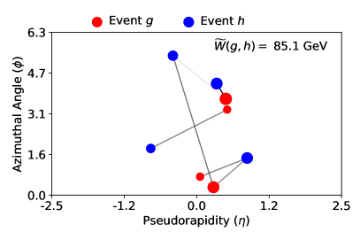
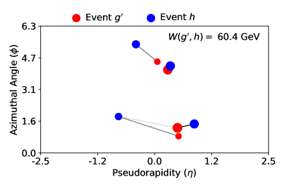
Figure 4: Left: $(\eta,\phi)$-plot of two events $g,h\in\mathcal{G}$. Each point represents a constituent jet, with size proportional to its $p_{T}$ value. A line connecting the $i$-th jet of event $g$ to the $j$-th jet of event $h$ indicates a nonzero value of the optimal coupling $f_{ij}$, with line darkness increasing as a function of the magnitude of $f_{ij}$. Right: $(\eta,\phi)$-plot of events $g^{\prime},h\in\mathcal{G}$, where $g^{\prime}\simeq g$ is an approximate minimizer in equation (5.13). It can be seen that $W(g,h)=W(g^{\prime},h)<\widetilde{W}(g,h)$.

The metric $\widetilde{W}$ does not, however, take into account the equivalence relation $\simeq$ over $\mathcal{G}$ defined in equation (2.2). For example, $\widetilde{W}(g,h)$ could be nonzero even when $g$ and $h$ are deemed equivalent for our purposes. We therefore define our final metric $W$ by

$$W(g,h)=\inf\Big{\{}\widetilde{W}(g^{\prime},h):g^{\prime}\simeq g,\ g^{\prime}\in\mathcal{G}\Big{\}},\quad g,h\in\mathcal{G}.$$ (5.13)

Strictly speaking, $W$ now becomes a metric over the set of equivalence classes of events induced by $\simeq$. We refer to Figure 4 for an illustration. In practice, we numerically approximate $W$ using a procedure described in Appendix C.

6 Simulation Study

6.1 Simulation Description

In this section, we compare the performance of the three background modeling methods OT-FvT, OT-$k$NN and FvT, on realistic simulated collider data, generated using the MadGraph particle physics software (Alwall et al., 2011). Code for reproducing this simulation study is publicly available.

Since $b$-tagging is imperfect, in practice, we expect the $3b$ and $4b$ samples to be composed of a mixture of different multijet scattering processes which do necessarily arise from $b$-quarks. We perform a study in MadGraph to estimate the relative scale of such processes. Assuming a $b$-jet tagging efficiency of 75%, a charm jet tagging efficiency of 15% and a light jet tagging efficiency of 1%, we find that the $4b$ (resp. $3b$) sample consists of 90% (10%) events in a final state with four $b$ quarks, 7% (9%) events in a final state with two $b$ quarks and two charm quarks, and 4% (80%) in a final state with two $b$ quarks and two light quarks. In particular, we stress that a fraction of the $3b$ sample consists of mislabelled $4b$ events, which could be signal events. This signal contamination is expected to be sufficiently small to be considered negligible for purposes of a signal discovery analysis, as in this paper.

We generate four-quark events in MadGraph according to the percentages listed above. The calorimeters in the CMS detector are not perfect, and the measured jet energies have a finite resolution. The distribution of the observed smeared energy is well-approximated by the Gaussian distribution $N(E,\sigma^{2}(E))$, where $E$ denotes the true energy of a jet, and $\sigma(E)$ satisfies

$$\left(\frac{\sigma(E)}{E}\right)^{2}=\left(\frac{S}{\sqrt{E}}\right)^{2}+\left(\frac{N}{E}\right)^{2}+C^{2},$$

for some fixed constants $S,N,C\geq 0$. We apply this smearing to the quark four-vectors, setting $S=0.98,N=0,C=0.054$. For simplicity we set the quark masses to zero and omit them from the the metric $W$. When applying these methods to real data, it may, however, be useful to incorporate the jet masses into the definition of $W$. We also apply jet-level scale factors to account for the $p_{T}$ dependence of CMS $b$-tagging for light, charm and bottom quark jets:

$$\text{Scale Factor}=\begin{cases}(2.5\,p_{T}\,e^{-7\,p_{T}}+0.6)/0.75&\text{$b$-quark}\\ (p_{T}\,e^{-10\,p_{T}}+0.2)/0.15&\text{$c$-quark}\\ (0.03\,p_{T}+0.01)/0.01&\text{$u,d,s$-quark or gluon},\end{cases}$$

where $p_{T}$ is measured in TeV. Events are weighted by the product of the scale factors for the $b$-tagged jets.

Following this pre-processing of the data, the pairing algorithm described in Section 3.2 is applied to all events, and those falling within the Control and Signal Regions are kept. We define these regions according to equations (3.7–3.8), with the parameters $\sigma_{c}=1.03$, $\kappa_{s}=1.6$ and $\kappa_{c}=30$. The final sample consists of $n_{s}=201,568$ events in the $3b$ Signal Region, $n_{c}=159,427$ events in the $3b$ Control Region, $m_{s}=28,980$ events in the 4b Signal Region, and $m_{c}=22,053$ events in the 4b Control Region. The order of magnitude of these sample sizes, as well as the proportion of $3b$ to $4b$ events, is similar to those used in recent di-Higgs analyses at the LHC (ATLAS, 2019a). We further simulate a separate 4b sample of size approximately $10(n_{s}+m_{s})$, which we choose not to contain any signal events, and whose distribution we treat as the ground truth for the purpose of validating our background models.

We additionally generate a Monte Carlo sample from the SM di-Higgs signal distribution, with which the signal intensity rates $(S_{j})_{j=1}^{J}$, used to form the likelihood function (3.5), can be specified. For the purpose of validating our background models, we train a $[0,1]$-valued classifier $\widehat{\xi}$ (abbr. Signal vs. Background, or SvB, classifier) to discriminate the $4b$ data from the Monte Carlo di-Higgs sample. Given that our simulated 4b sample contains no signal events, $\widehat{\xi}$ forms a reasonable proxy for the theoretical binning function $\xi$ in equation (3.6). The SvB classifier has the same architecture as that of the FvT classifier described in Appendix B. In the sequel, we refer to $\widehat{\xi}(g)$ as the SvB value corresponding to an event $g$.

Finally, we discuss our choice of the parameter $R$ arising in the definition of the metric $W$. In order for the two terms in the definition of $\widetilde{W}$ to be of comparable order, we make the requirement that $R$ lie within the range of the first summand in equation (5.12). We identify this range as follows. Since $b$-tagging is only performed for values of $\eta$ lying in the interval $[-2.5,2.5]$, we impose $R\leq\sqrt{\pi^{2}+5^{2}}\approx 5.9$. Furthermore, jet clustering algorithms used by CMS merge particles whose $(\eta,\phi)$-Euclidean distance is within $0.4$ (Cacciari, Salam and Soyez, 2008; CMS, 2017), thus we impose $R\geq 0.4$. Now, since we expect that the largest discrepancies between the Control and Signal Region distributions arise in the kinematic variables $(\eta,\phi)$, we choose the smallest possible value $R=0.4$ when fitting the empirical optimal transport coupling $\widehat{\pi}$. On the other hand, for the nearest-neighbor lookup of the OT-$k$NN method, we set $R=2.75$, which is the midpoint of the interval $[0.4,5.9]$. We make no attempt to tune these values of $R$, and we leave open the question of choosing them in a data-driven fashion. We compute the metric $W$ in part using the EnergyFlow Python library (Komiske, Metodiev and Thaler, 2022), and we compute optimal couplings between distributions of collider events using the Python Optimal Transport library (Flamary et al., 2021)—see Appendix D for further details.

6.2 Simulation Results

The fitted intensity measures $\widehat{\beta}_{4}^{s}$ produced by the three background methods (FvT, OT-$k$NN and OT-FvT) are binned and plotted in Figure 5. Logarithmic scales are used to better visualize signal-rich regions. Plots with additional kinematic variables are given in Appendix E.

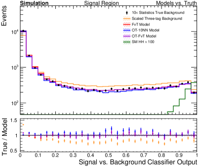
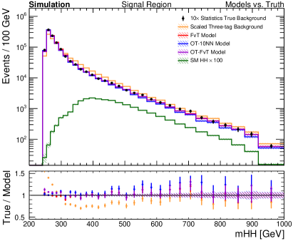
Figure 5: Histograms of the the SvB classifier output variable (left) and the $m_{\mathrm{HH}}$ variable (right) for the three background models as well as the upsampled 4b data (treated as the ground truth), the 3b data (normalized by the factor $n_{s}m_{c}/n_{c}$), and the di-Higgs signal sample (SM HH). Error bars in the $k$-th bin of any histogram denote $\pm\sqrt{N_{k}}$, where $N_{k}$ is the number of events per bin. Error bars in the ratio plot denote $\pm\sqrt{N_{k}}/N_{0k}$, where $N_{0k}$ is the number of observed $4b$ events per bin. The dashed lines in the ratio plot denote $\pm\sqrt{1/N_{0k}}$.

It can be seen that the three methods yield qualitatively similar estimates of the SvB intensity function. We recall that the SvB variable is of primary interest to model, as it is used as the final discriminant when testing the signal hypothesis (3.1). The $m_{\mathrm{HH}}$ variable has also been used as the final discriminant in recent di-Higgs studies (Bryant, 2018). Given an event $g\in\mathcal{G}$ with dijet pairing $\{g^{1},g^{2}\}$, its $m_{\mathrm{HH}}$ value is defined as follows, using the notation of Section 3.2,

$$m_{\text{HH}}(g)=m\bigg{(}\frac{m_{\text{H}}}{m(g^{1})}g^{1}+\frac{m_{\text{H}}}{m(g^{2})}g^{2}\bigg{)}.$$ (6.1)

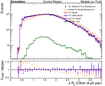
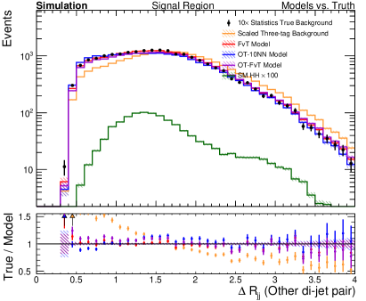
Figure 13: Histograms of the “$\Delta R_{jj}$–Other” variable (defined as the angular distance between the two jets of an event other than the two which are closest) in the Control Region (left) and the Signal Region (right), for the three background models as well as the upsampled 4b data (treated as the ground truth), the 3b data (normalized by the factor $n_{s}m_{c}/n_{c}$), and the di-Higgs signal sample (SM HH). .

Once again, we observe that this variable is well-modelled by all three methods. Among the various kinematic variables which we analyzed, the “$\Delta R_{jj}$–Other” variable, appearing in Figure 13 of Appendix E, presents one of the largest qualitative discrepancies between the three methods, and appears to be best-modelled by the FvT method. In all cases, it can be seen that the three methods provide a significant improvement compared to the uncorrected $3b$ sample.

In order to provide a quantitative comparison of these methods, we develop a heuristic two-sample test for testing equality between the distribution of the fitted background models and of the true upsampled $4b$ data. Specifically, we form a proxy for a two-sample test by training classifiers to discriminate each of the background estimates from the upsampled $4b$ data. Intuitively, if a background estimate is accurate, then a classifier should not be able to tell it apart from the true data. For each classifier, we record the area under the receiver operating characteristic curve (AUC; Hanley and McNeil (1982)), and any deviation of this quantity from .5 is an indication of mismodeling. We again choose our classifiers to be residual neural networks with the architecture described in Appendix B. Although this choice is inherently favourable to the FvT method, and to some extent the OT-FvT method, we use it because it also coincides with the SvB classifier architecture, and will thus be most powerful at detecting mismodeling in the features which are relevant for the final signal analysis.

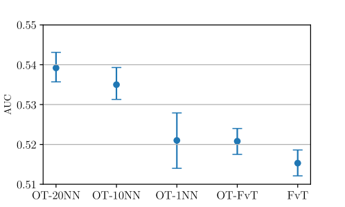
Figure 6: A Fitted AUC values obtained by discriminating each background model from the upsampled 4b data using the FvT classifier, together with 95% percentile bootstrap variability intervals, obtained by bootstrapping the predicted classifier probabilities. 1,000 bootstrap replications are used. Note that this bootstrap procedure does not take into account the variability of the background estimators themselves. For the $3b$-tagged data, we obtain the AUC 0.5843, with variability interval [0.5812,0.5874].

The fitted AUC value for each method is reported in Figure 6. Though all AUCs are significantly greater than .5, they are substantially lower for our background models than for the benchmark method consisting of the uncorrected 3b sample. The FvT method has the lowest AUC, followed closely by the OT-FvT method and OT-$k$NN method. While the OT-1NN method has comparable AUC point estimate as the OT-FvT method, we emphasize that its variability interval is wider, which could have been anticipated from the discussion in Section 5.2.5, where we emphasized that the support size of $\beta_{4,1\mathrm{NN}}^{s}$ can be an order of magnitude smaller than $n_{s}$. In contrast, the OT-10NN and OT-20NN estimators have narrower variability intervals than OT-1NN, but have markedly larger AUC point estimates than the remaining methods. The performance of the OT-$k$NN method for varying values of $k$ is also illustrated in Figure 8 along as a function of the SvB and $m_{\mathrm{HH}}$ variables.

We next provide a qualitative comparison of the fitted weights produced by the three background modeling methods. Recall that these methods all take the form

$$\widehat{\beta}_{4}^{s}=\sum_{i=1}^{n_{s}}v_{i}\delta_{H_{i}^{s}},$$

for some nonnegative weights $v_{i}$, which are summarized up to normalization in Table 1. In Figure 8, we plot the weights of the two optimal transport methods against those of the FvT method. We observe that the FvT and OT-FvT methods produce weights which are concentrated and symmetric around the identity. This implies that the odds ratio of the FvT classifier at a point $H_{j}^{s}$ in the Signal Region behaves similarly to the odds ratio at any point $H_{i}^{c}$ in the Control Region to which $H_{j}^{s}$ is optimally coupled. This suggests that the transfer learning of the FvT classifier from the Control Region to the Signal Region is, to some extent, well-modelled by the optimal transport coupling $\widehat{\pi}$. This observation heuristically suggests that Assumptions 1–2 both hold in this simulation. In contrast to the method OT-FvT, we observe that the method OT-10NN produces markedly different weights than the FvT method, which can partly be anticipated from the discrete nature of the nearest neighbor extrapolation. We conjecture that the nearest-neighbor estimator of the optimal transport coupling has poorer theoretical risk than its counterpart in the OT-FvT method.

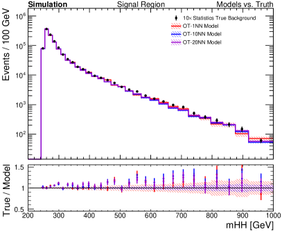
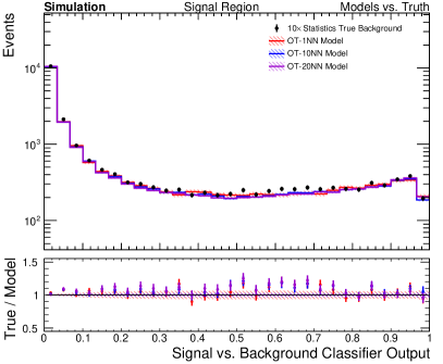
Figure 7: Histograms of the SvB classifier output variable (left) and the $m_{\mathrm{HH}}$ variable (right) for the OT-$k$NN estimator, with $k\in\{1,10,20\}$.

7 Conclusion and Discussion

Our aim has been to study the problem of data-driven background estimation, motivated by the ongoing search for double Higgs boson production in the $4b$ final state. After recalling a widely-used approach to this problem based on transfer learning of a multivariate classifier, our first contribution was to develop the FvT classifier architecture which is tailored to collider data, and which can serve as a powerful tool for implementing this methodology. Our primary contribution was then to propose a distinct background estimation method based on the optimal transport problem. A recurring theme throughout our work has been the complementarity of the modeling assumptions made by these two distinct approaches, which allows them to be used as cross-checks for one another in practice. We substantiate this point with a realistic simulation study, in which these methodologies appear to give consistent results despite their inherently distinct derivations.

Quantifying the uncertainty of our background estimates is a challenging problem left open by our work, which is nonetheless crucial for applying our methods in practice. In the experimental particle physics community, it is commonplace to measure both statistical uncertainties—those arising from fluctuations of the data generating process—and systematic uncertainties—those arising from potential mismodeling (Heinrich and Lyons, 2007). Both of these forms of uncertainty are challenging to quantify in our context. For instance, a prerequisite for quantifying the statistical uncertainty of the methods OT-$k$NN or OT-FvT is to perform statistical inference for optimal transport maps. This is a difficult open problem in the statistical optimal transport literature, that has only been addressed for some special cases (Rippl, Munk and Sturm, 2016; Ramdas, Trillos and Cuturi, 2017), and for regularized variants of optimal transport maps which differ from those used in our work (Klatt, Tameling and Munk, 2020; Gunsilius and Xu, 2021; González-Sanz, Loubes and Niles-Weed, 2022; Goldfeld et al., 2022). The question of quantifying systematic uncertainties is more open-ended, and typically involves heuristics for assessing the extent of potential mismodeling by the background estimation methods. Due to the complementarity of assumptions placed by our methods, any lack of closure between them could potentially play a role in quantifying their systematic uncertainties. While further investigation is required to make such a proposal formal, it is our hope that the optimal transport methodology presented in our work can help contribute to the challenging question of systematic uncertainty quantification in the search for di-Higgs boson production, or in other searches at the Large Hadron Collider.

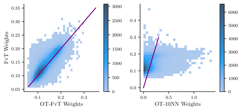
Figure 8: Bivariate histogram of the $3b$ data $H_{1}^{s},\dots,H^{s}_{n_{s}}$ in the Signal Region, plotted in terms of the weights of the OT-FvT method against those of the FvT method (left), and of the OT-10NN method against those of the FvT method (right). The purple lines denote the identity function.

[Acknowledgments]

We are grateful to the CMU Statistical Methods for the Physical Sciences (STAMPS) research group for insightful discussions and feedback throughout this work.

This work was supported in part by NSF PHY-2020295 and NSF DMS-2053804. TM was supported in part by the Natural Sciences and Engineering Research Council of Canada (NSERC), through a PGS D Scholarship.

Appendix A Translation for the high-energy physicist

The main body of the text has been primarily written with the statistics community in mind. This appendix aims to bridge the gap between the language and formalism used by statisticians and that common in high-energy physics (HEP).

Section 3.1 describes the standard HEP search formalism in the statistician’s nomenclature. We have a dataset $F$ consisting of background and some a priori unknown amount of signal, parameterized by signal strength $\mu$. The search is done in bins of a discriminating variable $\xi$, which will—later in the text—be taken to be the output of a multivariate classifier trained to separate signal and background. The challenge is to predict the amount of background in each of the classifier output bins.

The discussion relating to Borel measures is a formality that can be safely ignored by less technical readers. These technicalities are relevant because our discussion of the optimal transport problem, below, is more naturally formulated in terms of distributions over sets of events rather than probability density functions. Distributions are restricted to the Borel $\sigma$-algebra to avoid theoretically possible pathologies, which are unlikely to be of practical concern to the data analyst.

“Intensity measures” have a normalization given by the expected number of events, whereas “probability distributions” are normalized to unity. For example, $\beta_{4}$ is the intensity of background events, with $\beta_{4}(\mathcal{G})$ the expected total number of these events. Later on, we will also use the notation $b_{4}$ to denote an “intensity function”, which can be viewed as the unnormalized probability density function corresponding to the intensity measure $\beta_{4}$.

Section 3.2 introduces the three-tag dataset $T$. The three-tag data, when normalized to the number of four-tag events, provides a zeroth order estimate of the $4b$ background. The main contribution of our work is in deriving corrections to the $3b$ data to better approximate the true $4b$ background.

An algorithm is used to pair jets into Higgs candidates and Signal and Control regions are defined using the reconstructed masses. The “empirical estimators of the measures $\beta_{3}^{c},\beta_{3}^{s},\beta_{4}^{c}$” are effectively just the observed datasets in the respective regions.

Section 4 describes a data-driven background estimation method used frequently in HEP (ATLAS, 2018a; CMS, 2022). This method can be thought of as an extension of the “ABCD method”.

Equation (4.1) points out that a probabilistic classifier ($\psi$) trained to separate $4b$ and $3b$ events can be used to define a function that returns the relative probability density ratios between $4b$ and $3b$ events. This density ratio can then be used to weight the $3b$ data to give an improved estimate of the $4b$ background.

We train a classifier, referred to as the “FvT classifier”, to separate $4b$ and $3b$ data in the Control Region (CR). Assumption 1 formalizes the usual assumption that the classifier trained with events in the CR can be safely extrapolated to also weight $3b$ events in the Signal Region (SR). With this assumption the predicted background in the SR can be obtained by weighting $3b$ SR events by the density ratio estimated in the CR, equation (4.4).

Section 5 presents a novel method for implementing the ABCD method across phase space. Instead of extrapolating between the $3b$ and $4b$ samples—assuming the extrapolation is the same in the CR and SR—we propose extrapolating between the CR and SR—assuming the extrapolation is the same in the $3b$ and $4b$ samples. The extrapolation across phase space is complicated because the CR and SR distributions are kinematically disjoint. We cannot use a classifier to correct kinematic differences between the samples; any classifier trained on kinematically disjoint samples would achieve perfect separation, and the corresponding weights would be undefined. Instead, we assume that the “optimal transport” map which maps events in the CR to the SR is the same for the $3b$ and $4b$ events. The optimal transport (OT) map is the transformation that minimizes the “cost” in deforming a distribution supported in the CR into one supported in the SR. The idea is to find the optimal map between the $3b$ CR and $3b$ SR events and then “apply the map” to the $4b$ CR events.

Neither finding, nor applying the OT map is straightforward; Sections 5.1 and 5.2.1 explain how the OT map is estimated and Sections 5.2.2 and 5.2.3 presents two alternative methods for applying the map to $4b$ CR events. In order to define the OT problem, we need a notion of cost, or distance, between events; our choice is presented in Section 5.3.

Section 5.1 describes complications associated with estimating the OT maps with collider data. Formally, the OT problem is known to have a unique solution on continuous distributions with a Euclidean cost function; however, we have a non-Euclidean cost function (see Section 5.3) and only have access to finite datasets drawn from the relevant probability distributions. So instead of solving for the OT map, we estimate a “coupling” between datasets that converges to the OT map in the infinite statistics limit. This coupling is the solution of the “Kantorovich optimal transport problem” defined in equation (5.3) and is a (weighted) mapping of events in the $3b$ CR to events in the $3b$ SR. Assumption 2 formalizes the assumption that the map fit with the $3b$ data is applicable to the $4b$ events.

Section 5.2.1 explains that the coupling is estimated using the observed $3b$ CR and SR events. Note that this coupling map is only defined for $3b$ CR events, whereas we need to apply it to $4b$ CR events to get a background estimate. We have two different solutions for applying the OT map “out-of-sample” to $4b$ events, which are described in Sections 5.2.2 and 5.2.3. Both of these methods rely on the fact that $3b$ and $4b$ CRs share the same support.

Section 5.2.2 presents the first solution (called OT-$k$NN), in which $4b$ CR events are mapped to the “nearest” $3b$ CR events. The OT coupling of these nearest neighbors is then used to map the $4b$ CR event to the SR. We can use an arbitrary number of nearest neighbors ($k$), where the neighbors are weighted based on how close they are to the input $4b$ CR event. Again, in order for this to make sense we need a notion of distance between events, and we use the definition presented in Section 5.3.

Section 5.2.3 presents the second solution (called OT-FvT) for applying the OT map to $4b$ events. Here, the $3b$ CR events are first weighted to look like the $4b$ CR events using the FvT classifier. Note that, in this case, the FvT-weights are applied in-sample and thus no assumption of extrapolation is required. The weighted $3b$ events both emulate the $4b$ CR distribution and have OT couplings defined; they can thus be mapped to the SR directly.

Section 5.2.4 describes how the overall background normalization is determined. For technical reasons, the coupling maps fit the normalized distributions, i.e., they only predict the background shapes. The overall normalization is determined using the standard ABCD method.

Appendix B The FvT Classifier for Collider Events

The aim of this appendix is to describe the architecture of the FvT classifier defined in Section 4. Recall that our aim to design a classifier $\widehat{\psi}$ over $\mathcal{G}$, which

1. is invariant to the ordering of the constituent jets in an input event $g$;

2. is invariant with respect to the equivalence relation $\simeq$ defined in (2.2);

3. incorporates the dijet substructure of an event $g=g^{1}+g^{2}$.

We opt for a convolutional neural network architecture with residual layers, or ResNet (He et al., 2016), as depicted in Figure 9. One dimensional convolutions are used to project pairs of jets into dijets and pairs of dijets into quadjets. These convolutions are just linear maps

$$\sum_{i,\alpha}v_{i}^{\alpha}w_{i}^{\alpha,\beta}+b^{\beta}=v^{\beta}$$ (B.1)

where $i$ is summed over the pair of input objects and $\alpha$ is summed over the input object features to produce an output in feature space indexed by $\beta$. The learnable parameters are the $w_{i}^{\alpha,\beta}$ weight matrix and the $b^{\beta}$ bias vector. There is only one such set of learnable parameters for a given convolutional layer and it is applied to each pair of input objects to produce the output objects. There are thus $I\times A\times B+B$ learnable parameters for each convolution layer where $I$ is the number of input objects, $A$ is the dimension of the input object feature space and $B$ is the dimension of the output object feature space. An input event $g=\sum_{j=1}^{4}p_{T_{j}}\delta_{(\eta_{j},\phi_{j},m_{j})}$ to the network is treated as a one-dimensional image with 4 pixels, where each pixel corresponds to one jet parametrized by its coordinates $(p_{T_{j}},\eta_{j},\phi_{j},m_{j})$. The layers of the network are then designed as follows:

1. The 4 input pixels are duplicated twice to obtain an image with 12 pixels, such that all 6 possible pairs of dijets appear exactly once, consecutively in the image. Each such pair is then convolved into a one-dimensional image of six dijet pixels.

2. Each pair of dijets from this image is further convolved into an image with three pixels, consisting of the three possible pairing representations of the original four-jet, or quadjet, event.

3. The three quadjet pixels are combined into the last pixel representing the whole event.

4. A final output layer passes the event through a softmax activation function to produce the fitted probability $\widehat{\psi}(g)$.

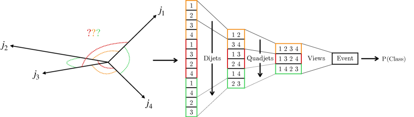
Figure 9: Illustration of the FvT classifier architecture. The classifier takes as input an event with four jets, passes it through the layers (1–4) of the network described below, and outputs the fitted probability that the event arose from the $4b$ distribution as opposed to the $3b$ distribution.

Notice that (c) is satisfied by the construction of the network. We partially impose (a) by replacing pairs of dijet pixels $\{d_{i},d_{j}\}$ in step (ii) by their sums and absolute values of their differences as follows:

$$\{d_{i},\,d_{j}\}\rightarrow\{(d_{i}+d_{j})/2,\,|d_{i}-d_{j}|/2\}$$ (B.2)

In this way, the dijet to quadjet feature learning is invariant under the permutation

$$\{d_{i},\,d_{j}\}\rightarrow\{d_{j},\,d_{i}\}.$$

Similar modifications may be made in (i) to render the network entirely invariant to relabeling of the input jets, as in (a), but we have observed increased performance by allowing the convolutions in step (i) to have information about the $p_{T}$ ordering of the jets. Quadjet pixels $q_{i}^{\alpha}$ from (ii) are added together to produce a single event level pixel $e^{\alpha}$ weighted by a real-valued score $s_{i}$ in step (iii) to guarantee permutation invariance of the three pixels:

$$e^{\alpha}=\sum_{i}s_{i}e_{i}^{\alpha}.$$

The quadjet scores are the softmax over quadjets of the dot product between quadjet features and a learned reference vector $w^{\alpha}$:

$$s_{i}=\text{Softmax}\left[\sum_{\alpha}q_{i}^{\alpha}w^{\alpha}\right].$$

To enforce (b), recall that the network should be invariant under transformations $F_{1}^{-}:\eta\mapsto-\eta$, $F_{2}^{-}:\phi\mapsto-\phi$ and $F_{2}^{\Delta}:\phi\mapsto\phi+\Delta$, for any $\Delta\in[0,2\pi)$, when applied simultaneously across all constituent jets of an event. Invariance under $\eta$ flips is enforced by computing the first several layers twice, with and without the flip, and then averaging the resulting quadjet pixels prior to step (iii). In principle, the same may be done to enforce invariance under the rotation $F^{\Delta}$ by averaging over a large grid of candidate values $\Delta$. To reduce the computational burden which would arise from such an operation, we instead apply random rotations $\Delta$ at each batch used in the Adam optimizer (Kingma and Ba, 2015) which we choose for training the network.

In steps (i)-(iii), we also add engineered features specifically designed for dijet, quadjet, and event-level pixels, respectively. These engineered features are designed such that they preserve invariance properties (a) and (b). For instance, in step (i) we insert pixels containing dijet masses and the Euclidean distance between dijet angular variables $\eta_{i},\phi_{i}$.

Appendix C Metric Approximation

This section describes how we numerically approximate equation (5.13) taking into account the equivalence relation $\sim$ on $\mathcal{G}$. As discussed in Section 2.2, events are deemed equivalent up to relative rotations in $\phi$ and relative reflections about the $x$- and $z$- axes. The distance between a source and a target event is taken to be the minimum value of the metric $W$ between the target event and all events in the equivalence class of the source event. The left plot of Figure 10 shows an example of this calculation. The metric $W$ between two events is shown as a function of the overall $\phi$ offset ($\Delta\phi$) of the source event. The solid blue line shows the result with the nominal orientation of the axes in the source event; the dashed blue line is the result after reflecting the source event about the $z$-axis; the red curves show the results after reflection about the $x$-axis (solid red) and after a reflection of both the $x$- and $z$-axes (dashed red). The black dot shows the global minimum; this is the value of the final metric $\widetilde{W}$ defined in equation (5.13).

A brute force calculation of the minimizer in the definiton of $\widetilde{W}$ is slow. The results shown in the left plot of Figure 10 require 400 individual calculations of the metric $W$: 100 for each scan in $\Delta\phi$. Each of these individual calculations is costly as they involve solving an optimal transport problem between collider events.

We speed up the calculation of the metric by approximating the value of $\widetilde{W}$ using an estimate of the relative $z$-axis orientation and of the $\phi$-offset of the source event that achieves the minimum in equation (5.13). The orientation of the $z$-axis of the global minimum can be estimated by calculating the sum of the $z$-components of the jet momenta for each event $g=\sum_{i=1}^{K}p_{T_{i}}\delta_{(\eta_{i},\phi_{i},m_{i})}$:

$$S_{z}\equiv\sum_{i=1}^{K}p_{T_{i}}\cos(\theta_{i})=\sum_{i=1}^{K}p_{T_{i}}\sinh(\eta_{i}).$$ (C.1)

The global EMD minimum tends to occur when the relative orientations of the source and target event $z$-axes produce the same sign of $S_{z}$. We thus reflect the $z$-axis of the source event if the $S_{z}$ sums of the source and target events have opposite signs.

We estimate the relative $\phi$-offset of the global minimum using the transverse thrust axis. The transverse thrust axis is defined as the unit vector in the $(x,y)$-plane with angle $\phi_{\rm{thrust}}$ such that the sum of the jet $p_{T}$ projections along the unit vector are maximized:

$$\phi_{\rm{thrust}}=\operatorname*{argmax}_{\phi\in[0,2\pi)}\sum_{i=1}^{K}p_{T_{i}}\cos(\phi_{i}-\phi).$$ (C.2)

The relative $\phi$ rotation that achieves the minimum in the definition of $\widetilde{W}$ will tend to either align or anti-align the thrust axes of the events. We estimate the value of $\widetilde{W}$ by taking the minimum of the $W$ calculated four times: with the source and target thrust axes either aligned or anti-aligned, and with the source $x$-axis either nominal or reflected. The green line in the left plot of Figure 10 shows the estimated value of the minimum in $\widetilde{W}$ using this algorithm. Our estimation of $\widetilde{W}$—requiring only 4 individual evaluations of $W$—agrees well with the brute force calculation—using 400 individual EMD evaluations.

The right plot of Figure 10 shows the performance of our approximation on a sample of events. The blue distribution compares the relative bias in our estimate with respect to the minimum calculated by brute force. The majority of events have a bias of at most a few percent. For reference, the red distribution shows the relative bias of the EMD calculated using the nominal event.

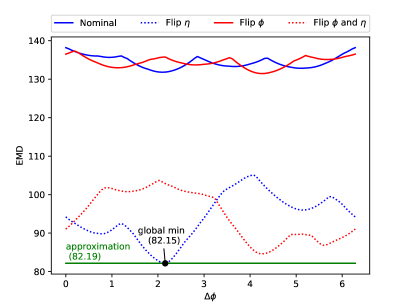
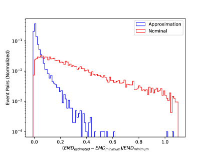
Figure 10: Example of the calculation of $\widetilde{W}$ for a single pair of events (left), and performance of our approximation on a sample of events (right). The relative bias of our approximation is shown in blue. The bias using the nominal input events is shown in red.

Appendix D Computation of Optimal Transport Couplings

In this section, we describe our numerical approximation of the empirical optimal transport coupling $\widehat{q}$ in equation (5.6). Equation (5.6) is a linear program which can be computed exactly using simplex algorithms (Peyré and Cuturi, 2019). Such approaches have memory complexity which grows quadratically in $n_{c}\wedge n_{s}$, since they require the cost matrix

$$C=(W(H_{i}^{c},H_{j}^{s}):1\leq i\leq n_{c},1\leq j\leq n_{s})$$

to be stored in memory. As described in Section 6, the sample sizes $n_{c}$ and $n_{s}$ are at least of the order $10^{5}$ in our problem, in which case the storage of the matrix $C$ becomes intractable. For low-dimensional problems, the storage of $C$ can be avoided by using the so-called back-and-forth algorithm of Jacobs and Léger (2020), which has linear memory complexity. For higher dimensional problems, a common approach is to divide the datasets into several (say, $B$) batches, and to compute $B$ separate optimal transport couplings. Such batches can either be obtained through subsampling or deterministic schemes—see Sommerfeld et al. (2019), Fatras et al. (2021), Nguyen et al. (2022), and references therein.

We follow a similar approach in our work. We partition the two samples

$$\mathcal{D}^{c}=\{H_{1}^{c},\dots,H_{n_{c}}^{c}\},\quad\mathcal{D}^{s}=\{H_{1}^{s},\dots,H_{n_{s}}^{s}\}$$

into $B\geq 1$ disjoint batches $\mathcal{D}_{1}^{c},\dots,\mathcal{D}_{B}^{c}$ and $\mathcal{D}_{1}^{s},\dots,\mathcal{D}_{B}^{s}$, satisfying $\mathcal{D}^{c}=\bigcup_{k}\mathcal{D}_{k}^{c}$ and $\mathcal{D}^{s}=\bigcup_{k}\mathcal{D}_{k}^{s}$. Assume for simplicity that for some $n_{B}^{c},n_{B}^{s}\geq 1$, $|\mathcal{D}_{k}^{c}|=n_{c}^{B}$ and $|\mathcal{D}_{k}^{s}|=n_{s}^{B}$ for all $k=1,\dots,B$. We then compute the optimal transport couplings

$$\widehat{q}^{k}=\operatorname*{argmin}_{(q_{ij})\subseteq\mathbb{R}^{n_{c}^{B}\times n_{s}^{B}}}\sum_{H^{c}\in\mathcal{D}_{k}^{c}}\sum_{H^{s}\in\mathcal{D}_{k}^{s}}q_{ij}W(H^{c},H^{s})$$

where the minimum is taken over all $q_{ij}\geq 0$ satisfying

$$\sum_{i=1}^{n_{c}^{B}}q_{ij}=\frac{1}{n_{s}^{B}},\quad\sum_{j=1}^{n_{s}^{B}}q_{ij}=\frac{1}{n_{c}^{B}},$$

for all $k=1,\dots,B$. We then approximate the empirical optimal transport coupling $\widehat{q}$ in equation (5.6) by the matrix

$$\widetilde{q}=\frac{1}{B}\begin{pmatrix}\widehat{q}^{1}&&&\\ &\widehat{q}^{2}&&\\ &&\ddots&\\ &&&\widehat{q}^{B}\end{pmatrix}.$$

The memory complexity of this algorithm is $O(Bn_{c}^{B}n_{s}^{B})$ as opposed to the complexity $O(n_{c}n_{s})$ incurred by any method which requires the storage of the matrix $C$.

In our simulations, we computed the couplings $\widehat{q}_{k}$ using the network simplex solver described by Bonneel et al. (2011), as implemented in the Python Optimal Transport package (Flamary et al., 2021). Our simulations were run on a standard Linux machine with 12 cores and 32GB of RAM. We chose $B=16$, which is approximately the smallest value of $B$ for which the computation of the couplings $\widehat{q}^{k}$ did not exceed our machine’s memory limit.

We chose the batches according to the following procedure. For any event $G=\sum_{j=1}^{4}p_{T_{j}}\delta_{(\eta_{j},\phi_{j},m_{j})}$, let $s_{T}(G)=\sum_{j=1}^{4}p_{T_{j}}$ denote the scalar sum of the transverse momenta of $G$. Let $H_{(i)}^{c}$ denote the event among $H_{1}^{c},\dots,H_{n_{c}}^{c}$ with the $i$-th smallest $s_{T}$ value, for all $i=1,\dots,n_{c}$. That is,

$$s_{T}(H_{(1)}^{c})\leq s_{T}(H_{(2)}^{c})\leq\dots\leq s_{T}(H_{(n_{c})}^{c}).$$

We likewise define $H_{(j)}^{s}$ for $j=1,\dots,n_{s}$ such that

$$s_{T}(H_{(1)}^{s})\leq s_{T}(H_{(2)}^{s})\leq\dots\leq s_{T}(H_{(n_{s})}^{s}).$$

We then set, for $k=1,\dots,B$,

$$\mathcal{D}_{k}^{c}=\{H_{(B(r-1)+k)}^{c}:1\leq r\leq n_{c}^{B}\},\quad\mathcal{D}_{k}^{s}=\{H_{(B(r-1)+k)}^{s}:1\leq r\leq n_{s}^{B}\}.$$

This choice ensures that each batch contains events with a comparable range of $s_{T}$ values. We impose this property because the penalty term in the definition of $\widetilde{W}$ (Eq. (5.12)) is sensitive to large deviations of $s_{T}$ values. We leave open for future work whether different batching methods, such as subsampling, would yield improved performance.

Appendix E Additional Simulations Results

In this appendix, we report additional results from the simulation study in Section 6.

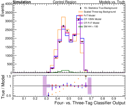
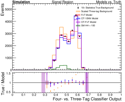
Figure 11: Histograms of the FvT classifier output variable in the Control Region (left) and the Signal Region (right), for the three background models as well as the upsampled 4b data (treated as the ground truth), the 3b data (normalized by the factor $n_{s}m_{c}/n_{c}$), and the di-Higgs signal sample (SM HH). .

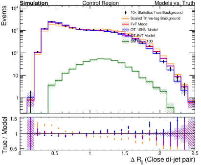
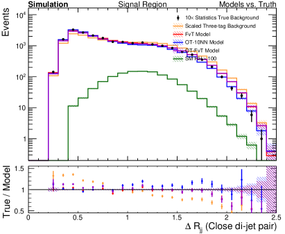
Figure 12: Histograms of the “$\Delta R_{jj}$–Close” variable (defined as the angular distance between the two closest jets of an event) in the Control Region (left) and the Signal Region (right), for the three background models as well as the upsampled 4b data (treated as the ground truth), the 3b data (normalized by the factor $n_{s}m_{c}/n_{c}$), and the di-Higgs signal sample (SM HH). .

References

- Alison (2015) {bphdthesis}[author] \bauthor\bsnmAlison, \bfnmJohn\binitsJ. (\byear2015). \btitleThe Road to Discovery: Detector Alignment, Electron Identification, Particle Misidentification, WW Physics, and the Discovery of the Higgs Boson, \btypePhD thesis \bnotePresented 08 Nov 2012. \bdoi10.1007/978-3-319-10344-0 \endbibitem
- Alwall et al. (2011) {barticle}[author] \bauthor\bsnmAlwall, \bfnmJohan\binitsJ., \bauthor\bsnmHerquet, \bfnmMichel\binitsM., \bauthor\bsnmMaltoni, \bfnmFabio\binitsF., \bauthor\bsnmMattelaer, \bfnmOlivier\binitsO. and \bauthor\bsnmStelzer, \bfnmTim\binitsT. (\byear2011). \btitleMadGraph 5: going beyond. \bjournalJournal of High Energy Physics \bvolume2011 \bpages128. \endbibitem
- ATLAS (2012) {barticle}[author] \bauthor\bsnmATLAS (\byear2012). \btitleObservation of a new particle in the search for the Standard Model Higgs boson with the ATLAS detector at the LHC. \bjournalPhysics Letters B \bvolume716 \bpages1–29. \endbibitem
- ATLAS (2015) {barticle}[author] \bauthor\bsnmATLAS (\byear2015). \btitleObservation and measurement of Higgs boson decays to WW∗ with the ATLAS detector. \bjournalPhys. Rev. D \bvolume92 \bpages012006. \bdoi10.1103/PhysRevD.92.012006 \endbibitem
- ATLAS (2018a) {barticle}[author] \bauthor\bsnmATLAS (\byear2018a). \btitleSearch for pair production of higgsinos in final states with at least three b-tagged jets in 13 TeV pp collisions using the ATLAS detector. \bjournalPhysical Review D \bvolume98. \bdoi10.1103/physrevd.98.092002 \endbibitem
- ATLAS (2018b) {barticle}[author] \bauthor\bsnmATLAS (\byear2018b). \btitleObservation of decays and production with the ATLAS detector. \bjournalPhysics Letters B \bvolume786 \bpages59–86. \endbibitem
- ATLAS (2018c) {barticle}[author] \bauthor\bsnmATLAS (\byear2018c). \btitleMeasurements of Higgs boson properties in the diphoton decay channel with 36 fb- 1 of p p collision data at s= 13 TeV with the ATLAS detector. \bjournalPhysical review D \bvolume98 \bpages052005. \endbibitem
- ATLAS (2018d) {binproceedings}[author] \bauthor\bsnmATLAS (\byear2018d). \btitleMeasurement of gluon fusion and vector-boson-fusion Higgs boson production cross-sections in the decay channel in pp collisions at TeV with the ATLAS detector. \bpublisherATLAS-CONF-2018-004. \endbibitem
- ATLAS (2018e) {binproceedings}[author] \bauthor\bsnmATLAS (\byear2018e). \btitleMeasurements of the Higgs boson production, fiducial and differential cross sections in the decay channel at TeV with the ATLAS detector. \bpublisherATLAS-CONF-2018-018. \endbibitem
- ATLAS (2019a) {barticle}[author] \bauthor\bsnmATLAS (\byear2019a). \btitleSearch for pair production of Higgs bosons in the final state using proton-proton collisions at TeV with the ATLAS detector. \bjournalJournal of High Energy Physics \bvolume2019 \bpages30. \bdoi10.1007/JHEP01(2019)030 \endbibitem
- ATLAS (2019b) {barticle}[author] \bauthor\bsnmATLAS (\byear2019b). \btitleCross-section measurements of the Higgs boson decaying into a pair of -leptons in proton-proton collisions at TeV with the ATLAS detector. \bjournalPhys. Rev. D \bvolume99 \bpages072001. \bdoi10.1103/PhysRevD.99.072001 \endbibitem
- ATLAS (2021) {barticle}[author] \bauthor\bsnmATLAS (\byear2021). \btitleSearch for the HH process via vector-boson fusion production using proton-proton collisions at TeV with the ATLAS detector. \bjournalJournal of High Energy Physics \bvolume2021. \bdoi10.1007/jhep01(2021)145 \endbibitem
- ATLAS (2022) {btechreport}[author] \bauthor\bsnmATLAS (\byear2022). \btitleSearch for non-resonant pair production of Higgs bosons in the final state in collisions at TeV with the ATLAS detector \btypeTechnical Report, \bpublisherCERN, \baddressGeneva \bnoteATLAS-CONF-2022-035. \endbibitem
- ATLAS, CMS and Higgs Combination Group (2011) {barticle}[author] \bauthor\bsnmATLAS, \bauthor\bsnmCMS and \bauthor\bsnmHiggs Combination Group (\byear2011). \btitleProcedure for the LHC Higgs boson search combination in Summer 2011. \bnoteCMS-NOTE-2011-005. ATL-PHYS-PUB-2011-11. \endbibitem
- Barlow (1987) {barticle}[author] \bauthor\bsnmBarlow, \bfnmRoger\binitsR. (\byear1987). \btitleEvent Classification Using Weighting Methods. \bjournalJournal of Computational Physics \bvolume72 \bpages202–219. \endbibitem
- Behnke et al. (2013) {bbook}[author] \bauthor\bsnmBehnke, \bfnmOlaf\binitsO., \bauthor\bsnmKröninger, \bfnmKevin\binitsK., \bauthor\bsnmSchott, \bfnmGrégory\binitsG. and \bauthor\bsnmSchörner-Sadenius, \bfnmThomas\binitsT. (\byear2013). \btitleData Analysis in High Energy Physics: A Practical Guide to Statistical Methods. \bpublisherJohn Wiley & Sons. \endbibitem
- Biau and Devroye (2015) {bbook}[author] \bauthor\bsnmBiau, \bfnmGérard\binitsG. and \bauthor\bsnmDevroye, \bfnmLuc\binitsL. (\byear2015). \btitleLectures on the nearest neighbor method. \bpublisherSpringer. \endbibitem
- Bonneel et al. (2011) {binproceedings}[author] \bauthor\bsnmBonneel, \bfnmNicolas\binitsN., \bauthor\bsnmVan De Panne, \bfnmMichiel\binitsM., \bauthor\bsnmParis, \bfnmSylvain\binitsS. and \bauthor\bsnmHeidrich, \bfnmWolfgang\binitsW. (\byear2011). \btitleDisplacement Interpolation Using Lagrangian Mass Transport. In \bbooktitleProceedings of the 2011 SIGGRAPH Asia Conference \bpages1–12. \endbibitem
- Borisyak and Kazeev (2019) {barticle}[author] \bauthor\bsnmBorisyak, \bfnmMaxim\binitsM. and \bauthor\bsnmKazeev, \bfnmNikita\binitsN. (\byear2019). \btitleMachine Learning on Data with sPlot Background Subtraction. \bjournalJournal of Instrumentation \bvolume14 \bpagesP08020-P08020. \endbibitem
- Brehmer et al. (2020) {barticle}[author] \bauthor\bsnmBrehmer, \bfnmJohann\binitsJ., \bauthor\bsnmLouppe, \bfnmGilles\binitsG., \bauthor\bsnmPavez, \bfnmJuan\binitsJ. and \bauthor\bsnmCranmer, \bfnmKyle\binitsK. (\byear2020). \btitleMining Gold from Implicit Models to Improve Likelihood-Free Inference. \bjournalProceedings of the National Academy of Sciences \bvolume117 \bpages5242–5249. \endbibitem
- Brenier (1991) {barticle}[author] \bauthor\bsnmBrenier, \bfnmYann\binitsY. (\byear1991). \btitlePolar Factorization and Monotone Rearrangement of Vector-Valued Functions. \bjournalCommunications on Pure and Applied Mathematics \bvolume44 \bpages375–417. \endbibitem
- Bryant (2018) {bphdthesis}[author] \bauthor\bsnmBryant, \bfnmPatrick Eugene\binitsP. E. (\byear2018). \btitleSearch for Pair Production of Higgs Bosons in the Four Bottom Quark Final State Using Proton-Proton Collisions at sqrt(s) = 13 TeV with the ATLAS Detector, \btypePhD thesis, \bpublisherThe University of Chicago, Chicago, IL. \endbibitem
- Cacciari, Salam and Soyez (2008) {barticle}[author] \bauthor\bsnmCacciari, \bfnmMatteo\binitsM., \bauthor\bsnmSalam, \bfnmGavin P\binitsG. P. and \bauthor\bsnmSoyez, \bfnmGregory\binitsG. (\byear2008). \btitleThe anti-kt jet clustering algorithm. \bjournalJournal of High Energy Physics \bvolume2008 \bpages063. \endbibitem
- Cai et al. (2020) {barticle}[author] \bauthor\bsnmCai, \bfnmTianji\binitsT., \bauthor\bsnmCheng, \bfnmJunyi\binitsJ., \bauthor\bsnmCraig, \bfnmNathaniel\binitsN. and \bauthor\bsnmCraig, \bfnmKaty\binitsK. (\byear2020). \btitleLinearized Optimal Transport for Collider Events. \bjournalPhysical Review D \bvolume102 \bpages116019. \endbibitem
- Cheng and Chu (2004) {barticle}[author] \bauthor\bsnmCheng, \bfnmKuang Fu\binitsK. F. and \bauthor\bsnmChu, \bfnmChih-Kang\binitsC.-K. (\byear2004). \btitleSemiparametric Density Estimation under a Two-Sample Density Ratio Model. \bjournalBernoulli \bvolume10 \bpages583–604. \endbibitem
- Choi and Oh (2021) {barticle}[author] \bauthor\bsnmChoi, \bfnmSuyong\binitsS. and \bauthor\bsnmOh, \bfnmHayoung\binitsH. (\byear2021). \btitleImproved extrapolation methods of data-driven background estimations in high energy physics. \bjournalEur. Phys. J. C \bvolume81 \bpages643. \bdoi10.1140/epjc/s10052-021-09404-1 \endbibitem
- CMS (2008) {barticle}[author] \bauthor\bsnmCMS (\byear2008). \btitleThe CMS experiment at the CERN LHC. \bjournalJournal of Instrumentation \bvolume3 \bpagesS08004–S08004. \bdoi10.1088/1748-0221/3/08/S08004 \endbibitem
- CMS (2012) {barticle}[author] \bauthor\bsnmCMS (\byear2012). \btitleObservation of a new boson at a mass of 125 GeV with the CMS experiment at the LHC. \bjournalPhysics Letters B \bvolume716 \bpages30–61. \endbibitem
- CMS (2017) {barticle}[author] \bauthor\bsnmCMS (\byear2017). \btitleJet energy scale and resolution in the CMS experiment in pp collisions at 8 TeV. \endbibitem
- CMS (2018a) {barticle}[author] \bauthor\bsnmCMS (\byear2018a). \btitleObservation of Higgs boson decay to bottom quarks. \bjournalPhysical review letters \bvolume121 \bpages121801. \endbibitem
- CMS (2018b) {barticle}[author] \bauthor\bsnmCMS (\byear2018b). \btitleMeasurements of Higgs boson properties in the diphoton decay channel in proton-proton collisions at TeV. \bjournalJournal of High Energy Physics \bvolume2018 \bpages185. \endbibitem
- CMS (2018c) {barticle}[author] \bauthor\bsnmCMS (\byear2018c). \btitleMeasurements of properties of the Higgs boson in the four-lepton final state at . \bjournalCMS PAS HIG-18-001. \endbibitem
- CMS (2018d) {barticle}[author] \bauthor\bsnmCMS (\byear2018d). \btitleObservation of the Higgs boson decay to a pair of leptons with the CMS detector. \bjournalPhysics Letters B \bvolume779 \bpages283–316. \endbibitem
- CMS (2018e) {barticle}[author] \bauthor\bsnmCMS (\byear2018e). \btitleIdentification of heavy-flavour jets with the CMS detector in pp collisions at 13 TeV. \bjournalJINST \bvolume13 \bpagesP05011. \bdoi10.1088/1748-0221/13/05/P05011 \endbibitem
- CMS (2019) {barticle}[author] \bauthor\bsnmCMS (\byear2019). \btitleMeasurements of properties of the Higgs boson decaying to a W boson pair in pp collisions at s= 13TeV. \bjournalPhysics letters B \bvolume791 \bpages96–129. \endbibitem
- CMS (2022) {bmisc}[author] \bauthor\bsnmCMS (\byear2022). \btitleSearch for Higgs boson pair production in the four b quark final state in proton-proton collisions at = 13 TeV. \bdoi10.48550/ARXIV.2202.09617 \endbibitem
- Courty et al. (2016) {barticle}[author] \bauthor\bsnmCourty, \bfnmNicolas\binitsN., \bauthor\bsnmFlamary, \bfnmRémi\binitsR., \bauthor\bsnmTuia, \bfnmDevis\binitsD. and \bauthor\bsnmRakotomamonjy, \bfnmAlain\binitsA. (\byear2016). \btitleOptimal transport for domain adaptation. \bjournalIEEE transactions on pattern analysis and machine intelligence \bvolume39 \bpages1853–1865. \endbibitem
- Cranmer, Pavez and Louppe (2015) {barticle}[author] \bauthor\bsnmCranmer, \bfnmKyle\binitsK., \bauthor\bsnmPavez, \bfnmJuan\binitsJ. and \bauthor\bsnmLouppe, \bfnmGilles\binitsG. (\byear2015). \btitleApproximating Likelihood Ratios with Calibrated Discriminative Classifiers. \bjournalarXiv preprint arXiv:1506.02169. \endbibitem
- de Lara, González-Sanz and Loubes (2021) {barticle}[author] \bauthor\bsnmde Lara, \bfnmLucas\binitsL., \bauthor\bsnmGonzález-Sanz, \bfnmAlberto\binitsA. and \bauthor\bsnmLoubes, \bfnmJean-Michel\binitsJ.-M. (\byear2021). \btitleA Consistent Extension of Discrete Optimal Transport Maps for Machine Learning Applications. \bjournalarXiv preprint arXiv:2102.08644. \endbibitem
- Deb, Ghosal and Sen (2021) {barticle}[author] \bauthor\bsnmDeb, \bfnmNabarun\binitsN., \bauthor\bsnmGhosal, \bfnmPromit\binitsP. and \bauthor\bsnmSen, \bfnmBodhisattva\binitsB. (\byear2021). \btitleRates of Estimation of Optimal Transport Maps Using Plug-in Estimators via Barycentric Projections. \bjournalAdvances in Neural Information Processing Systems 34. \endbibitem
- Dembinski et al. (2022) {barticle}[author] \bauthor\bsnmDembinski, \bfnmHans\binitsH., \bauthor\bsnmKenzie, \bfnmMatthew\binitsM., \bauthor\bsnmLangenbruch, \bfnmChristoph\binitsC. and \bauthor\bsnmSchmelling, \bfnmMichael\binitsM. (\byear2022). \btitleCustom Orthogonal Weight Functions (COWs) for Event Classification. \bjournalNuclear Instruments and Methods in Physics Research Section A: Accelerators, Spectrometers, Detectors and Associated Equipment \bpages167270. \endbibitem
- Englert and Brout (1964) {barticle}[author] \bauthor\bsnmEnglert, \bfnmFrançois\binitsF. and \bauthor\bsnmBrout, \bfnmRobert\binitsR. (\byear1964). \btitleBroken symmetry and the mass of gauge vector mesons. \bjournalPhysical Review Letters \bvolume13 \bpages321. \endbibitem
- Fatras et al. (2021) {barticle}[author] \bauthor\bsnmFatras, \bfnmKilian\binitsK., \bauthor\bsnmZine, \bfnmYounes\binitsY., \bauthor\bsnmMajewski, \bfnmSzymon\binitsS., \bauthor\bsnmFlamary, \bfnmRémi\binitsR., \bauthor\bsnmGribonval, \bfnmRémi\binitsR. and \bauthor\bsnmCourty, \bfnmNicolas\binitsN. (\byear2021). \btitleMinibatch Optimal Transport Distances; Analysis and Applications. \bjournalarXiv preprint arXiv:2101.01792. \endbibitem
- Figalli (2010) {barticle}[author] \bauthor\bsnmFigalli, \bfnmAlessio\binitsA. (\byear2010). \btitleThe Optimal Partial Transport Problem. \bjournalArchive for rational mechanics and analysis \bvolume195 \bpages533–560. \endbibitem
- Fix and Hodges (1951) {btechreport}[author] \bauthor\bsnmFix, \bfnmEvelyn\binitsE. and \bauthor\bsnmHodges, \bfnmJ. L.\binitsJ. L. (\byear1951). \btitleDiscriminatory Analysis. Nonparametric Discrimination; Consistency Properties. \btypeTechnical Report No. \bnumber4, Project No. 21-49-004, \bpublisherUSAF School of Aviation Medicine, \baddressRandolph Field, Texas. \endbibitem
- Flamary et al. (2021) {barticle}[author] \bauthor\bsnmFlamary, \bfnmRémi\binitsR., \bauthor\bsnmCourty, \bfnmNicolas\binitsN., \bauthor\bsnmGramfort, \bfnmAlexandre\binitsA., \bauthor\bsnmAlaya, \bfnmMokhtar Z\binitsM. Z., \bauthor\bsnmBoisbunon, \bfnmAurélie\binitsA., \bauthor\bsnmChambon, \bfnmStanislas\binitsS., \bauthor\bsnmChapel, \bfnmLaetitia\binitsL., \bauthor\bsnmCorenflos, \bfnmAdrien\binitsA., \bauthor\bsnmFatras, \bfnmKilian\binitsK., \bauthor\bsnmFournier, \bfnmNemo\binitsN. \betalet al. (\byear2021). \btitlePOT: Python Optimal Transport. \bjournalJ. Mach. Learn. Res. \bvolume22 \bpages1–8. \endbibitem
- Forrow et al. (2018) {barticle}[author] \bauthor\bsnmForrow, \bfnmAden\binitsA., \bauthor\bsnmHütter, \bfnmJan-Christian\binitsJ.-C., \bauthor\bsnmNitzan, \bfnmMor\binitsM., \bauthor\bsnmRigollet, \bfnmPhilippe\binitsP., \bauthor\bsnmSchiebinger, \bfnmGeoffrey\binitsG. and \bauthor\bsnmWeed, \bfnmJonathan\binitsJ. (\byear2018). \btitleStatistical Optimal Transport via Factored Couplings. \bjournalThe 22nd International Conference on Artificial Intelligence and Statistics \bpages2454–2465. \endbibitem
- Ghosal and Sen (2022) {barticle}[author] \bauthor\bsnmGhosal, \bfnmPromit\binitsP. and \bauthor\bsnmSen, \bfnmBodhisattva\binitsB. (\byear2022). \btitleMultivariate Ranks and Quantiles Using Optimal Transport: Consistency, Rates, and Nonparametric Testing. \bjournalThe Annals of Statistics \bvolume50 \bpages1012–4037. \endbibitem
- Goldfeld et al. (2022) {barticle}[author] \bauthor\bsnmGoldfeld, \bfnmZiv\binitsZ., \bauthor\bsnmKato, \bfnmKengo\binitsK., \bauthor\bsnmRioux, \bfnmGabriel\binitsG. and \bauthor\bsnmSadhu, \bfnmRitwik\binitsR. (\byear2022). \btitleLimit Theorems for Entropic Optimal Transport Maps and the Sinkhorn Divergence. \bjournalarXiv preprint arXiv:2207.08683. \endbibitem
- González-Sanz, Loubes and Niles-Weed (2022) {barticle}[author] \bauthor\bsnmGonzález-Sanz, \bfnmAlberto\binitsA., \bauthor\bsnmLoubes, \bfnmJean-Michel\binitsJ.-M. and \bauthor\bsnmNiles-Weed, \bfnmJonathan\binitsJ. (\byear2022). \btitleWeak Limits of Entropy Regularized Optimal Transport; Potentials, Plans and Divergences. \bjournalarXiv preprint arXiv:2207.07427. \endbibitem
- Gunsilius (2022) {barticle}[author] \bauthor\bsnmGunsilius, \bfnmFlorian F\binitsF. F. (\byear2022). \btitleOn the convergence rate of potentials of Brenier maps. \bjournalEconometric Theory \bvolume38 \bpages381–417. \endbibitem
- Gunsilius and Xu (2021) {barticle}[author] \bauthor\bsnmGunsilius, \bfnmFlorian\binitsF. and \bauthor\bsnmXu, \bfnmYuliang\binitsY. (\byear2021). \btitleMatching for Causal Effects via Multimarginal Optimal Transport. \bjournalarXiv preprint arXiv:2112.04398. \endbibitem
- Hagedorn (1964) {bbook}[author] \bauthor\bsnmHagedorn, \bfnmRolf\binitsR. (\byear1964). \btitleRelativistic Kinematics: A Guide to the Kinematic Problems of High-Energy Physics. \bpublisherW.A. Benjamin. \endbibitem
- Hanley and McNeil (1982) {barticle}[author] \bauthor\bsnmHanley, \bfnmJames A.\binitsJ. A. and \bauthor\bsnmMcNeil, \bfnmBarbara J.\binitsB. J. (\byear1982). \btitleThe Meaning and Use of the Area under a Receiver Operating Characteristic (ROC) Curve. \bjournalRadiology \bvolume143 \bpages29–36. \endbibitem
- He et al. (2016) {binproceedings}[author] \bauthor\bsnmHe, \bfnmKaiming\binitsK., \bauthor\bsnmZhang, \bfnmXiangyu\binitsX., \bauthor\bsnmRen, \bfnmShaoqing\binitsS. and \bauthor\bsnmSun, \bfnmJian\binitsJ. (\byear2016). \btitleDeep Residual Learning for Image Recognition. In \bbooktitleProceedings of the IEEE Conference on Computer Vision and Pattern Recognition \bpages770–778. \endbibitem
- Heinrich and Lyons (2007) {barticle}[author] \bauthor\bsnmHeinrich, \bfnmJoel\binitsJ. and \bauthor\bsnmLyons, \bfnmLouis\binitsL. (\byear2007). \btitleSystematic Errors. \bjournalAnnu. Rev. Nucl. Part. Sci. \bvolume57 \bpages145–169. \endbibitem
- Higgs (1964) {barticle}[author] \bauthor\bsnmHiggs, \bfnmPeter W.\binitsP. W. (\byear1964). \btitleBroken symmetries and the masses of gauge bosons. \bjournalPhysical Review Letters \bvolume13 \bpages508. \endbibitem
- Ho et al. (2017) {binproceedings}[author] \bauthor\bsnmHo, \bfnmNhat\binitsN., \bauthor\bsnmNguyen, \bfnmXuanLong\binitsX., \bauthor\bsnmYurochkin, \bfnmMikhail\binitsM., \bauthor\bsnmBui, \bfnmHung Hai\binitsH. H., \bauthor\bsnmHuynh, \bfnmViet\binitsV. and \bauthor\bsnmPhung, \bfnmDinh\binitsD. (\byear2017). \btitleMultilevel clustering via Wasserstein means. In \bbooktitleInternational Conference on Machine Learning \bpages1501–1509. \bpublisherPMLR. \endbibitem
- Ho et al. (2019) {binproceedings}[author] \bauthor\bsnmHo, \bfnmNhat\binitsN., \bauthor\bsnmHuynh, \bfnmViet\binitsV., \bauthor\bsnmPhung, \bfnmDinh\binitsD. and \bauthor\bsnmJordan, \bfnmMichael\binitsM. (\byear2019). \btitleProbabilistic multilevel clustering via composite transportation distance. In \bbooktitleThe 22nd International Conference on Artificial Intelligence and Statistics \bpages3149–3157. \bpublisherPMLR. \endbibitem
- Hütter and Rigollet (2021) {barticle}[author] \bauthor\bsnmHütter, \bfnmJan-Christian\binitsJ.-C. and \bauthor\bsnmRigollet, \bfnmPhilippe\binitsP. (\byear2021). \btitleMinimax Rates of Estimation for Smooth Optimal Transport Maps. \bjournalThe Annals of Statistics \bvolume49 \bpages1166–1194. \endbibitem
- Huynh et al. (2021) {barticle}[author] \bauthor\bsnmHuynh, \bfnmViet\binitsV., \bauthor\bsnmHo, \bfnmNhat\binitsN., \bauthor\bsnmDam, \bfnmNhan\binitsN., \bauthor\bsnmNguyen, \bfnmXuanLong\binitsX., \bauthor\bsnmYurochkin, \bfnmMikhail\binitsM., \bauthor\bsnmBui, \bfnmHung\binitsH. and \bauthor\bsnmPhung, \bfnmDinh Q\binitsD. Q. (\byear2021). \btitleOn efficient multilevel Clustering via Wasserstein distances. \bjournalJ. Mach. Learn. Res. \bvolume22 \bpages145–1. \endbibitem
- Jacobs and Léger (2020) {barticle}[author] \bauthor\bsnmJacobs, \bfnmMatt\binitsM. and \bauthor\bsnmLéger, \bfnmFlavien\binitsF. (\byear2020). \btitleA Fast Approach to Optimal Transport: The Back-and-Forth Method. \bjournalNumerische Mathematik \bvolume146 \bpages513–544. \endbibitem
- Kantorovich (1942) {binproceedings}[author] \bauthor\bsnmKantorovich, \bfnmLeonid V.\binitsL. V. (\byear1942). \btitleOn the translocation of masses. In \bbooktitleDokl. Akad. Nauk. USSR (NS) \bvolume37 \bpages199–201. \endbibitem
- Kantorovich (1948) {binproceedings}[author] \bauthor\bsnmKantorovich, \bfnmLeonid V.\binitsL. V. (\byear1948). \btitleOn a problem of Monge. In \bbooktitleCR (Doklady) Acad. Sci. URSS (NS) \bvolume3 \bpages225–226. \endbibitem
- Kasieczka et al. (2021) {barticle}[author] \bauthor\bsnmKasieczka, \bfnmGregor\binitsG., \bauthor\bsnmNachman, \bfnmBenjamin\binitsB., \bauthor\bsnmSchwartz, \bfnmMatthew D.\binitsM. D. and \bauthor\bsnmShih, \bfnmDavid\binitsD. (\byear2021). \btitleAutomating the ABCD method with machine learning. \bjournalPhys. Rev. D \bvolume103 \bpages035021. \bdoi10.1103/PhysRevD.103.035021 \endbibitem
- Kingma and Ba (2015) {binproceedings}[author] \bauthor\bsnmKingma, \bfnmDiederik P.\binitsD. P. and \bauthor\bsnmBa, \bfnmJimmy\binitsJ. (\byear2015). \btitleAdam: A Method for Stochastic Optimization. In \bbooktitleInternational Conference on Learning Representations. \endbibitem
- Klatt, Tameling and Munk (2020) {barticle}[author] \bauthor\bsnmKlatt, \bfnmMarcel\binitsM., \bauthor\bsnmTameling, \bfnmCarla\binitsC. and \bauthor\bsnmMunk, \bfnmAxel\binitsA. (\byear2020). \btitleEmpirical Regularized Optimal Transport: Statistical Theory and Applications. \bjournalSIAM Journal on Mathematics of Data Science \bvolume2 \bpages419–443. \endbibitem
- Knott and Smith (1984) {barticle}[author] \bauthor\bsnmKnott, \bfnmMartin\binitsM. and \bauthor\bsnmSmith, \bfnmCyril S.\binitsC. S. (\byear1984). \btitleOn the Optimal Mapping of Distributions. \bjournalJournal of Optimization Theory and Applications \bvolume43 \bpages39–49. \endbibitem
- Kolouri et al. (2017) {barticle}[author] \bauthor\bsnmKolouri, \bfnmSoheil\binitsS., \bauthor\bsnmPark, \bfnmSe Rim\binitsS. R., \bauthor\bsnmThorpe, \bfnmMatthew\binitsM., \bauthor\bsnmSlepcev, \bfnmDejan\binitsD. and \bauthor\bsnmRohde, \bfnmGustavo K.\binitsG. K. (\byear2017). \btitleOptimal mass transport: Signal processing and machine-learning applications. \bjournalIEEE Signal Processing Magazine \bvolume34 \bpages43–59. \endbibitem
- Komiske, Metodiev and Thaler (2019) {barticle}[author] \bauthor\bsnmKomiske, \bfnmPatrick T\binitsP. T., \bauthor\bsnmMetodiev, \bfnmEric M\binitsE. M. and \bauthor\bsnmThaler, \bfnmJesse\binitsJ. (\byear2019). \btitleMetric space of collider events. \bjournalPhysical Review Letters \bvolume123 \bpages041801. \endbibitem
- Komiske, Metodiev and Thaler (2020) {barticle}[author] \bauthor\bsnmKomiske, \bfnmPatrick T.\binitsP. T., \bauthor\bsnmMetodiev, \bfnmEric M.\binitsE. M. and \bauthor\bsnmThaler, \bfnmJesse\binitsJ. (\byear2020). \btitleThe Hidden Geometry of Particle Collisions. \bjournalJournal of High Energy Physics \bvolume2020 \bpages6. \bdoi10.1007/JHEP07(2020)006 \endbibitem
- Komiske, Metodiev and Thaler (2022) {bmisc}[author] \bauthor\bsnmKomiske, \bauthor\bsnmMetodiev, \bfnmEric\binitsE. and \bauthor\bsnmThaler, \bfnmJesse\binitsJ. (\byear2022). \btitleEnergyFlow Python Package. \bhowpublishedhttps://energyflow.network/. \endbibitem
- Komiske et al. (2020) {barticle}[author] \bauthor\bsnmKomiske, \bfnmPatrick T.\binitsP. T., \bauthor\bsnmMastandrea, \bfnmRadha\binitsR., \bauthor\bsnmMetodiev, \bfnmEric M.\binitsE. M., \bauthor\bsnmNaik, \bfnmPreksha\binitsP. and \bauthor\bsnmThaler, \bfnmJesse\binitsJ. (\byear2020). \btitleExploring the Space of Jets with CMS Open Data. \bjournalPhysical Review D \bvolume101 \bpages034009. \bdoi10.1103/PhysRevD.101.034009 \endbibitem
- Kpotufe (2017) {binproceedings}[author] \bauthor\bsnmKpotufe, \bfnmSamory\binitsS. (\byear2017). \btitleLipschitz Density-Ratios, Structured Data, and Data-Driven Tuning. In \bbooktitleArtificial Intelligence and Statistics \bpages1320–1328. \bpublisherPMLR. \endbibitem
- Kuhn (1955) {barticle}[author] \bauthor\bsnmKuhn, \bfnmHarold W.\binitsH. W. (\byear1955). \btitleThe Hungarian method for the assignment problem. \bjournalNaval Research Logistics Quarterly \bvolume2 \bpages83–97. \endbibitem
- Lee et al. (2019) {binproceedings}[author] \bauthor\bsnmLee, \bfnmJohn\binitsJ., \bauthor\bsnmDabagia, \bfnmMax\binitsM., \bauthor\bsnmDyer, \bfnmEva\binitsE. and \bauthor\bsnmRozell, \bfnmChristopher\binitsC. (\byear2019). \btitleHierarchical Optimal Transport for Multimodal Distribution Alignment. In \bbooktitleAdvances in Neural Information Processing Systems \bpages13453–13463. \endbibitem
- Liero, Mielke and Savaré (2018) {barticle}[author] \bauthor\bsnmLiero, \bfnmMatthias\binitsM., \bauthor\bsnmMielke, \bfnmAlexander\binitsA. and \bauthor\bsnmSavaré, \bfnmGiuseppe\binitsG. (\byear2018). \btitleOptimal Entropy-Transport Problems and a New Hellinger–Kantorovich Distance between Positive Measures. \bjournalInventiones mathematicae \bvolume211 \bpages969–1117. \endbibitem
- Lyons (1986) {bbook}[author] \bauthor\bsnmLyons, \bfnmLouis\binitsL. (\byear1986). \btitleStatistics for Nuclear and Particle Physicists. \bpublisherCambridge University Press. \endbibitem
- Makkuva et al. (2019) {barticle}[author] \bauthor\bsnmMakkuva, \bfnmAshok Vardhan\binitsA. V., \bauthor\bsnmTaghvaei, \bfnmAmirhossein\binitsA., \bauthor\bsnmOh, \bfnmSewoong\binitsS. and \bauthor\bsnmLee, \bfnmJason D.\binitsJ. D. (\byear2019). \btitleOptimal transport mapping via input convex neural networks. \bjournalarXiv preprint arXiv:1908.10962. \endbibitem
- Manole et al. (2021) {barticle}[author] \bauthor\bsnmManole, \bfnmTudor\binitsT., \bauthor\bsnmBalakrishnan, \bfnmSivaraman\binitsS., \bauthor\bsnmNiles-Weed, \bfnmJonathan\binitsJ. and \bauthor\bsnmWasserman, \bfnmLarry\binitsL. (\byear2021). \btitlePlugin Estimation of Smooth Optimal Transport Maps. \bjournalarXiv preprint arXiv:2107.12364. \endbibitem
- Di Micco et al. (2020) {barticle}[author] \bauthor\bsnmDi Micco, \bfnmBiagio\binitsB., \bauthor\bsnmGouzevitch, \bfnmMaxime\binitsM., \bauthor\bsnmMazzitelli, \bfnmJavier\binitsJ. and \bauthor\bsnmVernieri, \bfnmCaterina\binitsC. (\byear2020). \btitleHiggs boson potential at colliders: Status and perspectives. \bjournalReviews in Physics \bvolume5 \bpages100045. \bdoihttps://doi.org/10.1016/j.revip.2020.100045 \endbibitem
- Monge (1781) {barticle}[author] \bauthor\bsnmMonge, \bfnmGaspard\binitsG. (\byear1781). \btitleMémoire sur la théorie des déblais et des remblais. \bjournalHistoire de l’Académie Royale des Sciences de Paris. \endbibitem
- Nath and Jawanpuria (2020) {barticle}[author] \bauthor\bsnmNath, \bfnmJ. Saketha\binitsJ. S. and \bauthor\bsnmJawanpuria, \bfnmPratik\binitsP. (\byear2020). \btitleStatistical Optimal Transport posed as Learning Kernel Embedding. \bjournalarXiv preprint arXiv:2002.03179. \endbibitem
- Nguyen et al. (2022) {binproceedings}[author] \bauthor\bsnmNguyen, \bfnmKhai\binitsK., \bauthor\bsnmNguyen, \bfnmDang\binitsD., \bauthor\bsnmPham, \bfnmTung\binitsT. and \bauthor\bsnmHo, \bfnmNhat\binitsN. (\byear2022). \btitleImproving Mini-Batch Optimal Transport via Partial Transportation. In \bbooktitleProceedings of the 38th International Conference on Machine Learning \bpages16656–16690. \bpublisherPMLR 139. \endbibitem
- Panaretos and Zemel (2019a) {barticle}[author] \bauthor\bsnmPanaretos, \bfnmVictor M.\binitsV. M. and \bauthor\bsnmZemel, \bfnmYoav\binitsY. (\byear2019a). \btitleStatistical Aspects of Wasserstein Distances. \bjournalAnnual Review of Statistics and Its Application \bvolume6 \bpages405–431. \bdoi10.1146/annurev-statistics-030718-104938 \endbibitem
- Panaretos and Zemel (2019b) {bbook}[author] \bauthor\bsnmPanaretos, \bfnmVictor M.\binitsV. M. and \bauthor\bsnmZemel, \bfnmYoav\binitsY. (\byear2019b). \btitleAn Invitation to Statistics in Wasserstein Space. \bpublisherSpringer. \endbibitem
- Pele and Werman (2008) {binproceedings}[author] \bauthor\bsnmPele, \bfnmOfir\binitsO. and \bauthor\bsnmWerman, \bfnmMichael\binitsM. (\byear2008). \btitleA Linear Time Histogram Metric for Improved Sift Matching. In \bbooktitleEuropean Conference on Computer Vision \bpages495–508. \bpublisherSpringer. \endbibitem
- Peleg, Werman and Rom (1989) {barticle}[author] \bauthor\bsnmPeleg, \bfnmShmuel\binitsS., \bauthor\bsnmWerman, \bfnmMichael\binitsM. and \bauthor\bsnmRom, \bfnmHillel\binitsH. (\byear1989). \btitleA Unified Approach to the Change of Resolution: Space and Gray-Level. \bjournalIEEE Transactions on Pattern Analysis and Machine Intelligence \bvolume11 \bpages739–742. \endbibitem
- Perrot et al. (2016) {bincollection}[author] \bauthor\bsnmPerrot, \bfnmMichaël\binitsM., \bauthor\bsnmCourty, \bfnmNicolas\binitsN., \bauthor\bsnmFlamary, \bfnmRémi\binitsR. and \bauthor\bsnmHabrard, \bfnmAmaury\binitsA. (\byear2016). \btitleMapping Estimation for Discrete Optimal Transport. In \bbooktitleAdvances in Neural Information Processing Systems 29 (\beditor\bfnmD. D.\binitsD. D. \bsnmLee, \beditor\bfnmM.\binitsM. \bsnmSugiyama, \beditor\bfnmU. V.\binitsU. V. \bsnmLuxburg, \beditor\bfnmI.\binitsI. \bsnmGuyon and \beditor\bfnmR.\binitsR. \bsnmGarnett, eds.) \bpages4197–4205. \bpublisherCurran Associates, Inc. \endbibitem
- Peyré and Cuturi (2019) {barticle}[author] \bauthor\bsnmPeyré, \bfnmGabriel\binitsG. and \bauthor\bsnmCuturi, \bfnmMarco\binitsM. (\byear2019). \btitleComputational optimal transport. \bjournalFoundations and Trends® in Machine Learning \bvolume11 \bpages355–607. \endbibitem
- Pivk and Le Diberder (2005) {barticle}[author] \bauthor\bsnmPivk, \bfnmM.\binitsM. and \bauthor\bsnmLe Diberder, \bfnmF.\binitsF. (\byear2005). \btitlesPlot: A Statistical Tool to Unfold Data Distributions. \bjournalNuclear Instruments and Methods in Physics Research Section A: Accelerators, Spectrometers, Detectors and Associated Equipment \bvolume555 \bpages356–369. \endbibitem
- Placakyte (2011) {barticle}[author] \bauthor\bsnmPlacakyte, \bfnmRingaile\binitsR. (\byear2011). \btitleParton Distribution Functions. \bjournalarXiv preprint arXiv:1111.5452. \endbibitem
- Pollard and Windischhofer (2022) {barticle}[author] \bauthor\bsnmPollard, \bfnmChris\binitsC. and \bauthor\bsnmWindischhofer, \bfnmPhilipp\binitsP. (\byear2022). \btitleTransport Away Your Problems: Calibrating Stochastic Simulations with Optimal Transport. \bjournalNuclear Instruments and Methods in Physics Research Section A: Accelerators, Spectrometers, Detectors and Associated Equipment \bvolume1027 \bpages166119. \endbibitem
- Pooladian and Niles-Weed (2021) {barticle}[author] \bauthor\bsnmPooladian, \bfnmAram-Alexandre\binitsA.-A. and \bauthor\bsnmNiles-Weed, \bfnmJonathan\binitsJ. (\byear2021). \btitleEntropic estimation of optimal transport maps. \bjournalarXiv preprint arXiv:2109.12004. \endbibitem
- Qin (1998) {barticle}[author] \bauthor\bsnmQin, \bfnmJing\binitsJ. (\byear1998). \btitleInferences for Case-Control and Semiparametric Two-Sample Density Ratio Models. \bjournalBiometrika \bvolume85 \bpages619–630. \endbibitem
- Rakotomamonjy et al. (2022) {barticle}[author] \bauthor\bsnmRakotomamonjy, \bfnmAlain\binitsA., \bauthor\bsnmFlamary, \bfnmRémi\binitsR., \bauthor\bsnmGasso, \bfnmGilles\binitsG., \bauthor\bsnmAlaya, \bfnmMokhtar Z.\binitsM. Z., \bauthor\bsnmBerar, \bfnmMaxime\binitsM. and \bauthor\bsnmCourty, \bfnmNicolas\binitsN. (\byear2022). \btitleOptimal Transport for Conditional Domain Matching and Label Shift. \bjournalMachine Learning \bvolume111 \bpages1651–1670. \endbibitem
- Ramdas, Trillos and Cuturi (2017) {barticle}[author] \bauthor\bsnmRamdas, \bfnmAaditya\binitsA., \bauthor\bsnmTrillos, \bfnmNicolás\binitsN. and \bauthor\bsnmCuturi, \bfnmMarco\binitsM. (\byear2017). \btitleOn Wasserstein Two-Sample Testing and Related Families of Nonparametric Tests. \bjournalEntropy \bvolume19 \bpages47. \endbibitem
- Read (1999) {barticle}[author] \bauthor\bsnmRead, \bfnmA. L\binitsA. L. (\byear1999). \btitleLinear Interpolation of Histograms. \bjournalNuclear Instruments and Methods in Physics Research Section A: Accelerators, Spectrometers, Detectors and Associated Equipment \bvolume425 \bpages357–360. \bdoi10.1016/S0168-9002(98)01347-3 \endbibitem
- Redko, Habrard and Sebban (2017) {binproceedings}[author] \bauthor\bsnmRedko, \bfnmIevgen\binitsI., \bauthor\bsnmHabrard, \bfnmAmaury\binitsA. and \bauthor\bsnmSebban, \bfnmMarc\binitsM. (\byear2017). \btitleTheoretical analysis of domain adaptation with optimal transport. In \bbooktitleJoint European Conference on Machine Learning and Knowledge Discovery in Databases \bpages737–753. \bpublisherSpringer. \endbibitem
- Reiss (2012) {bbook}[author] \bauthor\bsnmReiss, \bfnmR. D.\binitsR. D. (\byear2012). \btitleA course on point processes. \bpublisherSpringer Science & Business Media. \endbibitem
- Rippl, Munk and Sturm (2016) {barticle}[author] \bauthor\bsnmRippl, \bfnmThomas\binitsT., \bauthor\bsnmMunk, \bfnmAxel\binitsA. and \bauthor\bsnmSturm, \bfnmAnja\binitsA. (\byear2016). \btitleLimit Laws of the Empirical Wasserstein Distance: Gaussian Distributions. \bjournalJournal of Multivariate Analysis \bvolume151 \bpages90–109. \endbibitem
- Rubner, Tomasi and Guibas (2000) {barticle}[author] \bauthor\bsnmRubner, \bfnmYossi\binitsY., \bauthor\bsnmTomasi, \bfnmCarlo\binitsC. and \bauthor\bsnmGuibas, \bfnmLeonidas J.\binitsL. J. (\byear2000). \btitleThe Earth Mover’s Distance as a Metric for Image Retrieval. \bjournalInternational Journal of Computer Vision \bvolume40 \bpages99–121. \endbibitem
- Sakuma and McCauley (2014) {binproceedings}[author] \bauthor\bsnmSakuma, \bfnmTai\binitsT. and \bauthor\bsnmMcCauley, \bfnmThomas\binitsT. (\byear2014). \btitleDetector and Event Visualization with SketchUp at the CMS Experiment. In \bbooktitleJournal of Physics: Conference Series \bvolume513 \bpages022032. \bpublisherIOP Publishing. \endbibitem
- Schiebinger et al. (2019) {barticle}[author] \bauthor\bsnmSchiebinger, \bfnmGeoffrey\binitsG., \bauthor\bsnmShu, \bfnmJian\binitsJ., \bauthor\bsnmTabaka, \bfnmMarcin\binitsM., \bauthor\bsnmCleary, \bfnmBrian\binitsB., \bauthor\bsnmSubramanian, \bfnmVidya\binitsV., \bauthor\bsnmSolomon, \bfnmAryeh\binitsA., \bauthor\bsnmGould, \bfnmJoshua\binitsJ., \bauthor\bsnmLiu, \bfnmSiyan\binitsS., \bauthor\bsnmLin, \bfnmStacie\binitsS., \bauthor\bsnmBerube, \bfnmPeter\binitsP., \bauthor\bsnmLee, \bfnmLia\binitsL., \bauthor\bsnmChen, \bfnmJenny\binitsJ., \bauthor\bsnmBrumbaugh, \bfnmJustin\binitsJ., \bauthor\bsnmRigollet, \bfnmPhilippe\binitsP., \bauthor\bsnmHochedlinger, \bfnmKonrad\binitsK., \bauthor\bsnmJaenisch, \bfnmRudolf\binitsR., \bauthor\bsnmRegev, \bfnmAviv\binitsA. and \bauthor\bsnmLander, \bfnmEric S.\binitsE. S. (\byear2019). \btitleOptimal-Transport Analysis of Single-Cell Gene Expression Identifies Developmental Trajectories in Reprogramming. \bjournalCell \bvolume176 \bpages928-943.e22. \endbibitem
- Silverman and Jones (1989) {barticle}[author] \bauthor\bsnmSilverman, \bfnmBernard W.\binitsB. W. and \bauthor\bsnmJones, \bfnmM. Christopher\binitsM. C. (\byear1989). \btitleE. Fix and J.L. Hodges (1951): An Important Contribution to Nonparametric Discriminant Analysis and Density Estimation: Commentary on Fix and Hodges (1951). \bjournalInternational Statistical Review \bpages233–238. \endbibitem
- Sommerfeld et al. (2019) {barticle}[author] \bauthor\bsnmSommerfeld, \bfnmMax\binitsM., \bauthor\bsnmSchrieber, \bfnmJörn\binitsJ., \bauthor\bsnmZemel, \bfnmYoav\binitsY. and \bauthor\bsnmMunk, \bfnmAxel\binitsA. (\byear2019). \btitleOptimal Transport: Fast Probabilistic Approximation with Exact Solvers. \bjournalJournal of Machine Learning Research \bvolume20 \bpages1–23. \endbibitem
- Villani (2003) {bbook}[author] \bauthor\bsnmVillani, \bfnmCédric\binitsC. (\byear2003). \btitleTopics in Optimal Transportation. \bpublisherAmerican Mathematical Soc. \endbibitem
- Villani (2008) {bbook}[author] \bauthor\bsnmVillani, \bfnmCédric\binitsC. (\byear2008). \btitleOptimal Transport: Old and New. \bpublisherSpringer Science & Business Media. \endbibitem
- Weiss, Khoshgoftaar and Wang (2016) {barticle}[author] \bauthor\bsnmWeiss, \bfnmKarl\binitsK., \bauthor\bsnmKhoshgoftaar, \bfnmTaghi M.\binitsT. M. and \bauthor\bsnmWang, \bfnmDingDing\binitsD. (\byear2016). \btitleA Survey of Transfer Learning. \bjournalJournal of Big data \bvolume3 \bpages1–40. \endbibitem
- Yosinski et al. (2014) {binproceedings}[author] \bauthor\bsnmYosinski, \bfnmJason\binitsJ., \bauthor\bsnmClune, \bfnmJeff\binitsJ., \bauthor\bsnmBengio, \bfnmYoshua\binitsY. and \bauthor\bsnmLipson, \bfnmHod\binitsH. (\byear2014). \btitleHow Transferable Are Features in Deep Neural Networks? In \bbooktitleAdvances in Neural Information Processing Systems \bvolume27. \bpublisherCurran Associates, Inc. \endbibitem