The impact of tree topology on stick-breaking priors for covariate-dependent mixture models

A tree perspective on stick-breaking models in covariate-dependent mixtures

Abstract

Stick-breaking (SB) processes are often adopted in Bayesian mixture models for generating mixing weights. When covariates influence the sizes of clusters, SB mixtures are particularly convenient as they can leverage their connection to binary regression to ease both the specification of covariate effects and posterior computation. Existing SB models are typically constructed based on continually breaking a single remaining piece of the unit stick. We view this from a dyadic tree perspective in terms of a lopsided bifurcating tree that extends only in one side. We show that several unsavory characteristics of SB models are in fact largely due to this lopsided tree structure. We consider a generalized class of SB models with alternative bifurcating tree structures and examine the influence of the underlying tree topology on the resulting Bayesian analysis in terms of prior assumptions, posterior uncertainty, and computational effectiveness. In particular, we provide evidence that a balanced tree topology, which corresponds to continually breaking all remaining pieces of the unit stick, can resolve or mitigate several undesirable properties of SB models that rely on a lopsided tree.

Keywords: Discrete random measure, Bayesian nonparametrics, tail-free process, clustering analysis, flow cytometry.

1 Introduction

Mixture models are a popular approach to clustering analysis. Stick-breaking processes are widely used as generative models on the mixing weights in a mixture model (Sethuraman, 1994; Ishwaran and James, 2001) largely due to their tractable posterior computation. Stick-breaking processes are particularly well-suited when covariates influence cluster sizes, as these models can readily incorporate covariate influence through regression models with binary outcomes at each stick breaking step and can achieve efficient posterior computation by incorporating computational strategies invented for binary regression models. Notable examples include Rodríguez and Dunson (2011)’s probit stick-breaking whose Markov chain Monte Carlo algorithm relies on Albert and Chib (1993)’s truncated Gaussian data augmentation for probit regression, and Rigon and Durante (2021)’s logit stick-breaking whose various posterior sampling methods rely on Polson et al. (2013)’s Pólya-gamma data augmentation for logistic regression.

Existing stick-breaking models generate a collection of unit-sum weights through continually breaking pieces off a unit stick, one piece at a time. This mechanism can be viewed through a dyadic tree perspective in which each stick breaking step corresponds to a bifurcating split of the remaining stick resulting in two “children”, one representing a leaf (i.e., terminal) node corresponding to the piece broken off from the stick, and the other a non-leaf (i.e., interior) node corresponding to the remaining stick to be further broken. Without loss of generality, we use the left child of each split to represent the leaf node (i.e., the piece broken off) and the right child as the remaining stick. Following this delineation, the tree has a lopsided shape which extends only in the right side as shown in Figure 1. Such a stick-breaking mechanism, which we shall refer to as a lopsided-tree stick-breaking, has been widely and almost exclusively applied in the Bayesian nonparametric literature in constructing well-known discrete random measures such as the Dirichlet process (Sethuraman, 1994) and the Pitman-Yor process (Ishwaran and James, 2001).

Our work is motivated by the observation that some well-known properties of existing stick-breaking models, for example the stochastic ordering of the resulting weights, are in fact attributable to this lopsided-tree structure, whereas the key benefits of stick-breaking models, such as the ability to transform modeling and Bayesian computation into binary regression problems, requires only a dyadic tree structure which need not be lopsided. It is therefore a promising strategy to resolve some limitations of stick-breaking models by generalizing beyond the lopsided tree to different dyadic tree structures, while maintaining the modeling and computational benefits. A natural question is whether such a generalization is practically useful. The short answer, as we shall demonstrate, is indeed yes. The choice of the tree topology can substantially influence statistical inference under stick-breaking models.

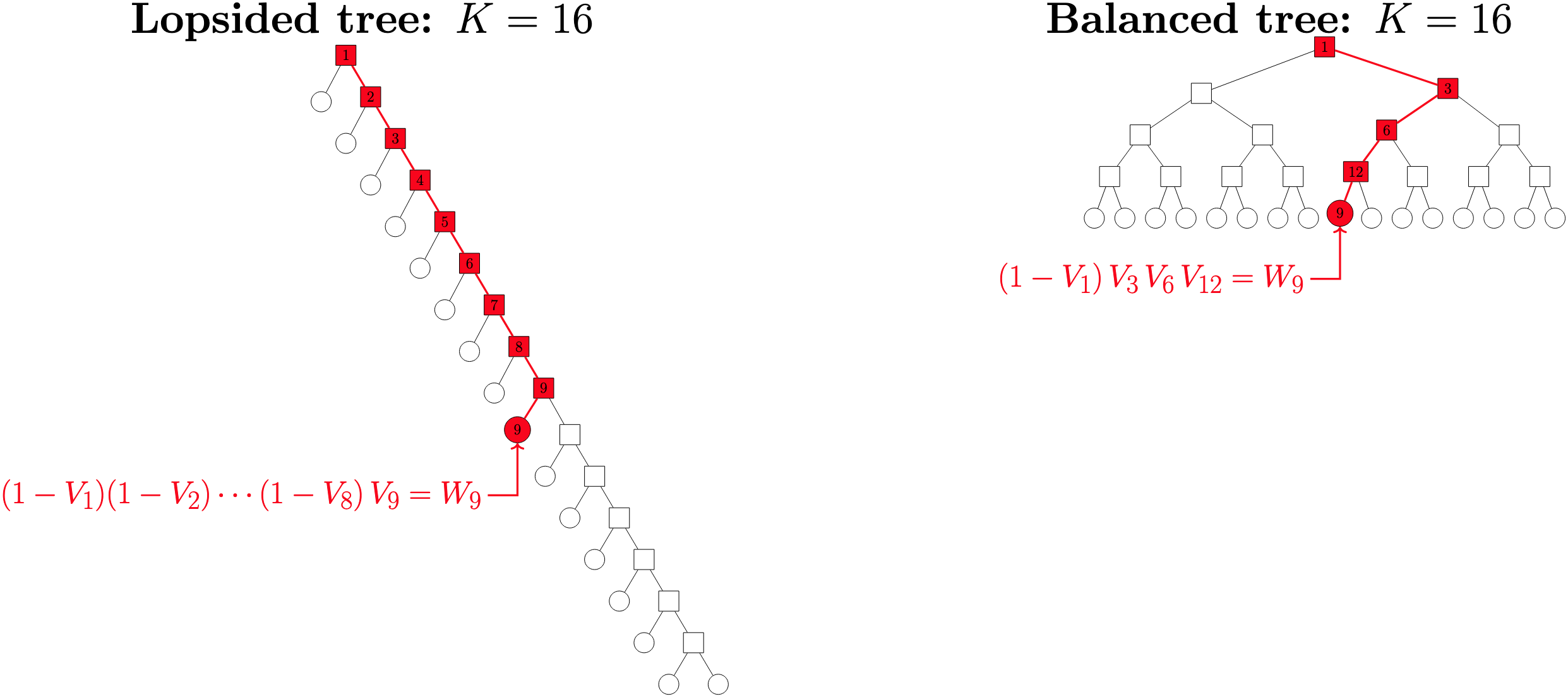
Figure 1: Binary tree representation of stick-breaking schemes. Each scheme’s initial stick break is represented as a root node; each subsequent stick break is represented by an internal node. The mass of a stick-break’s “left (right) piece” is sent to its left (right) child. The $K$ leaf nodes represent the scheme’s $K$ weights. As an example, weight $W_{9}$ is a product of nine stick breaks in the lopsided-tree scheme but only four stick breaks in the balanced-tree scheme.

More specifically, we show that in the context of covariate-dependent mixture modeling, which is a major field of application for stick-breaking models, common model specifications with a lopsided tree structure induce three undesirable characteristics that can severely deteriorate the quality of Bayesian inference in terms of increased posterior uncertainty and reduced computational efficiency. Some of these properties have been noted previously in the literature, but they were never attributed to the underlying lopsided tree structure, which we show is a major culprit. In addition we show through a combination of theoretical analysis, numerical experiments, and a case study that these three undesirable features of stick-breaking models can be resolved by simply adopting an alternative dyadic tree structure, namely a “balanced” tree (illustrated in Figure 1), corresponding to continually breaking off both remaining sticks at each stick-breaking step, without complicating the modeling and computational recipes that stick-breaking models enjoy.

What are these three undesirable characteristics of (lopsided-tree) stick-breaking processes in covariate-dependent mixture modeling? The first characteristic, which will be the focus of Section 3, is that under commonly adopted “default” specifications, covariate-dependent stick-breaking models can induce a strong positive prior correlation in the random measures over covariate values, which can cause excessive smoothing across the covariates even when the corresponding cluster sizes vary sharply across covariate values, thereby deprecating the clustering at each covariate value. This phenomenon was first explained in Rodríguez and Dunson (2011) in the context of probit-stick-breaking models as “a consequence of our use of a common set of atoms at every [covariate]; even if the set of weights are independent from each other, the fact that the atoms are shared means that the distributions cannot be independent.” Interestingly, we show this statement is true only if the weights are constructed by a lopsided tree-based stick-breaking, which leads to the effects of shared atoms on prior correlation.

The second characteristic, which will be the theme of Section 4, concerns the precision of the inference, in terms of the posterior uncertainty of covariate effects on mixing weights. Common prior specifications of covariate effects in stick-breaking weights introduce many competing mechanisms in a mixture model. In particular, stochastic ordering of the weights and the large number of stick breaks the weights is a product of (on average) introduce mechanisms that, at best, add unnecessary layers of complexity and, at worst, actively degrade the quality of posterior inference.

The third and final characteristic, which will be the focus of Section 5, concerns the Markov Chain Monte Carlo mixing and convergence and involves the phenomenon of component label switching (see Stephens, 2000; Papastamoulis, 2016, for an overview). In a Bayesian mixture model with $K$ components under a prior with exchangeable mixture components, the prior and the resulting posterior cannot distinguish the $K!$ permutations of the mixture component labels and hence are symmetric between the corresponding $K!$ regions of the parameter space (Rodríguez and Walker, 2014). Label switching, which is when a posterior sampler switches the labels of two components of a mixture model, has been observed to occur spontaneously in Markov chain Monte Carlo algorithms that use single-piece stick breaking (e.g. Redner and Walker, 1984; Celeux et al., 2000). Label switching hinders the interpretation of posterior inference results, and we find the common strategy of post-hoc relabeling (e.g. Cron and West, 2011) does not fully restore interpretation in all situations. Despite this, label switching moves are sometimes intentionally added to posterior inference algorithms (e.g. Frühwirth-Schnatter, 2001; Papaspiliopoulos and Roberts, 2008) because they are seen as a way to achieve convergence to the true posterior (Jasra et al., 2005). We show through numerical experiments that the frequency in which label switching occurs in Markov chain Monte Carlo sampling is influenced by underlying tree topology corresponding to the stick-breaking model. Moreover, for the chain to converge to the true posterior, it should explore all $K!$ regions of the parameter space. This can become an unattainable goal to pursue for even moderately large $K$. As an alternative, Puolamäki and Kaski (2009) suggest a chain can achieve the desired posterior inference by sufficiently exploring just a single region. The effectiveness of this alternative clearly depends on the extent to which the single region being explored is representative of the full posterior, which as we argue benefits from the symmetry in the prior probability assignment over the different cluster labeling and is also affected by the underlying tree topology corresponding to the stick-breaking model.

To finish the introduction, we relate to some relevant papers in the literature that involve tree-structured Bayesian nonparametric models. stick-breaking models over a general tree topology are closely related to tree-structured random measures such as the Pólya tree, and their generalizations involving covariate-dependence has a parallel development for tree-structured random measures, namely the covariate-dependent tail-free model introduced by Jara and Hanson (2011). To our knowledge, such processes have not been applied as a discrete prior for mixing distributions except in Cipolli and Hanson (2017) who propose the finite Pólya tree as a prior for the mixing distributions. Stefanucci and Canale (2021) introduce another weight-generating mechanism along a balanced bifurcating tree that includes stick-breaking models as special cases, but this generalization loses the main computational benefits of stick-breaking models in incorporating covariates. Finally, Ren et al. (2011) note a covariate-dependent stick-breaking process “may be viewed as a mixture-of-experts model” (Jordan and Jacobs, 1994; Peng et al., 1996; Bishop and Svensén, 2002) which uses a binary tree to define a covariate-dependent mixture distribution. Although we investigate the influence of the tree topology mainly in the context of stick-breaking models, the lessons drawn are also generally applicable to the context of mixture-of-experts models given the connection between the two model classes.

2 Stick-breaking models from a tree perspective

We start by introducing our tree-based stick-breaking construction in the absence of covariates and then extend the construction to include covariates. This broader class of models contains existing stick-breaking models as a special case corresponding to a particular lopsided tree topology. This will let us later examine the impact of the tree topology on Bayesian inference through the lens of comparing models within this broader class.

Throughout we assume independent and identically distributed (i.i.d.) observations $y_{1},\ldots,y_{n}\in\mathbb{R}^{d}$ from a sampling density of the mixture form $f(\cdot;G)=\int_{\Theta}h(\cdot;\theta)\mathop{}\!\mathrm{d}G(\theta)$, where $h\colon\mathbb{R}^{d}\times\Theta\rightarrow\mathbb{R}^{+}$ is a parametric mixing kernel density, e.g., Gaussian density $h(y;\theta)=(2\pi\sigma^{2})^{-1/2}\exp\left\{-(y-\mu)^{2}/(2\sigma^{2})\right\}$ with $\theta=(\mu,\sigma^{2})\in\mathbb{R}\times\mathbb{R}^{+}$.

If a mixing measure $G$ on $\Theta$ is equipped with a stick-breaking prior, each realization of $G$ is, with probability one, a discrete measure $G=\sum_{k=1}^{\infty}W_{k}\delta_{\theta_{k}}$ where the atoms $\theta_{k}$ are generated independently from a probability measure $G_{0}$ on $\Theta$ and the nonnegative weights $W_{k}$, which are generated by breaking a unit stick, are independent of the atoms $\theta_{k}$. This turns the mixture density $\int_{\Theta}h(\cdot;\theta)\mathop{}\!\mathrm{d}G(\theta)$ into the discrete sum $\sum_{k=1}^{\infty}W_{k}h(\cdot;\theta_{k})$.

The remainder of this section examines the traditional stick-breaking scheme from a tree perspective, and then introduces a tree-based generalization to stick-breaking priors.

2.1 Stick-breaking models without covariates

A weight-generation process aims to produce nonnegative quantities that sum to unity. A stick-breaking process achieves this by successively breaking off pieces of a stick of initially unit length, where the lengths of the resulting pieces become the desired weights. In traditional stick-breaking, each stick break produces a piece that is untouched afterwards while the other piece—the “remaining stick”—breaks again and again. More formally, to begin, a unit-length stick breaks at location $V_{1}\in[0,1]$ so that the piece that breaks off has length $V_{1}$. The remaining stick, of length $1-V_{1}$, then breaks at (relative) location $V_{2}\in[0,1]$ so that the new piece that breaks off has length $(1-V_{1})V_{2}$. The remaining stick, now of length $(1-V_{1})(1-V_{2})$, then breaks at location $V_{3}\in[0,1]$ so that the new piece that breaks off has length $(1-V_{1})(1-V_{2})V_{3}$, so on and so forth. For each $k\in\mathbb{N}$, the $k^{\text{th}}$ stick break at location $V_{k}\in[0,1]$ produces a piece that breaks off with length $V_{k}\prod_{l=1}^{k-1}(1-V_{l})$, which sets the value of weight $W_{k}$; the remaining stick then breaks at location $V_{k+1}\in[0,1]$. The process can either continue infinitely or terminate after a preset finite number of breaks, in which case the final remaining stick sets the last weight.

A stick-breaking scheme can be identified with a bifurcating tree whose nodes correspond to the pieces that arise during the stick breaking procedure. We construct the binary tree by first assigning the initial unit-length stick to the tree’s root node, and iteratively apply the following steps. If a piece of the stick does not break further, the piece corresponds to a leaf node, i.e., a node with no children. If a piece is further broken instead, the two resulting pieces correspond to two children nodes. The traditional stick-breaking scheme’s identified bifurcating tree (see the left of Figure 1) is the most “lopsided” as none of its nodes have children that both divide further. It is the deepest tree possible for generating a given number of pieces. We shall thus refer to the traditional stick-breaking strategy as lopsided-tree stick-breaking.

Given this tree view of stick-breaking, it is natural to consider stick-breaking schemes corresponding to binary tree topologies that differ from the lopsided one. To this end, it will be convenient to index the root node by the empty string $\emptyset$ and each other tree node $\bm{\varepsilon}$ by a finite string of 0s and 1s, where each digit indicates whether a node along the path from root to $\bm{\varepsilon}$ is a left (0) or right (1) child of its parent. In general, any node at level $m$ of the tree (the root node is at level 0, its two children are at level 1, and so on) is indexed by a $m$-length binary string $\varepsilon_{1}\varepsilon_{2}\cdots\varepsilon_{m}$, where the string $\bm{\varepsilon}\bm{\varepsilon}^{\prime}$ denotes the concatenation of finite strings $\bm{\varepsilon}$ and $\bm{\varepsilon}^{\prime}$. The set of all finite binary strings (including $\emptyset$) is denoted by $E^{*}\coloneqq\cup_{m=0}^{\infty}\{0,1\}^{m}$. This machinery allows us to formally introduce stick-breaking strategies based on general tree topologies.

We give particular attention to the stick-breaking scheme corresponding to a “balanced” bifurcating tree, in which all nodes (up to a maximum level) are split into two children as illustrated at the right of Figure 1. We refer to this stick-breaking scheme as a balanced-tree stick-breaking. Opposite of the lopsided-tree scheme, the balanced-tree scheme results in the most shallow tree topology needed to generate any given number of weights. In this scheme, each stick break produces two pieces that both break again until the total number of breaks exceeds a preset threshold (we argue against allowing infinitely many breaks in Section 2.2). More formally, the unit-length stick $I_{\emptyset}$ breaks according to $V_{\emptyset}$ so that the left piece $I_{0}$ has length $|I_{0}|=|I_{\emptyset}|V_{\emptyset}=V_{\emptyset}$ and the right piece has length $|I_{1}|=|I_{\emptyset}|(1-V_{\emptyset})=1-V_{\emptyset}$. These two pieces $I_{0}$ and $I_{1}$ then break similarly according to respective splitting variables $V_{0}$ and $V_{1}$ so that the resulting four pieces $I_{00}$, $I_{01}$, $I_{10}$, and $I_{11}$ have lengths $|I_{00}|=V_{\emptyset}V_{0}$, $|I_{01}|=V_{\emptyset}(1-V_{0})$, $|I_{10}|=(1-V_{\emptyset})V_{1}$, and $|I_{11}|=(1-V_{\emptyset})(1-V_{1})$. These four pieces then break similarly according to respective splitting variables $V_{00}$, $V_{01}$, $V_{10}$, and $V_{11}$ to produce the eight pieces $I_{000}$, $I_{001}$, $I_{010}$, $I_{011}$, $I_{100}$, $I_{101}$, $I_{110}$, and $I_{111}$ with lengths defined similarly. If each piece is only allowed to be a product of at most $m\in\mathbb{N}$ stick breaks, this recursive procedure produces $2^{m}$ leaf nodes each with a stick piece. The lengths of these pieces define the desired weights: $W_{\bm{\varepsilon}}\coloneqq|I_{\bm{\varepsilon}}|$ for each $\bm{\varepsilon}\in\{0,1\}^{m}$.

The value of any stick-breaking weight at a node $\bm{\varepsilon}=\varepsilon_{1}\cdots\varepsilon_{m}$ can be expressed as

$$W_{\varepsilon_{1}\cdots\varepsilon_{m}}=\prod_{l=1}^{m}V_{\varepsilon_{1}\cdots\varepsilon_{l-1}}^{1-\varepsilon_{l}}(1-V_{\varepsilon_{1}\cdots\varepsilon_{l-1}})^{\varepsilon_{l}}\quad\quad V_{\bm{\varepsilon}}\sim F_{\bm{\varepsilon}}\text{ for all }\bm{\varepsilon}\in E^{*}$$ (1)

where by convention $\varepsilon_{1}\cdots\varepsilon_{l-1}=\emptyset$ if $l=1$, and the splitting variables are distributed according to a countable sequence $\{F_{\bm{\varepsilon}}\colon\bm{\varepsilon}\in E^{*}\}$ of distributions each with full support on $[0,1]$ and the tail-free condition $V_{\emptyset}\perp\{V_{0},V_{1}\}\perp\{V_{00},V_{01},V_{10},V_{11}\}\perp\cdots$ (Freedman, 1963; Fabius, 1964).

We can now define the tree stick-breaking class of priors, which includes traditional stick-breaking and balanced-tree stick-breaking but also admits more general tree structures. We say a probability measure $G$ is endowed with a tree stick-breaking prior with parameters $G_{0}$, $\{F_{\bm{\varepsilon}}\}$, and binary tree structure $\tau$, denoted by $G\sim treeSB(G_{0},\{F_{\bm{\varepsilon}}\},\tau)$, if it can be constructed as

$$G=\sum_{\bm{\varepsilon}\in B(\tau)}W_{\bm{\varepsilon}}\delta_{\theta_{\bm{\varepsilon}}},\qquad\theta_{\bm{\varepsilon}}\stackrel{{\scriptstyle ind}}{{\sim}}G_{0}$$ (2)

where the set $B(\tau)\subset E^{*}$ indexes $\tau$’s leaf nodes, and the random weights $\{W_{\bm{\varepsilon}}\colon\bm{\varepsilon}\in B(\tau)\}$ are constructed according to (1) where the distributions $F_{\bm{\varepsilon}}$ follow the full-support and tail-free conditions. As with traditional stick-breaking, this turns the mixture density $\int_{\Theta}h(\cdot;\theta)\mathop{}\!\mathrm{d}G(\theta)$ into the discrete sum $\sum_{\bm{\varepsilon}\in B(\tau)}W_{\bm{\varepsilon}}h(\cdot;\theta_{\bm{\varepsilon}})$.

2.2 Choice of number of leaves

This section considers how should a practitioner should choose the number of leaves $K$ in the tree $\tau$ used in a tree stick-breaking prior. As $K\rightarrow\infty$, the tree stick-breaking prior ideally will increasingly resemble a well-defined Bayesian nonparametric prior that produces a discrete measure. Hence we first examine whether the tree stick-breaking prior can produce a discrete measure when $K=\infty$. The Dirichlet process is a well-known example of an infinitely deep lopsided tree that almost surely induces a discrete measure. For an infinitely deep balanced tree, Theorem 3.18 of Ghosal and van der Vaart (2017) states a tail-free process with splitting variables strictly between $0$ and $1$ is discrete with probability either zero or one; this probability is one if $V_{\bm{\varepsilon}}\stackrel{{\scriptstyle iid}}{{\sim}}\text{Be}(2^{-|\bm{\varepsilon}|},2^{-|\bm{\varepsilon}|})$ for all $\bm{\varepsilon}\in E^{*}$ (Ferguson, 1973).

We next explore which values of $K$ are appropriate. The posterior inference algorithm in Section 4 requires $K$ to be finite and not so large as to render computation intractable. On the other hand, $K$ should be large enough to capture the “true” number of clusters as well as sufficiently approximate the limiting Bayesian nonparametric prior. For a lopsided tree, the exponential bounds in the finite approximation theorems of Ishwaran and James (2002) imply the value of $K$ beyond say $64$ seems to affect inference by at most a trivial amount (assuming the “true” number of clusters is not greater than $64$). We introduce Theorem 1 below so that we can make a similar statement for a balanced tree. A rule of thumb that still allows “room to breathe” is to set $K$ to be the smallest power of two greater than or equal to twice the prior expected number of clusters.

Theorem 1.

Consider a sequence $\{\mathcal{T}_{j}=\{A_{\bm{\varepsilon}}:\bm{\varepsilon}\in\{0,1\}^{j}\}:j\in 0,1,2,\ldots\}$ of measurable partitions of the sample space obtained by splitting every set in the preceding partition into two new sets. Suppose $\text{diam}(A_{\bm{\varepsilon}})=2^{-|\bm{\varepsilon}|}$ for all $A_{\bm{\varepsilon}}$, where $|\bm{\varepsilon}|$ is the length of the string $\bm{\varepsilon}$ of 0s and 1s. If two tail-free processes agree on all subsets $A_{\bm{\varepsilon}}$ with $|\bm{\varepsilon}|\leq M$ for some positive integer $M$, then the Wasserstein distance between these two processes is bounded above by $2^{-M+1}$.

2.3 Tree stick-breaking with covariates

Following the well-known strategy of the unpublished 2000 technical report by S. N. MacEachern, we next extend the covariate-independent tree stick-breaking prior (2) by replacing the splitting variables $\{V_{\bm{\varepsilon}}\}_{\bm{\varepsilon}\in E^{*}}$ in (1) with a sequence of stochastic processes $\{V_{\mathbf{x},\bm{\varepsilon}}\colon\mathbf{x}\in\mathcal{X}\}_{\bm{\varepsilon}\in E^{*}}$, where $\mathcal{X}$ is a set of covariates and each splitting variable $V_{\mathbf{x},\bm{\varepsilon}}$ has distribution $F_{\mathbf{x},\bm{\varepsilon}}$. The resulting random measure $G_{\mathbf{x}}\sim treeSB(G_{0},\{F_{\mathbf{x},\bm{\varepsilon}}\},\tau)$ now depends on $\mathbf{x}$ through its weights: $G_{x}=\sum_{\bm{\varepsilon}\in B(\tau)}W_{\mathbf{x},\bm{\varepsilon}}\delta_{\theta_{\bm{\varepsilon}}}$ where $\theta_{\bm{\varepsilon}}\stackrel{{\scriptstyle ind}}{{\sim}}G_{0}$.

There are a number of possible strategies to incorporate covariate dependence on weights, including utilizing probit and logit transform on the weights as is commonly done for traditional stick-breaking. In particular, we consider the logit approach due to the computational convenience for posterior inference that follows from the Pólya-Gamma augmentation technique detailed in Section 4, though the theoretical properties we establish in Section 3.1 do not assume this model choice and apply more generally. Specifically, we adopt the following logit-normal model on each splitting variable:

$$V_{\mathbf{x},\bm{\varepsilon}}=\text{logistic}(\eta_{\mathbf{x},\bm{\varepsilon}}),\qquad\eta_{\mathbf{x},\bm{\varepsilon}}=\bm{\psi}(\mathbf{x})^{\top}\bm{\gamma}_{\bm{\varepsilon}},\qquad\bm{\gamma}_{\bm{\varepsilon}}\sim N_{R}(\bm{\mu}_{\bm{\gamma}},\bm{\Sigma}_{\bm{\gamma}})$$ (3)

with hyperparameters $\bm{\mu}_{\bm{\gamma}}$ and $\bm{\Sigma}_{\bm{\gamma}}$, where $\text{logistic}(z)=\exp\{z/(1+z)\}$ and $\eta_{\mathbf{x},\bm{\varepsilon}}$ is a linear combination of selected functions of the covariates $\bm{\psi}(\mathbf{x})=\{\psi_{1}(\mathbf{x}),\ldots,\psi_{R}(\mathbf{x})\}^{\top}$. Thus $\{\eta_{\mathbf{x},\bm{\varepsilon}}\colon\mathbf{x}\in\mathcal{X}\}$ is a Gaussian process with mean $\bm{\psi}(\mathbf{x})^{\top}\bm{\mu}_{\bm{\gamma}}$ and covariance $\texttt{Cov}(\eta_{\mathbf{x},\bm{\varepsilon}},\eta_{\mathbf{x}^{\prime},\bm{\varepsilon}})=\bm{\psi}(\mathbf{x})^{\top}\bm{\Sigma}_{\bm{\gamma}}\bm{\psi}(\mathbf{x}^{\prime})$. The remainder of the paper (except for Section 3.1) assumes the logit-normal prior (3).

3 Impact of the tree on cross-covariate correlation

This section examines the impact of tree topology on the prior cross-covariate correlation between two random measures created by stick breaking with dependent mixture weights and independent atoms. We provide expressions for various moments of the covariate-dependent random measures and create a simulation study that explores the cross-covariate correlation between random measures.

3.1 Moments of random measures

The prior (3) satisfies the conditions Theorems 2 and 3 place on the splitting variables.

Theorem 2.

Suppose for any covariates $\mathbf{x}$ that the random measure $G_{\mathbf{x}}=\sum_{k=1}^{K}W_{\mathbf{x},k}\,\delta_{\theta_{k}}$, with $K\in\{1,2,\ldots,\infty\}$, on $\Theta$ is constructed by drawing each $\theta_{k}$ independently (of each other and of $\mathbf{x}$) from some base measure $G_{0}$ on $\Theta$, and drawing a weight vector $(W_{\mathbf{x},1},\ldots,W_{\mathbf{x},K})$ according to some distribution (that might depend on $\mathbf{x}$) on the probability simplex $\Delta_{K}$.

For any measurable sets $A,A^{\prime}\in\mathcal{B}$ and covariates $\mathbf{x},\mathbf{x}^{\prime}$, we have

$$\mathbb{E}(G_{\mathbf{x}}(A)) =G_{0}(A)$$ (4)

$$\texttt{Var}(G_{\mathbf{x}}(A)) =\left\{G_{0}(A)-G_{0}^{2}(A)\right\}a_{\mathbf{x},\mathbf{x}}$$ (5)

$$\texttt{Cov}(G_{\mathbf{x}}(A),G_{\mathbf{x}}(A^{\prime})) =\left\{G_{0}(A\cap A^{\prime})-G_{0}(A)G_{0}(A^{\prime})\right\}a_{\mathbf{x},\mathbf{x}}$$ (6)

$$\texttt{Cov}(G_{\mathbf{x}}(A),G_{\mathbf{x}^{\prime}}(A)) =\left\{G_{0}(A)-G_{0}^{2}(A)\right\}a_{\mathbf{x},\mathbf{x}^{\prime}}$$ (7)

where $a_{\mathbf{x},\mathbf{x}^{\prime}}=\sum_{k=1}^{K}\mathbb{E}W_{\mathbf{x},k}W_{\mathbf{x}^{\prime},k}$. If also $G_{0}(A)\{1-G_{0}(A)\}G_{0}(A^{\prime})\{1-G_{0}(A^{\prime})\}\neq 0$, then

$$\texttt{corr}(G_{\mathbf{x}}(A),G_{\mathbf{x}}(A^{\prime})) =\frac{G_{0}(A\cap A^{\prime})-G_{0}(A)G_{0}(A^{\prime})}{\left[G_{0}(A)\{1-G_{0}(A)\}G_{0}(A^{\prime})\{1-G_{0}(A^{\prime})\}\right]^{1/2}}$$ (8)

$$\texttt{corr}(G_{\mathbf{x}}(A),G_{\mathbf{x}^{\prime}}(A)) =a_{\mathbf{x},\mathbf{x}^{\prime}}(a_{\mathbf{x},\mathbf{x}}a_{\mathbf{x}^{\prime},\mathbf{x}^{\prime}})^{-1/2}.$$ (9)

Per Theorem 2, each of these various moments factorizes into a function of the base measure $G_{0}$ and a function of the quantity $a_{\mathbf{x},\mathbf{x}^{\prime}}$. The mean (4) implies $G_{0}$ can be viewed as the mean of the random measure $G_{\mathbf{x}}$ while the correlation (8) does not depend on tree depth. On the other hand (and of greater interest), the cross-covariate correlation (9) depends not on the base measure $G_{0}$ but rather on $a_{\mathbf{x},\mathbf{x}^{\prime}}$, which Theorem 3 expresses as a function of $\tau$ and the splitting variables’ mean and cross-covariate covariance. In particular, this theorem states that $a_{\mathbf{x},\mathbf{x}^{\prime}}$ for a balanced tree approaches zero as $K\rightarrow\infty$ whereas $a_{\mathbf{x},\mathbf{x}^{\prime}}$ for a lopsided tree approaches a positive limit, which means a lopsided tree induces a baseline cross-covariate covariance value (7) between random measures that does not vanish as the number of weights approaches infinity. Corollary 3.1 states these statements also apply to their cross-covariate correlation counterparts (9) if the splitting variables have mean $1/2$ and nonnegative cross-covariate correlation.

Theorem 3.

Suppose weights $(W_{\mathbf{x},\bm{\varepsilon}}:\bm{\varepsilon}\in B(\tau))$ are constructed by stick-breaking according to tree topology $\tau$. Also assume that at any $\mathbf{x}$ the splitting variables $\{V_{\mathbf{x},\bm{\varepsilon}}:\bm{\varepsilon}\in E^{*}\}$ are identically distributed. Let $a_{\mathbf{x},\mathbf{x}^{\prime}}=\sum_{\bm{\varepsilon}\in B(\tau)}\mathbb{E}(W_{\mathbf{x},\bm{\varepsilon}}W_{\mathbf{x}^{\prime},\bm{\varepsilon}})$, where $B(\tau)$ is the set of $\tau$’s leaf nodes, and $K=|B(\tau)|\in\mathbb{N}$. If $\tau$ is a lopsided tree, then

$$a_{\mathbf{x},\mathbf{x}^{\prime}}=\frac{\mathbb{E}(V_{\mathbf{x}}V_{\mathbf{x}^{\prime}})\{1-[1-\mathbb{E}(V_{\mathbf{x}})-\mathbb{E}(V_{\mathbf{x}^{\prime}})+\mathbb{E}(V_{\mathbf{x}}V_{\mathbf{x}^{\prime}})]^{K}\}}{\mathbb{E}(V_{\mathbf{x}})+\mathbb{E}(V_{\mathbf{x}^{\prime}})-\mathbb{E}(V_{\mathbf{x}}V_{\mathbf{x}^{\prime}})}$$

which equals $\mathbb{E}(V_{\mathbf{x}}V_{\mathbf{x}^{\prime}})$ if $K=1$ and approaches $\{\mathbb{E}(V_{\mathbf{x}}V_{\mathbf{x}^{\prime}})\}/\{\mathbb{E}(V_{\mathbf{x}})+\mathbb{E}(V_{\mathbf{x}^{\prime}})-\mathbb{E}(V_{\mathbf{x}}V_{\mathbf{x}^{\prime}})\}$ as $K\rightarrow\infty$. If instead $\tau$ is a balanced tree and $m=\log_{2}K$, then

$$a_{\mathbf{x},\mathbf{x}^{\prime}}=\left\{1-\mathbb{E}(V_{\mathbf{x}})-\mathbb{E}(V_{\mathbf{x}^{\prime}})+2\mathbb{E}(V_{\mathbf{x}}V_{\mathbf{x}^{\prime}})\right\}^{m}$$

which approaches zero as $m\rightarrow\infty$.

Corollary 3.1 (Lower bounds).

If $\mathbb{E}(V_{\mathbf{x}})=1/2$ for any $\mathbf{x}$ and $\texttt{Cov}_{V}(\mathbf{x},\mathbf{x}^{\prime})\geq 0$ for any $\mathbf{x},\mathbf{x}^{\prime}\in\mathcal{X}$, lower bounds for (9) are $1/3$ for a lopsided tree and $2^{-m}$ for a balanced tree. These lower bounds are strict if $\texttt{Var}_{V}(\mathbf{x})>0$ for all $\mathbf{x}\in\mathcal{X}$.

Finally, the following theorem establishes the important property that the random measure $G_{\mathbf{x}}$ changes smoothly with respect to $\mathbf{x}$. This property requires a moment condition which is satisfied if the stochastic process $\{V_{\mathbf{x}}:\mathbf{x}\in\mathcal{X}\}$ is second-order stationary.

Theorem 4 (Smoothness).

Given the assumptions in Theorem 3, if $\mathbb{E}(V_{\mathbf{x}}V_{\mathbf{x}^{\prime}})\rightarrow\mathbb{E}(V_{\mathbf{x}}^{2})$ as $\mathbf{x}^{\prime}\rightarrow\mathbf{x}$, then (9) $\rightarrow 1$ as $\mathbf{x}^{\prime}\rightarrow\mathbf{x}$.

3.2 Numerical illustration on prior cross-covariate correlation

Here we explore the impact of the cross-covariate correlation between splitting variables on the cross-covariate correlation between random measures: given covariates $\mathbf{x}$ and $\mathbf{x}^{\prime}$, how does $\texttt{corr}(V_{\mathbf{x}},V_{\mathbf{x}^{\prime}})$ affect $\texttt{corr}\left(G_{\mathbf{x}}(A),G_{\mathbf{x}^{\prime}}(A)\right)$ for any measurable set $A\in\mathcal{B}$? We provide insight into this question through the following example.

Example 1.

We reduce the number of influences on $\texttt{corr}(V_{\mathbf{x}},V_{\mathbf{x}^{\prime}})$ by making the following assumptions: $\bm{\mu}_{\bm{\gamma}}=0_{2}$, $\bm{\Sigma}_{\bm{\gamma}}=\text{diag}(\sigma^{2}_{1},\sigma^{2}_{2})$, $\sigma^{2}_{1}>0$, $\bm{\psi}(\mathbf{x})=(1,0)^{\top}$, and $\bm{\psi}(\mathbf{x}^{\prime})=(1,1)^{\top}$. Though seemingly strict, these assumptions encompass a large class of scenarios. The mean-zero assumption is reasonable if no prior information is given. These assumptions also imply $\texttt{corr}(V_{\mathbf{x}},V_{\mathbf{x}^{\prime}})=\texttt{corr}(\eta_{\mathbf{x}},\eta_{\mathbf{x}^{\prime}})=(1+\tilde{\sigma}^{2}_{2})^{-1/2}$, which is a strictly decreasing function of $\tilde{\sigma}^{2}_{2}\coloneqq\sigma^{2}_{2}/\sigma^{2}_{1}\geq 0$ whose image is $(0,1]$. Thus, any positive value of $\texttt{corr}(V_{\mathbf{x}},V_{\mathbf{x}^{\prime}})$ can be achieved by using the appropriate $\tilde{\sigma}^{2}_{2}$ value if $\mathbf{x}\neq\mathbf{x}^{\prime}$. Similarly, these assumptions reduce $\texttt{corr}(G_{\mathbf{x}}(A),G_{\mathbf{x}^{\prime}}(A))$ (whose expression is provided by (9) and Theorem 3) to a function of $\sigma_{1}^{2}$, $\sigma_{2}^{2}$, $K$, and $\tau$.

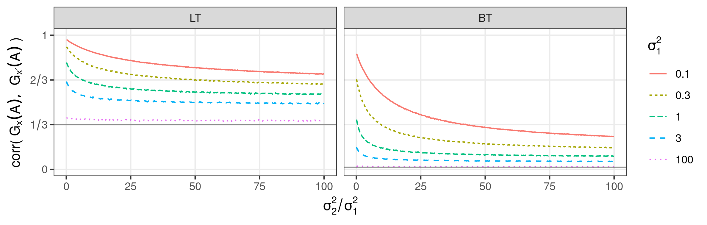
Figure 2: Simulated values of (9) as a function of $\tilde{\sigma}^{2}_{2}\coloneqq\sigma^{2}_{2}/\sigma^{2}_{1}$ for a lopsided and balanced tree each with $K=64$ and various values of $\sigma^{2}_{1}$. Lower bounds are shown as solid horizontal lines.

Figure 2 shows the behavior of $\texttt{corr}(G_{\mathbf{x}}(A),G_{\mathbf{x}^{\prime}}(A))$, which by Corollary 3.1 has lower bounds of $1/3$ and $1/K$ for, respectively, a lopsided tree and balanced tree. These lower bounds hold regardless of the degree of correlation between splitting variables, which in this scenario is controlled by choice of $\tilde{\sigma}^{2}_{2}$. Thus, the lopsided-tree scheme always imposes a nontrivial baseline correlation between random measures while the balanced-tree scheme can achieve both large and small correlation values, which provides more flexibility in setting prior correlation values.

4 Impact of the tree on posterior uncertainty

This section begins by detailing the posterior computation of the mixture model $f(\cdot;G_{\mathbf{x}})=\int_{\Theta}h(\cdot;\theta)\mathop{}\!\mathrm{d}G_{\mathbf{x}}(\theta)$ with a tree stick-breaking prior on the mixing measure $G_{\mathbf{x}}$. If $\tau$ is a lopsided tree with $K<\infty$ leaves, we call the resulting mixture a finite lopsided-tree mixture. We similarly define a finite balanced-tree mixture, where $K$ must be a power of $2$. This section then introduces a case study that analyzes flow-cytometry data and illustrates the impact of tree structure on the posterior uncertainty of covariate effects in mixture weights.

For posterior computation, we generalize Rigon and Durante (2021)’s Gibbs sampler to admit any stick-breaking scheme. Their Gibbs step for the regression coefficients $\bm{\gamma}$ relies on Polson et al. (2013)’s Pólya–Gamma data augmentation technique, which allows efficient posterior sampling of a Bayesian logistic regression. For this technique, Polson et al. (2013) carefully construct the Pólya–Gamma family of distributions to allow conditionally conjugate updating for the coefficient parameter and provide a fast, exact way to simulate Pólya–Gamma random variables. They show a posterior sampler for $\bm{\gamma}$ is obtained by iterating between a step that, conditional on $\bm{\gamma}$, samples the Pólya–Gamma data and a step that, conditional on the Pólya–Gamma data and regression responses, samples $\bm{\gamma}$ from a multivariate Gaussian distribution.

Result: Update each $R$-tuple $\bm{\gamma}_{\bm{\varepsilon}}$.

for each internal node $\bm{\varepsilon}$ in binary tree $\tau$ do

       Let $D_{\bm{\varepsilon}}$ be the set of indices $i\in\{1,\ldots,n\}$ where $C_{\tau}(i)$ is a descendant of node $\bm{\varepsilon}$ ;

       for every $i\in D_{\bm{\varepsilon}}$ do

             Sample Pólya-gamma data $[\omega_{i\bm{\varepsilon}}\mid\cdots]\sim\text{Pólya–gamma}(1,\,\bm{\psi}(\mathbf{x}_{i})^{\top}\bm{\gamma}_{\bm{\varepsilon}})$ ;

            

       end for

      Let $L_{\bm{\varepsilon}}\subset D_{\bm{\varepsilon}}$ be the set of indices corresponding to “left descendants” of node $\bm{\varepsilon}$ ;

       Update $\bm{\gamma}_{\bm{\varepsilon}}$ by drawing from full conditional

$$[\bm{\gamma}_{\bm{\varepsilon}}\mid\cdots]\sim N_{R}(\bm{\mu}_{\bm{\gamma}_{\bm{\varepsilon}}},\bm{\Sigma}_{\bm{\gamma}_{\bm{\varepsilon}}})$$

where, letting $\bm{\kappa}_{\bm{\varepsilon}}=(1_{i\in L_{\bm{\varepsilon}}}-0.5)_{i\in D_{\bm{\varepsilon}}}$ and $\mathbf{X}_{\bm{\varepsilon}}$ be the $|D_{\bm{\varepsilon}}|\times R$ matrix with row entries $\bm{\psi}(\mathbf{x}_{i})^{\top}$ for only those $i\in D_{\bm{\varepsilon}}$,

$$\bm{\mu}_{\bm{\gamma}_{\bm{\varepsilon}}}=\bm{\Sigma}_{\bm{\gamma}_{\bm{\varepsilon}}}\left[\mathbf{X}_{\bm{\varepsilon}}^{\top}\bm{\kappa}_{\bm{\varepsilon}}+\bm{\Sigma}_{\bm{\gamma}}^{-1}\bm{\mu}_{\bm{\gamma}}\right],\quad\bm{\Sigma}_{\bm{\gamma}_{\bm{\varepsilon}}}^{-1}=\mathbf{X}_{\bm{\varepsilon}}^{\top}\text{diag}(\omega_{1{\bm{\varepsilon}}},\ldots,\omega_{|D_{\bm{\varepsilon}}|\bm{\varepsilon}})\mathbf{X}_{\bm{\varepsilon}}+\bm{\Sigma}_{\bm{\gamma}}^{-1}.$$

end for

Algorithm 1 Gibbs step to update logit-normal coefficient under any binary tree.

Our generalization of this Gibbs step is stated explicitly in Algorithm 1. Given a posterior draw, for all $i=1,\ldots,n$ let $C_{\tau}(i)$ be $\tau$’s leaf node assigned to observation $i$. For each internal node $\bm{\varepsilon}$, the update for the coefficient $\bm{\gamma}_{\bm{\varepsilon}}$ relies on a Bayesian logistic regression with responses $Z_{i\bm{\varepsilon}}$, defined as the indicator that leaf node $C_{\tau}(i)$ is a “left descendant” of node $\bm{\varepsilon}$, for all $i$ corresponding to a descendant node of $\bm{\varepsilon}$. A “left descendant” of $\bm{\varepsilon}$ is either $\bm{\varepsilon}$’s left child or a descendant of $\bm{\varepsilon}$’s left child, and “right descendant” is defined similarly. In a lopsided tree the left child of any internal node is a leaf (see Figure 1) whereas for any internal node in a balanced tree the number of left descendants equals the number of right descendants. This formulation easily applies to any finite tree stick-breaking scheme. However, we find that training a balanced-tree mixture model takes less time than training its lopsided-tree counterpart for the data sets in Sections 4.1 and 5; this observation is supported by the theoretical discussion in Section 2 in the Supplementary Material.

For many applications, it is crucial to include random effects into the splitting-variable model. Without random effects, the model (3) makes the strong assumption that mixture-weight differences between groups is due entirely to differences in covariates. A mixture model that assumes (3) will resolve any large difference in cluster proportions between the two individuals that share the same covariates by breaking up the would-be cluster into many smaller clusters; such a mixture model would thus infer many more clusters than actually exists in the data (as we have seen from experience). Section 4.2 provides details of the specific random effects and the Gibbs sampler for a flow-cytometry case study, but these can easily generalize to other contexts.

4.1 The impact of the tree on posterior inference: a case study

We conduct a case study involving covariate-dependent clustering to demonstrate the influence of the tree topology on the posterior inference of the covariate effects over the cluster sizes. The scientific objective in this case study is to quantify the impact of an African-American female’s age on her proportions of T-cell types. Our analysis uses two groups of individuals, young (aged 18-29) and old (aged 50-65), from a publicly available data set to establish normative ranges (Yi et al., 2019) using the Human Immunology Profiling Consortium T cell immunophenotyping panel (Maecker et al., 2012). This panel has antibodies to cell surface proteins, known as markers, designed to identify CD4+ and CD8+ T cell activation and maturational status but is not specialized to resolve other immune cell types or degrees of immune senescence. The sample is of all peripheral blood mononuclear cells, and clusters may include non-T cell subsets. In standard analysis, an expert is required to visually identify distinct cell subsets using a sequence of 2D boundaries known as gates. We will instead identify cell subsets using a mixture model.

Our analysis is based on flow cytometry data measured on blood samples from 15 healthy plasma donors, six of which are 18-29 years old and remaining nine of which are 50-65 years old. Each sample can be roughly considered a collection of exchangeable observations (each corresponding to a blood cell) from a six-dimensional continuous sample space, with each dimension corresponding to the measurement from one marker. These 15 subjects together produce too many viable cells for the model to fit in a reasonable amount of time with Markov chain Monte Carlo. As such, we subset the data in a way that uses all 15 subjects while representing each age group by the same number of viable cells. Hence we subset a total of $n=403200$ viable cells where each age group is represented by $n/2$ cells. Within each age group, each subject contributes the same number of cells, i.e. the six 18-29 subjects each contributes one-sixth of the $n/2$ cells and the nine 50-65 subjects each contributes one-ninth of the $n/2$ cells.

4.2 A mixed-effects model and a recipe for Bayesian computation

In this study, cells are grouped by the subject they come from and subjects are grouped by the laboratory in which their cells are collected. We account for any resulting group effects in the mixture weights by including random effects in the splitting variables. For each subject $s$, each splitting variable will include fixed effects $\bm{\gamma}$ for covariates $\bm{\psi}(\mathbf{x}_{s})=(1,\text{age group of subject }s)^{\top}$, a random effect $u_{s}$ for the subject, and a random effect $v_{j}$ for the subject’s batch $j$ (we omit $j$’s dependence on $s$ to avoid visual clutter):

$$\text{logit }V_{s,\varepsilon} =\bm{\psi}(\mathbf{x}_{s})^{\top}\bm{\gamma}_{\varepsilon}+v_{j,\varepsilon}+u_{s,\varepsilon}.$$ (10)

The covariates and fixed effects are treated as in (3), and the random effects have priors

$$v_{j,\varepsilon}|\phi_{\varepsilon}^{(v)}\stackrel{{\scriptstyle ind}}{{\sim}}\text{N}(0,(\phi_{\varepsilon}^{(v)})^{-1}),\quad u_{s,\varepsilon}|\phi_{\varepsilon}^{(u)}\stackrel{{\scriptstyle ind}}{{\sim}}\text{N}(0,(\phi_{\varepsilon}^{(u)})^{-1}),\quad\phi_{\varepsilon}^{(v)},\phi_{\varepsilon}^{(u)}\stackrel{{\scriptstyle ind}}{{\sim}}\text{Gamma}(1,1).$$

Using Wang and Roy (2018)’s two-block Gibbs sampler, Algorithm 2 extends our Gibbs step from Algorithm 1 to also update the random effects.

Result: Update each fixed-effects $R$-tuple $\bm{\gamma}_{\bm{\varepsilon}}$ and random-effects $(J+S)$-tuple $\mathbf{u}_{\bm{\varepsilon}}$.

for each internal node $\bm{\varepsilon}$ in binary tree $\tau$ do

       Let $\mathcal{D}_{\bm{\varepsilon}}\subseteq\{1,\ldots,n\}$ be the set of indices $i$ where $C_{\tau}(i)$ is a descendant of node $\bm{\varepsilon}$ ;

       Update precision parameter $[\phi_{\bm{\varepsilon}}^{(v)}\mid\cdots]\sim\Gamma(a_{\bm{\varepsilon}}^{(v)}+0.5,b_{\bm{\varepsilon}}^{(v)}+0.5\sum_{j\in\mathcal{J}_{\bm{\varepsilon}}}v_{j,\bm{\varepsilon}}^{2})$, where $\mathcal{J}_{\bm{\varepsilon}}\subseteq\mathcal{J}$ is the set of batches corresponding to observations in $\mathcal{D}_{\bm{\varepsilon}}$ ;

       Update precision parameter $[\phi_{\bm{\varepsilon}}^{(u)}\mid\cdots]\sim\Gamma(a_{\bm{\varepsilon}}^{(u)}+0.5,b_{\bm{\varepsilon}}^{(u)}+0.5\sum_{s\in\mathcal{S}_{\bm{\varepsilon}}}u_{s,\bm{\varepsilon}}^{2})$, where $\mathcal{S}_{\bm{\varepsilon}}\subseteq\mathcal{S}$ is the set of subjects corresponding to observations in $\mathcal{D}_{\bm{\varepsilon}}$ ;

       for every observation $i\in\mathcal{D}_{\bm{\varepsilon}}$ do

             Sample $[\omega_{i\bm{\varepsilon}}\mid\cdots]\sim\text{Pólya–gamma}(1,\,|\bm{\psi}(\mathbf{x}_{s})^{\top}\bm{\gamma}_{\varepsilon}+u_{s,\varepsilon}+v_{j,\varepsilon}|)$, for the subject $s$ and batch $j$ associated with $i$ ;

            

       end for

      Let $\mathcal{L}_{\bm{\varepsilon}}\subset\mathcal{D}_{\bm{\varepsilon}}$ be the set of indices corresponding to left descendants of node $\bm{\varepsilon}$ ;

       Update fixed and random effects by drawing from the full conditional

$$\left[\begin{pmatrix}\bm{\gamma}_{\bm{\varepsilon}}\\ \mathbf{u}_{\bm{\varepsilon}}\end{pmatrix}\mid\cdots\right]\sim\text{N}_{R+J+S}(\bm{\mu}_{\bm{\gamma}_{\bm{\varepsilon}},\mathbf{u}_{\bm{\varepsilon}}},\bm{\Sigma}_{\bm{\gamma}_{\bm{\varepsilon}},\mathbf{u}_{\bm{\varepsilon}}})$$

where, letting $\mathbf{M}_{\bm{\varepsilon}}$ be the $|\mathcal{D}_{\bm{\varepsilon}}|\times(R+J+S)$ matrix with row entries $(\bm{\psi}(\mathbf{x}_{i})^{\top},\mathbf{z}_{i}^{\top})$ for only those $i\in\mathcal{D}_{\bm{\varepsilon}}$, $\bm{\kappa}_{\bm{\varepsilon}}=(1_{i\in\mathcal{L}_{\bm{\varepsilon}}}-0.5)_{i\in\mathcal{D}_{\bm{\varepsilon}}}$, $\bm{\Omega}_{\bm{\varepsilon}}=\text{diag}(\omega_{i{\bm{\varepsilon}}}:i\in\mathcal{D}_{\bm{\varepsilon}})$, and $\bm{\Phi}_{\bm{\varepsilon}}=(\phi_{\bm{\varepsilon}}^{(v)}\mathbf{I}_{J})\oplus(\phi_{\bm{\varepsilon}}^{(u)}\mathbf{I}_{S})$,

$$\bm{\mu}_{\bm{\gamma}_{\bm{\varepsilon}},\mathbf{u}_{\bm{\varepsilon}}}=\bm{\Sigma}_{\bm{\gamma}_{\bm{\varepsilon}},\mathbf{u}_{\bm{\varepsilon}}}\left[\mathbf{M}_{\bm{\varepsilon}}^{\top}\bm{\kappa}_{\bm{\varepsilon}}+\begin{pmatrix}\bm{\Sigma}_{\bm{\gamma}}^{-1}\bm{\mu}_{\bm{\gamma}}\\ 0_{(S+J)\times 1}\end{pmatrix}\right],\quad\bm{\Sigma}_{\bm{\gamma}_{\bm{\varepsilon}},\mathbf{u}_{\bm{\varepsilon}}}^{-1}=\mathbf{M}_{\bm{\varepsilon}}^{\top}\bm{\Omega}_{\bm{\varepsilon}}\mathbf{M}_{\bm{\varepsilon}}+(\bm{\Sigma}_{\bm{\gamma}}^{-1}\oplus\bm{\Phi}_{\bm{\varepsilon}}).$$

end for

Algorithm 2 Gibbs step to update fixed and random effects under any binary tree.

To the data we fit a lopsided-tree mixture model and a balanced-tree mixture model each with hyperparameter values of $K=16$, prior mean $\bm{\mu}_{\gamma}=0_{R}$, and prior covariance $\bm{\Sigma}_{\gamma}=10I_{R}$ where $R=7$. Each chain burns in $5000$ steps before sampling every $10$ steps to ultimately keep $1000$ posterior draws. Both models use cross-sample calibration to account for subject-data being collected in different batches (Gorsky et al., 2023).

4.3 Posterior summaries of the covariate effects on mixing weights

Because our scientific interest concerns the general African-American female population rather than only the subjects in our study, population-level parameters such as the effects of age should retain nontrivial posterior uncertainties due to the relatively small number of subjects in the study. Hence the effects of the study’s subjects on the mixture weights should be captured by the mixture model but the covariate effects on the cluster sizes should only be quantified by the difference in mixture weights across covariates at the population level, not for the specific individuals in the study. We compute this population-level weight difference by first fitting a mixture model with the mixed-effects model (10). Then we compute a population-level splitting variable $V_{s,\bm{\varepsilon}}^{*}$ for each subject $s$ and internal node $\bm{\varepsilon}$ using the posterior draws of only the covariate fixed effects, which per (10) implies $V_{s,\bm{\varepsilon}}^{*}$ depends on $s$ only through $s$’s age group $x_{s}\in\{old,young\}$ and hence can be written as $V_{x_{s},\bm{\varepsilon}}^{*}$. For each age group $x$, we convert $x$’s splitting variables into population-level mixture weights $\mathbf{W}_{x}^{*}\coloneqq(W_{x,\bm{\varepsilon}_{1}}^{*},\ldots,W_{x,\bm{\varepsilon}_{K}}^{*})\in\Delta_{K}$ using the usual tree-dependent conversion (1). We can then measure the age effect on the mixture weights at the population level as

$$\mathbf{W}_{old}^{*}-\mathbf{W}_{young}^{*}.$$ (11)

4.4 The influence of the tree topology on posterior inference

After fitting the mix-effects mixture model under both a lopsided tree and a balanced tree, we compare the inference between the corresponding posterior distributions. The two models infer very similar sample-level cluster sizes and shapes, see Figure 2 in the Supplemental Material, which indicates a degree of robustness in the inference and creates an approximate one-to-one correspondence between most of the lopsided-tree clusters and most of the balanced-tree clusters. This robustness in inferring sample-level cluster sizes and shapes, i.e., those for the specific samples collected in the study, are expected for flow cytometry given the massive number of cells in each sample. The difference in the lopsided-tree mixture and balanced-tree mixture is expected to be apparent on the population-level cluster sizes given the limited number of samples and the substantial sample-to-sample variability typically observed in flow cytometry.

Interesting differences show up in the posterior distributions of population-level parameters such as the covariate effects on cluster sizes. Given the approximate correspondence in the sample-level clusters, we can directly compare the inference on covariate effects (which are on the population-level cluster sizes) between the two models. Figure 3 shows both sets of credible intervals of (11) on each cluster in order of cluster size, which allows easier visual comparison between corresponding lopsided-tree and balanced-tree clusters. Even for cluster pairs with very similar size and shape, some of the corresponding credible intervals are noticeably different. In particular, consider the three cluster pairs whose $90\%$ credible intervals are most away from zero. For one of these three cluster pairs (whose size is roughly $7.1\%$ and whose biomarker values align with activated monocytes), the two credible intervals are similar in length but differ in location. For the remaining two cluster pairs (whose sizes are roughly $15.5\%$ and $2.8\%$ and whose biomarker values respectively align with those of CD4+ naïve T cells and resting monocytes), the balanced-tree credible intervals have smaller skewness and spread than do the lopsided-tree credible intervals. Regarding CD4+ naïve T cells, CD4+ T cells generally coordinate the overall immune response by the secretion of signaling molecules, and naïve T cells are cells which have never previously encountered antigen but might become memory cells after encountering antigen. Hence it is highly plausible that naïve T cells would decrease with age as their production slows down markedly after adolescence (Mogilenko et al., 2022), as suggested by the two credible intervals of this cluster.

Why these credible intervals are so different is difficult to pinpoint exactly due to the many moving parts in a mixture model, but we can offer a few conjectures. For example, consider the prior assumption of mean-zero covariate effects in the splitting variables. For either tree, it pushes clusters with strong covariate effects toward leaf nodes graphically near other because such a configuration would allow more splitting variables to maintain (near) zero-valued covariate effects. For this same reason, it also pushes such clusters away from the tree’s root. But for the lopsided-tree mixture model, prior stochastic ordering in the mixture weights pushes larger clusters toward the root and hence competes with the previous mechanism over large clusters with strong covariate effects (such as the cluster whose size is roughly $15.5\%$). In addition, for a mixture model with $K$ components, the lopsided-tree weights are on average a product of $\approx K/2$ splitting variables whereas each balanced-tree weight is a product of $\log_{2}K$ splitting variables, which implies the lopsided-tree weights are a more interdependent function of the splitting variables than are the balanced-tree weights. The exact way these mechanisms affect the quality of the posterior inference is unclear, but the seemingly fewer moving parts and more efficient model representation of the mixture weights in the balanced-tree mixture model are appealing.

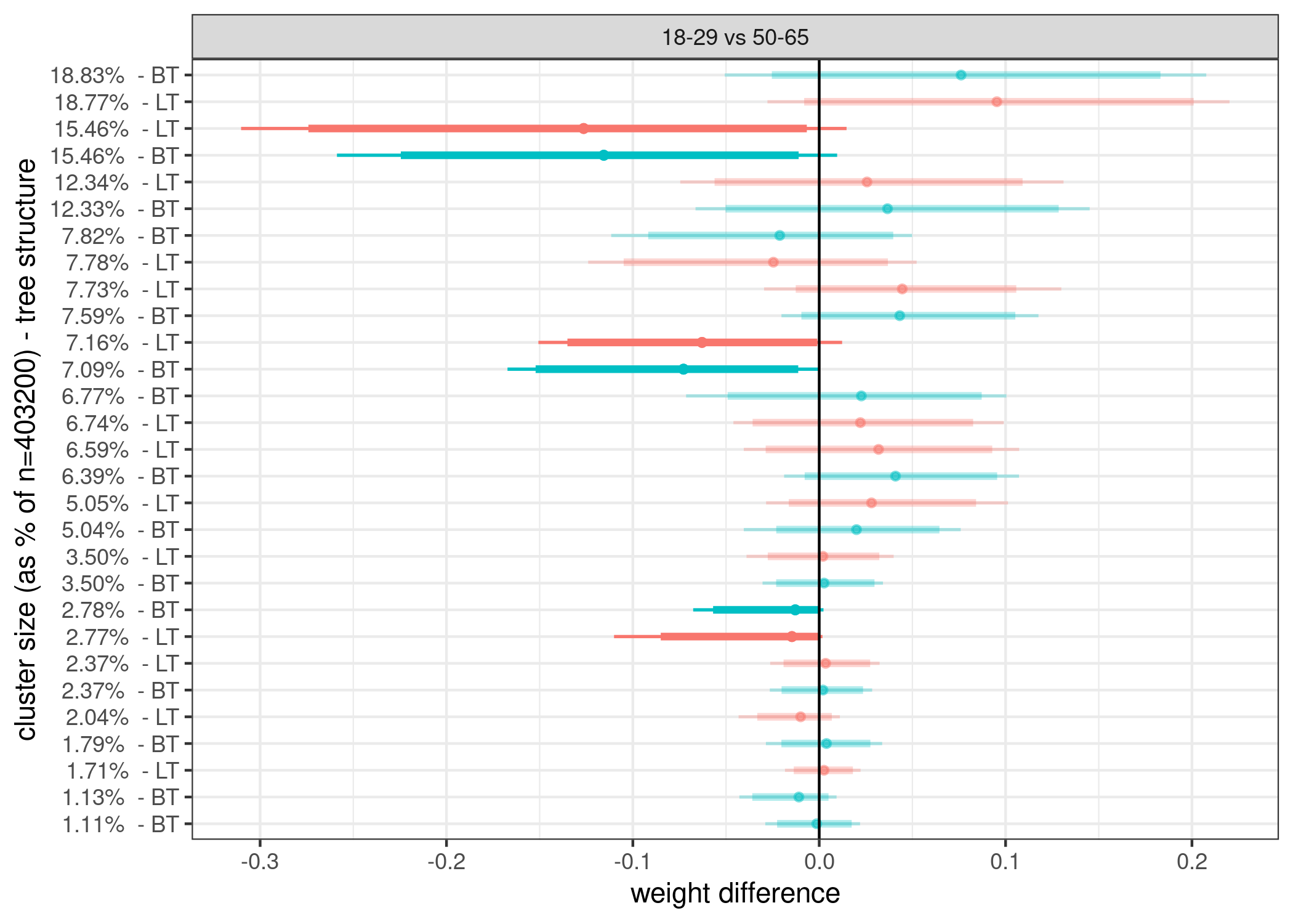
Figure 3: Credible intervals of (11) for both the fitted lopsided-tree mixture and balanced-tree mixture model. Thicker bar indicates $90\%$ quantile and thinner bar indicates $95\%$ quantile.

5 Impact of the tree on Markov chain Monte Carlo sampling

Label switching has been observed to occur frequently in Markov chain Monte Carlo algorithms for mixture models that use standard, or lopsided-tree, stick-breaking models. Despite label switching being seen as a way to achieve convergence to the true posterior, such convergence can often become an unattainable goal to pursue. In this section we design a simulation experiment to compare the frequency of label switching under stick-breaking models with different tree topologies. In particular, our results indicate that label switching can occur more often and to greater effect in the trained lopsided-tree mixture model than in the trained balanced-tree mixture model. We also discuss reasons behind this phenomenon.

We generate $n=$8000$$ observations each from one of 20 skew-normal distributions shown in Figure 3 of the Supplementary Material; these cluster counts are listed as the $20$-tuple $8\cdot(200,170,130,100,80,70,50,30,28,22,20,18,16,14,12,10,9,8,7,6)$. For each cluster, the observations are evenly assigned one of the eight covariates in the set $\{1\}\times\{0,1\}^{3}$. To the data we fit a lopsided-tree mixture model and a balanced-tree mixture model using the Gibbs step in Algorithm 1 with $K=32$, prior mean $\bm{\mu}_{\gamma}=0_{4}$, and prior covariance $\bm{\Sigma}_{\gamma}=10I_{4}$. Each chain burns in $100000$ steps before sampling every $100$ steps to keep $10000$ posterior draws.

Figure 4 in the Supplementary Material shows the Jaccard distance between each chain’s clustering at the $j$th posterior draw (for all $j=1,\ldots,$10000$$) and the true clustering (Jaccard, 1912). This distance provide a sense of a chain’s clustering performance and its mixing behavior. The two models have roughly the same median Jaccard distance of $0.043$, but the mean Jaccard distance is slightly larger for the lopsided-tree mixture model ($0.048$ vs $0.045$). The lopsided-tree chain also seems to get stuck in local modes for longer than the balanced-tree chain does.

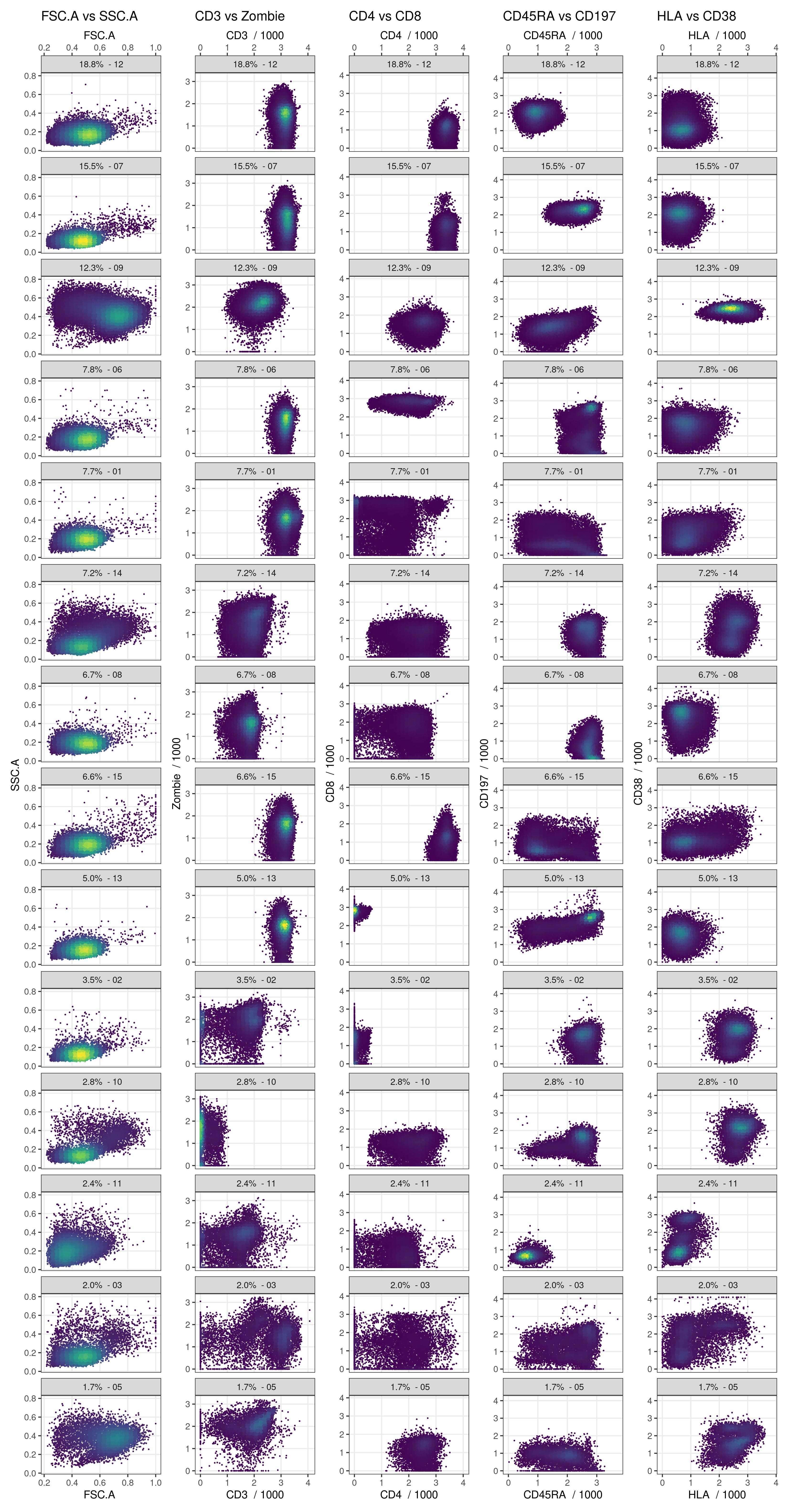
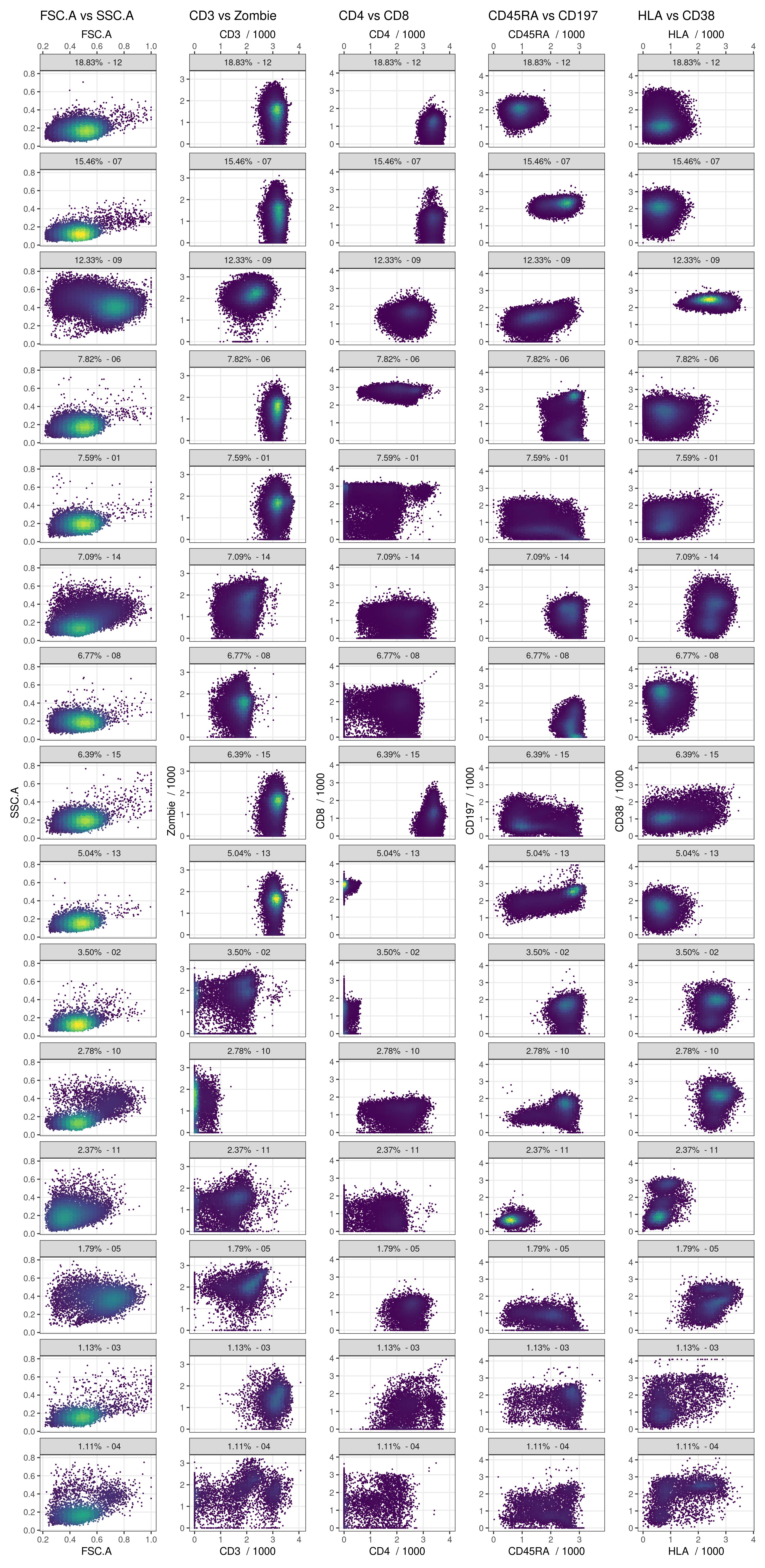
Figure 6: Clusters inferred by the lopsided-tree mixture model (left) and the balanced-tree mixture model (right).

What accounts for this difference in clustering behavior? Figure 4 shows selected mixture-weight inference for the covariate combination $1010$. The results are similar for the other covariate values as shown in Figure 5 in the Supplementary Material. In Figure 4(a)’s lopsided-tree panel, no credible interval is centered around the second largest weight value of $0.17$, which might foster the belief that this lopsided-tree mixture model fails to capture this weight, but the heights of the eight curiously wide $95\%$ credible intervals are roughly that same value. This observation together with Figure 4(b) imply the eight wide lopsided-tree credible intervals are a result of label switching in the Markov chain. Similarly, Figure 6a in the Supplemental Material implies the wide credible intervals in Figure 4(a)’s balanced-tree panel are also a result of label switching. Indeed, Figure 6c in the Supplemental Material shows these wide credible intervals disappear and the data’s weights are captured if we “resolve” the label switching by performing the following post-hoc sorting of weights: for each posterior draw $j$ we rearrange (in decreasing order) the elements of the chain’s corresponding weight vector $w_{1010}^{(j)}$, then for each newly rearranged weight index $\tilde{k}$ we compute credible intervals for the values in the set $\{w_{1010,\tilde{k}}^{(j)}:j=1,\ldots,$10000$\}$.

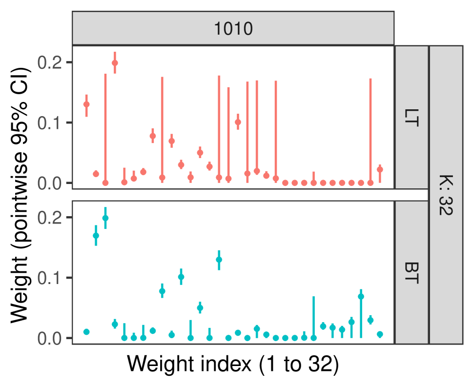
(a) Pointwise $95\%$ credible intervals of weights inferred by models trained on the two data sets.

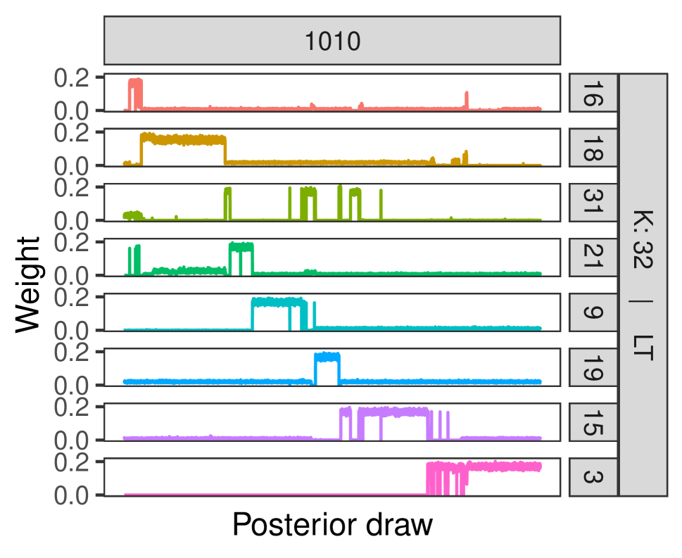
(b) Weights inferred by the lopsided-tree mixture for indices corresponding to wide credible intervals.

Figure 4: Selected mixture-weight inference for the covariate vector $1010$.

Although this post-hoc sorting seems to resolve the wide credible intervals for this example, the procedure requires several assumptions to work and hence cannot be applied generally. Until a general solution is created, it seems prudent to “nip the problem in the bud” by mitigating the impact of label switching on inference. But why does label switching seem to affect the lopsided-tree mixture’s inference more than balanced-tree mixture’s? We conjecture that the behavior difference stems from two tree-related mechanisms.

First, consider how much friction there is to label switch between two leaf nodes for either tree structure. The amount of friction seems to increase with the number of splitting variables affected by the proposed switch. If the two leaves are graphically far apart, the proposed switch would affect many splitting variables and hence be unlikely to occur. Under this reasoning, switching is most likely to occur between two leaves graphically near each other. In a balanced tree, this means two leaves that share the same parent. In a lopsided tree, this means two leaves separated by at most one tree level. For conceptual simplicity, we consider only such pairs and call these leaves adjacent to each other. Because a lopsided tree has $K-1$ adjacent pairs whereas a balanced tree has $K/2$, a lopsided tree has more adjacent pairs from which switching can occur.

Second, a label switch between two adjacent lopsided-tree leaves can create a “chain reaction” of label switches either up or down the entire tree. If a switch occurs between adjacent lopsided-tree leaf-pair $(\varepsilon 0,\varepsilon 10)$ for some internal node $\varepsilon$, the adjacent pair $(\varepsilon 10,\varepsilon 110)$ becomes “newly eligible” for switching, and if that switch eventually occurs, the adjacent pair $(\varepsilon 110,\varepsilon 1110)$ becomes “newly eligible” for switching, and so on, which creates the possibility of a chain reaction in the direction of increasing tree level (though a chain reaction can just as easily occur in the other tree direction). This might explain the behavior in Figure 4(b), where the $0.17$ mass moves almost sequentially through eight nodes. In contrast, because any balanced-tree leaf is adjacent to exactly one other leaf and because adjacency is a symmetric binary relation, any switch between two adjacent balanced-tree leaves will likely stay localized i.e. such a switch will likely not create any “newly eligible” pairs. This balanced-tree conjecture is supported by the chain behavior in Figure 6a in the Supplementary Material.

These two proposed mechanisms seem to explain the observed Markov chain Monte Carlo behavior difference between a lopsided tree and a balanced tree. Overall, our aforementioned inference observations indicate that if we consider the parameter space $\Theta$ and posterior local modes corresponding to label permutations, the regions between these local modes appear to be deeper valleys for the balanced-tree posterior than they are for the lopsided-tree posterior, making it more difficult to jump between different labelings for a balanced tree than for a lopsided tree.

6 Discussion

One limitation of the balanced tree model investigated in this work is that we assumed the tree is truncated at a maximum depth. With a sufficiently large depth this causes little practical restriction in applications, but it does preclude theoretical analysis of such models as fully nonparametric processes with infinite-dimensional parameters. Such an extension is of future interest. Another area of future work is to explore posterior-inference algorithms that avoid finite-dimensional approximations, allow covariates to be incorporated into mixture weights, and are computationally tractable. A Pólya-urn sampler is one such method of avoiding finite-dimensional approximations, but it is not clear if such an approach could be extended to incorporate covariate dependence. On the other hand, Foti and Williamson (2012) introduces a slice sampler for the dependent Dirichlet process which perhaps could be modified for a dependent balanced-tree mixture model.

Software

Our R package treeSB is available at https://github.com/ahoriguchi/treeSB. Code for our numerical examples is available at https://github.com/ahoriguchi/treeSB_Numerical_Examples.

SUPPLEMENTARY MATERIAL

Proofs:

Proofs of Theorems 1, 2, 3, and Corollary 2.1. (.pdf type)

Discussion:

Discussion on computational cost of Gibbs step from Algorithm 1. (.pdf type)

7 Proofs

7.1 Proof of Theorem 1

Proof of Theorem 1.

We use the following formulation of the Wasserstein distance of any two probability measures $P$ and $Q$ over the same measurable space:

$$W(P,Q)=\sup_{f\,1-Lip}\Bigg{\{}\int fdP-\int fdQ\Bigg{\}}.$$

where the supremum is over 1-Lipschitz functions $f$.

Now let $P$ and $Q$ be the two tail-free processes assumed in the theorem statement. Using any tree partition $\mathcal{T}_{j}$, the difference $\int fdP-\int fdQ$ can be decomposed into the sum $\sum_{A_{\bm{\varepsilon}}\in\mathcal{T}_{j}}[\int_{A_{\bm{\varepsilon}}}fdP-\int_{A_{\bm{\varepsilon}}}fdQ]$. Consider a single term in this sum. For any 1-Lipschitz function $f$ and any subset $A_{\bm{\varepsilon}}$ from any $\mathcal{T}_{j}$, define $\bar{f}_{\bm{\varepsilon}}=\int_{A_{\bm{\varepsilon}}}fd\mu/\mu(A_{\bm{\varepsilon}})$ where $\mu$ is the Lebesgue measure. Then the triangle inequality implies

$$\Bigg{|}\int_{A_{\bm{\varepsilon}}}fdP-\int_{A_{\bm{\varepsilon}}}fdQ\Bigg{|} \leq\Bigg{|}\int_{A_{\bm{\varepsilon}}}\bar{f}_{\bm{\varepsilon}}dP-\int_{A_{\bm{\varepsilon}}}\bar{f}_{\bm{\varepsilon}}dQ\Bigg{|}+\Bigg{|}\int_{A_{\bm{\varepsilon}}}(f-\bar{f}_{\bm{\varepsilon}})dP\Bigg{|}+\Bigg{|}\int_{A_{\bm{\varepsilon}}}(f-\bar{f}_{\bm{\varepsilon}})dQ\Bigg{|}$$

$$\leq\bar{f}_{\bm{\varepsilon}}\big{|}P(A_{\bm{\varepsilon}})-Q(A_{\bm{\varepsilon}})\big{|}+\text{diam}(A_{\bm{\varepsilon}})\big{[}P(A_{\bm{\varepsilon}})+Q(A_{\bm{\varepsilon}})\big{]},$$

where $\text{diam}(A_{\bm{\varepsilon}})=2^{-|\bm{\varepsilon}|}$ by assumption. If $|\bm{\varepsilon}|\leq M$, then $P(A_{\bm{\varepsilon}})=Q(A_{\bm{\varepsilon}})$ by assumption, which makes the preceding bound equal to $P(A_{\bm{\varepsilon}})2^{-|\bm{\varepsilon}|+1}$. So if we decompose $\int fdP-\int fdQ$ using the tree partition $\mathcal{T}_{M}$, we get

$$W(P,Q)\leq\sum_{A_{\bm{\varepsilon}}\in\mathcal{T}_{M}}P(A_{\bm{\varepsilon}})2^{-M+1}=2^{-M+1}.$$

∎

7.2 Proof of Theorem 2

Proof of Theorem 2.

This proof follows closely from Appendix 2 of Rodríguez and Dunson (2011). To prove the mean result (8), we have

$$\mathbb{E}\{G_{\mathbf{x}}(A)\} =\mathbb{E}\left\{\sum_{k=1}^{K}W_{\mathbf{x},k}\delta_{\theta_{k}}(A)\right\}=\sum_{k=1}^{K}\mathbb{E}(W_{\mathbf{x},k})\text{pr}(\theta_{1}\in A)=G_{0}(A).$$

To prove the remaining results, let $X=G_{\mathbf{x}}(A)$ and $Y=G_{\mathbf{x}^{\prime}}(A^{\prime})$ and note

$$\mathbb{E}(XY) =\mathbb{E}\left[\left\{\sum_{k=1}^{K}W_{\mathbf{x},k}\delta_{\theta_{k}}(A)\right\}\left\{\sum_{k=1}^{K}W_{\mathbf{x}^{\prime},k}\delta_{\theta_{k}}(A^{\prime})\right\}\right]$$

$$=\sum_{k=1}^{K}\mathbb{E}\left\{W_{\mathbf{x},k}W_{\mathbf{x}^{\prime},k}\delta_{\theta_{k}}(A)\delta_{\theta_{k}}(A^{\prime})\right\}+\sum_{k=1}^{K}\sum_{k^{\prime}\neq k}\mathbb{E}\left\{W_{\mathbf{x},k}W_{\mathbf{x}^{\prime},k^{\prime}}\delta_{\theta_{k}}(A)\delta_{\theta_{k^{\prime}}}(A^{\prime})\right\}$$

$$=G_{0}(A\cap A^{\prime})a_{\mathbf{x},\mathbf{x}^{\prime}}+G_{0}(A)G_{0}(A^{\prime})b_{\mathbf{x},\mathbf{x}^{\prime}}$$

where $a_{\mathbf{x},\mathbf{x}^{\prime}}=\sum_{k=1}^{K}\mathbb{E}(W_{\mathbf{x},k}W_{\mathbf{x}^{\prime},k})$ and $b_{\mathbf{x},\mathbf{x}^{\prime}}=\sum_{k=1}^{K}\sum_{k^{\prime}\neq k}\mathbb{E}(W_{\mathbf{x},k}W_{\mathbf{x}^{\prime},k^{\prime}})$. Because $a_{\mathbf{x},\mathbf{x}^{\prime}}+b_{\mathbf{x},\mathbf{x}^{\prime}}=1$, we have $\mathbb{E}(X)\mathbb{E}(Y)=G_{0}(A)G_{0}(A^{\prime})(a_{\mathbf{x},\mathbf{x}^{\prime}}+b_{\mathbf{x},\mathbf{x}^{\prime}})$, and thus

$$\texttt{Cov}(X,Y)=\mathbb{E}(XY)-\mathbb{E}(X)\mathbb{E}(Y)=\left\{G_{0}(A\cap A^{\prime})-G_{0}(A)G_{0}(A^{\prime})\right\}a_{\mathbf{x},\mathbf{x}^{\prime}}.$$

The variance and covariances (9), (10), (11) result from appropriately setting $x=x^{\prime}$ or $A=A^{\prime}$ (or both). The correlations (12) and (13) result from the definition $\texttt{corr}(X,Y)=\{\mathbb{E}(XY)-\mathbb{E}(X)\mathbb{E}(Y)\}\{\texttt{Var}(X)\texttt{Var}(Y)\}^{-1/2}$, which requires the denominator to be nonzero. ∎

7.3 Proof of Theorem 3

Proof of Theorem 3.

The lopsided-tree result comes from Appendix 2 of Rodríguez and Dunson (2011). For the balanced-tree result, let $m=|B(\tau)|$. For any $\bm{\varepsilon}\in B(\tau)$,

$$\mathbb{E}(W_{\mathbf{x},\bm{\varepsilon}}W_{\mathbf{x}^{\prime},\bm{\varepsilon}}) =\prod_{l=1}^{m}\mathbb{E}\left(V_{\mathbf{x},\varepsilon_{1}\cdots\varepsilon_{l-1}}V_{\mathbf{x}^{\prime},\varepsilon_{1}\cdots\varepsilon_{l-1}}\right)^{1-\varepsilon_{l}}\mathbb{E}\left\{\left(1-V_{\mathbf{x},\varepsilon_{1}\cdots\varepsilon_{l-1}}\right)\left(1-V_{\mathbf{x}^{\prime},\varepsilon_{1}\cdots\varepsilon_{l-1}}\right)\right\}^{\varepsilon_{l}}.$$

Because the splitting variables are identically distributed, the quantity $\mathbb{E}(W_{\mathbf{x},\bm{\varepsilon}}W_{\mathbf{x}^{\prime},\bm{\varepsilon}})$ becomes the product

$$\prod_{l=1}^{m}c_{\mathbf{x},\mathbf{x}^{\prime}}^{1-\varepsilon_{l}}d_{\mathbf{x},\mathbf{x}^{\prime}}^{\varepsilon_{l}}=c_{\mathbf{x},\mathbf{x}^{\prime}}^{m-\sum_{l=1}^{m}\varepsilon_{l}}d_{\mathbf{x},\mathbf{x}^{\prime}}^{\sum_{l=1}^{m}\varepsilon_{l}}$$

where $c_{\mathbf{x},\mathbf{x}^{\prime}}=\mathbb{E}\left(V_{\mathbf{x}}V_{\mathbf{x}^{\prime}}\right)$ and $d_{\mathbf{x},\mathbf{x}^{\prime}}=\mathbb{E}\left\{\left(1-V_{\mathbf{x}}\right)\left(1-V_{\mathbf{x}^{\prime}}\right)\right\}$. For any $k\in\{0,1,\ldots,m\}$, the set $B(\tau)$ has exactly $\binom{m}{k}$-many leaves $\varepsilon_{1}\cdots\varepsilon_{m}$ with the property $\sum_{l=1}^{m}\varepsilon_{l}=k$. Thus, the desired sum $\sum_{\bm{\varepsilon}\in B(\tau)}\mathbb{E}(W_{\mathbf{x},\bm{\varepsilon}}W_{\mathbf{x}^{\prime},\bm{\varepsilon}})$ is then $\sum_{k=0}^{m}\binom{m}{k}c_{\mathbf{x},\mathbf{x}^{\prime}}^{m-k}d_{\mathbf{x},\mathbf{x}^{\prime}}^{k}=\left(c_{\mathbf{x},\mathbf{x}^{\prime}}+d_{\mathbf{x},\mathbf{x}^{\prime}}\right)^{m}$. ∎

7.4 Proof of Theorem 4

Proof of Theorem 4.

In general, as $\mathbf{x}^{\prime}\rightarrow\mathbf{x}$, we have $\mathbb{E}(V_{\mathbf{x}^{\prime}})\rightarrow\mathbb{E}(V_{\mathbf{x}})$. But if also $\mathbb{E}(V_{\mathbf{x}}V_{\mathbf{x}^{\prime}})\rightarrow\mathbb{E}V_{\mathbf{x}}^{2}$, then $a_{\mathbf{x},\mathbf{x}^{\prime}}\rightarrow a_{\mathbf{x},\mathbf{x}}$ by Theorem 3. Thus, (13) $\rightarrow 1$ as $\mathbf{x}^{\prime}\rightarrow\mathbf{x}$. ∎

7.5 Proof of Corollary 3.1

Proof of Corollary 3.1.

We begin by proving the balanced-tree result. If $\mathbb{E}V_{\mathbf{x}}=1/2$ for any $x$, then

$$(13) =\left[\frac{\mathbb{E}(V_{\mathbf{x}}V_{\mathbf{x}^{\prime}})}{\{\mathbb{E}(V_{\mathbf{x}}^{2})\mathbb{E}(V_{\mathbf{x}^{\prime}}^{2})\}^{1/2}}\right]^{m}=\left(\frac{\texttt{Cov}_{V}(\mathbf{x},\mathbf{x}^{\prime})+1/4}{[\{\texttt{Var}_{V}(\mathbf{x})+1/4\}\{\texttt{Var}_{V}(\mathbf{x}^{\prime})+1/4\}]^{1/2}}\right)^{m}.$$

Under the condition $\texttt{Cov}_{V}(\mathbf{x},\mathbf{x}^{\prime})\geq 0$, (13) is minimized when $\texttt{Cov}_{V}(\mathbf{x},\mathbf{x}^{\prime})=0$ whenever $x\neq x^{\prime}$. Setting this condition results in

$$(13)=\left[(4\texttt{Var}_{V}(\mathbf{x})+1)(4\texttt{Var}_{V}(\mathbf{x}^{\prime})+1)\right]^{-m/2}\geq 2^{-m}.$$

This lower bound is strict if $\texttt{Var}_{V}(\mathbf{x})>0$ for all $x\in\mathcal{X}$.

Now we prove the lopsided-tree result. If $\mathbb{E}V_{\mathbf{x}}=1/2$ for any $x$, then

$$(13) =\frac{\mathbb{E}(V_{\mathbf{x}}V_{\mathbf{x}^{\prime}})}{\{\mathbb{E}(V_{\mathbf{x}}^{2})\mathbb{E}(V_{\mathbf{x}^{\prime}}^{2})\}^{1/2}}\frac{\left[\left\{1-\mathbb{E}(V_{\mathbf{x}}^{2})\right\}\left\{1-\mathbb{E}(V_{\mathbf{x}^{\prime}}^{2})\right\}\right]^{1/2}}{1-\mathbb{E}(V_{\mathbf{x}}V_{\mathbf{x}^{\prime}})}\frac{1-\{\mathbb{E}(V_{\mathbf{x}}V_{\mathbf{x}^{\prime}})\}^{K}}{\left(\left[1-\{\mathbb{E}(V_{\mathbf{x}}^{2})\}^{K}\right]\left[1-\left\{\mathbb{E}(V_{\mathbf{x}^{\prime}}^{2})\right\}^{K}\right]\right)^{1/2}}$$

$$=\left(\frac{1}{3/4-\texttt{Cov}_{V}(\mathbf{x},\mathbf{x}^{\prime})}-1\right)\left(\frac{1}{\texttt{Var}_{V}(\mathbf{x})+1/4}-1\right)^{1/2}\left(\frac{1}{\texttt{Var}_{V}(\mathbf{x}^{\prime})+1/4}-1\right)^{1/2}$$

$$\times\frac{1-[\texttt{Cov}_{V}(\mathbf{x},\mathbf{x}^{\prime})+1/4]^{K}}{\left(\left[1-\{\texttt{Var}_{V}(\mathbf{x})+1/4\}^{K}\right]\left[1-\{\texttt{Var}_{V}(\mathbf{x}^{\prime})+1/4\}^{K}\right]\right)^{1/2}}.$$

If we fix $K$, $\texttt{Var}_{V}(\mathbf{x})$ and $\texttt{Var}_{V}(\mathbf{x}^{\prime})$, then (13) strictly increases in $\texttt{corr}_{V}(\mathbf{x},\mathbf{x}^{\prime})$. So under the condition $\texttt{Cov}_{V}(\mathbf{x},\mathbf{x}^{\prime})\geq 0$, (13) is minimized when $\texttt{Cov}_{V}(\mathbf{x},\mathbf{x}^{\prime})=0$ whenever $x\neq x^{\prime}$. Setting this condition results in

$$(13) =\frac{1}{3}\left(\frac{1}{\texttt{Var}_{V}(\mathbf{x})+1/4}-1\right)^{1/2}\left(\frac{1}{\texttt{Var}_{V}(\mathbf{x}^{\prime})+1/4}-1\right)^{1/2}\left\{1-(1/4)^{K}\right\}$$

$$\times\left(\left[1-\{\texttt{Var}_{V}(\mathbf{x})+1/4\}^{K}\right]\left[1-\{\texttt{Var}_{V}(\mathbf{x}^{\prime})+1/4\}^{K}\right]\right)^{-1/2}.$$

Because $\texttt{Var}_{V}(\mathbf{x})\leq 1/4$ for all $x\in\mathcal{X}$, we have $(13)\geq(1/3)(1-4^{-K})/(1-2^{-K})$. This lower bound is a decreasing function of $K$. At $K=\infty$, it is $1/3$. This lower bound is also strict if $\texttt{Var}_{V}(\mathbf{x})>0$ for all $x\in\mathcal{X}$. ∎

8 Computational cost of Gibbs step

Next we compare the computational cost of the Gibbs step in Algorithm 1 between the two trees. For any iteration of the Gibbs sampler, each tree has the same number of internal nodes and hence their corresponding mixture models perform the same number of regressions. From this viewpoint, the computational cost should be the same between the two stick-breaking schemes.

However, we find that training a balanced-tree mixture model takes less time than training its lopsided-tree counterpart for the GRIFOLS flow-cytometry and simulated data sets in the main text. To see why, for a tree $\tau$ and leaf-assignment $C_{\tau}$, the computational cost of the Gibbs step can be roughly identified with the sum (over all $i=1,\ldots,n$) of the number of $C_{\tau}$’s regressions involving observation $i$, which itself equals the sum (over all $i=1,\ldots,n$) of the number of ancestors of leaf node $C_{\tau}(i)$. The sum for a balanced tree equals $n\log_{2}K$ because all $n$ observations have $\log_{2}K$ ancestors. The sum for a lopsided tree, however, decreases as observations are allocated to leaf nodes closer to root (meaning the observations are involved in fewer regressions) and increases as observations are allocated further from root. We use this reasoning to get the sum’s extrema for a lopsided tree. If $K^{+}$ clusters are inferred, the sum is smallest when the leaf-node child of the root contains $(n-K^{+}+1)$ observations and $(K^{+}-1)$ other leaf nodes each contain just one observation, which results in the sum equaling

$$(n-K^{+}+1)+(2+3+4+\cdots+K^{+})=n+K^{+}(K^{+}-1)/2.$$

Similarly, the sum is largest if the $(n-K^{+}+1)$ observations are contained in the nonempty leaf node furthest from root, which results in the sum equaling

$$K^{+}(n-K^{+}+1)+(1+2+\cdots+(K^{+}-1))=K^{+}(n-K^{+}+1)+K^{+}(K^{+}-1)/2.$$

If $n$ is fixed and much larger than $K^{+}$, the sum’s minimum divided by $n$ is roughly constant in $K^{+}$ whereas the sum’s maximum divided by $n$ is roughly linear in $K^{+}$, as shown in Figure 5.

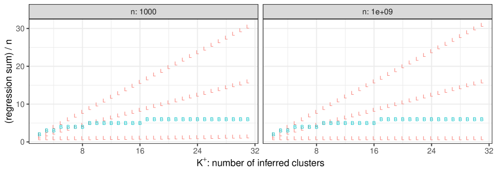
Figure 5: Scaled sum values of $(1+n^{-1}K^{+}(K^{+}-1)/2)$, $n^{-1}(K^{+}(n-K^{+}+1)+K^{+}(K^{+}-1)/2)$, $(K^{+}+1)/2$, and $(1+\lceil\log_{2}K^{+}\rceil)$ for various combinations of $n$ and $K^{+}$. The first three expressions are displayed as ‘L’ while the fourth expression is displayed as ‘B’.

Though these extreme scenarios provide useful computational cost bounds for a lopsided tree, seldom will they be even remotely close to how a leaf assignment $C_{\tau}$ will allocate observations. On the other hand, what exactly is a more “typical” allocation, and can we find an analytical representation for it or for a reasonable approximation of it? The answer to the former question (and hence also the latter question) depends on, among other things, the size of the data’s clusters and how well the mixture model infers these sizes. For simplicity, in the following exposition we will assume the mixture model infers $K^{+}$ leaf nodes each containing $n/K^{+}$ observations, in which case the sum for a lopsided tree becomes $n(K^{+}+1)/2$, which again is linear in $K^{+}$.

The final hurdle for this computational cost comparison between a lopsided tree and a balanced tree is that our three sum quantities for a lopsided tree, $n+K^{+}(K^{+}-1)/2$, $K^{+}(n-K^{+}+1)+K^{+}(K^{+}-1)/2$, and $n(K^{+}+1)/2$, are functions of $n$ and $K^{+}$ while the sum quantity for a balanced tree, $n\log_{2}K$, is a function of $n$ and $K$. How can we relate $K$ to $K^{+}$? We might optimistically assume the practitioner chose $K$ to be the smallest power of two greater than or equal to $K^{+}$, but we will “leave room for error” by instead assuming $K$ is the smallest power of two greater than or equal to $2K^{+}$, which implies $\log_{2}K=(1+\lceil\log_{2}K^{+}\rceil)$. Now all four sum quantities can be expressed as functions of $n$ and $K^{+}$ as shown in Figure 5. The (scaled) sum for a balanced tree grows logarithmically in $K^{+}$ whereas the (scaled) sum for the “typical” lopsided-tree scenario grows linearly, which explains why we find that training a balanced-tree mixture is usually faster than training its lopsided-tree counterpart.

9 GRIFOLS plots

10 Simulation study plots

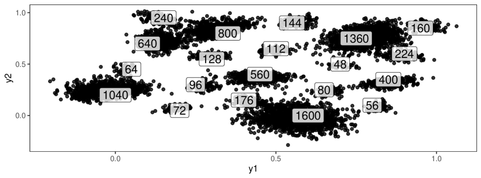
Figure 7: Data generated by 20 skew-normal distributions. The boxed numbers are the number of observations generated from each distribution.

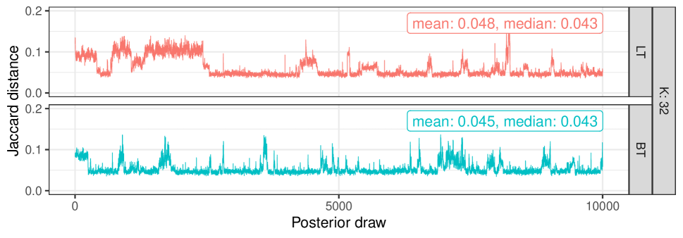
Figure 8: Jaccard distances at each posterior draw.

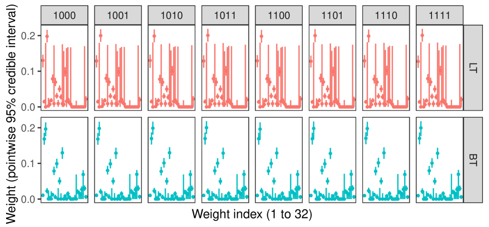
Figure 9: Inferred pointwise $95\%$ credible intervals for various covariate combinations.

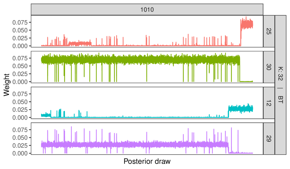
(a) Weights inferred by the balanced-tree mixture model for indices corresponding to wide credible intervals.

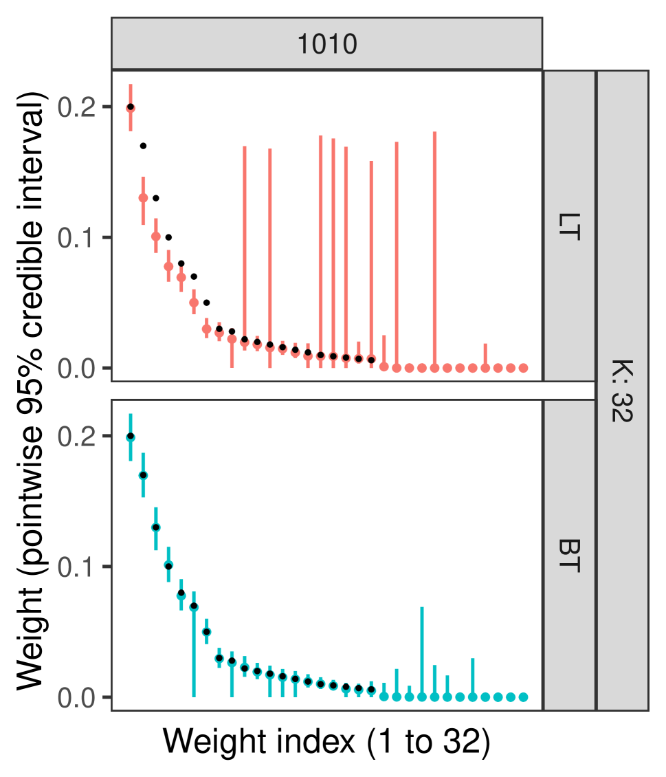
(b) Inferred pointwise $95\%$ credible intervals that are sorted by median weight. Points indicate the data’s true weight values.

(c) Inferred weights that are sorted before taking pointwise $95\%$ credible intervals. Points indicate the data’s true weight values.

Figure 10: Selected mixture-weight inference for $\mathbf{x}=1010$.

References

- Albert and Chib (1993) Albert, J. H. and S. Chib (1993). Bayesian analysis of binary and polychotomous response data. Journal of the American Statistical Association 88(422), 669–679.
- Bishop and Svensén (2002) Bishop, C. M. and M. Svensén (2002). Bayesian hierarchical mixtures of experts. In Proceedings of the Nineteenth conference on Uncertainty in Artificial Intelligence, pp. 57–64.
- Celeux et al. (2000) Celeux, G., M. Hurn, and C. P. Robert (2000). Computational and inferential difficulties with mixture posterior distributions. Journal of the American Statistical Association 95(451), 957–970.
- Cipolli and Hanson (2017) Cipolli, W. and T. Hanson (2017). Computationally tractable approximate and smoothed polya trees. Statistics and Computing 27(1), 39–51.
- Cron and West (2011) Cron, A. J. and M. West (2011). Efficient classification-based relabeling in mixture models. The American Statistician 65(1), 16–20.
- Fabius (1964) Fabius, J. (1964). Asymptotic behavior of bayes’ estimates. The Annals of Mathematical Statistics 34(4), 846–856.
- Ferguson (1973) Ferguson, T. S. (1973). A bayesian analysis of some nonparametric problems. The Annals of Statistics, 209–230.
- Foti and Williamson (2012) Foti, N. and S. Williamson (2012). Slice sampling normalized kernel-weighted completely random measure mixture models. Advances in Neural Information Processing Systems 25.
- Freedman (1963) Freedman, D. A. (1963). On the asymptotic behavior of bayes’ estimates in the discrete case. The Annals of Mathematical Statistics 34(4), 1386–1403.
- Frühwirth-Schnatter (2001) Frühwirth-Schnatter, S. (2001). Markov chain monte carlo estimation of classical and dynamic switching and mixture models. Journal of the American Statistical Association 96(453), 194–209.
- Ghosal and van der Vaart (2017) Ghosal, S. and A. van der Vaart (2017). Fundamentals of nonparametric Bayesian inference, Volume 44. Cambridge University Press.
- Gorsky et al. (2023) Gorsky, S., C. Chan, and L. Ma (2023). Coarsened mixtures of hierarchical skew normal kernels for flow and mass cytometry analyses. Bayesian Analysis 1(1), 1–25.
- Ishwaran and James (2001) Ishwaran, H. and L. F. James (2001). Gibbs sampling methods for stick-breaking priors. Journal of the American Statistical Association 96(453), 161–173.
- Ishwaran and James (2002) Ishwaran, H. and L. F. James (2002). Approximate dirichlet process computing in finite normal mixtures: smoothing and prior information. Journal of Computational and Graphical statistics 11(3), 508–532.
- Jaccard (1912) Jaccard, P. (1912). The distribution of the flora in the alpine zone. 1. New phytologist 11(2), 37–50.
- Jara and Hanson (2011) Jara, A. and T. E. Hanson (2011). A class of mixtures of dependent tail-free processes. Biometrika 98(3), 553–566.
- Jasra et al. (2005) Jasra, A., C. C. Holmes, and D. A. Stephens (2005). Markov chain monte carlo methods and the label switching problem in bayesian mixture modeling. Statistical Science 20(1), 50–67.
- Jordan and Jacobs (1994) Jordan, M. I. and R. A. Jacobs (1994). Hierarchical mixtures of experts and the em algorithm. Neural computation 6(2), 181–214.
- Maecker et al. (2012) Maecker, H. T., J. P. McCoy, and R. Nussenblatt (2012). Standardizing immunophenotyping for the human immunology project. Nat Rev Immunol 12(3), 191–200. Maecker, Holden T McCoy, J Philip Nussenblatt, Robert eng Z99 HL999999/Intramural NIH HHS/ ZIC HL005905-02/Intramural NIH HHS/ ZIC HL005905-03/Intramural NIH HHS/ ZIC HL005905-04/Intramural NIH HHS/ Review England 2012/02/22 Nat Rev Immunol. 2012 Feb 17;12(3):191-200. doi: 10.1038/nri3158.
- Mogilenko et al. (2022) Mogilenko, D. A., I. Shchukina, and M. N. Artyomov (2022). Immune ageing at single-cell resolution. Nat Rev Immunol 22(8), 484–498. Mogilenko, Denis A Shchukina, Irina Artyomov, Maxim N eng Research Support, Non-U.S. Gov’t Review England 2021/11/25 Nat Rev Immunol. 2022 Aug;22(8):484-498. doi: 10.1038/s41577-021-00646-4. Epub 2021 Nov 23.
- Papaspiliopoulos and Roberts (2008) Papaspiliopoulos, O. and G. O. Roberts (2008). Retrospective markov chain monte carlo methods for dirichlet process hierarchical models. Biometrika 95(1), 169–186.
- Papastamoulis (2016) Papastamoulis, P. (2016). label.switching: An r package for dealing with the label switching problem in mcmc outputs. Journal of Statistical Software, Code Snippets 69(1), 1–24.
- Peng et al. (1996) Peng, F., R. A. Jacobs, and M. A. Tanner (1996). Bayesian inference in mixtures-of-experts and hierarchical mixtures-of-experts models with an application to speech recognition. Journal of the American Statistical Association 91(435), 953–960.
- Polson et al. (2013) Polson, N. G., J. G. Scott, and J. Windle (2013). Bayesian inference for logistic models using pólya–gamma latent variables. Journal of the American statistical Association 108(504), 1339–1349.
- Puolamäki and Kaski (2009) Puolamäki, K. and S. Kaski (2009). Bayesian solutions to the label switching problem. In International Symposium on Intelligent Data Analysis, pp. 381–392. Springer.
- Redner and Walker (1984) Redner, R. A. and H. F. Walker (1984). Mixture densities, maximum likelihood and the em algorithm. SIAM review 26(2), 195–239.
- Ren et al. (2011) Ren, L., L. Du, L. Carin, and D. B. Dunson (2011). Logistic stick-breaking process. Journal of Machine Learning Research 12(1), 203–239.
- Rigon and Durante (2021) Rigon, T. and D. Durante (2021). Tractable bayesian density regression via logit stick-breaking priors. Journal of Statistical Planning and Inference 211, 131–142.
- Rodríguez and Dunson (2011) Rodríguez, A. and D. B. Dunson (2011). Nonparametric bayesian models through probit stick-breaking processes. Bayesian Analysis (Online) 6(1), 145–178.
- Rodríguez and Walker (2014) Rodríguez, C. E. and S. G. Walker (2014). Label switching in bayesian mixture models: Deterministic relabeling strategies. Journal of Computational and Graphical Statistics 23(1), 25–45.
- Sethuraman (1994) Sethuraman, J. (1994). A constructive definition of dirichlet priors. Statistica Sinica 4(2), 639–650.
- Stefanucci and Canale (2021) Stefanucci, M. and A. Canale (2021). Multiscale stick-breaking mixture models. Statistics and Computing 31(2), 1–13.
- Stephens (2000) Stephens, M. (2000). Dealing with label switching in mixture models. Journal of the Royal Statistical Society: Series B (Statistical Methodology) 62(4), 795–809.
- Wang and Roy (2018) Wang, X. and V. Roy (2018). Analysis of the pólya-gamma block gibbs sampler for bayesian logistic linear mixed models. Statistics & Probability Letters 137, 251–256.
- Yi et al. (2019) Yi, J. S., M. Rosa-Bray, J. Staats, P. Zakroysky, C. Chan, M. A. Russo, C. Dumbauld, S. White, T. Gierman, K. J. Weinhold, and J. T. Guptill (2019). Establishment of normative ranges of the healthy human immune system with comprehensive polychromatic flow cytometry profiling. PLoS One 14(12), e0225512.