Discontinuous normals in non-Euclidean geometries and two-dimensional gravity
Abstract
This paper builds two detailed examples of generalized normal in non-Euclidean spaces, i.e. the hyperbolic and elliptic geometries. In the hyperbolic plane we define a -sided hyperbolic polygon , which is the Euclidean closure of the hyperbolic plane , bounded by hyperbolic geodesic segments. The polygon is built by considering the unique geodesic that connects the vertices . The geodesics that link the vertices are Euclidean semicircles centred on the real axis. The vector normal to the geodesic linking two consecutive vertices is evaluated and turns out to be discontinuous. Within the framework of elliptic geometry, we solve the geodesic equation and construct a geodesic triangle. Also in this case, we obtain a discontinuous normal vector field. Last, the possible application to two-dimensional Euclidean quantum gravity is outlined.
1 Introduction
Suppose we want to measure the perimeter of a plane curve and we only have at our disposal a ruler, but not a whire that would match perfectly the boundary [1]. How are we going to evaluate the perimeter? One can indeed look for polygons whose sides are measurable with the help of the ruler, and one can “approximate” the shape of the curve by means of such polygons, asking ourselves the question by how much such polygons are close to the figure whose perimeter we want to evaluate. Within this framework, the very fruitful idea of Caccioppoli [2, 3] was to “measure” the distance between the polygon and the figure by means of the area of the difference set. In order to gain an idea of the perimeter, we have to take a sequence of polygons, such that the area of the difference set becomes smaller, and they will provide a sequence of approximate values of the perimeter. However, the area-type approximation of the figure can be obtained also by means of polygons having a perimeter unnecessarily large (for example, if we curl a polygon, we can achieve a very large perimeter). Thus, among all sequences of polygons which approximate a geometric figure, we must take, among the limits of their perimeters, the smallest value, i.e., the minimal limit of perimeters of the approximating polygons.
The development of geometric measure theory [2, 3, 4, 5, 6, 7, 8, 9, 10, 11, 12] led therefore to the discovery of many important concepts including, in particular, finite-perimeter sets with their reduced boundary (see definitions in A), two concepts that play an important role in modern mathematics. With hindsight, one can say that the divergence theorem does not hold on the topological boundary of a finite-perimeter set, but only on the reduced boundary, which is therefore the truly important concept of boundary. Let us here review some key aspects of this framework, which provide a motivation of our research.
If is a finite-perimeter set, the De Giorgi structure theorem ensures that its reduced boundary can be written in the form
| (1.1) |
where the are disjoint compact sets, and is a set having vanishing -dimensional Hausdorff measure. The sets are contained in -dimensional manifolds of class . If the point belongs to , one finds that the generalized normal to , denoted by , can be obtained by the equation
| (1.2) |
This means that the normal at is given by the normal existing at on the manifold (for this purpose, it is of crucial importance that the manifold should be of class ). Thus, the generalized normal is evaluated from the usual normal to a countable infinity of compact portions of smooth manifolds .
However, despite this profound result, the actual evaluation of the generalized normal may turn out to be impossible in some cases. In order to understand this feature, one can consider a dense sequence of points of . If the points are vectors with components which have rational coordinates
then within each ball centred at the point and having radius one can find infinitely many points, and the same is true outside such a ball. The desired set is in this case
| (1.3) |
and its volume can be majorized as follows:
| (1.4) |
where is the ball of unit radius. We have therefore defined a finite-volume set. Although no picture can be drawn, one can think of as consisting of infinitely many balls about the points of , which are dense in .
The topological boundary of coincides with the whole of minus . In fact, given a point of , one can find a sequence of points with rational coordinates, extracted from the sequence considered before. Such an extracted sequence tends to because the points with rational coordinates are dense. This means that is an accumulation point for . Thus belongs to the closure of . In turn, since is an open set (being formed by a countable union of open balls), the closure of is given by
| (1.5) |
and hence
| (1.6) |
Let us now prove that is a finite-perimeter set, despite the fact that its topological boundary has infinite volume. Indeed, by definition the perimeter is given by
| (1.7) |
where the integral over is a volume integral, and the defining conditions mean that is a vector field of norm never bigger than , of class on and having compact support on . By virtue of the definition (1.3), one can write the volume integral of the divergence of in the form
| (1.8) |
The union of a finite number of balls gives rise to an irregular set, because the balls do not have smooth intersections. Nevertheless, on such a set the divergence theorem holds, since such a set is piecewise smooth. One can therefore write, by virtue of the divergence theorem:
| (1.9) |
where is the normal to the topological boundary of the union of open balls, and is a surface measure. By virtue of (1.8) and (1.9), one finds the majorization ( being the measure of the surface given by the topological boundary of the union of open balls )
| (1.10) | |||||
where, on the first line, we have exploited the majorization of the norm of and the unit norm of , while on the second line we have exploited the property
| (1.11) |
This latter condition means that the topological boundary of the union of balls is in general smaller than the union of the various topological boundaries of such balls. Furthermore, we can re-express the majorization (1.10) as follows:
| (1.12) |
Indeed, if , one can find a constant for which
By virtue of (1.12), a real number exists such that
| (1.13) |
i.e. the set has a finite perimeter.
To sum up, the set defined in Eq. (1.3) is a finite-perimeter set of finite volume, while its topological boundary has infinite volume. Moreover, another consequence of De Giorgi’s structure theorem is that, if is a finite-perimeter set and if is a vector field of class , then
| (1.14) |
Thus, the divergence theorem holds for a finite-perimeter set, but it does not involve the whole of the topological boundary (because might contain parts that are too irregular to see the divergence of ). The divergence theorem involves therefore only the reduced boundary , which represents the truly useful part of the topological boundary . With hindsight, this is the ultimate meaning of De Giorgi’s structure theorem and of the concept of reduced boundary. The finite-perimeter sets are therefore the most general objects for which the divergence theorem still holds.
In the example we have investigated it is impossible to evaluate explicitly the generalized normal. Nevertheless, by virtue of De Giorgi’s structure theorem, we know some qualitative properties of great value: the reduced boundary is given by the countable union of pieces of manifolds of class , and the generalized normal is given by the normal to such manifolds. In such an example the reduced boundary is given by the countable union of pieces of smooth manifolds, and such pieces are represented by awkward-looking pieces of spherical surfaces. One can also prove, for this example, the inclusion property
| (1.15) |
i.e., the reduced boundary is a subset of the countable union of the topological boundaries of all open balls centred at and having radius .
It is therefore clear that every explicit construction of generalized normal is a challenging task which is nevertheless necessary if one wants to go beyond the purely qualitative properties. The following sections are devoted to two original examples, motivated by the desire to study geometric measure theory in non-Euclidean spaces. In particular, in Sec. 2 we deal with hyperbolic geometry, whereas the case of elliptic geometry is investigated in Sec. 3. The physical relevance of our framework is discussed in Sec. 4, where we consider possible applications to the action principle for two-dimensional Euclidean quantum gravity. In particular, we deal with the Euclidean two-dimensional Callan-Giddings-Harvey-Strominger (hereafter referred to as CGHS) dilaton gravity model [13, 14, 15] (see also Refs. [16, 17, 18, 19]). As we will show, a two-dimensional model makes it possible to overcome the issue regarding the definition of the normal vector in higher-dimensional theories such as general relativity (for recent reviews of general relativity and beyond, see, e.g., Refs. [20, 21, 22] and references therein). Last, concluding remarks are made in Sec. 5.
2 An example of generalized normal in the hyperbolic plane
The hyperbolic (or Lobachevsky) plane [23, 24, 25] is defined as the upper half-plane in the complex plane
| (2.1) |
endowed with the metric
| (2.2) |
Geodesics (or hyperbolic lines) in are defined in terms of Euclidean objects in , being represented either by (the intersection of with) Euclidean segments in perpendicular to the real axis or by (the intersection of with) Euclidean circles111Strictly speaking, we should distinguish between a circle and the associated circumference. in having Euclidean center on and Euclidean radius . Any two points in can be joined by a unique geodesic. Let be the piecewise differentiable path
| (2.3) |
defining a geodesic in . Bearing in mind (2.2), one finds that the geodesic (2.3) satisfies the following system of ordinary differential equations [26]:
| (2.4a) | |||||
| (2.4b) |
where and . When , the solution of (2.4b) is given by
| (2.5) |
representing a vertical line in . On the other hand, if is nonvanishing, the system (2.4b) leads to
| (2.6) |
which describes a Euclidean positive semicircle with Euclidean center at and Euclidean radius , since satisfies
| (2.7) |
It is not difficult to show that the Euclidean center and the Euclidean radius of the Euclidean circle through can be written as [24]
| (2.8a) | ||||
| (2.8b) | ||||
The hyperbolic length of a piecewise differentiable path
| (2.9) |
is given by
| (2.10) |
The hyperbolic distance between two points is defined by the formula
| (2.11) |
where the infimum is taken over all paths joining . Equation (2.11) defines a distance function on , since it is non-negative, symmetric, and satisfies the triangle inequality [23]. Moreover, it can be shown that for any [23]222When the points are such that , their hyperbolic distance reads as [23, 24]
| (2.12) |
The hyperbolic distance can also be written in terms of the Euclidean radius and the Euclidean center of the geodesic connecting as [24]
| (2.13) |
The group of all isometries of is isomorphic to the space , which is defined as follows:
This is equivalent to expressing as the quotient space because, if we change sign to all matrix entries, both and the determinant condition are preserved. Besides being a group, is also a topological space in which the fractional linear transformation can be identified with the point of . More precisely, as a topological space, can be identified with the following subset of :
If one defines
the map is therefore a homeomorphism, and we can write that
which is a more precise expression of the quotient space formula involving . Therefore is a topological group, and the fractional linear maps have a norm induced from given by
A hyperbolic -sided polygon is a closed set of (i.e., the Euclidean closure of ) bounded by hyperbolic geodesic segments. The vertices of , defined as the points of intersection of two line segments, can lie in , although no segment of can belong to [23].
An example which makes it possible for us to display an explicit expression for the dual normal can be constructed as follows. Let
| (2.14a) | ||||
| (2.14b) | ||||
| (2.14c) | ||||
| (2.14d) | ||||
| (2.14e) | ||||
| (2.14f) | ||||
denote the vertices of a hyperbolic -sided polygon . Such a polygon can be constructed by considering the unique geodesic connecting the following pairs of points: and , and , and , …, and , and eventually and . Since the points occurring in Eq. (2.14) have different real parts, all the aforementioned geodesics will be Euclidean positive semicircles having center on the real axis . The generic geodesic joining and will be defined by
| (2.15) |
where, from Eq. (2.4b), we have
| (2.16) | ||||
| (2.17) |
Therefore, we find that
| (2.18) | ||||
| (2.19) |
where
| (2.20) |
The unit normal vector to the geodesic (2.15) will be
| (2.21) |
with subjected to the conditions and .
We note that
| (2.22) |
which define an Euclidean degenerate circle. From the above equation jointly with formula (2.13), we find that
| (2.23) |
We note that the above result cannot be obtained by employing Eq. (2.12), since
| (2.24) |
meaning that does not belong to when (see B for further details). In this limit, Eq. (2.12) would lead to a meaningless result.
The geodesic connecting and
| (2.25) |
will have Euclidean center at and Euclidean radius , whereas for the geodesic through and
| (2.26) |
the Euclidean center lies at and the Euclidean radius is . From Eq. (2.8), we find
| (2.27) |
and
| (2.28) |
In the limit of large , we obtain
| (2.29) |
The unit normal vector to the geodesic (2.25) will be
| (2.30) |
satisfying the conditions and , whereas the unit normal vector to (2.26) is
| (2.31) |
where are such that the relations and are fulfilled.
The polygon having vertices (2.14) has thus a generalized normal represented by Eqs. (2.21), (2.30), and (2.31), i.e.,
| (2.32) |
It follows from the above equation that the -th segment of the polygon admits a normal vector which differs from the one of the -th segment. In other words, the generalized normal (2.32) defines a discontinuous vector field and, in the limit of large , assumes an infinite number of values. Furthermore, we note that in our example the reduced boundary of the polygon has a form which agrees with De Giorgi structure theorem (cf. Eq. (1.1)).
3 An example of generalized normal in elliptic geometry
In Euclidean geometry, given a line and a point which does not lie on this line, there exists one and only one line which passes through the given point and is parallel to the given line. On the other hand, in hyperbolic geometry, that we have considered in the previous section, infinitely many distinct parallel lines can be found. A third option, where no parallel lines exist, gives rise to elliptic geometry [27] and will be considered here. The most common model of elliptic geometry is represented by the surface of a sphere (however, it should be noted that in elliptic geometry two lines are usually assumed to intersect at a single point, while in spherical geometry two great circles intersect at two points, which is why spherical geometry is said to be a doubly elliptic geometry). Another relevant example of (two-dimensional) elliptic geometry is Klein’s conformal model of the elliptic plane [27].
In this section, we consider an example of two-dimensional elliptic geometry having squared line element [28]
| (3.1) |
The resulting connection coefficients read as
| (3.2) |
and hence the geodesic equations take the form
| (3.3a) | |||||
| (3.3b) |
where the prime denotes differentiation with respect to the affine parameter . If we eliminate the factor from the second equation and substitute it in the first, we get
| (3.4) |
which leads to
| (3.5) |
Then, from Eqs. (3.3b) and (3.5) we obtain the geodesic solutions
| (3.6) | ||||
| (3.7) |
where and are integration constants.
We note that the system (3.3b) is not affected if we interchange the role of and , i.e., it is invariant under the transformation
| (3.8) |
This means that
| (3.9) | ||||
| (3.10) |
is a solution of Eq. (3.3b), where are real-valued integration constants and
| (3.11) |
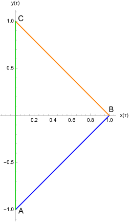
We can now set up a geodesic triangle by means of Eqs. (3.5)–(3.7). Let
| (3.12) |
be the vertices of (see Fig. 1).
Then, the side of connecting and is parametrized by
| (3.16) |
where
| (3.17) |
and the functions and can be obtained from Eqs. (3.6) and (3.7), respectively, by setting
| (3.18a) | ||||
| (3.18b) | ||||
| (3.18c) | ||||
The side , which links the vertices and , is defined by
| (3.22) |
The functions and can be read off from Eqs. (3.6) and (3.7), respectively, with
| (3.23a) | ||||
| (3.23b) | ||||
| (3.23c) | ||||
Last, can be obtained from
| (3.27) |
with
| (3.28) |
the functions and stemming Eqs. (3.6) and (3.7), respectively, when
| (3.29a) | ||||
| (3.29b) | ||||
| (3.29c) | ||||
It should be noted that the solution having can be regarded as a “limiting” case of Eqs. (3.5)–(3.7).
At this stage, we are ready to evaluate the normal vector field to the geodesic triangle . Given the curve , it is known that the equation of its normal to a generic point having coordinates is [29]
| (3.30) |
the prime denoting differentiation with respect to the variable. In our example, the geodesics can be equivalently described by means of (cf. Eq. (3.5))
| (3.31) |
which means that, recalling Eq. (3.18a), the equation of the side reads also as333It is clear that Eq. (3.32) can be obtained also from Eq. (3.16).
| (3.32) |
and hence by virtue of Eq. (3.30) the normal vector field to is defined by
| (3.33) |
where are the coordinates of a generic point belonging to . As a consequence of (3.23a) (or, equivalently, Eq. (3.22)), we have for the side
| (3.34) |
from which we derive the form of its normal vector field
| (3.35) |
being the coordinates of a point lying on . As pointed out before, the side cannot be obtained directly from (3.31). Indeed, its equation is
| (3.38) |
which means that is
| (3.39) |
4 Application to two-dimensional Euclidean quantum gravity
As far as we know, the kind of thinking used so far in our paper was lacking in the literature on fundamental interactions in physics. In recent times, much work in the mathematical literature has been devoted to the investigation of geometric measure theory in non-Euclidean spaces [30]. Within such a framework, the occurrence of discontinuous normal vector fields has to be considered [10], and our original explicit examples in Secs. 2 and 3 can be of interest.
On the other hand, the examples of Secs. 2 and 3 have a clear mathematical motivation, but they do not have an impact on theoretical physics. For this purpose, we are currently considering the case of Euclidean quantum gravity [31, 32, 33, 34, 35, 36, 37, 38, 39, 40]. Within this framework, a prescription for functional integration is necessary, and we propose to consider only finite-perimeter sets that match the assigned data on their reduced boundary. We arrive at this prescription upon bearing in mind that measurable sets belong to two families: either they have finite perimeter, or they do not. The restriction to finite-perimeter sets might be severe, but it leads to mathematical properties which are under control and hence merits a careful assessment.
A second choice is also in order, and it has to do with the dimension of such finite-perimeter sets. In higher dimensions a problem arises, i.e., how to define a vector that plays the role of normal. Even just for a straight line in three-dimensional Euclidean space, what is defined is the plane orthogonal to such a line, but there is no coordinate-independent way of selecting two linearly independent normal vector fields to the line. Thus, a four-dimensional analogue of our Secs. 2 and 3 is not conceivable, as far as we can see. We have therefore resorted to two-dimensional Euclidean quantum gravity, by focusing on the Euclidean two-dimensional CGHS dilaton gravity model [13, 14, 15] (see also e.g. Ref. [41] for a general framework pertaining to Euclidean dilaton gravity in two dimensions). This example will clarify the role of the discontinuous normal occurring in the divergence theorem (1.14).
The Euclidean CGHS action reads as
| (4.1) |
denoting the metric determinant, the Ricci scalar, the dilaton field, and a cosmological constant. Bearing in mind the recipes of Ref. [42] (see also Refs. [43, 44]), we can write the variations of the Lagrangian occurring in Eq. (4.1) as
| (4.2) |
where
| (4.3) |
are the metric and the dilaton field equations, respectively, and is referred to as the symplectic potential current density. By virtue of Eq. (4.1), we find
| (4.4a) | ||||
| (4.4b) | ||||
| (4.4c) | ||||
We aim at evaluating the integral
| (4.5) |
where is a two-dimensional region having finite perimeter. For this purpose, we find it more convenient to consider an off-shell calculation, i.e. for metric and dilaton field which do not obey the Euclidean field equations. In such a way, we may choose an example as close as possible to the ones developed in the theory of finite-perimeter sets in -dimensional Euclidean space [11], while avoiding the difficult task of solving the coupled partial differential equations for metric and dilaton.
4.1 Preparing the ground for evaluating the integral (4.5)
In order to prepare the ground for investigating the integral (4.5), let us consider the following example of two-dimensional finite-perimeter set [11], which provides a slight modification of the case discussed in Sec. 1 (which we recall is valid in with , see Eq. (1.12)). Consider in the set defined by
| (4.6) |
where, as before, denotes the Euclidean open ball centred at the point and having small positive radius , which is supposed to satisfy
| (4.7) |
such that
| (4.8) |
with
| (4.9) |
being the Euler -function. The perimeter of is
| (4.10) |
denoting the one-dimensional Hausdorff measure. Starting from Eq. (4.10), it can be shown [11] that for every , the set
| (4.11) |
has finite perimeter since, by virtue of Eq. (4.8),
| (4.12) |
Therefore, as ( being the volume of ), we have as and hence
| (4.13) |
which means that has finite perimeter. Furthermore, it is possible to prove that , which implies as a consequence [11].
We can now extend the previous example to a two-dimensional analytic Riemannian manifold . For this reason, let us consider the two-dimensional geodesic ball having small positive radius and centred at the point . The volume of can be written by means of the power series [45]
| (4.14) |
whereas the volume of reads as [45]
| (4.15) |
If the trace of the Ricci tensor is positive, then it follows from Eqs. (4.14) and (4.15) that, for sufficiently small ,
| (4.16) |
and
| (4.17) |
respectively.
At this stage, we have the necessary ingredients to generalize the previous example to the case when the manifold admits a positive trace of Ricci. Indeed, along the same lines as before, let
| (4.18) |
be a surface of constructed in terms of the geodesic balls whose radius is subject to the condition (4.8). Bearing in mind Eq. (4.17), we have
| (4.19) |
which makes it possible for us to prove that the set
| (4.20) |
has finite perimeter, since, similarly to Eq. (4.12),
| (4.21) |
Therefore, the set , which can be obtained from in the limit , has finite perimeter with
| (4.22) |
although .
5 Concluding remarks
By means of the methods presented in our paper, it is possible to evaluate the integral (4.5) over the finite-perimeter set , and we hope to have outlined the good potentialities of geometric measure theory for a fresh look at the unsolved problems of traditional formulations of Euclidean quantum gravity.
The next task wil be the rigorous proof of existence theorems of Euclidean functional integrals for gravity in two and higher dimensions, when restricted to finite-perimeter sets. If it were possible to accomplish this, the associated reduced boundary construction might open a new era in quantum gravity and quantum cosmology.
acknowledgments
E. B. is grateful to Nicola Fusco for invaluable discussions regarding many relevant topics of geometric measure theory. The authors thank Marco Abate for enlightening correspondence. This work is supported by the Austrian Science Fund (FWF) grant P32086. G. E. dedicates this research to Margherita.
Appendix A Finite-perimeter sets and their reduced boundary
On denoting by the characteristic function of a set (by definition, equals at points , and otherwise) and by the convolution product of two functions defined on :
| (A.1) |
De Giorgi defined [4, 5, 7] for all integer and for all the function
| (A.2) |
and, as a next step, the perimeter of the set
| (A.3) |
The perimeter defined in Eq. (A.3) is not always finite. A necessary and sufficient condition for to be finite is the existence of a set function of vector nature completely additive and bounded, defined for any set and denoted by , verifying the generalized Gauss-Green formula
| (A.4) |
If Eq. (A.4) holds, the function is said to be the distributional gradient of the characteristic function . A polygonal domain is every set that is the closure of an open set and whose topological boundary is contained in the union of a finite number of hyperplanes of . The sets approximated by polygonal domains having finite perimeter were introduced by Caccioppoli [2, 3] and coincide with the collection of all finite-perimeter sets [7]. This is why finite-perimeter sets are said to be Caccioppoli sets.
Is is a finite-perimeter set of , its reduced boundary is the collection of all points for which: (i) The integral of the norm of the gradient of the characteristic function, when taken over the ball (our ball is called open hypersphere by De Giorgi) centred at and of radius , is always positive, i.e.
| (A.5) |
(ii) The limit defining the normal vector exists, i.e.
| (A.6) |
(iii) The resulting normal vector has unit Euclidean norm.
Appendix B Calculation of the hyperbolic distance in the limit of large
In Sec. 2, we have evaluated the large- limit of the hyperbolic distance between the vertices and of the -sided hyperbolic polygon , defined by Eq. (2.14), by employing Eq. (2.13). The final result of this computation is displayed in Eq. (2.23). In this appendix, we show how the application of Eq. (2.12) for this calculation would have led to a misleading result.
Bearing in mind Eqs. (2.14e) and (2.14f), from Eq. (2.12) we obtain
| (B.1) |
and hence, in the limit of large , the above equation yields
| (B.2) |
Therefore, in Eq. (B.2) we recover a different result from the one given in Eq. (2.23). As pointed out before, this is due to the fact that the vertices and of the polygon do not belong, in the limit of large , to the hyperbolic plane , and hence Eq. (2.12) becomes meaningless under this hypothesis.
References
- [1] E. De Giorgi, Sviluppi dell’analisi funzionale nel novecento, in Renato Caccioppoli, la Napoli del suo tempo e la matematica del XX secolo, 63-79 (La Città del Sole, Napoli, 1987).
- [2] R. Caccioppoli, Elements of a general theory of -dimensional integration in a -dimensional space, Proceedings UMI Conference 2, 41-49 (1951).
- [3] R. Caccioppoli, Measure and integration on dimensionally oriented sets, Rend. Acc. Naz. Lincei Ser. 8 12, 3-11 (1952); ibid. 137-146 (1952).
- [4] E. De Giorgi, On a general theory of -dimensional measure in a -dimensional space, Ann. Mat. Pura Appl. (4) 36, 191-213 (1954).
- [5] E. De Giorgi, New theorems pertaining to -dimensional measures in -dimensional space, Ric. Mat. 4, 95-113 (1955).
- [6] H. Federer, Geometric Measure Theory (Springer, Berlin, 1969).
- [7] E. De Giorgi, F. Colombini, L. Piccinini, Frontiere Orientate di Misura Minima e Questioni Collegate (Editrice Tecnico Scientifica, Pisa, 1972).
- [8] E. Giusti, Minimal Surfaces and Functions of Bounded Variation (Birkhäuser, Boston, 1984).
- [9] L. Ambrosio, Corso Introduttivo alla Teoria Geometrica della Misura ed alle Superfici Minime (Edizioni della Normale, Pisa, 1996).
- [10] L. Ambrosio, N. Fusco, D. Pallara, Functions of Bounded Variation and Free Discontinuity Problems (Oxford University Press, Oxford, 2000).
- [11] F. Maggi, Finite Perimeter Sets and Geometric Variational Problems. An Introduction to Geometric Measure Theory (Cambridge University Press, Cambridge, 2012).
- [12] F. Bigolin, Teoria Geometrica della Misura (Aracne, Roma, 2012).
- [13] C. Callan, S. Giddings, J. Harvey, A. Strominger, Evanescent black holes, Phys. Rev. D 45, 1005 (1992).
- [14] J. Harvey, A. Strominger, Quantum Aspects of Black Holes, arXiv:hep-th/9209055.
- [15] A. Strominger, Les Houches lectures on black holes, Arxiv: hep-th/9501071
- [16] D. I. Kazakov, S. N. Solodukhin, On quantum deformation of the Schwarzschild solution, Nucl. Phys. B 429, 153 (1994).
- [17] A. Strominger, S. P. Trivedi, Information consumption by Reissner-Nordström black holes, Phys. Rev. D 48, 5778 (1993).
- [18] X. M. Deng, Geodesics and periodic orbits around quantum-corrected black holes, Physics of the Dark Universe 30, 100629 (2020).
- [19] B. Gao, X. M. Deng, Dynamics of charged test particles around quantum-corrected Schwarzschild black holes, Eur. Phys. J. C 81, 983 (2021).
- [20] L. Iorio, Editorial for the special issue 100 years of chronogeometrodynanics: The status of the Einstein’s theory of gravitation in its centennial year, Universe 1, 38 (2015).
- [21] I. Debono, G. F. Smoot, General relativity and cosmology: unsolved questions and future directions, Universe 2, 23 (2016).
- [22] R. G. Vishwakarma, Einstein and beyond: a critical perspective on general relativity, Universe 2, 16 (2016).
- [23] S. Katok, Fuchsian groups (The University of Chicago Press, Chicago and London, 1992).
- [24] J. Anderson, Hyperbolic geometry (Springer-Verlag, London, 2005).
- [25] T. Needham, Visual complex analysis (Clarendon Press, Oxford, 1999).
- [26] M. Nakahara, Geometry, Topology and Physics (IOP, Bristol, 2003).
- [27] H. S. M. Coxeter, Non-Euclidean geometry (The mathematical association of America, Washington, 1998).
- [28] D. E. Liebscher, The geometry of time (Wiley-VCH, New York, 2005).
- [29] G. Tortorici, Conferenze, esercizi e problemi sulle curve piane (Arti Grafiche A. Renna, Palermo, 1951).
- [30] https://cvgmt.sns.it
- [31] G. W. Gibbons, S. W. Hawking, Euclidean quantum gravity (World Scientific, Singapore, 1993).
- [32] G. Esposito, Quantum gravity, quantum cosmology and Lorentzian geometries (Springer, Berlin, 1994).
- [33] I. G. Avramidi, G. Esposito, A. Yu. Kamenshchik, Boundary operators in Euclidean quantum gravity, Class. Quantum Grav. 13, 2361 (1996).
- [34] G. Esposito, A.Yu. Kamenshchik, G. Pollifrone, Euclidean quantum gravity on manifolds with boundary (Kluwer, Dordrecht, 1997).
- [35] I. G. Avramidi, G. Esposito, Lack of strong ellipticity in Euclidean quantum gravity, Class. Quantum Grav. 15, 1141 (1998).
- [36] G. Esposito, Non-local boundary conditions in Euclidean quantum gravity, Class. Quantum Grav. 16, 1113 (1999).
- [37] G. Esposito, G. Fucci, A. Yu. Kamenshchik, K. Kirsten, Spectral asymptotics of Euclidean quantum gravity with diff-invariant boundary conditions, Class. Quantum Grav. 22, 957 (2005).
- [38] G. Esposito, G. Fucci, A. Yu. Kamenshchik, K. Kirsten, A non-singular one-loop wave function of the universe from a new eigenvalue asymptotics in quantum gravity, JHEP 09, 063 (2005).
- [39] E. Battista, G. Esposito, What is a reduced boundary in general relativity?, Int. J. Mod. Phys. D 30, 2150050 (2021).
- [40] E. Witten, A note on boundary conditions in Euclidean gravity, Rev. Math. Phys. 33, 2140004 (2021).
- [41] L. Bergamin, D. Grumiller, W. Kummer, D. Vassilevich, Classical and quantum integrability of 2D dilaton gravities in euclidean space, Class. Quant. Grav. 22, 1361 (2005).
- [42] J.Lee, R. Wald, Local symmetries and constraints, J. Math. Phys. 31, 725 (1990).
- [43] T. Jacobson, G. Kang, R. Myers, On black hole entropy, Phys. Rev. D 49, 6587 (1994).
- [44] R. Myers, Black hole entropy in two dimensions, Phys. Rev. D 50, 6412 (1994).
- [45] A. Gray, The volume of a small geodesic ball of a Riemannian manifold, Michigan Math. J. 20, 329-344 (1973).