A perturbative approximation to DFT/MRCI: DFT/MRCI(2)

Abstract

We introduce a perturbative approximation to the combined density functional theory and multireference configuration interaction (DFT/MRCI) method. The method, termed DFT/MRCI(2), results from the application of quasi-degenerate perturbation theory and the Epstein-Nesbet partitioning of the DFT/MRCI Hamiltonian matrix. This results in the replacement of the diagonalization of the large DFT/MRCI Hamiltonian with that of a small effective Hamiltonian, and affords orders of magnitude savings in terms of computational cost. Moreover, the DFT/MRCI(2) approximation is found to be of excellent accuracy, furnishing excitation energies with a root mean squared deviation from the DFT/MRCI values of less than 0.03 eV for an extensive test set of organic molecules.

I Introduction

First formulated by Grimme and WaletzkeGrimme and Waletzke (1999), the combined density functional theory and multireference configuration interaction (DFT/MRCI) method fills a unique niche in the landscape of excited-state electronic structure theory. In particular, DFT/MRCI possesses the following desirable characteristics: (i) the possibility of a “black box” implementation; (ii) high accuracy in vertical excitation energies; (iii) low computational cost, rendering it applicable to large molecules, and; (iv) an ability to describe a large range of electronic states, including those of multireference, Rydberg, doubly-excited and charge transfer character.

Originally conceived as a method for the description of singlet and triplet states of organic moleculesGrimme and Waletzke (1999), recent years have seen the development of DFT/MRCI Hamiltonians that are multiplicity agnosticLyskov et al. (2016); Heil and Marian (2017); Marian et al. (2019), and tailored to the description of transition metal complexesHeil et al. (2018). It has also been recently demonstrated that DFT/MRCI may be successfully applied to the calculation of core-excited states via the application of the core-valence separation approximationSeidu et al. (2019). In addition to excitation energies, a plethora of properties may be reliably computed using DFT/MRCI, including spin-orbit couplingKleinschmidt et al. (2006); Kleinschmidt and Marian (2005), diabatic potentials and couplingsNeville et al. (2020), and numerical derivative couplingsBracker et al. (2021).

Recently, a new DFT/MRCI pruning algorithm was introducedNeville and Schuurman (2021a), in which deadwood configurations are removed based on an estimate of their contribution to the wave functions of interest made using Rayleigh Schrödinger perturbation theory (RSPT) in conjunction with the Epstein-Nesbet Hamiltonian partitioningEpstein (1926); Nesbet and Hartree (1955). The resulting method, termed p-DFT/MRCI, was shown to retain the accuracy of the original DFT/MRCI method, but with configuration spaces reduced in size by up to two orders of magnitude. This result suggests that perturbative approximations based on the Epstein-Nesbet Hamiltonian partitioning are well suited to pairing with the DFT/MRCI. We here explore taking this approach to its logical conclusion: the complete replacement of the expensive diagonalization of the DFT/MRCI Hamiltonian matrix with a perturbative approximation of its eigenpairs.

The approach pursued here is to use quasi-degenerate perturbation theory (QDPT) to replace the DFT/MRCI Hamiltonian with a small effective Hamiltonian that may be fully diagonalized to yield approximations to the DFT/MRCI states and energies. In particular, we explore the combination of generalized van Vleck perturbation theory (GVVPT)Kirtman (1981); Hirschfelder (1978); Certain and Hirschfelder (1970); Certain et al. (1970) with the Epstein-Nesbet Hamiltonian partitioning. The resulting method, which we term DFT/MRCI(2), is shown to yield excellent approximations to the DFT/MRCI excitation energies, exhibiting a root mean square deviation of the order of $10^{-2}$ eV for a comprehensive test set. Moreover, the cost of building and diagonalizing the DFT/MRCI(2) effective Hamiltonian matrix is dramatically reduced in comparison to the iterative diagonalization of the full DFT/MRCI Hamiltonian and affords computational savings expected to reach three orders of magnitude for large molecules.

The rest of the paper is structured as follows. In Section II, we provide a brief overview of the DFT/MRCI method. In Section III, we give the details of the DFT/MRCI(2) approximation and working equations. A set of benchmarking and example calculations are presented in Section IV, followed by concluding remarks and outlooks in Section V.

II DFT/MRCI

II.1 The DFT/MRCI wave function and Hamiltonian matrix

In common with all MRCI approaches, the DFT/MRCI wave function ansatz may be written as

$$|\Psi_{I}\rangle=\sum_{\Omega\in\mathcal{R}}C_{\Omega}^{(I)}|\Omega\rangle+\sum_{\Omega\in\mathcal{F}}C_{\Omega}^{(I)}|\Omega\rangle,$$ (1)

where, $|\Omega\rangle$ denote spin-adapted configuration state functions (CSFs). The total CSF space is partitioned into a reference space $\mathcal{R}$ and the first-order interacting space (FOIS) $\mathcal{F}$, obtained by the application of one- and two-electron excitation operators to $\mathcal{R}$. Here, the comparatively small reference space is chosen to yield a qualitatively correct description of the states $|\Psi_{I}\rangle$ of interest, capturing the pertinent static electron correlation. The FOIS CSFs account for the remaining dynamic electron correlation. The FOIS, in contrast to the reference space, is generally large in size, and the diagonalization of the electronic Hamiltonian projected onto the space spanned by $\mathcal{R}\cup\mathcal{F}$ quickly becomes an extremely demanding computational task.

The DFT/MRCI method seeks to circumvent this issue through the introduction of DFT-specific on-diagonal Hamiltonian matrix corrections to recover the majority of the dynamic correlation that would otherwise be captured by the interaction of the reference space and FOIS CSFs. Let each CSF $|\Omega\rangle$ be specified by a spatial orbital occupation w and a spin-coupling pattern $\omega$: $|\Omega\rangle=|\textbf{w}\omega\rangle$. Then, the DFT-specific corrections take the form of the following modifications of the on-diagonal Hamiltonian matrix elementsGrimme and Waletzke (1999):

$$\left\langle\textbf{w}\omega\middle|\hat{H}^{DFT}-E_{DFT}\middle|\textbf{w}\omega\right\rangle =\left\langle\textbf{w}\omega\middle|\hat{H}-E_{SCF}\middle|\textbf{w}\omega\right\rangle$$ (2)

$$+\sum_{p}\Delta\text{w}_{p}\left(\epsilon_{p}^{KS}-F_{pp}\right)$$

$$+\Delta E_{x}+\Delta E_{c}.$$

Here, $\Delta\text{w}_{p}=\text{w}_{p}-\overline{\text{w}}_{p}$ denotes the difference of the occupation of the $p$th spatial orbital relative to a base, or anchor, occupation $\overline{\textbf{w}}$, chosen as the Hartree-Fock (HF) occupation. $\epsilon_{p}^{KS}$ and $F_{pp}$ denote, respectively, the Kohn-Sham (KS) orbital energies and on-diagonal elements of the Fock operator in the KS orbital basis. Finally, $\Delta E_{x}$ and $\Delta E_{c}$ are Coulomb and exchange corrections, the exact form of which varies with the different DFT/MRCI parameterizationsGrimme and Waletzke (1999); Lyskov et al. (2016); Heil and Marian (2017); Heil et al. (2018).

Underlying these semi-empirical corrections is the recognition that differences between diagonal Fock matrix elements contribute, in a zeroth-order manner, to the on-diagonal Hamiltonian matrix elements (see, e.g., the work of Segal, Wetmore and WolfWetmore and Segal (1975); Segal et al. (1978)). The differences between KS orbital energies are typically closer to ground-to-excited-state excitation energies than the corresponding differences in Fock matrix elements. Building these into the on-diagonal Hamiltonian matrix elements, and appropriately down-scaling the Coulomb and exchange terms that appear alongside, one may effectively incorporate a large amount of dynamic electron correlation that would otherwise be accounted for by the coupling of the reference and FOIS CSFs. To avoid a double counting of dynamic correlation, the off-diagonal Hamiltonian matrix elements must be appropriately adjusted. This is achieved through the introduction of a damping of the off-diagonal elements that is dependent on the energetic separation of the bra and ket CSFs:

$$\left\langle\textbf{w}\omega\middle|\hat{H}^{DFT}-E_{DFT}\middle|\textbf{w}^{\prime}\omega^{\prime}\right\rangle =\left\langle\Omega\middle|\hat{H}-E_{SCF}\middle|\Omega^{\prime}\right\rangle$$ (3)

$$\times D(\Delta E_{\Omega\Omega^{\prime}}),$$

where

$$\Delta E_{\Omega\Omega^{\prime}}=\frac{1}{n_{\omega}}\sum_{\omega}^{n_{\omega}}H_{\Omega,\Omega}^{DFT}-\frac{1}{n_{\omega^{\prime}}}\sum_{\omega^{\prime}}^{n_{\omega^{\prime}}}H_{\Omega^{\prime},\Omega^{\prime}}^{DFT}$$ (4)

denotes the spin coupling-averaged difference between the on-diagonal matrix elements corresponding to the spatial occupations w and $\textbf{w}^{\prime}$, which generate $n_{\omega}$ and $n_{\omega^{\prime}}$ CSFs, respectively. The damping function $D(\Delta E)$ is chosen to decay rapidly with increasing $\Delta E$: in practice chosen as either an exponentialGrimme and Waletzke (1999); Heil et al. (2018) or inverse arctangentLyskov et al. (2016); Heil and Marian (2017) function. In this way, the coupling of energetically distant reference and FOIS CSFs is damped to near-zero, thereby avoiding to a large extent a double counting of dynamic correlation effects.

This decoupling of a large part of the FOIS from the reference space means that most of the FOIS CSFs are no longer required. These are identified a priori using a simple orbital energy-based selection criterionGrimme and Waletzke (1999), which proceeds as follows. For each FOIS configuration w, the quantity

$$d_{\textbf{w}}=\sum_{p}\Delta\text{w}_{p}\epsilon_{p}^{KS}-\delta E_{sel}$$ (5)

is computed, where $\delta E_{sel}$ is a parameter with a value conventionally chosen as either 1.0 or 0.8 E${}_{\text{h}}$. If $d_{\textbf{w}}$ is less than the highest reference space eigenvalue of interest, then all the CSFs generated from the configuration w are selected for inclusion, else they are discarded. This configuration selection step results in a massive reduction of the size of the CSF basis, typically by many orders of magnitude, and results in huge speedups relative to an ab initio MRCI calculation.

II.2 Reference space selection and refinement

One appealing property of DFT/MRCI is that, being an individually selecting CI method, arbitrary reference spaces may be used, imbuing the method with great flexibility. Moreover, a DFT/MRCI calculation is typically performed in the following iterative fashion. First, a standard DFT/MRCI calculation is performed using an initial, guess reference space $\mathcal{R}_{0}$. The resulting eigenvectors are then analyzed and a new, improved reference space $\mathcal{R}_{1}$ is constructed which contains all the configurations that generate one or more of the CSFs contributing significantly to the states of interest. Another DFT/MRCI calculation is then performed using the refined reference space, and this procedure is repeated until the reference space is converged.

This reference space refinement procedure may be automated, and all that is left is to specify the initial reference space $\mathcal{R}_{0}$. Recently, a fully automated algorithm for the construction of $\mathcal{R}_{0}$ was introducedNeville and Schuurman (2021a), in which a preliminary approximate combined DFT and CI singles (DFT/CIS)Grimme (1996) calculation is used to identify a subset of orbitals from which compact, but qualitatively correct, restricted active space CI (RASCI)Olsen et al. (1988) reference spaces may be constructed. The result is a completely black box calculation, requiring only the number of states to be specified by the user. Moreover, the ability to automatically and reliably construct initial reference spaces that yield good zeroth-order descriptions of the states of interest is of utmost importance if perturbative approximations are to be introduced, as is the focus this paper.

III DFT/MRCI(2)

To arrive at a robust and easily implemented perturbative approximation to the DFT/MRCI method, we consider the application of the Epstein-Nesbet Hamiltonian partitioningEpstein (1926); Nesbet and Hartree (1955) in conjunction with QDPTBRANDOW (1967); Löwdin and Goscinski (1971); Lindgren (1974); Klein (1974); Kvasnička (1977); Hose and Kaldor (1979); Shavitt and Redmon (1980). In particular, we consider use of the GVVPT variant of QDPTKirtman (1981). This combination, when applied to the DFT/MRCI Hamiltonian, results in the DFT/MRCI(2) approximation.

III.1 Generalized van Vleck perturbation theory

To keep the present discussion self-contained, we will here give a brief overview of the generalized van Vleck variant of QDPT, focusing on the aspects pertinent to the development of the DFT/MRCI(2) method. The starting point is the partitioning of the total Hamiltonian $\hat{H}$ as the sum of a zeroth-order operator $\hat{H}_{0}$ and a perturbation $\hat{V}$:

$$\hat{H}=\hat{H}_{0}+\hat{V}.$$ (6)

Let $|\Psi_{k}^{(0)}\rangle$ denote the eigenfunctions of the zeroth-order Hamiltonian $\hat{H}_{0}$, with associated eigenvalues $E_{k}^{(0)}$,

$$\hat{H}_{0}|\Psi_{k}^{(0)}\rangle=E_{k}^{(0)}|\Psi_{k}^{(0)}\rangle.$$ (7)

In the GVVPT scheme, the set $\{|\Psi_{k}^{(0)}\rangle\}$ is subdivided into a “model space” $\mathcal{M}=\{|\phi_{i}\rangle\}$ and an “external space” $\mathcal{E}=\{|\chi_{a}\rangle\}$. The model space $\mathcal{M}$ is to be equated with with the zeroth-order states $|\Psi_{k}^{(0)}\rangle$ for which perturbative corrections are sought, and the external space $\mathcal{E}$ with their orthogonal complement.

In common with all QDPT variants, in GVVPT a similarity transformation $\boldsymbol{U}$ is sought that block diagonalizes the Hamiltonian such that the model and external spaces are decoupled:

$$\boldsymbol{U}^{-1}\boldsymbol{H}\boldsymbol{U}=\boldsymbol{\mathcal{H}}=\begin{bmatrix}\boldsymbol{\mathcal{H}}_{\mathcal{M}\mathcal{M}}&\boldsymbol{0}\\ \boldsymbol{0}&\boldsymbol{\mathcal{H}}_{\mathcal{E}\mathcal{E}}\end{bmatrix}.$$ (8)

Diagonalization of the model space block, $\boldsymbol{\mathcal{H}}_{\mathcal{M}\mathcal{M}}$, of the effective Hamiltonian $\boldsymbol{\mathcal{H}}$ then yields the energies of the states of interest.

Let $\{|\tilde{\phi}_{i}\rangle\}$ and $\{|\tilde{\chi}_{a}\rangle\}$ denote the sets of perturbed model and external states, respectively, that result from the block diagonalization transformation $\boldsymbol{U}$. To proceed, these are expanded in a perturbation series,

$$|\tilde{\phi}_{i}\rangle=|\phi_{i}\rangle+|\phi_{i}^{(1)}\rangle+|\phi_{i}^{(2)}\rangle+\cdots,$$ (9)

$$|\tilde{\chi}_{a}\rangle=|\chi_{a}\rangle+|\chi_{a}^{(1)}\rangle+|\chi_{a}^{(2)}\rangle+\cdots.$$ (10)

In the GVVPT method, perturbative approximations for the model space block, $\boldsymbol{\mathcal{H}}_{\mathcal{M}\mathcal{M}}$ of the effective Hamiltonian and the perturbed model states $\{|\tilde{\phi}_{i}\rangle\}$ are determined by the enforcement of the following two conditions: (i) that the effective Hamiltonian is block diagonal in the perturbed basis, and; (ii) that the perturbed basis is orthogonal within the model space and between the model and external spaces. This results in the following form of the second-order effective Hamiltonian within the model spaceKirtman (1981):

$$\mathcal{H}_{ij}^{[2]} =\langle\phi_{i}|\hat{H}_{0}|\phi_{j}\rangle+\langle\phi_{i}|\hat{V}|\phi_{j}\rangle$$ (11)

$$+\frac{1}{2}\left[\langle\phi_{i}|\hat{V}\hat{R}_{j}\hat{V}|\phi_{j}\rangle+\langle\phi_{i}|\hat{V}\hat{R}_{i}\hat{V}|\phi_{j}\rangle\right],$$

where the resolvant operator $\hat{R}_{i}$ is defined as

$$\hat{R}_{i}=\sum_{a}|\chi_{a}\rangle\left(E_{i}^{(0)}-E_{a}^{(0)}\right)^{-1}\langle\chi_{a}|$$ (12)

The first-order perturbed model states are given by

$$|\tilde{\phi}_{i}^{[1]}\rangle=|\phi_{i}\rangle+\hat{R}_{i}\hat{V}|\phi_{i}\rangle.$$ (13)

Diagonalization of the model space block of $\boldsymbol{\mathcal{H}}^{[2]}$ yields the second-order GVVPT (GVVPT2) approximations, $E_{I}^{[2]}$, of the energies of the states of interest,

$$\boldsymbol{E}^{[2]}=\text{diag}\left(E_{1}^{[2]},E_{2}^{[2]},\dots,E_{m}^{[2]}\right)=\boldsymbol{X}^{T}\boldsymbol{\mathcal{H}}_{\mathcal{M}\mathcal{M}}^{[2]}\boldsymbol{X}$$ (14)

Finally, first-order corrected wave functions $|\Psi_{I}^{[1]}\rangle$ may be computed using the eigenvectors $\boldsymbol{X}$ and first-order perturbed model states $|\tilde{\phi}_{i}^{[1]}\rangle$:

$$|\Psi_{I}\rangle\approx|\Psi_{I}^{[1]}\rangle=\sum_{i}X_{iI}|\tilde{\phi}_{i}^{[1]}\rangle.$$ (15)

III.2 Epstein-Nesbet Hamiltonian partitioning

To arrive at working equations, the form of the Hamiltonian partitioning (i.e., $\hat{H}_{0}$ and $\hat{V}$) needs to be specified. We adopt the Epstein-Nesbet partitioning, in which the total set of CSFs $\{\Omega\}$ is partitioned into two subspaces, termed the $\mathcal{P}$ and $\mathcal{Q}$ spaces. The zeroth-order Hamiltonian is taken to be block diagonal between the $\mathcal{P}$ and $\mathcal{Q}$ spaces and diagonal within the $\mathcal{Q}$ space:

$$\hat{H}_{0}=\sum_{\Omega,\Omega^{\prime}\in\mathcal{P}}|\Omega\rangle\langle\Omega|\hat{H}|\Omega^{\prime}\rangle\langle\Omega^{\prime}|+\sum_{\Omega\in\mathcal{Q}}|\Omega\rangle\langle\Omega|\hat{H}|\Omega\rangle\langle\Omega|.$$ (16)

The perturbation accounts for the missing coupling between the $\mathcal{P}$ and $\mathcal{Q}$ spaces and that within the $\mathcal{Q}$ space:

$$\hat{V} =\left\{\sum_{\begin{subarray}{c}\Omega\in\mathcal{P}\\ \Omega^{\prime}\in\mathcal{Q}\end{subarray}}|\Omega\rangle\langle\Omega|\hat{H}|\Omega^{\prime}\rangle\langle\Omega^{\prime}|+h.c.\right\}$$ (17)

$$+\sum_{\begin{subarray}{c}\Omega,\Omega^{\prime}\in\mathcal{Q}\\ \Omega\neq\Omega^{\prime}\end{subarray}}|\Omega\rangle\langle\Omega|\hat{H}|\Omega^{\prime}\rangle\langle\Omega^{\prime}|$$

Within the context of a DFT/MRCI calculation, the natural choice is to identify the $\mathcal{P}$ space with the reference space ($\mathcal{P}=\mathcal{R}$) and the $\mathcal{Q}$ with the FOIS CSFs that have survived the configuration selection criterion ($\mathcal{Q}\subset\mathcal{F}$), and this shall be assumed in the following.

III.3 DFT/MRCI(2) working equations

We now consider the combination of GVVPT2 with the Epstein-Nesbet Hamiltonian partitioning and, in particular, the application of these to the DFT/MRCI Hamiltonian matrix. In order to calculate the energies of the $N$ states, we choose that the model space to be spanned by the $N$ lowest-lying reference space eigenfunctions of interest, $|\Psi_{I}^{(0)}\rangle$, with corresponding energies $E_{I}^{(0)}$, plus a small set of additional ‘buffer’ states $\{|\Psi_{I}^{(0)}\rangle|I=N+1,\dots,N+N_{buf}\}$. Substitution of Equations 16 and 17 into Equation 11, and replacing the ab initio Hamiltonian $\hat{H}$ with the DFT/MRCI Hamiltonian $\hat{H}^{DFT}$, we obtain the following expression for the DFT/MRCI(2) effective Hamiltonian:

$$\left[\boldsymbol{\mathcal{H}}_{DFT}^{[2]}\right]_{IJ}=\delta_{IJ}E_{I}^{(0)}+\frac{1}{2}\sum_{i=I,J}\sum_{\Omega\in\mathcal{Q}}\frac{B_{\Omega I}B_{\Omega J}}{E_{i}^{(0)}-E_{\Omega}^{(0)}},$$ (18)

where

$$B_{\Omega I}=\langle\Omega|\hat{H}^{DFT}|\Psi_{I}^{(0)}\rangle,$$ (19)

$$E_{\Omega}^{(0)}=\langle\Omega|\hat{H}^{DFT}|\Omega\rangle,$$ (20)

and real CSFs have been assumed.

Similarly, the DFT/MRCI(2) first-order corrected eigenfunctions are given by

$$|\Psi_{I}^{[1]}\rangle=\sum_{J}X_{JI}\left[|\Psi_{J}^{(0)}\rangle+\sum_{\Omega\in\mathcal{Q}}\left(\frac{B_{\Omega J}}{E_{J}^{(0)}-E_{\Omega}^{(0)}}\right)|\Omega\rangle\right],$$ (21)

where $\boldsymbol{X}$ is the matrix of eigenvectors of $\boldsymbol{\mathcal{H}}_{DFT}^{[2]}$.

We note that all the matrix elements required to evaluate Equations 18 and 21 are also needed in the calculation of the DFT/MRCI Hamiltonian matrix. Thus, it is a somewhat trivial task to modify an existing DFT/MRCI code to compute the DFT/MRCI(2) effective Hamiltonian and first-order corrected eigenfunctions. We emphasize here that the calculation of these quantities requires significantly less computational effort than the iterative diagonalization of the DFT/MRCI Hamiltonian matrix.

III.4 Dynamical reference space refinement

The refinement of the DFT/MRCI(2) reference space proceeds in an analogous manner to that of a DFT/MRCI calculation except that the DFT/MRCI wave functions are replaced with their first-order corrected approximations $|\Psi_{I}^{[1]}\rangle$. The automated, DFT/CIS-based initial reference space generation algorithm described in Section II.2 is used in our implementation of DFT/MRCI(2). This generally results in initial reference spaces with excellent support of the states of interest. However, in practice, we have encountered a small number of situations in which the thus generated initial reference space is only of moderate quality, as measured by the norm of the projection of the first-order corrected eigenfunctions onto the $\mathcal{Q}$ space,

$$Q_{I}=\left|\left|\sum_{\Omega\in\mathcal{Q}}|\Omega\rangle\langle\Omega|\Psi_{I}^{[1]}\rangle\right|\right|.$$ (22)

When $Q_{I}$ is large, the first-order corrected eigenfunctions may only be qualitatively correct. In such a case, a more relaxed configuration selection threshold may be beneficial in the reference space refinement step. We have thus implemented the following state-specific, dynamical configuration selection threshold:

$$\epsilon(Q_{I})=\max\left(\epsilon_{min},\frac{\epsilon_{max}}{\cosh^{2}\left(\mu Q_{I}\right)}\right).$$ (23)

If the CSF $|\Omega\rangle$ has a coefficient for state $I$ with an absolute value greater than $\epsilon(Q_{I})$, then the corresponding configuration is chosen for inclusion in the refined reference space. In this work, empirical parameter values of $\epsilon_{min}=0.015$, $\epsilon_{max}=0.055$, and $\mu=3.3$ have been used. For reference, the dynamic selection threshold $\epsilon(Q_{I})$ is shown plotted in Figure 1 for these values.

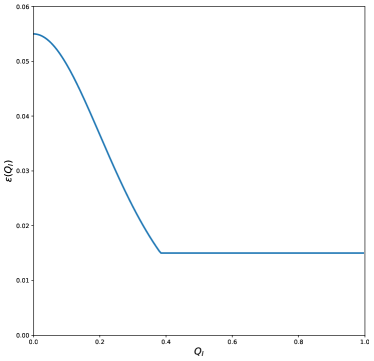
Figure 1: Dynamic configuration selection threshold function $\epsilon(Q_{I})$ used in all DFT/MRCI(2) calculations for parameter values $\epsilon_{min}=0.015$, $\epsilon_{max}=0.055$, and $\mu=3.3$. See Equation 23 for the definition of this function.

III.5 Intruder states

In practice, there may exist $\mathcal{Q}$ space CSFs $|\Omega\rangle$ that are near degenerate with one of the reference space states $|\Psi_{I}^{(0)}\rangle$ of interest. This is most likely to occur in the first iteration of the reference space refinement in which a guess/unrefined reference space $\mathcal{R}_{0}$ is employed. For a given pair of states $I$ and $J$, we will obtain effective Hamiltonian matrix elements $\left|\left[\boldsymbol{\mathcal{H}}_{DFT}^{[2]}\right]_{IJ}\right|\rightarrow\infty$ if there exists a $\mathcal{Q}$ space CSF $|\Omega\rangle$ satisfying

$$\left|E_{i}^{(0)}-E_{\Omega}^{(0)}\right|\rightarrow 0,\hskip 14.22636pti=I\text{ or }i=J.$$ (24)

Such a CSF is referred to as an “intruder state”.

To ameliorate this problem, we adopt the intruder state avoidance (ISA) technique of Witek et al.Witek et al. (2002). Here, the energy denominators appearing in Equations 18 and 21 are subjected to the replacement

$$\left(E_{I}^{(0)}-E_{\Omega}^{(0)}\right)^{-1}\rightarrow\left(E_{I}^{(0)}-E_{\Omega}^{(0)}+\Delta_{\Omega I}\right)^{-1},$$ (25)

where

$$\Delta_{\Omega I}=\frac{b}{E_{I}^{(0)}-E_{\Omega}^{(0)}},$$ (26)

with $b\in\mathbb{R}$ being a free parameter. The shift $\Delta_{\Omega I}$ satisfies

$$\left|\Delta_{\Omega I}\right|\rightarrow\infty\hskip 14.22636pt\text{as}\hskip 14.22636pt\left|E_{I}^{(0)}-E_{\Omega}^{(0)}\right|\rightarrow 0.$$ (27)

Thus, the contributions from any intruder states are damped out, and the appearance of (near) singularities in the DFT/MRCI(2) working equations is avoided.

Care must be taken in the application of the ISA technique within the framework of a DFT/MRCI(2) calculation due to the iterative reference space refinement procedure. Here, the initial/guess reference space being updated to include all configurations contributing significantly to the DFT/MRCI(2) first-order corrected eigenstates $|\Psi_{I}^{[1]}\rangle$. However, the coefficients for any intruder states will be damped to near zero when using the ISA scheme, resulting in their exclusion from the refined reference space. To remedy this, the terms

$$C_{\Omega I}=B_{\Omega I}\left(E_{I}^{(0)}-E_{\Omega}^{(0)}\right)^{-1}$$ (28)

and

$$\overline{C}_{\Omega I}=B_{\Omega I}\left(E_{I}^{(0)}-E_{\Omega}^{(0)}+\Delta_{\Omega I}\right)^{-1}$$ (29)

are computed during the course of the calculation of the effective Hamiltonian. Let $\epsilon_{max}$ denote the maximum configuration selection threshold used in the reference space refinement step (see Section III.4). If $|C_{\Omega I}|>\epsilon_{max}$ and $|\overline{C}_{\Omega I}|<\epsilon_{max}$ for any state $I$, then the configuration generating the CSF $|\Omega\rangle$ is flagged for explicit inclusion in the refined reference space. In this way, any intruder states may be reliably identified and removed from the $\mathcal{Q}$ space.

IV Implementation and Results

The DFT/MRCI(2) method was implemented in the General Reference Configuration Interaction (GRaCI) programNeville and Schuurman (2021b). The required KS MOs and integrals were computed using the PySCF packageSun et al. (2018, 2020). Two-electron integrals were calculated using the the density fitting approximationWhitten (1973); Feyereisen et al. (1993); Vahtras et al. (1993). In all calculations, the original DFT/MRCI Hamiltonian of GrimmeGrimme and Waletzke (1999) was used, which is parameterised for use with the BHLYP functional. An energy-based configuration selection threshold of $\delta E_{sel}=1.0$ E${}_{\text{h}}$ was used in both the DFT/MRCI and DFT/MRCI(2) calculations. In the construction of the DFT/MRCI(2) effective Hamiltonian, $N_{buf}=10$ buffer states per irreducible representation (irrep) were used along with an ISA shift parameter of $b=5\times 10^{-3}$ $E_{\text{h}}$.

IV.1 Benchmarking

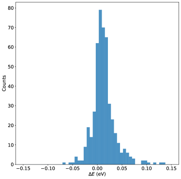
Figure 2: Differences of the DFT/MRCI(2) vertical excitation energies from those computed from the diagonalization of the DFT/MRCI Hamiltonian for the molecules in Thiel’s test set.

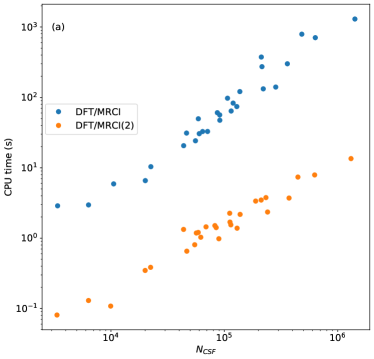
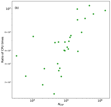
Figure 3: (a) Wall times for the diagonalization of the DFT/MRCI Hamiltonian matrix and DFT/MRCI(2) effective Hamiltonian matrix as a function of the total number of CSFs. (b) Ratio of the DFT/MRCI and DFT/MRCI(2) Hamiltonian diagonalization wall times as a function of the total number of CSFs. All calculations were performed using a single thread of an Intel Xeon Gold 6130 CPU @ 2.10 GHz.

To determine the accuracy of the DFT/MRCI(2) approximation, we consider the deviation of the eigenvalues $E_{I}^{[2]}$ of the effective Hamiltonian $\boldsymbol{\mathcal{H}}^{[2]}$ from the DFT/MRCI energies. To do so, vertical excitation energies were computed for the members of Thiel’s test set of 28 small-to-medium sized organic moleculesSchreiber et al. (2008). For each molecule in the set, four singly excited states per irrep were computed, resulting in a total of 472 excitation energies and accounting for states of both valence and Rydberg character. All calculations were performed using the aug-cc-pVDZ basisDunning (1989) and aug-cc-pVDZ-jkfit auxiliary basis.

Shown in Figure 2 are the differences, $\Delta E$, between the excitation energies obtained by diagonalizing the DFT/MRCI and effective DFT/MRCI(2) Hamiltonians. In general, excellent agreement is obtained, with a root mean squared deviation (RMSD) of 0.027 eV and a maximum absolute error of 0.138 eV being found for the 472 excited states considered. We also note that 99% of the DFT/MRCI(2) excitation energies are within 0.1 eV of the DFT/MRCI values. This value falls to 94% for an error bound of 0.05 eV. We thus conclude that DFT/MRCI(2) is, in general, an excellent approximation to the DFT/MRCI method.

As well as offering high precision (in comparison to the parent DFT/MRCI method), the DFT/MRCI(2) approximation also results in large computational savings by replacing the iterative diagonalization of the $N_{CSF}\times N_{CSF}$ DFT/MRCI Hamiltonian with the construction and diagonalization of the $N_{state}\times N_{state}$ DFT/MRCI(2) effective Hamiltonian $\boldsymbol{\mathcal{H}}_{DFT}^{[2]}$. Shown in Figure 3 (a) is a comparison of the CPU times for these steps for all molecules in the test set, shown as a function of the total number (summed across all irreps) of CSFs. We clearly see that the replacement of the DFT/MRCI Hamiltonian with the DFT/MRCI(2) effective Hamiltonian results in significant computational gains for all molecule in the test set. Indeed, even for the largest system considered (napthalene, 32 excited states), the construction and diagonalization of the effective Hamiltonian $\boldsymbol{\mathcal{H}}_{DFT}^{[2]}$ only requires around 10 seconds of CPU time. Note that this value accounts for all iterations of the reference space refinement. It is also insightful to consider the ratio of the CPU times for the diagonalization of the DFT/MRCI Hamiltonian and DFT/MRCI(2) effective Hamiltonian matrices. These values are shown plotted in Figure 3 (b) as a function of the total number of CSFs. The computational gains afforded by the DFT/MRCI(2) approximation are clearly seen, with speedups of around 80-100x being found for the largest molecules in the test set. It is noteworthy that the ratio of the timings of DFT/MRCI Hamiltonian and DFT/MRCI(2) effective Hamiltonian diagonalization steps grows with the size of the CSF basis, a result of the more lower scaling of the cost of effective Hamiltonian construction with the number of CSFs. We thus expect that even greater computational savings will be found as the size of the CSF basis grows.

Furthermore, it is important to note that for large CSF bases ($N_{CSF}>\sim 10^{6}$), a direct, configuration-driven algorithm becomes necessary in the iterative diagonalization of the DFT/MRCI Hamiltonian matrix, requiring a Hamiltonian build for every iteration. In contrast, the DFT/MRCI(2) effective Hamiltonian needs only to be constructed once in order to compute it’s eigenvalues and the first-order corrected wave functions. Thus, in such situations, one needs to multiply the ratio of the DFT/MRCI Hamiltonian and DFT/MRCI(2) effective Hamiltonian build times by the number of iterations required in the DFT/MRCI Hamiltonian diagonalization step to arrive at an estimate of the true computational savings afforded by the DFT/MRCI(2) approximation. As such, we predict that the computational savings afforded by the DFT/MRCI(2) approximation will reach up to three orders of magnitude when considering large systems.

IV.2 Comparison to p-DFT/MRCI

Recently, a new approximation to DFT/MRCI, termed p-DFT/MRCI, was introducedNeville and Schuurman (2021a). The idea underlying p-DFT/MRCI is to reduce the size of the CSF basis following the energy-based configuration selection by discarding superfluous configurations, as determined by a perturbative estimate of their contribution to the DFT/MRCI wave functions of interest. The DFT/MRCI Hamiltonian matrix is then built and diagonalized within the space spanned by the resulting pruned CSF basis, with the energetic contribution from the discarded CSFs being accounted for perturbatively. Considering their reliance on perturbation theories, it is worth while considering the relative performance and strengths of the p-DFT/MRCI and DFT/MRCI(2) methods.

First, we note that both methods use the Epstein-Nesbet partitioning of the Hamiltonian. In the case of DFT/MRCI(2), this is combined with GVVPT2 to arrive at an effective Hamiltonian formalism. In the p-DFT/MRCI approach, second-order RSPT is used in both the CSF pruning and perturbative energy correction steps (see Reference 11 for details). In both cases, however, the key quantities required to be computed are the B-vectors

$$\boldsymbol{B}_{I}=\langle\boldsymbol{\Omega}|\hat{H}^{DFT}|\Psi_{I}^{(0)}\rangle.$$ (30)

In p-DFT/MRCI, these are computed in, and form the bottleneck of, the pruning step, and are re-used in the application of the perturbative energy corrections. The calculation of the B-vectors is the bottleneck in a DFT/MRCI(2) calculation, being required to compute the effective Hamiltonian (see Equation 18). Thus, the calculation of the DFT/MRCI(2) effective Hamiltonian has essentially the same cost as the pruning step alone in a p-DFT/MRCI calculation. As such, a DFT/MRCI(2) calculation should always be computationally cheaper than the corresponding p-DFT/MRCI one.

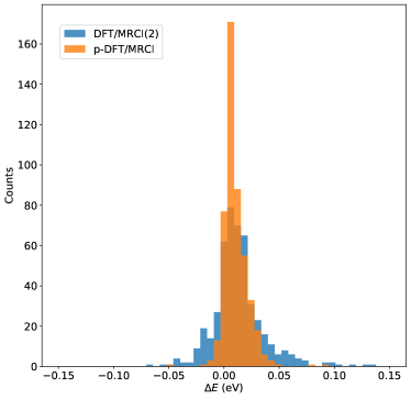
Figure 4: Differences of the DFT/MRCI(2) and p-DFT/MRCI vertical excitation energies from those computed from the diagonalization of the DFT/MRCI Hamiltonian for the molecules in Thiel’s test set. In the p-DFT/MRCI calculations, a pruning threshold of $\alpha_{p}=0.90$ was used.

We next consider the relative accuracies of DFT/MRCI(2) and p-DFT/MRCI relative to the original DFT/MRCI method. Shown in Figure 4 are the deviations $\Delta E$ of the DFT/MRCI(2) and p-DFT/MRCI excitation energies from the DFT/MRCI values for the molecules in Thiel’s test set. In the p-DFT/MRCI calculations, a pruning threshold of $\alpha_{p}=0.90$ was used (see Reference 11 for a definition of this quantity). It is found that DFT/MRCI(2) yields excitation errors of lower accuracy than p-DFT/MRCI. However, this deterioration of accuracy is slight, with the RMSDs increasing from 0.015 to 0.027 eV. Furthermore, similar maximum absolute errors of 0.086 and 0.138 eV are found for p-DFT/MRCI and DFT/MRCI(2), respectively. We thus conclude that DFT/MRCI(2) offers a very similar level of accuracy as p-DFT/MRCI but at reduced computational cost.

IV.3 Example calculations

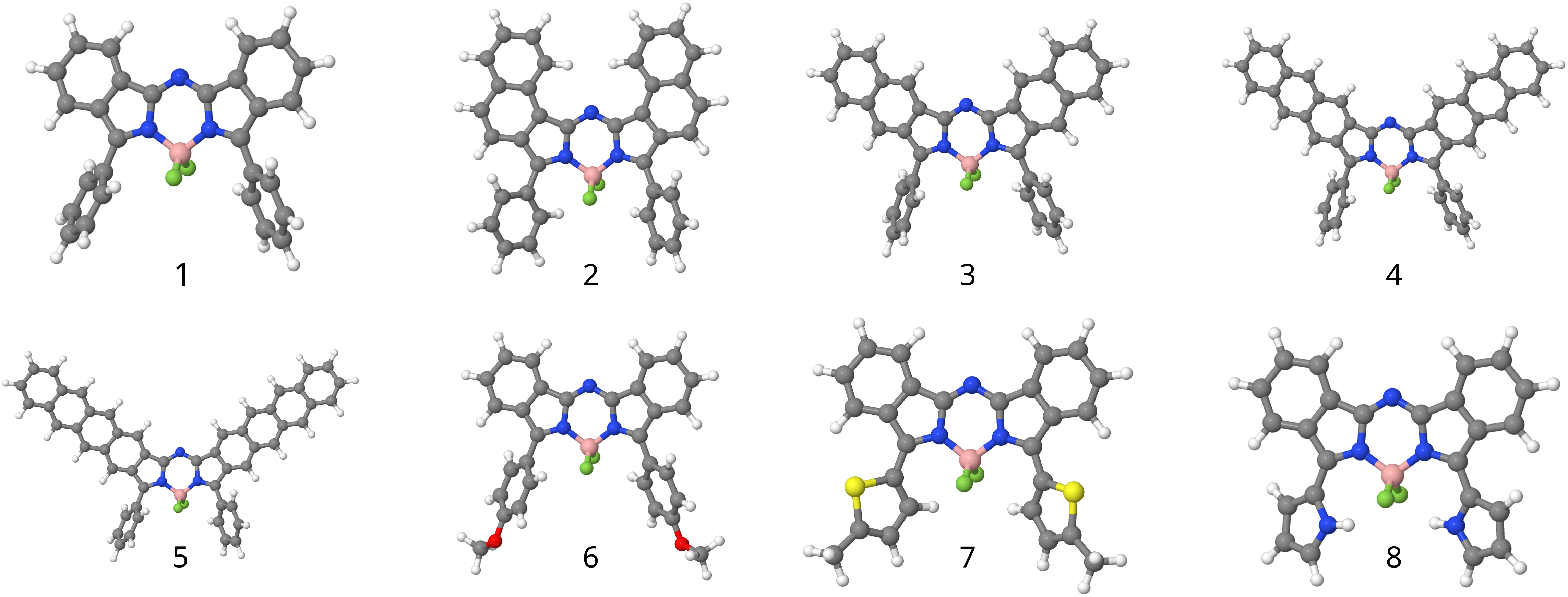
Figure 5: Set of aza-BODIPY molecules and numbering used in the example DFT/MRCI(2) calculations.

Having established the accuracy of the DFT/MRCI(2) approximation relative to the parent DFT/MRCI method, we now consider its application to a problem of real world interest: the $S_{1}$ vertical excitation energies of a range of aza-boron-dipyrromethane (aza-BODIPY) derivatives. This class of molecules are the subject of intense study given their use as near-infrared dyes in applications ranging from photovoltaics to bioimaging and photodynamic therapyErten-Ela et al. (2008); Rousseau et al. (2009); Whited et al. (2011); Flavin et al. (2011); Iehl et al. (2012); Zheng et al. (2008); Bouit et al. (2009); Didier et al. (2009); Coskun et al. (2007); Murtagh et al. (2009); Han et al. (2009); Shi et al. (2012); Killoran et al. (2002); Adarsh et al. (2010). The nine aza-BODIPY molecules shown in Figure 5 were chosen as representative examples. A recent study of these molecules by Berraud-Pache et al.Berraud-Pache et al. (2019) provides $S_{1}$ vertical excitation energies computed at the similarity transformed equation of motion coupled cluster with singles and doubles level of theory within the domain-based pair natural orbital approximation (DLPNO-STEOM-CCSD)Nooijen and Bartlett (1997); Riplinger and Neese (2013); Riplinger et al. (2013); Dutta et al. (2017, 2018). This allows us to make a meaningful comparison to excitation energies calculated at a near-benchmark ab initio level of theory.

As in Berraud-Pache et al.’s DLPNO-STEOM-CCSD calculations, the DFT/MRCI(2) calculations were performed using the def2-TZVP(-f) basis, along with the def2-universal-JKFIT auxiliary basis. In all calculations, an energy-based configuration selection threshold of $\delta E_{sel}=1.0$ E${}_{\text{h}}$ was used. The DLPNO-STEOM-CCSD calculations of Berraud-Pache et al. were performed using an implicit solvation model to simulate solvation in dicholoromethane. To account for this, the DFT/MRCI(2) calculations were performed in conjunction with the domain-decomposed COSMO (ddCOSMO) solvation modelCancès et al. (2013); Lipparini et al. (2013), using a dielectric constant of 8.93. The aza-BODIPY ground state minimum geometries were taken from Reference 52.

Table 1: $S_{1}$ vertical excitation energies, in units of eV, for the aza-BODIPY molecules calculated at the DFT/MRCI(2) and DLPNO-STEOM-CCSD levels of theory using def2-TZVP(-f) basis. DLPNO-STEOM-CCSD values are taken from Reference 52. A configuration selection threshold of $\delta E_{sel}=1.0$ E${}_{\text{h}}$ was used in all DFT/MRCI(2) calculations. Also given are the excitation energy differences, $\Delta E$, between the two levels of theory as well as the weight $|\langle\overline{\text{w}}\omega|\Psi_{0}\rangle|^{2}$ of the base configuration $\overline{\text{w}}$ in the DFT/MRCI(2) ground state wave functions.

Molecule	DFT/MRCI(2)	DLPNO-STEOM-CCSD	$\Delta E$	$|\langle\overline{\text{w}}\omega|\Psi_{0}\rangle|^{2}$
1	1.79	1.72	-0.07	0.88
2	1.63	1.60	0.03	0.87
3	1.40	1.44	0.04	0.84
4	1.10	1.23	-0.13	0.82
5	0.87	1.09	-0.22	0.80
6	1.73	1.64	0.09	0.88
7	1.61	1.55	0.06	0.88
8	1.59	1.58	0.01	0.87
9	1.61	1.52	0.09	0.88

Table 2: CSF basis dimensions, $N_{CSF}$, and CPU times (in units of seconds) for the aza-BODIPY DFT/MRCI(2) calculations. In all calculations, the def2-TZVP(-f) basis was used along with an energy-based configuration selection threshold of $\delta E_{sel}=1.0$ E${}_{\text{h}}$. All CPU times correspond to the use of a single thread of an Intel Xeon Gold 6130 CPU @ 2.10 GHz.

Molecule	$N_{CSF}$ / $10^{6}$	CPU time
1	2.4	72
2	6.9	170
3	7.1	142
4	17.5	308
5	42.7	636
6	3.5	99
7	2.7	86
8	1.3	53
9	1.5	49

Shown in Table 1 are the DFT/MRCI(2) $S_{1}$ vertical excitation energies alongside the reference DLPNO-STEOM-CCSD values for all nine aza-BODIPY molecules. In general, the agreement with the DLPNO-STEOM-CCSD results is excellent, with an RMSD of 0.10 eV being found. The largest deviations, -0.13 and -0.22 eV, occur for molecules 4 and 5, respectively. Interestingly, for these molecules, the DFT/MRCI(2) ground state wave function is found to contain significant contributions from non-base configurations: those with non-HF occupations. We find a significant contribution from multiple doubly-excited configurations, in particular those corresponding to excitation from the HOMO to LUMO KS MOs. As a measure of this, we also give in Table 1 the weights $|\langle\overline{\text{w}}\omega|\Psi_{0}\rangle|^{2}$ of the base configuration $\overline{\text{w}}$ for the DFT/MRCI(2) ground state $|\Psi_{0}\rangle$ of each molecule. This base configuration weight is smallest for molecules 4 and 5, taking values of 0.84 and 0.81, respectively. This result is in line with the those of Momeni and BrownMomeni and Brown (2015), in which the ground state wave functions of a large number of BODIPY molecules were found to contain significant contributions from doubly-excited configurations at the CASSCF level of theory. This suggests that a single reference method such as DLPNO-STEOM-CCSD might struggle to give a correct description of these systems, and may explain the larger discrepancy between the DFT/MRCI(2) and DLPNO-STEOM-CCSD excitation energies for these two molecules. A thorough investigation of this is, however, beyond the scope of the current paper, but may constitute an interesting avenue of future research.

Finally, we consider the computational efficiency of the DFT/MRCI(2) calculations. Although absolute timings are limited in meaning, being both hardware and implementation dependent, the CPU times for the example aza-BODIPY calculations do provide some insight into the high efficiency of the DFT/MRCI(2) method. These are shown, in Table 2 alongside the size of the final, converged CSF bases generated by the iteratively refined reference space. We note that these calculations were performed in serial on a single thread of an Intel Xeon Gold 6130 CPU @ 2.10 GHz. For the smallest calculations, molecules 8 and 9, with CSF basis sizes of $1.3\times 10^{6}$ and $1.5\times 10^{6}$, respectively, the cumulative cost of all steps involved in the DFT/MRCI(2) calculations took less one minute. In the largest calculation (molecule 5), the dynamic configuration selection algorithm (see Equation 23) generated an extremely large CSF basis of dimension $42.7\times 10^{6}$. However, the DFT/MRCI(2) calculation remained eminently tractable, requiring just over ten minutes in total.

V Conclusions and outlook

We have presented a new perturbative approximation to the DFT/MRCI method based on a combination of quasi-degenerate perturbation theory and the Epstein-Nesbet Hamiltonian partitioning. The resulting method, termed DFT/MRCI(2), replaces the iterative diagonalization of the DFT/MRCI Hamiltonian with the construction and full diagonalization of a small effective Hamiltonian matrix determined up to second-order in perturbation theory. This replacement of the full Hamiltonian diagonalization step results in orders of magnitude savings in terms of computational costs. Moreover, the resultant errors in the computed excitation errors are small, with an RMSD of 0.027 eV being found for an extensive set of excited states of the molecules in Thiel’s test setSchreiber et al. (2008).

In terms of potential applications, DFT/MRCI(2) seems ideally suited to situations in which either: (i) large numbers of excited states are required to be computed, and/or; (ii) potential energies (and potentially non-adiabatic couplings) are required at a large number of nuclear geometries. Scenario (i) is routinely encountered, e.g., in the calculation of X-ray absorption spectra for large molecules, where the number of core-excited states needed to be computed may number in the hundreds. Here, the DFT/MRCI(2) approximation will be advantageous due to: (a) a massive reduction in the cost associated with the (effective) Hamiltonian construction, as well as; (b) the complete obviation of the need to orthogonalize large numbers of wave function-sized vectors against each other that occurs in iterative diagonalization schemes. Scenario (ii) will occur if one is interested in the use of DFT/MRCI in quantum dynamics simulations. Here, the sheer reduction in computation cost afforded by the diagonalization of the DFT/MRCI(2) effective Hamiltonian instead the DFT/MRCI Hamiltonian imbues the method with much promise. Additionally, it will be trivial to pair DFT/MRCI(2) with a propagative block diagonalization diabatization scheme such as that detailed in Reference 9, allowing access to non-adiabatic coupling terms. As such, DFT/MRCI(2) offers much promise in the area of on-the-fly non-adiabatic quantum dynamics simulations. Both these areas of applications will be the subject of future work within our group.

References

- Grimme and Waletzke (1999) S. Grimme and M. Waletzke, J. Chem. Phys. 111, 5645 (1999), eprint https://doi.org/10.1063/1.479866, URL https://doi.org/10.1063/1.479866.
- Lyskov et al. (2016) I. Lyskov, M. Kleinschmidt, and C. M. Marian, J. Chem. Phys. 144, 034104 (2016), eprint https://doi.org/10.1063/1.4940036, URL https://doi.org/10.1063/1.4940036.
- Heil and Marian (2017) A. Heil and C. M. Marian, J. Chem. Phys. 147, 194104 (2017), eprint https://doi.org/10.1063/1.5003246, URL https://doi.org/10.1063/1.5003246.
- Marian et al. (2019) C. M. Marian, A. Heil, and M. Kleinschmidt, Wiley Interdiscip. Rev.: Comput. Mol. Sci. 9, e1394 (2019), eprint https://wires.onlinelibrary.wiley.com/doi/pdf/10.1002/wcms.1394, URL https://wires.onlinelibrary.wiley.com/doi/abs/10.1002/wcms.1394.
- Heil et al. (2018) A. Heil, M. Kleinschmidt, and C. M. Marian, J. Chem. Phys. 149, 164106 (2018), eprint https://doi.org/10.1063/1.5050476, URL https://doi.org/10.1063/1.5050476.
- Seidu et al. (2019) I. Seidu, S. P. Neville, M. Kleinschmidt, A. Heil, C. M. Marian, and M. S. Schuurman, J. Chem. Phys. 151, 144104 (2019), eprint https://doi.org/10.1063/1.5110418, URL https://doi.org/10.1063/1.5110418.
- Kleinschmidt et al. (2006) M. Kleinschmidt, J. Tatchen, and C. M. Marian, J. Chem. Phys. 124, 124101 (2006), eprint https://doi.org/10.1063/1.2173246, URL https://doi.org/10.1063/1.2173246.
- Kleinschmidt and Marian (2005) M. Kleinschmidt and C. M. Marian, Chem. Phys. 311, 71 (2005), ISSN 0301-0104, relativistic Effects in Heavy-Element Chemistry and Physics. In Memoriam Bernd A. Hess (1954–2004), URL https://www.sciencedirect.com/science/article/pii/S0301010404005634.
- Neville et al. (2020) S. P. Neville, I. Seidu, and M. S. Schuurman, J. Chem. Phys. 152, 114110 (2020), eprint https://doi.org/10.1063/1.5143126, URL https://doi.org/10.1063/1.5143126.
- Bracker et al. (2021) M. Bracker, C. M. Marian, and M. Kleinschmidt, The Journal of Chemical Physics 155, 014102 (2021), eprint https://doi.org/10.1063/5.0056182, URL https://doi.org/10.1063/5.0056182.
- Neville and Schuurman (2021a) S. P. Neville and M. S. Schuurman, Journal of Chemical Theory and Computation 17, 7657 (2021a), pMID: 34861111, eprint https://doi.org/10.1021/acs.jctc.1c00959, URL https://doi.org/10.1021/acs.jctc.1c00959.
- Epstein (1926) P. S. Epstein, Phys. Rev. 28, 695 (1926), URL https://link.aps.org/doi/10.1103/PhysRev.28.695.
- Nesbet and Hartree (1955) R. K. Nesbet and D. R. Hartree, Proceedings of the Royal Society of London. Series A. Mathematical and Physical Sciences 230, 312 (1955), eprint https://royalsocietypublishing.org/doi/pdf/10.1098/rspa.1955.0134, URL https://royalsocietypublishing.org/doi/abs/10.1098/rspa.1955.0134.
- Kirtman (1981) B. Kirtman, The Journal of Chemical Physics 75, 798 (1981), eprint https://doi.org/10.1063/1.442123, URL https://doi.org/10.1063/1.442123.
- Hirschfelder (1978) J. O. Hirschfelder, Chemical Physics Letters 54, 1 (1978), ISSN 0009-2614, URL https://www.sciencedirect.com/science/article/pii/0009261478856504.
- Certain and Hirschfelder (1970) P. R. Certain and J. O. Hirschfelder, The Journal of Chemical Physics 52, 5977 (1970), eprint https://doi.org/10.1063/1.1672896, URL https://doi.org/10.1063/1.1672896.
- Certain et al. (1970) P. R. Certain, J. O. Hirschfelder, and D. R. Dion, The Journal of Chemical Physics 53, 2992 (1970), eprint https://doi.org/10.1063/1.1674437, URL https://doi.org/10.1063/1.1674437.
- Wetmore and Segal (1975) R. W. Wetmore and G. A. Segal, Chem. Phys. Lett. 36, 478 (1975), ISSN 0009-2614, URL https://www.sciencedirect.com/science/article/pii/0009261475802843.
- Segal et al. (1978) G. A. Segal, R. W. Wetmore, and K. Wolf, Chem. Phys. 30, 269 (1978), ISSN 0301-0104, URL https://www.sciencedirect.com/science/article/pii/0301010478851246.
- Grimme (1996) S. Grimme, Chem. Phys. Lett. 259, 128 (1996), ISSN 0009-2614, URL https://www.sciencedirect.com/science/article/pii/0009261496007221.
- Olsen et al. (1988) J. Olsen, B. O. Roos, P. Jo/rgensen, and H. J. A. Jensen, J. Chem. Phys. 89, 2185 (1988), eprint https://doi.org/10.1063/1.455063, URL https://doi.org/10.1063/1.455063.
- BRANDOW (1967) B. H. BRANDOW, Rev. Mod. Phys. 39, 771 (1967), URL https://link.aps.org/doi/10.1103/RevModPhys.39.771.
- Löwdin and Goscinski (1971) P.-O. Löwdin and O. Goscinski, International Journal of Quantum Chemistry 5, 685 (1971), eprint https://onlinelibrary.wiley.com/doi/pdf/10.1002/qua.560050878, URL https://onlinelibrary.wiley.com/doi/abs/10.1002/qua.560050878.
- Lindgren (1974) I. Lindgren, Journal of Physics B: Atomic and Molecular Physics 7, 2441 (1974), URL https://doi.org/10.1088/0022-3700/7/18/010.
- Klein (1974) D. J. Klein, The Journal of Chemical Physics 61, 786 (1974), eprint https://doi.org/10.1063/1.1682018, URL https://doi.org/10.1063/1.1682018.
- Kvasnička (1977) V. Kvasnička, Application of Diagrammatic Quasidegenerate Rspt in Quantum Molecular Physics (John Wiley & Sons, Ltd, 1977), pp. 345–412, ISBN 9780470142554, eprint https://onlinelibrary.wiley.com/doi/pdf/10.1002/9780470142554.ch5, URL https://onlinelibrary.wiley.com/doi/abs/10.1002/9780470142554.ch5.
- Hose and Kaldor (1979) G. Hose and U. Kaldor, Journal of Physics B: Atomic and Molecular Physics 12, 3827 (1979), URL https://doi.org/10.1088/0022-3700/12/23/012.
- Shavitt and Redmon (1980) I. Shavitt and L. T. Redmon, The Journal of Chemical Physics 73, 5711 (1980), eprint https://doi.org/10.1063/1.440050, URL https://doi.org/10.1063/1.440050.
- Witek et al. (2002) H. A. Witek, Y.-K. Choe, J. P. Finley, and K. Hirao, Journal of Computational Chemistry 23, 957 (2002), eprint https://onlinelibrary.wiley.com/doi/pdf/10.1002/jcc.10098, URL https://onlinelibrary.wiley.com/doi/abs/10.1002/jcc.10098.
- Neville and Schuurman (2021b) S. Neville and M. Schuurman, GRaCI: General Reference Configuration Interaction (2021b), URL https://github.com/schuurman-group/graci.git.
- Sun et al. (2018) Q. Sun, T. C. Berkelbach, N. S. Blunt, G. H. Booth, S. Guo, Z. Li, J. Liu, J. D. McClain, E. R. Sayfutyarova, S. Sharma, et al., Wiley Interdiscip. Rev.: Comput. Mol. Sci. 8, e1340 (2018), eprint https://onlinelibrary.wiley.com/doi/pdf/10.1002/wcms.1340, URL https://onlinelibrary.wiley.com/doi/abs/10.1002/wcms.1340.
- Sun et al. (2020) Q. Sun, X. Zhang, S. Banerjee, P. Bao, M. Barbry, N. S. Blunt, N. A. Bogdanov, G. H. Booth, J. Chen, Z.-H. Cui, et al., J. Chem. Phys. 153, 024109 (2020), eprint https://doi.org/10.1063/5.0006074, URL https://doi.org/10.1063/5.0006074.
- Whitten (1973) J. L. Whitten, J. Chem. Phys. 58, 4496 (1973), eprint https://doi.org/10.1063/1.1679012, URL https://doi.org/10.1063/1.1679012.
- Feyereisen et al. (1993) M. Feyereisen, G. Fitzgerald, and A. Komornicki, Chem. Phys. Lett. 208, 359 (1993), ISSN 0009-2614, URL https://www.sciencedirect.com/science/article/pii/000926149387156W.
- Vahtras et al. (1993) O. Vahtras, J. Almlöf, and M. Feyereisen, Chem. Phys. Lett. 213, 514 (1993), ISSN 0009-2614, URL https://www.sciencedirect.com/science/article/pii/0009261493891517.
- Schreiber et al. (2008) M. Schreiber, M. R. Silva-Junior, S. P. A. Sauer, and W. Thiel, J. Chem. Phys. 128, 134110 (2008), eprint https://doi.org/10.1063/1.2889385, URL https://doi.org/10.1063/1.2889385.
- Dunning (1989) T. H. Dunning, J. Chem. Phys. 90, 1007 (1989), eprint https://doi.org/10.1063/1.456153, URL https://doi.org/10.1063/1.456153.
- Erten-Ela et al. (2008) S. Erten-Ela, M. D. Yilmaz, B. Icli, Y. Dede, S. Icli, and E. U. Akkaya, Organic Letters 10, 3299 (2008), pMID: 18588306, eprint https://doi.org/10.1021/ol8010612, URL https://doi.org/10.1021/ol8010612.
- Rousseau et al. (2009) T. Rousseau, A. Cravino, T. Bura, G. Ulrich, R. Ziessel, and J. Roncali, Chem. Commun. pp. 1673–1675 (2009), URL http://dx.doi.org/10.1039/B822770E.
- Whited et al. (2011) M. T. Whited, P. I. Djurovich, S. T. Roberts, A. C. Durrell, C. W. Schlenker, S. E. Bradforth, and M. E. Thompson, Journal of the American Chemical Society 133, 88 (2011), pMID: 21142032, eprint https://doi.org/10.1021/ja108493b, URL https://doi.org/10.1021/ja108493b.
- Flavin et al. (2011) K. Flavin, K. Lawrence, J. Bartelmess, M. Tasior, C. Navio, C. Bittencourt, D. F. O’Shea, D. M. Guldi, and S. Giordani, ACS Nano 5, 1198 (2011), pMID: 21291283, eprint https://doi.org/10.1021/nn102831x, URL https://doi.org/10.1021/nn102831x.
- Iehl et al. (2012) J. Iehl, J.-F. Nierengarten, A. Harriman, T. Bura, and R. Ziessel, Journal of the American Chemical Society 134, 988 (2012), pMID: 22148681, eprint https://doi.org/10.1021/ja206894z, URL https://doi.org/10.1021/ja206894z.
- Zheng et al. (2008) Q. Zheng, G. Xu, and P. Prasad, Chemistry – A European Journal 14, 5812 (2008), eprint https://chemistry-europe.onlinelibrary.wiley.com/doi/pdf/10.1002/chem.200800309, URL https://chemistry-europe.onlinelibrary.wiley.com/doi/abs/10.1002/chem.200800309.
- Bouit et al. (2009) P.-A. Bouit, K. Kamada, P. Feneyrou, G. Berginc, L. Toupet, O. Maury, and C. Andraud, Advanced Materials 21, 1151 (2009), eprint https://onlinelibrary.wiley.com/doi/pdf/10.1002/adma.200801778, URL https://onlinelibrary.wiley.com/doi/abs/10.1002/adma.200801778.
- Didier et al. (2009) P. Didier, G. Ulrich, Y. Mély, and R. Ziessel, Org. Biomol. Chem. 7, 3639 (2009), URL http://dx.doi.org/10.1039/B911587K.
- Coskun et al. (2007) A. Coskun, M. D. Yilmaz, and E. U. Akkaya, Organic Letters 9, 607 (2007), pMID: 17256867, eprint https://doi.org/10.1021/ol062867t, URL https://doi.org/10.1021/ol062867t.
- Murtagh et al. (2009) J. Murtagh, D. O. Frimannsson, and D. F. O’Shea, Organic Letters 11, 5386 (2009), pMID: 19883098, eprint https://doi.org/10.1021/ol902140v, URL https://doi.org/10.1021/ol902140v.
- Han et al. (2009) J. Han, A. Loudet, R. Barhoumi, R. C. Burghardt, and K. Burgess, Journal of the American Chemical Society 131, 1642 (2009), pMID: 19146412, eprint https://doi.org/10.1021/ja8073374, URL https://doi.org/10.1021/ja8073374.
- Shi et al. (2012) W.-J. Shi, J.-Y. Liu, and D. K. P. Ng, Chemistry – An Asian Journal 7, 196 (2012), eprint https://onlinelibrary.wiley.com/doi/pdf/10.1002/asia.201100598, URL https://onlinelibrary.wiley.com/doi/abs/10.1002/asia.201100598.
- Killoran et al. (2002) J. Killoran, L. Allen, J. F. Gallagher, W. M. Gallagher, and D. F. O’Shea, Chem. Commun. pp. 1862–1863 (2002), URL http://dx.doi.org/10.1039/B204317C.
- Adarsh et al. (2010) N. Adarsh, R. R. Avirah, and D. Ramaiah, Organic Letters 12, 5720 (2010), pMID: 21090576, eprint https://doi.org/10.1021/ol102562k, URL https://doi.org/10.1021/ol102562k.
- Berraud-Pache et al. (2019) R. Berraud-Pache, F. Neese, G. Bistoni, and R. Izsák, The Journal of Physical Chemistry Letters 10, 4822 (2019), pMID: 31386375, eprint https://doi.org/10.1021/acs.jpclett.9b02240, URL https://doi.org/10.1021/acs.jpclett.9b02240.
- Nooijen and Bartlett (1997) M. Nooijen and R. J. Bartlett, The Journal of Chemical Physics 107, 6812 (1997), eprint https://doi.org/10.1063/1.474922, URL https://doi.org/10.1063/1.474922.
- Riplinger and Neese (2013) C. Riplinger and F. Neese, The Journal of Chemical Physics 138, 034106 (2013), eprint https://doi.org/10.1063/1.4773581, URL https://doi.org/10.1063/1.4773581.
- Riplinger et al. (2013) C. Riplinger, B. Sandhoefer, A. Hansen, and F. Neese, The Journal of Chemical Physics 139, 134101 (2013), eprint https://doi.org/10.1063/1.4821834, URL https://doi.org/10.1063/1.4821834.
- Dutta et al. (2017) A. K. Dutta, M. Nooijen, F. Neese, and R. Izsák, The Journal of Chemical Physics 146, 074103 (2017), eprint https://doi.org/10.1063/1.4976130, URL https://doi.org/10.1063/1.4976130.
- Dutta et al. (2018) A. K. Dutta, M. Nooijen, F. Neese, and R. Izsák, Journal of Chemical Theory and Computation 14, 72 (2018), pMID: 29206453, eprint https://doi.org/10.1021/acs.jctc.7b00802, URL https://doi.org/10.1021/acs.jctc.7b00802.
- Cancès et al. (2013) E. Cancès, Y. Maday, and B. Stamm, The Journal of Chemical Physics 139, 054111 (2013), eprint https://doi.org/10.1063/1.4816767, URL https://doi.org/10.1063/1.4816767.
- Lipparini et al. (2013) F. Lipparini, B. Stamm, E. Cancès, Y. Maday, and B. Mennucci, Journal of Chemical Theory and Computation 9, 3637 (2013), pMID: 26584117, eprint https://doi.org/10.1021/ct400280b, URL https://doi.org/10.1021/ct400280b.
- Momeni and Brown (2015) M. R. Momeni and A. Brown, Journal of Chemical Theory and Computation 11, 2619 (2015), pMID: 26575559, eprint https://doi.org/10.1021/ct500775r, URL https://doi.org/10.1021/ct500775r.