Numerical and modeling error assessment of large-eddy simulation using direct-numerical-simulation-aided large-eddy simulation

Abstract

We study the numerical errors of large-eddy simulation (LES) in isotropic and wall-bounded turbulence. A direct-numerical-simulation (DNS)-aided LES formulation, where the subgrid-scale (SGS) term of the LES is computed by using filtered DNS data is introduced. We first verify that this formulation has zero error in the absence of commutation error between the filter and the differentiation operator of the numerical algorithm. This method allows the evaluation of the time evolution of numerical errors for various numerical schemes at grid resolutions relevant to LES. The analysis shows that the numerical errors are of the same order of magnitude as the modeling errors and often cancel each other. This supports the idea that supervised machine learning algorithms trained on filtered DNS data might not be suitable for robust SGS model development, as this approach disregards the existence of numerical errors in the system that accumulates over time. The assessment of errors in turbulent channel flow also identifies that numerical errors close to the wall dominate, which has implications for the development of wall models.

1 Introduction

DNS of most turbulent flows relevant for industrial applications is not tractable because the range of scales of motions in these flows is so large that the computational cost becomes prohibitive. In LES, the effect of the small scales on the larger ones is modeled through an SGS model, reducing the computational cost by several orders of magnitude. The accuracy of the representation of turbulent flows depends on both the performance or modeling capabilities of the choice of the SGS model, the adequacy of the LES resolution, and the numerical method employed to discretize the equations. In addition, the various sources of error can interact, which may lead to further complications in the validation of SGS models in LES. Given that accurate predictions are required in many engineering and scientific applications, a close assessment of LES numerical errors is crucial. This will also have implications for developing SGS models using supervised learning methods, which most often use filtered DNS data to train LES models without regarding the numerical errors.

Various SGS models have been introduced in the past decades such as the eddy-viscosity models [1, 2, 3, 4, 5], stochastic models [6, 7], similarity models [8, 9, 10], and mixed models [11, 12], among others. In addition, an important development in SGS modeling arose with the dynamic procedure [13, 14, 15], which allows optimization of parameters in the eddy-viscosity SGS models in accordance with the turbulent flow that is simulated. First works aiming to assess the accuracy of SGS models include the pioneering investigation by Clark et al. [8], who established the numerical study of decaying isotropic turbulence as a reference benchmark, although the grid resolutions and Reynolds numbers tested were highly constrained by the computational resources of the time. Since then, common benchmarks for LES have broadened to include simple hydrodynamic cases such as forced or decaying isotropic turbulence [4], rotating homogeneous turbulence [16], spatial or temporal mixing layers [17, 18] and plane turbulent channel flow [19, 13, 20, 21], among others. See Bonnet et al. [22] for an overview of cases for LES validation.

The validation cases mentioned above are representative of most LES error quantification, where the numerical error and the modeling error are not distinguished. Vreman et al. [23] was one of the first to quantify the modeling and discretization errors separately for various flow properties. In this analysis, modeling and numerical errors were found to be of comparable magnitude and could partially cancel each other. Further error analysis for LES was presented in Geurts and Fröhlich [24] in the context of the “subgrid-activity” parameter. More recently, Meyers et al. [25] differentiated the two errors and again showed that the partial cancellation of both sources can lead to coincidental accurate results. Along the same line, Meyers and Sagaut [26] studied the combined effect of discretization and model errors, and a further series of works resulted in the error-landscape-methodology framework reviewed by Meyers [27], where it is stressed that the determination of LES quality based on one single metric alone may provide misleading results. However, in these works, the LES errors are quantified as the error occurring in SGS models on a DNS grid by setting the filter size of the SGS grid to the LES grid size. As most SGS models for LES are not designed or expected to work in DNS grid resolutions, the error defined above may not be an accurate depiction of the true modeling error observed in LES grid resolutions. Moreover, this method is able to assess SGS models when there is a clearly defined filter size, which is not straightforward for anisotropic and unstructured grids [28]. Ideally, the modeling error would compare a filtered DNS solution in an LES grid with the LES solution. This can be made possible by first quantifying the correct numerical error for an LES using explicitly filtered LES.

Previous works on explicitly filtered LES include the study of Winckelmans et al. [29], who investigated a two-dimensional explicitly filtered isotropic turbulence and channel flow LES to evaluate various mixed subgrid/subfilter scale models. Stolz et al. [30] implemented the three-dimensional filtering schemes of Vasilyev et al. [31] by using an approximate deconvolution model for the convective terms in the LES equations. Lund [32] applied two-dimensional explicit filters to a channel flow and evaluated the performance of explicitly filtered versus implicitly filtered LES. Gullbrand and Chow [33] attempted the first grid-independent solution of the LES equations with explicit filtering. Bose et al. [34] further investigated the grid independence of explicitly filtered LES with a three-dimensional filter for turbulent channel flows. The recent works of Bae and Lozano-Durán [35, 36] introduce a DNS-aided LES (DAL) framework using explicitly filtered LES that computes the exact SGS stress term in the absence of commutation errors from filtered DNS data.

From a different perspective, machine-learning-based SGS models trained using high-fidelity data, typically DNS, have recently emerged (see reviews [37, 38, 39, 40]). SGS models have been developed in several canonical and complex flows, including two-dimensional homogeneous isotropic turbulence [41, 42], three-dimensional forced and [43, 44, 45, 46] decaying [47, 48] isotropic turbulence, turbulent channel flow [49, 50, 51], and flow over an aircraft [52]. A majority of the research utilizes a supervised learning framework, where the model is trained to produce accurate SGS stresses obtained from DNS (or filtered DNS) data, and is often based on single-step target values to limit computational challenges in minimizing the model prediction error. Therefore, it is important to differentiate between a priori and a posteriori testing for these models. While the model might perform well in a priori testing, a posteriori testing is performed by integrating the LES equations in time. Due to the single-step cost function as well as the discrepancy in the filtered Navier-Stokes and LES equations, the resulting machine-learned model is not trained to compensate for the discrepancies between DNS and LES and the compounding (numerical and modeling) errors. The issue of inconsistency in data-driven SGS models has been exposed by studies that performed a posteriori testing [53, 49, 48]. Thus, in order to account for the discrepancies between DNS and LES in machine-learning-based model development, a systematic understanding of the different errors associated with LES SGS modeling is necessary.

It is the aim of this paper to introduce a framework that will allow the evaluation of the time evolution of numerical errors in LES. For that purpose, we introduce a method that produces zero modeling error using the DAL framework [35, 36] as a method to define separate numerical and modeling errors. Our goal is to assess the errors for unbounded and wall-bounded turbulent flows using this methodology. In particular, for wall-bounded flows, the wall-normal dependency of errors in LES will be investigated.

The paper is organized as follows. In Section 2, the filtered Navier-Stokes equations are compared to the traditional LES equations to clearly define numerical error, and the DAL framework is introduced. We then introduce the numerical experiments in Section 3, where we evaluate the numerical errors for forced isotropic turbulence and turbulent channel flows. Finally, we conclude the paper in Section 4.

2 Zero-modeling-error formulation

2.1 Filtered Navier-Stokes equations and large-eddy simulation equations

The incompressible Navier-Stokes equations are given by

$${\frac{\partial{u}_{i}}{\partial t}}+{\frac{\partial{u}_{i}{u}_{j}}{\partial x_{j}}}=-\frac{1}{\rho}{\frac{\partial{p}}{\partial x_{i}}}+\nu{\frac{\partial^{2}{u}_{i}}{\partial x_{j}\partial x_{j}}},\quad{\frac{\partial{u}_{i}}{\partial x_{i}}}=0,$$ (1)

where the velocity components are represented by ${u}_{i}$ for $i=1,2,3$ (or equivalently $u$, $v$, and $w$) for the directions $x_{i}$ ($x$, $y$, and $z$), $\rho$ is the fluid density, $\nu$ is the kinematic viscosity, and $p$ is the pressure. As LES is formally derived from the filtered Navier-Stokes equations, we define a filter operator on a variable $\phi$ in integral form

$$\bar{\phi}(\boldsymbol{x})=\int_{\Omega}G(t,\boldsymbol{x},\boldsymbol{x^{\prime}})\phi(\boldsymbol{x^{\prime}})\mathrm{d}\boldsymbol{x^{\prime}},$$ (2)

where $\boldsymbol{x}=(x_{1},x_{2},x_{3})$, $G$ is the filter kernel, and $\Omega$ is the domain of integration. When Eq. (1) is filtered with Eq. (2), the resulting equations are

$$\overline{\frac{\partial{u}_{i}}{\partial t}}+\overline{\frac{\partial{u}_{i}{u}_{j}}{\partial x_{j}}}=-\frac{1}{\rho}\overline{\frac{\partial{p}}{\partial x_{i}}}+\nu\overline{\frac{\partial^{2}{u}_{i}}{\partial x_{j}\partial x_{j}}},\quad\overline{\frac{\partial{u}_{i}}{\partial x_{i}}}=0.$$ (3)

However, in LES, we have access to the filtered velocity quantities $\bar{u}_{i}$ and not the full flow field $u_{i}$. In order to be able to solve Eq. (3) for a practical LES applications, the order of the filter and the differentiation operator must be inverted such that the equations become

$${\frac{\partial\bar{u}_{i}}{\partial t}}+{\frac{\partial\overline{\bar{u}_{i}\bar{u}_{j}}}{\partial x_{j}}}=-\frac{1}{\rho}{\frac{\partial\bar{p}}{\partial x_{i}}}+\nu{\frac{\partial^{2}\bar{u}_{i}}{\partial x_{j}\partial x_{j}}}-\frac{\partial\mathcal{T}_{ij}}{\partial x_{j}}+\delta^{\text{num}}_{i},\quad{\frac{\partial\bar{u}_{i}}{\partial x_{i}}}+\delta^{\text{num}}=0,$$ (4)

where $\delta^{\text{num}}_{i}$ and $\delta^{\text{num}}$ are the commutation error due to the inversion of the order of operators. In traditional LES, the commutation error is often neglected or assumed to be zero regardless of the choice of filter and differentiation operator. However, in most numerical methods used for LES, these commutation errors are not negligible even with the use of commutative filters [54] as the commutation of the two operators is guaranteed only up to a finite order. Here, we retain $\delta^{\text{num}}_{i}$ and $\delta^{\text{num}}$ to signify the difference between the formulations in Eq. (3) and Eq. (4). The term $\mathcal{T}_{ij}=\overline{u_{i}u}_{j}-\overline{\bar{u}_{i}\bar{u}_{j}}$ is the SGS stress tensor, which is modeled through an SGS model in LES. At each time step, the effect of using an SGS model can be characterized as $\delta^{\text{mod}}_{i}=\partial/\partial x_{j}\left(\mathcal{T}_{ij}^{\text{SGS}}-\mathcal{T}_{ij}\right)$, where $\mathcal{T}_{ij}^{\text{SGS}}$ is the modeled SGS stress tensor given by the choice of SGS model. In this paper, we will categorize the time-integrated effect of $\delta^{\text{num}}_{i}$ and $\delta^{\text{num}}$ as the numerical error, $\mathcal{E}^{\text{num}}$ in the absence of $\delta_{i}^{\text{mod}}$.

2.2 Zero-modeling error through DNS-aided LES

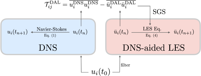
Figure 1: Schematic of DAL. The SGS stress tensor $\mathcal{T}_{ij}^{\text{DAL}}$ is computed at each time step from the DNS flow field at the same time step and then applied to the LES equations.

One possible way of enforcing zero modeling error in LES is by using an exact SGS model that can be produced by running a DNS concurrently. That is, starting from an initial DNS velocity field $u^{\text{DNS}}_{i}(t_{0})$ and filtering it, we can compute the initial condition $\bar{u}^{\text{DAL}}_{i}(t_{0})$ for the DAL simulations such that $\overline{u^{\text{DNS}}_{i}}(t_{0})=\bar{u}^{\text{DAL}}_{i}(t_{0})$. At any given time step $t_{n}$ of the DAL, the exact SGS stress tensor $\mathcal{T}_{ij}$ can be given by the DNS at the same time step $t_{n}$, i.e.,

$$\mathcal{T}_{ij}^{\text{DAL}}(t_{n})=\overline{u^{\text{DNS}}_{i}(t_{n})u^{\text{DNS}}_{j}(t_{n})}-\overline{\bar{u}^{\text{DAL}}_{i}(t_{n}){\bar{u}^{\text{DAL}}}_{j}(t_{n})}.$$ (5)

A schematic of the proposed method is given in Figure 1. Note that this would be not possible for traditional implicitly filtered LES due to the lack of an explicit filter operator. In the absence of numerical (commutation) error, the filtered DNS and DAL solutions will be identical, thus the name zero modeling error. However, in the presence of numerical error, the solutions of $\overline{u^{\text{DNS}}_{i}}$ and $\bar{u}_{i}^{\text{DAL}}$ will diverge from the integrated effect of $\delta_{i}^{\text{num}}$, and the difference in the filtered DNS and DAL solution will provide a measure for the numerical error of the simulation without the presence of modeling error in a grid relevant to LES.

3 Error evaluation in LES

We consider two test cases, forced isotropic turbulence and turbulent channel flow, to evaluate the numerical and modeling errors of LES. We quantify the error in the LES flow fields as the $L_{2}$ error of the filtered DNS and LES velocity fields,

$$\mathcal{E}^{\text{tot}}(t)= \bigg{[}\frac{1}{L_{x}L_{y}L_{z}}\iiint\sum_{i=1}^{3}\left(\overline{u_{i}^{\text{DNS}}}(t)-\bar{u}_{i}^{\text{LES}}(t)\right)^{2}\mathrm{d}x\,\mathrm{d}y\,\mathrm{d}z\bigg{]}^{1/2},$$ (6)

where $L_{x,y,z}$ is the length of the domain in the corresponding direction. The error $\mathcal{E}^{\text{tot}}$ can be seen as a combination of the numerical and modeling error by considering the square-root of the integrand of Eq. (6) as

$$\overline{u_{i}^{\text{DNS}}}(t)-\bar{u}_{i}^{\text{LES}}(t)=\left(\overline{u_{i}^{\text{DNS}}}(t)-\bar{u}_{i}^{\text{DAL}}(t)\right)+\Big{(}\bar{u}_{i}^{\text{DAL}}(t)-\bar{u}_{i}^{\text{LES}}(t)\Big{)},$$ (7)

where we define the numerical error as

$$\mathcal{E}^{\text{num}}(t)=\left[\frac{1}{L_{x}L_{y}L_{z}}\iiint\sum_{i=1}^{3}\left(\overline{u_{i}^{\text{DNS}}}(t)-\bar{u}_{i}^{\text{DAL}}(t)\right)^{2}\mathrm{d}x\,\mathrm{d}y\,\mathrm{d}z\right]^{1/2}.$$ (8)

In essence, the numerical error quantifies the error due to the filter operator.

In the case of channel flow, we also quantify a wall-normal distance dependent error

$$\mathcal{E}^{\text{tot}}_{y}(y,t)=\left[\frac{1}{L_{x}L_{z}}\iint\sum_{i=1}^{3}\left(\overline{u_{i}^{\text{DNS}}}(y,t)-\bar{u}_{i}^{\text{LES}}(y,t)\right)^{2}\mathrm{d}x\,\mathrm{d}z\right]^{1/2},$$ (9)

where $y$ is the wall-normal direction. An analogous $y$-dependent numerical error can be defined as $\mathcal{E}^{\text{num}}_{y}$.

It is worth remarking the fact that if an SGS model is able to counteract the numerical errors with the modeling errors such that $\left(\overline{u_{i}^{\text{DNS}}}(t)-\bar{u}_{i}^{\text{DAL}}(t)\right)=-\Big{(}\bar{u}_{i}^{\text{DAL}}(t)-\bar{u}_{i}^{\text{LES}}(t)\Big{)}$, the total error is zero. Thus, not only does the DAL formulation provide a method to evaluate errors, it can be used to inform future SGS models. However, SGS models are not expected to provide the correct closure term in an instantaneous manner. Rather, the goal of LES is to obtain the correct statistics of the system. Thus, computing instantaneous modeling errors does not align with the goal of LES and SGS modeling and will not be considered in this paper.

3.1 Forced isotropic turbulence

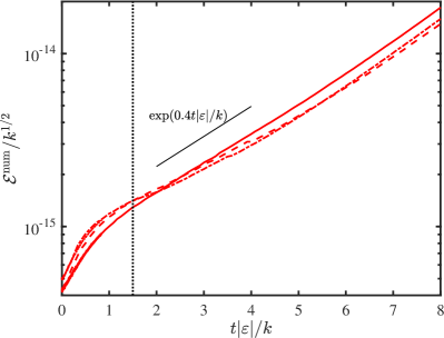
(a)

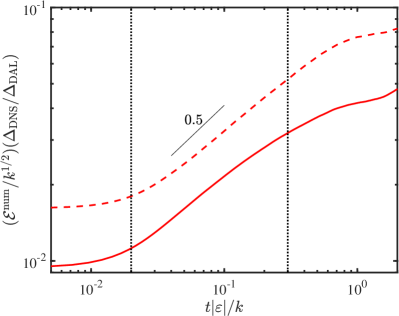
(b)

Figure 2: (a) Time evolution of the numerical error $\mathcal{E}^{\text{num}}$ using dealiased Fourier discretization in space and the Fourier cutoff filter for grid resolutions $32^{3}$ ( ), $64^{3}$ ( ), and $128^{3}$ ( ). Vertical lines ( ) divide the initial response region and growth region. (b) Time evolution of the numerical error $\mathcal{E}^{\text{num}}$ using a second-order finite difference in space and downsampling for grid resolutions $80^{3}$ ( ) and $48^{3}$ times ( ). Vertical lines ( ) divide the initial response region, growth region, and saturation region.

To demonstrate the method given in section 2.2 provides zero modeling error and evaluate modeling error, we first perform a simulation of forced isotropic turbulence using a dealiased Fourier discretization in space in a triply periodic domain of size $2\pi^{3}$ and advanced in time using a fourth-order Runge-Kutta time stepping method. A linear forcing [55], $f_{i}=Au_{i}$, is applied with $A=0.45$. The DNS is performed using a $256^{3}$ mesh at $Re_{\lambda}\approx 100$. Three DAL (section 2.2) cases with grid resolution of $32^{2}$, $64^{3}$ and $128^{3}$ are performed with the filter operator given by a sharp Fourier cutoff filter at the largest wavenumber resolvable by the LES grid. The LES simulations are run with the same time-step size as DNS to take advantage of the DAL formulation without interpolation in time. The initial condition for the numerical experiment was taken from a separate DNS after transients. The errors are normalized by the square-root of the turbulence kinetic energy $k$, and the time is given in integral times $k/|\varepsilon|$, where $\varepsilon$ is the dissipation rate.

We evaluate the numerical error using DAL. Since DAL can be thought of as supplying the exact SGS model that produces zero modeling error, the difference between the filtered DNS flow field and the DAL flow field can be considered the numerical error as defined in the beginning of section 2.1. The sharp Fourier cutoff filter used in the simulations commutes with the derivative operator in Fourier space, which gives, in theory, zero numerical error. In practice, the numerical error is zero only up to machine precision, and the resulting small perturbations in the velocity profile will grow exponentially following the leading Lyapunov exponent of the Navier-Stokes equation until it reaches saturation [56]. The Lyapunov exponent $\lambda$ represents the rate of separation, such that the error grows proportional to $\exp(\lambda t)$, and its reciprocal is closely related to the predictability horizon of a chaotic solution, such as solutions to the Navier-Stokes equations. Thus, DAL solution should give $\mathcal{E}^{\text{num}}\approx 0$ initially with a small exponential growth rate to ensure that this formulation is effective.

In Figure 2(a), we plot $\mathcal{E}^{\text{num}}(t)$ for the cases considered. As expected, the error is initially $O(10^{-15})$ for all LES grid resolutions, with the error following a linear curve, known as the initial response, until $t|\varepsilon|/k\approx 1.5$. Then, the error grows exponentially in time with an exponential growth rate, or the Lyapunov exponent, of $\lambda k/|\varepsilon|\approx 0.4$. This demonstration shows that for short times, the two flow fields can be considered identical (the error will be less than $10^{-10}$ for 30 integral times), and thus, the modeling error evaluated from DAL flow fields is zero in the absence of numerical error.

We repeat the previous experiment using a second-order finite difference staggered discretization in space and advanced in time using a third-order Runge-Kutta time-stepping method. The same linear forcing is applied using a $240^{3}$ mesh. The DAL cases are three and five times coarser than the DNS case in all three spatial directions, i.e., computed on a $80^{3}$ and $48^{3}$ mesh. Due to the numerical method of the simulation, there is no filter operator that maps a velocity field of a DNS grid to a smaller LES grid and commutes with the differentiation matrix (see Appendix A). An example of a case with the LES grid equal to the DNS grid is given in Bae and Lozano-Durán [36] for a differential filter [57] utilizing the extension method [35, 36]. However, for practical applications, LES should reduce the computational cost by using a low pass filter and a smaller computational domain. Here, we utilize a down-sampling method where the velocity field at a certain point of the LES is the same as the (interpolated) DNS velocity field at the same point.

The numerical error $\mathcal{E}^{\text{num}}$ as a function of time is given in figure 2(b). Unlike the case using Fourier discretization where the differentiation operator commutes with the Fourier-cutoff filter, the down-sampling does not commute with the second-order finite-difference operation. The error is much larger from the first time step, assuming a polynomial growth with a growth factor of $0.4$ until it reaches saturation. Unlike the previous case, the initial error is too large and the gap between the initial and fully saturated error is too small to develop an exponential growth region. Instead, the polynomial growth rate shows how the initial error develops.

3.2 Channel flow

We perform a set of plane turbulent channel simulations at friction Reynolds number $Re_{\tau}=u_{\tau}h/\nu\approx 180$ and $550$, where $h$ is the channel half-height and $u_{\tau}$ is the friction velocity at the wall. The simulations are computed with a staggered second-order finite difference [58] and a fractional-step method [59] with a third-order Runge-Kutta time-advancing scheme [60]. The code has been validated in previous studies in turbulent channel flows [61, 62, 63]. The size of the channel is $2\pi h\times 2h\times\pi h$ in the $x$, $y$ and $z$ directions, which are the streamwise, wall-normal, and spanwise directions, respectively. It has been shown that this domain size is sufficient to accurately predict one-point statistics for $Re_{\tau}$ up to 4200 [64]. Periodic boundary conditions are imposed in the streamwise and spanwise directions, and the flow is driven by imposing a constant mean pressure gradient.

The DNS grid resolution utilizes $192\times 120\times 96$ grid points for the $Re_{\tau}\approx 180$ case and $510\times 300\times 510$ grid points for the $Re_{\tau}\approx 550$ case in the three spatial directions. The streamwise and spanwise directions are uniform with $\Delta_{x}^{+}\approx 6$ and $\Delta_{z}^{+}\approx 6$ or $3$, where the superscript $+$ denotes wall units given by $\nu$ and $u_{\tau}$. Non-uniform meshes are used in the normal direction, with the grid stretched toward the wall according to a hyperbolic tangent distribution. The height of the first grid cell at the wall is $\Delta_{y}^{+}\approx 0.2$ for both cases. The DAL cases are either three or five times coarser than the DNS case in all three spatial directions. Similar to the forced isotropic turbulence case, we utilize a down-sampling method where the velocity field at a certain point of the LES is the same as the (interpolated) DNS velocity field at the same point. The details of the simulations are given in Table 1.

Case	Method	$Re_{\tau}$	$\Delta_{x}^{+}$	$\min(\Delta_{y}^{+})$	$\max(\Delta_{y}^{+})$	$\Delta_{z}^{+}$
CH180DNS	DNS	$186$	6.1	0.19	8.2	6.1
CH180DAL3	DAL	$186$	18.3	0.61	24.3	18.3
CH550DNS	DNS	$547$	6.7	0.21	9.6	3.4
CH550DAL3	DAL	$547$	20.2	0.66	28.7	10.1
CH550DAL5	DAL	$547$	33.6	0.97	49.5	16.8
CH550DSM3	DSM	$547$	20.2	0.66	28.7	10.1
CH550AMD3	AMD	$547$	20.2	0.66	28.7	10.1
CH550NM3	NM	$547$	20.2	0.66	28.7	10.1

Table 1: Tabulated list of cases for the channel flow case. Cases are named as CH[$Re_{\tau}$][Method][Coarsening Factor], where method is either DNS or DAL and coarsening factor is the ratio of grid points from DNS to DAL in one spatial direction.

(a)

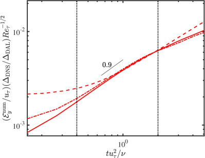
(b)

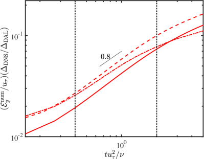
(c)

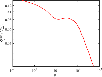
(d)

Figure 3: Time evolution of the (a) integrated numerical error $\mathcal{E}^{\text{num}}$ and wall-normal distance dependent numerical error $\mathcal{E}^{\text{num}}_{y}$ at (b) $y^{+}\approx 15$ and (c) $y/h\approx 1$ for CH180DAL3 ( ), CH550DAL3 ( ), and CH550DAL5 ( ). Vertical lines ( ) divide the initial response region, growth region, and saturation region. (d) $\mathcal{E}^{\text{num}}_{y}$ normalized with the mean velocity profile as a function of wall-normal height at $tu_{\tau}^{2}/\nu\approx 1$ for CH550DAL3.

In order to evaluate the numerical error, we use the same approach as in section 3.1 and supply the SGS stress term using DAL for the three different cases. Figure 3(a) shows the evolution of the integrated numerical error as a function of time. When the error is normalized with $\Delta_{\text{DNS}}/\Delta_{\text{DAL}}$, we see that the error evolution of the three cases collapses. The linear dependence of the error on grid resolution and its independence on Reynolds number is similar to the LES error scalings found in Lozano-Durán and Bae [21]. This study did not distinguish between modeling and numerical errors and considered errors in resulting statistics. However, this shows that either the numerical errors are dominant in the total LES error or the modeling error is proportional to the numerical error, demonstrating that numerical errors are a significant source of error in LES.

For all three cases, after the initial linear growth, the errors assume a polynomial growth with a growth rate of 0.8, until saturation. This growth rate is larger than that observed in the forced isotropic turbulence case. The faster growth in error can be attributed to the non-uniform mesh in the wall-normal direction and, incidentally, the modifications in the Poisson solver, which contribute towards additional sources of numerical error.

Figures 3(b) and (c) show $\mathcal{E}^{\text{num}}_{y}$ for a given time at different wall-normal heights, $y^{+}\approx 15$ and $y/\delta=1$. The linear dependence on the factor $\Delta_{\text{DNS}}/\Delta_{\text{DAL}}$ is true for all wall-normal heights, similar to the integrated error. The growth rates are similar for the two wall-normal heights, with the error accumulating slightly slower in the outer region, compared to the error at $y^{+}\approx 15$. This shows that the numerical error will accumulate faster closer to the wall. Additionally, the errors are weakly dependent on Reynolds number close to the wall, but become independent of Reynolds number away from the wall. Thus, the relative error close to the wall will increase with Reynolds number but stay constant with Reynolds number in the outer region. Moreover, the relative $y$-dependent numerical error at each wall-normal height is given in figure 3(d). While only one time step is shown, all temporal locations show similar trends as a function of wall-normal distance. This shows that the relative numerical error is the largest close to the wall and decreases with distance from the wall. This large and fast accumulation of errors in the near-wall region is known to be problematic for SGS models and in particular for wall models for LES.

Finally, we plot the modeling and total errors for the DSM and AMD model as well as the NM case in figure 4. The errors show that the AMD model has the largest modeling error $\mathcal{E}_{mod}$, followed by the DSM and the NM case. However, the total error $\mathcal{E}_{tot}$ shows the smallest error for the AMD case, followed by the DSM and NM. This demonstrates that the modeling error and the numerical error cancel each other, as widely accepted in the literature.

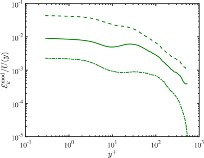
(a)

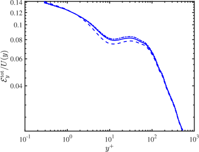
(b)

Figure 4: (a) $\mathcal{E}^{\text{mod}}_{y}$ and (b) $\mathcal{E}^{\text{tot}}_{y}$ normalized with the mean velocity profile as a function of wall-normal height at $tu_{\tau}^{2}/\nu\approx 1$ for CH550DSM3 ( ), CH550AMD3 ( ), and CH550NM3 ( ).

4 Conclusions

Large-eddy simulation has become a viable tool in performing simulations of turbulent flow for industrial and engineering applications. In order for LES to be regarded as a useful tool, the errors associated with it must be carefully studied. In particular, the errors associated with the numerical method and the choice of SGS model must be clearly distinguished and evaluated at grid resolutions relevant to practical LES applications. Moreover, for wall-bounded flows, it is important to evaluate the error as a function of wall-normal distance to account for near-wall effects.

In this paper, we introduce a formulation that allows the accurate assessment of numerical errors at grid resolutions typical of LES. DNS-aided LES is used to compute exact SGS stress terms in the absence of numerical error; that is, by running a DNS and LES with the equivalent initial condition, the DNS flow field at each time step is used to generate the exact SGS stress term for the corresponding LES flow field. This requires an explicit filter operator which is often lacking in traditional LES. DAL allows the evaluation of numerical errors as a function of time. Moreover, it allows the distinction of numerical and modeling errors for LES, which is often not straightforward.

Using this method, we compute the numerical errors of two cases: forced isotropic turbulence and turbulent channel flow. The evaluation of numerical errors of the Fourier discretization shows that the errors are machine precision zero, as expected. This also verifies that DAL indeed produces zero modeling error. In the case of numerical error for the finite difference case, the error follows a polynomial growth until saturation. The growth rate is indicative of how the LES solution is correlated to the corresponding DNS solution. The results verify that the numerical errors are largest closer to the wall. Furthermore, it also shows that numerical errors and modeling errors partially counteract each other. The findings imply that SGS models are not expected to perform well in all numerical methods and will perform better when coupled with numerical methods where the numerical errors are counterbalanced with the modeling errors. In particular, supervised learning SGS models trained on filtered DNS data do not account for numerical errors, and thus do not perform as expected in a posteriori testing. The latter observation also has implications for wall modeling in LES, in which wall models become sensitive to the flow details close to the wall where the numerical errors are the largest.

The method introduced here can be helpful in two main directions. Firstly, the method can inform the development of new SGS models in conjunction with a target numerical method such that the effect of counterbalancing the numerical and modeling errors is maximized. Since the method here provides the numerical errors as a function of space and time, this information can be used to develop SGS models specifically designed to cancel numerical errors. Secondly, the method can similarly aid in the development and assessment of wall models, which remains a pacing item to achieve practical LES.

Appendix A Commutation of filter operator for finite difference

For the filter operator to commute with the differentiation operator numerically, we need, in matrix form,

$$D^{\text{LES}}F\vec{u}=FD^{\text{DNS}}\vec{u},$$ (10)

where a nonzero matrix $F\in\mathbb{R}^{N\times mN}$ is the filter matrix, $D^{\text{DNS}}\in\mathbb{R}^{mN\times mN}$ and $D^{\text{LES}}\in\mathbb{R}^{N\times N}$ are the one-dimensional differentiation matrix for DNS and LES respectively. The factor $m$ denotes the ratio between the DNS and LES grid sizes, and for practical cases, $m>1$. For simplicity, we consider the central finite difference in a uniform grid, which gives

$$D^{\text{DNS}}_{i,j}=\begin{cases}1/\Delta,&i=j+1\\ -1/\Delta,&i=j-1\\ 0,&\text{otherwise}\end{cases},\quad D^{\text{LES}}_{i,j}=\begin{cases}1/m\Delta,&i=j+1\\ -1/m\Delta,&i=j-1\\ 0,&\text{otherwise}\end{cases},$$ (11)

where $\Delta$ is the grid size for DNS.

Solving Eq. (10) as $F=D^{\text{LES}-1}FD^{\text{DNS}}$, we get

$$F_{i,j}=\begin{cases}\displaystyle{m\sum_{k=(i+1)/2}^{N/2}\left(-F_{2k,j-1}+F_{2k,j+1}\right)},&i\text{ odd}\\ \displaystyle{m\sum_{k=1/2}^{(i-1)/2}\left(F_{2k,j-1}-F_{2k,j+1}\right)},&i\text{ even}\end{cases}$$ (12)

We can rewrite this equation as a linear equation $M\vec{f}=\vec{f}$ by transforming matrix $F$ as a vector $\vec{f}\in\mathbb{R}^{mN^{2}}$, such that $\vec{f}_{mN(i-1)+j}=F_{i,j}$. Thus, there exists a filter that commutes with the finite difference if and only if $M$ has an eigenvalue of unity. While there may be a specific choice of $m$ and $N$ such that this is possible (e.g. $m=1$), for an arbitrary grid, this is not always true.

References

- Smagorinsky [1963] J. Smagorinsky, General circulation experiments with the primitive equations, Mon. Weather Rev. 91 (1963) 99–164.
- Schumann [1975] U. Schumann, Subgrid scale model for finite difference simulations of turbulent flows in plane channels and annuli, J. Comput. Phys. 18 (1975) 376–404.
- Kraichnan [1976] R. H. Kraichnan, Eddy viscosity in two and three dimensions, J. Atmos. Sci. 33 (1976) 1521–1536.
- Métais and Lesieur [1992] O. Métais, M. Lesieur, Spectral large-eddy simulation of isotropic and stably stratified turbulence, J. Fluid Mech. 239 (1992) 157–194.
- Rozema et al. [2015] W. Rozema, H. J. Bae, P. Moin, R. Verstappen, Minimum-dissipation models for large-eddy simulation, Phys. Fluids 27 (2015) 085107.
- Yoshizawa [1982] A. Yoshizawa, A statistically-derived subgrid model for the large-eddy simulation of turbulence, Phys. Fluids 25 (1982) 1532–1538.
- Leith [1990] C. E. Leith, Stochastic backscatter in a subgrid-scale model: Plane shear mixing layer, Phys. Fluids A 2 (1990) 297–299.
- Clark et al. [1979] R. A. Clark, J. H. Ferziger, W. C. Reynolds, Evaluation of subgrid-scale models using an accurately simulated turbulent flow, J. Fluid Mech. 91 (1979) 1–16.
- Leonard [1997] A. Leonard, Large-eddy simulation of chaotic convection and beyond, in: 35th Aerospace Sciences Meeting and Exhibit, 1997, p. 204.
- Geurts [1997] B. J. Geurts, Inverse modeling for large-eddy simulation, Phys. Fluids 9 (1997) 3585–3587.
- Zang et al. [1993] Y. Zang, R. L. Street, J. R. Koseff, A dynamic mixed subgrid-scale model and its application to turbulent recirculating flows, Phys. Fluids A 5 (1993) 3186–3196.
- Vreman et al. [1994] B. Vreman, B. Geurts, H. Kuerten, On the formulation of the dynamic mixed subgrid-scale model, Phys. Fluids 6 (1994) 4057–4059.
- Germano et al. [1991] M. Germano, U. Piomelli, P. Moin, W. H. Cabot, A dynamic subgrid-scale eddy viscosity model, Phys. Fluids A 3 (1991) 1760.
- Germano [1992] M. Germano, Turbulence: the filtering approach, J. Fluid Mech. 238 (1992) 325–336.
- Lilly [1992] D. K. Lilly, A proposed modification of the Germano subgrid-scale closure method, Phys. Fluids A 4 (1992) 633–635.
- Kobayashi and Shimomura [2001] H. Kobayashi, Y. Shimomura, The performance of dynamic subgrid-scale models in the large eddy simulation of rotating homogeneous turbulence, Phys. Fluids 13 (2001) 2350–2360.
- Vreman et al. [1996] B. Vreman, B. Geurts, H. Kuerten, Large-eddy simulation of the temporal mixing layer using the Clark model, Theor. Comp. Fluid Dyn. 8 (1996) 309–324.
- Vreman et al. [1997] B. Vreman, B. Geurts, H. Kuerten, Large-eddy simulation of the turbulent mixing layer, J. Fluid Mech. 339 (1997) 357–390.
- Piomelli et al. [1988] U. Piomelli, P. Moin, J. H. Ferziger, Model consistency in large eddy simulation of turbulent channel flows, Phys. Fluids 31 (1988) 1884–1891.
- Chung and McKeon [2010] D. Chung, B. J. McKeon, Large-eddy simulation of large-scale structures in long channel flow, J. Fluid Mech. 661 (2010) 341–364.
- Lozano-Durán and Bae [2019] A. Lozano-Durán, H. J. Bae, Error scaling of large-eddy simulation in the outer region of wall-bounded turbulence, J. Comput. Phys. 392 (2019) 532–555.
- Bonnet et al. [1998] J. Bonnet, R. Moser, W. Rodi, A selection of test cases for the validation of large eddy simulations of turbulent flows, AGARD advisory report 345 (1998) 1–35.
- Vreman et al. [1996] B. Vreman, B. Geurts, H. Kuerten, Comparision of numerical schemes in large-eddy simulation of the temporal mixing layer, Int. J. Numer. Methods Fluids 22 (1996) 297–311.
- Geurts and Fröhlich [2002] B. J. Geurts, J. Fröhlich, A framework for predicting accuracy limitations in large-eddy simulation, Phys. Fluids 14 (2002) L41–L44.
- Meyers et al. [2003] J. Meyers, B. J. Geurts, M. Baelmans, Database analysis of errors in large-eddy simulation, Phys. Fluids 15 (2003) 2740–2755.
- Meyers and Sagaut [2007] J. Meyers, P. Sagaut, Is plane-channel flow a friendly case for the testing of large-eddy simulation subgrid-scale models?, Phys. Fluids 19 (2007) 048105.
- Meyers [2011] J. Meyers, Error-landscape assessment of large-eddy simulations: A review of the methodology, J. Sci. Comput. 49 (2011) 65–77.
- Trias et al. [2017] F. X. Trias, A. Gorobets, M. H. Silvis, R. W. C. P. Verstappen, A. Oliva, A new subgrid characteristic length for turbulence simulations on anisotropic grids, Phys. Fluids 29 (2017) 115109.
- Winckelmans et al. [2001] G. S. Winckelmans, A. A. Wray, O. V. Vasilyev, H. Jeanmart, Explicit-filtering large-eddy simulation using the tensor-diffusivity model supplemented by a dynamic smagorinsky term, Phys. Fluids 13 (2001) 1385–1403.
- Stolz et al. [2001] S. Stolz, N. A. Adams, L. Kleiser, An approximate deconvolution model for large-eddy simulation with application to incompressible wall-bounded flows, Phys. Fluids 13 (2001) 997–1015.
- Vasilyev et al. [1998] O. V. Vasilyev, T. S. Lund, P. Moin, A general class of commutative filters for LES in complex geometries, J. Comput. Phys. 146 (1998) 82–104.
- Lund [2003] T. S. Lund, The use of explicit filters in large eddy simulation, Comput. Math. App. 46 (2003) 603–616.
- Gullbrand and Chow [2003] J. Gullbrand, F. K. Chow, The effect of numerical errors and turbulence models in large-eddy simulations of channel flow, with and without explicit filtering, J. Fluid Mech. 495 (2003) 323–341.
- Bose et al. [2010] S. T. Bose, P. Moin, D. You, Grid-independent large-eddy simulation using explicit filtering, Phys. Fluids 22 (2010) 105103.
- Bae and Lozano-Durán [2017] H. J. Bae, A. Lozano-Durán, Towards exact subgrid-scale models for explicitly filtered large-eddy simulation of wall-bounded flows, Center for Turbulence Research - Annual Research Briefs (2017) 207–214.
- Bae and Lozano-Durán [2018] H. J. Bae, A. Lozano-Durán, DNS-aided explicitly filtered LES of channel flow, Center for Turbulence Research - Annual Research Briefs (2018) 197–207.
- Kutz [2017] J. N. Kutz, Deep learning in fluid dynamics, J. Fluid Mech. 814 (2017) 1–4.
- Brenner et al. [2019] M. P. Brenner, J. D. Eldredge, J. B. Freund, Perspective on machine learning for advancing fluid mechanics, Phys. Rev. Fluids 4 (2019) 100501.
- Duraisamy et al. [2019] K. Duraisamy, G. Iaccarino, H. Xiao, Turbulence modeling in the age of data, Annu. Rev. Fluid Mech. 51 (2019) 357–377.
- Brunton et al. [2020] S. L. Brunton, B. R. Noack, P. Koumoutsakos, Machine learning for fluid mechanics, Annu. Rev. Fluid Mech. 52 (2020) 477–508.
- Maulik et al. [2019] R. Maulik, O. San, A. Rasheed, P. Vedula, Subgrid modelling for two-dimensional turbulence using neural networks, J. Fluid Mech. 858 (2019) 122–144.
- Guan et al. [2022] Y. Guan, A. Chattopadhyay, A. Subel, P. Hassanzadeh, Stable a posteriori LES of 2D turbulence using convolutional neural networks: Backscattering analysis and generalization to higher via transfer learning, J. Comput. Phys. 458 (2022) 111090.
- Zhou et al. [2019] Z. Zhou, G. He, S. Wang, G. Jin, Subgrid-scale model for large-eddy simulation of isotropic turbulent flows using an artificial neural network, Comput. Fluids 195 (2019) 104319.
- Xie et al. [2020] C. Xie, J. Wang, E. Weinan, Modeling subgrid-scale forces by spatial artificial neural networks in large eddy simulation of turbulence, Phys. Rev. Fluids 5 (2020) 054606.
- Frezat et al. [2021] H. Frezat, G. Balarac, J. Le Sommer, R. Fablet, R. Lguensat, Physical invariance in neural networks for subgrid-scale scalar flux modeling, Phys. Rev. Fluids 6 (2021) 024607.
- Novati et al. [2021] G. Novati, H. L. de Laroussilhe, P. Koumoutsakos, Automating turbulence modelling by multi-agent reinforcement learning, Nat. Mach. Intell. 3 (2021) 87–96.
- Wang et al. [2018] Z. Wang, K. Luo, D. Li, J. Tan, J. Fan, Investigations of data-driven closure for subgrid-scale stress in large-eddy simulation, Phys. Fluids 30 (2018) 125101.
- Beck et al. [2019] A. Beck, D. Flad, C.-D. Munz, Deep neural networks for data-driven les closure models, J. Comput. Phys. 398 (2019) 108910.
- Gamahara and Hattori [2017] M. Gamahara, Y. Hattori, Searching for turbulence models by artificial neural network, Phys. Rev. Fluids 2 (2017) 054604.
- Park and Choi [2021] J. Park, H. Choi, Toward neural-network-based large eddy simulation: Application to turbulent channel flow, J. Fluid Mech. 914 (2021).
- Bae and Koumoutsakos [2022] H. J. Bae, P. Koumoutsakos, Scientific multi-agent reinforcement learning for wall-models of turbulent flows, Nat. Commun. 13 (2022) 1–9.
- Lozano-Durán and Bae [2020] A. Lozano-Durán, H. J. Bae, Self-critical machine-learning wall-modeled LES for external aerodynamics, arXiv preprint arXiv:2012.10005 (2020).
- Nadiga and Livescu [2007] B. T. Nadiga, D. Livescu, Instability of the perfect subgrid model in implicit-filtering large eddy simulation of geostrophic turbulence, Phys. Rev. E 75 (2007) 046303.
- Marsden et al. [2002] A. L. Marsden, O. V. Vasilyev, P. Moin, Construction of commutative filters for les on unstructured meshes, J Comput. Phys. 175 (2002) 584–603.
- Lundgren [2003] T. S. Lundgren, Linearly forced isotropic turbulence, Center for Turbulence Research - Annual Research Briefs (2003) 461–473.
- Nastac et al. [2017] G. Nastac, J. W. Labahn, L. Magri, M. Ihme, Lyapunov exponent as a metric for assessing the dynamic content and predictability of large-eddy simulations, Phys. Rev. Fluids 2 (2017) 094606.
- Germano [1986] M. Germano, Differential filters for the large eddy numerical simulation of turbulent flows, Phys. Fluids 29 (1986) 1755–1757.
- Orlandi [2000] P. Orlandi, Fluid Flow Phenomena: A Numerical Toolkit, 1, Springer, 2000.
- Kim and Moin [1985] J. Kim, P. Moin, Application of a fractional-step method to incompressible Navier-Stokes equations, J. Comput. Phys. 59 (1985) 308–323.
- Wray [1990] A. A. Wray, Minimal-storage time advancement schemes for spectral methods, Technical Report, NASA Ames Research Center, 1990.
- Lozano-Durán and Bae [2016] A. Lozano-Durán, H. J. Bae, Turbulent channel with slip boundaries as a benchmark for subgrid-scale models in LES, Center for Turbulence Research - Annual Research Briefs (2016) 97–103.
- Bae et al. [2018] H. J. Bae, A. Lozano-Duran, S. Bose, P. Moin, Turbulence intensities in large-eddy simulation of wall-bounded flows, Phys. Rev. Fluids 3 (2018) 014610.
- Bae et al. [2019] H. J. Bae, A. Lozano-Durán, S. T. Bose, P. Moin, Dynamic slip wall model for large-eddy simulation, J. Fluid Mech. 859 (2019) 400–432.
- Lozano-Durán and Jiménez [2014] A. Lozano-Durán, J. Jiménez, Effect of the computational domain on direct simulations of turbulent channels up to = 4200, Phys. Fluids 26 (2014) 011702.