On optimal block resampling for Gaussian-subordinated long-range dependent processes

Qihao Zhanglabel=e1]qihaoz@iastate.edu [    Soumendra N. Lahirilabel=e2]s.lahiri@wustl.edu [    Daniel J. Nordmanlabel=e3]dnordman@iastate.edu [ Department of Statistics, Iowa State University, Department of Mathematics and Statistics, Washington University in St. Louis,
Abstract

Block-based resampling estimators have been intensively investigated for weakly dependent time processes, which has helped to inform implementation (e.g., best block sizes). However, little is known about resampling performance and block sizes under strong or long-range dependence. To establish guideposts in block selection, we consider a broad class of strongly dependent time processes, formed by a transformation of a stationary long-memory Gaussian series, and examine block-based resampling estimators for the variance of the prototypical sample mean; extensions to general statistical functionals are also considered. Unlike weak dependence, the properties of resampling estimators under strong dependence are shown to depend intricately on the nature of non-linearity in the time series (beyond Hermite ranks) in addition the long-memory coefficient and block size. Additionally, the intuition has often been that optimal block sizes should be larger under strong dependence (say $O(n^{1/2})$ for a sample size $n$) than the optimal order $O(n^{1/3})$ known under weak dependence. This intuition turns out to be largely incorrect, though a block order $O(n^{1/2})$ may be reasonable (and even optimal) in many cases, owing to non-linearity in a long-memory time series. While optimal block sizes are more complex under long-range dependence compared to short-range, we provide a consistent data-driven rule for block selection, and numerical studies illustrate that the guides for block selection perform well in other block-based problems with long-memory time series, such as distribution estimation and strategies for testing Hermite rank.

62G09,
62G20,
62M10,
Block length,
Block bootstrap,
Long-memory,
Subsampling,
Variance estimation,
keywords:
[class=MSC2020]
keywords:
\startlocaldefs\endlocaldefs

, and

1 Introduction

Block-based resampling methods provide useful nonparametric approximations with statistics from dependent data, where data blocks help to capture time dependence (cf. [27]). Considering a stretch from a stationary series $X_{1},\ldots,X_{n}$, a prototypical problem involves estimating the standard error of the sample mean $\bar{X}_{n}=\sum_{t=1}^{n}X_{t}/n$. Subsampling [13, 21, 40] and block-bootstrap [28, 33] use sample averages $\bar{X}_{i,\ell}$ computed over length $\ell<n$ data blocks $\{(X_{i},\ldots,X_{i+\ell-1})\}_{i=1}^{n-\ell+1}$ within the data $X_{1},\ldots,X_{n}$; in both resampling approaches, the empirical variance of block averages, say $\widehat{\sigma}_{\ell}^{2}$, approximates the block variance $\sigma_{\ell}^{2}\equiv\mathrm{Var}(\bar{X}_{\ell})$. If the series $\{X_{t}\}$ exhibits short-range dependence (SRD) with quickly decaying covariances $r(k)\equiv\mathrm{Cov}(X_{0},X_{k})\rightarrow 0$ as $k\to\infty$ (i.e., $\sum_{k=1}^{\infty}|r(k)|<\infty$), then the target variance converges $n\sigma_{n}^{2}=n\mathrm{Var}(\bar{X}_{n})\rightarrow C>0$ as $n\to\infty$ and $\ell\widehat{\sigma}_{\ell}^{2}$ is consistent for $n\mathrm{Var}(\bar{X}_{n})$ under mild conditions ($\ell^{-1}+\ell/n\to\infty$) [42]. Block-based variance estimators have further history in time series analysis (cf. overview in [38]), including batch means estimation in Markov chain Monte Carlo. Particularly for SRD, much research has focused on explaining properties of block-based estimators $\widehat{\sigma}_{\ell}$ (cf. [17, 28, 30, 31, 42, 46]). In turn, these resampling studies have advanced understanding of best block sizes (e.g., $O(n^{1/3})$) and implementation under SRD [12, 20, 32, 37, 41].

However, in contrast to SRD, relatively little is known about properties of block-based resampling estimators and block sizes under strong or long-range time dependence (LRD). For example, recent tests of Hermite rank [9] as well as other approximations with block bootstrap and subsampling under LRD rely on data-blocks [6, 8, 10, 25], creating a need for guides in block selection. To develop an understanding of data-blocking under LRD, we consider the analog problem from SRD of estimating the variance $\mathrm{Var}(\bar{X}_{n})$ of a sample mean $\bar{X}_{n}$ through block resampling (cf. Sec. 2-4); block selections in this context extend to broader statistics (cf. Sec. 5) and provide guidance for distributional approximations with resampling (cf. Sec. 6). Because long-memory or long-range dependent (LRD) time series are characterized by slowly decaying covariances (i.e., $\sum_{k=1}^{\infty}|r(k)|=+\infty$ diverges), optimal block sizes in this problem have intuitively been conjectured as longer $O(n^{1/2})$ than the best block size $O(n^{1/3})$ associated with weak dependence [10, 22]. However, this intuition about block selections is misleading. Under general forms of LRD, the best block selections turn out to depend critically on both dependence strength (i.e., rate of covariance decay) and the nature of non-linearity in a time series. To illustrate, consider a stationary Gaussian LRD time series $\{Z_{t}\}$, which we may associate with common models for long-memory [19, 34], and suppose $\{Z_{t}\}$ has a covariance decay controlled by a long-memory exponent $\alpha\in(0,1)$ (described more next). Then, the LRD process $Z_{t}$ for $\alpha<1/2$ can have an optimal block length $O(n^{\alpha})$ while a cousin LRD process $Z_{t}+0.5Z_{t}^{2}$ has a best block size $O(n^{1/2})$ regardless of the memory level $\alpha\in(0,1/2)$. That is, classes of LRD processes exist where non-linearity induces a best block order $O(n^{1/2})$. Also, as the optimal blocks $O(n^{\alpha})$ for $Z_{t}$ ($\alpha\in(0,1/2)$) illustrate, when covariance decay slows $\alpha\downarrow 0$ here, best block sizes for a resampling variance estimator under LRD do not generally increase with increasing dependence strength. While theory justifies a block length $O(n^{1/2})$ as optimal in some cases, the forms of theoretically best block sizes can generally be complex under LRD and we also establish a provably consistent data-based estimator of this block size. Numerical studies show that the empirical block selection performs well in variance estimation and provides a guide with good performance in other resampling problems under LRD (e.g., distribution estimation for statistical functionals).

Section 2 describes the LRD framework and variance estimation problem. We consider stationary LRD processes $X_{t}=G(Z_{t})$ defined by a transformation $G(\cdot)$ of a LRD Gaussian process $\{Z_{t}\}$ with a long-memory exponent $\alpha\in(0,1/m)$ (cf. [47, 48]); here integer $m\geq 1$ is the so-called Hermite rank of $G(\cdot)$, which has a well-known impact on the distributional limit of the sample mean $\bar{X}_{n}$ for such LRD processes (e.g., normal if $m=1$ [15, 49]). Section 3 provides the large-sample bias and variance of block-based resampling estimators in the sample mean case, which are used to determine MSE-optimal block sizes and a consistent approach to block estimation in Section 4. As complications, best block lengths can depend on the memory exponent $\alpha$ and a higher order rank beyond Hermite rank $m$ (e.g., 2nd Hermite rank). Two versions of data blocking are also compared, involving fully overlapping (OL) or non-overlapping (NOL) blocks; while OL blocks are always MSE-better for variance estimation under SRD [30, 31], this is not true under LRD. Section 5 extends the block resampling to broader statistical functionals under LRD (beyond sample means) and includes the block jackknife technique for comparison. Numerical studies are provided in Section 6 to illustrate block selections and resampling across problems of variance estimation, distributional approximations, and Hermite rank testing under LRD. Section 7 has concluding remarks, and a supplement [54] provides proofs and supporting results.

We end here with some related literature. Particularly, for Gaussian series $X_{t}=Z_{t}$ (or $G(x)=x$ with $m=1$), the computation of (log) block-based variance estimators over a series of large block sizes $\ell$ can be a graphical device for estimating the long-memory parameter $\alpha$ (using that $\mathrm{Var}(\bar{X}_{\ell})\approx C_{0}\ell^{-\alpha}$ for subsample averages, cf. Sec. 2) [35, 51]. Relatedly, [18] considered block-average regression-type estimators of $\alpha$ in the Gaussian case. For distribution estimation with LRD linear processes, [36, 53] studied subsampling, while [26] examined block bootstrap. As perhaps the most closely related works, [2, 18, 26] studied optimal blocks/bandwidths for estimating a sample mean’s variance with LRD linear processes (under various assumptions) using data-block averages or related Bartlett-kernel heteroskedasticity and autocorrelation consistent (HAC) estimators. Those results share connections to optimal block sizes here for purely Gaussian series $X_{t}=Z_{t}$ (cf. Sec. 3.1), but no empirical estimation rules were considered. As novelty, we account for LRD data $X_{t}=G(Z_{t})$ from general transformations $G(\cdot)$ (i.e., the pure Gaussian/linear case is comparatively simpler), establish consistent block estimation, provide results for more general statistical functions, and consider the applications of block selections in wider contexts under LRD. In terms of resampling from LRD transformed Gaussian processes, [29] showed the block bootstrap is valid for approximating the full distribution of the sample mean $\bar{X}_{n}$ when the Hermite rank is $m=1$, while [22] established subsampling as valid for any $m\geq 1$. (While block bootstrap and subsampling differ in their distributional approximations [42], these induce a common block-based variance estimator for the sample mean, as described in Sec. 2.) Recently, much research interest has also focused on further distributional approximations with subsampling for LRD transformed Gaussian processes; see [6, 8, 10, 25].

2 Preliminaries: LRD processes and block-based resampling estimators

2.1 Class of LRD processes

Let $\{Z_{t}\}$ be a mean zero, unit variance, stationary Gaussian sequence with covariances satisfying

$$\gamma_{Z}(k)\equiv\mathrm{E}Z_{0}Z_{k}\sim C_{0}k^{-\alpha}$$ (1)

as $k\to\infty$ for some given $0<\alpha<1$ and constant $C_{0}>0$. Examples include fractional Gaussian noise with Hurst parameter $1/2<H<1$ having covariances $\gamma_{Z}(k)=(|k+1|^{2H}-2|k|^{2H}+|k-1|^{2H})/2$ which satisfy (1) with $C_{0}=H(2H-1)$ and $\alpha=2-2H\in(0,1)$, as well as FARIMA processes with difference parameter $0<d<1/2$ which satisfy (1) with $\alpha=1-2d\in(0,1)$; see [19, 34].

Let $G:\mathbb{R}\to\mathbb{R}$ be a real-valued function such that $\mathrm{E}[G(Z_{0})]^{2}<\infty$ holds for a standard normal variable $Z_{0}$. In which case, the function $G(Z_{0})$ may be expanded as

$$G(Z_{0})=\sum_{k=0}^{\infty}\frac{J_{k}}{k!}H_{k}(Z_{0})$$ (2)

in terms of Hermite polynomials,

$$H_{k}(z)\equiv(-1)^{k}e^{z^{2}/2}\frac{d^{k}}{dz^{k}}e^{-z^{2}/2},\quad k=0,1,2,\ldots,$$

and corresponding coefficients $J_{k}\equiv\mathrm{E}[G(Z_{0})H_{k}(Z_{0})]$, $k\geq 0$. The first few Hermite polynomials are given by $H_{0}(z)=1$, $H_{1}(z)=z$, $H_{2}(z)=z^{2}-1$, $H_{3}(z)=z^{3}-z$, for example, and $\mathrm{E}H_{k}(Z_{0})=0$ holds for $k\geq 1$. Let $\mu\equiv\mathrm{E}G(Z_{0})=J_{0}$ denote the mean of $G(Z_{0})$ and define the Hermite rank of $G(\cdot)$ (cf. [47]) as

$$m\equiv\min\{j\geq 1:J_{k}\neq 0\}.$$

To avoid degeneracy, we assume $\mathrm{Var}[G(Z_{0})]>0$ whereby $m\in[1,\infty)$ is a finite integer.

The target processes of interest are defined as $X_{t}\equiv G(Z_{t})$ with respect to a stationary Gaussian series $Z_{t}$ with covariances as in (1) with $0<\alpha<1/m$. Such processes $X_{t}$ exhibit strong or long-range dependence (LRD) as seen by partial sums $\sum_{k=1}^{n}|r(k)|$ of covariances $r(k)=\mathrm{Cov}(X_{0},X_{k})$ having a slow decay proportional to

$$\sum_{k=1}^{n}|r(k)|\propto n^{1-\alpha m}\quad\mbox{as $n\rightarrow\infty$, where $\alpha m\in(0,1)$},$$ (3)

depending on the Hermite rank $m$ of the transformation $G(\cdot)$ and memory exponent $\alpha\in(0,1/m)$ under (1). This represents a common formulation of LRD, with partial covariance sums diverging as $n\rightarrow\infty$ [47]; see [43, 50] for further characterizations.

Suppose $X_{1},\ldots,X_{n}$ is an observed time stretch from the transformed Gaussian series $X_{t}\equiv G(Z_{t})$, having sample mean $\bar{X}_{n}=n^{-1}\sum_{t=1}^{n}X_{t}$. Setting $v_{n,{\alpha m}}\equiv n^{\alpha m}\mathrm{Var}(\bar{X}_{n})$, the process structure (1)-(3) entails a so-called long-run variance as

$$\lim_{n\to\infty}v_{n,{\alpha m}}=v_{\infty,{\alpha m}}\equiv\frac{J_{m}^{2}}{m!}\frac{2C_{0}^{m}}{(1-\alpha m)(2-\alpha m)}>0$$ (4)

(cf. [2, 47, 48]). Under LRD, the variance $\mathrm{Var}(\bar{X}_{n})$ of the sample mean decays at a slower rate $O(n^{-\alpha m})$ as $n\rightarrow\infty$ (i.e., $\alpha m\in(0,1)$) than the typical $O(n^{-1})$ rate under SRD. The limit distribution of $n^{\alpha m/2}(\bar{X}_{n}-\mu)$ also depends on the Hermite rank $m\geq 1$ [15, 48].

The development first considers the variance $v_{n,{\alpha m}}\equiv n^{\alpha m}\mathrm{Var}(\bar{X}_{n})$ of the sample mean (or, equivalently here, its limit (4)) as target of inference under LRD. Resampling results are then extended to broader classes of statistics in Section 5.

2.2 Block-based resampling variance estimators under LRD

A block bootstrap “re-creates” the original series $X_{1},\ldots,X_{n}$ by independently resampling $b\equiv\lfloor n/\ell\rfloor$ blocks from a collection of length $\ell<n$ data blocks. Resampling from the overlapping (OL) blocks $\{(X_{i},\ldots,X_{i+\ell-1}):i=1,\ldots,n-\ell+1\}$ of length $\ell$ within $X_{1}\ldots,X_{n}$ yields the moving block bootstrap [28, 30, 33], while resampling from non-overlapping (NOL) blocks $\{(X_{1+\ell(i-1)},\ldots,X_{\ell i}):i=1,\ldots,b\equiv\lfloor n/\ell\rfloor\}$ gives the NOL block bootstrap [13, 31]. Resampled blocks are concatentated to produce a bootstrap series, say $X^{*}_{1},\ldots,X_{\ell b}^{*}$, and the distribution of a statistic from the bootstrap series (e.g., $\bar{X}_{\ell b}^{*}\equiv(\ell b)^{-1}\sum_{i=1}^{\ell b}X_{i}^{*}$) approximates the sampling distribution of an original-data statistic (e.g., $\bar{X}_{n}$). Subsampling [40, 42] is a different approach to approximation that computes statistics from one resampled data block. Both subsampling and bootstrap, though, estimate a sample mean’s variance $v_{n,{\alpha m}}\equiv n^{\alpha m}\mathrm{Var}(\bar{X}_{n})$ with a common block-based estimator; this is the induced variance of an average under resampling (e.g., $\mathrm{Var}_{*}(\bar{X}_{\ell b}^{*})$), which has a closed form (cf. [29] under LRD), resembling a batch means estimator [17]. Based on $X_{1},\ldots,X_{n}$, the OL block-based variance estimator of $v_{n,{\alpha m}}\equiv n^{\alpha m}\mathrm{Var}(\bar{X}_{n})$ is given by

$$\widehat{V}_{\ell,{\alpha m},{\scriptscriptstyle OL}}=\frac{1}{n-\ell+1}\sum_{i=1}^{n-\ell+1}\ell^{\alpha m}(\bar{X}_{i,\ell}-\widehat{\mu}_{n,{\scriptscriptstyle OL}})^{2},\quad\widehat{\mu}_{n,{\scriptscriptstyle OL}}=\frac{1}{n-\ell+1}\sum_{i=1}^{n-\ell+1}\bar{X}_{i,\ell},$$ (5)

where above $\bar{X}_{i,\ell}=\sum_{j=i}^{i+\ell-1}X_{j}/\ell$ is the sample average of the $i$th data block $(X_{i},\ldots,X_{i+\ell-1})$, $i=1,\ldots,n-\ell+1$. Essentially, block versions $\{\ell^{{\alpha m}/2}(\bar{X}_{i,\ell}-\bar{X}_{n})\}_{i=1}^{n-\ell+1}$ of the quantity $n^{{\alpha m}/2}(\bar{X}_{n}-\mu)$ give a sample variance $\widehat{V}_{\ell,{\alpha m},{\scriptscriptstyle OL}}$ that estimates $v_{\ell,{\alpha m}}\equiv\ell^{\alpha m}\mathrm{Var}(\bar{X}_{\ell})\approx v_{n,{\alpha m}}\equiv n^{\alpha m}\mathrm{Var}(\bar{X}_{n})$ for sufficiently large $\ell,n$ by (4). The NOL block-based variance estimator is defined as

$$\widehat{V}_{\ell,{\alpha m},\scriptscriptstyle NOL}=\frac{1}{b}\sum_{i=1}^{b}\ell^{\alpha m}(\bar{X}_{1+(i-1)\ell,\ell}-\widehat{\mu}_{n,\scriptscriptstyle NOL})^{2},\quad\widehat{\mu}_{n,\scriptscriptstyle NOL}=\sum_{i=1}^{b}\bar{X}_{1+(i-1)\ell,\ell}/b,$$

using NOL averages $\bar{X}_{1+(i-1)\ell,\ell}$, $i=1,\ldots,b\equiv\lfloor n/\ell\rfloor$, where $\widehat{\mu}_{n,\scriptscriptstyle NOL}=\bar{X}_{n}$ when $n=b\ell$.

Under SRD, variance estimators are standardly defined by letting ${\alpha m}=1$ above (e.g., in $\widehat{V}_{\ell,{\alpha m},{\scriptscriptstyle OL}}$ from (5)). Likewise, under LRD, both the target variance $v_{n,{\alpha m}}\equiv n^{\alpha m}\mathrm{Var}(\bar{X}_{n})$ and block-based estimators $\widehat{V}_{\ell,{\alpha m},{\scriptscriptstyle OL}}$ or $\widehat{V}_{\ell,{\alpha m},\scriptscriptstyle NOL}$ are scaled to be comparable, which involves the long-memory exponent ${\alpha m}\in(0,1)$. In practice, ${\alpha m}\in(0,1)$ is usually unknown. To develop block-based estimators under LRD, we first consider ${\alpha m}\in(0,1)$ as given. Ultimately, an estimate $\widehat{{\alpha m}}_{n}$ of ${\alpha m}$ can be substituted into $\widehat{V}_{\ell,{\alpha m},{\scriptscriptstyle OL}}$ or $\widehat{V}_{\ell,{\alpha m},\scriptscriptstyle NOL}$ which, under mild conditions, does not change conclusions about consistency or best estimation rates (cf. Sec. 4.2).

3 Properties for block-based resampling estimators under LRD

Large-sample results for the block-based variance estimators require some extended notions of the Hermite rank of $G(\cdot)$ in defining $X_{t}\equiv G(Z_{t})=\sum_{k=0}^{\infty}J_{k}/k!\cdot H_{k}(Z_{t})$, for $J_{k}=\mathrm{E}G(Z_{0})H_{k}(Z_{0})$, $k\geq 1$. Recalling $m\equiv\min\{k>0:J_{k}\neq 0\}$ as the usual Hermite rank of $G(\cdot)$, define the 2nd Hermite rank of $G(\cdot)$ by the index

$$m_{2}\equiv\min\{k>m:J_{k}\neq 0\}$$

of the next highest non-zero coefficient in the Hermite expansion (2) of $G(\cdot)$. In other words, $m_{2}$ is the Hermite rank of $X_{t}-\mu-J_{m}H_{m}(Z_{t})/m!$ upon removing the mean and 1st Hermite rank term from $X_{t}=G(Z_{t})$. If the set $\{k>m:J_{k}\neq 0\}$ is empty, we define $m_{2}=\infty$. We also define the Hermite pair-rank of a function $G(\cdot)$ by

$$m_{p}\equiv\inf\{k\geq m:J_{k}J_{k+1}\neq 0\};$$

when the above set is empty, we define $m_{p}=\infty$. The Hermite pair-rank $m_{p}$ identifies the index of the first consecutive pair of non-zero terms $(J_{k},J_{k+1})$ in the expansion $X_{t}=G(Z_{t})=\mu+\sum_{k=1}^{\infty}J_{k}/k!H_{k}(Z_{t})$. For non-degenerate series $X_{t}=G(Z_{t})$, the Hermite rank $m$ is always finite, but the 2nd rank $m_{2}$ and pair-rank $m_{p}$ may not be (and $m_{2}=\infty$ implies $m_{p}=\infty$). For example, both series $G(X_{t})=H_{1}(Z_{t})$ and $G(X_{t})=H_{1}(Z_{t})+H_{3}(Z_{t})$ have Hermite rank $m=1$, pair-rank $m_{p}=\infty$, and 2nd ranks $m_{2}=\infty$ and $3$, respectively; the series $G(X_{t})=\ H_{1}(Z_{t})+H_{3}(Z_{t})+H_{4}(Z_{t})$ and $G(X_{t})=H_{3}(Z_{t})+H_{4}(Z_{t})$ have pair-rank $m_{p}=3$ with Hermite ranks $m=1$ and $3$, and 2nd ranks $m_{2}=3$ and $4$, respectively.

In what follows, due to combined effects of dependence and non-linearity in a LRD time series $X_{t}=G(Z_{t})$, the Hermite pair-rank $m_{p}\in[m,\infty]$ of $G$ plays a role in the asymptotic variance of resampling estimators (Sec. 3.2), while the 2nd Hermite rank $m_{2}\in[m+1,\infty]$ impacts the bias of resampling estimators (Sec. 3.1).

3.1 Large-sample bias properties

Bias expansions for the block resampling estimators require a more detailed form of the LRD covariances than (1) and we suppose that

$$\gamma_{Z}(k)\equiv\mathrm{Cov}(Z_{0},Z_{k})=C_{0}k^{-\alpha}(1+k^{-\tau}L(k)),\quad k>0,$$ (6)

holds for some $\alpha\in(0,1/m)$ and $C_{0}>0$ (again $\gamma_{Z}(0)=1$) with some $\tau\in(1-\alpha m,\infty)$ and slowly varying function $L:\mathbb{R}^{+}\to\mathbb{R}^{+}$ that satisfies $\mathrm{lim}_{x\to\infty}L(ax)/L(x)=1$ for any $a>0$. For Gaussian FARIMA (i.e., $\alpha=1-2d\in(0,1)$) and Fractional Gaussian noise (i.e., $\alpha=2-2H\in(0,1)$) processes $\{Z_{t}\}$, one may verify that (6) holds with $\tau=1$ for any $\alpha\in(0,1/m)$ and $m\geq 1$. The statement of bias in Theorem 3.1 additionally requires process constants $\mathcal{B}_{0}(m),\mathcal{B}_{1}(m_{2})$ that depend on the 1st $m$ and 2nd $m_{2}$ Hermite ranks and covariances in (6). These are given as $\mathcal{B}_{1}(m_{2})\equiv 2\sum_{j=m_{2}}^{\infty}(J^{2}_{j}/j!)\sum_{k=1}^{\infty}[\gamma_{Z}(k)]^{j}$ when $\alpha m_{2}>1$; $\mathcal{B}_{1}(m_{2})\equiv 2C_{0}^{m_{2}}J_{m_{2}}^{2}/m_{2}!$ when $\alpha m_{2}=1$; $\mathcal{B}_{1}(m_{2})\equiv 2J_{m_{2}}^{2}C_{0}^{m_{2}}/[{m_{2}}!(1-m_{2}\alpha)(2-m_{2}\alpha)]=v_{\infty,\alpha m_{2}}$ from (4) when $\alpha m_{2}<1$; and

$$\mathcal{B}_{0}(m)\equiv 2C_{0}^{m}\frac{J_{m}^{2}}{m!}\left\{\mathcal{I}_{\alpha m}+\sum_{k=1}^{\infty}k^{-{\alpha m}}\sum_{j=1}^{m}{m\choose j}[L(k)k^{-\tau}]^{j}\right\}+\sum_{k=m}^{\infty}\frac{J_{k}^{2}}{k!},$$ (7)

with Euler’s generalized constant $\mathcal{I}_{\alpha m}\equiv\lim_{k\to\infty}(\sum_{j=1}^{k}j^{-\alpha m}-\int_{0}^{k}x^{-\alpha m}dx)\in(-\infty,0)$.

Theorem 3.1.

Suppose $X_{t}\equiv G(Z_{t})$ where the stationary Gaussian process $\{Z_{t}\}$ satisfies (6) with memory exponent $\alpha\in(0,1/m)$ and where $G(\cdot)$ has Hermite rank $m$ and 2nd Hermite rank $m_{2}$ (noting $m_{2}>m$ and possibly $m_{2}=\infty$). Let $\widehat{V}_{\ell,{\alpha m}}$ denote either $\widehat{V}_{\ell,{\alpha m},{\scriptscriptstyle OL}}$ or $\widehat{V}_{\ell,{\alpha m},\scriptscriptstyle NOL}$ as block resampling estimators of $v_{n,{\alpha m}}=n^{{\alpha m}}\mathrm{Var}(\bar{X}_{n})$ based on $X_{1},\ldots,X_{n}$. If $\ell^{-1}+\ell/n\rightarrow 0$ as $n\rightarrow\infty$, then the bias of $\widehat{V}_{\ell,{\alpha m}}$ is given by

$\displaystyle\mathrm{E}\widehat{V}_{\ell,{\alpha m}}-v_{n,{\alpha m}}$ $\displaystyle=$ $\displaystyle\mathcal{B}_{0}(m)\left(\frac{\ell^{{\alpha m}}}{\ell}\right)\big{(}1+o(1)\big{)}-v_{\infty,{\alpha m}}\left(\frac{\ell}{n}\right)^{{\alpha m}}\big{(}1+o(1)\big{)}$
$\displaystyle\quad+I(m_{2}<\infty)\mathcal{B}_{1}(m_{2})\left(\frac{\ell^{{\alpha m}}}{\ell^{\min\{1,\alpha m_{2}\}}}\right)[\log\ell]^{I(\alpha m_{2}=1)}\big{(}1+o(1)\big{)},$

where $I(\cdot)$ denotes the indicator function, the constant $v_{\infty,{\alpha m}}\equiv 2J_{m}^{2}C_{0}^{m}/[m!(1-\alpha m)(2-\alpha m)]$ is from (4), and constants $\mathcal{B}_{0}(m),\mathcal{B}_{1}(m_{2})$ are from (7).

Remark 1: If we switch the target of variance estimation from $v_{n,{\alpha m}}=n^{{\alpha m}}\mathrm{Var}(\bar{X}_{n})$ to the limit variance $v_{\infty,{\alpha m}}\equiv\lim_{n\to\infty}v_{n,{\alpha m}}$ from (4), this does not change the bias expansion in Theorem 3.1 or results in Section 4 on best block sizes for minimizing MSE.

To better understand the bias of a block-based estimator under LRD, we may consider the case of a purely Gaussian LRD series $X_{t}=Z_{t}$ (i.e., no transformation), corresponding to $G(x)=x$, $m=1$ and $m_{2}=\infty$. The bias then simplifies under Theorem 3.1 as

$$\mathrm{E}\widehat{V}_{\ell,{\alpha m}}-v_{n,{\alpha m}}=\mathcal{B}_{0}(1)\left(\frac{\ell^{\alpha}}{\ell}\right)\big{(}1+o(1)\big{)}-v_{\infty,{\alpha m}}\left(\frac{\ell}{n}\right)^{\alpha}\big{(}1+o(1)\big{)},$$ (8)

depending only on the memory exponent $\alpha$ of the process $Z_{t}$. This bias form can also hold when $X_{t}$ is LRD and linear [18, 26]. However, for a transformed LRD series $X_{t}=G(Z_{t})$, the function $G$ and the underlying exponent $\alpha$ impact the bias of the block-based estimator in intricate ways. The order of a main bias term in Theorem 3.1 is generally summarized as

$$O\left(\frac{[\log\ell]^{I(\alpha m_{2}=1)}}{\ell^{\min\{1,\alpha m_{2}\}-{\alpha m}}}\right),$$ (9)

which depends on how the 2nd Hermite rank $m_{2}>m$ of the transformed series $X_{t}\equiv G(Z_{t})$, as a type of non-linearity measure, relates to the long-memory exponent $\alpha\in(0,1/m)$. Small values of $m_{2}$ satisfying $1/\alpha>m_{2}$ induce the worst bias rates $O(\ell^{-(m_{2}-m)\alpha})$ compared to the best possible bias $O(\ell^{-(1-{\alpha m})})$ occurring, for example, when $m_{2}=\infty$ (or no terms in the Hermite expansion of $G(\cdot)$ beyond the 1st rank $m$). In fact, the largest bias rates arise whenever 2nd Hermite rank terms $J_{m_{2}}H_{m_{2}}(Z_{t})/m_{2}!$ exist in the expansion of $X_{t}\equiv G(Z_{t})$ (i.e., $J_{m_{2}}\neq 0$) and exhibit long-memory under $\alpha m_{2}<1$. (cf. Sec. A.1 in [54]). For comparison, block-based estimators in the SRD case [30] exhibit a smaller bias $O(1/\ell)$ than the best possible bias in (9) under LRD.

3.2 Large-sample variance properties

To establish the variance of the block resampling estimators under LRD, we require an additional moment condition regarding the transformed series $X_{t}=G(Z_{t})$. For second moments, a simple characterization exists that $\mathrm{E}X_{t}^{2}=\mathrm{E}[G(Z_{t})]^{2}<\infty$ is finite if and only if $\sum_{k=0}^{\infty}J_{k}^{2}/k!<\infty$. For higher order moments, however, more elaborate conditions are required to guarantee $\mathrm{E}X_{t}^{4}=\mathrm{E}[G(Z_{t})]^{4}<\infty$ and perform expansions of $\mathrm{E}X_{t_{1}}X_{t_{2}}X_{t_{3}}X_{t_{4}}$. We shall use a condition “$G\in\overline{\mathcal{G}}_{4}(1)$” from [48]. (More generally, Definition 3.2 of [48] prescribes a condition $G\in\overline{\mathcal{G}}_{4}(\epsilon)$, with $\epsilon\in(0,1]$, for moment expansions, which could be applied to derive Theorem 3.2 next. We use $\epsilon=1$ for simplicity, where a sufficient condition for $G\in\overline{\mathcal{G}}_{4}(1)$ is $\sum_{k=0}^{\infty}3^{k/2}|J_{k}|/\sqrt{k!}<\infty$, holding for any polynomial $G$, cf. [48]). See the supplement [54] for more technical details.

To state the large-sample variance properties of block-based estimators $\widehat{V}_{\ell,{\alpha m},{\scriptscriptstyle OL}}$ or $\widehat{V}_{\ell,{\alpha m},\scriptscriptstyle NOL}$ in Theorem 3.2, we also require some proportionality constants. As a function of the Hermite rank, when $m\geq 2$ and $\alpha m<1$, define a positive scalar

$$\phi_{\alpha,m}\equiv\frac{2}{(1-2\alpha)(1-\alpha)}\left(\frac{2J_{m}^{2}C_{0}^{m}}{(m-1)!}\frac{1}{[1-(m-1)\alpha][2-(m-1)\alpha)]}\right)^{2}.$$

In the case of a Hermite rank $m=1$, define another positive proportionality constant, as a function of $\alpha\in(0,1)$ and the type of resampling blocks (OL/NOL)), as

$$a_{\alpha}\equiv\frac{8J_{1}^{4}C_{0}^{2}}{(1-\alpha)^{2}(2-\alpha)^{2}}\times\left\{\begin{array}[]{cll}1+\frac{(2-\alpha)^{2}(2\alpha^{2}+3\alpha-1)}{4(1-2\alpha)(3-2\alpha)}-\frac{\Gamma^{2}(3-\alpha)}{\Gamma(4-2\alpha)}&&\mbox{if $0<\alpha<1/2$, OL or NOL}\\[17.07182pt] 9/32&&\mbox{if $\alpha=1/2$, OL or NOL}\\[8.5359pt] \sum_{x=-\infty}^{\infty}g^{2}_{\alpha}(x)&&\mbox{if $1/2<\alpha<1$, NOL}\\[19.91684pt] \int_{-\infty}^{\infty}g^{2}_{\alpha}(x)dx&&\mbox{if $1/2<\alpha<1$, OL,}\\ \end{array}\right.$$

where $\Gamma(\cdot)$ denotes the gamma function and $g_{\alpha}(x)\equiv(|x+1|^{2-\alpha}-2|x|^{2-\alpha}+|x-1|^{2-\alpha})/2$, $x\in\mathbb{R}$. In the definition of $a_{\alpha}$, $g_{\alpha}^{2}(x)$ is summable/integrable when $\alpha\in(1/2,1)$ using $g_{\alpha}(x)\sim(2-\alpha)(1-\alpha)x^{-\alpha}/2$ as $x\rightarrow\infty$. Finally, as a function of any Hermite pair-rank $m_{p}\in[1,\infty]$ and $\alpha\in(0,1)$, we define a constant as

$$\lambda_{\alpha,m_{p}}\equiv\frac{8C_{0}}{(1-\alpha)(2-\alpha)}\times\left\{\begin{array}[]{cl}(\frac{2C_{0}^{m_{p}}J_{m_{p}}J_{m_{p}+1}}{m_{p}!})^{2}[(1-\alpha m_{p})(2-\alpha m_{p})]^{-2I(\alpha m_{p}<1)}&\mbox{if $\alpha m_{p}\leq 1$}\\[8.5359pt] \left(\sum_{k=m_{p}}^{\infty}\sum_{j=-\infty}^{\infty}[\gamma_{Z}(j)]^{k}J_{k}J_{k+1}/k!\right)^{2}&\mbox{if $\alpha m_{p}>1$},\end{array}\right.$$

with Gaussian covariances $\gamma_{Z}(\cdot)$ and $C_{0}>0$ from (1) and an indicator $I(\cdot)$ function.

With constants $\lambda_{\alpha,m_{p}},\phi_{\alpha,m},a_{\alpha}>0$ as above, we may next state Theorem 3.2.

Theorem 3.2.

Suppose $X_{t}\equiv G(Z_{t})$ where the stationary Gaussian process $\{Z_{t}\}$ satisfies (1) with $C_{0}>0$ and memory exponent $\alpha\in(0,1/m)$ and where $G\in\overline{\mathcal{G}}_{4}(1)$ has Hermite rank $m\geq 1$ and Hermite pair-rank $m_{p}$ (note $m_{p}\geq m$ and possibly $m_{p}=\infty$). Let $\widehat{V}_{\ell,{\alpha m}}$ denote either $\widehat{V}_{\ell,{\alpha m},{\scriptscriptstyle OL}}$ or $\widehat{V}_{\ell,{\alpha m},\scriptscriptstyle NOL}$ as block resampling estimators of $v_{n,{\alpha m}}=n^{{\alpha m}}\mathrm{Var}(\bar{X}_{n})$ based on $X_{1},\ldots,X_{n}$. If $\ell^{-1}+\ell/n\rightarrow 0$ as $n\rightarrow\infty$, then the variance of $\widehat{V}_{\ell,{\alpha m}}$ is given by

$$\mathrm{Var}(\widehat{V}_{\ell,{\alpha m}})=\left\{\begin{array}[]{cll}\displaystyle{\phi_{\alpha,m}\left(\frac{\ell}{n}\right)^{2\alpha}\big{(}1+o(1)\big{)}+r_{n,\alpha,m,m_{p}}}&&\mbox{if $m\geq 2$}\\[11.38092pt] \displaystyle{a_{\alpha}\left(\frac{\ell}{n}\right)^{\min\{1,2\alpha\}}[\log n]^{I(\alpha=1/2)}\big{(}1+o(1)\big{)}+r_{n,\alpha,m,m_{p}}}&&\mbox{if $m=1$},\end{array}\right.$$

where $I(\cdot)$ denotes an indicator function and

$$r_{n,\alpha,m,m_{p}}\equiv I(m_{p}<\infty)\frac{\lambda_{\alpha,m_{p}}}{n^{\alpha}}\left(\frac{\ell^{{\alpha m}}}{\ell^{\min\{1,\alpha m_{p}\}}}[\log\ell]^{I(\alpha m_{p}=1)}\right)^{2}\big{(}1+o(1)\big{)}.$$

Remark 2: Above $r_{n,\alpha,m,m_{p}}$ represents a second variance contribution, which depends on the Hermite pair-rank $m_{p}$ and is non-increasing in block length $\ell$ (by $1/\alpha<m\leq m_{p}$). The value of $r_{n,\alpha,m,m_{p}}$ is zero when $m_{p}=\infty$ and is largest $O(n^{-\alpha})$ when the pair-rank assumes its smallest possible value $m_{p}=m$. For example, the series $X_{t}=H_{m}(Z_{t})+H_{m+1}(Z_{t})$ and $X_{t}=H_{m}(Z_{t})+H_{m+2}(Z_{t})$ have pair-ranks $m_{p}=1$ and $\infty$, respectively, inducing different $r_{n,\alpha,m,m_{p}}$ terms. While $r_{n,\alpha,m,m_{p}}$ can dominate the variance expression of Theorem 3.2 for some block $\ell$ sizes, the contribution of $r_{n,\alpha,m,m_{p}}$ emerges as asymptotically negligible at an optimally selected block size $\ell_{opt}$ (cf. Sec. 4.1).

By Theorem 3.2, the variance of a resampling estimator $\widehat{V}_{\ell,{\alpha m}}$ depends on the block size $\ell$ through a decay rate $O((\ell/n)^{2\alpha})$ that, surprisingly, does not involve the exact value of the rank Hermite $m$. The reason is that, when $m\geq 2$, fourth order cumulants of the transformed process $X_{t}=G(Z_{t})$ determine this variance (cf. [54]). Also, any differences in block type ($\widehat{V}_{\ell,{\alpha m},{\scriptscriptstyle OL}}$ vs $\widehat{V}_{\ell,{\alpha m},\scriptscriptstyle NOL}$) only emerge in a proportionality constant $a_{\alpha}$ when $m=1$ and $\alpha\in(1/2,1)$; otherwise, $a_{\alpha}$ does not change with block type. Consequently, for processes $X_{t}=G(Z_{t})$ with strong LRD ($\alpha<1/2$, $m\geq 1$), there is no large-sample advantage to OL blocks for variance estimation. In contrast, under SRD, OL blocks reduce the variance of a resampling variance estimator by a multiple of $2/3$ compared to NOL blocks [28, 30, 31], because the non-overlap between two OL blocks (e.g., $X_{1},\ldots,X_{\ell}$ and $X_{1+i},\ldots,X_{\ell+i}$, $i<\ell$) acts roughly uncorrelated. This fails under strong LRD where OL/NOL blocks have the same variance/bias/MSE properties here. Section 6 provides numerical examples. As under SRD, however, OL blocks remain generally preferable (i.e., smaller $a_{\alpha}$ for weak LRD. $\alpha>1/2$).

4 Best Block Selections and Empirical Estimation

4.1 Optimal Block Size and MSE

Based on the large-sample bias and variance expressions in Section 3, an explicit form for the optimal block size $\ell_{opt}\equiv\ell_{opt,n}$ can be determined for minimizing the asymptotic mean squared error

$$\mathrm{MSE}_{n}(\ell)\equiv\mathrm{E}(\widehat{V}_{\ell,{\alpha m}}-v_{n,{\alpha m}})^{2}$$ (10)

of a block-based resampling estimator $\widehat{V}_{\ell,{\alpha m}}$ of $v_{n,{\alpha m}}\equiv n^{{\alpha m}}\mathrm{Var}(\bar{X}_{n})$ under LRD.

Corollary 4.1.

Under Theorems 3.1-3.2 assumptions, the optimal block size for a resampling estimator $\widehat{V}_{\ell,{\alpha m},{\scriptscriptstyle OL}}$ or $\widehat{V}_{\ell,{\alpha m},\scriptscriptstyle NOL}$ is given by (as $n\to\infty$)

$$\ell_{opt,n}=K_{\alpha,m,m_{2}}\times\begin{cases}\displaystyle{n^{\frac{\alpha}{\alpha(1-m)+\min\{1,\alpha m_{2}\}}}(\log n)^{I(\alpha m_{2}=1)}}&\text{if }0<\alpha<0.5,\;m\geq 1\\ (\frac{n}{\log n})^{0.5}(\log n)^{I(\alpha m_{2}=1)}&\text{if }\alpha=0.5,\;m=1\\ n^{\frac{1}{3-2\alpha}}&\text{if }0.5<\alpha<1,\;m=1,\\ \end{cases}$$

for a constant $K_{\alpha,m,m_{2}}>0$, changing by block type OL/NOL only when $m=1,\alpha\in(1/2,1)$.

The Appendix provides values for $K_{\alpha,m,m_{2}}>0$. For LRD processes $X_{t}=G(Z_{t})$, best block lengths $\ell_{opt}$ depend intricately on the transformation $G(\cdot)$ (through ranks $m,m_{2}$) and the memory parameter $\alpha<1/m$ of the Gaussian process $Z_{t}$. Optimal blocks increase in length whenever the strength of long-memory decreases (i.e., $\alpha$ increases); as $\alpha$ moves closer to $1/m$, the order of $\ell_{opt}$ moves closer to $O(n)$. This is a counterintuitive aspect of LRD in resampling. With variance estimation under SRD [30, 31], best block size has a known order $Cn^{1/3}$ where the proportionality constant $C>0$ increases with dependence.

The 2nd Hermite rank $m_{2}$ of $G(\cdot)$ can particularly impact $\ell_{opt}$. Whenever $\alpha<1/m_{2}$, the optimal block order $\ell_{opt}\propto n^{1/(m_{2}-m+1)}$ does not change. As a consequence in this case, if an immediate second term $H_{m+1}(Z_{0})$ appears in the Hermite expansion (2) of $X_{0}=G(Z_{0})$, so that the 2nd rank is $m_{2}=m+1$, then the optimal block size becomes $\ell_{opt}\propto n^{1/2}$. This suggests that a guess $\ell_{opt}=O(n^{1/2})$ often found in the literature for block resampling under LRD can be reasonable, though not by the intuition that slow covariance decay under LRD implies larger blocks compared to those $O(n^{1/3})$ for SRD. Rather, for transformations $G(\cdot)$ where $m_{2}=m+1$ may hold naturally, the choice $\ell_{opt}\propto n^{1/2}$ is optimal with sufficiently strong $\alpha<1/(m+1)$ dependence, regardless of the exact Hermite rank $m$.

For completeness, we note that $\mathrm{MSE}_{n}(\ell)\equiv\mathrm{E}(\widehat{V}_{\ell,{\alpha m}}-v_{n,{\alpha m}})^{2}$ has an optimized order as

$$\mathrm{MSE}_{n}(\ell_{opt,n})\propto\begin{cases}n^{\frac{-2\alpha(\min\{1,\alpha m_{2}\}-{\alpha m})}{\alpha(1-m)+\min\{1,\alpha m_{2}\}}}(\log n)^{2\alpha I(\alpha m_{2}=1)}&\text{if }0<\alpha<0.5,\;m\geq 1\\ (\frac{n}{\log{n}})^{-0.5}(\log n)^{I(\alpha m_{2}=1)}&\text{if }\alpha=0.5,\;m=1\\ n^{-\frac{2(1-\alpha)}{3-2\alpha}}&\text{if }0.5<\alpha<1,\;m=1.\\ \end{cases}$$ (11)

at the optimal block $\ell_{opt}\equiv\ell_{opt,n}$, which also depends on $m,m_{2}$ and $\alpha$ under LRD.

Section 4.2 next shows that estimation of the long-memory exponent does not affect the large-sample results and block considerations for the resampling variance estimators. Section 4.3 then provides a consistent data-driven method for estimating the block size $\ell_{opt}$.

4.2 Empirical considerations for long-memory exponent

We have assumed the memory exponent ${\alpha m}\in(0,1)$ of the LRD process $X_{t}=G(Z_{t})$ is known in block-based resampling estimators (5). If an appropriate estimator $\widehat{{\alpha m}}_{n}$ of ${\alpha m}$ is instead substituted, then the resulting estimators will possess similar consistency rates under mild conditions.

We let $\widehat{V}_{\ell}$ generically denote a block-based estimator $\widehat{V}_{\ell,{\alpha m}}$ of $v_{n,{\alpha m}}=n^{{\alpha m}}\mathrm{Var}(\bar{X}_{n})$ (e.g., $\widehat{V}_{\ell,{\alpha m},{\scriptscriptstyle OL}}$ or $\widehat{V}_{\ell,{\alpha m},\scriptscriptstyle NOL}$) found by replacing ${\alpha m}$ with an estimator $\widehat{{\alpha m}}_{n}$ based on $X_{1},\ldots,X_{n}$.

Corollary 4.2.

Suppose Theorem 3.1-3.2 assumptions. As $n\to\infty$,
(i) if $|\widehat{{\alpha m}}_{n}-{\alpha m}|\log n\stackrel{{\scriptstyle p}}{{\rightarrow}}0$, then $\widehat{V}_{\ell}$ is consistent for $v_{n,{\alpha m}}$, i.e., $|\widehat{V}_{\ell}-v_{n,{\alpha m}}|\stackrel{{\scriptstyle p}}{{\rightarrow}}0$.
(ii) if $|\widehat{{\alpha m}}_{n}-{\alpha m}|\log n=O_{p}(n^{-1/4})$, then the convergence rate of $|\widehat{V}_{\ell}-v_{n,{\alpha m}}|$ in probability matches that of $|\widehat{V}_{\ell,{\alpha m}}-v_{n,{\alpha m}}|$ from Theorems 3.1-3.2.

Several potential estimators of ${\alpha m}$ satisfy Corollary 4.2 conditions, such as log-periodogram or local Whittle estimation [43]. These, for example, can exhibit sufficiently fast convergence in probability, e.g. $O_{p}(n^{-2/5})$ (cf. [3, 24]). For simplicity, we use local Whittle estimation with bandwidth $\lfloor n^{0.7}\rfloor$ (cf. [3]) in the following.

4.3 Data-driven block estimation

The block results from Section 4.1 suggest that data-driven choices of block size under LRD have no simple analogs to block-resampling in the SRD case. For variance estimation under SRD, several approaches exist for estimating the best block size $\ell_{opt}$ through plug-in estimation [12, 32, 41] or empirical MSE-minimization ([20]-method). By exploiting the known block order $\ell_{opt}\approx Cn^{1/3}$ under SRD, these methods target the proportionality constant $C>0$. In contrast, optimal blocks under LRD have a form $\ell_{opt}\approx Kn^{a}(\log n)^{\tilde{I}}$ from Corollary 4.1, where $K\equiv K_{\alpha,m,m_{2}}>0$ and $a\equiv a_{\alpha,m,m_{2}}\in(0,1)$ are complicated terms based on $\alpha,m,m_{2}$, while $\tilde{I}\equiv-0.5I(\alpha=0.5,m=1)+I(\alpha m_{2}=1)$ involves indicator functions. Because the order $n^{a}(\log n)^{\tilde{I}}$ is unknown in practice, previous strategies to block estimation are not directly applicable in the LRD setting. Plug-in estimation seems particularly intractable under LRD; general plug-in approaches under SRD [32] require known orders for bias/variance in estimation, but these are also unknown under LRD (Theorems 3.1-3.2). Consequently, we consider a modified method for estimating block size $\ell_{opt}\equiv\ell_{opt,n}$ that involves two rounds of empirical MSE-minimization ([20]-method)

To adapt the [20]-method for LRD, we take a collection of subsamples $(X_{i},\ldots,X_{i+h-1})$ of length $h<n$, $i=1,\ldots,n-h+1$. Based on $X_{1}\ldots,X_{n}$, let $\widehat{{\alpha m}}_{n}$ denote an estimator of ${\alpha m}$ (for use in all estimators to follow) and let $\widehat{V}_{\tilde{\ell}}$ denote a resampling variance estimator (replacing ${\alpha m}$ with $\widehat{{\alpha m}}_{n}$) based on a pilot block size $\tilde{\ell}$ (e.g., $\tilde{\ell}\propto n^{1/2}$). Similarly, let $\widehat{V}_{\ell}^{(i,h)}$ denote a resampling variance estimator computed on the subsample $(X_{i},\ldots,X_{i+h-1})$ using a block length $\ell<h$, $i=1,\ldots,n-h+1$. We then define an initial block-length estimator $\widehat{\ell}_{opt,h}$ as the minimizer of the empirical MSE

$$\widehat{\mathrm{MSE}}_{h,n}(\ell)\equiv\frac{1}{n-h+1}\sum_{i=1}^{n-h+1}\left(\widehat{V}_{\ell}^{(i,h)}-\widehat{V}_{\tilde{\ell}}\right)^{2},\quad 1\leq\ell<h.$$

Here $\widehat{\mathrm{MSE}}_{h,n}(\ell)$ estimates $\mathrm{MSE}_{h}(\ell)$ in (10), or the MSE of a resampling estimator based on a sample of size $h$ and block size $\ell$, while $\widehat{\ell}_{opt,h}$ then estimates the minimizer of $\mathrm{MSE}_{h}(\ell)$ or the optimal block ${\ell}_{opt,h}$ from Corollary 4.1 using “$h$” in place of “$n$” there. Above the pilot estimator $\widehat{V}_{\tilde{\ell}}$ plays the role of a target variance to mimic the MSE formulation (10).

Theorem 4.3 establishes important conditions on the subsample size $h$ and pilot block $\tilde{\ell}$ for consistent estimation under LRD. For the transformed series $X_{t}=G(Z_{t})$, the result involves a general 8th order moment condition (i.e., $G\in\overline{\mathcal{G}}_{8}(1)$ under Definition 3.2 of [48]) analogous to the 4th order moment condition described in Section 3.2.

Theorem 4.3.

Along with Theorem 3.1-3.2 assumptions, suppose $|\widehat{{\alpha m}}_{n}-{\alpha m}|\log n=O_{p}(n^{-1/4})$ (as in Corollary 4.2) and that $G\in\overline{\mathcal{G}}_{8}(1)$. Suppose also that $h\to\infty$ and $\tilde{\ell}\to\infty$ with $h/\tilde{\ell}+\tilde{\ell}h/n=O(1)$. Then, as $n\to\infty$, the empirical MSE, $\widehat{\mathrm{MSE}}_{h,n}(\ell)$, has a sequence of minimizers $\widehat{\ell}_{opt,h}$ such that

$$\frac{\widehat{\ell}_{opt,h}}{\ell_{opt,h}}\overset{p}{\to}1\quad\mbox{and}\quad\frac{\widehat{\mathrm{MSE}}_{h,n}(\widehat{\ell}_{opt,h})}{{\mathrm{MSE}}_{h}(\ell_{opt,h})}\overset{p}{\to}1,$$

where $\ell_{opt,h}$ has Corollary 4.1 form with $\mathrm{MSE}_{h}(\ell_{opt,h})$ as in (11) (with “$h$” replacing “$n$”).

Theorem 4.3 does not address estimation of the best block size $\ell_{opt,n}$ for a length $n$ time series, but rather the optimal block $\ell_{opt,h}$ for a smaller length $h<n$ series. Nevertheless, the result establishes a non-trivial first step that, under LRD, some block sizes can be validly estimated through empirical MSE ([20]-method) provided that the subsample size $h$ and pilot block $\tilde{\ell}$ are appropriately chosen. In particular, the condition $h/\tilde{\ell}+\tilde{\ell}h/n=O(1)$ cannot be reduced (related to pilot estimation $\widehat{V}_{\tilde{\ell}}$) and entails that the largest subsample length possible is $h=O(n^{1/2})$ within the empirical MSE approach under LRD.

With this in mind and because the order of $\ell_{opt,n}$ is unknown, we use empirical MSE device twice, based on two subsample lengths $h\equiv h_{1}=\lfloor C_{1}n^{1/r}\rfloor$ and $h_{2}=\lfloor C_{2}n^{\theta/r}\rfloor$. Here $r\geq 2$ and $0<\theta<1$ are constants to control the subsample sizes (i.e., $h$ having larger order than $h_{2}$) with $C_{1},C_{2}>0$. A common pilot estimate $\widehat{V}_{\tilde{\ell}}$ is used for both $\widehat{\mathrm{MSE}}_{h,n}(\ell)$ and $\widehat{\mathrm{MSE}}_{h_{2},n}(\ell)$. We denote corresponding block estimates as $\widehat{\ell}_{opt,h}$ and $\widehat{\ell}_{opt,h_{2}}$, and define an estimator of the target optimal block size $\ell_{opt,n}$ as

$$\widehat{\ell}_{opt,n}\equiv\left(\frac{\widehat{\ell}_{opt,h}}{C_{1}^{\widehat{a}_{n}}}\right)^{r}\left(\frac{h^{\widehat{a}_{n}}}{\widehat{\ell}_{opt,h}}\right)^{r-1}\widehat{c}_{n},\quad\quad\widehat{c}_{n}\equiv r^{\widehat{I}_{n}}\left(\frac{\log h_{2}}{\log h}\right)^{(r-1)\widehat{I}_{n}(\log h)/\log(h/h_{2})},$$

where

$$\widehat{a}_{n}\equiv\frac{\log(\widehat{\ell}_{opt,h}/\widehat{\ell}_{opt,h_{2}})}{\log(h/h_{2})},\quad\widehat{I}_{n}\equiv\frac{1}{2}\left(\frac{\log(\widehat{\ell}_{opt,h})-\widehat{a}_{n}\log h}{\log\log h}+\frac{\log(\widehat{\ell}_{opt,h_{2}})-\widehat{a}_{n}\log h_{2}}{\log\log h_{2}}\right)$$

estimate the exponent $a\equiv a_{\alpha,m,m_{2}}\in(0,1)$ and indicator quantity $\tilde{I}\equiv-0.5I(\alpha=0.5,m=1)+I(\alpha m_{2}=1)$ appearing in the Corollary 4.1 expression for $\ell_{opt,n}\approx Kn^{a}(\log n)^{\tilde{I}}$. The estimator $\widehat{\ell}_{opt,n}$ has three components, where $\widehat{\ell}_{h,opt}/C_{1}^{\widehat{a}_{n}}$ estimates $Kh^{a}(\log h)^{\tilde{I}}$ while $\widehat{\ell}_{opt,h}/h^{\widehat{a}_{n}}$ captures $K(\log h)^{\tilde{I}}$ up to a constant, and $\widehat{c}_{n}$ is scaling adjustment from $\log n\approx r\log h$. The data-driven block estimator $\widehat{\ell}_{opt,n}$ is provably valid over differing forms for $\ell_{opt,n}$ under LRD.

Corollary 4.4.

Let $h\equiv\lfloor C_{1}n^{1/r}\rfloor$ and $h_{2}=\lfloor C_{2}n^{\theta/r}\rfloor$ (for $C_{1},C_{2}>0$, $r\geq 2$, $\theta\in(0,1)$), and suppose Corollary 4.3 assumptions hold. Then, as $n\to\infty$, the estimator $\widehat{\ell}_{opt,n}$ is consistent for $\ell_{opt,n}$ in that $\widehat{\ell}_{opt,n}/\ell_{opt,n}\stackrel{{\scriptstyle p}}{{\rightarrow}}1$ and, additionally,

$$\widehat{a}_{n}\stackrel{{\scriptstyle p}}{{\rightarrow}}a,\quad\widehat{I}_{n}\stackrel{{\scriptstyle p}}{{\rightarrow}}\tilde{I},\quad\widehat{c}_{n}\stackrel{{\scriptstyle p}}{{\rightarrow}}[r\theta^{(r-1)/(1-\theta)}]^{\tilde{I}},\quad\frac{\widehat{\ell}_{opt,h}}{h^{\widehat{a}_{n}}}\cdot\frac{1}{K(\log h)^{\tilde{I}}}\stackrel{{\scriptstyle p}}{{\rightarrow}}\theta^{\tilde{I}/(1-\theta)},$$

regarding constants $\tilde{I}\equiv-0.5I(\alpha=0.5,m=1)+I(\alpha m_{2}=1)$, $K\equiv K_{\alpha,m,m_{2}}>0$, and $a\equiv a_{\alpha,m,m_{2}}$ for prescribing $\ell_{opt,n}\approx Kn^{a}(\log n)^{\tilde{I}}$ under Corollary 4.1.

We suggest a first subsample size $h=C_{1}n^{1/2}$ of maximal possible order ($r=2$). We then take the pilot block to be $\tilde{\ell}=n^{1/2}$, representing a reasonable choice under LRD and also satisfying Theorem 4.3-Corollary 4.4 (i.e., $h/\tilde{\ell}+h\tilde{\ell}/n=O(1)$ then holds). For a general rule in numerical studies to follow, we chose $C_{1}=9,C_{2}=12,\theta=0.95$ to keep subsamples adequately long under LRD. We also consider a modified block estimation rule

$$\widehat{\ell}_{n}=\min\{\lfloor n/20\rfloor,\lfloor\widehat{\ell}_{opt,n}\rfloor\},$$ (12)

to avoid overly large block selection in finite sample cases. This variation retains consistency due to $\ell_{opt,n}=o(n)$ and performs well over a variety of applications in Section 6.

5 Extending the Scope of Statistics

Here we discuss extending block selection and resampling variance estimation to a larger class of statistics defined by functionals of empirical distributions. Using a small notational change to develop this section, let us denote data from an observed time stretch as $Y_{1}=\tilde{G}(Z_{1}),\ldots,Y_{n}=\tilde{G}(Z_{n})$ (rather than $X_{t}=G(Z_{t})$) and let $F_{n}\equiv n^{-1}\sum_{t=1}^{n}\delta_{Y_{t}}$ denote the corresponding the empirical distribution, where $\delta_{y}$ denotes a unit point mass at $y\in\mathbb{R}$. Consider a statistic $T_{n}\equiv T(F_{n})$, given by a real-valued functional $T(\cdot)$ of $F_{n}$, which estimates a target parameter $T(F)$ defined by the process marginal distribution $F$. A broad class of statistics and parameters can be expressed through such functionals, with some examples given below.

Example 1: Smooth functions $T_{n}$ of averages given by

$$T_{n}\equiv H\left(n^{-1}\sum_{t=1}^{n}\phi_{1}(Y_{t}),\ldots,n^{-1}\sum_{t=1}^{n}\phi_{l}(Y_{t})\right),$$

involving a function $H:\mathbb{R}^{l}\rightarrow\mathbb{R}$ of $l\geq 1$ real-valued functions $\phi_{j}:\mathbb{R}\rightarrow\mathbb{R}$ for $j=1,\ldots,l$. These statistics include ratios/differences of means as well as sample moments ([31], ch. 5).

Example 2: M-estimators $T_{n}$ defined as the solution to

$$\frac{1}{n}\sum_{t=1}^{n}\psi(Y_{t},T_{n})=0$$

for an estimating function with mean zero $\mathrm{E}[\psi(Y_{t},T(F))]=0$. This includes several types of location/scale or regression estimators investigated in the LRD literature (cf. [4, 5]).

Example 3: L-estimators $T_{n}$ defined through integrals as

$$T_{n}=\int xJ(F_{n}(x))dF_{n}(x),$$

involving a bounded function $J:[0,1]\rightarrow\mathbb{R}$. These include trimmed means $J(x)={I}(\delta_{1}<x<\delta_{2})/(\delta_{2}-\delta_{1})$ (based on the indicator function and trimming proportions $\delta_{1},\delta_{2}\in(0,1)$) along with Windsorized averages and Gini indices (cf. [44]).

For a fixed integer $k\geq 1$, functionals defined by linear combinations or products of components in “$k$-dimensional” marginal distributions might also be considered (i.e., empirical distributions of $(Y_{t},Y_{t+1},\ldots,Y_{t+k})$). For simplicity, we use $k=1$. Under regularity conditions [16, 44], statistical functionals $T_{n}=T(F_{n})$ as above are approximately linear and admit an expansion

$$T_{n}=T(F)+\frac{1}{n}\sum_{t=1}^{n}IF(Y_{t},F)+R_{n},$$ (13)

in terms of the influence function $IF(y,F)$, defined as

$$IF(y,F)\equiv\lim_{\epsilon\downarrow 0}\frac{T((1-\epsilon)F+\epsilon\delta_{y})-T(F)}{\epsilon},\quad y\in\mathbb{R},$$

and an appropriately small remainder $R_{n}$; note that $\mathrm{E}[IF(Y_{t},F)]=0$ holds. See [14] and [23] for such expansions with LRD Gaussian subordinated processes.

To link to our previous block resampling developments (Sec. 2), a statistic $T_{n}$ as in (13) corresponds approximately to an average $\bar{X}_{n}=\sum_{t=1}^{n}X_{t}/n$ of transformed LRD Gaussian observations $X_{1},\ldots,X_{n}$, where $X_{t}\equiv IF(Y_{t},F)=IF(\tilde{G}(Z_{t}),F)=G(Z_{t})$ has Hermite rank denoted by $m$ with $\alpha m<1$ here. That is, under appropriate conditions, the normalized statistic $n^{\alpha m/2}[T_{n}-T(F)]=n^{\alpha m/2}\bar{X}_{n}+o_{p}(1)$ has a distributional limit determined by $\bar{X}_{n}$ (e.g., [47, 48]) with a limiting variance $\lim_{n\to\infty}n^{\alpha m}\mathrm{Var}(\bar{X}_{n})=v_{\infty,\alpha m}$ given by (4) as before. Results in [7] also suggest that compositions $X_{t}\equiv G(Z_{t})=IF(\tilde{G}(Z_{t}),F)$ may tend to produce Hermite ranks of $m=1$, in which case $n^{\alpha/2}[T_{n}-T(F)]$ will be asymptotically normal with asymptotic variance $v_{\infty,\alpha m}$.

To estimate $v_{\infty,\alpha m}$ through block resampling, we would ideally use $X_{1},\ldots,X_{n}$ to obtain a variance estimator as in Section 2, which we denote as $\widehat{V}_{\ell,\alpha m}\equiv\widehat{V}_{\ell,\alpha m}(X)$. Then, all estimation and block properties from Sections 3-4 would apply. Unfortunately, $F$ is generally unknown in practice so that $\{X_{t}\equiv IF(Y_{t},F)\}_{t=1}^{n}$ are unobservable from the data $Y_{1},\ldots,Y_{n}$. Consequently, $\widehat{V}_{\ell,\alpha m}(X)$ represents an oracle estimator. In Sections 5.1-5.2, we detail two block-based strategies for estimating $v_{\infty,\alpha m}$ based on either a substitution method or block jackknife. In both cases, these approaches can be as good as the oracle estimator $\widehat{V}_{\ell,\alpha m}(X)$ under some conditions. These resampling results under LRD have counterparts to the SRD case [28, 39], though we non-trivially include L-estimation in addition to M-estimation.

5.1 Substitution method

Classical substitution (i.e., plug-in) estimates $F$ in the influence function $IF(y,F)$ with its empirical version $F_{n}$ (cf. [39, 44]) and develops observations as $\widehat{X}_{1},\ldots,\widehat{X}_{n}$ with $\widehat{X}_{t}\equiv IF(Y_{t},F_{n})$. For example, in a smooth function $T_{n}=H(\bar{Y}_{n})$ of the average $\bar{Y}_{n}$, we have $IF(y,F_{n})=H^{\prime}(\bar{Y}_{n})(y-\bar{Y}_{n})$, where $H^{\prime}$ denotes the derivative of $H$. We denote a resampling variance estimator computed from such observations as $\widehat{V}_{\ell,\alpha m}(\widehat{X})$.

To compare $\widehat{V}_{\ell,\alpha m}(\widehat{X})$ to the oracle estimator $\widehat{V}_{\ell,\alpha m}(X)$, we require bounds between estimated $IF(y,F_{n})$ and true influence functions $IF(y,F)$. For weakly dependent processes and M-estimators, [28] considered pointwise expansions of $IF(y,F)-IF(y,F_{n})$ as linear combinations of other functions in $y$. We need to generalize the concept of such expansions to accommodate LRD and more general functionals (e.g., L-estimators) as follows.

Condition-I: There exist random variables $U_{1,n},U_{2,n},W_{n}$ and real constants $c,d\in\mathbb{R}$, $C>0$ such that, for any generic real values $y_{1},\ldots,y_{k}$ and $k\geq 1$, it holds that

$$\Bigg{|}\frac{1}{k}\sum_{j=1}^{k}IF(y_{j},F)-\frac{1}{k}\sum_{j=1}^{k}IF(y_{j},F_{n})+U_{1,n}\Bigg{|}\leq|W_{n}|+|U_{2,n}|\left(\int_{c}^{d}\Bigg{|}\frac{1}{k}\sum_{j=1}^{k}h_{\lambda}(y_{j})\Bigg{|}^{2}d\lambda\right)^{1/2},$$

where $|W_{n}|=O_{p}(n^{-\alpha m})$; $|U_{1,n}|,|U_{2,n}|=O_{p}(n^{-\alpha m/2})$; and, as indexed by $\lambda\in[c,d]$, $h_{\lambda}(\cdot)$ denotes a real-valued function such that $h_{\lambda}(Y_{t})=h_{\lambda}(\tilde{G}(Z_{t}))$ has mean zero, variance $\mathrm{E}[h_{\lambda}(Y_{t})]^{2}\leq C$, and Hermite rank of at least $m$ (the rank of $G(Z_{t})=IF(Y_{t},F)$).

For context, if we set $\alpha m=1$ above and skip the notion of Hermite rank, then Condition-I would include, as a special case, an assumption used by [28] with weakly dependent processes. However, under LRD, we need to explicitly incorporate Hermite ranks in bounds. If we define $m_{y}\geq 1$ as the Hermite rank of an indicator function $I(Y_{t}\leq y)=I(\tilde{G}(Z_{t})\leq y)$ for $y\in\mathbb{R}$, then the smallest rank $m^{*}\equiv\{m_{y}:y\in\mathbb{R}\}$ is known to be useful for describing convergence of the empirical distribution $[F_{n}(\cdot)-F(\cdot)]$ (cf. [14]). One general way to ensure any function $h_{\lambda}(\cdot)$ appearing in Condition-I has Hermite rank of at least $m$ (the rank of $IF(Y_{t},F)$) is that $m=m^{*}$. The reason is that $m^{*}$ sets a lower bound on the Hermite rank of any function of $Y_{t}$ (cf. (2.5) of [14]). Such equality $m=m^{*}$ appears implicit in work of [23] on statistical functionals under LRD and holds automatically when $m=1$. We show next that the statistics $T_{n}$ in Examples 1-3 can satisfy Condition-I.

Theorem 5.1.

For $Y_{t}=\tilde{G}(Z_{t})$, suppose $X_{t}\equiv G(Z_{t})=IF(Y_{t},F)$ has Hermite rank $m\geq 1$ with $\alpha m<1$. Then, Condition-I holds if the functional $T_{n}$ is as in
(i) Example 1 (smooth function) where $\phi_{1},\ldots,\phi_{l}$ are bounded functions; first partial derivatives of $H:\mathbb{R}^{l}\rightarrow\mathrm{R}$ are Lipschitz in a neighborhood of $(\mathrm{E}[\phi_{1}(Y_{t})],\ldots,\mathrm{E}[\phi_{l}(Y_{t})])$; and either $m=m^{*}$ holds or $m=\min\{\mbox{Hermite rank of $\phi_{j}(Y_{t}):1\leq j\leq l$}\}$.
(ii) Example 2 (M-estimation) where a constant $C>0$ and a neighborhood $N_{0}$ of $T(F)$ exist such that $|\psi(y,\theta)|\leq C$ on $\mathbb{R}\times N_{0}$; $\dot{\psi}\equiv\partial\psi/\partial\theta$ exists and $|\dot{\psi}(y,\theta)|\leq C$ on $\mathbb{R}\times N_{0}$; $|\dot{\psi}(y,\theta_{1})-\dot{\psi}(y,\theta_{2})|\leq C|\theta_{1}-\theta_{2}|$ for $y\in\mathbb{R}$, $\theta_{1},\theta_{2}\in N_{0}$; $\mathrm{E}\dot{\psi}(Y_{t},T(F))\neq 0$; and either $m=m^{*}$ holds or the Hermite rank of $\psi(Y_{t},\theta)$ remains the same for $\theta\in N_{0}$.
(iii) Example 3 (L-estimation) where $J$ is bounded and Lipschtiz on $[0,1]$ with $J(t)=0$ when $t\in[0,\delta_{1}]\cup[\delta_{2},1]$ for some $0<\delta_{1}<\delta_{2}<1$; and either $m=m^{*}$ holds or $m\leq\min\{m_{y}:y_{1}\leq y\leq y_{2}\}$ for some real $y_{1}<y_{2}$ with $0<F(y_{1})<\delta_{1}<\delta_{2}<F(y_{2})<1$.

Theorem 5.1 assumptions for Examples 1-2, dropping Hermite rank conditions, match those of [28]. Smooth function statistics in Example 1 have influence functions $X_{t}=IF(Y_{t},F)$ as a linear combination of the baseline functions $\phi_{j}(Y_{t})$, $1\leq j\leq l$, so that the smallest Hermite rank among these typically gives the Hermite rank $m$ of $IF(Y_{t},F)$. In M-estimation, the Hermite rank of $X_{t}\equiv G(Z_{t})=IF(Y_{t},F)$ matches that of $\psi(Y_{t},T(F))$ and it is sufficient that $\psi(Y_{t},\theta)$ maintains the same rank $m$ in a $\theta$-neighborhood of $T(F)$; the latter condition is mild and implies that the rank of $\dot{\psi}(Y_{t},T(F))$ must be at least $m$, which is important as $\dot{\psi}(\cdot,T(F))$ arises in Condition-I under M-estimation. To illustrate with a standard normal $Y_{t}=Z_{t}$, M-estimation of the process mean uses $\psi(Z_{t},\theta)=Z_{t}-\theta$ with a constant Hermite rank of 1 as a function of $\theta$ and a derivative $\dot{\psi}(Y_{t},T(F))=-1$ of infinite rank; similarly, Huber-estimation uses $\psi(Z_{t},\theta)=\max\{-c,\min\{Z_{t}-\theta,c\}\}$ (for some $c>0$) which has constant rank 1 for $\theta$ in a neighborhood of $T(F)=0$ here, while the derivative $\dot{\psi}(Z_{t},T(F))=I(|Z_{t}|\leq c)$ has rank 2. For general L-estimation, conditions on the Hermite ranks $m_{y}$ of indicator functions $I(Y_{t}\leq y)$ (or the empirical distribution $F_{n}(y)$) are necessary, particularly when trimming percentages $\delta_{1},\delta_{2}$ are involved; in this case, we may use the rank $m_{y}$ of $F_{n}(y)$ over a $y$-region ($[y_{1},y_{2}]$) that is not trimmed away.

Theorem 5.2 establishes that the oracle resampling estimator $\widehat{V}_{\ell,\alpha m}(X)$ (true influence) and the plug-in version $\widehat{V}_{\ell,\alpha m}(\widehat{X})$ (estimated influence) are often close to the extent that the latter is as good as the former. Blocks can be either OL/NOL below.

Theorem 5.2.

For $Y_{t}=\tilde{G}(Z_{t})$, suppose $X_{t}\equiv G(Z_{t})=IF(Y_{t},F)$ has Hermite rank $m\geq 1$ with $\alpha m<1$, Condition-I holds, and $\ell^{-1}+\ell/n\rightarrow 0$ as $n\to\infty$. Then,

$$\widehat{V}_{\ell,\alpha m}(\widehat{X})=\widehat{V}_{\ell,\alpha m}(X)+O_{p}((\ell/n)^{\alpha m/2})+O_{p}(n^{-\alpha m/2}).$$

Theorem 5.2 is the LRD analog of a result by [28] for weakly dependent processes (i.e., setting $\alpha m=1$ above). As in the SRD case, the difference between estimators is often no larger than the estimation error $O_{p}((\ell/n)^{\min\{\alpha,1/2\}})$ from the standard deviation of the oracle $\widehat{V}_{\ell,\alpha m}(X)$ (Theorem 3.2). Consequently, optimal block orders and convergence rates for $\hat{V}_{\ell,\alpha m}(X)$ (Section 4.1) generally apply to the substitution version $\widehat{V}_{\ell,\alpha m}(\widehat{X})$. The block rule of Section 4.2 can also be applied to $\widehat{X}_{1},\ldots,\widehat{X}_{n}$, which we illustrate in Section 6.

5.2 Block jackknife (BJK) method

For estimating the asymptotic variance $v_{\infty,\alpha m}$ of the functional $T_{n}$, a block jackknife (BJK) estimator is possible under LRD. BJK uses only OL data blocks, as NOL blocks are generally invalid (Remark 4.1, [28]) . For $j=1,\ldots,N\equiv n-\ell+1$, we compute the functional $T_{n}^{(j)}$ after removing observations in $j$th OL block $(Y_{j},\ldots,Y_{j+\ell-1})$ from the data $(Y_{1},\ldots,Y_{n})$. The BJK estimator of $v_{\infty,\alpha m}$ is then

$$\widehat{V}_{\ell,\alpha m,{\scriptscriptstyle OL}}^{{\scriptscriptstyle BJK}}=\frac{(N-1)^{2}}{\ell^{2}}\frac{\ell^{\alpha m}}{N}\sum_{j=1}^{N}(T_{n}^{(j)}-\bar{T}_{n})^{2},\quad\bar{T}_{n}\equiv\frac{1}{N}\sum_{j=1}^{N}T_{n}^{(j)}.$$

Unlike the plug-in method (Sec. 5.1), BJK does not involve influence functions, but uses repeated evaluations of the functional. For the sample mean statistic $T_{n}=\sum_{t=1}^{n}Y_{t}/n$, the BJK estimator matches the plug-in estimator $\widehat{V}_{\ell,\alpha m}(\widehat{X})\equiv\widehat{V}_{\ell,\alpha m,{\scriptscriptstyle OL}}(\widehat{X})$ with OL blocks (cf. [28]). More generally, these two estimators may differ, though not substantially, as shown in Theorem 5.3. To state the result, for each OL data block $j=1,\ldots,N$, we define a remainder $S_{n}^{(j)}\equiv T_{n}^{(j)}-T_{n}-M_{n}^{(j)}$, due to a type of Taylor expansion of $T_{n}^{(j)}$ about $T_{n}$, where

$\displaystyle M_{n}^{(j)}\equiv\frac{1}{n-\ell}\sum_{\begin{subarray}{c}1\leq t\leq n,\\ t\not\in[j,j+\ell-1]\end{subarray}}\widehat{X}_{t}-\frac{1}{n}\sum_{t=1}^{n}\widehat{X}_{t}$

involves an average of estimated values $\{\widehat{X}_{i}\equiv IF(Y_{i},F_{n})\}_{i=1}^{n}$ after removing the $j$th block.

Theorem 5.3.

For $Y_{t}=\tilde{G}(Z_{t})$, suppose $X_{t}\equiv G(Z_{t})=IF(Y_{t},F)$ has Hermite rank $m\geq 1$ with $\alpha m<1$, and that the OL block plug-in estimator $\widehat{V}_{\ell,\alpha m,{\scriptscriptstyle OL}}(\widehat{X})$ is consistent. Then,

$$\widehat{V}_{\ell,\alpha m}^{{\scriptscriptstyle BJK}}=\widehat{V}_{\ell,\alpha m,{\scriptscriptstyle OL}}(\widehat{X})+O_{p}(\ell/n)$$

holds as $n\to\infty$ if $\ell^{\alpha m}\sum_{j=1}^{N}[S_{n}^{(j)}]^{2}/N=O_{p}(\ell^{4}/[n^{2}(N-1)^{2}])$; the latter is true under Theorem 5.1 assumptions for Examples 1-3.

The above difference $O_{p}(\ell/n)$ between BJK and plug-in estimators holds similarly under weak dependence (akin to setting $\alpha m=1$ above), which improves the bound $O_{p}(\ell^{3/2}/n)$ originally given by [28] (Theorem 4.2). Theorems 5.2-5.3 show that BJK can also differ no more from the oracle estimator $\widehat{V}_{\ell,\alpha m,{\scriptscriptstyle OL}}(X)$ than the plug-in estimator $\widehat{V}_{\ell,\alpha m,{\scriptscriptstyle OL}}(\widehat{X})$.

6 Numerical Illustrations and Applications

6.1 Illustration of MSE over block sizes

Here we describe an initial numerical study of the MSE-behavior of resampling variance estimators under LRD. In particular, results of Section 3 suggest that OL/NOL resampling blocks should induce identical large-sample performances under strong dependence (e.g., $\alpha<1/2$) and that optimal blocks should generally decrease in size as the covariance strength increases (cf. Sec 4.1). LRD series were generated as $X_{t}=H_{2}(Z_{t})$ or $X_{t}=H_{3}(Z_{t})$, using three values of the memory parameter with $\alpha<1/m$ for $m=2$ or $m=3$, based on a standardized Fractional Gaussian process $Z_{t}$ with covariances as in (1) (i.e., $H=(2-\alpha)/2$). For each simulated series, OL/NOL block-based estimators $\widehat{V}_{\ell,{\alpha m}}$ of the variance $v_{n,{\alpha m}}=n^{{\alpha m}}\mathrm{Var}(\bar{X}_{n})$ were computed over a sequence of block sizes $\ell$. Repeating this procedure over 3000 simulation runs and averaging differences $(\widehat{V}_{\ell,{\alpha m}}-v_{n,{\alpha m}})^{2}/v_{n,{\alpha m}}^{2}$ produced approximations of standardized MSE-curves $\mathrm{E}(\widehat{V}_{\ell,{\alpha m}}-v_{n,{\alpha m}})^{2}/v_{n,{\alpha m}}^{2}$, as shown in Figure 1 with sample sizes $n=1000$ or $5000$. The MSE curves are quite close between OL/NOL blocks, particularly as sample sizes increase to $n=5000$, in agreement with theory. Also, as suggested by Section 4.1, MSEs should improve at the best block choice as covariance strength increases under LRD ($\alpha\downarrow$), which is visible in Figure 1. Table 1 presents best block lengths from the figure, showing that optimal blocks decrease for these LRD processes with decreasing $\alpha$. The supplement [54] provides additional simulation studies to further illustrate bias/variance behavior of resampling estimators.
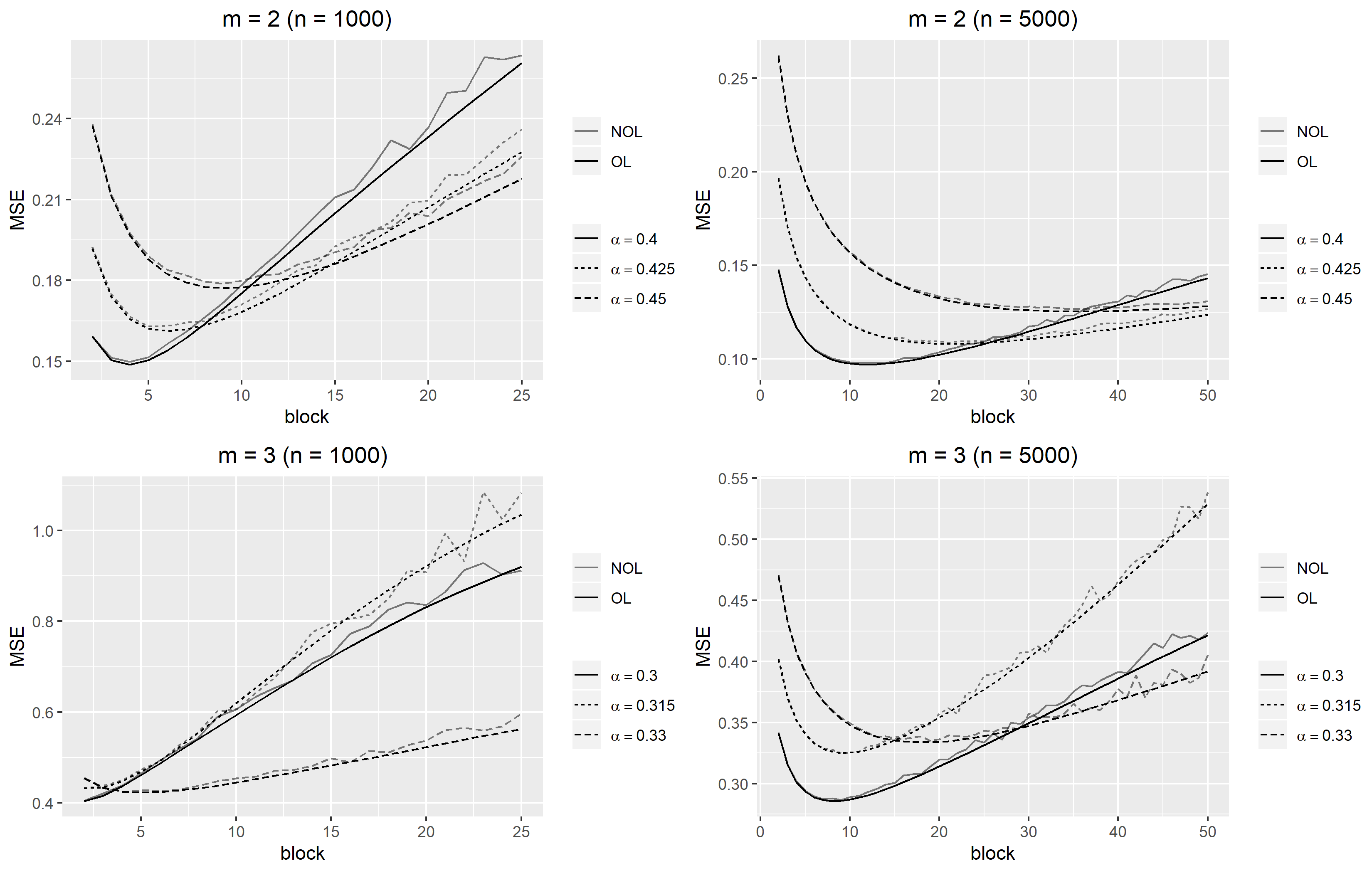
Refer to caption
Figure 1: MSE curves (over block length $\ell$) for resampling estimators with different LRD processes $(m,\alpha)$.
Table 1: Optimal OL block sizes for LRD series with Hermite ranks $m=2$ and $3$
$m=2$ $m=3$
$\alpha$ 0.400 0.425 0.450 0.300 0.315 0.330
$n=1000$ 4 6 9 2 3 5
$n=5000$ 12 21 35 8 9 18

6.2 Resampling variance estimation by empirical block size

We next examine empirical block choices for resampling variance estimation of the sample mean and provide comparison to other approaches under LRD. Application to another functional is then considered.

We use the data-based rule (12) of Section 4.3 for choosing a block size. We first compare resampling estimators $\widehat{V}_{\ell}$ of the sample mean’s variance $v_{n,{\alpha m}}$ between block selections $\ell=\widehat{\ell}_{n}$ and $\ell=\lfloor n^{1/2}\rfloor$, where the latter represents a reasonable choice under LRD by theory in Section 4.1. OL blocks are used along with local Whittle estimation $\widehat{\alpha m}$ of the memory parameter ${\alpha m}$ (Sec. 4.2). Similarly to Section 6.1, we simulated samples from LRD processes defined by $X_{t}=H_{m}(Z_{t})$ for $m=2$ with $\alpha=0.20,0.45$ or $m=3,\alpha=0.20,0.30$ and approximated the MSE $\mathrm{E}(\widehat{V}_{\ell}-v_{n,{\alpha m}})^{2}/v_{n,{\alpha m}}^{2}$ using $500$ simulations. Table 2 provides these results. Estimated blocks $\widehat{\ell}_{n}$ are generally better than the default $\lfloor n^{1/2}\rfloor$, though the latter is also competitive. The default seems preferable with a small sample size and particularly strong dependence (e.g., $n=500$, $m=3,\alpha=0.2$), but empirical block selections show improved MSEs with increased sample sizes $n=1000,2000$ under LRD.

For comparison against resampling variance estimators, we also consider the Bartlett-kernel heteroskedasticity and autocorrelation consistent (HAC) estimator [52] and the memory and autocorrelation consistent (MAC) estimator [45], whose large-sample properties have been studied for the sample mean with linear LRD processes (cf. [2, 18]), but not for transformed LRD series $X_{t}=G(Z_{t})$. As numerical suggestions from [2], we implemented HAC and MAC estimators of the sample mean’s variance using bandwidths $\lfloor n^{1/5}\rfloor$, $\lfloor n^{4/5}\rfloor$, respectively; the HAC approach further used local Whittle estimation of the memory parameter ${\alpha m}$, like the resampling estimator. The MSEs of HAC/MAC estimators are given in Table 3 (approximated from 500 simulation runs) for comparison against the resampling estimators in Table 2 with the same processes. For the process $X_{t}=H_{2}(Z_{t})$ with $\alpha=0.45$, HAC/MAC estimators emerge as slightly better than the resampling approach with estimated block sizes, though the resampling estimator outperforms HAC/MAC estimators as the dependence increases (smaller $\alpha$) or as the Hermite rank increases ($m=3$). With small sample sizes $n$ and strong dependence, the HAC estimator can exhibit large MSEs, indicating that the bandwidth $\lfloor n^{1/5}\rfloor$ is perhaps too small for the non-linear LRD series in these settings. In comparison, the empirical block selections with resampling estimators show consistently reasonable MSE-performance among all cases, which is appealing.

We further consider a different statistical functional with resampling estimators and empirical blocks $\widehat{\ell}_{n}$. In the notation of Section 5, we simulated stretches $Y_{1},\ldots,Y_{n}$ of LRD processes defined by $Y_{t}=H_{2}(Z_{t})$ or $Y_{t}=\sin(Z_{t})$ and considered an L-estimator $T_{n}$ as a 40% trimmed mean based on the empirical distribution $F_{n}$ (i.e., $\delta_{1}=1-\delta_{2}=0.2$ in Example 3, Sec. 5). For either process, the influence function $X_{t}\equiv IF(Y_{t},F)=Y_{t}I(F^{-1}(0.2)<Y_{t}<F^{-1}(0.8))/0.6$ has Hermite rank $m=1$, where $F$ and $F^{-1}$ denote the distribution and quantile functions, respectively, of $Y_{t}$. To estimate the variance, say $v_{n,{\alpha m}}$, of $n^{\alpha m/2}T_{n}$, we apply the substitution method (Sec. 5.1). That is, using estimated influences $\widehat{X}_{t}\equiv IF(Y_{n},F_{n})=Y_{t}I(F_{n}^{-1}(0.2)<Y_{t}<F_{n}^{-1}(0.8))/0.6$, we obtain an estimator $\widehat{\alpha m}$ of the memory-parameter by local Whittle estimation and compute a plug-in resampling variance estimator $\widehat{V}_{\ell}(\widehat{X})$. Table 4 provides MSEs (i.e., $\mathrm{E}(\widehat{V}_{\ell}(\widehat{X})-v_{n,{\alpha m}})^{2}/v_{n,{\alpha m}}^{2}$ approximated from 500 simulation runs) with block choices $\ell=\widehat{\ell}_{n}$ or $\lfloor n^{1/2}\rfloor$ over sample sizes $n=500,1000,2000$. The empirical block selections perform better than the default $\lfloor n^{1/2}\rfloor$ with the plug-in variance estimator here, though the choice $\lfloor n^{1/2}\rfloor$ appears also reasonable.

Table 2: MSE for resampling estimators $\widehat{V}_{\ell}$ of sample mean’s variance based on blocks $\ell=\widehat{\ell}_{n}$ or $\ell=\lfloor n^{1/2}\rfloor$ with LRD series $X_{t}\equiv G(Z_{t})$ with $G=H_{2}(Z_{t})$ $(m=2)$ and $G(Z_{t})=H_{3}(Z_{t})$ $(m=3)$.
$n=500$ $n=1000$ $n=2000$
$G/m$ $\alpha$ $\widehat{\ell}_{n}$ $\lfloor n^{1/2}\rfloor$ $\widehat{\ell}_{n}$ $\lfloor n^{1/2}\rfloor$ $\widehat{\ell}_{n}$ $\lfloor n^{1/2}\rfloor$
$m=2$ $0.20$ 0.294 0.316 0.236 0.248 0.180 0.214
$0.45$ 0.270 0.312 0.269 0.293 0.280 0.292
$m=3$ $0.20$ 0.917 0.754 0.805 0.858 0.455 0.495
$0.30$ 0.270 0.294 0.396 0.413 0.393 0.393
Table 3: MSE for HAC and MAC estimators of sample mean’s variance with LRD series $X_{t}\equiv G(Z_{t})$ with $G=H_{2}(Z_{t})$ $(m=2)$ and $G(Z_{t})=H_{3}(Z_{t})$ $(m=3)$.
$n=500$ $n=1000$ $n=2000$
$G/m$ $\alpha$ HAC MAC HAC MAC HAC MAC
$m=2$ $0.20$ 8.297 0.336 0.989 0.250 0.286 0.174
$0.45$ 0.256 0.252 0.265 0.257 0.279 0.267
$m=3$ $0.20$ 26.43 1.667 1.492 0.797 1.020 0.804
$0.30$ 0.515 0.442 0.379 0.378 0.369 0.358
Table 4: MSE for plug-in resampling estimators $\widehat{V}_{\ell}(\widehat{X})$ of the variance of the 40% trimmed mean statistic $T_{n}$ based on blocks $\ell=\widehat{\ell}_{n}$ or $\ell=\lfloor n^{1/2}\rfloor$ with LRD series $Y_{t}\equiv H_{2}(Z_{t})$ or $Y_{t}=\sin(Z_{t})$.
$n=500$ $n=1000$ $n=2000$
$Y_{t}$ $\alpha$ $\widehat{\ell}_{n}$ $\lfloor n^{1/2}\rfloor$ $\widehat{\ell}_{n}$ $\lfloor n^{1/2}\rfloor$ $\widehat{\ell}_{n}$ $\lfloor n^{1/2}\rfloor$
$H_{2}(Z_{t})$ $0.20$ 0.463 0.494 0.383 0.413 0.366 0.402
$0.45$ 0.568 0.603 0.565 0.585 0.565 0.575
$\sin(Z_{t})$ $0.20$ 0.608 0.641 0.597 0.613 0.590 0.606
$0.30$ 0.561 0.589 0.565 0.582 0.550 0.565

6.3 Resampling distribution estimation by empirical block size

Block selection also plays an important role in other resampling inference, such as approximating full sampling distributions with block bootstrap for purposes of tests and confidence intervals. While optimal block sizes for distribution estimation are difficult and unknown under LRD, we may apply blocking notions developed here for guidance. For distributional approximations of sample means and other statistics as in Section 5, the block bootstrap is valid with transformed LRD series when a normal limit exists (e.g., Hermite rank $m=1$) [29]. Such normality may occur commonly in practice [7] and can be further assessed as described in Section 6.4.

To study empirical blocks for distribution estimation with the bootstrap, we consider two LRD processes as $Y_{t}=\sin(Z_{t})$ or $Y_{t}=Z_{t}+20^{-1}H_{2}(Z_{t})$ defined by Gaussian $\{Z_{t}\}$ as before with memory exponent $\alpha$. Based on a size $n$ sample, block bootstrap is applied to approximate the distribution of $\Delta_{n}\equiv n^{\widehat{\alpha m}/2}|T_{n}-\theta|$, where $T_{n}\equiv T(F_{n})$ represents either the sample mean or the 40% trimmed mean (Example 3, Sec. 5)), while $\theta\equiv T(F)$ denotes the corresponding process mean or trimmed mean parameter. In sample mean case, we compute $\widehat{\alpha m}$ using local Whittle estimation with data stretch $X_{1}=Y_{1},\ldots,X_{n}=Y_{n}$ and define a bootstrap average $\bar{X}_{b\ell}^{*}$ by resampling $b\equiv\lfloor n/\ell\rfloor$ OL data blocks of length $\ell$ (see Sec 2.2); the bootstrap version of $\Delta_{n}$ is then $\Delta_{n}^{*}\equiv b^{1/2}\ell^{\widehat{\alpha m}/2}|\bar{X}^{*}_{b\ell}-\mathrm{E}_{*}\bar{X}^{*}_{b\ell}|$ (cf. [29]), where $\mathrm{E}_{*}\bar{X}^{*}_{b\ell}=\sum_{i=1}^{n-\ell+1}\bar{X}_{i,\ell}/(n-\ell+1)$ is a bootstrap expected average. In the trimmed mean case, the estimator $\widehat{\alpha m}$ and the bootstrap approximation $\Delta_{n}^{*}$ are similarly defined from estimated values $\widehat{X}_{t}\equiv IF(Y_{n},F_{n})=Y_{t}I(F_{n}^{-1}(0.2)<Y_{t}<F_{n}^{-1}(0.8))/0.6$, $t=1,\ldots,n$. We construct 95% bootstrap confidence intervals for $\theta$ by approximating the 95th percentile of $\Delta_{n}$ with the bootstrap counterpart from $\Delta_{n}^{*}$ (based on 200 bootstrap re-creations). Note that, for these processes and statistics, the effective Hermite rank is $m=1$ (i.e., the rank of $X_{t}=IF(Y_{t},F)$) so that the bootstrap should be valid in theory.

We used the empirical rule (12) as a guide for selecting a block length $\ell$. Table 5 shows the empirical coverages of 95% bootstrap intervals with samples of size $n=1000$ or $n=5000$ (based on 500 simulation runs). For strongest LRD $\alpha=0.02$, bootstrap intervals exhibit under-coverage, as perhaps expected, though accuracy improves with increasing sample size $n$ in this case. The bootstrap performs well in the other cases of long-memory. The coverage rates of bootstrap intervals are closer to the nominal level with empirically chosen blocks $\widehat{\ell}_{n}$ compared to a standard choice $\lfloor n^{1/2}\rfloor$, for both the sample mean and trimmed mean. This suggests that the driven-data rule for blocks provides a reasonable guidepost for resampling distribution estimation, as an application beyond variance estimation.

Table 5: Empirical coverage probabilities of 95% block bootstrap confidence intervals for the process mean or 40% trimmed mean, based on block sizes $\ell=\widehat{\ell}_{n}$ or $\ell=\lfloor n^{0.5}\rfloor$, with LRD series as $\sin(Z_{t})$ or $Z_{t}+20^{-1}H_{2}(Z_{t})$.
Mean
$\alpha=0.20$ $\alpha=0.50$ $\alpha=0.80$
$\ell$ $n=1000$ $5000$ $n=1000$ $5000$ $n=1000$ $5000$
$\sin(Z_{t})$ $\widehat{\ell}_{n}$ 0.820 0.866 0.932 0.944 0.964 0.958
$\lfloor n^{1/2}\rfloor$ 0.766 0.814 0.878 0.914 0.958 0.934
$Z_{t}+\frac{1}{20}H_{2}(Z_{t})$ $\widehat{\ell}_{n}$ 0.848 0.864 0.922 0.930 0.942 0.960
$\lfloor n^{1/2}\rfloor$ 0.806 0.854 0.914 0.894 0.938 0.952
Trimmed Mean
$\alpha=0.20$ $\alpha=0.50$ $\alpha=0.80$
$\ell$ $n=1000$ $5000$ $n=1000$ $5000$ $n=1000$ $5000$
$\sin(Z_{t})$ $\widehat{\ell}_{n}$ 0.798 0.848 0.934 0.942 0.964 0.950
$\lfloor n^{1/2}\rfloor$ 0.752 0.792 0.892 0.920 0.962 0.946
$Z_{t}+\frac{1}{20}H_{2}(Z_{t})$ $\widehat{\ell}_{n}$ 0.864 0.876 0.930 0.916 0.956 0.980
$\lfloor n^{1/2}\rfloor$ 0.828 0.852 0.918 0.908 0.876 0.754

6.4 A test of Hermite rank/normality

In a concluding numerical example, we wish to illustrate that data blocking has impacts for inference under LRD beyond the resampling. One basic application of data blocks is for testing the null hypothesis that the Hermite rank is $m=1$ for a transformed LRD process $X_{t}=G(Z_{t})$ against the alterative $m>1$. This type of assessment has practical value in application. For example, analyses in financial econometrics can involve LRD models with assumptions about $m$ (cf. [11]). More generally, inference from sample averages under LRD may use normal theory only if $m=1$ [47, 48]. Even considering resampling approximations under LRD, the block bootstrap (i.e., full data re-creation) becomes valid when $m=1$ [29], while subsampling (i.e., small scale re-creation) should be used instead if $m>1$ [6, 10, 20].

Based on data $X_{1},\ldots,X_{n}$ from a LRD process $X_{t}=G(Z_{t})$, a simple assessment of $H_{0}:m=1$ can be based on data blocks of $\ell$ as follows. The idea is to make averages (say) $W_{i}\equiv\sum_{j=1}^{\ell}X_{j+\ell(i-1)}/\ell$ of length $\ell$ blocks, $i=1,\ldots,b\equiv\lceil n/\ell\rceil$, as in Section 2.2, and then check their agreement to normality. Letting $\Phi(\cdot)$ denote a standard normal cdf, we compare the collection of residuals $R_{i}\equiv\Phi((W_{i}-\bar{W})/S_{W})$ to a uniform$(0,1)$ distribution, where $\bar{W},S_{W}$ are the average and standard deviation of $\{W_{1},\ldots,W_{b}\}$. In a usual fashion, we can assess uniformity by applying a Kolmogorov–Smirnov statistic or an Anderson-Darling [1] statistic (e.g., $A\equiv-b-b^{-1}\sum_{i=1}^{b}(2i-1)\log\{R_{(i)}[1-R_{(b+1-i)}]\}$ for ordered $R_{(i)}$). Of course, the distribution of such a test statistic requires calibration under the null $H_{0}:m=1$. However, a central limit theorem [49] for LRD processes $X_{t}=G(Z_{t})$ when $m=1$ gives

$\displaystyle\frac{1}{\sqrt{\mathrm{Var}(\bar{X}_{n})}}\frac{1}{n}\sum_{i=1}^{\lfloor nt\rfloor}\left(X_{i}-\mu\right)\overset{d}{\to}cB_{H}(t),\quad 0\leq t\leq 1,$ (14)

as $n\to\infty$, where $B_{H}(t)$ denotes fractional Brownian motion with Hurst index $H=1-\alpha/2\in(0,1)$ and $c>0$ is a process constant. Note that (14) no longer holds under LRD when $m>1$, which aids in testing. The property (14) suggests a simple bootstrap procedure for re-creating the null distribution of residual-based test statistics, given in Algorithm 1, because such statistics are invariant to the location-scale used in a bootstrap sample.

Data: Given a LRD sample $X_{1},..,X_{n}$.
Set initializations: block size $\ell$; number $M$ of resamples; and significance level $\alpha_{\mathrm{sig}}=0.05$.
Step 1. Calculate a test statistic $T_{0}$ for normality (e.g., Anderson-Darling) from block averages;
Step 2. Estimate $\widehat{\alpha m}$ the memory parameter $\alpha m$ or Hurst Index $\widehat{H}=1-\widehat{\alpha m}/2$;
Step 3. for $k=1,\ldots,M$ do
       (i) Simulate a Fractional Brownian motion sample $\{B^{*}_{\scriptscriptstyle\widehat{H}}(\frac{1}{n}),\ldots,B^{*}_{\scriptscriptstyle\widehat{H}}(\frac{n}{n})$} with Hurst index $\widehat{H}$;
      
      (ii) Obtain a bootstrap sample $X_{1}^{*},\ldots,X_{n}^{*}$ as $X_{1}^{*}=B^{*}_{\scriptscriptstyle\widehat{H}}(\frac{1}{n})$ and $X_{j}^{*}=B^{*}_{\scriptscriptstyle\widehat{H}}(\frac{j}{n})-B^{*}_{\scriptscriptstyle\widehat{H}}(\frac{j-1}{n})$, $j=2,\ldots,n$;
      
      (iii) Calculate the $k$th bootstrap test statistic, $T^{*}_{k}$, for normality from block averages in $X_{1}^{*},\ldots,X_{n}^{*}$;
      
end for
Step 4. Compute $\widehat{q}$ as the $1-\alpha_{\mathrm{sig}}$ sample percentile of $\{T^{*}_{1},\ldots,T^{*}_{M}\}$;
Step 5. Reject if $T_{0}>\widehat{q}$.
Algorithm 1 Hermite rank test for $m=1$ (normality) from LRD series

The role of data blocking for tests of Hermite rank $H_{0}:m=1$ with LRD series $X_{t}=G(Z_{t})$ may be traced to recent work of [9]. Those authors test for $m=1$ (normality) with a cumulant-based two-sample $t$-test, using two samples generated from data by different OL block resampling approaches. Our block-based test is different and perhaps more basic. To briefly compare these tests, we use data generation settings from [9] where $X_{t}=G(Z_{t})$ with $G(z)=z+20^{-1}H_{2}(z)+(20\sqrt{3})^{-1}H_{3}(z)$ (i.e., $m=1$) or $G(z)=\cos(z)$ (i.e., $m=2$), and $Z_{t}$ denotes a standardized FAIRMA$(0,(1-\alpha)/2,0)$ Gaussian process for $\alpha=0.2,0.8$. The test in [9] uses block lengths $\ell=n^{1/4}$ or $\ell=n^{1/2}$, where some best-case results provided there assume the memory parameter to be known. To facilitate comparison against these, we simply use a similar block $\ell=n^{1/2}$ for our test, as a reasonable choice under LRD, and consider both OL/NOL blocks; we also use local Whittle estimation of the memory parameter along with 200 resamples in Algorithm 1. Table 6 lists power (based on 500 simulation runs) of our test using a 5% nominal level compared to test findings of [9] (Table 2); we report an Anderson-Darling statistic in Table 6 though a Kolmogorov–Smirnov statistic produced similar results. Both the proposed test and the [9]-test maintain the nominal size for the LRD processes with $m=1$, but our block-based test has much larger power for the LRD process defined by $m=2$ and $\alpha=0.2$. The process defined by $m=2$ and $\alpha=0.8$ in Table 6 is actually SRD; as both our test and the [9]-test are block-based assessments of normality, both tests should maintain their sizes in this case and our test performs a bit better. This illustrates that data-blocking has potential for assessments beyond usage in resampling.

Table 6: Rejection rates of nominal 5% tests of Hermite rank $m=1$ from block-based statistic (Algorithm 1 with OL/NOL blocks $\ell=\lfloor n^{1/2}\rfloor$) with LRD series $X_{t}\equiv G(Z_{t})$ using $G_{1}(z)=z+20^{-1}H_{2}(z)+(20\sqrt{3})^{-1}H_{3}(z)$ or $G_{2}(z)=\cos(z)$. Results from the test of [9] (OL blocks $\ell=n^{1/2}$ or $n^{1/4}$) are included.
$\alpha=0.20$ $\alpha=0.80$
$G/m$ Testing Method $n=400$ $1000$ $10000$ $n=400$ 1000 10000
$G_{1}$, $m=1$ Algorithm 1 OL 0.06 0.06 0.07 0.05 0.08 0.07
NOL 0.10 0.06 0.08 0.06 0.05 0.06
[9]-test $\ell=n^{1/2}$ 0.04 0.05 0.03 0.01 0.03 0.03
$\ell=n^{1/4}$ 0.03 0.04 0.04 0.07 0.06 0.03
$G_{2}$, $m=2$ Algorithm 1 OL 0.60 0.85 0.99 0.13 0.14 0.13
NOL 0.45 0.68 0.99 0.06 0.09 0.07
[9]-test $\ell=n^{1/2}$ 0.11 0.23 0.26 0.13 0.13 0.20
$\ell=n^{1/4}$ 0.19 0.24 0.32 0.24 0.16 0.27

7 Concluding Remarks

While block-based resampling methods provide useful estimation under data dependence, their performance is intricately linked to a block length parameter, which is important to understand. This problem has been extensively investigated under weak or short-range dependence (SRD) (cf. [31], ch. 3), though relatively little has been known for long-range dependence (LRD), especially outside the pure Gaussian case (cf. [26]). For general long-range dependent (LRD) $X_{t}=G(Z_{t})$ processes, based on transforming a LRD Gaussian series $Z_{t}$, results here showed that properties and best block sizes with resampling variance estimators under LRD can intricately depend on covariance strength and the structure of non-linearity in $G(\cdot)$. The long-memory guess $O(n^{1/2})$ for block size [22] may have optimal order at times, owing more to such non-linearity rather than intuition about LRD. Additionally, we provided a data-based rule for best block selection, which was shown to be consistent under complex cases for blocks with LRD. While we focused on a variance estimation problem with resampling under LRD, block selection for distribution estimation is also of interest, though seemingly requires further difficult study of distributional expansions for statistics from LRD series $X_{t}=G(Z_{t})$. However, we showed that the block selections developed here can provide helpful benchmarks for choosing block size with resampling or other block-based inference problems under LRD.

The current work may also suggest future possibilities toward estimating the Hermite $m$ rank (or other ranks) under LRD. No estimators of $m$ currently exist; instead, only estimation of the long-memory exponent ${\alpha m}$ of $X_{t}=G(Z_{t})$ has been possible, which depends on the covariance decay rate $\alpha<1/m$ of $Z_{t}$. Results here established that the variance of a block resampling estimator depends only on $\alpha$, apart from the Hermite rank $m$ itself. This suggests that some higher-order moment estimation may be investigated for separately estimating the memory coefficient $\alpha$ and Hermite rank $m$ under LRD.

Appendix A Coefficient of Optimal Block Size

The coefficient $K_{\alpha,m,m_{2}}$ of Corollary 4.1 is presented in cases with notation: $A\equiv\mathcal{B}_{0}^{2}(m)$, $B\equiv(2C_{0}^{m_{2}}J_{m_{2}}^{2}/m_{2}!)^{2}$, $C\equiv(\mathcal{B}_{0}(m)+2\sum_{j=m_{2}}^{\infty}\sum_{k=1}^{\infty}[\gamma_{Z}(k)]^{j}J^{2}_{j}/j!)^{2}$, and $D\equiv(2C_{0}^{m_{2}}/[(1-m_{2}\alpha)(2-m_{2}\alpha)](J_{m_{2}}^{2}/m_{2}!))^{2}$ related to (7); $E\equiv v^{2}_{\infty,\alpha m}$ in (4); and $F\equiv a_{\alpha}$ from Theorem 3.2.

Case $1$: $m_{2}=\infty$

$$K_{\alpha,m,m_{2}}=\left\{\begin{array}[]{ll}\frac{-(1-2\alpha)\sqrt{AE}+\sqrt{(1-2\alpha)^{2}{AE}+4\alpha(1-\alpha)A(E+F)}}{2\alpha(E+F)}&\text{ if }0<\alpha<0.5,m=1\\ \left(\frac{A}{F}\right)^{0.5}&\text{ if }\alpha=0.5,m=1\\ \left(\frac{2A(1-\alpha)}{F}\right)^{\frac{1}{3-2\alpha}}&\text{ if }0.5<\alpha<1,m=1\\ \left(\frac{A(1-\alpha m)}{F\alpha}\right)^{\frac{1}{2(1+\alpha-\alpha m)}}&\text{ if }0<\alpha<\frac{1}{m},m\geq 2\end{array}\right.$$

Case $2$: $m_{2}<\infty$ with $\alpha m_{2}>1$

$$K_{\alpha,m,m_{2}}=\left\{\begin{array}[]{ll}\frac{-(1-2\alpha)\sqrt{CE}+\sqrt{(1-2\alpha)^{2}CE+4\alpha(1-\alpha)C(E+F)}}{2\alpha(E+F)}&\text{ if }\frac{1}{m_{2}}<\alpha<0.5,m=1\\ \left(\frac{C}{F}\right)^{0.5}&\text{ if }\alpha=0.5,m=1\\ \left(\frac{2C(1-\alpha)}{F}\right)^{\frac{1}{3-2\alpha}}&\text{ if }\max\{\frac{1}{m_{2}},0.5\}<\alpha<1,m=1\\ \left(\frac{C(1-\alpha m)}{F\alpha}\right)^{\frac{1}{2(1+\alpha-\alpha m)}}&\text{ if }\frac{1}{m_{2}}<\alpha<\frac{1}{m},m\geq 2\end{array}\right.$$

Case $3$: $m_{2}<\infty$ with $\alpha m_{2}=1$

$$K_{\alpha,m,m_{2}}=\left\{\begin{array}[]{ll}\frac{-(1-2\alpha)\sqrt{BE}+\sqrt{(1-2\alpha)^{2}BE+4\alpha(1-\alpha)B(E+F)}}{2\alpha(E+F)}&\text{ if }0<\alpha=\frac{1}{m_{2}}<0.5,m=1\\ \left(\frac{B}{F}\right)^{0.5}&\text{ if }\alpha=\frac{1}{m_{2}}=0.5,m=1\\ \left(\frac{B(1-\alpha m)}{F\alpha}\right)^{\frac{1}{2(1+\alpha-\alpha m)}}&\text{ if }0<\alpha=\frac{1}{m_{2}}<0.5,m\geq 2\end{array}\right.$$

Case $4$: $m_{2}<\infty$ with $\alpha m_{2}<1$

$$K_{\alpha,m,m_{2}}=\left\{\begin{array}[]{ll}\left(\frac{(m_{2}-2)+\sqrt{(m_{2}-2)^{2}+(m_{2}-1)(E+F)D}}{E+F}\right)^{\frac{1}{\alpha m_{2}}}&\text{ if }0<\alpha<\frac{1}{m_{2}},m=1\\ \left(\frac{D(m_{2}-m)}{F}\right)^{\frac{1}{2\alpha(1+m_{2}-m)}}&\text{ if }0<\alpha<\frac{1}{m_{2}},m\geq 2\\ \end{array}\right.$$

Appendix B Proof of Theorem 3.2

The appendix considers the proof for the large-sample variance (Theorem 3.2) of resampling estimators. Proofs are other results are shown in the supplement [54]. To derive variance expansions of Theorem 3.2, we first consider the OL block variance estimator $\widehat{V}_{\ell,{\alpha m},{\scriptscriptstyle OL}}=\sum_{i=1}^{N}\ell^{\alpha m}(\bar{X}_{i,\ell}-\mu)^{2}/N-\ell^{\alpha m}(\widehat{\mu}_{n,{\scriptscriptstyle OL}}-\mu)^{2}$ from (5), expressed in terms of the process mean $\mathrm{E}X_{t}=\mu$, the number $N=n-\ell+1$ of blocks, the block averages $\bar{X}_{i,\ell}\equiv\sum_{j=i}^{i+\ell-1}X_{j}/\ell$ (integer $i$), and $\widehat{\mu}_{n,{\scriptscriptstyle OL}}=\sum_{i=1}^{N}\bar{X}_{i,\ell}/N$. Due to mean centering, we may assume $\mu=0$ without loss of generality. We then write the variance of $\widehat{V}_{\ell,{\alpha m},{\scriptscriptstyle OL}}$ as

$$\mathrm{Var}\left(\widehat{V}_{\ell,{\alpha m},{\scriptscriptstyle OL}}\right)=v_{1,\ell}+v_{2,\ell}-2c_{\ell},\qquad c_{\ell}\equiv\mathrm{Cov}\left(\frac{1}{N}\sum_{i=1}^{N}\ell^{\alpha m}\bar{X}_{i,\ell}^{2},\ell^{\alpha m}\widehat{\mu}_{n,{\scriptscriptstyle OL}}^{2}\right)=c_{a,\ell}+c_{b,\ell},$$
$\displaystyle v_{1,\ell}\equiv\mathrm{Var}\left(\frac{1}{N}\sum_{i=1}^{N}\ell^{\alpha m}\bar{X}_{i,\ell}^{2}\right)=v_{1a,\ell}+v_{1b,\ell},\qquad v_{2,\ell}\equiv\mathrm{Var}\left(\ell^{\alpha m}\widehat{\mu}_{n,{\scriptscriptstyle OL}}^{2}\right)=v_{2a,\ell}+v_{2b,\ell},$

where each variance/covariance component $v_{1,\ell}$, $v_{2,\ell}$ and $c_{\ell}$ is decomposed into two further subcomponents

$\displaystyle v_{1a,\ell}$ $\displaystyle\equiv$ $\displaystyle 2\frac{\ell^{2{\alpha m}}}{N}\sum_{k=-N}^{N}\left(1-\frac{|k|}{N}\right)\left[\mathrm{Cov}(\bar{X}_{0,\ell},\bar{X}_{k,\ell})\right]^{2},$
$\displaystyle v_{1b,\ell}$ $\displaystyle\equiv$ $\displaystyle\frac{\ell^{2{\alpha m}}}{N}\sum_{k=-N}^{N}\left(1-\frac{|k|}{N}\right)\mathrm{cum}(\bar{X}_{0,\ell},\bar{X}_{0,\ell},\bar{X}_{k,\ell},\bar{X}_{k,\ell}),$ (15)
$\displaystyle v_{2a,\ell}$ $\displaystyle\equiv$ $\displaystyle 2\ell^{2{\alpha m}}\left[\mathrm{Var}(\widehat{\mu}_{n,{\scriptscriptstyle OL}})\right]^{2},$
$\displaystyle v_{2b,\ell}$ $\displaystyle\equiv$ $\displaystyle\ell^{2{\alpha m}}\mathrm{cum}(\widehat{\mu}_{n,{\scriptscriptstyle OL}},\widehat{\mu}_{n,{\scriptscriptstyle OL}},\widehat{\mu}_{n,{\scriptscriptstyle OL}},\widehat{\mu}_{n,{\scriptscriptstyle OL}}),$
$\displaystyle c_{a,\ell}$ $\displaystyle\equiv$ $\displaystyle 2\frac{\ell^{2{\alpha m}}}{N}\sum_{i=1}^{N}\left[\mathrm{Cov}(\bar{X}_{i,\ell},\widehat{\mu}_{n,{\scriptscriptstyle OL}})\right]^{2},$
$\displaystyle c_{b,\ell}$ $\displaystyle\equiv$ $\displaystyle\frac{\ell^{2{\alpha m}}}{N^{3}}\sum_{i=1}^{N}\sum_{j=1}^{N}\sum_{k=1}^{N}\mathrm{cum}(\bar{X}_{i,\ell},\bar{X}_{i,\ell},\bar{X}_{j,\ell},\bar{X}_{k,\ell}),$

consisting of sums involving 4th order cumulants ($v_{1b,\ell},v_{2b,\ell},c_{b,\ell}$) or sums involving covariances ($v_{1a,\ell},v_{2a,\ell},c_{a,\ell}$). The second decomposition step follows from the product theorem for cumulants (e.g., $\mathrm{Cov}(Y_{1}Y_{2},Y_{3}Y_{4})=\mathrm{Cov}(Y_{1},Y_{3})\mathrm{Cov}(Y_{2},Y_{4})+\mathrm{Cov}(Y_{1},Y_{4})\mathrm{Cov}(Y_{2},Y_{3})+\mathrm{cum}(Y_{1},Y_{2},Y_{3},Y_{4})$ for arbitrary random variables with $\mathrm{E}Y_{i}=0$ and $\mathrm{E}Y_{i}^{4}<\infty$). Note that $\mathrm{E}X_{t}^{4}=\mathrm{E}[G(Z_{0})]^{4}<\infty$ and $G\in\overline{\mathcal{G}}_{4}(1)$ imply these variance components exist finitely for any $n,\ell$ (see (S.9) or Lemma 3 of the supplement  [54]). Collecting terms, we have

$$\mathrm{Var}\left(\widehat{V}_{\ell,{\alpha m},{\scriptscriptstyle OL}}\right)=\Gamma_{\ell,{\scriptscriptstyle OL}}+\Delta_{\ell,{\scriptscriptstyle OL}}$$

where $\Gamma_{\ell,{\scriptscriptstyle OL}}\equiv v_{1a,\ell}+v_{2a,\ell}-2c_{a,\ell}$ and $\Delta_{\ell,{\scriptscriptstyle OL}}\equiv v_{1b,\ell}+v_{2b,\ell}-2c_{b,\ell}$ denote sums over covariance-terms $\Gamma_{\ell,{\scriptscriptstyle OL}}$ or sums of 4th order cumulant terms $\Delta_{\ell,{\scriptscriptstyle OL}}$. In the NOL estimator case $\widehat{V}_{\ell,{\alpha m},\scriptscriptstyle NOL}$, the variance expansion is similar $\mathrm{Var}\left(\widehat{V}_{\ell,{\alpha m},\scriptscriptstyle NOL}\right)=\Gamma_{\ell,\scriptscriptstyle NOL}+\Delta_{\ell,\scriptscriptstyle NOL}$ with the convention that $\Gamma_{\ell,\scriptscriptstyle NOL},\Delta_{\ell,\scriptscriptstyle NOL}$ are defined by replacing the OL block number $N=n-\ell+1$, averages $\bar{X}_{i,\ell}$ (or $\bar{X}_{j,\ell},\bar{X}_{k,\ell}$) and estimator $\widehat{\mu}_{n,{\scriptscriptstyle OL}}=\sum_{i=1}^{N}\bar{X}_{i,\ell}/N$ with the NOL counterparts $b=\lfloor n/\ell\rfloor$, $\bar{X}_{1+(i-1)\ell,\ell}$ (or $\bar{X}_{1+(j-1)\ell,\ell},\bar{X}_{1+(k-1)\ell,\ell}$) and $\widehat{\mu}_{n,\scriptscriptstyle NOL}=\sum_{i=1}^{b}\bar{X}_{1+(i-1)\ell,\ell}/b$ in $v_{1a,\ell},v_{2a,\ell},c_{a,\ell},v_{1b,\ell},v_{2b,\ell},c_{b,\ell}$.

Let $\Gamma_{\ell}$ denote either counterpart $\Gamma_{\ell,{\scriptscriptstyle OL}}$ or $\Gamma_{\ell,\scriptscriptstyle NOL}$, and $\Delta_{\ell}$ denote either $\Delta_{\ell,{\scriptscriptstyle OL}}$ or $\Delta_{\ell,\scriptscriptstyle NOL}$. Theorem 3.2 then follows by establishing that

$$\Gamma_{\ell}=\left\{\begin{array}[]{lcl}O\left(\left(\frac{\ell}{n}\right)^{\min\{1,2{\alpha m}\}}[\log n]^{I(2{\alpha m}=1)}\right)=o\left(\left(\frac{\ell}{n}\right)^{2\alpha}\right)&&\mbox{if $m\geq 2$}\\[2.84544pt] a_{\alpha}\left(\frac{\ell}{n}\right)^{\min\{1,2\alpha\}}[\log n]^{I(\alpha=1/2)}\big{(}1+o(1)\big{)}&&\mbox{if $m=1$},\end{array}\right.$$

and

$$\Delta_{\ell}-r_{n,\alpha,m,m_{p}}=\left\{\begin{array}[]{lcl}\phi_{\alpha,m}\left(\frac{\ell}{n}\right)^{2\alpha}\big{(}1+o(1)\big{)}&&\mbox{if $m\geq 2$}\\[5.69046pt] o\left(\left(\frac{\ell}{n}\right)^{\min\{1,2\alpha\}}[\log n]^{I(\alpha=1/2)}\right)&&\mbox{if $m=1$},\end{array}\right.$$

where $I(\cdot)$ denotes an indicator function and $r_{n,\alpha,m,m_{p}}$ is defined in Theorem 3.2. For reference, when the Hermite rank $m\geq 2$, the contribution of $\Delta_{\ell}\propto(\ell/n)^{2\alpha}$ dominates the variance of $\widehat{V}_{\ell,{\alpha m},{\scriptscriptstyle OL}}$ or $\widehat{V}_{\ell,{\alpha m},\scriptscriptstyle NOL}$; when $m=1$, the contribution of $\Gamma_{\ell}\propto(\ell/n)^{\min\{1,2\alpha\}}[\log n]^{I(\alpha=1/2)}$ instead dominates the variance in Theorem 3.2.

To establish these expansions of $\Gamma_{\ell},\Delta_{\ell}$, we require a series of technical lemmas (Lemmas 1-4), involving certain graph-theoretic moment expansions. To provide some illustration, Lemma 1 and its proof are outlined in Appendix C; the remaining lemmas are described in the supplement [54]. Define an order constant $\tau_{\ell,m}\equiv(\ell/n)^{2\alpha}$ if $m\geq 2$ and $\tau_{\ell,m}\equiv(\ell/n)^{\min\{1,2\alpha\}}[\log n]^{I(\alpha=1/2)}$ if $m=1$; we suppress the dependence of $\tau_{\ell,m}$ on $n$ and $\alpha$ for simplicity. Then, the above expansion of $\Gamma_{\ell}$ follows directly from Lemma 4 (i.e., $\Gamma_{\ell}=a_{\alpha}\tau_{\ell,1}(1+o(1))$ if $m=1$ and $\Gamma_{\ell}=o(\tau_{\ell,m})$ if $m\geq 2$). For handling $\Delta_{\ell}$, Lemma 1 gives that $v_{1b,\ell}=r_{n,\alpha,m,m_{p}}+\phi_{\alpha,m}\tau_{\ell,m}\big{(}1+o(1)\big{)}$ when $m\geq 2$ and $v_{1b,\ell}=r_{n,\alpha,m,m_{p}}+o(\tau_{\ell,m})$ when $m=1$. Combined with this, the expansion of $\Delta_{\ell}$ then follows from Lemmas 2 and 3, which respectively show that $c_{b,\ell}=o(\tau_{\ell,m})$ and $v_{2b,\ell}=o(\tau_{\ell,m})$ for any $m\geq 1$. $\Box$

Appendix C Lemma 1 (dominant 4th order cumulant terms)

In the proof of Theorem 3.2 (Appendix B), recall $v_{1b,\ell}$ from (15) represents a sum of 4th order cumulants block averages with OL blocks, where the version with NOL blocks is $v_{1b,\ell}\equiv b^{-1}\ell^{2{\alpha m}}\sum_{k=-b}^{b}\left(1-\frac{|k|}{b}\right)\mathrm{cum}(\bar{X}_{0,\ell},\bar{X}_{0,\ell},\bar{X}_{k\ell,\ell},\bar{X}_{k\ell,\ell})$. Lemma 1 provides an expansion of $v_{1b,\ell}$ under LRD, which is valid in either OL/NOL block case.

Lemma 1.

Suppose the assumptions of Theorem 3.2 ($G$ has Hermite rank $m\geq 1$ and Hermite pair-rank $m\leq m_{p}\leq\infty$) with positive constants $\phi_{\alpha,m},\lambda_{\alpha,m_{p}}$ there. Then,

$$v_{1b,\ell}=r_{n,\alpha,m,m_{p}}+\left\{\begin{array}[]{lcl}\phi_{\alpha,m}\left(\frac{\ell}{n}\right)^{2\alpha}\big{(}1+o(1)\big{)}&&\mbox{if $m\geq 2$}\\[5.69046pt] o\left(\left(\frac{\ell}{n}\right)^{\min\{1,2\alpha\}}[\log n]^{I(\alpha=1/2)}\right)&&\mbox{if $m=1$},\end{array}\right.$$

where $I(\cdot)$ denotes an indicator function and $r_{n,\alpha,m,m_{p}}$ is from Theorem 3.2.

Remark 2: The proof of Lemma 1 involves a standard, but technical, graph-theoretic representation of the 4th order cumulant among Hermite polynomials $H_{k_{1}}(Y_{1}),H_{k_{2}}(Y_{2}),H_{k_{3}}(Y_{3})$, $H_{k_{4}}(Y_{4})$ ($k_{1},k_{2},k_{3},k_{4}\geq 1$) at a generic sequence $(Y_{1},Y_{2},Y_{3},Y_{4})$ of marginally standard normal variables, with covariances $\mathrm{E}Y_{i}Y_{j}=r_{ij}=r_{ji}$ for $1\leq i<j\leq 4$. Namely, it holds that

$$\mathrm{cum}[H_{k_{1}}(Y_{1}),H_{k_{2}}(Y_{2}),H_{k_{3}}(Y_{3}),H_{k_{4}}(Y_{4})]=k_{1}!k_{2}!k_{3}!k_{4}!\sum_{A\in\mathcal{A}_{c}(k_{1},k_{2},k_{3},k_{4})}g(A)r(A),$$ (16)

where above $\mathcal{A}_{c}(k_{1},k_{2},k_{3},k_{4})$ denotes the collection of all path-connected multigraphs from a generic set of four points/vertices $p_{1},p_{2},p_{3},p_{4}$, such that point $p_{i}$ has degree $k_{i}$ for $i=1,2,3,4$. Each multigraph $A\equiv(v_{12},v_{13},v_{14},v_{23},v_{24},v_{34})\in\mathcal{A}_{c}(k_{1},k_{2},k_{3},k_{4})$ is defined by distinct counts $v_{ij}=v_{ji}\geq 0$, interpreted as the number of graph lines connecting points $p_{i}$ and $p_{j}$, $1\leq i<j\leq 4$; no other lines are possible in $A$. Then $g(A)\equiv 1/[\prod_{1\leq i<j\leq 4}(v_{ij}!)]$ represents a so-called multiplicity factor, while $r(A)\equiv\prod_{1\leq i<j\leq 4}r_{ij}^{v_{ij}}$ represents a weighted product of covariances among variables in $(Y_{1},Y_{2},Y_{3},Y_{4})$ (cf.[48]). Membership $A\in\mathcal{A}_{c}(k_{1},k_{2},k_{3},k_{4})$ requires degrees $k_{i}=\sum_{j:j\neq i}v_{ij}$ for $i=1,2,3,4$ (e.g., $k_{2}=v_{12}+v_{23}+v_{24}$) as well as a path-connection in $A$ between any two points $p_{i}$ and $p_{j}$; namely, for any given $1\leq i<j\leq 4$, an index sequence $i\equiv i_{0},i_{1},\ldots,i_{m}\equiv j\in\{1,2,3,4\}$ (for some $1\leq m\leq 3$) must exist whereby $v_{i_{u-1}i_{u}}>0$ holds for each $u=1,\ldots,m$, entailing that consecutive points among $p_{i}=p_{i_{0}},p_{i_{1}},\ldots,p_{i_{m}}=p_{j}$ are connected with lines in $A$. In (16), $\mathrm{cum}[H_{k_{1}}(Y_{1}),H_{k_{2}}(Y_{2}),H_{k_{3}}(Y_{3}),H_{k_{4}}(Y_{4})]=0$ holds whenever $\mathcal{A}_{c}(k_{1},k_{2},k_{3},k_{4})$ is empty; given integers $k_{1},k_{2},k_{3},k_{4}\geq 1$, $\mathcal{A}_{c}(k_{1},k_{2},k_{3},k_{4})$ will be empty if $k_{1}+k_{2}+k_{3}+k_{4}=2q$ fails to hold for some integer $q\geq 2$ with $\max_{i=1,2,3,4}k_{i}\leq q$. See the supplement [54] for more background and details on this graph-theoretic representation.

Proof of Lemma 1. We focus on the OL block version (15) of $v_{1b,\ell}$; the NOL block case follows by the same essential arguments, though the cumulant sums involved with NOL blocks are less involved and simpler to handle. We assume $\mu=0$ for reference; the mean $\mu\equiv\mathrm{E}G(Z_{t})$ does not impact the 4th order cumulants here. Define $\tau_{\ell,m}\equiv(\ell/n)^{2\alpha}$ if $m\geq 2$ (i.e., $\alpha<1/2$) and $\tau_{\ell,m}\equiv(\ell/n)^{\min\{1,2\alpha\}}[\log n]^{I(\alpha=1/2)}$ if $m=1$ to describe the order of interest in Lemma 1 along cases $m\geq 2$ or $m=1$.

Using Lemma 3 (i.e., $\max_{0\leq k\leq 2\ell}|\mathrm{cum}(\bar{X}_{0,\ell},\bar{X}_{0,\ell},\bar{X}_{k,\ell},\bar{X}_{k,\ell})|$ is $O(\ell^{-2{\alpha m}}))$ for $m\geq 2$ or $O(\ell^{-\alpha-\min\{1,2\alpha\}}[\log\ell]^{I(\alpha=1/2)})$ for $m=1$), we may truncate the sum $v_{1b,\ell}$ in (15) as

$\displaystyle v_{1b,\ell}=v_{1b,\ell}^{trun}+O\left(\frac{\ell^{1+I(m=1)(\alpha-\min\{1,2\alpha\})}}{n}[\log\ell]^{I(\alpha=1/2)}\right),$ (17)

where the order term is $o(\tau_{\ell,m})$. Then, using that $G\in\overline{\mathcal{G}}_{4}(1)$ (cf. (S.9) of the supplement [54]) along with the 4th order cumulant form (16) for Hermite polynomials, we may use the multi-linearity of cumulants and the Hermite expansion (2) to express $v_{1b,\ell}^{trun}$ in (17) as

$\displaystyle 2\frac{\ell^{2{\alpha m}}}{N}\sum_{k=2\ell+1}^{N}\left(1-\frac{k}{N}\right)\mathrm{cum}(\bar{X}_{0,\ell},\bar{X}_{0,\ell},\bar{X}_{k,\ell},\bar{X}_{k,\ell})\;\equiv\;v_{1b,\ell}^{trun}$ (18)
$\displaystyle=$ $\displaystyle 2\frac{\ell^{2{\alpha m}}}{N}\sum_{k=2\ell+1}^{N}\left(1-\frac{k}{N}\right)\sum_{m\leq k_{1},k_{2},k_{3},k_{4}}\left(\prod_{i=1}^{4}\frac{J_{k_{i}}}{k_{i}!}\right)\frac{1}{\ell^{4}}\times$
$\displaystyle\qquad\sum_{1\leq i_{1},i_{2},i_{3},i_{4}\leq\ell}\mathrm{cum}(H_{k_{1}}(Z_{i_{1}}),H_{k_{2}}(Z_{i_{2}}),H_{k_{3}}(Z_{i_{3}+k}),H_{k_{4}}(Z_{i_{4}+k}))$
$\displaystyle=$ $\displaystyle 2\sum_{q=2m}^{\infty}\sum_{k_{1}+k_{2}+k_{3}+k_{4}=2q,\atop m\leq k_{1},k_{2},k_{3},k_{4}\leq q}\left(\prod_{i=1}^{4}J_{k_{i}}\right)\sum_{A\in\mathcal{A}_{c}(k_{1},k_{2},k_{3},k_{4}),\atop\mathcal{A}_{c}(k_{1},k_{2},k_{3},k_{4})\neq\emptyset}g(A)\frac{1}{N}\sum_{k=2\ell+1}^{N}\left(1-\frac{k}{N}\right)R_{\ell,k}(A)$
$\displaystyle\equiv$ $\displaystyle t_{1,\ell}+t_{2,\ell}+t_{3,\ell}\mbox{\quad(say)},$

with $g(A)=1/[\prod_{1\leq i<j\leq 4}(v_{ij}!)]$, $A\equiv(v_{12},v_{13},v_{14},v_{23},v_{24},v_{34})\in\mathcal{A}_{c}(k_{1},k_{2},k_{3},k_{4})$, and

$\displaystyle\qquad R_{\ell,k}(A)$ $\displaystyle\equiv$ $\displaystyle\frac{\ell^{2{\alpha m}}}{\ell^{4}}\sum_{i_{1}=1}^{\ell}\sum_{i_{2}=1}^{\ell}\sum_{i_{3}=1}^{\ell}\sum_{i_{4}=1}^{\ell}[\gamma_{Z}(i_{1}-i_{2})]^{v_{12}}[\gamma_{Z}(i_{1}-i_{3}-k)]^{v_{13}}\times$
$\displaystyle[\gamma_{Z}(i_{1}-i_{4}-k)]^{v_{14}}[\gamma_{Z}(i_{2}-i_{3}-k)]^{v_{23}}[\gamma_{Z}(i_{2}-i_{4}-k)]^{v_{24}}[\gamma_{Z}(i_{3}-i_{4})]^{v_{34}}$

in terms of Gaussian process covariances $\gamma_{Z}(\cdot)$ from (1). In (18), we use that the Hermite rank of $G$ is $m$ (so $J_{k}=0$ for $k<m$); that the 4th order cumulants (16) of Hermite polynomials are zero when a collection $\mathcal{A}_{c}(k_{1},k_{2},k_{3},k_{4})$ is empty; and, relatedly, for given integers $k_{1},k_{2},k_{3},k_{4}\geq m$, a non-empty collection $\mathcal{A}_{c}(k_{1},k_{2},k_{3},k_{4})$ requires the number of lines, say $q\equiv(k_{1}+k_{2}+k_{3}+k_{4})/2$, of a graph $A$ in $\mathcal{A}_{c}(k_{1},k_{2},k_{3},k_{4})$ to be an integer $q\geq 2m$ with $m\leq\max_{i=1,2,3,4}k_{i}\leq q$. The three components $t_{1,\ell},t_{2,\ell}$ and $t_{3,\ell}$ in (18) are defined by splitting the sum into three mutually exclusive cases, depending on the number of lines $q\equiv(k_{1}+k_{2}+k_{3}+k_{4})/2=\sum_{1\leq i<j\leq 4}v_{ij}$ and the value of $v_{13}+v_{14}+v_{23}+v_{24}=q-v_{12}-v_{34}$ for a multigraph $A\equiv(v_{12},v_{13},v_{14},v_{23},v_{24},v_{34})\in\mathcal{A}_{c}(k_{1},k_{2},k_{3},k_{4})\neq\emptyset$; note that counts $v_{13},v_{14},v_{23},v_{24}$ involve covariances $\gamma_{Z}(\cdot)$ at large lags in (C) (i.e., larger than $\ell$ by $2k\geq\ell+1$), which is not true of counts $v_{12},v_{34}$. The three cases for defining $t_{1,\ell},t_{2,\ell}$ and $t_{3,\ell}$ are given by: (i) the case $q=2m$ with $k_{1}=k_{2}=k_{3}=k_{4}=m$, which yields

$$t_{1,\ell}\equiv 2J_{m}^{4}\sum_{A\in\mathcal{A}_{c}(m,m,m,m)\neq\emptyset}g(A)\frac{1}{N}\sum_{k=2\ell+1}^{N}\left(1-\frac{k}{N}\right)R_{\ell,k}(A);$$ (20)
$p_{1}$ $p_{2}$ $p_{3}$ $p_{4}$ $1$ $1$ $1$ $1$
Figure 2: An example of multigraph $A\equiv(1,0,1,1,0,1)\in\mathcal{A}_{c}(m,m,m,m)$ for $m=2$.

(ii) the case that $q\geq 2m+1$ where the sum over $A\in\mathcal{A}_{c}(k_{1},k_{2},k_{3},k_{4})$ is also restricted to multigraphs $A\equiv(v_{12},v_{13},v_{14},v_{23},v_{24},v_{34})$ with $v_{13}+v_{14}+v_{23}+v_{24}=1$, which yields

$$t_{2,\ell}\equiv 2\sum_{q=2m+1}^{\infty}\sum_{k_{1}+k_{2}+k_{3}+k_{4}=2q,\atop m\leq k_{1},k_{2},k_{3},k_{4}\leq q}\left(\prod_{i=1}^{4}J_{k_{i}}\right)\sum_{A\in\mathcal{A}_{c}(k_{1},k_{2},k_{3},k_{4})\neq\emptyset,\atop v_{13}+v_{14}+v_{23}+v_{24}=1}g(A)\frac{1}{N}\sum_{k=2\ell+1}^{N}\left(1-\frac{k}{N}\right)R_{\ell,k}(A);$$

and (iii) the final case that $q\geq 2m+1$ with the sum over $A\in\mathcal{A}_{c}(k_{1},k_{2},k_{3},k_{4})$ containing those connected graphs $A$ where $v_{13}+v_{14}+v_{23}+v_{24}\geq 2$, which yields

$$t_{3,\ell}\equiv 2\sum_{q=2m+1}^{\infty}\sum_{k_{1}+k_{2}+k_{3}+k_{4}=2q,\atop m\leq k_{1},k_{2},k_{3},k_{4}\leq q}\left(\prod_{i=1}^{4}J_{k_{i}}\right)\sum_{A\in\mathcal{A}_{c}(k_{1},k_{2},k_{3},k_{4})\neq\emptyset,\atop v_{13}+v_{14}+v_{23}+v_{24}\geq 2}g(A)\frac{1}{N}\sum_{k=2\ell+1}^{N}\left(1-\frac{k}{N}\right)R_{\ell,k}(A).$$

Note that, for a connected multigraph $A$ here (i.e., $A\in\mathcal{A}_{c}(k_{1},k_{2},k_{3},k_{4})\neq\emptyset$ for some $k_{1},k_{2},k_{3},k_{4}\geq m$), a case $v_{13}+v_{14}+v_{23}+v_{24}=0$ is not possible (i.e., entailing that points $\{p_{1},p_{2}\}$ are not path-connected in $A$ to points $\{p_{3},p_{4}\}$); consequently, terms $t_{2,\ell}$ and $t_{3,\ell}$ address all graphs $A$ with $q\geq 2m+1$ lines. Graphs with $q=2m$ lines appear in $t_{1,\ell}$. Lemma 1 will then follow from (17)-(18) by showing

$\displaystyle\qquad t_{3,\ell}$ $\displaystyle=$ $\displaystyle o(\tau_{\ell,m}),$ (21)
$\displaystyle\qquad t_{2,\ell}$ $\displaystyle\equiv$ $\displaystyle r_{n,\alpha,m,m_{p}}=I(m_{p}<\infty)\frac{\lambda_{\alpha,m_{p}}}{n^{\alpha}}\left(\frac{\ell^{{\alpha m}}}{\ell^{\min\{1,\alpha m_{p}\}}}[\log\ell]^{I(m_{p}\alpha=1)}\right)^{2}\big{(}1+o(1)\big{)},$ (22)
$\displaystyle\qquad t_{1,\ell}$ $\displaystyle=$ $\displaystyle\phi_{\alpha,m}\left(\frac{\ell}{n}\right)^{2\alpha}\big{(}1+o(1)\big{)}\quad\mbox{if $m\geq 2$}\qquad\&\qquad t_{1,\ell}=0\quad\mbox{if $m=1$}.$ (23)

for $\tau_{\ell,m}\equiv(\ell/n)^{2\alpha}$ if $m\geq 2$ and $\tau_{\ell,m}\equiv(\ell/n)^{\min\{1,2\alpha\}}[\log n]^{I(\alpha=1/2)}$ if $m=1$.

We first consider showing (22) for $t_{2,\ell}$. Recall $t_{2,\ell}$ is defined by sums over connected multigraphs $A\equiv(v_{12},v_{13},v_{14},v_{23},v_{24},v_{34})\in\mathcal{A}_{c}(k_{1},k_{2},k_{3},k_{4})\neq\emptyset$ involving $q\equiv(k_{1}+k_{2}+k_{3}+k_{4})/2\geq 2m+1$ lines and $1=q-v_{12}-v_{34}=v_{13}+v_{14}+v_{23}+v_{24}$ (with $k_{1},k_{2},k_{3},k_{4}\geq m$). In any such graph $A$, exactly one value among $v_{13},v_{14},v_{23},v_{24}$ equals 1, implying that four possible cases for the configuration of degrees, namely $(k_{1}=v_{12},k_{4}=v_{34},k_{2}=k_{1}+1,k_{3}=k_{4}+1)$ or $(k_{1}=v_{12},k_{3}=v_{34},k_{2}=k_{1}+1,k_{4}=k_{3}+1)$ or $(k_{2}=v_{12},k_{4}=v_{34},k_{1}=k_{2}+1,k_{3}=k_{4}+1)$ or $(k_{2}=v_{12},k_{3}=v_{34},k_{1}=k_{2}+1,k_{4}=k_{3}+1)$ with $k_{1},k_{2},k_{3},k_{4}\geq m$. Consequently, $t_{2,\ell}$ can be re-written using (C) as

$$t_{2,\ell}=2\sum_{j_{1}=m_{p}}^{\infty}\sum_{j_{2}=m_{p}}^{\infty}J_{j_{1}}J_{j_{1}+1}J_{j_{2}}J_{j_{2}+1}\frac{1}{j_{1}!j_{2}!}\frac{1}{N}\sum_{k=2\ell+1}^{N}\left(1-\frac{k}{N}\right)R_{\ell,k,j_{1},j_{2}}^{*},$$ (24)

due the Hermite pair-rank $m_{p}\equiv\inf\{k\geq 1:J_{k}J_{k+1}\neq 0\}\geq m$, for a covariance sum

$\displaystyle R_{\ell,k,j_{1},j_{2}}^{*}$ $\displaystyle\equiv$ $\displaystyle\frac{\ell^{2{\alpha m}}}{\ell^{4}}\sum_{i_{1}=1}^{\ell}\sum_{i_{2}=1}^{\ell}\sum_{i_{3}=1}^{\ell}\sum_{i_{4}=1}^{\ell}[\gamma_{Z}(i_{1}-i_{2})]^{j_{1}}[\gamma_{Z}(i_{3}-i_{4})]^{j_{2}}\times$
$\displaystyle\qquad\left(\gamma_{Z}(i_{1}-i_{3}-k)+\gamma_{Z}(i_{1}-i_{4}-k)+\gamma_{Z}(i_{2}-i_{3}-k)+\gamma_{Z}(i_{2}-i_{4}-k)\right),$

$k\geq 2\ell+1$. Note that $t_{2,\ell}=0$ if $m_{p}=+\infty$ (i.e., if $J_{k}J_{k+1}=0$ for all $k\geq 1$). Hence, we may assume $m_{p}<\infty$ in the following to establish the form of $t_{2,\ell}$ in (22) along the possibilities $\alpha m_{p}<1$, $\alpha m_{p}=1$, or $\alpha m_{p}>1$.

Due to the Gaussian covariance decay $\gamma_{Z}(k)\sim C_{0}k^{-\alpha}$ as $k\to\infty$ (cf. (1)), note that, for $k\geq 2$, $0\leq i\leq\ell-1$ and $j_{1},j_{2}\geq m_{p}$, we can express $R_{\ell,k\ell+i,j_{1},j_{2}}^{*}$ in (24) as

$$R_{\ell,k\ell+i,j_{1},j_{2}}^{*}=\frac{\ell^{2{\alpha m}}}{\ell^{\min\{1,j_{1}\alpha\}+\min\{1,j_{2}\alpha\}}}L_{\ell,j_{1}}L_{\ell,j_{2}}\times 4\ell^{-\alpha}C_{0}k^{-\alpha}+R_{\ell,k\ell+i,j_{1},j_{2}}^{**},$$ (25)

through a covariance-type average

$$L_{\ell,v}\equiv\frac{\ell^{\min\{1,v\alpha\}}}{\ell}\sum_{j=-\ell}^{\ell}\left(1-\frac{|j|}{\ell}\right)[\gamma_{Z}(j)]^{v},\quad v=0,1,2\ldots,$$ (26)

along with a remainder $R_{\ell,k\ell+i,j_{1},j_{2}}^{**}$ satisfying

$$|R_{\ell,k\ell+i,j_{1},j_{2}}^{**}|\leq C\frac{\ell^{2{\alpha m}}(\log\ell)^{I(j_{1}=1/\alpha)+I(j_{2}=1/\alpha)}}{\ell^{\min\{1,j_{1}\alpha\}+\min\{1,j_{2}\alpha\}}}\ell^{-\alpha}(k-1)^{-\alpha}4C_{0}\left(\varepsilon_{\ell}+2(k-1)^{-1}\right)$$

for $\varepsilon_{\ell}\equiv\sup_{j\geq\ell}|\gamma_{Z}(j)/[C_{0}j^{-\alpha}]-1|=o(1)$ and for constants $C,C_{1}\geq 1$ not depending on $\ell$, $k\geq 2$, $0\leq i\leq\ell-1$ or $j_{1},j_{2}\geq m_{p}$; here the bound on the remainder follows from

$$\sup_{v\in\{0,1,2,\ldots\}}(\log\ell)^{-I(v=1/\alpha)}\ell^{-1+\min\{1,v\alpha\}}\sum_{t=-\ell}^{\ell}|\gamma_{Z}(t)|^{v}\leq C$$ (27)

for some $C>0$ (i.e., by applying $|\gamma_{Z}(t)|\leq\min\{1,C_{1}|t|^{-\alpha}\}$ for all $t\geq 1$) along with $|\ell k+i+i_{1}-i_{2}|\geq\ell(k-1)$ and $|\ell^{\alpha}|\ell k+i+i_{1}-i_{2}|^{-\alpha}-k^{-\alpha}|\leq 2|k-1|^{-1-\alpha}$ (by Taylor expansion) for any $k\geq 2$, $0\leq i,i_{1},i_{2}\leq\ell$. Hence, if $m_{p}\alpha<1$, we use (24)-(27), with $\sum_{j=m_{p}}^{\infty}|J_{j}J_{j+1}|/j!<\infty$ by $G\in\overline{\mathcal{G}}_{4}(1)$ (cf. (S.9) of [54]), to write

$\displaystyle t_{2,\ell}$ $\displaystyle=$ $\displaystyle 2\left(\frac{J_{m_{p}}J_{m_{p}+1}}{m_{p}!}\right)^{2}L_{\ell,m_{p}}^{2}\frac{\ell^{2{\alpha m}}}{\ell^{2\alpha m_{p}}}\frac{\ell^{1-\alpha}}{N}\sum_{k=2}^{\lceil n/\ell\rceil}(1-N^{-1}\ell k)4C_{0}k^{-\alpha}+\frac{\ell^{2{\alpha m}}}{\ell^{2\alpha m_{p}}}O\left(\frac{\ell^{1-\alpha}}{N}\right)$
$\displaystyle\quad+\left(\frac{\ell^{2{\alpha m}}(\log\ell)^{2}}{\ell^{\alpha m_{p}+\min\{1,\alpha(1+m_{p})\}}}+\frac{\ell^{2{\alpha m}}}{\ell^{2\alpha m_{p}}}O\left(\frac{\ell}{n}+\varepsilon_{\ell}\right)\right)O\left(\frac{\ell^{1-\alpha}}{N}\sum_{k=2}^{\lceil n/\ell\rceil}k^{-\alpha}\right)$
$\displaystyle=$ $\displaystyle 8C_{0}\left(\frac{J_{m_{p}}J_{m_{p}+1}}{m_{p}!}\frac{2C_{0}^{m_{p}}}{(1-\alpha m_{p})(2-\alpha m_{p})}\right)^{2}\frac{1}{(1-\alpha)(2-\alpha)}\frac{\ell^{2{\alpha m}}}{\ell^{2\alpha m_{p}}}\frac{1}{n^{\alpha}}(1+o(1)),$

upon applying, as $n\to\infty$, that $\varepsilon_{\ell}\rightarrow 0$, $\ell/n\rightarrow 0$, $N/n\rightarrow 1$, $\ell^{\alpha m_{p}-\min\{1,\alpha(1+m_{p})\}}(\log\ell)^{2}\rightarrow 0$ for $m_{p}\alpha<1$ ($0<\alpha<1$) and

$$L_{\ell,m_{p}}\rightarrow\frac{2C_{0}^{m_{p}}}{(1-\alpha m_{p})(2-\alpha m_{p})},\quad\left(\frac{\ell}{N}\right)^{1-\alpha}\sum_{k=2}^{\lceil n/\ell\rceil}(1-N^{-1}\ell k)k^{-\alpha}\rightarrow\frac{1}{(1-\alpha)(2-\alpha)}.$$

This shows (22) for $t_{2,\ell}$ when $\alpha m_{p}<1$. If $\alpha m_{p}=1$ holds, then the derivation is similar by (24)-(27), where

$\displaystyle t_{2,\ell}$ $\displaystyle=$ $\displaystyle 2\left(\frac{J_{m_{p}}J_{m_{p}+1}}{m_{p}!}\right)^{2}\frac{L_{\ell,m_{p}}^{2}}{(\log\ell)^{2}}\frac{\ell^{2{\alpha m}}}{\ell^{2}}(\log\ell)^{2}\frac{\ell^{1-\alpha}}{N}\sum_{k=2}^{\lceil n/\ell\rceil}(1-N^{-1}\ell k)4C_{0}k^{-\alpha}$
$\displaystyle+\frac{\ell^{2{\alpha m}}(\log\ell)^{2}}{\ell^{2}}O\left(\frac{\ell^{1-\alpha}}{N}\right)+\frac{\ell^{2{\alpha m}}(\log\ell)^{2}}{\ell^{2}}\left(1+O\left(\frac{\ell}{n}+\varepsilon_{\ell}\right)\right)O\left(\frac{\ell^{1-\alpha}}{N}\sum_{k=2}^{\lceil n/\ell\rceil}k^{-\alpha}\right)$
$\displaystyle=$ $\displaystyle 8C_{0}\left(\frac{J_{m_{p}}J_{m_{p}+1}}{m_{p}!}2C_{0}^{m_{p}}\right)^{2}\frac{1}{(1-\alpha)(2-\alpha)}\frac{\ell^{2{\alpha m}}}{\ell^{2}}(\log\ell)^{2}\frac{1}{n^{\alpha}}(1+o(1)),$

using instead

$$\frac{L_{\ell,m_{p}}}{\log\ell}\rightarrow 2C_{0}^{m_{p}}>0;$$

this then gives (22) for $t_{2,\ell}$ when $\alpha m_{p}=1$. In the final case $\alpha m_{p}>1$, we analogously have

$\displaystyle t_{2,\ell}$ $\displaystyle=$ $\displaystyle 2\left(\sum_{j=m_{p}}^{\infty}\frac{J_{j}J_{j+1}}{j!}L_{\ell,j}\right)^{2}\frac{\ell^{2{\alpha m}}}{\ell^{2}}\frac{\ell^{1-\alpha}}{N}\sum_{k=2}^{\lceil n/\ell\rceil}(1-N^{-1}\ell k)4C_{0}k^{-\alpha}$
$\displaystyle+\frac{\ell^{2{\alpha m}}}{\ell^{2}}\left(O\left(\frac{\ell^{1-\alpha}}{N}\right)+O\left(\frac{\ell}{n}+\varepsilon_{\ell}\right)O\left(\frac{\ell^{1-\alpha}}{N}\sum_{k=2}^{\lceil n/\ell\rceil}k^{-\alpha}\right)\right)$
$\displaystyle=$ $\displaystyle 8C_{0}\left(\sum_{j=m_{p}}^{\infty}\frac{J_{j}J_{j+1}}{j!}\sum_{k=-\infty}^{\infty}[\gamma_{Z}(k)]^{j}\right)^{2}\frac{1}{(1-\alpha)(2-\alpha)}\frac{\ell^{2{\alpha m}}}{\ell^{2}}\frac{1}{n^{\alpha}}(1+o(1)),$

where

$$\sum_{j=m_{p}}^{\infty}\frac{J_{j}J_{j+1}}{j!}L_{\ell,j}\rightarrow\sum_{j=m_{p}}^{\infty}\frac{J_{j}J_{j+1}}{j!}\sum_{k=-\infty}^{\infty}[\gamma_{Z}(k)]^{j}\in\mathbb{R}$$

follows from the Dominated Convergence Theorem using that $L_{\ell,s}\rightarrow\sum_{k=-\infty}^{\infty}[\gamma_{Z}(k)]^{v}$ for each $v\geq m_{p}$; that $\sup_{v\geq m_{p}}|L_{\ell,v}|\leq\sum_{k=-\infty}^{\infty}|\gamma_{Z}(k)|^{m_{p}}<\infty$ holds for all $\ell$ (i.e., $\alpha m_{p}>1$ and $|\gamma_{Z}(k)|^{v}\leq|\gamma_{Z}(k)|^{m_{p}}\leq C_{1}^{m_{p}}k^{-\alpha m_{p}}$ for all $k\geq 1$, $v\geq m_{p}$ by $\gamma_{Z}(0)=1$); and that $\sum_{j=m_{p}}^{\infty}|J_{j}J_{j+1}|/j!<\infty$ (by $G\in\overline{\mathcal{G}}_{4}(1)$). This shows (22) for $t_{2,\ell}$ when $\alpha m_{p}>1$ and concludes the establishment of (22).

We next consider showing (21) for $t_{3,\ell}$. For Gaussian covariances $\gamma_{Z}(\cdot)$, using again that $|\gamma_{Z}(k)|\leq\min\{1,C_{1}k^{-\alpha}\}$ for all $k\geq 1$ (for some $C_{1}\geq 1$) under (1), we may bound

$$\max_{0\leq i,i_{1},i_{2}\leq\ell}|\gamma_{Z}(k\ell+i+i_{1}-i_{2})|\leq\min\{1,C_{1}\ell^{-\alpha}(k-1)^{-\alpha}\}$$

for any $k\geq 2$, which follows by $|k\ell+i+i_{1}-i_{2}|\geq\ell(k-1)$. Applying this covariance inequality in $R_{\ell,\ell k+i}(A)$ from (C) shows that, for a multigraph $A\equiv(v_{12},v_{13},v_{14},v_{23},v_{24},v_{34})$ with $q=\sum_{1\leq i<j\leq 4}v_{ij}$ lines, we have

$\displaystyle|R_{\ell,\ell k+i}(A)|$
$\displaystyle\leq$ $\displaystyle\frac{\ell^{2{\alpha m}}}{\ell^{2}}\left(\sum_{t=-\ell}^{\ell}|\gamma_{Z}(t)|^{v_{12}}\right)\left(\sum_{t=-\ell}^{\ell}|\gamma_{Z}(t)|^{v_{34}}\right)[\min\{1,C_{1}\ell^{-\alpha}(k-1)^{-\alpha}\}]^{q-v_{12}-v_{34}}$
$\displaystyle\leq$ $\displaystyle C\frac{\ell^{2{\alpha m}}(\log\ell)^{I(v_{12}=1/\alpha)+I(v_{12}=1/\alpha)}}{\ell^{\min\{1,v_{12}\alpha\}+\min\{1,v_{34}\alpha\}}}[\min\{1,C_{1}\ell^{-\alpha}(k-1)^{-\alpha}\}]^{q-v_{12}-v_{34}}$
$\displaystyle\equiv$ $\displaystyle B_{\ell,k,v_{12},v_{34},q-v_{12}-v_{34}}$ (28)

holds for a generic constant $C>0$, not depending on the integers $k,\ell\geq 2$ or $0\leq i\leq\ell-1$, or the values of $v_{12},v_{34},q-v_{12}-v_{34}=v_{13}+v_{14}+v_{23}+v_{24}\in\{0,1,2\ldots,\}$; above $I(\cdot)$ denotes an indicator function and we used (27) for establishing the bound in (28).

Now because $G\in\overline{\mathcal{G}}_{4}(1)$ (cf. (S.9) of [54]) and because

$$\frac{1}{N}\sum_{k=2\ell+1}^{N}\left(1-\frac{k}{N}\right)|R_{\ell,k}(A)|\leq\frac{\ell}{N}\sum_{k=2}^{\lceil n/\ell\rceil}B_{\ell,k,v_{12},v_{34},q-v_{12}-v_{34}}$$

for a multigraph $A\equiv(v_{12},v_{13},v_{14},v_{23},v_{24},v_{34})$ with $q=\sum_{1\leq i<j\leq 4}v_{ij}$ by (28), then $t_{3,\ell}=o(\tau_{\ell,m})$ will hold in (21) by establishing

$$\sup_{A\equiv(v_{12},v_{13},v_{14},v_{23},v_{24},v_{34}):\atop q\geq 2m+1;q-v_{12}-v_{34}\geq 2;k_{1},k_{2},k_{3},k_{4}\geq m}\frac{\ell}{n}\sum_{k=2}^{\lceil n/\ell\rceil}B_{\ell,k,v_{12},v_{34},q-v_{12}-v_{34}}=o(\tau_{\ell,m}),$$ (29)

noting $n/N\rightarrow 1$ for $N=n-\ell+1$. First, consider the case that $q-v_{12}-v_{34}\in\{2,\ldots,2m+1\}$ with $0\leq v_{12},v_{34}<1/\alpha$ so that (28) yields

$\displaystyle\frac{\ell}{n}\sum_{k=2}^{\lceil n/\ell\rceil}B_{\ell,k,v_{12},v_{34},q-v_{12}-v_{34}}$ $\displaystyle\leq$ $\displaystyle C\frac{\ell^{2{\alpha m}}}{\ell^{v_{12}\alpha+v_{34}\alpha}}\frac{\ell}{n}\sum_{k=1}^{\lceil n/\ell\rceil}C_{1}^{2m+1}(\ell k)^{-\alpha(q-v_{12}-v_{34})}$
$\displaystyle\leq$ $\displaystyle CC_{1}^{2m+1}\frac{\ell^{2{\alpha m}-\alpha(q-v_{12}-v_{34})}}{\ell^{v_{12}\alpha+v_{34}\alpha}}\frac{\ell}{n}\sum_{k=1}^{\lceil n/\ell\rceil}k^{-\alpha 2}=O(\ell^{-\alpha})O(\tau_{\ell,m}),$

using above that $q\geq 2m+1$; that $k^{-\alpha(q-v_{12}-v_{34})}\leq k^{-\alpha 2}$ for $k\geq 1$; and that $\ell/n\sum_{k=1}^{\lceil n/\ell\rceil}k^{-\alpha 2}=O(\tau_{\ell,m})$ where $\ell^{-1}+\ell/n\rightarrow 0$. Note that the bound above is consequently $o(\tau_{\ell,m})$ and does not depend on the exact values of $0\leq v_{12},v_{34}<1/\alpha$. In the case that $q-v_{12}-v_{34}\in\{2,\ldots,2m+1\}$ with $v_{12},v_{34}\geq\lceil 1/\alpha\rceil$, we similarly obtain from (28) that

$\displaystyle\frac{\ell}{n}\sum_{k=2}^{\lceil n/\ell\rceil}B_{\ell,k,v_{12},v_{34},q-v_{12}-v_{34}}$ $\displaystyle\leq$ $\displaystyle C\frac{(\log\ell)^{2}\ell^{2{\alpha m}}}{\ell^{2}}\frac{\ell}{n}\sum_{k=1}^{\lceil n/\ell\rceil}C_{1}^{2m+1}(\ell k)^{-\alpha(q-v_{12}-v_{34})}$
$\displaystyle\leq$ $\displaystyle CC_{1}^{2m+1}\frac{(\log\ell)^{2}\ell^{2{\alpha m}-2\alpha}}{\ell^{2}}\frac{\ell}{n}\sum_{k=1}^{\lceil n/\ell\rceil}k^{-\alpha 2}=O(\ell^{-\alpha})O(\tau_{\ell,m}),$

using above that $(\ell k)^{-\alpha(q-v_{12}-v_{34})}\leq(\ell k)^{-\alpha 2}$ for $k\geq 1$ and ${\alpha m}\leq 1$; again the bound above is $o(\tau_{\ell,m})$ and does not depend on the exact values of $v_{12},v_{34}\geq\lceil 1/\alpha\rceil$. When $q-v_{12}-v_{34}\in\{2,\ldots,2m+1\}$ with $v_{12}\geq\lceil 1/\alpha\rceil$ and $v_{34}<1/\alpha$, we use $q-v_{12}-v_{34}=v_{13}+v_{14}+v_{23}+v_{24}=k_{3}+k_{4}-2v_{34}\geq 2m-2v_{34}$ in (29) (i.e., $k_{3},k_{4}\geq m$) to write from (28) that

$\displaystyle\frac{\ell}{n}\sum_{k=2}^{\lceil n/\ell\rceil}B_{\ell,k,v_{12},v_{34},q-v_{12}-v_{34}}$ $\displaystyle\leq$ $\displaystyle C\frac{(\log\ell)\ell^{2{\alpha m}}}{\ell^{1+v_{34}\alpha}}\frac{\ell}{n}\sum_{k=1}^{\lceil n/\ell\rceil}C_{1}^{2m+1}(\ell k)^{-\alpha(q-v_{12}-v_{34})}$
$\displaystyle\leq$ $\displaystyle CC_{1}^{2m+1}\frac{(\log\ell)\ell^{2{\alpha m}}}{\ell^{1+v_{34}\alpha}}\ell^{-\alpha(2m-2v_{34})}\frac{\ell}{n}\sum_{k=1}^{\lceil n/\ell\rceil}k^{-2\alpha}$
$\displaystyle=$ $\displaystyle O(\ell^{\alpha v_{*}-1}\log\ell)O(\tau_{\ell,m})=o(\tau_{\ell,m}),$

using $k^{-\alpha(q-v_{12}-v_{34})}\leq k^{-\alpha 2}$ for $k\geq 1$ as well as $\alpha v_{34}\leq\alpha v_{*}<1$ for $v_{*}=\lceil 1/\alpha\rceil-1$ as the largest integer less than $1/\alpha$; the bound above does not depend on the exact values of $v_{12}\geq\lceil 1/\alpha\rceil$ and $v_{34}<1/\alpha$ and the analog of the above also holds similarly when $v_{34}\geq\lceil 1/\alpha\rceil$ and $v_{12}<1/\alpha$ (using $q-v_{12}-v_{34}=k_{1}+k_{2}-2v_{12}\geq 2m-2v_{12}$). Hence, (29) will now follow by treating a final case that $q-v_{12}-v_{34}\geq 2m+2$. When $q-v_{12}-v_{34}\geq 2m+2$, we use the bound in (28) to write (for any $v_{12},v_{34}\geq 0$ and $q-v_{12}-v_{34}\geq 2m+2$) that

$\displaystyle\frac{\ell}{n}\sum_{k=2}^{\lceil n/\ell\rceil}B_{\ell,k,v_{12},v_{34},q-v_{12}-v_{34}}$ $\displaystyle\leq$ $\displaystyle C\ell^{2{\alpha m}}(\log\ell)^{2}\frac{\ell}{n}\sum_{k=1}^{\lceil n/\ell\rceil}[C_{1}(\ell k)^{-\alpha}]^{2m+2}=o(\tau_{\ell,m}).$

This establishes (29) and consequently $t_{\ell,3}=o(\tau_{\ell,m})$ in (21).

To complete the proof of Lemma 1, we now consider establishing (23) for the term $t_{1,\ell}$, shown in (20) involving a sum over multigraphs $A\equiv(v_{12},v_{13},v_{14},v_{23},v_{24},v_{34})\in\mathcal{A}_{c}(m,m,m,m)$. For such $A$, the same degree requirement $k_{1}=k_{2}=k_{3}=k_{4}=m$ entails that $v_{12}=v_{34}$, $v_{13}=v_{24}$, $v_{14}=v_{23}$ so that we may prescribe the multigraph $A\equiv(v_{12},v_{13},m-v_{12}-v_{13},m-v_{12}-v_{13},v_{13},v_{12})$ having $q=2m$ lines in terms of two counts $0\leq v_{12},v_{13}$ where $v_{12}+v_{13}\leq m$. Additionally, for a connected multigraph $A\in\mathcal{A}_{c}(m,m,m,m)$, it cannot be the case that $v_{12}=m$ holds, which would imply $v_{12}=m$ lines between points $\{p_{1},p_{2}\}$ and $v_{34}=m$ lines between points $\{p_{3},p_{4}\}$, with no lines between these two point groups (i.e., $A$ would not be connected); likewise, it cannot be the case that $v_{13}=m$ or that $v_{12}+v_{13}=0$ (so that $v_{14}=k_{1}-v_{12}-v_{13}=m$). For this reason, $\mathcal{A}_{c}(m,m,m,m)$ is empty when $m=1$, so that the sum $t_{1,\ell}=0$ in (23) for $m=1$. When $m\geq 2$, it holds that $\mathcal{A}_{c}(m,m,m,m)\neq\emptyset$ and that the largest possible value of $v_{12}$ for some $A\in\mathcal{A}_{c}(m,m,m,m)$ is $m-1$, occurring when $v_{12}=m-1=v_{34}$ with either $v_{13}=1=v_{24}$ or $v_{14}=1=v_{23}$ (while, for reference, the smallest possible value of $v_{12}$ is 00, occurring when $v_{12}=0=v_{34}$ and $1\leq v_{13}=v_{24}<m$ with $v_{14}=m-v_{13}=v_{23}$). As a consequence, when $m\geq 2$, we will split the sum $t_{1,\ell}=s_{1,\ell}+s_{2,\ell}$ into two parts, involving either a sum over $A\in\mathcal{A}_{c}(m,m,m,m)$ where $v_{12}=v_{34}=m-1$ (given by $s_{1,\ell}$) or a sum over $A\in\mathcal{A}_{c}(m,m,m,m)$ where $0\leq v_{12}\leq m-2$ (given by $s_{2,\ell}$).

For the first sum, we use the form of $g(A)\equiv 1/[\prod_{1\leq i<j\leq 4}(v_{ij}!)]$ and $R_{\ell,k}(A)$ in $t_{1,\ell}$ (cf. (C)) to write

$$s_{1,\ell}=2J_{m}^{4}\left(\frac{1}{(m-1)!}\right)^{2}N^{-1}\sum_{k=2\ell+1}^{N}(1-N^{-1}k)R_{\ell,k}^{\dagger}$$

for

$\displaystyle R_{\ell,k}^{\dagger}$ $\displaystyle\equiv$ $\displaystyle\frac{\ell^{2{\alpha m}}}{\ell^{4}}\sum_{i_{1}=1}^{\ell}\sum_{i_{2}=1}^{\ell}\sum_{i_{3}=1}^{\ell}\sum_{i_{4}=1}^{\ell}[\gamma_{Z}(i_{1}-i_{2})\gamma_{Z}(i_{3}-i_{4})]^{m-1}\times$
$\displaystyle\qquad[\gamma_{Z}(i_{1}-i_{3}-k)\gamma_{Z}(i_{2}-i_{4}-k)+\gamma_{Z}(i_{1}-i_{4}-k)\gamma_{Z}(i_{2}-i_{3}-k)],\quad k\geq 2\ell.$

Similarly, to the expansion in (25), we may use the Gaussian covariance decay $\gamma_{Z}(k)\sim C_{0}k^{-\alpha}$ as $k\to\infty$ (cf. (1)) and Taylor expansion to re-write $R_{\ell,k\ell+i}^{\dagger}$ for any $k\geq 2$ and $0\leq i\leq\ell-1$ as

$\displaystyle R_{\ell,k\ell+i}^{\dagger}$ $\displaystyle=$ $\displaystyle\left(\frac{\ell^{{\alpha m}}}{\ell^{\alpha(m-1)}}L_{\ell,m-1}\right)^{2}2\ell^{-2\alpha}C_{0}^{2}k^{-2\alpha}+R_{\ell,k\ell+i}^{{\ddagger}},$

with a covariance sum $L_{\ell,m-1}$ as in (26) and a remainder $R_{\ell,k\ell+i}^{{\ddagger}}$ satisfying

$$|R_{\ell,k\ell+i}^{{\ddagger}}|\leq C(k-1)^{-2\alpha}\left(\varepsilon_{\ell}+(k-1)^{-1}\right)$$

for $\varepsilon_{\ell}\equiv\sup_{j\geq\ell}|\gamma_{Z}(j)/[C_{0}j^{-\alpha}]-1|=o(1)$ and for a constant $C\geq 1$ not depending on $\ell$, $k\geq 2$, $0\leq i\leq\ell-1$; the bound on the remainder follows from (27) (i.e., $|L_{\ell,m-1}|\leq C$) along with $|\ell k+i+i_{1}-i_{2}|\geq\ell(k-1)$ in the covariance bound $|\gamma_{Z}(\ell k+i+i_{1}-i_{2})|\leq C_{0}(1+\varepsilon_{\ell})[\ell(k-1)]^{-\alpha}$ as well as $|\ell^{2\alpha}|\ell k+i+i_{1}-i_{2}|^{-2\alpha}-k^{-2\alpha}|\leq 2|k-1|^{-1-2\alpha}$ for any $k\geq 2$, $0\leq i,i_{1},i_{2}\leq\ell$ (noting $2\alpha\leq{\alpha m}<1$ with $m\geq 2$). Hence, we have

$\displaystyle s_{1,\ell}$
$\displaystyle=$ $\displaystyle 4C_{0}^{2}\left(J_{m}^{2}\frac{1}{(m-1)!}L_{\ell,m-1}\right)^{2}\frac{\ell}{N}\sum_{k=2}^{\lceil n/\ell\rceil}(1-N^{-1}\ell k)k^{-2\alpha}+O\left(\frac{\ell}{N}+\varepsilon_{\ell}\frac{\ell}{N}\sum_{k=2}^{\lceil n/\ell\rceil}k^{-2\alpha}\right)$
$\displaystyle=$ $\displaystyle 4C_{0}^{2}\left(J_{m}^{2}\frac{1}{(m-1)!}\frac{2C_{0}^{m-1}}{(1-\alpha(m-1))(2-\alpha_{(}m-1))}\right)^{2}\frac{1}{(1-2\alpha)(2-2\alpha)}\left(\frac{\ell}{n}\right)^{2\alpha}(1+o(1))$
$\displaystyle\equiv$ $\displaystyle\phi_{\alpha,m}\left(\frac{\ell}{n}\right)^{2\alpha}(1+o(1)),$

using $\varepsilon_{\ell}\rightarrow 0$ and that $2\alpha\leq{\alpha m}<1$ and $0<(m-1)\alpha\leq{\alpha m}<1$ (by $m\geq 2$) whereby

$$L_{\ell,m-1}\rightarrow\frac{2C_{0}^{m-1}}{(1-\alpha(m-1))(2-\alpha(m-1))},$$

and $(\ell/N)^{1-2\alpha}\sum_{k=2}^{\lceil n/\ell\rceil}(1-N^{-1}\ell k)k^{-2\alpha}\rightarrow[(1-2\alpha)(2-2\alpha)]^{-1}$ as $n\to\infty$ with $N/n\rightarrow 1$ and $\ell/n\rightarrow 0$. For $m\geq 2$, this now establishes an expansion for the first sum $s_{1,\ell}=\phi_{\alpha,m}(\ell/n)^{2\alpha}(1+o(1))$ in $t_{1,\ell}=s_{1,\ell}+s_{2,\ell}$. Now (23) will follow for $t_{1,\ell}$ (when $m\geq 2$) by showing $s_{\ell,2}=o((\ell/n)^{2\alpha})$. Considering the sum

$$s_{\ell,2}\equiv 2J_{m}^{4}\sum_{A\in\mathcal{A}_{c}(m,m,m,m),\atop v_{12}\leq m-2}g(A)\frac{1}{N}\sum_{k=2\ell+1}^{N}\left(1-\frac{k}{N}\right)R_{\ell,k}(A),$$

note that, for a multigraph $A\equiv(v_{12},v_{13},v_{14},v_{23},v_{24},v_{34})\in\mathcal{A}_{c}(m,m,m,m)$ (with $v_{12}=v_{34}$, $v_{13}=v_{24}$, $v_{14}=v_{23}$, $v_{12}+v_{13}+v_{14}=m$), we may apply the bound from (28) to find

$$|R_{\ell,\ell k+i}(A)|\;\leq\;C\frac{\ell^{2{\alpha m}}}{\ell^{2\alpha v_{12}}}[C_{1}\ell^{-\alpha}(k-1)^{-\alpha}]^{2m-2v_{12}}\;\leq\;CC_{1}^{2m}(k-1)^{-4\alpha}$$ (30)

holds for generic constants $C>0,C_{1}>1$, not depending on integers $\ell,k\geq 2$, $0\leq i\leq\ell-1$, and the values of $0\leq v_{12}\leq m-2$; above we used $2m-2v_{12}\geq 4$. Application of the bound (30) with $\sum_{A\in\mathcal{A}_{c}(m,m,m,m)}g(A)<\infty$ (e.g., $\mathcal{A}_{c}(m,m,m,m)$ is finite) then yields

$$|s_{\ell,2}|\;=\;O\left(\frac{\ell}{N}\sum_{k=1}^{\lceil n/\ell\rceil}k^{-4\alpha}\right)\;=\;\left\{\begin{array}[]{lcl}O(\ell/n)&&\mbox{if $\alpha>1/4$}\\ O(\log(n/\ell)\cdot\ell/n)&&\mbox{if $\alpha=1/4$}\\ O((\ell/n)^{4\alpha})&&\mbox{if $\alpha<1/4$}\end{array}\right.\\ \;=\;o\left(\left(\frac{\ell}{N}\right)^{2\alpha}\right),$$

which concludes the proof of (23) as well as the proof of Lemma 1. $\Box$

Acknowledgements

The authors are grateful to two anonymous referees and an Associate Editor for constructive comments that improved the quality of this paper. Research was supported by NSF DMS-1811998 and DMS-2015390.

{supplement}\stitle

Proofs and other technical details \sdescriptionA supplement [54] contains proofs and technical details along with further numerical results.

References

  • [1] Anderson, T. W., & Darling, D. A. (1952). Asymptotic theory of certain “goodness of fit” criteria based on stochastic processes. Ann. Math. Statist., 23, 193-212.
  • [2] Abadir, K. M., Distaso, W., & Giraitis, L. (2009). Two estimators of the long-run variance: beyond short memory. J. Econometrics, 150, 56-70.
  • [3] Andrews D. W. K. & Sun, Y. (2004). Adaptive local polynomial Whittle estimation of long-range dependence. Econometrica, 72, 569-614.
  • [4] Beran, J. (1991). M estimators of location for Gaussian and related processes with slowly decaying serial correlations. J. Amer. Statist. Assoc., 86, 704-708.
  • [5] Beran, J. (2010). Long‐range dependence. Wiley Ser. Comput. Stat., 2, 26-35.
  • [6] Bai, S. & Taqqu, M. S. (2017). On the validity of resampling methods under long memory. Ann. Statist., 45, 2365-2399.
  • [7] Bai, S., & Taqqu, M. S. (2019). Sensitivity of the Hermite rank. Stochastic Process. Appl., 129, 822-840.
  • [8] Bai, S., Taqqu, M. S. & Zhang, T. (2016). A unified approach to self-normalized block sampling. Stochastic Process. Appl., 126, 2465-2493.
  • [9] Beran, J., Möhrle, S., & Ghosh, S. (2016). Testing for Hermite rank in Gaussian subordination processes. J. Comput. Graph. Statist., 25, 917-934.
  • [10] Betken, A. & Wendler, M. (2018). Subsampling for general statistics under long range dependence with application to change point analysis. Statist. Sinica, 28, 1199-1224.
  • [11] Breidt, J., Crato, N., & de Lima, P. (1998). Detection and estimation of long memory in stochastic volatility. J. Econometrics, 83, 325-348.
  • [12] Bühlman, P. & Künsch, H. R. (1999). Block length selection in the bootstrap for time series. Comput. Statist. Data Anal., 31, 295-310.
  • [13] Carlstein, E. (1986). The use of subseries methods for estimating the variance of a general statistic from a stationary time series. Ann. Statist., 14, 1171-1179.
  • [14] Dehling, H., & Taqqu, M. S. (1989). The empirical process of some long-range dependent sequences with an application to U-statistics. Ann. Statist., 17, 1767-1783.
  • [15] Dobrushin, R.L. & Major, P. (1979). Non-central limit theorems for non-linear functional of Gaussian fields. Z. Wahr. Verw. Gebiete, 50, 27–52.
  • [16] Fernholz, L. T. (2012). Von Mises calculus for statistical functionals. Springer Science & Business Media.
  • [17] Flegal, J. M & Jones, G. L. (2010). Batch means and spectral variance estimators in Markov chain Monte Carlo. Ann. Statist., 38, 1034-1070.
  • [18] Giraitis, L., Robinson, P. M., & Surgailis, D. (1999). Variance-type estimation of long memory. Stoch. Proc. Appl., 80, 1-24.
  • [19] Granger, C. W. J. & Joyeux, R. (1980). An introduction to long-memory time series models and fractional differencing. J. Time Ser. Anal., 1, 15-29.
  • [20] Hall, P., Horowitz, J.L. & Jing, B.-Y. (1995). On blocking rules for the bootstrap with dependent data. Biometrika, 82, 561-574.
  • [21] Hall, P., & Jing, B. (1996). On sample reuse methods for dependent data. J. R. Stat. Soc. Ser. B, 58, 727-737.
  • [22] Hall, P., Jing, B.-Y. & Lahiri, S. N. (1998). On the sampling window method for long-range dependent data. Statist. Sinica, 8, 1189-1204.
  • [23] Hö̈ssjer, O., & Mielniczuk, J. (1995). Delta method for long-range dependent observations. J. Nonparametr. Stat., 5, 75-82.
  • [24] Hurvich, C. M., Deo, R. & Brodsky, J. (1998). The mean square error of Geweke and Porter-Hudak’s estimator of the memory parameter of a long memory time series. J. Time Ser. Anal., 19, 19-46.
  • [25] Jach, A., McElroy, T. & Politis, D. N. (2016). Corrigendum to ‘subsampling inference for the mean of heavy-tailed long-memory time series.’ J. Time Ser. Anal., 37, 713-720.
  • [26] Kim Y.-M. & Nordman, D. J. (2011). Properties of a block bootstrap under long-range dependence. Sankhy$\bar{a}$ A, 73, 79-109.
  • [27] Kreiss, J.-P. & Lahiri, S. N. (2012). Bootstrap methods for time series. In Handbook of Statist., 30, 3-26. Elsevier.
  • [28] Künsch, H. R. (1989). The jackknife and bootstrap for general stationary observations. Ann. Statist., 17, 1217-1261.
  • [29] Lahiri, S. N. (1993). On the moving block bootstrap under long range dependence. Statist. Probab. Lett., 11, 405-413.
  • [30] Lahiri, S. N. (1999). Theoretical comparisons of block bootstrap methods. Ann. Statist., 27, 386-404.
  • [31] Lahiri, S. N. (2003). Resampling Methods for Dependent Data, Springer, New York.
  • [32] Lahiri, S. N., Furukawa, K. & Lee, Y-D. (2007). A nonparametric plug-in rule for selecting optimal block lengths for block bootstrap methods. Stat. Methodol., 3, 292-321.
  • [33] Liu, R. Y. & Singh, K. (1992). Moving blocks jackknife and bootstrap capture weak dependence. In Exploring the Limits of the Bootstrap (Edited by R. Lepage & L. Billard), 225-248. Wiley, New York.
  • [34] Mandelbrot, B. B. & Van Ness, J. W. (1968). Fractional Brownian motions, fractional noises and applications. SIAM Rev., 10, 422-437.
  • [35] Montanari, A., Taqqu, M. S., & Teverovsky, V. (1999). Estimating long-range dependence in the presence of periodicity: an empirical study. Math. Comput. Modelling, 29, 217-228.
  • [36] Nordman, D. J. & Lahiri, S. N. (2005). Validity of the sampling window method for long-range dependent linear processes. Econom. Theory, 21, 1087-1111.
  • [37] Nordman, D. J., & Lahiri, S. N. (2014). Convergence rates of empirical block length selectors for block bootstrap. Bernoulli, 20, 958-978.
  • [38] Politis, D. N. (2003). The impact of bootstrap methods on time series analysis. Statist. Sci., 18, 219-230.
  • [39] Paparoditis, E., & Politis, D. (2002). The tapered block bootstrap for general statistics from stationary sequences. Econom. J., 5, 131-148.
  • [40] Politis, D. N. & Romano, J. P. (1994). Large sample confidence regions based on subsamples under minimal assumptions. Ann. Statist., 22, 2031-2050.
  • [41] Politis, D. N. & White, H. (2004) Automatic block-length selection for the dependent bootstrap. Econometric Rev., 23, 53-70.
  • [42] Politis, D. N., Romano, J. P. & Wolf, M. (1999). Subsampling. Springer, New York.
  • [43] Robinson, P. M. (1995). Log-periodogram regression of time series with long range dependence. Ann. Statist., 23, 1048-1072.
  • [44] Shao, J. (2003). Mathematical statistics. Springer Science & Business Media.
  • [45] Robinson, P. M. (2005). Robust covariance matrix estimation: HAC estimates with long memory/antipersistence correction. Econom. Theory, 21, 171-180.
  • [46] Song, W. T. & Schmeiser, B. W. (1995). Optimal mean-squared-error batch sizes. Manage Sci., 41, 110–123.
  • [47] Taqqu, M. S. (1975). Weak convergence to fractional brownian motion and to the Rosenblatt process. Z. Wahr. Verw. Gebiete, 31, 287-302.
  • [48] Taqqu, M. S. (1977), Law of the iterated logarithm for sums of non-linear functions of Gaussian variables that exhibit a long range dependence. Z. Wahr. Verw. Gebiete, 40, 203-238.
  • [49] Taqqu, M. S. (1979). Convergence of integrated processes of arbitrary Hermite rank. Z. Wahr. Verw. Gebiete, 50, 53-83.
  • [50] Taqqu, M. S. (2002). Fractional Brownian motion and long-range dependence. In Theory and applications of long-range dependence. Doukhan, P., Oppenheim, G. & Taqqu, M. S. (eds). Springer Science & Business Media.
  • [51] Teverovsky, V. & Taqqu, M. S. (1997). Testing for long-range dependence in the presence of shifting means or a slowly declining trend using a variance type estimator. J. Time Ser. Anal., 18, 279-304.
  • [52] White, H. (1980). A heteroskedasticity-consistent covariance matrix estimator and a direct test for heteroskedasticity. Econometrica, 48, 817-838.
  • [53] Zhang, T., Ho, H.-C., Wendler, M. & Wu, W. B. (2013). Block sampling under strong dependence. Stochastic Process. Appl., 123, 2323-2339.
  • [54] Zhang, Q., Lahiri, S. N. & Nordman, D. J. (2022). Supplement to “On optimal block resampling for Gaussian-subordinated long-range dependent processes.”