No Pattern, No Recognition: a Survey about Reproducibility and Distortion Issues of Text Clustering and Topic Modeling

Abstract

Extracting knowledge from unlabeled texts using machine learning algorithms can be complex. Document categorization and information retrieval are two applications that may benefit from unsupervised learning (e.g., text clustering and topic modeling), including exploratory data analysis. However, the unsupervised learning paradigm poses reproducibility issues. The initialization can lead to variability depending on the machine learning algorithm. Furthermore, the distortions can be misleading when regarding cluster geometry. Amongst the causes, the presence of outliers and anomalies can be a determining factor. Despite the relevance of initialization and outlier issues for text clustering and topic modeling, the authors did not find an in-depth analysis of them. This survey provides a systematic literature review (2011-2022) of these subareas and proposes a common terminology since similar procedures have different terms. The authors describe research opportunities, trends, and open issues. The appendices summarize the theoretical background of the text vectorization, the factorization, and the clustering algorithms that are directly or indirectly related to the reviewed works.

Keywords text  $\cdot$ natural language processing  $\cdot$ clustering  $\cdot$ topic modeling  $\cdot$ state-of-the-art  $\cdot$ survey

1 Introduction

Big Data, coined in the mid-1990s, involves different data sets (e.g., transactions, text, audios, videos, and images) generated in a high velocity, high volume, wide variety and can deliver data-driven decision-making means to enterprises and academia [1]. In 2021, users posted 575,000 tweets every minute [2]. Thus, deriving information from large corpora without text mining techniques (e.g., natural language processing (NLP) and machine learning) is infeasible [1].

NLP involves processing text and speech generated by humans with artificial intelligence-based and computational resources [3]. Speech recognition, automatic translation, opinion mining, and text clustering are some NLP tasks. In this work, the authors constrained the systematic literature review (SLR), based on an adaptation of Preferred Reporting Items for Systematic reviews and Meta-Analyses (PRISMA) [4], to the text clustering task (which includes topic modeling).

Albeit the availability of large corpora, labeled text is scarce. The text clustering task can group instances or documents even though they are unlabeled. Document categorization [5], information retrieval [6, p.350], and sentiment analysis [7] are some applications of text clustering. Topic modeling (as part of text clustering [8, p.107]) also comprises how the groups are connected and how they change over time [9]. In the introduction, we unified the meaning of topic modeling and text clustering. Nonetheless, in the following sections, they can be discussed individually.

The topic modeling and text clustering research areas have some imprecise terminologies. They can be represented by one of the most important concepts when involving clustering tasks: the definition of a cluster [10, 11]. In a general sense, clusters are thought of as groups of similar instances or partitions of the data into more homogeneous subsets based on some criteria. Clustering algorithms assume one way to approximate human intuition regarding how the data should be grouped, varying between individuals and task contexts. Due to this subjectivity, the clustering algorithm objective function may not match our intuitions. Depending on the assumptions about data, it would not be possible to solve optimally, which can be hard to validate in high dimensions. Thus, these premises can directly affect the quality of clusters or topics [12].

Topic modeling can assign meaning to the clusters. This task involves the application of statistical algorithms to find patterns that frequently appear in a collection of documents. According to [13], topic modeling algorithms can be applied to different data types, such as images, genetic sequences, social networks, and texts. When applied to the text corpora, topic modeling algorithms look for topics, also called themes. The topics are probability distributions over words or $n$-grams.

The literature does not present a unified description with respect to the terminology. Technique [14, 15], algorithm [16], tool [17], probabilistic model [18], NLP task [12], and method [19] can all be called topic modeling. Henceforth, the initialization problem [20], the outlier detection [21], the topic modeling [22], and the text clustering [8, p. 77-78] are referred to as tasks. Analogously, the means that perform these tasks are referred to as algorithms in this survey.

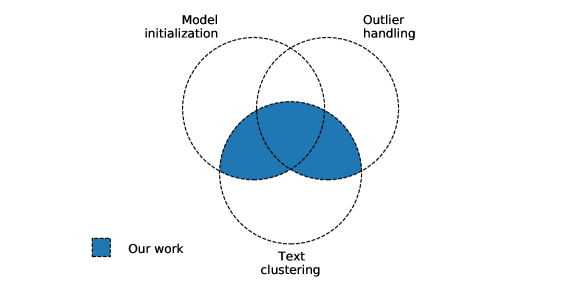
Figure 1: Venn diagram depicting how the present work is inserted into the central themes of “model initialization”, “outlier handling” and “text clustering”, indicated by the filled regions.

In this survey, we address two concerns in text clustering and topic modeling: initializing algorithms and detecting and handling unusual observations, commonly known as outliers or anomalies [23]. Figure 1 presents the Venn diagram of the scope of this literature review. Topic modeling handles several data types and can be part of frameworks (e.g., BERTopic [9]). However, we considered in Figure 1 that topic modeling is part of text clustering.

Some algorithms are sensitive to initial conditions or outliers, and the results may fall short of our expectations, or the optimization convergence rate may be compromised with weak initialization or biased toward a small number of instances whenever there are poor outlier detection and handling. The definition of “data outlier” is context-dependent [24, 25, 26], and “noise”, “anomaly” or many other terms are often treated as synonyms, although their exact meaning is not consensual [27]. Concerning topic modeling, “outliers” can also be defined at different levels: token, sentence, or topic level, which requires distinct approaches. While often thought of as undesired noise in data, many outliers need to be appropriately addressed, as they also represent the corpora structure, such as underrepresented topics [28] or rapidly emerging topics [29].

The benchmarks should provide sufficient variability (and difficulty levels) to assess the strengths and weaknesses of each outlier detection algorithm [30, 31] and fully recognize breakthroughs and advancements in the literature [32, 31]. Nevertheless, without robust benchmarks and with a smaller variability of datasets, the results can be excessively optimistic [32]. The benchmarks also must describe clear and concise evaluation criteria [31], and new algorithms may be tested using larger testbeds [33]. Notwithstanding the importance of the benchmarks, there is an absence of standardized evaluation metrics, inconsistencies in evaluation procedures, benchmarks, and pipelines [34, 12, 35, 36, 15, 37].

There are efforts to define the state-of-the-art (SOTA) of topic models [12]. However, establishing the SOTA can be misleading when the existing metrics cannot be suitable for the newest topic modeling algorithms [37]. Due to the ambiguity of human judgment toward automated metrics (e.g., coherence scores), it is uncertain whether a positive correlation between human evaluation and automatic metrics implies causality. Nonetheless, the inconsistencies in performance evaluation metrics are out of the scope of this survey.

To the best of our knowledge, there are neither surveys nor reviews concerning outlier detection and how to improve the quality of the initialization for text data for text clustering and topic modeling [8, 14, 16, 38, 39, 34]. Thus, this systematic literature review discusses outliers and initialization issues in the aforementioned context.

Our research questions are:

1. Which are the terminologies of the clustering, topic modeling, initialization, and outlier detection literature?

2. How does the literature address the randomness and, consequently, the reproducibility loss associated with initialization issues?

3. How does the literature address the distortion associated with outlier detection issues?

4. Which are the key factors that compromise scientific cooperation and decelerate the advancement of the research fields?

5. What research opportunities are there?

Our contributions to this work are:

1. To adapt the PRISMA SLR method to the domain of computer science research;

2. To summarize found initialization algorithms and outlier detection algorithms concerning topic modeling and clustering;

3. To clarify the terminology of the text clustering and adjacent subjects;

4. To present and summarize text clustering algorithms with their: theoretical background, adjacent algorithms, computational complexities, and limitations;

5. To point out research opportunities, and open issues for text clustering and topic modeling.

This work is organized as follows: Section 2 presents the information related to how we selected our reviewed works, the eligibility criteria, and synthesizes relevant characteristics from the selected works. Section 3 details the existing benchmarks with respect to outlier detection. Section 4 disambiguates outliers and details the algorithms that handle them. In Section 5, there are presented initialization issues and algorithms to mitigate the risk of weak initialization. Section 6 briefly reviews current end-to-end topic models. Section 7 presents general discussions of the reviewed works, research opportunities, and currently open issues. Section 8 describes other literature reviews for topic modeling and clustering. Appendix A presents the methods the reviewed algorithms used to vectorize the text data before the clustering or the topic modeling. Finally, appendices B and C introduce the foundations of factorization and clustering algorithms related to the reviewed works, respectively.

2 Methodology for the Work Selection

The SLRs enable the summarization of the current state of the literature concerning a predefined scope [4]. When synthesizing these studies, research opportunities and gaps in previous research can be identified, compared to primary research that does not answer these problems alone [4]. Despite the fact that PRISMA focuses on health sciences, this work adapted the method to computer science domain. Moreover, the PRISMA-P [40] provides a review protocol that enhances reproducibility, defines the scope of the review, provides guidelines to write the article, reduces the partiality, and plans the decision-making (e.g., eligibility and exclusion criteria, and data extraction).

In particular, this survey could not perform meta-analyses, which consist of statistical analysis aiming to generalize the results of independent studies [40], because the literature of topic modeling and clustering does not use comparable metrics, and there was no consensus about the most appropriate metrics to compare all approaches [34, 12, 35, 36, 15, 37].

This section is divided as follows. Subsection 2.1 presents our information sources, whereas the following defines the eligibility criteria and search strategy. The Subsection 2.3 presents our data extraction method, and the Subsection 2.4 summarizes information from our data extraction.

2.1 Information Sources

This literature review included three sources: ACLweb, Scopus and Web of Science. The ACLweb (anthology of the Association for Computational Linguistics (ACL)) comprises conference papers on computational linguistics. Scopus is a search engine that includes conferences and journals. There are rigorous criteria to select and index these publishers. Most of the highest cited conferences according to the H5-Index of Google Scholar are amongst the indexed proceedings of Scopus. The Web of Science is also a search engine with rigorous criteria and indexes mainly journals. This engine is responsible for the Journal Citation Report (JCR), an evaluation metric of the impact of journals and publishers. Finally, this review includes gray literature (e.g., book chapters) that may not be indexed in academic search engines.

2.2 Eligibility Criteria and Search Strategy

The authors used a snowballing search strategy to identify synonyms to complement the search string. The query for outliers included terms such as outlier, anomaly, abnormality, discordant, deviant, exception, peculiarity, aberration and surprise. Moreover, it considered clustering and topic modeling, including US and UK English particularities. There were also expressions concerning text data, which were natural language processing, NLP, and text mining. In the context of initialization, the string contained initialization, and analogously included expressions for clustering and NLP like in the outlier search string. There is a data extraction protocol to reduce variability, which is presented in Subsection 2.3.

The systematic review included all works retrieved in ACLweb, Scopus, and Web of Science. The exclusion criteria consisted of retrieved proceedings with full editions, duplicate works amongst search engines, and duplicate works between initialization and outlier search strings. Besides, there were included published works from 2011 up to November 2021 written in English, whose scope involved topic modeling, clustering or related algorithms, text data, outliers, or initialization (whether the work proposed specific algorithms that tackle these issues or defined them). The authors repeated the search to double-check the retrieved works. Some works were not retrieved in the second attempt, but they met the eligibility criteria. Therefore, they were included in this literature review. The articles whose download was unavailable with our licenses (the institutional one and another of a national research foundation) without available preprint versions were excluded. In addition, the authors used the same search strategy, regardless of the search engine.

The researchers included nine extra literature works (e.g., book chapters, surveys), even though they would be older than the 10-year time frame. Each screened paper was revised, at first, by one reviewer, in order to exclude the ones that were not eligible. The works that were ambiguous and the eligible ones were independently scrutinized by three reviewers, who did not have access to the others’ spreadsheets. After selecting, we calculated the kappa ($\kappa$) coefficient (see Equation 1). First, based on initialization, only works exclusively about this topic were considered, and the same occurred with the case of outliers. Nevertheless, we calculated the global $\kappa$ with all the selected works and all the eligible works, regardless of the groups they belonged to. The $\kappa$ for initialization was 68.00%, whereas the $\kappa$ outliers was 48.94%. The global $\kappa$ coefficient was 55.56%.

$$\kappa=\frac{\text{Selected works based on unanimity}}{\text{Eligible works}}*100\%$$ (1)

Despite the disagreement, the divergent decisions were analyzed individually by the reviewers’ panel. Finally, Figure 2 presents the diagram with the performed steps to screen the records and to select the eligible works about outliers and initialization. The analysis of three reviewers reduced the number of eligible works, and the sum of the remaining works and the included records are the total of selected works.

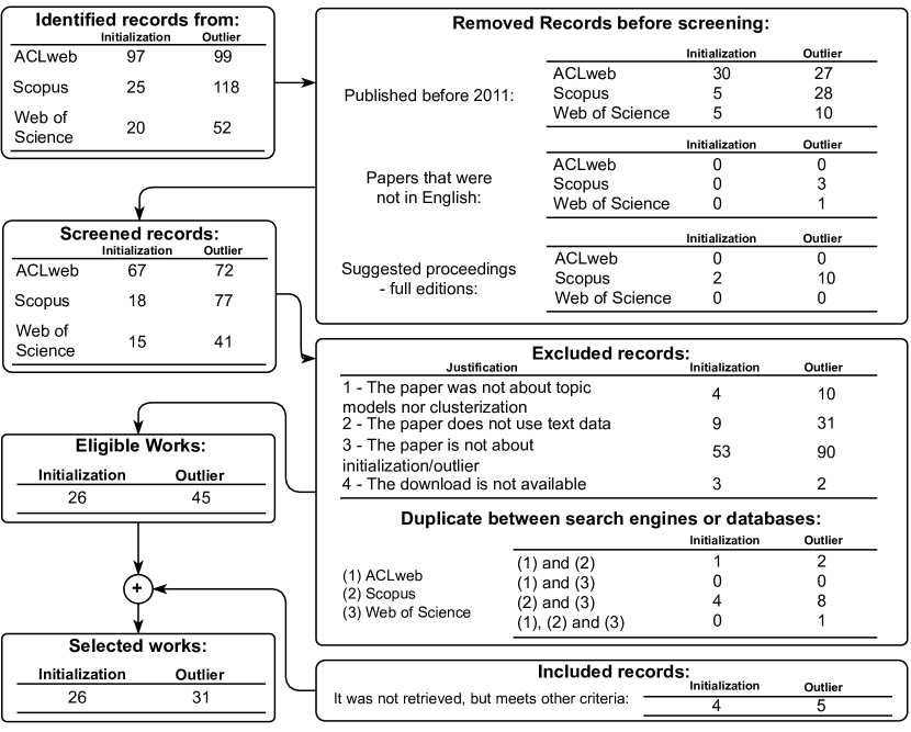
Figure 2: PRISMA flowchart for reviewed works.

2.3 Data Collection and Partiality Issues

The authors predefined a list of questions and topics to guide the data extraction and to mitigate the partiality. From the selected works, 30% were scrutinized by the reviewers to settle the data extraction process. The remaining 70% were divided equally amongst the reviewers.

The data were sought concerning: corpora, learning approach (unsupervised, supervised, or semi-supervised), complementary learning methods (e.g., active learning, reinforcement learning), clustering and topic modeling algorithms (including the number of clusters, geometry, and group balance), preprocessing methods, text vectors, metrics (performance, concordance, similarity, and dissimilarity), initialization and outlier concepts, user interaction, computational implementation, visualization tools, outlier detection and initialization algorithms, objectives of the works, findings, advantages, drawbacks and research opportunities. Furthermore, the data extraction process included all the selected works. Each reviewer had tables to fill in the information about each paper. Besides, there could be appended remarks or citations that the reviewer considered necessary for each reviewed work. The collected data are presented throughout this review paper, summarized by the authors. Finally, the reviewers included “not mentioned” to the corresponding gap in the data extraction tables to enhance traceability whenever there was missing information.

2.4 Synthesis of Reviewed Algorithms

This subsection synthesizes relevant reviewed work characteristics. They are categorized from different perspectives, aiming to improve the understanding of which techniques and algorithms the topic modeling research area has been using recently, also emphasizing outlier handling and initialization strategies for one or more components in a typical topic modeling pipeline.

Clustering algorithms are commonly found in the core of topic modeling pipelines, alongside proper probabilistic models designed for such task and factorization algorithms. The K-means algorithm is a popular baseline algorithm to evaluate more sophisticated algorithms. Table 1 summarizes the common clustering or topic modeling algorithms among the reviewed works.

Table 1: Reviewed works categorized by clustering or topic modeling algorithms they consider in their experiments. Some works may appear in multiple categories. “DBSCAN” stands for “Density-based Spatial Clustering of Applications with Noise”, ‘PAM” for “Partition Around Medoids”, “LDA” for “Latent Dirichlet Allocation”, “LSA/LSI” for “Latent Semantic Analysis/Indexing”, “NMF” for “Non-negative Matrix Factorization”, and “pLSA/pLSI” is the probabilistic LSA/LSI.

Clusterer/ Topic Model	Works
DBSCAN	[41, 42, 43]
Hierarchical	[44, 29, 45, 7, 46, 47, 43, 48]
K-means	[49, 50, 51, 7, 52, 53, 54, 5, 23, 42, 43, 55, 56, 57, 47, 58, 59]
K-medoids (PAM)	[56, 23, 7, 60]
LDA	[61, 62, 56, 63, 64, 65]
LSA/LSI	[66, 5, 43]
NMF	[54, 55, 59, 67]
pLSA/pLSI	[28, 64]
Others	[68, 44, 69, 70, 71, 62, 5, 63, 72, 59, 41, 58]

Some algorithms popularly used in topic modeling are sensitive to initial conditions, such as K-means [43, 5] or NMF [67]. Some reviewed works run multiple random initialization, selecting the best at the end according to particular criteria, or proposing algorithms to initialize their clustering models in an informed way. All revised works that developed their initialization strategies are summarized in Table 2. For the sake of brevity, models initialized from publicly available pretrained weights were omitted from this table but included in Table 4.

Table 2: Reviewed works grouped by initialization. Some works may appear in multiple categories. All categories may include randomness but differ by using a more complex or informed initialization procedure. “Multi-stage heuristics” category comprises works that explicitly described their initialization procedures in two or more stages.

Initialization category	Works
Multi-stage heuristics	[60, 64, 43, 5, 59, 56, 73, 71]
Random (multiple seeds)	[42, 62, 67, 59, 52]
Random (single seed)	[55, 53]
Others	[55, 67, 58, 57, 65]

From all the 57 works considered, 31 (54%) handled outliers during the experiments, whereas only 16 (52%) of them clearly defined what an “outlier” is. Those definitions vary considerably from work to work, from more general ones (e.g., “instances in low-density regions”) to definitions specific to text data (e.g., “topic that does not belong to the given text document”). The strategies that adopted the outlier handling range from pure similarity analysis (e.g., cosine similarity distribution) to density-based algorithms (e.g., Local Outlier Factor (LOF) [74]). Five works proposed original algorithms robust to outliers by design so that the outliers would not compromise the results. The outlier handling strategies for each work can be seen in Table 3.

Table 3: Outlier handling among the reviewed works. Some works may fit into multiple categories.

Outlier handling strategy	Works
Density-based	[42, 75, 72, 46, 70, 48, 76, 77, 78, 57]
Robust to outliers by design	[79, 54, 57, 43, 63]
Similarity-based	[80, 81, 21, 66]
Others	[62, 61, 50, 29]

Working with text data requires embedding of words, sentences, or documents into a vector space model as numerical vectors to enable optimization over the data. Among the reviewed works, Term Frequency-Inverse Document Frequency (TF-IDF) [82, 83, 84] was the most common vectorization technique, used by 17 (30%) works, followed by 11 (19%) works using Bag-of-words (BOW) or Bag-of-$n$-grams, and word2vec [85] and [86] was found in 9 (16%) works. Other embedding strategies used in two or more reviewed works were GloVe (Global Vectors) [87], doc2vec [88], Latent Dirichlet Allocation (LDA) [22] or Non-negative Matrix Factorization (NMF) [89, 90] (both as intermediary representations) and fastText [91, 92, 93]. Table 4 summarizes these findings.

Table 4: Identified embedding methods for all reviewed works. Some works may appear in multiple categories as they experimented with different embedding methods. “LDA” and “NMF” works listed here used these algorithms to generate intermediary representations in the topic modeling pipeline, even though they require preliminary data embedding.

Embedding method	Works
BOW/Bag-of-$n$-grams	[7, 42, 94, 79, 46, 54, 41, 61, 47, 95, 53]
doc2vec	[72, 77, 78]
fastText	[96, 78]
GloVe	[44, 62, 21, 81, 80]
LDA	[61, 56, 52, 28, 97]
TF-IDF	[7, 42, 55, 67, 21, 59, 71, 50, 29, 77, 57, 63, 66, 5, 49, 58]
Transformer encoder	[9, 97, 95]
word2vec	[80, 98, 53, 51, 81, 65, 78, 69, 63]
Others	[44, 75, 70, 48, 43, 64, 5, 63]

From the 40 (70%) reviewed works that reported empirical results, the most common metrics were accuracy, precision, recall, F1-score (harmonic mean of precision and recall), and Normalized Mutual Information (NMI) [99]. When NMI is normalized by the arithmetic mean of cluster assignment entropy from two distinct sources, it is equivalent to the V-measure (harmonic mean of cluster assignment completeness and homogeneity) [100]. Adjusted Mutual Information (AMI) [101] is an NMI variant where the measure expected value for random agreement is accounted for, a useful property when the ratio of instance count to the number of clusters is small. Note that both NMI and AMI correspond to a family of related metrics as the normalization strategy varies (see [99, 101]). Hence comparing reported results from distinct works needs to be done carefully.

The accuracy and F1-score were used mainly for supervised proof of concept studies of unsupervised algorithms. Only 4 reviewed works used statistical tests to validate their results [46, 5, 58, 77]. From the 30 (53%) works that developed their data preprocessing steps, the most common choices (besides text tokenization) were text cleaning (e.g., removing unwanted symbols), stopword removal, stemming, and case-folding. When analyzing their results, tables, line graphs and flowcharts were predominant. Figure 3 summarizes these findings.

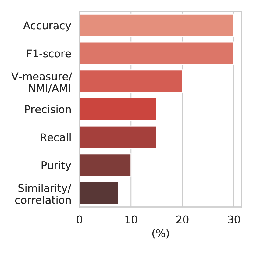
(a) Evaluation metrics.

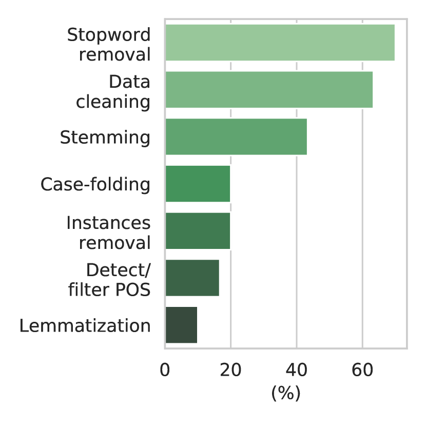
(b) Preprocessing methods.

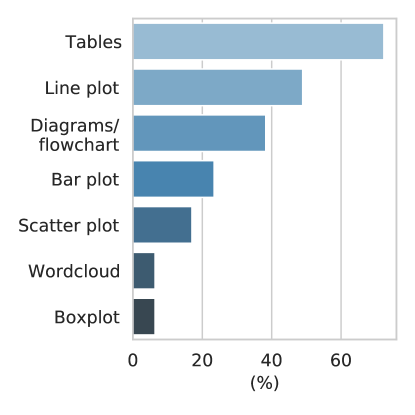
(c) Visualization tools.

Figure 3: Percentage of metrics (Figure 3(a)), preprocessing methods (Figure 3(b)), and visualization tools (Figure 3(c)) from the reviewed works that reported these data.

Table 5: Programming languages and reviewed works with available implementations. Some publications provided implementations in more than one language.

Programming Language	Works
C/C++	[45]
Java	[73]
Matlab	[59, 23, 79]
Python	[53, 80, 23, 81, 45, 69, 44, 50, 9, 97, 73, 95]
R	[23, 73]

Table 5 summarizes the works with available implementations. Only 14 works (from 57 reviewed works, which included the gray literature and papers that could not be retrieved but met the criteria) provided their implementations, hindering the research area efforts by reducing reproducibility.

The machine learning paradigms used by the reviewed works were unsupervised as the predominant paradigm with 49 (86%) works, followed by supervised learning with 6 (11%) works, and, finally, semi-supervised learning with 3 (5%), considering that few works used multiple paradigms.

3 Outlier Detection Benchmarks

In 2016, [30] surveyed general-purpose unsupervised algorithms based on k-nearest neighbors to create a benchmark. [102] also addressed unsupervised anomaly detection, dividing the algorithms into nearest-neighbor based, clustering-based, statistical, subspace-based, and classifier-based/other. [32] presented a meta-analysis of outlier detection algorithms and the existing benchmarks. [103] and [104] also developed benchmarks to the unsupervised outlier detection problem. In 2021, [31] surveyed shallow and deep outlier detection algorithms, dividing them into classification-based, probabilistic, reconstruction-based, and distance-based. Next, [105] analyzed the problem of how to fine-tune and select the hyperparameters of unsupervised outlier detection algorithms. Finally, in 2022, [33] proposed a new benchmark concerning anomaly detection, with the perspective of the levels of supervision, the contamination of data, and the types of anomaly (e.g., local, global, group anomalies, and dependency anomalies), using the default hyperparameters.

[102] and [31] mentioned the problem of the curse of dimensionality when dealing with high-dimensional data, which is a frequent concern in NLP. The eight benchmarks analyzed in this survey were focused on tabular data. In 2022, [33] is the first work to consider NLP datasets (4 amongst the 55). These text data were embedded with Bidirectional Encoder Representations from Transformers (BERT) [106], extracting the [CLS] token. [32], [104], [31] and [33] used synthetic data. The strategy of downsampling was used to create outliers in works like [30, 33]. [104] provided an in-depth analysis concerning the synthetic datasets.

With the type of the outlier known in advance [30, 102, 33] or the context of the dataset [32], it is possible to define well-tailored decision-making concerning the outlier detection algorithms [30]. Besides, the data properties (e.g., dimension, number of instances, scale, hierarchy, contamination, context, and so forth), domain, and application sustain assumptions about the choice of the algorithms [31]. [105] advocated that it is not possible to compare performance metrics when some papers use the default settings, whereas others set different hyperparameters. Furthermore, the fine-tuning influenced the algorithm performance, and some anomaly detection algorithms cannot be tuned due to the computational overhead [105]. In addition, datasets with only 100 labeled instances with anomalies (called validation set) led to a performance gain [105]. According to [33], the use of feature selection techniques can mitigate the influence of noisy data.

During the evaluation, the benchmarks used as their performance metrics the Precision at n (P@n) [30, 31], Adjusted P@n [30], Average Precision [30, 32, 103, 31], Area Under the Curve of the Receiver Operating Characteristic Curve (ROC AUC) [30, 102, 32, 103, 104, 31, 105, 33], Area Under the Precision-Recall Curve (PR AUC) [103, 104, 31, 33], and Average AUC [105]. According to [31], the PR AUC is a better performance metric than ROC AUC, since ROC AUC can be overly optimistic. Finally, [30, 104, 33] concluded that, with their experiments, no anomaly detection algorithm outperformed the others regardless of the scenario, type of outlier, or dataset characteristics.

4 Outlier Detection and Handling

The exact definition of “outlier” can be difficult because it highly depends on the task context [24, 25]. For instance, in the context of Hierarchical Agglomerative Clustering (HAC), while [6, p.382] claims that complete-linkage is “sensitive to outliers”, in [107, p.558] and [108, p.283–284] the complete-linkage is said to be “more robust to outliers” while single-linkage is sensitive to it. In [109, p.533], the single-linkage is again said to be “robust to outliers”, but sensitive to “errors of measurement”. Since the single-linkage is more susceptible to the chaining effect, and the complete-linkage uses the maximum pairwise distance between clusters, both can have undesired effects due to data points in low-density regions. However, they do not share the same problem in a general sense. Hence, while the descriptions of these works use the same keyword “outlier”, they do not describe the same issue. Some authors claim that other common names for outliers in the literature are novelty, abnormalities, discordants, deviants and anomalies [26] and potentially many others, but whether all these terms actually refer to the same phenomena is not consensual [27]. These issues highlight the importance of a clear definition of what “outlier” is in the context of each separated work.

In the context of text data, outliers may be defined in word, sentence, or document level. Concerning topic modeling, outliers can be defined in the topic level, such as underrepresented topics [28] or topics that expand too fast [29]. From the reviewed works, 16 (52%) works defined what an “outlier” means in the context of their experiments, from 31 total works that handled outliers. The majority of these works defined outliers in the document level. Documents that deviate from corpus distribution in a perceptive manner are a common definition pattern. Just a few works defined outlier in the word level [80, 81, 61] and in the topic level [29, 62, 28].

For the rest of this section, we will present a few techniques and algorithms regarding outlier handling, detection, or removal found in reviewed works.

Either similarity or density-based outlier detection methods need to compare embeddings. One common choice of similarity function is the cosine similarity between a pair of embeddings $a$ and $b$ [80, 66, 57, 42, 75, 70], as shown in Equation 2.

$$\operatorname{similarity}(a,b)=\cos(a,b)=\frac{a^{T}b}{\left\|a\right\|_{2}\left\|b\right\|_{2}}=\frac{\sum_{i}a_{i}b_{i}}{\sqrt{\sum_{i}a_{i}^{2}\cdot\sum_{i}b_{i}^{2}}}$$ (2)

Based on [110] and [111], in the reviewed work [81], a rank-based alternative (called APSync) for cosine similarity was proposed. It was shown to consistently outperform cosine similarity in outlier detection experiments. The APSynP definition is shown in Equation 3, where $\operatorname{rank}(v_{i};v)$ denotes the index that $v_{i}$ falls when entries in vector $v$ are sorted decreasingly, and $p\in[0,1]$ is a hyperparameter and fixed as $p=0.1$ in the paper experiments based on empirical validation.

$$\operatorname{similarity}(a,b;p)=\text{APSynP}(a,b;p)=\sum_{i}\frac{2}{\operatorname{rank}(a_{i};a)^{p}+\operatorname{rank}(b_{i};b)^{p}}$$ (3)

The reviewed work [66] proposes to use Angle-Based Outlier Factor (ABOF) [112], which analyzes the variance between the angles of documents in the embedded corpus to identify “outlier documents”, or documents consistently farther away from all other documents. The hypothesis behind this method is that, for a sufficiently farther away observer (an outlier), every other document is next to each other, and hence the variance of the angles between the observer and every other documents is small. This idea is formalized in Equation 4 which calculates the ABOF for a single document $d$, where VAR denotes the empirical variance.

$$\text{ABOF}(d;D)=\mathop{VAR}_{i,j=1,\ldots,\lvert D\lvert}\left[\frac{(d-d_{i})^{T}(d-d_{j})}{\|d-d_{i}\|_{2}^{2}\|d-d_{j}\|_{2}^{2}}\right]$$ (4)

Clustering is commonly at the core of topic modeling algorithms. Thus, it may be relevant to choose a clustering algorithm that is insensitive to outliers or can handle unusual observations during the execution. Classical clustering algorithms such as PAM, Clustering LARge Applications (CLARA), and Clustering Large Applications based on RANdomized Search (CLARANS) are potentially robust to outliers (if a proper similarity function is chosen), while DBSCAN and Hierarchical DBSCAN (HDBSCAN) are able to handle outliers naturally, although in this case outliers are often considered undesired noise instances in the data. Since these algorithms are employed to cluster documents or words, the outlier detection is often restricted to word and document levels and not to the topic level.

In [42], classical K-means and intra-cluster similarity were combined, where documents that have low similarity with their respective centroids are considered outliers. In [70], a similar approach was taken when documents were first clustered in two clusters and afterward may be reassigned to the other cluster grounded on which cluster the document has higher cosine similarity.

In [29], rapidly emerging topics are considered outliers. This approach differs from the majority of other works since it is applied to data streams. For each topic $w$ in a vocabulary V, represented as word $n$-grams, its significance score is calculated as shown in Equation 5, where $f:V\rightarrow\mathbb{R}_{+}$ maps each topic to its frequency, $\mu,\sigma^{2}:V\times\mathbb{N}\rightarrow\mathbb{R}_{+}$ are the moving average and variance of the topic frequency respectively, $\eta>0$ is a learning rate for both moving statistics, and $\beta>0$ is a bias term that avoids division by zero and also smooths the formula to be more robust to rare terms.

$$\text{significance}(w,t;f,\eta,\beta)=\frac{f(w)-\max\left\{\mu(f(w),t;\eta),\beta\right\}}{\sqrt{\sigma^{2}(f(w),t;\eta)}+\beta}$$ (5)

If a topic $w$ has a significance level above a threshold $T=\mu+s\sigma^{2}$ for some predetermined $s>0$, then $w$ is considered an outlier (rapidly emerging topic). As it handles data streams, the significance level is checked periodically.

In [72], Fuzzy K-means was used to detect outlier documents. More precisely, the Fuzzy K-means (see the objective function in Equation 32) is run in the corpora embedded with doc2vec, and documents close to the cluster decision boundaries are considered potential outliers and inserted into a subset $O$. Then, the Fuzzy K-means is rerun into $O$, and every outlier candidate that sufficiently increases the objective function is declared an outlier by the algorithm.

In [63], a probabilistic generative algorithm is proposed for topic modeling similar to LDA called Embedded von Mises-Fisher Allocation (EvMFA), by using embeddings from word2vec as input to the generating process, therefore generating documents as a bag-of-normalized-embeddings instead of a bag-of-words similar to LDA by following a von Mises-Fisher distribution (the Gaussian distribution analog in directional statistics) instead of a categorical distribution for each word. Equation 6 shows the probability density function for von Mises-Fisher distribution, where $i$ is the topic index, $d\in\mathbb{N}^{E}$ is a $E$-dimensional embedded document, $\kappa>0$ is the concentration parameter (thus inversely proportional to the variance), $\mu_{i}\in\mathbb{R}^{E}$ is the mean direction for topic $i$ such that $\|\mu_{i}\|_{2}=1$, and $I_{z}$ is the modified Bessel function of the first kind at order $z$.

$$p\left(d;\kappa_{i},\mu_{i},E\right)=\frac{\kappa_{i}^{(E/2-1)}}{(2\pi)^{E/2}\cdot I_{(E/2-1)}(\kappa_{i})}\exp(\kappa\cdot\cos(\mu_{i},d))$$ (6)

Similar algorithms were previously used in [113, 114] also for topic modeling, but [63] focuses its application on outlier detection. First, it uses EvMFA to model the topic regions, or semantic focus regions. Then, it filters out regions with low concentration (low estimated $\kappa$) grounded on a hyperparameter $\beta\in[0,1]$, which corresponds to a cutoff to the semantic focus cumulative probability distribution. Lastly, it uses a criterion named Orthodox Quantile Outlierness (OQO) $\Omega(d;\theta)$ to compute the probability of whether a document is an outlier, based on how many orthodox tokens compose it. Orthodox tokens are tokens that both are found close to semantic focus areas and also sufficiently specific to corpus $D$ against a background corpus $D_{\text{bg}}$. Equation 7 shows the OQO criterion, where $q(\,\cdot\,;\theta)$ denotes the $\frac{1}{(1-\theta)}$-quantile function of Poisson-Binomial distribution, and $\omega_{\text{orthodox}}$ is a function that estimates the orthodox token count within document $d\in D$ against a background corpus $D_{\text{bg}}$.

$$\Omega(d;\theta,D,D_{\text{bg}})=1-\frac{q(\omega_{\text{orthodox}}(d;D,D_{\text{bg}});\theta)+1}{\lvert d\lvert+1}$$ (7)

Other general-purpose outlier detection algorithms were also employed in the reviewed works: Local Outlier Factor (LOF) [74] was present in 3 works [46, 77, 78], One-class Support Vector Machine (One-class SVM) [115] in 2 works [65, 94] and Isolation Forest [116, 117] used in a single work [50]. All these algorithms are available in the scikit-learn library [118, 119].

In [79], an NMF variant ("Text Outliers using Nonnegative Matrix Factorization (TONMF)") was developed to detect outlier documents. The objective function resembles Equation 26, but assumes that $D=L_{0}+Z_{0}$, where $Z_{0}$ is a matrix of outlier factors and $L_{0}$ is the true document embeddings generated by an underlying process. Thus, the new objective function is given by Equation 8.

$$\begin{split}\min\limits_{W,H,Z}J(W,H,Z;D,\alpha,\beta)&=\min\limits_{W,H,Z}\tfrac{1}{2}\left\|D-WH-Z\right\|_{F}^{2}+\alpha\left\|Z\right\|_{(2,1)}+\beta\left\|H\right\|_{1}\end{split}$$ (8)

subject to $$\quad W,H\geq 0$$

In this equation, $\alpha\geq 0$ controls the sensitivity of the algorithm for outliers, $\beta\geq 0$ is a regularization factor to provide sparsity to the results, and $\left\|\,\cdot\,\right\|_{(p,q)}$ is a matrix-mixed norm defined in Equation 9. During the experiments, the authors noticed that $\beta$ has low influence in the results.

$$\left\|Z\right\|_{(p,q)}=\left(\sum_{i}\left(\sum_{j}\lvert z_{(i,j)}\lvert^{p}\right)^{\frac{q}{p}}\right)^{\frac{1}{q}}$$ (9)

Unlike the original paper that defines $D$ so that each column corresponds to a document, in the present work, $D$ is defined such that each document is represented by a row, and hence the mixed-norm term in Equation 8 was adapted to reflect our convention. After the optimization procedure, the $\ell_{2}$-norm from the rows of the outlier matrix $Z$ are calculated, and documents with high scores are considered outliers by this particular method.

Another NMF variant called $\ell_{1}$-norm Symmetric Nonnegative Matrix Trifactorization ($\ell_{1}$ S-NMTF) was proposed in [54] to perform NMF while effectively handling outlier documents during the optimization process, showing noticeable improvements over vanilla NMF and other algorithms in their experiments. The authors also provide an optimization algorithm. The drawback of this method is that it requires a particular representation of $D$.

The reviewed work [61] pointed out that a small amount of data available leads to less coherent and interpretable topics. To cope with this, they used Regularized LDA [120], which also improves results for text with noise. It works by choosing specific priors based on statistics of external, sufficiently large corpora $D_{\text{external}}$, and plugging it into the traditional LDA. More precisely, a “covariance” matrix $C=WW^{T}$ is computed, where $W$ is a co-occurrence matrix of top-$k$ most current words from $D_{\text{external}}$ within a moving window through the documents. It was shown in the original paper to improve mutual information against human judgment for topic modeling and may decrease model perplexity slightly.

The reviewed work [62] uses Convolutional Neural Networks (CNN) [121, 122] algorithms combined with scores from BM25 [123] to detect unrelated topics to a given document, the intruder topic, from a list of candidate topics that may belong to the document. Unlike most reviewed works, this one adopts the supervised learning paradigm for outlier topic detection.

5 Initialization of Topic Modeling and Clustering Algorithms

Topic models often have components sensitive to initialization settings, which raises the question of what is the best initialization strategy. A straightforward strategy is to initialize each component multiple times with distinct random initialization and pick the setting that gives the best performance according to some metric(s) [42, 62, 67, 59]. While simple, this strategy may not be deployed for expensive pipelines. This section groups strategies from the reviewed works to initialize common components of topic modeling pipelines, which are designed to be either more robust to outliers or to improve the optimization convergence rate.

K-means++ [124] consists of the regular K-means with an initialization algorithm proposed to reduce the variability of the clustering result. It works by sampling the initial centroids iteratively while taking into account the centroids already selected under the hypothesis that centroids are better initialized far apart from each other. Choosing iteratively always the farthest possible data points from the current centroids is an approach sensitive to outliers. Thus, the K-means++ approach selects them randomly. The first centroid $c_{1}$ is taken arbitrarily. Then, each document $d$ in $D$ has a probability inversely proportional to the squared Euclidean distance to the closest centroid to become the next centroid, as shown in Equation 10, where $C$ is the set of centroids currently chosen.

$$p(d\lvert C;D)=\frac{\min\limits_{c\in C}\|d-c\|_{2}^{2}}{\sum\limits_{z\in D}\min\limits_{c\in C}\|z-c\|_{2}^{2}}$$ (10)

This process is repeated $k-1$ times until the requested number of centroids $k$ is gathered. After this initialization procedure, the regular K-means is run. From the reviewed works, 3 works used K-means++ in their experiments [52, 56, 43] (corresponding to 18% of works that used K-means).

The reviewed work [56], when initializing K-medoids, closely follows Equation 10 by replacing centroids with medoids, an idea which was considered by [125]. However, [126, 73] show that such a strategy may impair PAM convergence rate and propose a PAM initialization named Linear Approximative BUILD (LAB), where it applies the original PAM initialization algorithm BUILD with subsamples of size in $\mathcal{O}(\lvert D\lvert^{\frac{1}{2}})$. For computationally cheaper versions of PAM, such as FasterPAM, the initialization procedure is often associated with the largest portion of computational cost rather than the algorithm optimization steps. Thus, cheaper initialization like K-means++ is preferred, even though it is less reliable than the costly but precise BUILD method [73].

Even though K-means++ is a better initialization algorithm than random initialization, [127] argues that it is too sensitive to outliers. For this purpose, they propose the Thresholded K-means++ (T-kmeans++), which essentially sets an upper bound to the distance between each point and the currently chosen centroids before computing the K-means++ sample probabilities, thus reducing the probability of outlier centroids as shown in Equation 11, where $T$ is a given threshold.

$$p(d\lvert C;D,T)=\frac{\min\limits_{c\in C}\left\{\|d-c\|_{2}^{2},T\right\}}{\sum\limits_{z\in D}\min\limits_{c\in C}\left\{\|z-c\|_{2}^{2},T\right\}}$$ (11)

In [57], a K-means initialization method called WIKTCM, which considers possible outliers, is proposed. The first centroid document is the document with the highest total similarity to all other documents. Then, the next centroid documents are chosen deterministically and iteratively grounded on a score proportional to the similarity score to all other remaining, non-outlier documents and also proportional to the dissimilarity with previously chosen centroids, as shown in Equation 12, where $C$ denotes the set of previously chosen centroids, and $O$ denotes the set of currently identified outlier documents.

$$c_{\text{next}}=\operatorname*{argmax}\limits_{d\in(D-C-O)}\underbrace{\left[\frac{1}{\lvert D-C-O\lvert-1}\sum_{z\in(D-C-O)}\cos(d,z)\right]}_{\text{Average similarity with remaining documents}}\cdot\underbrace{\left[\vphantom{\frac{1}{\lvert D-C-O\lvert-1}\sum_{z\in(D-C-O)}\cos(d,z)}\sum_{z\in C}1-\cos(d,z)\right]}_{\text{Dissimilarity to centroids}}$$ (12)

The outliers are detected before every new centroid is chosen based on their average similarity score to all remaining documents (non-centroids and non-outliers). If a document has average similarity below a threshold, it is considered an outlier and thus removed from corpus.

Finally, in [52], an influence graph-based initialization algorithm to the K-means was proposed, where this work claims improvements over the K-means++ initialization in its experiments using an algorithm of $\mathcal{O}(N\lvert E\lvert^{2}\lvert D\lvert^{-1})$ time complexity (where $N$ is the maximum number of iterations and $\lvert E\lvert$ the number of edges) called MMSE-2, corresponding to the objective function shown in Equation 13, the sum of squared errors of the approximated influence probabilities $p_{2}(d_{i}\ \rightarrow\ d_{j})$ for every weighted graph edge $(d_{i},d_{j},w_{(i,j)})\in E$, where $w_{(i,j)}\in[0,1]$, $NN(d;D)$ denotes the set of neighbor indices to document $d\in D$ and the similarity function is arbitrary as long as it maps any pair of documents to the $[0,1]$ range. This objective can be minimized using gradient descent.

$$J(W;D,E)=\sum_{(d_{i},d_{j},\cdot)\in E}\Bigl{(}\underbrace{1-\prod_{z\in\text{NN}(d_{i};D)\cap\text{NN}(d_{j};D)\\ }(1-w_{(i,z)}w_{(z,j)})}_{p_{2}(d_{i}\ \rightarrow\ d_{j})}-\underbrace{\vphantom{\prod_{d_{k}\in\text{NN}(d_{i};D)\cap\text{NN}(d_{j};D)\\ }(1-w_{(i,k)}w_{(k,j)})}\operatorname{similarity}(d_{i},d_{j})}_{\in[0,1]}\Bigr{)}^{2}$$ (13)

There were efforts to address the NMF sensitiveness to the initial conditions [67, 58, 20] in [128] whose propositions were three algorithms based on SVD (see Equation 24) to initialize matrices $W$ and $H$, namely Nonnegative Double Singular Value Decomposition (NNDSVD), NNDSVD Averaged (NNDSVDa), and NNDSVD Averaged Random (NNDSVDar). The first variant is suitable when sparseness in $W$ and $H$ is desired, and the last two make $W$ and $H$ denser with deterministic and random approaches, respectively. This algorithm is adopted in two reviewed works [58, 55]. Although these initialization algorithms were shown to improve the NMF convergence rate considerably, it is not clear if they perform any better than random initialization given enough iterations. These three initialization algorithms are available for the NMF implementation in the scikit-learn library [118, 119].

The reviewed work [55] also experiments with two other initialization algorithms for the NMF proposed in [20] grounded on semi-informed NMF random initialization. Its experiments show that NNDSVD is the most accurate but also the slowest initialization algorithm. Although less accurate, the other two are significantly faster and also provide improvements over uninformed random initialization. This work also shows that the best NMF initialization may depend on which algorithm solves the NMF optimization problem and also on the data distribution. The implementation of these three algorithms is available at the Nimfa library [129].

For neural-based text embedding initialization, it is common to adopt publicly available pre-trained embeddings from surrogate tasks with huge, general-purpose corpora, thus leveraging natural language understanding from typically richer data than the available for the downstream task. The transfer learning enables these embeddings to be fine-tuned during the downstream task optimization. The algorithms word2vec, doc2vec, and fastText and their respective pre-trained embeddings for varying dimensions are available in Gensim library [130], alongside all the datasets used for training. Pre-trained GloVe embeddings are also available online. Pre-trained transformers-based models (such as BERT and Sentence-BERT (SBERT)) are available in HuggingFace’s hub [131].

While embedding fine-tuning details is out of the scope of this present work, it is worth mentioning that often there is room for improving embedding quality for downstream tasks by fine-tuning to domain-specific data. For some distributed representations such as word2vec, doc2vec, and fastText, the same self-supervised algorithm can be used for such fine-tuning. For pre-trained embeddings originally from a supervised task such as SBERT, it is not obvious how to perform the fine-tuning since domain-specific labeled data may not be readily available. For such occasions, self-supervised contrastive learning algorithms are good candidates, such as Simple Constrastive Sentence Embedding (SimCSE) [132] or Contrastive Tension [133].

6 Topic Modeling as a Pipeline: End-to-End Topic Models

Current end-to-end topic models may rely on transformer encoders integrated with another topic modeling, clustering, and embedding algorithms.

BERTopic [9] is a topic modeling package that proposes creating topics from pre-trained SBERT document embeddings in a pipeline composed by dimensionality reduction with Uniform Manifold Approximation and Projection (UMAP) [134], followed by document clustering with HDBSCAN, and then topic extraction using the so-called class-TF-IDF, which consists of regular TF-IDF (see Equation 14) applied separately for each identified cluster from HDBSCAN. Since HDBSCAN identifies candidate outlier documents, the BERTopic proposed pipeline takes them into consideration as well, however assuming outlier documents are noise and thus are not modeled.

tBERT [97] concatenates contextual embeddings from BERT and traditional topic embeddings from algorithms such as LDA, further passed to a linear layer and a Softmax activation. Although this framework relies on topic extraction, its main purpose is to solve semantic similarity tasks between pairs of documents and not topic extraction.

Combined Topic Model (CTM, not to be confused with Correlated Topic Models) [95] concatenates pre-trained contextualized embeddings from SBERT and BOW embeddings in a Variational Autoencoder (VAE) [135] grounded on the idea of Autoencoded Variational Inference for Topic Model (AVITM) proposed by [136] and its Product of Experts LDA (ProdLDA), an extension of traditional LDA to a variational neural setting. Its results demonstrate that combining both SBERT and BOW may impact the topic coherence positively.

7 Discussion and Research Opportunities

The reviewed works did not use reinforcement, active or other machine learning paradigms for clustering or topic modeling tasks, which seem to be promising for text clustering research. For instance, the combination of neural topic modeling and reinforcement learning presented encouraging results [137]. Furthermore, associating active learning with text clustering can also result in better performance metrics [138]. Besides, there are research opportunities pertaining to the automated machine learning field, particularly hyperparameter optimization approaches, such as Bayesian hyperparameter optimization [35]. In the context of transfer learning, there are also applications to clustering tasks [139, p.48]. Moreover, when analyzing the algorithmic complexity, it would be more fair considering ranges of the inputs, length of the text vectors, or whether there are underrepresented topics (e.g., based on ground-truth labels) when choosing the most suitable algorithm for each task, instead of raw statistics of the asymptotic behavior of best, average or worst cases of the implementations. The inclusion of the likely impact of large constants on the processing time during the decision-making may improve the use of computational resources.

Since it is hard to match human intuition for topic models by automated optimization [11, 17], users may help the modeling algorithm by giving active feedback during the optimization process. This resource was not considered in the reviewed works, which seems to reflect research opportunities of interactive topic modeling and interactive outlier handling. For instance, interactive topic modeling pipelines may be employed in areas where the typical user will not have machine learning expertise to tune the model hyperparameters by hand or provide the necessary modifications directly to reflect its objectives [140]. Concerning initialization, the seeding process presents itself as an alternative to more efficient approaches. The seeding process consists of methods to cherry-pick more favorable elements to begin the clustering or topic modeling to yield faster convergence, better performance, and lower computational costs. This process can be improved whenever an oracle is available (e.g., user interaction and semi-supervision). In addition, the gains provided by methods that are robust to initialization settings and the ones that arise from better seeds need to be compared. Finally, some criteria can address the specificity of the number of seeds depending on corpus size, text domain, and algorithm.

Besides, the evaluation of topic models and clustering methods that do not use a predefined number of groups can be challenging. If a method obtains more groups than the ground-truth labels (whenever a labeled corpus is available), it can mean that the modeled groups are overly specific. Nonetheless, there are challenges to be addressed, including: partitioning criteria; cluster granularity; comparison of ground-truth labels and the obtained clusters (even though there are different numbers of groups); acceptability of smaller or bigger groups in comparison to the original labels; penalization of outliers mistakenly grouped; balance of the trade-off concerning the mistakes of clustering outliers or gathering instances that belong to other groups; analysis of the correspondence between predicted and actual groups; and the fine-tuning of hyperparameters albeit the inconsistency of performance metrics.

Despite machine learning not having silver bullets, developing and testing approaches to evaluate topic models and clustering algorithms assesses structured and effective cooperation and development of text clustering research. There is a need for benchmarks that include metrics and corpora, which was also reported in [12, 35, 36, 15]. New topic models had been released in 2021. Nevertheless, due to the absence of baselines and standardized benchmarks [15], defining the state-of-the-art is not a trivial task. Thus, this cumbersome issue hinders the advancement of research, leading to rework and unrealistic performance gains (mainly when there is no statistical analysis). The literature of text clustering and topic models would benefit from the definition of corpora to enable benchmarks concerning different text domains and lengths, the study of the influence of text length or its domain on the language models (LMs) and their relation with clustering quality, and the determination of standardized metrics that can be applied to older topic modeling algorithms (e.g., LDA) and to new ones (e.g., neural topic models) [37].

NMF and LDA rely on the document-term matrix to represent the text, while clustering methods such as K-means and HDBSCAN can use more general embeddings. These vectors can be sparse, and the curse of dimensionality can hamper the algorithm performance when the vector length is bigger than the corpus size. As a result, dimensionality reduction arises as an alternative to improve these algorithms. Defining the best algorithms to text data, fine-tuning their hyperparameters, and reducing their stochasticity may lead to performance gain.

Methods whose objective solely relies on anomaly detection (e.g., IF, LOF, and One-class SVM) require tuning to the corpus characteristics. Understanding the best moment to detect outliers (either before clustering or topic modeling, during the optimization process, or after the group definition), the particularities of text data, the combination of algorithms, and the tuning without depending on the users’ expertise are further steps of research. [30] and [103] considered the evaluation of ensemble-based algorithms as another research opportunity. Understanding how each outlier detection algorithm behaves depending on the type of outlier is a new research direction [104]. Active learning to select instances for labeling, transfer learning, and self-supervised learning also pose other opportunities [31]. Research directions include the scrutiny of the interpretability and the trustworthiness of the algorithms [31]. Finally, weak supervision and semi-supervised learning can improve the algorithm performance [31, 105, 33].

8 Related Works

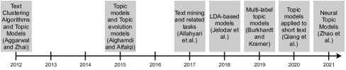
Figure 4: Timeline of Literature Reviews about Topic Modeling and Text Clustering.

We introduce this section with Figure 4, which presents a timeline (last 10 years) with surveys about clustering and topic models. [8] introduced text clustering algorithms, including feature selection, dimension reduction, particularities of text data, distance-based algorithms (agglomerative, hierarchical, partitioning, and hybrid methods), word and phrase-based clustering (including the pattern of word frequency or phrase frequency, and the combination of word clusters and document clusters), assumptions and concepts of topic models, clustering applied to text streams and networks, and concepts of semi-supervised clustering. This work mentioned outliers in the context of temporary anomalies in clusters (e.g., online clustering), such as short-term shifts. Three years later, [14] presented a survey about topic models dividing them into “topic models” and “topic evolution models”, which are algorithms that consider a temporal evolution of topics. Their focus was on explaining each algorithm based on its characteristics, examples, and limitations. Next, the work of [16] comprised a larger spectrum of text mining tasks, including text clustering (hierarchical and distance-based), text preprocessing, topic modeling (pLSA [141] and LDA [22]), information extraction (such as named entity recognition), and text classifiers. Finally, the work addressed some text mining applications in biomedicine.

In 2018, [19] investigated LDA-based topic models from 2003 to 2016 that considered applications like medicine and political sciences. In addition, the LDA algorithms involved text and other data (e.g., image and audio). They also included available datasets and frameworks. In the following year, [38] surveyed multi-label topic models, which can also perform multi-label classification tasks. The work detailed topic models concerning sampling, online, non-parametric, and dependency methods. In addition, the paper included multi-label classification and particularities of the related topic modeling. There were presented corpora for multi-label tasks, performance metrics, and current limitations of the literature. The following review, [39], comprised topic models applied to short texts. They presented a taxonomy for the algorithms, including Dirichlet multinomial mixture, global word co-occurrences, and self-aggregation. The work also provided an open-source tool (STTM) implemented in Java within a single interface. Finally, [34] shed light on neural topic models (NTMs), which emerged as competitive algorithms in the context of deep learning and NTMs challenge probabilistic topic models (e.g., LDA). The survey also provided a taxonomy for NTMs (e.g., NTMs with meta-data, NTMs for short text, sequential NTMs, NTMs with pre-trained models, NTMs based on autoregressive models, NTMs based on Generative Adversarial Nets, and NTMs based on Graph Neural Networks). Besides, the evaluation methods, limitations of NTMs, and future directions were discussed. Lastly, our work is distinct from the ones mentioned above due to its time frame and foci: reproducibility and distortion issues from initialization and outlier detection concerning text clustering and topic modeling.

9 Declaration of interests

The authors declare that they have no known competing financial interests or personal relationships that could have appeared to influence the work reported in this paper.

Appendix A Core Concept: Text Vectorization

NLP problems, which include topic modeling, typically require embedding text data into numeric vectors. This enables algebraic data manipulation necessary to fit into well-known optimization frameworks. Statistical-based (A.1), shallow neural-based (A.2), and attention neural-based (A.3) methods are presented in this section.

A.1 Statistical-Based Methods

Statistical embeddings represent every document based on term distributions and other statistics extracted from the corpus.

In the Bag-of-words (BOW), each document is represented by its word distribution. More formally, the document, comprising words from a vocabulary $V$, is transformed into a word frequency vector $d\in\mathbb{R}_{+}^{\lvert V\lvert}$. Major drawbacks of this embedding representation are high representational sparsity even in mildly sized corpora and loss of information regarding word order, hence ignoring word semantics based on the context in which they were originally inserted.

This simple idea can easily be further generalized to a Bag-of-$n$-grams, where each term becomes a sequence $n$ consecutive words (where word order matters) [94, 53, 47]. Increasing $n$ captures more relations between words and relieves the semantic loss from the original BOW, but at the expense of a higher dimensional representation with increased sparsity. Bag-of-$n$-grams can also be defined in character level instead of word level [41], essentially becoming bag-of-subwords. A total of 11 (19%) reviewed works used BOW or Bag-of-$n$-grams during their experiments.

Another popular representation is the Term Frequency-Inverse Document Frequency (TF-IDF) [82, 83, 84], which is directly proportional to the term frequency within each document and inversely proportional on a logarithm scale to how often a term appears among all the documents in the corpora. Since the precise definition for either TF or IDF terms varies in the literature, a particular formulation for TF-IDF score is shown in Equation 14.

$$\operatorname{score_{tf-idf}}(w,d;f,D,p)=\underbrace{\frac{f_{(w,d)}}{\left(\sum_{z\in d}f_{(z,d)}^{\;p}\right)^{\frac{1}{p}}}}_{\operatorname{TF}(w,\ d;\ f,p)}\cdot\underbrace{\vphantom{\frac{1}{\left(\sum f_{(z,d)}^{\;p}\right)^{\frac{1}{p}}}}\left[1-\log\left(\frac{n(w;D)+1}{\lvert D\lvert+1}\right)\right]}_{\operatorname{IDF}(w;\ D)}$$ (14)

In this equation, $D$ is the set of all documents in the corpus, $w$ is a particular term in vocabulary $V$, $d$ is a particular document in $D$, $f\in\mathbb{R}_{+}^{\lvert V\lvert\times\lvert D\lvert}$ is the frequency matrix for every term-document pair, $p>0$ defines the normalization type to the term frequency component (typically $p=1$ or $p=2$ for $\ell_{1}$ and $\ell_{2}$ normalization respectively), and $n:V\rightarrow\mathbb{N}$ maps every word $w$ to the count of documents where it appears at least once, as shown in Equation 15, where $\operatorname{\mathbb{I}}$ is an indicator function.

$$n(w;D)=\sum_{d\in D}\operatorname{\mathbb{I}}\{w\in d\}$$ (15)

A commonly used implementation of such embedding is available in the scikit-learn library [118, 119], which closely follows the definition in Equation 14 given its default parameters, with the single difference being a final document score normalization, as shown in Equation 16 with $p=2$.

$$\operatorname{score_{tf-idf}}_{\text{scikit}}(w,d;f,D,p)=\frac{\operatorname{score_{tf-idf}}(w,d;f,D,p)}{\left(\sum_{z\in d}\operatorname{score_{tf-idf}}(z,d;f,D,p)^{p}\right)^{\frac{1}{p}}}$$ (16)

The rationale behind this definition (and many other similar ones in the literature) is that terms that frequently occur in a document $d$ and are rarer in other documents are good representatives of $d$. A total of 17 (30%) reviewed works used TF-IDF as the embedding representation, making it the most popular one among the reviewed works.

A.2 Shallow Neural-Based Methods

Neural-based methods benefit from using neural networks to learn the representation of text data as dense vectors, also known as distributed representations [142], which capture semantic and syntactic properties and relationships between objects from similarity scores. These types of embeddings are also often pre-trained in large, general-purpose corpora and made publicly available. Pre-trained embeddings are widely used in topic modeling. Another advantage of neural-based embeddings is that their dimensionality is generally much smaller than traditional BOW or TF-IDF embeddings, which helps with the dimensionality issues in data clustering and factorization and also reduces representational sparsity.

The self-supervised framework word2vec [86] and [85] uses shallow neural networks to create word embeddings. It is implemented by two distinct algorithms: Continuous Bag-of-Words (CBOW) and Skip-Grams. Let $C_{t}=\{w_{(t-i)}\lvert-n\leq i\leq n\land i\neq 0\}$ be the context window to the $t$-th word $w_{t}$. CBOW works by predicting $w_{t}$ from $C_{t}$ as input, while the Skip-Grams predict $C_{t}$ from $w_{t}$ as input. This last approach is often implemented as multiple independent binary classification problems, where the model learns to decide whether words are part of $C_{t}$ or part of a randomly sampled subset of words $N_{t}$ unrelated to $w_{t}$. This approach is called Skip-Grams with Negative Sampling [86], and its objective function is shown in Equation 17. It is mathematically related to the Pointwise Mutual Information matrix [143]. From the reviewed works, 9 (16%) used word2vec as the embedding method during the experiments.

$$J(w;D)=\sum_{w_{t}\in D}\left[\sum_{w_{j}\in C_{t}}\log(1+\exp(-w_{t}^{T}w_{j}))+\sum_{w_{j}\in N_{t}}\log(1+\exp(w_{t}^{T}w_{j}))\right]$$ (17)

By observing that the co-occurrence matrix of words in $V$ is very sparse, GloVe (Global Vectors) [87] incorporates co-occurrence statistics directly into its objective function, shown in Equation 18, where $X_{(i,j)}$ is the count of co-occurrences for words $w_{i}$ and $w_{j}$ within the same context windows. While the original work claims this modification makes GloVe computationally cheaper to train and outperform word2vec in certain tasks, conclusions from [144] are the opposite when both algorithms receive proper hyperparameter tuning or are used in huge corpora. From the reviewed works, 5 (9%) used GloVe as the embedding method in its experiments.

$$J(w,b;X)=\sum_{i,j=1}^{\lvert V\lvert}\min\Bigl{(}1,\Bigl{(}\frac{X_{(i,j)}}{100}\Bigr{)}^{0.75}\Bigr{)}\left(w_{i}^{T}w_{j}+b_{i}+b{j}-\log X_{(i,j)}\right)^{2}$$ (18)

So far, the previous methods assigned a single vector to each word, which is difficult to learn good embedding for rare words, cannot generalize to out-of-vocabulary words, and do not leverage shared morphemes across words (e.g., affixes). Thus, fastText [91, 92, 93] addresses these issues by learning embeddings for subwords defined as $n$-grams of individual characters and then representing a whole word by summing up the embeddings of every piece that composes it. fastText is trained using the word2vec (Skip-Grams) framework. Only 2 (4%) works used fastText as their embedding method during the experiments. All of the aforementioned embedding methods do not address polysemy, where a single word can have very distinct meanings depending on its context.

Aiming to embed the entire documents instead of single tokens, doc2vec [88] was developed based on the word2vec idea. This framework can also be implemented with two distinct algorithms: Distributed Memory Model of Paragraph Vectors (PV-DM) and Distributed Bag-of-Words version of Paragraph Vector (PV-DBOW), which are analogous to CBOW and Skip-Grams, respectively. The main difference between this method and its word counterpart is that doc2vec also trains unique embeddings to every document, called paragraph vectors, alongside the usual word embeddings which are shared across all documents. All learned parameters are fixed after training, but paragraph vectors for unseen documents must be learned using gradient descent, which can lead to relatively high inference costs. From the reviewed works, 3 (5%) used doc2vec in their experiments.

A.3 Attention Neural-Based Methods

In the field of NLP, the concept of attention in machine learning emerged in [145] for sequence-to-sequence (seq2seq) alignment models, having captured much research interest, and therefore was developed in many nuances and now is applied to multiple tasks [146, 147]. One of the simplest and most popular variants is the scaled dot-product (or QKV) attention as shown in Equation 19, correlating every pair of tokens from the input sequences. In that setting, $Q\in\mathbb{R}^{N\times E}$ and $K,V\in\mathbb{R}^{M\times E}$, where $N$ is the length of the first input sequence, $M$ is the length of the second input sequence, and $E$ is the embedding dimension for both. The Softmax activation is taken independently for each row of its argument, thus building a probabilistic distribution for each input token from the first sentence by taking into account every token from the second sentence.

$$\operatorname{\text{att}}(Q,K,V)=\operatorname{softmax}\left(\frac{QK^{T}}{\sqrt{E}}\right)V$$ (19)

Heavily based on the machine attention concept, Transformers [148] were introduced, rapidly turning into the state-of-the-art algorithm for seq2seq processing. Their encoder-decoder neural network architecture comprises identical stacked blocks with built-in attention mechanisms and non-linear activation. With them, the concept of multi-headed Attention was also introduced, shown in Equation 20 where $h$ is the number of attention heads, $W_{i}^{Q},W_{i}^{K},W_{i}^{V}\in\mathbb{R}^{E\times(E/h)}$ for $i=1,\ldots,h$, and $W_{O}\in\mathbb{R}^{E\times E}$. Each head learns to match distinct features from the input distribution and, later, linearly combined by $W_{O}$ to form each transformer block output.

$${\operatorname{\text{MultiheadedAtt}}(Q,K,V;W)=\left[\operatorname{\text{att}}(QW_{1}^{Q},KW_{1}^{K},VW_{1}^{V}),\,\dots,\,\operatorname{\text{att}}(QW_{h}^{Q},KW_{h}^{K},VW_{h}^{V})\right]\cdot W_{O}}$$ (20)

Transformers relieved the problem of processing large chunks of text of previous seq2seq models since they process every token in parallel. However, that characteristic lacks word order information. Thus, initial transformer embeddings are combined with positional embeddings, which uniquely identify each token position. Finally, due to the chosen attention mechanism, every token embedding is built by using global information from the entire input. By combining all described characteristics, transformers are able to create embeddings that actually take into account how and where tokens are inserted into the sentences, which is why they are called contextual embeddings.

Equation 21 summarizes all described embedding characteristics, where $f$ is a function that combines both token and positional embeddings and typically consists of an addition operation. One advantage of contextual embeddings is that they can better represent polysemous words, characteristic that previously presented embedding algorithms fail to address.

$$e_{\text{contextual}}(w,d;f)=f(e_{\text{token}}(w,d),e_{\text{positional}}(\text{index}(w,d)))$$ (21)

The ubiquitous Bidirectional Encoder Representations from Transformers (BERT) [106] is a encoder-only transformer pretrained on a general-purpose English corpus (BooksCorpus [149] and the English Wikipedia) simultaneously in two self-supervised surrogate tasks, Masked Language Modeling (MLM) and Next Sentence Prediction (NSP), and made publicly available as 12-layers (base size) or 24-layers (large size) models. Currently, it is the most popular attention-based architecture for transfer learning in the field of natural language processing, being fine-tuned to many downstream tasks. BERT assumes the input sequence is tokenized as sub-word representations from WordPiece algorithm [150], thus creating embeddings for such tokens and not for individual words.

Let $T_{\text{BERT}}(\ \cdot\ ;\theta)$ be a BERT model with trainable weights $\theta$. Its output can be used as token-wise embeddings for document $d$, $T_{\text{BERT}}(d;\theta)=[e_{0},\ e_{1},\ldots,e_{\lvert d\lvert}]\in\mathbb{R}^{E\times(1+\lvert d\lvert)}$, where $\lvert d\lvert$ is the sub-word count for document $d$ and $e_{0}$ consists of the embedding corresponding to the NSP output. For a fixed-sized document representation $e\in\mathbb{R}^{E\times 1}$ one can, for instance, take the element-wise average of sub-word embeddings (discarding the NSP embedding $e_{0}$), also known as “average pooling operation”, as shown in Equation 22. Another way is to adopt $e_{0}$ as the document embedding.

$$e=\frac{1}{\lvert d\lvert}\sum_{i=1}^{\lvert d\lvert}e_{i}$$ (22)

Although one can use $T_{\text{BERT}}(d;\theta)$ directly for downstream tasks, the output from transformer encoder final blocks are often specialized to the pretraining task output space and may perform poorly on unrelated downstream tasks without any fine-tuning [151]. The output from one or a linear combination of multiple intermediary blocks tends to encode more general language features [152, 151], and thus are more appropriate to unrelated downstream tasks. For similarity-related tasks, very typical in the context of topic modeling, original BERT embeddings are remarkably unsuccessful, even worse than averaged GloVe embeddings [153].

Using transfer learning from the original pretrained BERT model, Sentence-BERT (SBERT) [153] proposes a training procedure to create models specialized in capturing similarity relationships between sentences (or small documents). This algorithm optimizes a siamese network architecture in a surrogate supervised classification task of Natural Language Inference (NLI), with 1 million sentence pairs manually annotated as contradiction, entailment or neutral (Stanford Natural Language Inference [154] and Multi-Genre NLI Corpus [155]). The objective function adopted is the cross-entropy loss as shown in Equation 23, where $T_{\text{SBERT}}(\,\cdot\,;\theta)$ is a SBERT model with trainable parameters $\theta$, $(d_{(i,a)},d_{(i,b)})$ is the $i$-th document pair from a paired (or parallel) corpora $D$, $y\in\{0,1\}^{\lvert D\lvert\times 3}$ are the one-hot encoded labels from NLI classes, and $\phi\in\mathbb{R}^{3\times 3E}$ are learnable parameters used to mix and project the document pair embeddings onto the NLI task output space and discarded after training. The logarithm and absolute value functions are applied element-wise.

$$J(\theta,\phi;D,y,T_{\text{SBERT}})=-\displaystyle\sum_{i=1}^{\lvert D\lvert}y_{(i)}\cdot\log\Bigl{(}\underbrace{\hat{y}(\overbrace{T_{\text{SBERT}}(d_{(i,a)};\theta)}^{\text{$e_{a}$: $d_{a}$ embedding}},\overbrace{T_{\text{SBERT}}(d_{(i,b)};\theta)}^{\text{$e_{b}$: $d_{b}$ embedding}};\phi)}_{\hat{y}(e_{a},\ e_{b};\ \phi)\ =\ \operatorname{softmax}\left(\phi\cdot[e_{a},\ e_{b},\ \lvert e_{a}\ -\ e_{b}\lvert]\right)}\Bigr{)}$$ (23)

To transform every piece of text $d$ into a fixed-length embedding $e_{d}$, an average pooling layer is attached to the end of SBERT (see Equation 22). Unlike the original BERT embeddings, SBERT embeddings are appropriate for similarity-based tasks such as document clustering and outlier detection. Section 6 reviewed end-to-end topic models with pre-trained transformer encoders.

Appendix B Fundamentals of Factorization Algorithms

Matrix factorization can be employed as a direct topic modeling algorithm. In addition, it can be used as a dimensionality reduction algorithm in a data processing pipeline to overcome the curse of dimensionality, which is often present in text embedding methods. This appendix presents Latent Semantic Analysis (LSA) in B.1, Non-negative Matrix Factorization (NMF) in B.2, and Latent Dirichlet Allocation (LDA) in B.3.

B.1 Latent Semantic Analysis (LSA)

Also known as Latent Semantic Indexing (LSI) [156], LSA is a simple factorization algorithm where the embedded corpus $D$, traditionally by BOW or TF-IDF (Equation 14), is factorized by Singular Value Decomposition (SVD) as shown in Equation 24, where $r=\text{rank}(D)$ denotes the number of independent features in the embedding of $D$, $U\in\mathbb{R}^{n\times r}$ denotes an orthonormal document-topic matrix, $\Sigma\in\mathbb{R}_{+}^{r\times r}$ is a non-negative diagonal matrix and by convention $\sigma_{1}\geq\dots\geq\sigma_{r}$, and $V\in\mathbb{R}^{m\times r}$ is an orthonormal feature-topic matrix.

$$\overset{D_{(n,m)}}{\underbrace{\left[\begin{array}[]{ c }\rule[2.15277pt]{34.44434pt}{0.5pt}\ d_{1}\ \rule[2.15277pt]{34.44434pt}{0.5pt}\\ \vdots\\ \rule[2.15277pt]{34.44434pt}{0.5pt}\ d_{n}\ \rule[2.15277pt]{34.44434pt}{0.5pt}\\ \end{array}\right]}_{\begin{subarray}{c}\text{Document-feature matrix:}\\ \text{Original document embeddings}\end{subarray}}}\hskip 7.11317pt=\overset{U_{(n,r)}}{\underbrace{\left[\begin{array}[]{ c }\rule[2.15277pt]{4.30554pt}{1.0pt}\ d_{1}^{{}^{\prime}}\ \rule[2.15277pt]{4.30554pt}{1.0pt}\\ \vdots\\ \rule[2.15277pt]{4.30554pt}{1.0pt}\ d_{n}^{{}^{\prime}}\ \rule[2.15277pt]{4.30554pt}{1.0pt}\\ \end{array}\right]}_{\begin{subarray}{c}\text{Document-topic matrix:}\\ \text{Documents embedded}\\ \text{in topic subspace}\end{subarray}}}\cdot\hskip 7.11317pt\overset{\Sigma_{(r,r)}}{\underbrace{\vphantom{\left[\begin{array}[]{ c }\rule[2.15277pt]{4.30554pt}{1.0pt}\ d_{1}^{{}^{\prime}}\ \rule[2.15277pt]{4.30554pt}{1.0pt}\\ \vdots\\ \rule[2.15277pt]{4.30554pt}{1.0pt}\ d_{n}^{{}^{\prime}}\ \rule[2.15277pt]{4.30554pt}{1.0pt}\\ \end{array}\right]}\left[\begin{array}[]{c c c}\sigma_{1}&&\\ &\ddots&\\ &&\sigma_{r}\\ \end{array}\right]}_{\begin{subarray}{c}\text{Topic relevance matrix:}\\ \text{Describes how important}\\ \text{every topic is}\end{subarray}}}\hskip 5.69046pt\cdot\overset{V_{(r,m)}^{T}}{\underbrace{\vphantom{\left[\begin{array}[]{ c }\rule[2.15277pt]{4.30554pt}{1.0pt}\ d_{1}^{{}^{\prime}}\ \rule[2.15277pt]{4.30554pt}{1.0pt}\\ \vdots\\ \rule[2.15277pt]{4.30554pt}{1.0pt}\ d_{n}^{{}^{\prime}}\ \rule[2.15277pt]{4.30554pt}{1.0pt}\\ \end{array}\right]}\left[\begin{array}[]{c c c}\rule[-1.07639pt]{0.5pt}{8.61108pt}&&\rule[-1.07639pt]{0.5pt}{8.61108pt}\\ v_{1}&\cdots&v_{m}\\ \rule[-1.07639pt]{0.5pt}{8.61108pt}&&\rule[-1.07639pt]{0.5pt}{8.61108pt}\\ \end{array}\right]}_{\begin{subarray}{c}\text{Topic-feature matrix:}\\ \text{maps documents}\\ \text{to topic subspace}\end{subarray}}}$$ (24)

The SVD decomposition can always be performed to any matrix $D$ and is unique up to permutations and signals. We can choose any number of topics $k$ as long as $1\leq k\leq r$ holds. If $k<r$, then Equation 24 becomes a rank-$k$ approximation to $D$ with the least Frobenius-norm error [157].

From a geometrical standpoint, the columns in $U$ compose an orthonormal vector basis of the embedding space of $D$ (when $k=r$). Thus, $U$ can represent documents in a potentially compressed embedding that spans the topic subspace, removing all the redundancy present in the original embedding. The matrix $V$ describes the linear transformation that maps $D$ into the topic subspace, $D\xrightarrow{V}U$, and $\Sigma$ keeps $U$ orthonormal, absorbing the variability inherently to each feature in the original embedding so that topics with a high corresponding $\sigma_{i}$ encode more corpus information and thus can describe documents better. When $k<r$, we approximate this relationship by only keeping the top-$k$ most relevant topics.

This formulation can be generalized by using $\Sigma^{p}$, for some sharpness hyperparameter $p\in\mathbb{R}$, controlling the relative importance of principal components (topics) [158, 144]. In fact, representing $D$ in the topic space as $U\Sigma$ or just $U$ is a matter of setting $p=1$ or $p=0$, respectively. Larger $p$ emphasizes more discriminative topics, while $p\rightarrow 0$ dilutes the relevance across topics. This hyperparameter requires tuning, but $p\rightarrow 0$ performs better in word similarity tasks [144].

The Probabilistic LSA/LSI (pLSA/pLSI) [141] is a further development from the LSA, posing the problem as to describe corpus $D$ with a probabilistic algorithm. Its objective function is shown in Equation 25 as the negative log-likelihood of $D$, where $f\in\mathbb{R}^{\lvert V\lvert\times\lvert D\lvert}$ denotes the term-document matrix of corpora $D$ with vocabulary $V$, and $z$ is a set of unknown topics such that $\lvert z\lvert$ (the number of topics) is given and fixed. The trainable model parameters are $\theta$ and $\phi$.

$$J(\theta,\phi;D,f)=-\log p\left(D;\theta,\phi,f\right)=-\sum_{d\in D}\sum_{w\in d}f_{(w,d)}\log\left(\sum_{z}p(w\lvert z;\phi_{(z,w)})p(z\lvert d;\theta_{(z,d)})\right)$$ (25)

This model has a few clear drawbacks. Firstly, the model parameter count $\lvert\theta\lvert$ grows linearly with corpus size $\lvert D\lvert$, $\lvert\theta\lvert$ $\in\mathcal{O}(\lvert D\lvert)$, making the algorithm infeasible for large corpora and raising concerns of parameter overfitting to the data [22]. The reviewed work [28] proposes a regularization strategy for pLSA. Moreover, unseen documents outside $D$ are not modeled by pLSA. From the reviewed works, 3 (5%) used LSA/LSI in their experiments, and 2 (4%) used pLSA/pLSI.

B.2 Non-negative Matrix Factorization (NMF)

The objective of NMF [89, 90] is approximating a non-negative matrix $D\in\mathbb{R}_{+}^{nxm}$ by two lower rank non-negative matrices $W\in\mathbb{R}_{+}^{nxk}$ and $H\in\mathbb{R}_{+}^{kxm}$, where $k<m$ is a hyperparameter that controls the trade-off between representation precision and computational cost. In the context of topic modeling, $D$ is the embedded corpus by non-negative features, and $k$ is the predefined number of latent topics in $D$. NMF is not unique in general and, therefore, is affected by the initial conditions [67, 58]. It is typically done by minimizing the constrained objective function expressed by Equation 26, where $\|\cdot\|_{F}$ denotes the Frobenius matrix norm. The Kullback-Leibler Divergence [159] may also be used [67].

$$\begin{split}\min\limits_{W,H}J(W,H;D)&=\min\limits_{W,H}\|D-WH\|_{F}^{2}\end{split}$$ (26)

subject to $$\quad W,H\geq 0$$

There are several algorithms to find good solution candidates [160], such as projected gradient descent [161, 162], coordinate descent [163], or scaled gradient descent as shown in Equation 27, where $\theta\in\mathbb{R}^{n\times m}$ are trainable parameters, $\eta\in\mathbb{R}_{+}^{n\times m}$ are element-wise learning rates and $\odot$ denotes matrix element-wise (or Hadamard) product.

$$\theta^{(t+1)}=\theta^{(t)}-\eta\odot\nabla_{\theta^{(t)}}J(\theta^{(t)})$$ (27)

One scaled gradient descent particular formulation to find candidate solutions for NMF is known as the Multiplicative Update (MU) [164], where particular element-wise learning rates $\eta$ are chosen and plugged into Equation 27, which guarantee that both $W$ and $H$ stay non-negative after every update. The MU rules are shown in Equation 28, where divisions are also element-wise. Although simple to present and implement, this approach has a slow convergence rate, and more sophisticated algorithms should be preferred [165, 160].

$$W_{\text{new}}=W\odot\frac{DH^{T}}{WHH^{T}}\qquad\qquad H_{\text{new}}=H\odot\frac{W^{T}D}{W^{T}WH}$$ (28)

From the perspective of topic modeling, NMF learns how to build compact representations of each document (matrix $W$) as specific mixtures (given by matrix $H$) of a predetermined number of topics ($k$), as depicted in Equation 29.

$$\overset{D_{(n,m)}}{\underbrace{\left[\begin{array}[]{ c }\rule[2.15277pt]{34.44434pt}{0.5pt}\ d_{1}\ \rule[2.15277pt]{34.44434pt}{0.5pt}\\ \vdots\\ \rule[2.15277pt]{34.44434pt}{0.5pt}\ d_{n}\ \rule[2.15277pt]{34.44434pt}{0.5pt}\\ \end{array}\right]}_{\begin{subarray}{c}\text{Document-feature matrix:}\\ \text{Original document embeddings}\end{subarray}}}\hskip 7.11317pt=\overset{W_{(n,k)}}{\underbrace{\left[\begin{array}[]{ c }\rule[2.15277pt]{4.30554pt}{1.0pt}\ d_{1}^{{}^{\prime}}\ \rule[2.15277pt]{4.30554pt}{1.0pt}\\ \vdots\\ \rule[2.15277pt]{4.30554pt}{1.0pt}\ d_{n}^{{}^{\prime}}\ \rule[2.15277pt]{4.30554pt}{1.0pt}\\ \end{array}\right]}_{\begin{subarray}{c}\text{Document-topic matrix:}\\ \text{Documents embedded}\\ \text{in topic subspace}\end{subarray}}}\cdot\hskip 7.11317pt\overset{H_{(k,m)}}{\underbrace{\vphantom{\left[\begin{array}[]{ c }\rule[2.15277pt]{4.30554pt}{1.0pt}\ d_{1}^{{}^{\prime}}\ \rule[2.15277pt]{4.30554pt}{1.0pt}\\ \vdots\\ \rule[2.15277pt]{4.30554pt}{1.0pt}\ d_{n}^{{}^{\prime}}\ \rule[2.15277pt]{4.30554pt}{1.0pt}\\ \end{array}\right]}\left[\begin{array}[]{c c c}\rule[-1.07639pt]{0.5pt}{8.61108pt}&&\rule[-1.07639pt]{0.5pt}{8.61108pt}\\ h_{1}&\cdots&h_{m}\\ \rule[-1.07639pt]{0.5pt}{8.61108pt}&&\rule[-1.07639pt]{0.5pt}{8.61108pt}\\ \end{array}\right]}_{\begin{subarray}{c}\text{Topic-feature matrix:}\\ \text{$m$ parallel learned}\\ \text{topic mixtures}\end{subarray}}}$$ (29)

The interpretation of NMF results may be non-trivial to topic modeling since NMF alone does not develop the concrete meaning for each topic, demanding further analysis of a data domain expert. Moreover, $k$ could be chosen inappropriately by overestimating or underestimating the “true” topic number, hence reducing topic coherence.

B.3 Latent Dirichlet Allocation (LDA)

LDA [22] describes a probabilistic generative algorithm by a hierarchical bayesian model, where documents are modeled as topic mixtures, and topics are modeled as word mixtures. One common description of LDA is as follows:

1. Let $D$ be text corpora with a vocabulary $V$. Choose and fix the number of topics $k$ and the desired generated document length $N$;

2. Choose and fix the hyperparameters $\alpha\in\mathbb{R}^{k}$ and $\beta\in\mathbb{R}^{V}$. Typically both vectors are chosen to have all entries with the same value (which leads to symmetric Dirichlet distributions and thus balance between topics/words) and strictly less than 1 (which leads to sparse Dirichlet distributions, corresponding to more homogeneous generated documents);

3. Sample $\theta_{i}\sim\operatorname{Dirichlet}(\alpha)$, where $i=1,\ldots,\lvert D\lvert$;

4. Sample $\phi_{j}\sim\operatorname{Dirichlet}(\beta)$, where $j=1,\dots,k$;

5. Repeat for every $i=1,\dots,\lvert D\lvert$ and $j=1,\dots,N$:

   1. Sample a topic $z_{(i,j)}\sim\operatorname{Multinomial}(\theta_{i})$;

   2. Given the chosen topic $z_{(i,j)}$, sample a word $w_{(i,j)}\sim\operatorname{Multinomial}(\phi_{z_{(i,j)}})$.

LDA makes the “bag-of-words” (or “exchangeability of words”) assumption, and, therefore, word order is not considered. It is a further generalization of pLSA/pLSI (see the objective function in Equation 25), describing a document-generation process even to unseen documents, unlike its predecessor, and also does not grow its parameter count linearly with corpus size. Its objective function is formally described by Equation 30 as the corpus negative log-likelihood, although it is intractable to compute. Thus, various algorithms were employed to approximate a solution, such as variational expectation-maximization [22], Gibbs sampling [166], and online variational bayes [167] that scales for large corpora by using mini-batch gradient descent.

$$\centering J(\alpha,\beta;D)=-\log p\left(D;\alpha,\beta\right)=-\sum_{i=1}^{\lvert D\lvert}\log\int p\left(\theta_{i};\alpha\right)\left(\prod_{j=1}^{N}\sum_{z_{(i,j)}}p(z_{(i,j)};\theta_{i})p(w_{(i,j)}\lvert z_{(i,j)};\beta)\right)d\theta_{i}\@add@centering$$ (30)

The behavior of a $\operatorname{Dirichlet}(\alpha)$ distribution for topic sampling among 3 possible options is illustrated in Figure 5. From that Dirichlet distribution (represented by the contour lines within the 2-simplex), $\theta_{i}$ parameters for multinomial distributions are drawn, which in turn define a particular distribution of topics. This process is analogous for word sampling, by using the $\operatorname{Dirichlet}(\beta)$ distribution.

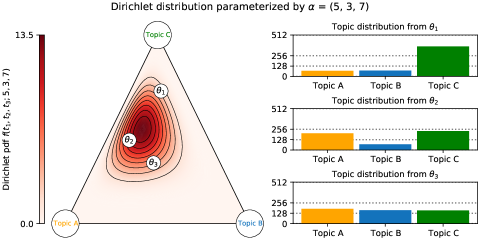
Figure 5: Example of a Dirichlet distribution for $\alpha=(5,3,7)$. Each topic is represented by a corner of a 2-simplex. Three multinomial distribution parameters $\theta_{i}$ were drawn randomly from this Dirichlet distribution and plotted in the contour plot to the left. Then, for each multinomial distribution parameterized by $\theta_{i}$, 512 samples were drawn randomly and their frequencies plotted as the bar plots to the right.

One LDA limitation is that it implicitly assumes independence between topics, which may not be reasonable in some applications. To fix this issue, slightly modified algorithms can be employed in place of LDA such as Correlated Topic Models (CTM) [18], where the topic Dirichlet distribution is replaced by a logistic Gaussian distribution (the topic multinomial distribution is parameterized by softmaxed samples from a multivariate Gaussian distribution), hence also modeling the correlation between topics in the Gaussian covariance matrix. Note that this extra representational capability does not necessarily correlate positively with human intuition for coherent topics [17]. Other LDA variants are reviewed in [19].

Similar to the NMF approach, LDA also takes for granted the number of topics $k$, and the interpretation of its results may be non-trivial since the exact meaning for each topic needs to be defined by a data domain expert. From the reviewed works, 6 (11%) used LDA as a topic modeling algorithm, and 5 (9%) used LDA to produce intermediary representations in more sophisticated pipelines.

Appendix C Core Concepts of Clustering Algorithms

Topic modeling often relies on clustering algorithms to group similar document embeddings into the same clusters, which are interpreted as topics. Despite the fact that the meaning for a “cluster” is not always clear [10, 11], current unsupervised topic modeling has shown to be able to handle natural language text data that frequently matches some of our human intuition about how the data should be grouped (and how it should not). This section presents popular clustering algorithms among the reviewed works, summarized in Table 6.

We also included each algorithm asymptotic time complexity, an important factor to consider while designing computationally scalable topic modeling pipeline. Our asymptotic notation follows set-theoretic definitions from [168], hence $f(n)\in\mathcal{O}(n)$ denoting the conventional $f(n)=\mathcal{O}(n)$ for a function $f$, and $\mathcal{O}(f(n))\subseteq\mathcal{O}(g(n))$ denoting $\mathcal{O}(f(n))\leq\mathcal{O}(g(n))$ for some $f(n)\in\mathcal{O}(g(n))$. The embedding dimension is omitted from the asymptotic analysis for simplicity, but it is worth noting that compact representations also improves running time, as distance or similarity computations are necessary to group instances.

Table 6: Taxonomy of reviewed clustering algorithms in this present work.

	Flat clusters	Hierarchical clusters
Representative-based	K-means	HAC (single-linkage)
	Spherical K-means	HAC (complete-linkage)
	Fuzzy K-means	HAC (group average-linkage)
	K-medoids (PAM/FasterPAM)	HAC (Ward’s method)
	CLARA/FasterCLARA
	CLARANS/FasterCLARANS
Density-based	DBSCAN	HDBSCAN

This appendix is divided as follows: representative-based clustering (C.1), hierarchical clustering (C.2), density-based clustering (C.3), and the connection with factorization algorithms (C.4).

C.1 Representative-Based Clustering

Algorithms within this class compute similarity scores (or distances) between instances to build a representative object for each cluster. Equivalently, every document is represented by a similar representative object or by a weighted average of representatives proportional to the degree of similarity.

K-means [169] is the most popular clustering algorithm among the reviewed works (17 (30%) total works), used as part of the topic modeling pipeline or a baseline algorithm for more sophisticated ones. It is a partitioning algorithm, hence attributing each document to precisely one cluster. Two key assumptions of this algorithm are that the maximum number of clusters or topics $k$ is known and fixed in advance (which is not necessarily a reasonable assumption), and each topic follows a distribution with equal variance in every dimension. Geometrically, it means that topics should, presumably, be modeled as hyperspherical document clouds with the same radii.

Formally, the k-means algorithm minimizes the objective function shown in Equation 31, the sum of squared Euclidean distances between every embedded document $d$ and its cluster center of mass $\mu\in C$, known as centroid or cluster prototype, with $C\in\mathbb{R}^{k\times\lvert d\lvert}$. Note that this objective function is not equivalent to minimizing the Euclidean distances between the documents and their cluster centers, which consists of a different and harder problem known as the Fermat-Weber Problem [170]. It is, however, equivalent to minimizing cluster weighted intra-variances.

$$J(C;D)=\sum_{d\in D}\min\limits_{\mu\in C}\|d-\mu\|_{2}^{2}$$ (31)

Since finding the global minimum of this objective function is NP-hard [171, 172], heuristics are employed to find local minima, often posed as coordinate ascent algorithms such as the Lloyd’s Algorithm [173] or more sophisticated and faster ones [174]. The Lloyd’s Algorithm has an exponential worst-case time complexity of $2^{\Omega(\lvert D\lvert)}$ against adversarial examples [175], but, in practice, it tends to run in linear average time complexity of $\mathcal{O}(Nk\lvert D\lvert)$, where $N$ is the maximum number of optimization steps.

A soft-clustering alternative for K-means is Fuzzy K-means [176, 177], also known as Fuzzy C-means. In this algorithm, each document is inserted into every cluster with varying degrees of membership. The corresponding objective function is shown in Equation 32, where $p\in(1,+\infty)$ is a hyperparameter that controls how fuzzy the cluster assignments tend to; as $p\rightarrow 1$, the cluster assignments will tend to be less distributed, while as $p\rightarrow+\infty$ the cluster assignments will tend to a uniform distribution. This algorithm is used by 2 (4%) reviewed works [7, 72].

$$J(C;D,k,p)=\sum_{d\in D}\sum_{j=1}^{k}\left(\left[\sum_{z=1}^{k}\left(\frac{\|d-\mu_{k}\|_{2}^{2}}{\|d-\mu_{z}\|_{2}^{2}}\right)^{\frac{1}{p-1}}\right]^{-p}\cdot\hskip 4.26773pt\|d-\mu_{k}\|_{2}^{2}\right)$$ (32)

Employing fuzzy clustering strategies have the benefit of introducing the notion of confidence to the results, since documents next to cluster boundaries will have fuzzier assignments (degrees of membership more distributed) than documents next to the cluster center of mass (with degrees of membership more concentrated on a single cluster).

To cluster documents, the cosine similarity (the cosine of the smallest angle between two embedded documents, see Equation 2) is frequently used rather than the squared Euclidean distance. To achieve this, the classical K-means needs two modifications, which are normalizing the document embeddings $d$ and each centroid estimation $\mu_{k}$ by the $\ell_{2}$-norm, $d^{\prime}=d/\|d\|_{2}$ and $\mu^{\prime}=\mu/\|\mu\|_{2}$. Such an approach is known as Spherical K-means [178] and its objective function maximizes the cosine similarity, as shown in Equation C.1. It was used by 2 (4%) reviewed works [67, 58].

$$J(C;D^{\prime},k) =\sum_{d^{\prime}\in D^{\prime}}\min\limits_{\mu^{\prime}\in C}\|d^{\prime}-\mu^{\prime}\|_{2}^{2}=\sum_{d^{\prime}\in D^{\prime}}\min\limits_{\mu^{\prime}\in C}(d^{\prime}-\mu^{\prime})^{T}(d^{\prime}-\mu^{\prime})$$

$$=\sum_{d^{\prime}\in D^{\prime}}\min\limits_{\mu^{\prime}\in C}\left(\|d^{\prime}\|_{2}^{2}+\|\mu^{\prime}\|_{2}^{2}-2d^{\prime}{}^{T}\mu^{\prime}\right)=\sum_{d^{\prime}\in D^{\prime}}\min\limits_{\mu^{\prime}\in C}\left(2-2\cos(d^{\prime},\mu^{\prime})\right)$$ (33)

$$=\sum_{d^{\prime}\in D^{\prime}}\max\limits_{\mu^{\prime}\in C}\cos(d^{\prime},\mu^{\prime})$$

One major drawback of K-means and its direct variants is that they are too sensitive to “outliers”. Since it minimizes squared distances to centroids, too distant instances greatly impact the optimal solution. The K-medoids problem also consists of data partitioning to minimize dissimilarities (not necessarily distance functions) from documents to their corresponding medoids $m$, which are necessarily existing documents in the corpus ($m\in D$). Equation 34 formalizes, mathematically, the objective function for this problem as the total negative similarity (or, analogously, the total dissimilarity) for an arbitrary similarity function which, if chosen appropriately, poses an objective function less sensitive to outliers than the traditional K-means objective (which would not be the case if the similarity chosen is the negative squared Euclidean distance, see [10]).

$$J(M;D)=-\sum_{d\in D}\max\limits_{m\in M}\operatorname{similarity}(d,m)$$ (34)

Similar to K-means, finding the optimal K-medoids solution is also an NP-hard problem. Hence, only local minima found by heuristics can be efficiently computed, the most popular being the Partition Around Medoids (PAM) algorithm, used by 4 (7%) reviewed works. Albeit robust against outliers with an appropriate similarity function, PAM is not scalable to large corpora since its time complexity is of $\mathcal{O}(Nk(\lvert D\lvert-k)^{2})\subseteq\mathcal{O}(Nk\lvert D\lvert^{2}+Nk^{3})$, a quadratic growth with respect to corpus size $\lvert D\lvert$.

Clustering LARge Applications (CLARA) [179, 180] is an algorithm that runs PAM on document subsets from corpus $S\subseteq D$, thus scaling the time complexity quadratically only to the subset size $\lvert S\lvert$ but linear growth on corpora size $\lvert D\lvert$, $\mathcal{O}(Nk(\lvert S\lvert-k)^{2}+Nk(\lvert D\lvert-k))$. The traditional recommendation is to choose $\lvert S\lvert\in\mathcal{O}(k)$ such as $\lvert S\lvert=40+2k$, and hence the time complexity becomes $\mathcal{O}(Nk^{3}+Nk\lvert D\lvert)$. Another well known PAM modification is the algorithm Clustering Large Applications based on RANdomized Search (CLARANS) [181], which adds more randomization to CLARA in order to reduce execution cost.

These algorithms have been continuously optimized since their invention. Recently, [73] proposed FasterPAM, consisting of a faster algorithm equivalent to the original PAM (and consequently proposing FasterCLARA and FasterCLARANS since they rely directly on PAM implementation), reducing time complexity of PAM optimization steps up to a factor of $\mathcal{O}(k)$ to $\mathcal{O}(N\lvert D\lvert(\lvert D\lvert-k))\subseteq\mathcal{O}(N\lvert D\lvert^{2})$, and hence $\mathcal{O}(Nk^{2})$ for FasterCLARA and FasterCLARANS (by choosing $\lvert S\lvert\in\mathcal{O}(k)$). This same work also proposes to at least double the traditional recommended sample size $\lvert S\lvert=80+4k$.

C.2 Hierarchical Clustering

From 8 (14%) works that used hierarchical clustering algorithms in their experiments, 7 employed Hierarchical Agglomerative Clustering (HAC) algorithms varying the linkage (how to define the dissimilarity of two clusters given they have multiple objects) from single, complete, group average and Ward’s method. While the linkage is a very important hyperparameter that often drastically changes the resulting cluster structure, all the cited linkages can be viewed by the Lance-Williams (LW) unified HAC mathematical framework [182] shown in Equation 35, where $S_{z}$ denotes the $z$-th partition, $S_{i}\cup S_{j}$ denotes a candidate fusion of partitions $S_{i}$ and $S_{j}$, $d:S^{2}\rightarrow\mathbb{R}$ denotes some dissimilarity measure, $\alpha:\mathbb{N}^{3}\rightarrow\mathbb{R}^{4}$ is a specific weight vector that defines a linkage method, and $n_{z}=\lvert S_{z}\lvert$ for brevity. This recurrent formula is optimized greedily by the HAC implementations.

$$\begin{split}d(S_{i}\cup S_{j},S_{k})=\left[d(S_{i},S_{k}),d(S_{j},S_{k}),d(S_{i},S_{j}),\lvert d(S_{i},S_{k})-d(S_{j},S_{k})\lvert\right]^{T}\cdot\hskip 2.84544pt\alpha(n_{i},n_{j},n_{k})\end{split}$$ (35)

While single linkage (also known as minimal or nearest neighbor linkage) is the most flexible approach to model arbitrary cluster shapes, local data variations affect the whole cluster structure, and therefore seemingly distinct clusters may end up connected very early by narrow paths in-between clusters. This last property is the chaining effect, where the single linkage is the linkage method affected by it the most among the cited linkages. Complete linkage (also known as maximal, clique or farthest neighbor linkage) is less affected by local variations, but is biased towards hyperspherical-like cluster shapes and tends to fragment large clusters. The (group) average linkage is a compromise between single and complete linkage ([108, p.284], [107, p.559]). In the LW framework, $\alpha_{\text{single}}^{T}=\left[\frac{1}{2},\frac{1}{2},0,-\frac{1}{2}\right]^{T}$, $\alpha_{\text{complete}}^{T}=\left[\frac{1}{2},\frac{1}{2},0,\frac{1}{2}\right]^{T}$ and $\alpha_{\text{avg}}^{T}=\left[\frac{n_{i}}{(n_{i}+n_{j})},\frac{n_{j}}{(n_{i}+n_{j})},0,0\right]^{T}$ [182].

The traditional Ward’s linkage (also known as the Ward’s method) [183, 184] corresponds to a special case of the objective function shown in Equation 36 when $p=q=2$, where $A,B$ are candidate partitions to fusion [185]. By using this objective function, the Ward’s linkage is generalized to any value of $p\in(0,2]$ if $q=2$, which corresponds to optimizing to particular cases of Minkowski distance rather than the usual squared Euclidean distance. It is also valid for $p=q=1$, corresponding to minimizing the Manhattan (or $\ell_{1}$) distance [186]. In the LW framework, $\alpha_{\text{ward}}^{T}=\left[\frac{(n_{i}+n_{k})}{M},\frac{(n_{j}+n_{k})}{M},-\frac{n_{k}}{M},0\right]^{T}$ where $M=n_{i}+n_{j}+n_{k}$ and for every valid Ward’s linkage generalization described previously [187, 185, 186].

$$\begin{split}d(A,B;p,q)=\frac{n_{a}n_{b}}{n_{a}+n_{b}}\left(\frac{2}{n_{a}n_{b}}\sum_{i=1}^{n_{a}}\sum_{j=1}^{n_{b}}\|a_{i}-b_{j}\|_{q}^{p}-\frac{1}{n_{a}^{2}}\sum_{i,j=1}^{n_{a}}\|a_{i}-a_{j}\|_{q}^{p}-\frac{1}{n_{b}^{2}}\sum_{i,j=1}^{n_{b}}\|b_{i}-b_{j}\|_{q}^{p}\right)\end{split}$$ (36)

If naively implemented, the worst-case time complexity for every linkage listed in this section is $\mathcal{O}(\lvert D\lvert^{3})$, but it can all be further reduced to $\mathcal{O}(\lvert D\lvert^{2})$ by using more intelligent methods such as Reciprocal Nearest Neighbors Chain (see [188, 184, 189]) or simple heap-based algorithms with worst-case time complexity of $\mathcal{O}(\lvert D\lvert^{2}\log\lvert D\lvert)$ [6, 107]. Since every mentioned linkage function has the same worst-case time complexity, it must be chosen accordingly to the task at hand if quadratic running time in relation to corpus size is still acceptable.

C.3 Density-Based Clustering

Density-based Spatial Clustering of Applications with Noise (DBSCAN) [190] builds clusters for regions with a high concentration of data or densely populated. It is dependent on tuning two hyperparameters $\epsilon>0$, which are a fixed minimum radius to decide whether two points in space are considered connected, and $m\in\mathbb{N}$ that is the minimum number of connections a point $d$ needs to satisfy to be considered a core point. Core points reachable from each other (there is a connected path consisting of only core points between both) are clustered together, alongside all non-core points directly connected to at least one core point (so-called border points). Non-core and non-border points are considered outliers and are not clustered.

Three benefits of DBSCAN are its natural capacity of handling outlier documents, it does not assume the number of clusters that must be built, and it can build clusters of arbitrary shapes and volume. The downsides are its inherent dependency of hyperparameter tuning and, since they both fix a priori the rules on how the points must be connected, the algorithm cannot appropriately handle data with varying densities [191, 107, p.569]. It has a worst-case time complexity of $\mathcal{O}(\lvert D\lvert^{2})$ but only $\mathcal{O}(\lvert D\lvert\log\lvert D\lvert)$ in average. This was used in 2 (4%) reviewed work experiments [43, 42].

Hierarchical DBSCAN (HDBSCAN) [191] is a direct extension of the classical DBSCAN algorithm. As its name suggests, it combines both the density and hierarchical clustering approaches, which means it finds densely populated regions but also connects hierarchically those regions by similarity. Thus, HDBSCAN can be thought of as running DBSCAN to infinitely many $\epsilon$ parameters simultaneously. Hence, HDBSCAN does not suffer from variable density in data and is also more insensitive to its hyperparameter selection than the original DBSCAN. Its time complexity was originally $\mathcal{O}(\lvert D\lvert^{2})$ but was improved to approximately $\mathcal{O}(g(D)\lvert D\lvert\log\lvert D\lvert)$ on average by [192], where $g(D)$ represents non-trivial, data-dependent factors to the power up to 10. Nevertheless, [192] shows that HDBSCAN running time is comparable to the original DBSCAN in practice. Despite its potential, only one reviewed work used HDBSCAN [9].

C.4 Connection with Factorization Algorithms

The NMF algorithm has natural soft (or fuzzy) clustering interpretation due to the non-negativity constraints [193, 194]. More precisely, after the factorization, the matrix $W\in\mathbb{R}_{+}^{n\times k}$ can be interpreted as the membership scores of each document to every latent topic [67, 54, 55, 59]. A similar analysis can be made to LSA/LSI and pLSA/pLSI due to their connections with NMF and other clustering algorithms [195, 196]. LDA already gives a document membership score for each latent topic by design, and thus also has a soft-clustering interpretation.

Appendix D Acknowledgment

This work was supported by Brazil’s Chamber of Deputies, CAPES, CNPq (grant number: 309858/2021-6), and Google (Latin America Research Awards - first author).

References

- [1] Amir Gandomi and Murtaza Haider. Beyond the hype: Big data concepts, methods, and analytics. International Journal of Information Management, 35(2):137–144, 2015.
- [2] Domo. Data Never Sleeps 9.0, 2021. Accessed: 2021-12-28.
- [3] Daniel Jurafsky and James H Martin. Speech and language processing (draft). 2021.
- [4] Matthew J Page, Joanne E McKenzie, Patrick M Bossuyt, Isabelle Boutron, Tammy C Hoffmann, Cynthia D Mulrow, Larissa Shamseer, Jennifer M Tetzlaff, Elie A Akl, Sue E Brennan, Roger Chou, Julie Glanville, Jeremy M Grimshaw, Asbjørn Hróbjartsson, Manoj M Lalu, Tianjing Li, Elizabeth W Loder, Evan Mayo-Wilson, Steve McDonald, Luke A McGuinness, Lesley A Stewart, James Thomas, Andrea C Tricco, Vivian A Welch, Penny Whiting, and David Moher. The PRISMA 2020 statement: an updated guideline for reporting systematic reviews. BMJ, 372, 2021.
- [5] W.Z. Zhu and R.B. Allen. Document clustering using the LSI subspace signature model. Journal of the American Society for Information Science and Technology, 64:844–860, 4 2013.
- [6] Christopher D. Manning, Prabhakar Raghavan, and Hinrich Schütze. Introduction to Information Retrieval. Cambridge University Press, USA, 2008.
- [7] Murtadha Talib AL-Sharuee, Fei Liu, and Mahardhika Pratama. Sentiment analysis: An automatic contextual analysis and ensemble clustering approach and comparison. Data & Knowledge Engineering, 115:194–213, 5 2018.
- [8] Charu C. Aggarwal and ChengXiang Zhai. A Survey of Text Clustering Algorithms, pages 77–128. Springer US, Boston, MA, 2012.
- [9] Maarten Grootendorst. BERTopic: Leveraging BERT and c-TF-IDF to create easily interpretable topics., 2020.
- [10] Vladimir Estivill-Castro. Why so Many Clustering Algorithms: A Position Paper. SIGKDD Explor. Newsl., 4(1):65–75, June 2002.
- [11] Christian Hennig. What are the true clusters? Pattern Recognition Letters, 64:53–62, 2015. Philosophical Aspects of Pattern Recognition.
- [12] Ismail Harrando, Pasquale Lisena, and Raphaël Troncy. Apples to Apples: A Systematic Evaluation of Topic Models. pages 483–493, September 2021.
- [13] David M. Blei. Probabilistic Topic Models. Commun. ACM, 55(4):77–84, apr 2012.
- [14] Rubayyi Alghamdi and Khalid Alfalqi. A Survey of Topic Modeling in Text Mining. International Journal of Advanced Computer Science and Applications, 6(1), 2015.
- [15] Alexander Miserlis Hoyle, Pranav Goel, Andrew Hian-Cheong, Denis Peskov, Jordan Boyd-Graber, and Philip Resnik. Is Automated Topic Model Evaluation Broken?: The Incoherence of Coherence. In Advances in Neural Information Processing Systems, 2021.
- [16] Mehdi Allahyari, Seyedamin Pouriyeh, Mehdi Assefi, Saied Safaei, Elizabeth D. Trippe, Juan B. Gutierrez, and Krys Kochut. A Brief Survey of Text Mining: Classification, Clustering and Extraction Techniques, 2017.
- [17] Jonathan Chang, Sean Gerrish, Chong Wang, Jordan Boyd-graber, and David Blei. Reading Tea Leaves: How Humans Interpret Topic Models. In Y. Bengio, D. Schuurmans, J. Lafferty, C. Williams, and A. Culotta, editors, Advances in Neural Information Processing Systems, volume 22, pages 1–9, Vancouver, B.C., Canada., 2009. Curran Associates, Inc.
- [18] John Lafferty and David Blei. Correlated Topic Models. In Y. Weiss, B. Schölkopf, and J. Platt, editors, Advances in Neural Information Processing Systems, volume 18, Vancouver, B.C., Canada, 2006. MIT Press.
- [19] Hamed Jelodar, Yongli Wang, Chi Yuan, Xia Feng, Xiahui Jiang, Yanchao Li, and Liang Zhao. Latent Dirichlet allocation (LDA) and topic modeling: models, applications, a survey. 78(11):15169–15211, November 2018.
- [20] Amy N. Langville, Carl D. Meyer, Russell Albright, James Cox, and David Duling. Algorithms, Initializations, and Convergence for the Nonnegative Matrix Factorization, 2014.
- [21] Wathsala Anupama Mohotti and Richi Nayak. Efficient Outlier Detection in Text Corpus Using Rare Frequency and Ranking. ACM Transactions on Knowledge Discovery from Data, 14:71(1–30), 10 2020.
- [22] David M. Blei, Andrew Y. Ng, and Michael I. Jordan. Latent Dirichlet Allocation. J. Mach. Learn. Res., 3:993–1022, March 2003.
- [23] Cátia M. Salgado, Carlos Azevedo, Hugo Proença, and Susana M. Vieira. Noise Versus Outliers, pages 163–183. Springer International Publishing, Cham, 2016.
- [24] Varun Chandola. Anomaly Detection: A Survey. ACM Computing Surveys, 2009.
- [25] Hongzhi Wang, Mohamed Jaward Bah, and Mohamed Hammad. Progress in Outlier Detection Techniques: A Survey. IEEE Access, 7:107964–108000, 2019.
- [26] Charu C. Aggarwal. Outlier Analysis. Springer, New York, NY, 2013.
- [27] Ander Carreño, Iñaki Inza, and José Antonio Lozano. Analyzing rare event, anomaly, novelty and outlier detection terms under the supervised classification framework. Artificial Intelligence Review, 53:3575–3594, 2019.
- [28] Eugeniia Veselova and Konstantin Vorontsov. Topic Balancing with Additive Regularization of Topic Models. pages 59–65, 7 2020.
- [29] Erich Schubert, Michael Weiler, and Hans Peter Kriegel. SigniTrend: Scalable detection of emerging topics in textual streams by hashed significance thresholds. pages 871–880, New York, NY, USA, 8 2014. ACM.
- [30] Guilherme O Campos, Arthur Zimek, Jörg Sander, Ricardo J G B Campello, Barbora Micenková, Erich Schubert, Ira Assent, and Michael E Houle. On the evaluation of unsupervised outlier detection: measures, datasets, and an empirical study. Data Min. Knowl. Discov., 30(4):891–927, July 2016.
- [31] Lukas Ruff, Jacob R. Kauffmann, Robert A. Vandermeulen, Grégoire Montavon, Wojciech Samek, Marius Kloft, Thomas G. Dietterich, and Klaus-Robert Müller. A Unifying Review of Deep and Shallow Anomaly Detection. Proceedings of the IEEE, 109(5):756–795, 2021.
- [32] Andrew Emmott, Shubhomoy Das, Thomas Dietterich, Alan Fern, and Weng-Keen Wong. A Meta-Analysis of the Anomaly Detection Problem, 2015.
- [33] Songqiao Han, Xiyang Hu, Hailiang Huang, Mingqi Jiang, and Yue Zhao. ADBench: Anomaly Detection Benchmark, 2022.
- [34] He Zhao, Dinh Phung, Viet Huynh, Yuan Jin, Lan Du, and Wray Buntine. Topic Modelling Meets Deep Neural Networks: A Survey. In Zhi-Hua Zhou, editor, Proceedings of the Thirtieth International Joint Conference on Artificial Intelligence, IJCAI-21, pages 4713–4720, Montreal (online), 8 2021. International Joint Conferences on Artificial Intelligence Organization. Survey Track.
- [35] Silvia Terragni, Elisabetta Fersini, Bruno Giovanni Galuzzi, Pietro Tropeano, and Antonio Candelieri. OCTIS: Comparing and Optimizing Topic models is Simple! In Proceedings of the 16th Conference of the European Chapter of the Association for Computational Linguistics: System Demonstrations, pages 263–270, Online, April 2021. Association for Computational Linguistics.
- [36] Pasquale Lisena, Ismail Harrando, Oussama Kandakji, and Raphael Troncy. TOMODAPI: A Topic Modeling API to Train, Use and Compare Topic Models. In Proceedings of Second Workshop for NLP Open Source Software (NLP-OSS), pages 132–140, Online, November 2020. Association for Computational Linguistics.
- [37] Caitlin Doogan and Wray Buntine. Topic Model or Topic Twaddle? Re-evaluating Semantic Interpretability Measures. In Proceedings of the 2021 Conference of the North American Chapter of the Association for Computational Linguistics: Human Language Technologies, pages 3824–3848, Online, June 2021. Association for Computational Linguistics.
- [38] Sophie Burkhardt and Stefan Kramer. A Survey of Multi-Label Topic Models. SIGKDD Explor. Newsl., 21(2):61–79, November 2019.
- [39] Jipeng Qiang, Zhenyu Qian, Yun Li, Yunhao Yuan, and Xindong Wu. Short Text Topic Modeling Techniques, Applications, and Performance: A Survey. IEEE Transactions on Knowledge and Data Engineering, 2020.
- [40] Larissa Shamseer, David Moher, Mike Clarke, Davina Ghersi, Alessandro Liberati, Mark Petticrew, Paul Shekelle, and Lesley A Stewart. Preferred reporting items for systematic review and meta-analysis protocols (PRISMA-P) 2015: elaboration and explanation. BMJ, 349, 2015.
- [41] Deepak P. Unsupervised Separation of Transliterable and Native Words for Malayalam. In Proceedings of the 14th International Conference on Natural Language Processing (ICON-2017), pages 155–164, Kolkata, India, December 2017. NLP Association of India.
- [42] Elham Amouee, Morteza Zanjireh, Mahdi Bahaghighat, and Mohsen Ghorbani. A new anomalous text detection approach using unsupervised methods. Facta universitatis - series: Electronics and Energetics, 33:631–653, 2020.
- [43] Santipong Thaiprayoon, Herwig Unger, and Mario Kubek. Graph and Centroid-based Word Clustering. pages 163–168, New York, NY, USA, 12 2020. ACM.
- [44] Adithya Bandi, Karuna Joshi, and Varish Mulwad. Affinity Propagation Initialisation Based Proximity Clustering for Labeling in Natural Language Based Big Data Systems. Proceedings - 2020 IEEE 6th Intl Conference on Big Data Security on Cloud, BigDataSecurity 2020, 2020 IEEE Intl Conference on High Performance and Smart Computing, HPSC 2020 and 2020 IEEE Intl Conference on Intelligent Data and Security, IDS 2020, pages 1–7, 2020.
- [45] Manuel R. Ciosici, Ira Assent, and Leon Derczynski. Accelerated High-Quality Mutual-Information Based Word Clustering. In Proceedings of the 12th Language Resources and Evaluation Conference, pages 2491–2496, Marseille, France, May 2020. European Language Resources Association.
- [46] Jieun Kim and Changyong Lee. Novelty-focused weak signal detection in futuristic data: Assessing the rarity and paradigm unrelatedness of signals. Technological Forecasting and Social Change, 120:59–76, 2017.
- [47] Önder Babur. Statistical analysis of large sets of models. pages 888–891, New York, NY, USA, 8 2016. ACM.
- [48] R. Vasanth Kumar Mehta, B. Sankarasubramaniam, and S. Rajalakshmi. An algorithm for fuzzy-based sentence-level document clustering for micro-level contradiction analysis. pages 102–105, Chennai, India, 2012. Association for Computing Machinery.
- [49] Uraiwan Buatoom, Waree Kongprawechnon, and Thanaruk Theeramunkong. Document clustering using K-means with term weighting as similarity-based constraints. Symmetry, 12:1–25, 2020.
- [50] Md Rashadul Hasan Rakib, Norbert Zeh, Magdalena Jankowska, and Evangelos Milios. Enhancement of Short Text Clustering by Iterative Classification, 2020.
- [51] Xiao Pu, Nikolaos Pappas, and Andrei Popescu-Belis. Sense-Aware Statistical Machine Translation using Adaptive Context-Dependent Clustering. volume 1, pages 1–10, Copenhagen, Denmark, 1 2017. Association for Computational Linguistics (ACL).
- [52] Ali Vardasbi, Heshaam Faili, and Masoud Asadpour. Solving submodular text processing problems using influence graphs. Social Network Analysis and Mining 2019 9:1, 9:1–15, 5 2019.
- [53] Shen Li, Zhe Zhao, Tao Liu, Renfen Hu, and Xiaoyong Du. Initializing convolutional filters with semantic features for text classification. pages 1884–1889, Copenhagen, Denmark, 2017. Association for Computational Linguistics.
- [54] Kai Liu and Hua Wang. Robust multi-relational clustering via 1-Norm symmetric nonnegative matrix factorization. volume 2, pages 397–401, Beijing, China, 2015. Association for Computational Linguistics.
- [55] Gabriella Casalino, Ciro Castiello, Nicoletta Del Buono, and Corrado Mencar. Intelligent Twitter Data Analysis Based on Nonnegative Matrix Factorizations. pages 188–202, Trieste, Italy, 2017. Springer, Cham.
- [56] Aytug Onan. A K-medoids based clustering scheme with an application to document clustering. pages 354–359, Antalya, Turkey, 10 2017. IEEE.
- [57] Kansheng Shi, Lemin Li, Jie He, Haitao Liu, Naitong Zhang, and Wentao Song. A linguistic feature based text clustering method. pages 108–112, Beijing, China, 9 2011. IEEE.
- [58] Ali Hassani, Amir Iranmanesh, and Najme Mansouri. Text mining using nonnegative matrix factorization and latent semantic analysis. Neural Computing and Applications, 6, 2021.
- [59] Morten Mørup and Lars Kai Hansen. Archetypal analysis for machine learning and data mining. Neurocomputing, 80:54–63, 2012.
- [60] Renato Cordeiro De Amorim and Marcos Zampieri. Effective spell checking methods using clustering algorithms. pages 172–178, Hissar, Bulgaria, 2013. INCOMA Ltd. Shoumen, BULGARIA.
- [61] Jing Peng, Anna Feldman, and Ekaterina Vylomova. Classifying idiomatic and literal expressions using topic models and intensity of emotions. EMNLP 2014 - 2014 Conference on Empirical Methods in Natural Language Processing, Proceedings of the Conference, pages 2019–2027, 2014.
- [62] Shraey Bhatia, Jey Han Lau, and Timothy Baldwin. Topic Intrusion for Automatic Topic Model Evaluation. pages 844–849, Brussels, Belgium, 2018. Association for Computational Linguistics.
- [63] Honglei Zhuang, Chi Wang, Fangbo Tao, Lance Kaplan, and Jiawei Han. Identifying semantically deviating outlier documents. pages 2748–2757, Copenhagen, Denmark, 2017. Association for Computational Linguistics.
- [64] Xiaobing Xue and Xiaoxin Yin. Topic modeling for named entity queries. pages 2009–2012, Glasgow, Scotland, UK, 2011. ACM Press.
- [65] Rizka Wakhidatus Sholikah, Yasuhiko Morimoto, Agus Zainal Arifin, Chastine Fatichah, and Ayu Purwarianti. Exploiting comparable corpora to enhance bilingual lexicon induction from monolingual corpora. International Journal of Intelligent Engineering and Systems, 13:379–391, 2020.
- [66] Juite Wang and Yi Jing Chen. A novelty detection patent mining approach for analyzing technological opportunities. Advanced Engineering Informatics, 42:100941, 2019.
- [67] Mickael Febrissy and Mohamed Nadif. A Consensus Approach to Improve NMF Document Clustering. Lecture Notes in Computer Science (including subseries Lecture Notes in Artificial Intelligence and Lecture Notes in Bioinformatics), 12080 LNCS:171–183, 2020.
- [68] Yunsu Kim, Andreas Guta, Joern Wuebker, and Hermann Ney. A Comparative Study on Vocabulary Reduction for Phrase Table Smoothing. pages 110–117, Berlin, Germany, 2016. Association for Computational Linguistics.
- [69] Hanna Wecker, Annemarie Friedrich, and Heike Adel. ClusterDataSplit: Exploring Challenging Clustering-Based Data Splits for Model Performance Evaluation. pages 155–163, Online Conference, 11 2020. Association for Computational Linguistics (ACL).
- [70] Donatella Gubiani, Elsa Fabbretti, Bojan Cestnik, Nada Lavrač, and Tanja Urbančič. Outlier based literature exploration for cross-domain linking of Alzheimer’s disease and gut microbiota. Expert Systems with Applications, 85:386–396, 11 2017.
- [71] Deepak P. MixKMeans: Clustering Question-Answer Archives. pages 1576–1585, Austin, Texas, 2016. Association for Computational Linguistics.
- [72] Farek Lazhar. Fuzzy clustering-based semi-supervised approach for outlier detection in big text data. Progress in Artificial Intelligence, 8:123–132, 2019.
- [73] Erich Schubert and Peter J. Rousseeuw. Fast and eager k-medoids clustering: O(k) runtime improvement of the PAM, CLARA, and CLARANS algorithms. Information Systems, 101:101804, 2021.
- [74] Markus M. Breunig, Hans-Peter Kriegel, Raymond T. Ng, and Jörg Sander. LOF: Identifying Density-Based Local Outliers. SIGMOD Rec., 29(2):93–104, May 2000.
- [75] Sergio Consoli, Domenico Perrotta, and Marco Turchi. Reduced Variable Neighbourhood Search for the Generation of Controlled Circular Data. Lecture Notes in Computer Science (including subseries Lecture Notes in Artificial Intelligence and Lecture Notes in Bioinformatics), 12559 LNCS:83–98, 3 2021.
- [76] Hinrich Schütze. Integrating history-length interpolation and classes in language modeling. volume 1, pages 1516–1525, Portland, Oregon, 2011. Association for Computational Linguistics.
- [77] Seungwan Seo, Deokseong Seo, Myeongjun Jang, Jaeyun Jeong, and Pilsung Kang. Unusual customer response identification and visualization based on text mining and anomaly detection. Expert Systems with Applications, 144:1–12, 4 2020.
- [78] Tomasz Walkowiak, Szymon Datko, and Henryk Maciejewski. Distance Metrics in Open-Set Classification of Text Documents by Local Outlier Factor and Doc2Vec. In Franz Wotawa, Gerhard Friedrich, Ingo Pill, Roxane Koitz-Hristov, and Moonis Ali, editors, Advances and Trends in Artificial Intelligence. From Theory to Practice, pages 102–109, Cham, 2019. Springer International Publishing.
- [79] Ramakrishnan Kannan, Hyenkyun Woo, Charu C. Aggarwal, and Haesun Park. Outlier Detection for Text Data: An Extended Version, 2017.
- [80] José Camacho-Collados and Roberto Navigli. Find the word that does not belong: A Framework for an Intrinsic Evaluation of Word Vector Representations. pages 43–50, Stroudsburg, PA, USA, 2016. Association for Computational Linguistics.
- [81] Enrico Santus, Hongmin Wang, Emmanuele Chersoni, and Yue Zhang. A rank-based similarity metric for word embeddings. ACL 2018 - 56th Annual Meeting of the Association for Computational Linguistics, Proceedings of the Conference (Long Papers), 2:552–557, 2018.
- [82] H. P. Luhn. A Statistical Approach to Mechanized Encoding and Searching of Literary Information. IBM Journal of Research and Development, 1(4):309–317, 1957.
- [83] Karen Spärck Jones. A statistical interpretation of term specificity and its application in retrieval. Journal of Documentation, 28:11–21, 1972.
- [84] Gerard Salton and Michael J. McGill. Introduction to Modern Information Retrieval. McGraw-Hill, Inc., USA, 1986.
- [85] Tomas Mikolov, Kai Chen, Greg Corrado, and Jeffrey Dean. Efficient Estimation of Word Representations in Vector Space, 2013.
- [86] Tomas Mikolov, Ilya Sutskever, Kai Chen, Greg Corrado, and Jeffrey Dean. Distributed Representations of Words and Phrases and Their Compositionality. In Proceedings of the 26th International Conference on Neural Information Processing Systems - Volume 2, NIPS’13, page 3111–3119, Red Hook, NY, USA, 2013. Curran Associates Inc.
- [87] Jeffrey Pennington, Richard Socher, and Christopher D. Manning. GloVe: Global Vectors for Word Representation. In Empirical Methods in Natural Language Processing (EMNLP), pages 1532–1543, 2014.
- [88] Quoc Le and Tomas Mikolov. Distributed Representations of Sentences and Documents. In Eric P. Xing and Tony Jebara, editors, Proceedings of the 31st International Conference on Machine Learning, volume 32 of Proceedings of Machine Learning Research, pages 1188–1196, Bejing, China, 22–24 Jun 2014. PMLR.
- [89] Pentti Paatero and Unto Tapper. Positive matrix factorization: A non-negative factor model with optimal utilization of error estimates of data values. Environmetrics, 5(2):111–126, 1994.
- [90] Daniel Lee and H. Seung. Learning the Parts of Objects by Non-Negative Matrix Factorization. Nature, 401:788–91, 11 1999.
- [91] Piotr Bojanowski, Edouard Grave, Armand Joulin, and Tomas Mikolov. Enriching Word Vectors with Subword Information. Transactions of the Association for Computational Linguistics, 5:135–146, 2017.
- [92] Armand Joulin, Edouard Grave, Piotr Bojanowski, and Tomas Mikolov. Bag of Tricks for Efficient Text Classification, 2016.
- [93] Tomas Mikolov, Edouard Grave, Piotr Bojanowski, Christian Puhrsch, and Armand Joulin. Advances in Pre-Training Distributed Word Representations. In Proceedings of the International Conference on Language Resources and Evaluation (LREC 2018), 2018.
- [94] Renata Avros and Zeev Volkovich. Detection of Computer-Generated Papers Using One-Class SVM and Cluster Approaches. Lecture Notes in Computer Science (including subseries Lecture Notes in Artificial Intelligence and Lecture Notes in Bioinformatics), 10935 LNAI:42–55, 7 2018.
- [95] Federico Bianchi, Silvia Terragni, and Dirk Hovy. Pre-training is a Hot Topic: Contextualized Document Embeddings Improve Topic Coherence. In Proceedings of the 59th Annual Meeting of the Association for Computational Linguistics and the 11th International Joint Conference on Natural Language Processing (Volume 2: Short Papers), pages 759–766, Online, August 2021. Association for Computational Linguistics.
- [96] Hanan Aldarmaki, Mahesh Mohan, and Mona Diab. Unsupervised Word Mapping Using Structural Similarities in Monolingual Embeddings. Transactions of the Association for Computational Linguistics, 6:185–196, 1 2018.
- [97] Nicole Peinelt, Dong Nguyen, and Maria Liakata. tBERT: Topic Models and BERT Joining Forces for Semantic Similarity Detection. In Proceedings of the 58th Annual Meeting of the Association for Computational Linguistics, pages 7047–7055, Online, July 2020. Association for Computational Linguistics.
- [98] Colin Cassady, Fandi Lin, Thomas Molinari, Rafael Alvarado, and Ke Wang. Joint sentiment models for event detection and latent cultural structure assessment in nationalist text. 2017 Systems and Information Engineering Design Symposium, SIEDS 2017, pages 347–352, 2017.
- [99] Tarald O. Kvalseth. Entropy and Correlation: Some Comments. IEEE Transactions on Systems, Man, and Cybernetics, 17(3):517–519, 1987.
- [100] Andrew Rosenberg and Julia Hirschberg. V-Measure: A Conditional Entropy-Based External Cluster Evaluation Measure. In Proceedings of the 2007 Joint Conference on Empirical Methods in Natural Language Processing and Computational Natural Language Learning (EMNLP-CoNLL), pages 410–420, Prague, Czech Republic, June 2007. Association for Computational Linguistics.
- [101] Nguyen Xuan Vinh, Julien Epps, and James Bailey. Information Theoretic Measures for Clusterings Comparison: Variants, Properties, Normalization and Correction for Chance. Journal of Machine Learning Research, 11(95):2837–2854, 2010.
- [102] Markus Goldstein and Seiichi Uchida. A comparative evaluation of unsupervised anomaly detection algorithms for multivariate data. PLoS One, 11(4):e0152173, April 2016.
- [103] Rémi Domingues, Maurizio Filippone, Pietro Michiardi, and Jihane Zouaoui. A comparative evaluation of outlier detection algorithms: Experiments and analyses. Pattern Recognition, 74:406–421, 2018.
- [104] Georg Steinbuss and Klemens Böhm. Benchmarking unsupervised outlier detection with realistic synthetic data. ACM Trans. Knowl. Discov. Data, 15(4):1–20, August 2021.
- [105] Jonas Soenen, Elia Van Wolputte, Lorenzo Perini, Vincent Vercruyssen, Wannes Meert, Jesse Davis, and Hendrik Blockeel. The effect of hyperparameter tuning on the comparative evaluation of unsupervised anomaly detection methods. Outlier Detection and Description Organising Committee, 2021.
- [106] Jacob Devlin, Ming-Wei Chang, Kenton Lee, and Kristina Toutanova. BERT: Pre-training of Deep Bidirectional Transformers for Language Understanding. In Proceedings of the 2019 Conference of the North American Chapter of the Association for Computational Linguistics: Human Language Technologies, Volume 1 (Long and Short Papers), pages 4171–4186, Minneapolis, Minnesota, June 2019. Association for Computational Linguistics.
- [107] Pang-Ning Tan, Michael Steinbach, Anuj Karpatne, and Vipin Kumar. Introduction to Data Mining. Pearson, New York, NY, USA, 2nd edition, 2018.
- [108] Michael Steinbach, Levent Ertöz, and Vipin Kumar. The Challenges of Clustering High Dimensional Data. Univ. Minnesota Supercomp. Inst. Res. Rep., 213, 01 2003.
- [109] Neil H. Timm, editor. Cluster Analysis and Multidimensional Scaling, pages 515–555. Springer New York, New York, NY, 2002.
- [110] Enrico Santus, Emmanuele Chersoni, Alessandro Lenci, Chu-Ren Huang, and Philippe Blache. Testing APSyn against Vector Cosine on Similarity Estimation. In Proceedings of the 30th Pacific Asia Conference on Language, Information and Computation: Oral Papers, pages 229–238, Seoul, South Korea, October 2016.
- [111] Enrico Santus, Alessandro Lenci, Tin-Shing Chiu, Qin Lu, and Chu-Ren Huang. What a Nerd! Beating Students and Vector Cosine in the ESL and TOEFL Datasets. In Proceedings of the Tenth International Conference on Language Resources and Evaluation (LREC’16), pages 4565–4572, Portorož, Slovenia, May 2016. European Language Resources Association (ELRA).
- [112] Hans-Peter Kriegel, Matthias Schubert, and Arthur Zimek. Angle-Based Outlier Detection in High-Dimensional Data. In Proceedings of the 14th ACM SIGKDD International Conference on Knowledge Discovery and Data Mining, KDD ’08, page 444–452, New York, NY, USA, 2008. Association for Computing Machinery.
- [113] Joseph Reisinger, Austin Waters, Bryan Silverthorn, and Raymond Mooney. Spherical Topic Models. pages 903–910, 01 2010.
- [114] Kayhan Batmanghelich, Ardavan Saeedi, Karthik Narasimhan, and Sam Gershman. Nonparametric Spherical Topic Modeling with Word Embeddings. In Proceedings of the 54th Annual Meeting of the Association for Computational Linguistics (Volume 2: Short Papers), pages 537–542, Berlin, Germany, August 2016. Association for Computational Linguistics.
- [115] Bernhard Schölkopf, Robert Williamson, Alex Smola, John Shawe-Taylor, and John Platt. Support Vector Method for Novelty Detection. In Proceedings of the 12th International Conference on Neural Information Processing Systems, NIPS’99, page 582–588, Cambridge, MA, USA, 1999. MIT Press.
- [116] Fei Tony Liu, Kai Ting, and Zhi-Hua Zhou. Isolation Forest. pages 413 – 422, 01 2009.
- [117] Fei Tony Liu, Kai Ming Ting, and Zhi-Hua Zhou. Isolation-Based Anomaly Detection. ACM Trans. Knowl. Discov. Data, 6(1), March 2012.
- [118] F. Pedregosa, G. Varoquaux, A. Gramfort, V. Michel, B. Thirion, O. Grisel, M. Blondel, P. Prettenhofer, R. Weiss, V. Dubourg, J. Vanderplas, A. Passos, D. Cournapeau, M. Brucher, M. Perrot, and E. Duchesnay. Scikit-learn: Machine Learning in Python. Journal of Machine Learning Research, 12:2825–2830, 2011.
- [119] Lars Buitinck, Gilles Louppe, Mathieu Blondel, Fabian Pedregosa, Andreas Mueller, Olivier Grisel, Vlad Niculae, Peter Prettenhofer, Alexandre Gramfort, Jaques Grobler, Robert Layton, Jake VanderPlas, Arnaud Joly, Brian Holt, and Gaël Varoquaux. API design for machine learning software: experiences from the scikit-learn project. In ECML PKDD Workshop: Languages for Data Mining and Machine Learning, pages 108–122, 2013.
- [120] David Newman, Edwin Bonilla, and Wray Buntine. Improving Topic Coherence with Regularized Topic Models. pages 496–504, 01 2011.
- [121] Kunihiko Fukushima and Sei Miyake. Neocognitron: A new algorithm for pattern recognition tolerant of deformations and shifts in position. Pattern Recognition, 15(6):455–469, 1982.
- [122] Yann Lecun, B. Boser, J. S. Denker, D. Henderson, R. E. Howard, W. Hubbard, and L.D. Jackel. Backpropagation applied to handwritten zip code recognition. Neural Computation, 1(4):541–551, 1989.
- [123] Stephen Robertson and Hugo Zaragoza. The Probabilistic Relevance Framework: BM25 and Beyond. Foundations and Trends in Information Retrieval, 3:333–389, 01 2009.
- [124] David Arthur and Sergei Vassilvitskii. K-Means++: The Advantages of Careful Seeding. In Proceedings of the Eighteenth Annual ACM-SIAM Symposium on Discrete Algorithms, SODA ’07, page 1027–1035, USA, 2007. Society for Industrial and Applied Mathematics.
- [125] Jefrey Lijffijt, Panagiotis Papapetrou, and Kai Puolamäki. Size Matters: Finding the Most Informative Set of Window Lengths. 09 2013.
- [126] Erich Schubert and Peter J. Rousseeuw. Faster k-Medoids Clustering: Improving the PAM, CLARA, and CLARANS Algorithms. In Giuseppe Amato, Claudio Gennaro, Vincent Oria, and Miloš Radovanović, editors, Similarity Search and Applications, pages 171–187, Cham, 2019. Springer International Publishing.
- [127] Aditya Bhaskara, Sharvaree Vadgama, and Hong Xu. Greedy Sampling for Approximate Clustering in the Presence of Outliers. In H. Wallach, H. Larochelle, A. Beygelzimer, F. d'Alché-Buc, E. Fox, and R. Garnett, editors, Advances in Neural Information Processing Systems, volume 32, Vancouver, B.C., Canada, 2019. Curran Associates, Inc.
- [128] C. Boutsidis and E. Gallopoulos. SVD based initialization: A head start for nonnegative matrix factorization. Pattern Recognition, 41(4):1350–1362, 2008.
- [129] Marinka Zitnik and Blaz Zupan. Nimfa: A Python Library for Nonnegative Matrix Factorization. Journal of Machine Learning Research, 13:849–853, 2012.
- [130] Radim Řehůřek and Petr Sojka. Software Framework for Topic Modelling with Large Corpora. In Proceedings of the LREC 2010 Workshop on New Challenges for NLP Frameworks, pages 45–50, Valletta, Malta, May 2010. ELRA.
- [131] Thomas Wolf, Lysandre Debut, Victor Sanh, Julien Chaumond, Clement Delangue, Anthony Moi, Pierric Cistac, Tim Rault, Rémi Louf, Morgan Funtowicz, Joe Davison, Sam Shleifer, Patrick von Platen, Clara Ma, Yacine Jernite, Julien Plu, Canwen Xu, Teven Le Scao, Sylvain Gugger, Mariama Drame, Quentin Lhoest, and Alexander M. Rush. Transformers: State-of-the-Art Natural Language Processing. In Proceedings of the 2020 Conference on Empirical Methods in Natural Language Processing: System Demonstrations, pages 38–45, Online, October 2020. Association for Computational Linguistics.
- [132] Tianyu Gao, Xingcheng Yao, and Danqi Chen. SimCSE: Simple Contrastive Learning of Sentence Embeddings. In Proceedings of the 2021 Conference on Empirical Methods in Natural Language Processing, pages 6894–6910, Online and Punta Cana, Dominican Republic, November 2021. Association for Computational Linguistics.
- [133] Fredrik Carlsson, Amaru Cuba Gyllensten, Evangelia Gogoulou, Erik Ylipää Hellqvist, and Magnus Sahlgren. Semantic Re-tuning with Contrastive Tension. In International Conference on Learning Representations, 2021.
- [134] Leland McInnes, John Healy, and James Melville. UMAP: Uniform Manifold Approximation and Projection for Dimension Reduction, 2020.
- [135] Diederik P Kingma and Max Welling. Auto-Encoding Variational Bayes, 2014.
- [136] Akash Srivastava and Charles Sutton. Autoencoding Variational Inference For Topic Models, 2017.
- [137] Lin Gui, Jia Leng, Gabriele Pergola, Yu Zhou, Ruifeng Xu, and Yulan He. Neural Topic Model with Reinforcement Learning. In Proceedings of the 2019 Conference on Empirical Methods in Natural Language Processing and the 9th International Joint Conference on Natural Language Processing (EMNLP-IJCNLP), pages 3478–3483, Hong Kong, China, November 2019. Association for Computational Linguistics.
- [138] M. A. Balafar, R. Hazratgholizadeh, and M. R. F. Derakhshi. Active Learning for Constrained Document Clustering with Uncertainty Region. 2020:1–16, May 2020.
- [139] Frank Hutter, Lars Kotthoff, and Joaquin Vanschoren, editors. Automated Machine Learning: Methods, Systems, Challenges. Springer, Gewerbestrasse, Switzerland, 2018. In press, available at http://automl.org/book.
- [140] Yuening Hu, Jordan Boyd-Graber, and Brianna Satinoff. Interactive Topic Modeling. In Proceedings of the 49th Annual Meeting of the Association for Computational Linguistics: Human Language Technologies, pages 248–257, Portland, Oregon, USA, June 2011. Association for Computational Linguistics.
- [141] Thomas Hofmann. Probabilistic Latent Semantic Indexing. In Proceedings of the 22nd Annual International ACM SIGIR Conference on Research and Development in Information Retrieval, SIGIR ’99, page 50–57, New York, NY, USA, 1999. Association for Computing Machinery.
- [142] Yoshua Bengio, Réjean Ducharme, Pascal Vincent, and Christian Janvin. A Neural Probabilistic Language Model. J. Mach. Learn. Res., 3(null):1137–1155, March 2003.
- [143] Omer Levy and Yoav Goldberg. Neural Word Embedding as Implicit Matrix Factorization. In Z. Ghahramani, M. Welling, C. Cortes, N. Lawrence, and K. Q. Weinberger, editors, Advances in Neural Information Processing Systems, volume 27, Montreal, Canada, 2014. Curran Associates, Inc.
- [144] Omer Levy, Yoav Goldberg, and Ido Dagan. Improving Distributional Similarity with Lessons Learned from Word Embeddings. Transactions of the Association for Computational Linguistics, 3:211–225, 2015.
- [145] Dzmitry Bahdanau, Kyunghyun Cho, and Yoshua Bengio. Neural Machine Translation by Jointly Learning to Align and Translate, 2016.
- [146] Sneha Chaudhari, Varun Mithal, Gungor Polatkan, and Rohan Ramanath. An Attentive Survey of Attention Models. ACM Trans. Intell. Syst. Technol., 12(5), oct 2021.
- [147] Alana de Santana Correia and Esther Luna Colombini. Attention, please! A survey of neural attention models in deep learning. Artif. Intell. Rev., March 2022.
- [148] Ashish Vaswani, Noam Shazeer, Niki Parmar, Jakob Uszkoreit, Llion Jones, Aidan N Gomez, Ł ukasz Kaiser, and Illia Polosukhin. Attention is All you Need. In I. Guyon, U. Von Luxburg, S. Bengio, H. Wallach, R. Fergus, S. Vishwanathan, and R. Garnett, editors, Advances in Neural Information Processing Systems, volume 30. Curran Associates, Inc., 2017.
- [149] Yukun Zhu, Ryan Kiros, Rich Zemel, Ruslan Salakhutdinov, Raquel Urtasun, Antonio Torralba, and Sanja Fidler. Aligning Books and Movies: Towards Story-Like Visual Explanations by Watching Movies and Reading Books. In 2015 IEEE International Conference on Computer Vision (ICCV), pages 19–27, 2015.
- [150] Yonghui Wu, Mike Schuster, Zhifeng Chen, Quoc V. Le, Mohammad Norouzi, Wolfgang Macherey, Maxim Krikun, Yuan Cao, Qin Gao, Klaus Macherey, Jeff Klingner, Apurva Shah, Melvin Johnson, Xiaobing Liu, Łukasz Kaiser, Stephan Gouws, Yoshikiyo Kato, Taku Kudo, Hideto Kazawa, Keith Stevens, George Kurian, Nishant Patil, Wei Wang, Cliff Young, Jason Smith, Jason Riesa, Alex Rudnick, Oriol Vinyals, Greg Corrado, Macduff Hughes, and Jeffrey Dean. Google’s Neural Machine Translation System: Bridging the Gap between Human and Machine Translation, 2016.
- [151] Nelson F. Liu, Matt Gardner, Yonatan Belinkov, Matthew E. Peters, and Noah A. Smith. Linguistic Knowledge and Transferability of Contextual Representations. In Proceedings of the 2019 Conference of the North American Chapter of the Association for Computational Linguistics: Human Language Technologies, Volume 1 (Long and Short Papers), pages 1073–1094, Minneapolis, Minnesota, June 2019. Association for Computational Linguistics.
- [152] Amil Merchant, Elahe Rahimtoroghi, Ellie Pavlick, and Ian Tenney. What Happens To BERT Embeddings During Fine-tuning? In Proceedings of the Third BlackboxNLP Workshop on Analyzing and Interpreting Neural Networks for NLP, pages 33–44, Online, November 2020. Association for Computational Linguistics.
- [153] Nils Reimers and Iryna Gurevych. Sentence-BERT: Sentence Embeddings using Siamese BERT-Networks. In Proceedings of the 2019 Conference on Empirical Methods in Natural Language Processing and the 9th International Joint Conference on Natural Language Processing (EMNLP-IJCNLP), pages 3982–3992, Hong Kong, China, November 2019. Association for Computational Linguistics.
- [154] Samuel R. Bowman, Gabor Angeli, Christopher Potts, and Christopher D. Manning. A large annotated corpus for learning natural language inference. In Proceedings of the 2015 Conference on Empirical Methods in Natural Language Processing, pages 632–642, Lisbon, Portugal, September 2015. Association for Computational Linguistics.
- [155] Adina Williams, Nikita Nangia, and Samuel Bowman. A Broad-Coverage Challenge Corpus for Sentence Understanding through Inference. In Proceedings of the 2018 Conference of the North American Chapter of the Association for Computational Linguistics: Human Language Technologies, Volume 1 (Long Papers), pages 1112–1122, New Orleans, Louisiana, June 2018. Association for Computational Linguistics.
- [156] Scott Deerwester, Susan T. Dumais, George W. Furnas, Thomas K. Landauer, and Richard Harshman. Indexing by latent semantic analysis. Journal of the American Society for Information Science, 41(6):391–407, 1990.
- [157] Carl Eckart and G. Marion Young. The approximation of one matrix by another of lower rank. Psychometrika, 1:211–218, 1936.
- [158] John Caron. Experiments with LSA Scoring: Optimal Rank and Basis, page 157–169. Society for Industrial and Applied Mathematics, USA, 2001.
- [159] S. Kullback and R. A. Leibler. On Information and Sufficiency. The Annals of Mathematical Statistics, 22(1):79 – 86, 1951.
- [160] Jingu Kim, Yunlong He, and Haesun Park. Algorithms for nonnegative matrix and tensor factorizations: a unified view based on block coordinate descent framework. Journal of Global Optimization, 58(2):285–319, 2014.
- [161] Chih-Jen Lin. Projected Gradient Methods for Nonnegative Matrix Factorization. Neural Computation, 19(10):2756–2779, 10 2007.
- [162] Chih-Jen Lin. On the Convergence of Multiplicative Update Algorithms for Nonnegative Matrix Factorization. IEEE Transactions on Neural Networks, 18(6):1589–1596, 2007.
- [163] Cho-Jui Hsieh and Inderjit S. Dhillon. Fast Coordinate Descent Methods with Variable Selection for Non-Negative Matrix Factorization. In Proceedings of the 17th ACM SIGKDD International Conference on Knowledge Discovery and Data Mining, KDD ’11, page 1064–1072, New York, NY, USA, 2011. Association for Computing Machinery.
- [164] Daniel Lee and H. Sebastian Seung. Algorithms for Non-negative Matrix Factorization. In T. Leen, T. Dietterich, and V. Tresp, editors, Advances in Neural Information Processing Systems, volume 13, Denver, CO, USA, 2000. MIT Press.
- [165] E. Gonzalez and Yin Zhang. Accelerating the Lee-Seung algorithm for non-negative matrix factorization. Dept. Comput. & Appl. Math., Rice Univ., Houston, TX, Tech. Rep. TR-05-02, pages 1–13, 01 2005.
- [166] Thomas L. Griffiths and Mark Steyvers. Finding scientific topics. Proceedings of the National Academy of Sciences, 101(suppl 1):5228–5235, 2004.
- [167] Matthew Hoffman, Francis Bach, and David Blei. Online Learning for Latent Dirichlet Allocation. In J. Lafferty, C. Williams, J. Shawe-Taylor, R. Zemel, and A. Culotta, editors, Advances in Neural Information Processing Systems, volume 23, Vancouver, Canada, 2010. Curran Associates, Inc.
- [168] Thomas H. Cormen, Charles E. Leiserson, Ronald L. Rivest, and Clifford Stein. Introduction to Algorithms, Third Edition. The MIT Press, Cambridge, Massachusetts, USA, 3rd edition, 2009.
- [169] Hans-Hermann Bock. Clustering Methods: A History of k-Means Algorithms, pages 161–172. Springer Berlin Heidelberg, Berlin, Heidelberg, 2007.
- [170] Heinrich Fritz, Peter Filzmoser, and Christophe Croux. A comparison of algorithms for the multivariate L1-median. Computational Statistics, 27:1–18, 10 2010.
- [171] Daniel Aloise, Amit Deshpande, Pierre Hansen, and Preyas Popat. NP-hardness of Euclidean sum-of-squares clustering. Machine Learning, 75:245–248, 05 2009.
- [172] Meena Mahajan, Prajakta Nimbhorkar, and Kasturi Varadarajan. The Planar k-Means Problem is NP-Hard. In Sandip Das and Ryuhei Uehara, editors, WALCOM: Algorithms and Computation, pages 274–285, Berlin, Heidelberg, 2009. Springer Berlin Heidelberg.
- [173] S. Lloyd. Least squares quantization in PCM. IEEE Transactions on Information Theory, 28(2):129–137, 1982.
- [174] Greg Hamerly and Jonathan Drake. Accelerating Lloyd’s Algorithm for k-Means Clustering, pages 41–78. Springer International Publishing, Cham, 2015.
- [175] Andrea Vattani. K-means requires exponentially many iterations even in the plane. Discrete Comput. Geom., 45(4):596–616, June 2011.
- [176] James Bezdek. Pattern Recognition With Fuzzy Objective Function Algorithms. Springer, New York, NY, New York, NY, USA, 01 1981.
- [177] James C. Bezdek, Robert Ehrlich, and William Full. FCM: The fuzzy c-means clustering algorithm. Computers & Geosciences, 10(2):191–203, 1984.
- [178] Inderjit S. Dhillon and Dharmendra S. Modha. Concept Decompositions for Large Sparse Text Data Using Clustering. Machine Learning, 42:143–175, 2004.
- [179] Leonard Kaufman and Peter Rousseeuw. CLUSTERING LARGE DATA SETS. 1986.
- [180] Leonard Kaufman and Peter J. Rousseeuw. Clustering Large Applications (Program CLARA), chapter 3, pages 126–163. John Wiley & Sons, Ltd, Hoboken, NJ, USA, 1990.
- [181] Raymond Ng and Jiawei Han. CLARANS: A method for clustering objects for spatial data mining. IEEE Transactions on Knowledge and Data Engineering, 14:1003– 1016, 10 2002.
- [182] G. N. Lance and W. T. Williams. A General Theory of Classificatory Sorting Strategies: 1. Hierarchical Systems. The Computer Journal, 9(4):373–380, 02 1967.
- [183] Joe H. Ward. Hierarchical Grouping to Optimize an Objective Function. Journal of the American Statistical Association, 58(301):236–244, 1963.
- [184] Fionn Murtagh and Pierre Legendre. Ward’s Hierarchical Agglomerative Clustering Method: Which Algorithms Implement Ward’s Criterion? Journal of Classification, 31:274–295, 10 2014.
- [185] Gabor J. Szekely and Maria L. Rizzo. Hierarchical Clustering via Joint Between-Within Distances: Extending Ward’s Minimum Variance Method. Journal of Classification, 22(2):151–183, September 2005.
- [186] Trudie Strauss and Michael Johan von Maltitz. Generalising Ward’s Method for Use with Manhattan Distances. PLOS ONE, 12(1):1–21, 01 2017.
- [187] David Wishart. 256. Note: An Algorithm for Hierarchical Classifications. Biometrics, 25(1):165–170, 1969.
- [188] F. Murtagh. A Survey of Recent Advances in Hierarchical Clustering Algorithms. The Computer Journal, 26(4):354–359, 11 1983.
- [189] Daniel Müllner. Modern hierarchical, agglomerative clustering algorithms, 2011.
- [190] Martin Ester, Hans-Peter Kriegel, Jörg Sander, and Xiaowei Xu. A Density-Based Algorithm for Discovering Clusters in Large Spatial Databases with Noise. In KDD, 1996.
- [191] Ricardo J. G. B. Campello, Davoud Moulavi, and Joerg Sander. Density-Based Clustering Based on Hierarchical Density Estimates. In Jian Pei, Vincent S. Tseng, Longbing Cao, Hiroshi Motoda, and Guandong Xu, editors, Advances in Knowledge Discovery and Data Mining, pages 160–172, Berlin, Heidelberg, 2013. Springer Berlin Heidelberg.
- [192] Leland McInnes and John Healy. Accelerated Hierarchical Density Based Clustering. In 2017 IEEE International Conference on Data Mining Workshops (ICDMW), pages 33–42. IEEE, 2017.
- [193] Chris Ding, Xiaofeng He, and Horst D. Simon. On the equivalence of nonnegative matrix factorization and spectral clustering. In in SIAM International Conference on Data Mining, 2005.
- [194] Jingu Kim and Haesun Park. Sparse Nonnegative Matrix Factorization for Clustering. 2008.
- [195] Chris Ding, Tao Li, and Wei Peng. On the equivalence between Non-negative Matrix Factorization and Probabilistic Latent Semantic Indexing. Computational Statistics & Data Analysis, 52(8):3913–3927, 2008.
- [196] Ajit Paul Singh and Geoffrey J. Gordon. A Unified View of Matrix Factorization Models. In ECML/PKDD, 2008.