Unravelling Interlanguage Facts
via
Explainable Machine Learning

Abstract

Native language identification (NLI) is the task of training (via supervised machine learning) a classifier that guesses the native language of the author of a text. This task has been extensively researched in the last decade, and the performance of NLI systems has steadily improved over the years. We focus on a different facet of the NLI task, i.e., that of analysing the internals of an NLI classifier trained by an explainable machine learning algorithm, in order to obtain explanations of its classification decisions, with the ultimate goal of gaining insight into which linguistic phenomena “give a speaker’s native language away”. We use this perspective in order to tackle both NLI and a (much less researched) companion task, i.e., guessing whether a text has been written by a native or a non-native speaker. Using three datasets of different provenance (two datasets of English learners’ essays and a dataset of social media posts), we investigate which kind of linguistic traits (lexical, morphological, syntactic, and statistical) are most effective for solving our two tasks, namely, are most indicative of a speaker’s L1. We also present two case studies, one on Spanish and one on Italian learners of English, in which we analyse individual linguistic traits that the classifiers have singled out as most important for spotting these L1s. Overall, our study shows that the use of explainable machine learning can be a valuable tool for the scholar who investigates interlanguage facts and language transfer.

1 Introduction

The idea that facts about the acquisition of a second language (L2) can be learnt by investigating the traces of a speaker’s mother tongue (L1) has been central to research in applied linguistics for a long time. Already more than 70 years ago, Fries, (1945) understood that the interference of a learner’s L1 constituted a major issue in the learning process, and that comparing the native and the target language was necessary for theoretical as well as for pedagogical purposes. A few years later, Lado, (1957) endorsed the view that learners of an L2 display a tendency to transfer forms and meanings of their linguistic and cultural background to the foreign language. Contrastive analysis (Lado,, 1957; Wardhaugh,, 1970) centred precisely upon identifying the similarities and differences between the native and the target language, as well as upon the role they play in second language acquisition (SLA) processes. Drawing upon Corder’s (1967) research, Selinker, (1972) proposed the notion of interlanguage, a mutable and transitory linguistic system based on rules dissimilar from the ones characterising either L1 or L2. In Selinker’s view, at every stage of the learning process, the rules governing the interlanguage are updated in ways that make it unique to each learner. In this sense, every learner follows a different learning path.

In general, language transfer (Odlin,, 1989; Aarts and Granger,, 1998; Altenberg and Tapper,, 1998; Swan and Smith,, 2001) refers to the idea that, irrespective of their level of competence, speakers of an L2 have a tendency to transfer features of their mother tongue to the foreign language, both in reception and production tasks. Naturally, such features pertain to all the linguistic subsystems that make up a speaker’s competence, i.e., pragmatics and rhetoric, semantics, syntax, morphology, phonology, phonetics, and orthography (Odlin,, 2003).

Although one could instinctively liken language transfer to a hurdle that affects the learning process, its influence is not necessarily negative. Negative transfer (or interference) occurs when L1 and L2 diverge, and the footprint of the former over the latter generates errors; conversely, when L1 and L2 converge, the learning process is facilitated, thus leading to positive transfer (Schachter,, 1983; Bardovi-Harlig and Sprouse,, 2018).

Although negative transfer generally results in the production of errors, it nonetheless represents a functional strategy reflecting the natural attitude of learners to cope with linguistic challenges and communicate in spite of the existing gaps (Jarvis and Crossley,, 2012). Indeed, thanks to interpolation and flexibility in the construction of meaning, the interlocutor can, to some extent, arrive at making sense of an L1-driven, ill-formed input.

Even though some scholars fail(ed) to recognise the role of language transfer (e.g., (Meisel et al.,, 1981; Krashen,, 1983)), the influence exerted by the mother tongue has been vastly demonstrated by a wealth of studies aimed at analysing learners’ production errors across different educational as well as proficiency levels (see, amongst others, Carrió Pastor, (2012); Köhlmyr, (2001); Xia, (2015); Miliander, (2003); Rosén, (2006); Ye, (2004); Zhang, (2010)). Indeed, such studies have shown that “even advanced L2 speakers continue to be influenced by their L1 in a range of domains” (Gullberg,, 2011,  146). Some L1 traces appear to be indelible and are, therefore, detectable in the linguistic production.

Naturally, language transfer has been tackled with the qualitative and quantitative tools of applied linguistics. Studies range from in-depth analysis of the production of a restricted sample of learners (e.g., Beare, (2000); Mu and Carrington, (2007)) to the analysis of specific transfer patterns in large collections of L2 texts (e.g., Aijmer and Altenberg, (2013)).

In very much the same vein as corpus studies, we aim to exploit the wealth of data available from L2 corpora, this time through the application of techniques from (supervised) machine learning (ML – (Jordan and Mitchell,, 2015)) and (computational) native language identification (NLI – (Malmasi,, 2016)). ML is a branch of computer science that investigates methods for training algorithms to solve a certain problem. These algorithms learn from experience, i.e., learn to solve a problem from exposure to instances of this problem in which the correct solution is known. In ML approaches to NLI, the problem is that of correctly identifying the L1 of the author of a (spoken or written) text. Of particular interest is the reasoning that leads the algorithm to choose a particular L1 over others. The machine’s reasoning can, to some extent, be inspected (using techniques from explainable machine learning – (Belle and Papantonis,, 2021)), thus producing (hopefully new) knowledge on language transfer.

Indeed, in this paper we aim to show how insight into interlanguage facts emerging from usage data can be gained through the application of techniques from explainable ML. We perform computational NLI by applying a high-accuracy ML algorithm (support vector machines – SVMs (Zhang,, 2011)) to three publicly available corpora of English texts in which the L1 of the author (or the nationality of the author, which we take as a proxy of their L1) is known. Inspecting the native language identifiers trained by the SVM allows us to determine which linguistic phenomena the latter deemed the most revealing of the author’s L1. This, in turn, provides the linguist with intuitions about the transfer-related phenomena that can be detected in these corpora. We supplement the NLI experiments by additional experiments on a much less researched companion task, i.e., predicting if a text has been written by a native or a non-native speaker.

The rest of this paper is organised as follows. In Section 2, we introduce, for the benefit of the non-expert, the machine learning approach to text classification and to native language identification. The reader who is already familiar with this approach may skip to Section 3, which is instead devoted to describing our approach to discovering interlanguage facts that emerge in second-language acquisition by analysing the parameters of the native language identifier returned by the machine learning process. In Section 4, we describe in detail our experimental setting, including the datasets we run our experiments on, and our experimental protocol for investigating both NLI and native vs. non-native classification. In Section 5, we present the results of our experiments, discussing the accuracy that our classifiers have obtained, analysing which types of linguistic traits turn out to be most relevant for NLI and native vs. non-native classification, and presenting the interlanguage facts and the intuitions about language transfer that emerge from these experiments. Section 6 concludes, pointing at avenues for future research.

2 Machine learning and native language identification

NLI belongs to a large family of tasks that collectively go under the name of computational authorship analysis (AA), a small branch of computer science that investigates methodologies and techniques for formulating hypotheses regarding the characteristics or identity of the author(s) of a text of unknown or controversial paternity. Computational authorship analysis is a discipline with a fifty-year history (see for example the fundamental study of Mosteller and Wallace, (1964)), which however has its roots in the (obviously non-computational) late nineteenth-century pioneering studies of Mendenhall, (1887) and Lutosławski, (1898), who first tackled authorship through quantitative stylometry techniques, according to what, following Ginzburg, (1989), can be called an “evidential paradigm”. AA comprises various sub-tasks, among which

• authorship verification (AV): given a text and a candidate author, determine whether the latter is the author of the former (Stamatatos,, 2016);

• closed-set authorship attribution: given a set of candidate authors assumed to contain the true author of the text under study, identify that author amongst them (Stamatatos,, 2009);

• same-author verification: given two texts, determine whether they were written by the same author (Koppel and Winter,, 2014);

• author profiling: identify characteristics of the author of a text, such as their gender or age group (Tetreault et al.,, 2012). NLI is a special case of author profiling, in which the characteristics under study is the L1 of the author.

AA and its sub-tasks have several areas of application, amongst which cybersecurity (i.e., the prevention of crimes that could be committed by digital means) and computational forensics (i.e., the computational analysis of traces of crimes that have already been committed). Both of these areas of application address contemporary texts that generally have no cultural value, such as threatening messages, anonymous letters, or correspondence between suspects. However, AA has also been applied to literary or historical texts, proving to be a valuable aid to the work of philologists.

Similarly to all other computational AA tasks, NLI rests upon stylometry, i.e., the quantitative study of the relative frequencies with which certain linguistic traits are present in the text. Yet, whilst AA attempts to capture the stylistic footprints unconsciously left by an author, NLI relies on the author’s L1-related footprints. It must be pointed out that computational NLI, as discussed in this paper, does not take into account the events narrated, the concepts expressed, and/or their truthfulness or plausibility, and solely analyses linguistic patterns.

2.1 Native language identification and text classification

NLI is based on ML, the sub-discipline of computer science that deals with the design of methods for training algorithms to complete tasks by exposing them to examples in which these tasks were successfully accomplished. The most important task among those addressed by ML is data classification. Classification is concerned with assigning a data item to a class chosen from a finite and predefined set of classes. Classification deals with scenarios in which such a task is non-deterministic, and is based on an analysis of the content of the data item itself.

NLI can also be formulated in terms of classification, since it consists of classifying an L2 text into one of $m$ available classes, with $m$ being the number of possible L1s. Specifically, NLI is an instance of text classification, a task where ML meets automatic text analysis (Sebastiani,, 2002). Automatic text classification may concern any of several dimensions of the text (e.g., classification based on the topic the text is about, according to its literary genre, etc.), all independent of each other. In NLI, we perform text classification according to the L1 of the author of the text.

In text classification, a general-purpose learning algorithm (the trainer; in this paper, a support vector machine) “trains” an automatic system (the classifier, or classification model; in this paper, a native language identifier) to correctly assign texts to the classes of interest (which in this paper represent the possible L1s) by exposing it to a set of texts (the training set) whose true class is revealed to the classifier. Such techniques are also referred to as supervised learning, since, during the learning phase, the trainer plays the role of a supervisor. In other words, by examining the training examples, the classifier learns the linguistic traits that characterise the texts of each class of interest, and will thus be able to apply this knowledge when asked to classify previously unseen texts, whose membership in the classes of interest is unknown. In fact, what the classifier learns is the statistical correlation between language traits and classes. In particular, the classifier learns which traits are strongly correlated with one of the classes (and are thus useful in the classification process) and which ones do not show any significant correlation with any of the classes (and are thus of little or no use).

2.1.1 Linguistic traits and feature vectors.

When building an NLI system, there are two main factors that must be taken into account owing to the effect they exert on classification accuracy (i.e., on the ability of the classifier to guess the right class as frequently as possible): the first concerns the type of training algorithm to be used (in this paper: a support vector machine), while the second concerns the language traits that the algorithm must examine. Whilst the choice of the former is important, it is probably less so than the choice of the latter. In fact, while there is a wide range of ML algorithms, and while each of them displays a different degree of accuracy on a given dataset, it is a well-known fact that some of these algorithms (among which SVMs) perform very well in almost all contexts of application.

Conversely, in applications of text classification, it is the choice of which language traits (“features”, in ML terminology) to base the analysis upon, that must be carefully pondered. For example, it is clear that choosing semicolons as a linguistic trait would not be of much help if we were to perform classification by topic, since the frequency with which punctuation marks are used bears virtually no relation to the topic of a text. On the contrary, punctuation could be useful in an NLI task (for the L2s that do use punctuation marks), because different L1s make use of punctuation in different ways, and this might interfere with L2 production. Thus, when building an NLI system, one must choose the linguistic features that, aside from being easy to analyse algorithmically, one hypothesises to be correlated with L1 transfer.

Once the linguistic features have been chosen, it is possible to extract from each text a set of relative frequencies of these features. For each chosen feature, the extraction algorithm will simply count the occurrences of this feature in the text, divide this number by the total number of occurrences of any feature, and store the resulting relative frequency into a data structure called a vector. This is necessary because any data item submitted for consideration to an ML algorithm must be submitted not in raw form but in vector form. A vector is an ordered collection of data, in this case numbers representing relative frequencies of linguistic features. Each vector representing a text can be viewed as a point in a Cartesian plane, as in Figure 1.

Figure 1: Representation of texts in a Cartesian plane.

Each linguistic feature (in Figure 1: $t_{1}$ and $t_{2}$) corresponds to an axis of the plane, and the relative frequency of that feature in a text corresponds to the coordinate that the point representing this text has for that axis. In Figure 1, the points represent the texts by authors of two different L1s (L1a and L1b), where the symbols “#” and “@” indicate the points corresponding to training texts by L1a authors and L1b authors, respectively. For ease of illustration, we here assume that only two linguistic traits ($t_{1}$ and $t_{2}$) are extracted by the extraction algorithm; in this way, we can generate the familiar two-dimensional Cartesian plane. For example, for the highlighted point of type “@”, the relative frequency of feature $t_{1}$ in the text is 0.21, whilst the relative frequency of feature $t_{2}$ in the text is 0.03. Evidently, texts with similar relative frequencies of occurrence of the same traits are represented by points which are close to each other in the Cartesian plane. If the linguistic traits have been chosen well (i.e., if they are good markers of native language), texts by authors with the same L1 will also be represented by points that are close to each other in the Cartesian plane.

Figure 1 represents a drastic simplification of the actual NLI process. In fact, tens of thousands of features (instead of two) are usually considered in a real NLI endeavour; for example, all words that appear at least once in at least one training document are usually made to correspond to one feature each. The resulting vector space is thus highly multidimensional, and whilst it can be treated mathematically on a par with a two-dimensional space, it cannot be easily displayed in a two-dimensional figure.

With reference to the simple example of Figure 1, for the machine learning algorithm, training an NLI classifier means, at a first approximation, finding a line in the Cartesian plane that separates the training examples of L1a from those of L1b; this line corresponds to the classifier / native language identifier. Figure 1 shows two potential lines that have this property: a straight and a curved one. Different learning algorithms choose different lines amongst the many possible ones. In mathematical terms, any of those lines is identified by (i) a parametric equation, and (ii) parameter values for this equation. A learning algorithm is characterised by a certain parametric equation (e.g., $t_{2}=a\cdot t_{1}+b$, that represents all straight lines in the Cartesian plane of Figure 1); during the training phase, it observes the distribution of training examples in order to determine the parameters of the equation (for the above equation: its slope and its distance from the origin) so that the resulting line best separates the “#” and “@” examples.

When a document written by an author of unknown L1 needs to be classified, the algorithm converts it to a point in the same Cartesian space (in Figure 1, the point indicated by a small red dot), using the same conversion process used for the training documents. Depending on where it is located on the plane, it will end up either on one side or on the other side of the line that represents the classifier; this determines whether the classifier decrees it an L1a text or an L1b text. The distance of this point from the line can be interpreted as the degree of certainty that the classifier has in determining the class to which the document belongs; a greater distance corresponds to a greater certainty that the classifier has in its own classification decision.

In the more general case in which the vector space is $k$-dimensional (instead of 2-dimensional, as in Figure 1), instead of a line the classifier is a hyperplane, i.e., a surface of $(k-1)$ dimensions. In the more general case in which there are $n$ possible L1s (instead of 2, as in Figure 1), the classifier is composed of $(n-1)$ separating surfaces.

3 Native language identification, second language acquisition, and explainable machine learning

NLI has been investigated fairly extensively in the last decade. Two main factors have contributed to such increased attention. The first is the fact that datasets of texts annotated by author’s L1, which could serve as training data and test data for NLI systems, have become available: these include ICLE (Granger et al.,, 2009), LANG8 (Brooke and Hirst,, 2011), ToEFL11 (Blanchard et al.,, 2013), EFCamDat2 (Geertzen et al.,, 2013), and REDDIT-L2 (Rabinovich et al.,, 2018). The second is the fact that NLI “shared tasks” (i.e., evaluation campaigns) have been organized (Tetreault et al.,, 2013; Anand Kumar et al.,, 2017, 2018; Malmasi et al.,, 2017), and these competitive settings have driven many researchers to develop increasingly better methods that could measure up with, or beat, the state of the art.

However, these two factors have mostly pushed researchers to optimize sheer performance, and have not necessarily incentivised them to interpret their systems’ output in terms of the linguistic phenomena that underlie NLI. In this respect, it has often been pointed out (Malmasi and Dras,, 2015; Tetreault et al.,, 2012) that one of the potential outcomes of NLI is the possibility of gaining insight into the L1-related factors that shape language transfer. Although in recent years the number of publications in the field of NLI has been growing in a bid to improve the accuracy of NLI software, a qualitative post-hoc inspection and further reflection on the results obtained from an SLA perspective, is lacking. First attempts at exploiting the insights provided by machine-learning-based NLI to unravel facts about language transfer were made by Jarvis and Crossley, (2012) and Jiang et al., (2014), but not many have followed in the same tradition.

The present work sets out to bridge this gap by analysing the classifiers produced by the machine learning algorithms, according to the tenets of explainable machine learning (EML – see e.g., (Belle and Papantonis,, 2021)). In the traditional ML approach to text classification, the classifier produced as the output of a machine learning process is usually a “black box”, i.e., a function that observes a document and assigns to it a class label without providing any explanation as to the reasons that led to such an assignment. On the contrary, in EML the classifier that has led to a certain decision, and the route it has taken to reach it, can be inspected, making explicit (in human-readable form) the rules/patterns/correlations that were exploited by the classifier in order to perform this class label assignment. In this study, we aim to inspect the algorithm’s rules/patterns/correlations in order to gain insights into the processes at work in SLA.

More specifically, we use a support vector machine to train a classifier to perform native language identification, using a training set of texts whose authors’ L1s are known. The classifier generated by an SVM is a vector of parameters, one for each feature. Once the training phase is completed we inspect the parameters of the classifier. The numerical value of a parameter is the information that determines how the value of the corresponding feature’s relative frequency in a document contributes to form the classification decision for that document. A high absolute value for a parameter denotes a strong contribution of the feature associated to it in determining the classification decision (i.e., it indicates that the SVM believes that this feature has a high discriminative power), whereas the sign of the value determines if the contribution is toward choosing a specific L1 or against choosing it. This means that, e.g., a feature to which the SVM has associated a positive value of high magnitude, corresponds to a footprint that speakers of the L1 considered often leave in their L2 production.

The reliability of the insights that we can thus obtain depend, of course, on the accuracy of the classifier. The parameters of an inaccurate classifier are of little use for our purposes since they do not actually contribute to making correct classification decisions. Conversely, the parameters of an accurate classifier carry valuable information, being the key elements in making correct classification decisions.

It must be pointed out that the processes at work in SLA need not give rise to errors. For instance, learners belonging to a certain L1 community might be inclined to overuse a legitimate L2 structure if it literally translates a frequently used pattern in their mother tongue. Albeit correct, excessive reliance on a certain pattern turns into a distinctive trait for a specific L1 group. At the other end of the spectrum is avoidance (Dušková,, 1969), a consequence of L1 and L2 divergence; accordingly, learners tend to steer clear of the structures that are not typical of their L1, whilst, at the same time, they rely upon the ones they are familiar with, thus making their L2 production distinctive. Indeed, one aim of our investigation is to detect patterns of overuse (indicated by a positive value of high magnitude) and/or underuse (indicated by a negative value of high magnitude) common to speakers of the same community.

NLI has always been tackled by using corpora consisting of texts (usually essays) written in a common L2 (usually English) by L2 learners belonging to many L1 groups. In machine learning, this corresponds to a single-label multiclass classification task, since each text must be assigned to exactly one (“single-label”) of $n>2$ (“multiclass”) possible L1s. In this work we go one step further, and also analyse binary (i.e., $n=2$) corpora containing texts not necessarily written by L2 learners. In other words, we will consider corpora consisting of texts written in a common language (in our case: English), some of which have been written by native speakers of this language and some of which have been written by L2 speakers; while in the multiclass case the set of classes is, say, $\{\textsf{Italian},\textsf{French},\textsf{Chinese},...\}$, in the binary class it is $\{\textsf{Native},\textsf{Non-Native}\}$. We decided to experiment with corpora containing native texts too in a bid to extract further discriminant features. The rationale for this choice is that a comparison between native and non-native texts might bring to the surface patterns that are not only shared amongst speakers with the same linguistic background, but that also mark their output as non-native. In fact, inspection of the processes at work in a multiclass classification task only provides insight into the patterns that distinguish a specific L1 from all other L1s, whilst it does not disclose information about how the output deviates from the (native) “norm”. Conversely, by comparing native to non-native texts, we aim to extract more and different patterns that mark L2 speakers, thus gathering further knowledge on L2 production.

4 Experimental analysis

4.1 The corpora

In this section, we present in detail the corpora we have used in order to carry out our experimental analysis, starting (Section 4.1.1) from the ones we have used for the multiclass classification task (i.e., detecting the L1 of the author of the text), and carrying on (Section 4.1.2) with the ones we have used for the binary task (i.e., detecting whether the author of the text is or is not a native speaker).

4.1.1 Multiclass classification.

In order to carry out a standard, multiclass NLI task, one needs a corpus consisting of writings of foreign authors whose L1 is known and manifest. To this aim, we utilised three publicly available corpora of English as a foreign language, i.e., ToEFL11 (Blanchard et al.,, 2013), EFCamDat2 (Huang et al.,, 2018; Geertzen et al.,, 2013), and REDDIT-L2 (Rabinovich et al.,, 2018; Goldin et al.,, 2018). ToEFL11 and EFCamDat2 are learner corpora consisting of writings produced by learners of English, whilst REDDIT-L2 is a collection of posts written in English by non-native Reddit.com users.

ToEFL11 (standing for “Test of English as a Foreign Language – 11 L1s”) is a publicly available dataset that was compiled in 2013 to support studies in natural language processing and, in particular, in NLI. It aims to overcome some shortcomings of its predecessor, i.e., ICLE (Granger et al.,, 2009), namely the uneven distribution of topics across the various L1s. Indeed, the problem of topic distribution is particularly relevant in NLI, since a corpus characterised by such an unbalanced distribution could turn the task into topic identification rather than L1 detection. ToEFL11 consists of 12,100 essays written by learners of English from 11 L1s (derived from the learners’ nationality) and collected on the occasion of the TOEFL exam sessions held in different countries between the years 2006 and 2007. The language families covered are Romance (French (FRE), Italian (ITA), Spanish (SPA)), Germanic (German (GER)), Indo-Iranian (Hindi (HIN)), Altaic (Japanese (JPN), Korean (KOR), Turkish (TUR)), Sino-Tibetan (Chinese (CHI)), Afro-Asiatic (Arabic (ARA)), and Dravidian (Telugu (TEL)). Each language is represented by 1,100 essays evenly sampled from eight prompts (see Table 1 from (Blanchard et al.,, 2013)). As to the length of the essays, on average, it varies between 300 and 350 words.

Table 1: Number of documents per language per prompt (all columns but last) and total number of tokens per language (last column) in the ToEFL11 dataset.

L1	P1	P2	P3	P4	P5	P6	P7	P8	# of tokens
ARA	138	137	138	139	136	133	138	141	309,995
CHI	140	141	126	140	134	141	139	139	362,176
FRE	158	160	87	156	160	68	151	160	354,978
GER	155	154	157	151	150	28	152	153	377,801
HIN	161	162	163	86	156	53	158	161	385,040
ITA	173	89	138	187	187	12	173	141	324,793
JPN	116	142	140	138	138	142	141	143	312,571
KOR	140	133	136	128	137	142	141	143	336,799
SPA	141	133	54	159	134	157	160	162	362,720
TEL	165	166	167	55	169	41	166	171	360,353
TUR	169	145	90	170	147	43	167	169	352,808

EFCamDat2 (standing for “EF-Cambridge Open Language Database version 2”) is a publicly available 83-million-word collection of writing tasks submitted to Englishtown (the online school of EF Education First) by about 174,000 learners from 188 countries and autonomous territories. As is the case with ToEFL11, in EFCamDat2 too nationality was used as an approximation of the learners’ L1. The learners span across 16 levels of proficiency, thus representing the entire range of language proficiency aligned with common standards such as TOEFL, IELTS, and the Common European Framework of Reference for languages (CEFR). The writings are mostly narrative and cover 128 topics, such as “Introducing yourself by email” or “Writing a movie review”. The length of texts ranges from very few words to short narratives or articles, the mean being 6 sentences. This makes EFCamDat2 rather similar to ToEFL11. Unlike ToEFL11, however, in EFCamDat2 the distribution of topics is not balanced, since the corpus was not especially compiled to support NLI tasks. Although EFCamDat2 offers a wide range of L1s, for consistency, we restricted our attention to the 11 L1s collected in ToEFL11, i.e., Arabic (ARA), Chinese (CHI), French (FRE), German (GER), Hindi (HIN), Italian (ITA), Japanese (JPN), Korean (KOR), Spanish (SPA), Russian (RUS), Turkish (TUR). For each of the selected L1s we randomly sampled 2,000 scripts, in order to have a balanced distribution of L1 labels, similarly to ToEFL11. Table 2 reports the distribution of writings across the 11 L1s.

Table 2: Number of documents per language in the EFCamDat2 dataset. The 1st column indicates the number of documents in the original dataset, the 2nd column indicates the number of documents in the subsets we use for our experiments, while the 3rd column indicates the number of tokens in these subsets.

L1	# docs	# docs	# tokens
	(original)	(our subsets)	(our subsets)
ARA	003,562	2,000	153,007
CHI	165,162	2,000	168,207
FRE	041,626	2,000	193,768
GER	054,597	2,000	198,447
HIN	029,569	2,000	156,097
ITA	045,249	2,000	181,974
JPN	021,374	2,000	166,133
KOR	005,433	2,000	164,271
SPA	008,187	2,000	189,502
RUS	070,208	2,000	184,893
TUR	014,199	2,000	154,380

The REDDIT-L2 corpus is a publicly available collection of Reddit.com posts in English. Reddit.com is a social news aggregation, web content rating, and discussion website which hosts over 450 million users (as of early 2022). The content is organised into subcategories, also known as subreddits, by area of interest. As stated above, the REDDIT-L2 corpus differs from the ones discussed above in that, whilst the previous ones are collections of written tasks carried out in educational settings, REDDIT-L2 is composed of short texts produced by non-native speakers of English in a recreational setting. Moreover, Reddit non-native users are highly proficient and possess near-native command of the language. Conversely, the proficiency levels of ToEFL11 and EFCamDat2 learners are more diversified. The selection of the posts for inclusion in the corpus was operated on the basis of the information available on the users. Only posts from users whose provenance could be retrieved as a metadatum were selected. Specifically, the country of origin of a user was extracted from the country “flair”, a metadatum that users (optionally) specify in some European subreddits (e.g., r/europe). For this reason the REDDIT-L2 corpus mostly addresses European languages. The rationale of using the country of residence is as for other learner corpora, i.e., in the absence of an explicit specification of the mother tongue of the speaker, the country of residence is used as a proxy for it. The size of the entire dataset amounts to 3.8 billion tokens, resulting from over 250 million sentences produced by approximately 45,000 users. The topics are extremely varied as the corpus spans over 80,000 different subreddits, and are not equally distributed across languages. We selected the texts associated with the 11 most popular L1s, i.e., Finnish (FIN), French (FRE), German (GER), Italian (ITA), Dutch (NED), Norwegian (NOR), Polish (POL), Portuguese (POR), Rumanian (ROM), Spanish (SPA), Swedish (SWE), randomly sampling 10,000 posts, among those longer than 300 characters, for each language. See Table 3 for summary statistics about REDDIT-L2.

Table 3: Number of documents per language in the REDDIT-L2 dataset (all lines except last) and in the REDDIT-UK dataset (last line); we use the former for the multiclass experiments and the binary experiments, and the latter for the binary experiments only. The 1st column indicates the number of documents in the original datasets, the 2nd column indicates the number of documents in the subsets we use for our experiments, while the 3rd column indicates the number of tokens in these subsets.

L1	# docs	# docs	# tokens
	(original)	(our subsets)	(our subsets)
GER	05,882,569	10,000	1,430,132
NED	04,896,785	10,000	1,395,062
SWE	03,185,234	10,000	1,401,137
FRE	02,253,954	10,000	1,400,692
FIN	02,209,668	10,000	1,451,496
POL	01,827,281	10,000	1,410,382
NOR	01,554,218	10,000	1,380,917
SPA	01,399,016	10,000	1,444,177
POR	01,374,597	10,000	1,456,318
ROM	01,175,844	10,000	1,488,857
ITA	01,031,113	10,000	1,519,165
ENG	13,310,178	10,000	1,439,863

4.1.2 Binary classification.

As stated in Section 3, aside from the more traditional NLI task in which only datasets of non-native speakers are utilised, we set out to investigate the differences between native vs. non-native texts, focusing on native vs. non-native speakers of English.

Since there exist no ready-made datasets with the above characteristics, we create binary datasets of native vs. non-native texts by pairing a non-native dataset (one of those discussed in Section 4.1.1) with a native dataset containing texts of a similar type. For every L1 in the three non-native datasets, we create also a native vs. non-native binary dataset by pairing the portion of a dataset relative to the specific L1 with a dataset of native documents.

We pair both ToEFL11 and EFCamDat2 with the LOCNESS corpus (Granger,, 1998). LOCNESS is a 324,304 word-long collection of 1,933 argumentative essays written by English native speakers, i.e., American and British students. In particular, LOCNESS is composed of British pupils’ A-level essays (224 essays, for a total of 60,209 words), British university students’ essays (889 essays, 95,695 words), and American university students’ essays (820 essays, 168,400 words). These pairings are reasonable, since ToEFL11 and EFCamDat2 too are collections of students’ writings produced in an educational setting. The result is two L1-vs-EN corpora, that we call ToEFL11/LOCNESS and EFCamDat2/LOCNESS, respectively.

ToEFL11/LOCNESS is composed of 11 L1-vs-EN binary classification datasets, each consisting of 1,100 native and 1,100 non-native documents. The LOCNESS corpus contains 1,933 documents; in order to work with balanced native/non-native datasets we randomly sample 1,100 documents from it in order to define the native portion of each ToEFL11/LOCNESS dataset. All the resulting 11 binary datasets use the same sample of 1,100 LOCNESS documents.

EFCamDat2/LOCNESS is composed of 11 L1-vs-EN binary classification datasets, each consisting of 1,933 native documents and 2,000 non-native documents. Given the small difference in size between the native and the non-native portions of EFCamDat2/LOCNESS datasets, we have not performed under-sampling on the majority label, and we consider the EFCamDat2/LOCNESS datasets to be balanced.

Concerning REDDIT-L2, we create the native vs. non-native datasets using REDDIT-UK, an addendum to the REDDIT-L2 corpus that comprises Reddit.com posts produced by native British English speakers only. We call REDDIT-L2/REDDIT-UK the resulting L1-vs-EN dataset; it is composed of 11 L1-vs-EN binary classification datasets, each consisting of 10,000 native and 10,000 non-native documents. All the resulting 11 binary datasets use the same sample of 1,100 REDDIT-UK documents.

Table 4 summarizes the characteristics of all the datasets we use in our experimentation.

Table 4: Corpora used in this work, and their characteristics. All these datasets contain documents in 11 L1 languages.

Dataset	Type	# of texts	# of tokens
ToEFL11	Non-native	012,100	03,840,034
EFCamDat2	Non-native	022,000	01,910,679
REDDIT-L2	Non-native	110,000	15,778,335
ToEFL11/LOCNESS	Native vs. Non-native	013,200	04,026,257
EFCamDat2/LOCNESS	Native vs. Non-native	023,933	02,234,983
REDDIT-L2/REDDIT-UK	Native vs. Non-native	120,000	17,218,198

4.2 Features

We decided to examine the contribution of different types of features to the NLI endeavour: lexical, morphological, syntactic, and statistical.

4.2.1 Lexical features.

We start by considering as lexical features the tokens (i.e., words as they appear in the text, which we call “type T” features) or the lemmas (i.e., every token is reduced to its corresponding lemma, giving rise to what we call “type L” features). In both cases we consider unigrams, bigram, and trigrams (i.e., sequences of one / two / three tokens / lemmas), thus generating the six sets of features T1, T2, T3, L1, L2, L3.

We also test a “masked” version of the above features in which named entities (NE) are replaced by a placeholder. NEs denote real-world objects such as organisations, locations, persons, etc., and represent an issue in NLI, since they are clues that the classifier could heavily rely upon in order to classify the texts. For instance, ToEFL / EFCamDat2 assignments that prompt the candidates to describe personal habits are likely to favour the use of terms such as geographical locations (e.g., Italy, Tuscany, Rome, etc.), languages (e.g., Finnish, Norwegian, Swedish, etc.), proper nouns (e.g., Javier, Pilar, Rocío, etc.), organisations (e.g., Peugeot, Sorbonne, Paris Saint-Germain, etc.), currencies (e.g., Yuan, Yen, Ruble, etc.), and so on. As a consequence, the classifier could end up assigning the correct label to a document solely in virtue of the NEs it contains. For this reason, we define sets of features from which NEs are masked out (we call the resulting feature sets TN1, TN2, TN3, LN1, LN2, LN3).

We also test the use of a different form of masking that masks out all terms belonging to some specific POS classes; the POS classes that are masked are ADD (email address), FW (foreign word), NN (noun, singular or mass), NNP (noun, proper singular), NNPS (noun, proper plural), NNS (noun, plural), XX (unknown). The masked terms are replaced with their POS tags (e.g., “Reach me at john.doe@gmail.com” becomes “Reach me at ADD”). We call the resulting feature sets TP1, TP2, TP3, LP1, LP2, LP3.

4.2.2 Morphological features.

We also study the role of morphological suffixes, by mapping tokens into pairs consisting of a POS tag and a morphological suffix. Such a mapping would transform, e.g., the sentence “the election of the president is heating quickly” into the sequence “DET NN-ction IN DET NN-ent VB VB-ing RB-ly”, from which features could be extracted as usual (e.g., “DET” would be a unigram and “DET NN-ction” would be a bigram). We call the resulting feature sets MS1, MS2, MS3. The hypothesis we want to test here is that speakers of different L1s might have a tendency to choose different English terms based on their morphological similarity with terms in their respective L1s.

4.2.3 Syntactic features.

As for the syntactic part, we map all the words in the text into

• their respective parts of speech (e.g., “I run fast” becomes “PRP VBP RB”); this gives rise to the P1, P2, P3 feature sets;

• the respective labels obtained from syntactic dependency parsing, which assigns a syntactic label to each token (e.g., “adverbial modifier”, “clausal subject”, etc.); this gives rise to the D1, D2, D3 feature sets. The rationale behind our use of syntactic parsing is that speakers of different L1s may structure their sentences differently, and we may thus expect syntactic parsing to capture these habits.

4.2.4 Statistical features.

Finally, we define three sets of statistical features, by analysing word lengths (WL), sentence lengths (SL), and dependency depths (DD).

Analysing word lengths means mapping a text into a list of numbers that denote the lengths of the words that make up the text (e.g., “I have lived in France all my life” would be encoded as “1 4 5 2 6 3 2 4”, which can be represented by features 1 2 3 4 5 6).

Analysing sentence lengths is similar, but is performed at the sentence level, i.e., means mapping a text into a list of numbers that denote the lengths of the sentences that make up the text.

Analysing dependency depths means measuring the number of hops that are necessary to “jump” from the root of the dependency parse tree to the node of the tree that represents the specific token. For instance “I like cookies that contain butter” would be encoded as “1 0 1 3 2 3”, given that “like” is the root verb, “I” and “cookies” are directly linked to it, “contain” is linked to “cookies”, and “that” and “butter” are linked to “contain”. Dependency depths are correlated with sentence length, but provide specific information concerning syntactic complexity.

After extracting all these features, we filter out all lexical, morphological, and syntactic features that occur only once in a given dataset, since these features cannot possibly have an impact on the classification process (if a feature occurs in the training set but not in the test set, no test document will be impacted by it; if a feature occurs in the test set but not in the training set, no knowledge about its correlation with the class labels has been gained during the training phase).

Table 5 reports how many distinct features of each type remain in each dataset after the above-mentioned filtering step. Features of type 2 and 3 (bigrams and trigrams) show a combinatorial growth in number with respect to features of type 1 (unigrams), as expected. Conversely, part-of-speech (P1), dependency-depth (D1), and statistical features (WL SL DD), are few. We cannot expect these small-sized feature sets to bring about a high classification accuracy by themselves, but it will be interesting to inspect which features from these sets are the most informative for the machine learning algorithm.

Table 5: Number of features extracted from each dataset.

		ToEFL11	EFCamDat2	REDDIT-L2	ToEFL11/LOCNESS	EFCamDat2/LOCNESS	REDDIT-L2/REDDIT-UK0
Lexical	T1	25,074	19,369	104,721	28,550	23,946	109,575
	T2	186,418	106,775	814,017	209,404	135,311	873,251
	T3	328,578	159,226	1,194,267	358,245	188,701	1,301,792
	L1	19,542	15,722	88,901	22,255	19,097	93,224
	L2	148,110	89,016	681,563	167,523	113,222	729,723
	L3	308,919	149,001	1,140,693	338,838	179,960	1,240,682
	TN1	23,712	16,328	85,183	26,576	20,387	89,021
	TN2	184,608	99,357	749,645	206,224	126,524	802,801
	TN3	330,170	155,540	1,217,103	360,332	185,426	1,325,138
	LN1	18,189	12,606	68,676	20,264	15,425	71,923
	LN2	146,124	81,231	612,688	164,051	104,006	654,319
	LN3	310,343	144,542	1,154,485	340,745	175,948	1,253,926
	TP1	9,187	6,074	28,412	10,223	7,596	29,832
	TP2	79,184	43,886	282,027	87,483	55,312	299,864
	TP3	210,196	102,120	794,618	229,087	124,785	854,377
	LP1	5,928	3,986	17,742	6,502	4,768	18,681
	LP2	53,946	30,717	190,470	59,676	38,737	201,825
	LP3	172,577	83,354	644,229	188,877	103,865	689,800
Morphological	MS1	9,335	6,199	28,600	10,376	7,743	30,021
	MS2	100,182	54,326	334,674	110,281	68,357	355,830
	MS3	285,928	130,648	1,016,853	311,470	159,616	1,096,187
Syntactic	P1	50	50	50	50	50	50
	P2	1,677	1,656	2,160	1,754	1,751	2,174
	P3	18,417	16,144	42,420	20,437	18,567	43,341
	D1	45	45	45	45	45	45
	D2	1,534	1,402	1,802	1,553	1,465	1,814
	D3	16,658	12,712	29,815	17,409	14,301	30,542
Statistical	WL	21	38	41	28	42	39
	SL	159	111	192	161	115	196
	DD	28	21	65	29	29	65

4.3 Experimental protocol

We run experiments of two types, i.e., (i) multiclass experiments on ToEFL11, EFCamDat2, and REDDIT-L2, aimed at determining the L1 of the author of the text, and (ii) binary experiments on ToEFL11/LOCNESS, EFCamDat2/LOCNESS, and REDDIT-L2/REDDIT-UK, aimed at determining whether the author of the text is a native or non-native speaker of English.

As previously mentioned, the learning algorithm we use for our experiments is support vector machines (SVMs). SVMs were devised for training binary classifiers, so they are natively fit for running the binary experiments. For the multiclass experiments, though, a workaround, i.e., the well-known “one-vs-all” approach, was necessary. This approach comes down to training one binary classifier for each of the $n$ L1s considered; for each such classifier, the training documents written by speakers of the L1 considered are used as positive training examples, while the training documents written by speakers of all the other $(n-1)$ L1s are used as negative training examples. We then independently “calibrate” each of the resulting $n$ binary classifiers (via “Platt calibration” – see (Platt,, 2000)), i.e., we tune them in such a way (i) that each of them outputs, for a test document, a posterior probability (representing the probability that the classifier subjectively assigns to the fact that the document was written by a speaker of the corresponding L1), and (ii) that the posterior probabilities returned by the $n$ classifiers for the same test document are comparable. The set of $n$ calibrated binary classifiers can thus be used to perform multiclass classification of a test document, by (a) classifying the document with all the $n$ classifiers, and (b) assigning as its predicted L1 the one associated with the classifier that has returned the highest classification score. We can then inspect each binary classifier, using the methodology described in Section 3, so as to determine which features give the strongest contribution towards assigning the L1 label and which features give the strongest contribution towards not assigning it, independently for every L1.

For the native vs. non-native binary classification experiments, instead, we use the SVM to train a single L1-vs-EN classifier for every L1. We do not compare a L1-vs-EN classifier for a given L1 against the analogous classifiers for the other L1s, as this classification task focuses on each L1 independently of the others.

For training our classifiers we use the default values for the SVM hyperparameters (in particular, we use the linear kernel), for three reasons: (a) in preliminary experiments , explicitly optimising these hyperparameters returned only very marginal improvements; (b) hyperparameter optimisation does not impact on the values assigned to the most informative features, which are the goal of our study, but on the long tail of the least informative ones; (c) given the many combinations we test, our experiments are computationally expensive, and engaging in hyperparameter optimisation would make them unmanageable. Concerning computational cost, we stress that, despite the enormous amount of features at play (e.g., more than 11 million features are used in the “All” experiment of Table 7 for REDDIT-L2/REDDIT-UK), we have performed no feature selection, in order not to remove any information that might prove interesting in the analysis we will carry out in Section 5.

This difference among the multiclass tasks and the binary tasks highlights the difference in the insights one can derive from the inspection of the classification models. The features in the multiclass classification models are meant to separate an L1 from the other L1s, while the features in the binary L1-vs-EN classification models are meant to separate a specific L1 from native English.

As the mathematical function for measuring the quality of our classifiers we use the so-called “vanilla accuracy” (hereafter: accuracy) measure, which is simply defined as the fraction of all classification decisions that are correct. More formally,

$$A=\frac{\sum_{\lambda_{i}\in\mathcal{L}}C_{ii}}{\sum_{\lambda_{i},\lambda_{j}\in\mathcal{L}}C_{ij}}$$ (1)

where $\mathcal{L}$ is the set of languages considered in the classification task (11 languages in our multiclass experiments and 2 languages in our native vs. non-native experiments) and $C_{ij}$ represents the number of documents that the classifier assigned to $\lambda_{i}$ and whose true label is $\lambda_{j}$. Accuracy values range from 0 (worst) to 1 (best).

In order to determine the accuracy of the classifiers we adopt a 10-fold cross-validation protocol. A $k$-fold cross validation protocol evaluates the accuracy of a machine learning algorithm by running multiple experiments on a given dataset. The dataset is split into $k$ subsets of the same size. A single experiment consists of training the learning algorithm on $(k-1)$ subsets and testing the trained model on the remaining subset. This step is repeated $k$ times, every time using a different subset for testing. Once the $k$ experiments are completed, all the texts in the dataset have been tested upon, yet in a way that correctly excludes them from the training set. The collected predictions are compared with the true labels from the dataset, and accuracy can thus be computed. The cross-validation protocol thus exploits the entire dataset in order to evaluate a machine learning method, differently from a simpler train-and-test protocol in which only a subset of the dataset is subject to evaluation.

Consistently with the rest of the NLI literature, we use tfidf weighting for generating all the vectors that represent our documents.

5 Results

5.1 Results of the multiclass experiments: Identifying the NLI of the speaker

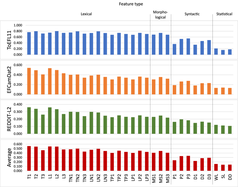
Figure 2: Visual comparison among the accuracy values deriving from the various feature sets for the NLI multi-class classification task. The exact values are reported in Table 6.

Table 6: Accuracy results for the L1 identification task, obtained by using only the features indicated on the row on the dataset indicated in the column. The five best results for every dataset are highlighted in bold, and the five worst results are highlighted in italic. A visual comparison of the values is shown in Figure 2.

		ToEFL11	EFCamDat2	REDDIT-L2	Average
Lexical	T1	0.766	0.541	0.361	0.654
	T2	0.797	0.493	0.340	0.645
	T3	0.721	0.408	0.261	0.565
	L1	0.750	0.535	0.360	0.643
	L2	0.801	0.497	0.335	0.649
	L3	0.741	0.431	0.269	0.586
	TN1	0.754	0.400	0.300	0.577
	TN2	0.793	0.406	0.297	0.600
	TN3	0.716	0.341	0.240	0.529
	LN1	0.738	0.385	0.298	0.562
	LN2	0.793	0.402	0.290	0.598
	LN3	0.735	0.356	0.247	0.546
	TP1	0.676	0.306	0.226	0.491
	TP2	0.741	0.363	0.251	0.552
	TP3	0.703	0.341	0.231	0.522
	LP1	0.676	0.306	0.226	0.491
	LP2	0.741	0.363	0.251	0.552
	LP3	0.703	0.341	0.231	0.522
Morphological	MS1	0.681	0.306	0.230	0.494
	MS2	0.739	0.354	0.248	0.547
	MS3	0.679	0.321	0.220	0.500
Syntactic	P1	0.363	0.189	0.162	0.276
	P2	0.535	0.263	0.197	0.399
	P3	0.551	0.276	0.184	0.414
	D1	0.339	0.182	0.148	0.261
	D2	0.464	0.227	0.165	0.346
	D3	0.495	0.231	0.153	0.363
Statistical	WL	0.211	0.132	0.122	0.172
	SL	0.160	0.139	0.113	0.150
	DD	0.181	0.131	0.107	0.156

Table 7: Accuracy results for the L1 identification task, tackled by using unions of sets of features. The two best results for every dataset are displayed in bold, and the two worst results are displayed in italic.

		ToEFL11	EFCamDat2	REDDIT-L2	Average
Lexical	T1 T2 T3	0.816	0.548	0.397	0.682
	L1 L2 L3	0.817	0.552	0.394	0.685
	TN1 TN2 TN3	0.809	0.447	0.342	0.628
	LN1 LN2 LN3	0.812	0.446	0.338	0.629
	TP1 TP2 TP3	0.759	0.392	0.277	0.576
	LP1 LP2 LP3	0.759	0.392	0.277	0.576
Morphological	MS1 MS2 MS3	0.762	0.388	0.278	0.575
Syntactic	P1 P2 P3	0.583	0.290	0.191	0.437
	D1 D2 D3	0.518	0.242	0.157	0.380
Statistical	WL SL DD	0.256	0.151	0.129	0.204
(All)	(All)	0.813	0.541	0.390	0.677

Table 6 reports the accuracy results we have obtained for the L1 identification task on our three multiclass datasets. Results are displayed per feature set, since we have run classification experiments in which only one of the 30 sets of features we have defined in Section 4.2 has been used, so as to highlight which types of features work best. As can be observed, even though accuracy differs considerably across the three datasets, the trends are rather similar , i.e., if feature set $x$ works better than feature set $y$ in a dataset, the same tends to happen in the two other datasets too. As a general observation, lexical features perform better if compared to other types of features, whilst the features associated to the worst performance are the statistical ones (i.e., WL, SL, DD), whose figures are indeed very similar across the datasets; but let us analyse this in more detail.

In ToEFL11 lexical features perform extremely well, particularly token and lemma bigrams. Masking the NEs does not have a significant effect, and this is obviously due to the fact that, since ToEFL11 was especially created for NLI tasks, NEs had already been removed by its creators. In the EFCamDat2 dataset too, lexical features outperform other types of features, but this time it is unigrams that lead to the highest accuracy. Interestingly, masking NEs leads to poor performance. This might be a consequence of the type of essays the dataset consists of. In fact, EFCamDat2 is made up of writing assignments which, amongst others, prompt the author to write about their life, habits, and so on. Therefore, resorting to NEs might be quite common practice, and, should this be the case, removing them from the texts results in decreased performance. In addition, the importance of NEs is also a possible explanation of the remarkable performance of unigrams (since NEs often consist of one word only).

Accuracy in the REDDIT-L2 dataset is much lower than in ToEFL11 and (to a lesser degree) EFCamDat2, and the differences amongst the various types of features are less substantial than for the two other datasets. The fact that the native language identifier struggles with the REDDIT-L2 posts might be due to two factors: (a) text length, and/or (b) the proficiency level of Reddit.com authors. First, Reddit.com posts tend to be brief, and this might provide the machine with too few significant patterns. The other possible reason has to do, as mentioned above, with the level of proficiency in English of non-native speakers who are active users of the social medium. Whilst the ToEFL11 and the EFCamDat2 datasets rely on the production of learners of English, Reddit.com users are generally fluent in English and interact naturally with their peers. If the overall English level is high, it might be harder to find discriminant features that markedly separate L1 groups, as the L2 production will be quite homogeneous and close to that of native authors.

It is also interesting to compare the performance levels delivered by unigrams, bigrams, and trigrams, respectively. Figure 2 makes it visually apparent that, when it comes to lexical features, unigrams perform better than bigrams and much better than trigrams; this indicates that learners from different L1 groups differ in their choice of words (which is intuitive), rather than in their choice of word groups. The opposite can be observed for syntactic features, where trigrams work better than bigrams and much better than unigrams; this indeed makes sense, since it indicates that different L1 groups differ in their preferred syntactic constructions, rather than in using one part of speech more often than another.

Table 7 displays classification accuracy values averaged across unigrams, bigrams, and trigrams of the same type; we display the results in this way in order to highlight the different contributions of the different types of features, irrespective of the size of the $n$-gram. In this table, the “All” setup refers to an experiment in which all the features are used simultaneously . It is immediately evident from this table that, in all the three datasets, the most discriminative features for the NLI task are the lexical ones, followed by the morphological, syntactic, and statistical features, in this order. The lexical features are so dominant that the two best types (the T and L types) even deliver better performance than all the features taken together; this is somehow unusual for SVMs, which are notoriously so robust to overfitting that, in general, “the more features, the better”. This fact unequivocally shows that word choice is, more than anything, what gives an L1 speaker away.

Table 8: Accuracy results for the L1-vs-EN binary classification task on ToEFL11/LOCNESS. Each cell represents the accuracy obtained when the L1 is the one on the column, using just the features indicated on the row.

		ARA	CHI	FRE	GER	HIN	ITA	JPN	KOR	SPA	TEL	TUR	Average
Lexical	T1	0.992	0.997	0.997	0.998	0.997	0.998	0.999	0.997	0.997	0.999	0.995	0.997
	T2	0.988	0.996	0.992	0.994	0.994	0.993	0.996	0.994	0.991	0.996	0.990	0.993
	T3	0.970	0.988	0.983	0.990	0.983	0.984	0.989	0.984	0.980	0.982	0.977	0.983
	L1	0.991	0.999	0.997	0.999	0.998	0.999	0.998	0.995	0.997	0.998	0.996	0.997
	L2	0.986	0.997	0.994	0.996	0.998	0.997	0.996	0.996	0.991	0.998	0.992	0.995
	L3	0.981	0.992	0.986	0.990	0.987	0.992	0.989	0.990	0.984	0.987	0.985	0.988
	TN1	0.990	0.997	0.997	0.998	0.996	0.998	0.998	0.996	0.997	0.999	0.995	0.996
	TN2	0.988	0.996	0.991	0.995	0.993	0.994	0.996	0.993	0.991	0.996	0.988	0.993
	TN3	0.972	0.989	0.984	0.991	0.983	0.986	0.991	0.984	0.980	0.984	0.976	0.984
	LN1	0.992	0.998	0.997	0.998	0.996	0.999	0.998	0.994	0.997	0.998	0.996	0.997
	LN2	0.989	0.997	0.994	0.995	0.996	0.996	0.997	0.995	0.991	0.997	0.991	0.994
	LN3	0.980	0.991	0.986	0.991	0.987	0.990	0.991	0.990	0.982	0.987	0.982	0.987
	TP1	0.977	0.991	0.984	0.986	0.981	0.985	0.988	0.982	0.980	0.988	0.978	0.984
	TP2	0.979	0.991	0.988	0.991	0.988	0.990	0.992	0.988	0.982	0.991	0.985	0.988
	TP3	0.973	0.988	0.986	0.984	0.980	0.983	0.984	0.982	0.978	0.985	0.975	0.982
	LP1	0.976	0.988	0.980	0.981	0.978	0.981	0.985	0.981	0.978	0.986	0.977	0.982
	LP2	0.977	0.989	0.984	0.988	0.986	0.988	0.990	0.986	0.980	0.990	0.982	0.986
	LP3	0.970	0.984	0.981	0.983	0.978	0.981	0.981	0.980	0.976	0.984	0.976	0.980
Morphological	MS1	0.984	0.991	0.987	0.989	0.986	0.991	0.989	0.986	0.983	0.993	0.984	0.988
	MS2	0.979	0.990	0.990	0.989	0.989	0.991	0.991	0.987	0.984	0.990	0.985	0.988
	MS3	0.965	0.983	0.973	0.980	0.974	0.976	0.986	0.978	0.968	0.979	0.971	0.976
Syntactic	P1	0.925	0.938	0.933	0.932	0.923	0.921	0.929	0.914	0.930	0.924	0.915	0.926
	P2	0.980	0.995	0.991	0.985	0.986	0.984	0.989	0.992	0.990	0.988	0.986	0.988
	P3	0.974	0.995	0.990	0.983	0.987	0.980	0.987	0.987	0.988	0.983	0.985	0.985
	D1	0.826	0.839	0.828	0.847	0.799	0.825	0.865	0.858	0.835	0.815	0.788	0.830
	D2	0.913	0.941	0.918	0.930	0.912	0.921	0.956	0.939	0.915	0.924	0.904	0.925
	D3	0.923	0.957	0.930	0.938	0.924	0.940	0.968	0.953	0.928	0.940	0.925	0.939
Statistical	WL	0.713	0.693	0.656	0.652	0.624	0.650	0.680	0.662	0.675	0.623	0.594	0.657
	SL	0.554	0.715	0.722	0.765	0.733	0.631	0.720	0.723	0.680	0.704	0.713	0.696
	DD	0.391	0.521	0.399	0.459	0.344	0.440	0.574	0.562	0.401	0.383	0.547	0.456

Table 9: As Table 8, but with EFCamDat2/LOCNESS in place of ToEFL11/LOCNESS.

		ARA	CHI	FRE	GER	HIN	ITA	JPN	KOR	RUS	SPA	TUR	Average
Lexical	T1	0.990	0.992	0.993	0.990	0.992	0.993	0.991	0.990	0.994	0.989	0.993	0.992
	T2	0.981	0.985	0.985	0.985	0.990	0.985	0.985	0.986	0.986	0.982	0.987	0.985
	T3	0.955	0.971	0.973	0.971	0.971	0.971	0.971	0.970	0.977	0.961	0.968	0.969
	L1	0.989	0.992	0.995	0.992	0.991	0.993	0.991	0.987	0.992	0.989	0.993	0.991
	L2	0.984	0.987	0.986	0.990	0.991	0.988	0.987	0.985	0.988	0.982	0.987	0.987
	L3	0.967	0.974	0.975	0.974	0.978	0.974	0.978	0.974	0.978	0.966	0.975	0.974
	TN1	0.987	0.990	0.990	0.990	0.992	0.990	0.988	0.988	0.992	0.988	0.991	0.990
	TN2	0.980	0.982	0.984	0.984	0.987	0.984	0.983	0.984	0.986	0.981	0.986	0.984
	TN3	0.958	0.974	0.974	0.972	0.972	0.970	0.969	0.971	0.977	0.960	0.970	0.970
	LN1	0.986	0.990	0.991	0.991	0.992	0.990	0.988	0.985	0.992	0.986	0.991	0.989
	LN2	0.983	0.986	0.985	0.989	0.988	0.986	0.985	0.983	0.987	0.981	0.986	0.985
	LN3	0.965	0.977	0.975	0.974	0.977	0.973	0.973	0.973	0.977	0.966	0.974	0.973
	TP1	0.973	0.979	0.979	0.971	0.980	0.980	0.975	0.975	0.981	0.966	0.981	0.976
	TP2	0.974	0.984	0.979	0.977	0.985	0.983	0.977	0.981	0.985	0.973	0.983	0.980
	TP3	0.961	0.978	0.972	0.968	0.977	0.973	0.972	0.974	0.977	0.960	0.977	0.972
	LP1	0.947	0.958	0.961	0.961	0.968	0.970	0.966	0.975	0.972	0.956	0.971	0.968
	LP2	0.948	0.954	0.962	0.967	0.965	0.963	0.966	0.971	0.972	0.963	0.972	0.972
	LP3	0.931	0.943	0.952	0.958	0.956	0.953	0.957	0.965	0.967	0.951	0.966	0.967
Morphological	MS1	0.975	0.980	0.981	0.974	0.986	0.984	0.976	0.980	0.981	0.970	0.985	0.979
	MS2	0.974	0.982	0.980	0.982	0.987	0.980	0.979	0.982	0.983	0.973	0.985	0.981
	MS3	0.954	0.969	0.966	0.963	0.970	0.962	0.967	0.971	0.974	0.959	0.972	0.966
Syntactic	P1	0.947	0.965	0.946	0.944	0.962	0.951	0.957	0.958	0.959	0.932	0.968	0.954
	P2	0.961	0.975	0.970	0.968	0.975	0.971	0.967	0.970	0.973	0.955	0.975	0.969
	P3	0.960	0.981	0.968	0.966	0.979	0.973	0.972	0.977	0.974	0.956	0.977	0.971
	D1	0.926	0.941	0.921	0.923	0.935	0.911	0.931	0.936	0.938	0.901	0.948	0.928
	D2	0.943	0.960	0.950	0.945	0.955	0.941	0.949	0.955	0.955	0.928	0.967	0.950
	D3	0.946	0.967	0.954	0.947	0.962	0.946	0.953	0.963	0.960	0.937	0.972	0.955
Statistical	WL	0.863	0.893	0.867	0.847	0.892	0.873	0.880	0.885	0.885	0.843	0.887	0.874
	SL	0.861	0.888	0.876	0.878	0.888	0.854	0.900	0.910	0.905	0.839	0.922	0.884
	DD	0.836	0.873	0.862	0.863	0.886	0.828	0.895	0.903	0.891	0.820	0.912	0.870

Table 10: As Table 8, but with REDDIT-L2/REDDIT-UK in place of ToEFL11/LOCNESS.

		FIN	FRE	GER	ITA	NED	NOR	POL	POR	ROM	SPA	SWE	Average
Lexical	T1	0.764	0.784	0.786	0.758	0.739	0.749	0.774	0.774	0.771	0.757	0.758	0.765
	T2	0.752	0.772	0.778	0.740	0.725	0.738	0.770	0.762	0.762	0.744	0.735	0.753
	T3	0.701	0.710	0.725	0.688	0.671	0.685	0.716	0.701	0.704	0.681	0.674	0.696
	L1	0.760	0.781	0.780	0.757	0.737	0.745	0.774	0.771	0.767	0.758	0.753	0.762
	L2	0.758	0.774	0.780	0.739	0.726	0.741	0.768	0.760	0.765	0.744	0.739	0.754
	L3	0.707	0.726	0.731	0.689	0.684	0.695	0.725	0.710	0.711	0.695	0.682	0.705
	TN1	0.739	0.763	0.764	0.735	0.715	0.729	0.752	0.752	0.752	0.735	0.737	0.743
	TN2	0.739	0.756	0.762	0.725	0.710	0.724	0.760	0.752	0.751	0.731	0.724	0.739
	TN3	0.693	0.704	0.717	0.681	0.656	0.676	0.711	0.697	0.697	0.675	0.665	0.688
	LN1	0.733	0.762	0.757	0.732	0.713	0.726	0.756	0.753	0.751	0.738	0.730	0.741
	LN2	0.740	0.762	0.766	0.726	0.711	0.725	0.758	0.752	0.755	0.736	0.726	0.742
	LN3	0.700	0.720	0.721	0.684	0.668	0.688	0.722	0.708	0.706	0.687	0.675	0.698
	TP1	0.702	0.728	0.725	0.695	0.675	0.695	0.729	0.719	0.718	0.700	0.691	0.707
	TP2	0.711	0.742	0.739	0.700	0.687	0.709	0.743	0.733	0.729	0.707	0.696	0.718
	TP3	0.688	0.704	0.707	0.671	0.654	0.676	0.719	0.697	0.698	0.673	0.661	0.686
	LP1	0.692	0.701	0.703	0.659	0.644	0.675	0.703	0.701	0.689	0.680	0.671	0.689
	LP2	0.702	0.714	0.711	0.681	0.657	0.689	0.714	0.713	0.702	0.687	0.676	0.701
	LP3	0.655	0.674	0.677	0.632	0.634	0.645	0.691	0.669	0.669	0.657	0.643	0.668
Morphological	MS1	0.706	0.733	0.727	0.701	0.681	0.695	0.724	0.724	0.720	0.699	0.692	0.709
	MS2	0.705	0.732	0.739	0.699	0.681	0.704	0.735	0.726	0.723	0.698	0.691	0.712
	MS3	0.674	0.691	0.699	0.663	0.644	0.666	0.706	0.683	0.685	0.661	0.651	0.675
Syntactic	P1	0.601	0.640	0.627	0.611	0.593	0.605	0.659	0.629	0.623	0.608	0.599	0.618
	P2	0.638	0.677	0.663	0.642	0.622	0.643	0.688	0.678	0.665	0.645	0.627	0.653
	P3	0.631	0.665	0.648	0.632	0.604	0.631	0.681	0.656	0.657	0.633	0.613	0.641
	D1	0.608	0.617	0.609	0.597	0.586	0.598	0.657	0.607	0.617	0.607	0.588	0.608
	D2	0.610	0.638	0.624	0.616	0.585	0.606	0.666	0.630	0.632	0.605	0.589	0.618
	D3	0.603	0.629	0.618	0.602	0.578	0.608	0.646	0.616	0.621	0.605	0.585	0.610
Statistical	WL	0.576	0.587	0.557	0.564	0.563	0.571	0.588	0.588	0.588	0.550	0.571	0.573
	SL	0.540	0.501	0.529	0.500	0.570	0.511	0.548	0.506	0.549	0.497	0.568	0.529
	DD	0.560	0.548	0.523	0.535	0.566	0.552	0.580	0.550	0.554	0.543	0.566	0.552

5.2 Results of the binary experiments: Predicting if the speaker is native or non-native

Tables 8, 9, 10 show how each feature set performs in the L1-vs-EN binary tasks on the different datasets used. Compared to the multiclass NLI task, accuracy is much higher for every feature set on every dataset. This time, most feature sets behave well, especially ToEFL11/LOCNESS and EFCamDat2/LOCNESS, except for statistical features, which perform worse than the others on all the datasets.

Accuracy on the ToEFL11/LOCNESS and EFCamDat2/LOCNESS corpora is very high in many cases, especially for lexical features, which often give rise to accuracy values in the 0.96–0.99 range. In EFCamDat2/LOCNESS even the statistical features (WL, SL, DD) give rise to high accuracy values. We conjecture this to be caused by the differences in context and motivations that underlie the LOCNESS documents with respect to the ToEFL11 and EFCamDat2 documents, which makes the task of separating LOCNESS from the other two easier.

Conversely, REDDIT-L2/REDDIT-UK uses the same source for non-native and native documents, thus factoring out the aspects that make L1-vs-EN classification easier for the other two datasets. Accuracy values are thus lower than in ToEFL11/LOCNESS and EFCamDat2/LOCNESS, while still very good. Here, the statistical features have accuracy scores that are close to those of the random classifier (whose expected accuracy is 0.5), indicating that there are hardly any significant differences in the phenomena they represent (i.e., word length, sentence length, and dependency depth) between native production and non-native production, and that any clue used by the learning algorithm to make a correct prediction is based on lexical / morphological / syntactic features.

It is relevant to note that, for all corpora, no L1 emerges as significantly harder or easier to recognise with respect to the others, and that no L1 shows a different trend in the relative accuracy scored by the different types of features.

5.3 Feature analysis: Lexical, morphological, and syntactic features

In order to show the power of SVM-based explainable machine learning for characterising language transfer, we analyse the results of multiclass classification for NLI, and we draw our examples from two sample L1s, Spanish and Italian, as emerging from two sample datasets, EFCamDat2 and ToEFL11. (We concentrate on EFCamDat2 and ToEFL11 because they are the two datasets on which the best accuracy is reached, so the intuitions about feature importance that we can draw from them are more reliable.) Similar analyses can be carried out on other L1s, on other datasets, and on the L1-vs-EN task.

In order to gain insight into L1-specific patterns, we look at the features that the machine deemed most discriminant for each language group. In order to do this, we inspect the parameter values (hereafter: “coefficients”) that the SVM assigned to each feature in the “All” experiment reported in Table 7; as explained in Section 3, a coefficient determines how the value of the corresponding feature’s relative frequency in a document contributes to the classification decision for that document, with coefficients of high absolute magnitude indicating a large impact on the decision, and with the sign of the coefficient indicating whether this value weighs towards assigning ($+$) or not assigning ($-$) the corresponding L1. In other words, positive coefficients identify overuse patterns, whilst negative coefficients identify underuse patterns.

It must be pointed out that overuse and underuse patterns emerge from a contrastive L2-based perspective, i.e., by comparing the written output of one linguistic group to that of all the other linguistic groups. As a consequence, the linguistic behaviour of an L1 group must be viewed as a relative rather than an absolute phenomenon. What can be observed are indeed discriminant linguistic deviations that characterise specific L1 groups only with reference to the other L1 groups. Such deviations can occasionally coincide, but not necessarily, with errors (e.g., spelling mistakes typical of one particular L1 group).

5.3.1 Case Study 1: Spanish as L1 in EFCamDat2.

In EFCamDat2, the coefficients with the highest absolute magnitude turn out to correspond to named entities. In view of what we said in Section 4.2.1, this is unsurprising, since many essays of which EFCamDat2 consists of deal, as discussed in Section 4.1.1, with everyday experiences of the speakers; as such, they are likely to contain many named entities that refer to the local culture / environment of the speaker, and that thus “give away” the nationality of the speaker. However, named entities are uninteresting to our goals, and we thus do not discuss them; we thus discuss features other than named entities, starting with lexical features that play an important role for specific L1s.

In the case of Spanish learners, the machine identified two particularly discriminant features in EFCamDat2, i.e., the use of the words *de (coefficient: $+$2.74) and *diferent (coefficient: $+$2.49). By examining some usage examples (e.g., de train or de evening), we noticed that the former is a misspelling of the determiner the, likely influenced by the phonology of Spanish. Indeed, since Spanish does not exhibit the phoneme /ð/, Spanish learners of English approximate the voiced interdental fricative to the dental sound /d/, which, conversely, belongs in the Spanish phonological system. Interestingly, voice prevails over manner and place of articulation. In fact, Spanish does make use of the phoneme //, which is the unvoiced counterpart of /ð/. Yet, learners instinctively approximate the latter to /d/.

As to the misspelling of the adjective different, it appears to follow the spelling of the Spanish equivalent diferente, in which the double consonant ff is reduced to a single consonant, following its pronunciation. It must be noted that, amongst the observed examples involving the term different, instances of pluralisation of the adjective can be detected (e.g., *diferents areas or *diferents types), brought about by the agreement rules of Spanish.

Although Spanish learners exhibit a distinct tendency to start a new sentence with the adverb never (coefficient: $+$2.42) more often than learners from other L1 backgrounds, e.g., never forget your family (…) or never the ball must touch (…), this fact cannot be directly linked to language transfer. On the contrary, overuse of the bigram because is (coefficient: $+$1.97) as in the examples because is ugly or because is very strange point to the omission of the dummy pronoun, typical of the Spanish language.

In terms of underuse patterns, the most relevant habits captured by the machine concern the beginning of new sentences. The machine assigned the highest coefficients to the bigrams “. so” (coefficient: $-$2.34), “. but” (coefficient: $-$1.74), and “. and” (coefficient: $-$1.52), a sign that Spanish learners tend to avoid starting a new sentence with so, but and and, just as they would do in their mother tongue.

5.3.2 Case Study 2: Italian as L1 in ToEFL11.

Differently from the case study discussed in Section 5.3.1, here the coefficients with the highest absolute magnitude do not belong to named entities, for the simple reason that, as mentioned in Section 5.1, named entities were masked off from ToEFL11 directly by its creators.

The most relevant feature marking the production of Italian learners in the ToEFL11 dataset is the trigram I think that preceded by punctuation or by another word. The pattern appears with a coefficient of $+$3.84. Its presence can be accounted for by the nature of the TOEFL exam, in which students are often prompted to give their opinion on a variety of topics. However, if its appearance were the sole result of following the writing instructions, it should be evenly distributed across the different L1s, and therefore lose its importance as a feature. Rather, its high incidence in the writings of Italian learners vouches for its significance. Consistent resort to the above-mentioned expression could indeed stem from the convenient and safe equivalence between the Italian penso che and the English I think that. A further hypothesis could be that Italian speakers simply employ (in their mother tongue) the phrase penso che with greater frequency compared to other L1 speakers. Yet, evidence from comparable corpora should be provided to support this thesis.

The second most discriminant feature in the ToEFL11 dataset is the bigram “token + :” to which the machine assigned a coefficient of +3.71. The use of the colon in English is indeed problematic for Italian learners. In fact, in Italian, the colon can be either used to introduce a list of items or to illustrate a concept, whilst in English only the former is allowed. By looking into the occurrences of “token + :”, we were able to identify many examples of misuse (e.g., one thing seems clear: long term scars or you take a risk: you change your type of), which can account for the high number of occurrences of the pattern.

Typical of Italian learners is the trigram “. in fact” (coefficient: $+$2.98) together with its misspelt alternative form *infact (coefficient: $+$2.94). The latter can also be found in the EFCamDat2 dataset with a coefficient of $+$2.87. In Italian, infatti is a highly occurring word. Nevertheless, despite a superficial resemblance, in fact and infatti have different meanings and functions. The former provides more detailed information about a topic previously introduced. The latter confirms something that was previously stated by means of a causal relationship. Examples of misuse in ToEFL11 are he or she takes risks. In fact, in the business world if (…) or I think in fact that a specialised worker has (…).

Particularly distinctive in ToEFL11 (coefficient: $+$2.69) are reporting verbs (believe, decide, and think) followed by a that-clause and governing a subject.

From a strictly lexical point of view, two lemmas are very relevant in ToEFL11 as they mark the production of Italian learners: the adverb probably (coefficient: $+$2.59) and the noun possibility (coefficient: $+$2.45). The former is occasionally misplaced in a way that can be traced back to Italian syntax, e.g., a question that probably I will present to myself.

As regards patterns of underuse, the most discriminating feature is the verb get which exhibits a coefficient of $-$3.07. Indeed, compared to other L1 speakers of English, Italians are reluctant to use such a verb. Moreover, they seem to rarely start a new sentence with a conjunction, a fact that can be accounted for by the stylistic rules of written Italian, which do not allow for such a pattern.

5.4 Feature analysis: Statistical features

Although statistical features (WL, SL, DD) do not seem to be very helpful in discriminating the different L1s, they can nonetheless be investigated in order to gather information concerning the linguistic habits of speakers of English from different linguistic backgrounds. In this section we compare the values taken by the statistical features with respect to two orthogonal dimensions, i.e., the L1 and the proficiency level.

Table 11: Average values of the statistical features for each language group on the EFCamDat2 dataset.

	avg WL	avg SL	avg DD
ARA	3.76	11.64	2.16
CHI	3.76	11.86	2.10
FRE	3.82	12.59	2.21
GER	3.94	13.18	2.29
HIN	3.77	11.68	2.09
ITA	3.89	14.11	2.41
JPN	3.80	11.18	2.03
KOR	3.70	10.61	1.95
SPA	3.84	13.12	2.26
RUS	3.87	11.91	2.19
TUR	3.75	10.37	1.94
(All)	3.83	12.13	2.17

Table 11 shows information on the average values of the statistical features for each language group on the EFCamDat2 dataset. German learners have a slightly higher word length average than other L1s, with Italians in second place. Italian, German, Spanish, and French learners produce longer sentences if compared to other L1s. Conversely, Turkish and Korean learners tend to be more succinct, with the shorter sentence length (almost four words of difference between Italian and Korean) also reflected by a smaller depth in the parse tree.

EFCamDat2 essays are rated by 16 proficiency levels, 1 being the lowest and 16 being the highest. We grouped essays by three ranges of proficiency levels, thus deriving three subsets of the original EFCamDat2: low (EFCamDat2-G1), containing essay in levels 1 to 5 included; intermediate (EFCamDat2-G2), for levels 6 to 12; and advanced (EFCamDat2-G3), for levels 13 and higher. We compare the frequency distribution of the statistical features across these three proficiency groups.

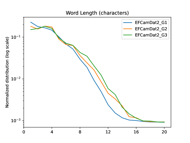
Figure 3: Comparison of normalized distribution of word length across proficiency groups in EFCamDat2.

If we look at word length (Figure 3) we can observe that it increases at the increase of the proficiency level (a shift towards right, i.e., towards longer words, of the curve of the distribution). (Average word length for documents in EFCamDat2-G1 is 3.49, for EFCamDat2-G2 is 3.85, and for EFCamDat2-G3 is 4.12.) This is unsurprising because longer words are, on average, less common in language use, and the use of longer words denotes higher sophistication in a learner’s active vocabulary.

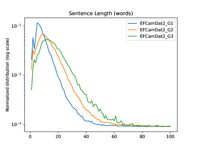
Figure 4: Comparison of normalized distribution of sentence length across proficiency groups in EFCamDat2.

Sentence length (Figure 4) follows a similar pattern, with longer sentences being produced, on average, by more proficient learners. Learners with a smaller command of their L2 tend to produce shorter sentences, composed on average of 8.9 words; this number doubles for the top proficiency group EFCamDat2-G3, with an average length of 16.7 words, while group EFCamDat2-G2 places almost exactly in the middle, with an average sentence length of 12.8 words.

The length of the sentence is obviously correlated with its complexity, and thus with the depth of the dependency tree. This is confirmed by the comparison of the frequency distributions of feature DD (Figure 5): the lower proficiency group contains sentences with a more shallow structure (average depth: 1.75), and depth increases as proficiency improves (average depth: 2.18 for EFCamDat2-G2 and 2.57 for EFCamDat2-G3). All in all, this is also unsurprising, since more proficient learners have a higher command of the syntax of the L2, and thus venture more often into more complex syntactic structures and, as a consequence, into longer sentences.

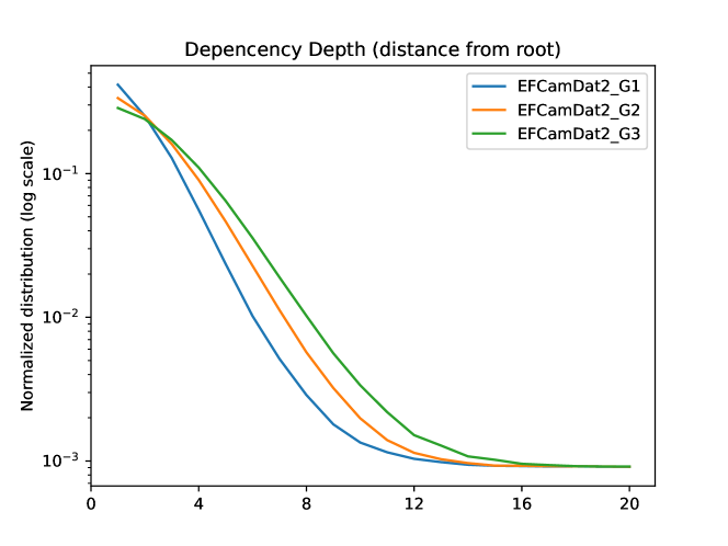
Figure 5: Comparison of normalized distribution of dependency depth (i.e., distance from root of the dependency tree) across proficiency groups in EFCamDat2.

6 Conclusion

Explainable machine learning (EML) can be a very powerful tool to investigate second language acquisition, and language transfer in particular, especially when sizeable amounts of learner data for a variety of different languages are available. We have shown how interesting facts about language transfer emerge from the analysis of the parameters of classifiers trained to perform native language identification or native vs. non-native classification. The classifiers we have discussed in this paper were trained via support vector machines, but also other classifier-learning methods, such as logistic regression, produce similarly interpretable classifiers. Each parameter of the SVM classifier is associated to a feature, i.e., a linguistic trait whose frequency of occurrence in the different classes of interest (i.e., native speakers, non-native speakers, non-native speakers of a specific L1) we want to exploit in order to perform classification. Features to which the learning algorithm has associated a value of high absolute magnitude represent linguistic traits whose usage patterns significantly differ across the classes of interest, with a positive value weighing towards assigning the class and a negative value weighing against assigning it. We have shown, by drawing examples from two among the classes we have investigated (Spanish learners of English and Italian learners of English) how the parameters that are assigned the values with the highest magnitude are indeed associated with linguistic traits that are well-known to characterize the linguistic production of those speakers. This shows that performing native language identification, or native vs. non-native classification, via an EML algorithm, can be a valuable tool for the scholar who investigates second language acquisition and language transfer.

Where could improvements to these results come from? One promising line of research could involve new EML methods. While until a few years ago it was generally accepted that ML algorithms could generate “black box” (i.e., hardly inspectable) classifiers, the push towards EML has increased in the last ten years, due to the fact that ML algorithms are more and more frequently applied to high-stakes domains (e.g., algorithms that decide if a convict should be granted parole, algorithms that decide if a loan application should be considered favourably or not, etc.), and that their decisions cannot be accepted without an accompanying justification. Unfortunately, most research on EML so far has targeted structured (i.e., tabular) data, and many proposed solutions are hardly applicable to textual data because of the high dimensionality of the latter. More research on EML for text is needed, and this would hold promise for our application context.

Another factor of key importance for research on language transfer is the quality of the available datasets. First, datasets of higher quality than the ones we have used here could deliver more accurate classifiers, which would allow drawing more reliable intuitions about language transfer. An important step towards higher-quality datasets would derive from having data in which the mother tongue of the speaker is explicit; in the datasets we have used we can only estimate the speaker’s L1 from its nationality / country of residence, but these latter attributes are not always in a 1-to-1 correspondence with mother tongue, so it is not clear how many of the inaccurate decisions that today’s classifier return are due to mislabelled training documents or mislabelled test documents. Another important improvement might come from having better quality native vs. non-native datasets than ToEFL11/LOCNESS and EFCamDat2/LOCNESS. These latter derive from the union of two datasets (a native dataset and a non-native dataset) consisting of two different types of text, which makes the binary classification task easier than it should be; the availability of more homogeneous native vs. non-native datasets (such as REDDIT-L2/REDDIT-UK) would thus be an important step towards addressing the (still under-researched problem) of native vs. non-native classification.

References

- Aarts and Granger, (1998) Aarts, J. and Granger, S. (1998). Tag sequences in learner corpora: A key to interlanguage grammar and discourse. In Granger, S., editor, Learner English on Computer, pages 141–150. Longman, London, UK.
- Aijmer and Altenberg, (2013) Aijmer, K. and Altenberg, B., editors (2013). Advances in corpus-based contrastive linguistics: Studies in honour of Stig Johansson. John Benjamins Publishing, Amsterdam, NL.
- Altenberg and Tapper, (1998) Altenberg, B. and Tapper, M. (1998). The use of adverbial connectors in advanced Swedish learners’ written English. In Granger, S., editor, Learner English on Computer, pages 80–93. Longman, London, UK.
- Anand Kumar et al., (2018) Anand Kumar, M., Barathi Ganesh, H., Ajay, S., and Soman, K. P. (2018). Overview of the second shared task on Indian native language identification (INLI). In Working Notes of the Forum for Information Retrieval Evaluation (FIRE 2018), pages 39–50, Gandhinagar, IN.
- Anand Kumar et al., (2017) Anand Kumar, M., Barathi Ganesh, H., Singh, S., Soman, K. P., and Rosso, P. (2017). Overview of the INLI PAN at FIRE 2017 track on indian native language identification. In Working notes of the Forum for Information Retrieval Evaluation (FIRE 2017), pages 99–105, Bangalore, IN.
- Bardovi-Harlig and Sprouse, (2018) Bardovi-Harlig, K. and Sprouse, R. A. (2018). Negative versus positive transfer. In Liontas, J. I., editor, The TESOL Encyclopedia of English Language Teaching, pages 1–6. Wiley Academic Publishers, New York, US.
- Basile and Lana, (2008) Basile, C. and Lana, M. (2008). L’attribuzione di testi con metodi quantitativi: Riconoscimento di testi gramsciani. In Atti del Convegno Nazionale dell’Associazione Italiana Terminologia, pages 177–195, Cosenza, IT.
- Beare, (2000) Beare, S. (2000). Differences in content generating and planning processes of adult L1 and L2 proficient writers. PhD thesis, University of Ottawa, Ottawa, CA.
- Belle and Papantonis, (2021) Belle, V. and Papantonis, I. (2021). Principles and practice of explainable machine learning. Frontiers in Big Data, 4:688969.
- Binongo, (2003) Binongo, J. N. (2003). Who wrote the 15th Book of Oz? An application of multivariate analysis to authorship attribution. Chance, 16(2):9–17.
- Blanchard et al., (2013) Blanchard, D., Tetreault, J., Higgins, D., Cahill, A., and Chodorow, M. (2013). TOEFL11: A corpus of non-native English. Technical Report RR–13-24, Educational Testing Service, Princeton, US.
- Brooke and Hirst, (2011) Brooke, J. and Hirst, G. (2011). Native language detection with ‘cheap’ learner corpora. In Proceedings of the 2011 Conference on Learner Corpus Research, Louvain-la-Neuve, BE.
- Carrió Pastor, (2012) Carrió Pastor, M. (2012). A contrastive analysis of epistemic modality in scientific English. Revista de Lengua para Fines Específicos, 18:115–132.
- Corbara et al., (2019) Corbara, S., Moreo, A., Sebastiani, F., and Tavoni, M. (2019). The Epistle to Cangrande through the lens of computational authorship verification. In Proceedings of the 1st International Workshop on Pattern Recognition for Cultural Heritage (PatReCH 2019), pages 148–158, Trento, IT.
- Corder, (1967) Corder, S. P. (1967). The significance of learner’s errors. International Review of Applied Linguistics in Language Teaching, 5(1-4):161–170.
- Dušková, (1969) Dušková, L. (1969). On sources of errors in foreign language learning. International Review of Applied Linguistics in Language Teaching, 7(1):11–36.
- Fries, (1945) Fries, C. C. (1945). Teaching and learning English as a foreign language. University of Michigan Press, Ann Arbor, US.
- Geertzen et al., (2013) Geertzen, J., Alexopoulou, D., and Korhonen, A. M. (2013). Automatic linguistic annotation of large-scale L2 databases: The EF-Cambridge Open Language Database (EFCAMDAT). In Proceedings of the 31st Second Language Research Forum (SLRF 2012), pages 1–15, Pittsburgh, US.
- Ginzburg, (1989) Ginzburg, C. (1989). Clues: Roots of an evidential paradigm. In Clues, Myths, and the Historical Method: Works of Carlo Ginzburg, pages 96–214. The Johns Hopkins University Press, Baltimore, US.
- Goldin et al., (2018) Goldin, G., Rabinovich, E., and Wintner, S. (2018). Native language identification with user generated content. In Proceedings of the 2018 Conference on Empirical Methods in Natural Language Processing (EMNLP 2018), pages 3591–3601, Brussels, BE.
- Granger, (1998) Granger, S. (1998). The computer learner corpus: A versatile new source of data for SLA research. In Granger, S., editor, Learner English on Computer, pages 3–18. Longman, London, UK.
- Granger et al., (2009) Granger, S., Dagneaux, E., Meunier, F., and Paquot, M. (2009). International Corpus of Learner English. Presses Universitaires de Louvain, Louvain-la-Neuve, BE, 2nd edition.
- Gullberg, (2011) Gullberg, M. (2011). Thinking, speaking and gesturing about motion in more than one language. In Pavlenko, A., editor, Thinking and Speaking in Two Languages, pages 143–169. Multilingual Matters, Bristol, UK.
- Huang et al., (2018) Huang, Y., Murakami, A., Alexopoulou, T., and Korhonen, A. (2018). Dependency parsing of learner english. International Journal of Corpus Linguistics, 23(1):28–57.
- Italia and Canettieri, (2013) Italia, P. and Canettieri, P. (2013). Un caso di attribuzionismo novecentesco: Il “Diario Postumo” di Montale. Cognitive Philology, 6.
- Jarvis and Crossley, (2012) Jarvis, S. and Crossley, S. A., editors (2012). Approaching language transfer through text classification explorations in the detection-based approach. Multilingual Matters, Bristol, UK.
- Jiang et al., (2014) Jiang, X., Guo, Y., Geertzen, J., Alexopoulou, D., Sun, L., and Korhonen, A. (2014). Native language identification using large longitudinal data. In Proceedings of the 9th International Conference on Language Resources and Evaluation (LREC 2014), pages 3309–3312, Reykjavik, IS.
- Jordan and Mitchell, (2015) Jordan, M. I. and Mitchell, T. M. (2015). Machine learning: Trends, perspectives, and prospects. Science, 349(6245):255–260.
- Kabala, (2020) Kabala, J. (2020). Computational authorship attribution in medieval Latin corpora: The case of the Monk of Lido (ca. 1101–08) and Gallus Anonymous (ca. 1113–17). Language Resources and Evaluation, 54(1):25–56.
- Kestemont et al., (2015) Kestemont, M., Moens, S., and Deploige, J. (2015). Collaborative authorship in the twelfth century: A stylometric study of Hildegard of Bingen and Guibert of Gembloux. Digital Scholarship in the Humanities, 30(2):199–224.
- Koppel and Winter, (2014) Koppel, M. and Winter, Y. (2014). Determining if two documents are written by the same author. Journal of the Association for Information Science and Technology, 65(1):178–187.
- Krashen, (1983) Krashen, S. (1983). Newmark’s “ignorance hypothesis” and current second language acquisition theory. In Gass, S. M. and Selinker, L., editors, Language transfer in language learning: Issues in second language research, pages 135–153. Newbury House Publishers, Rowley, US.
- Köhlmyr, (2001) Köhlmyr, P. (2001). To err is human…. : An investigation of grammatical errors in Swedish 16-year-old learners’ written production in English. PhD thesis, University of Gothenburg, Gothenburg, SE.
- Lado, (1957) Lado, R. (1957). Linguistics across cultures. University of Michigan Press, Ann Arbor, US.
- Lutosławski, (1898) Lutosławski, W. (1898). Principes de stylométrie. Revue des Études Grecques, 11(61–81).
- Malmasi, (2016) Malmasi, S. (2016). Native language identification: Explorations and applications. PhD thesis, Macquarie University, Sydney, AU.
- Malmasi and Dras, (2015) Malmasi, S. and Dras, M. (2015). Large-scale native language identification with cross-corpus evaluation. In Proceedings of the 2015 Conference of the North American Chapter of the Association for Computational Linguistics (NAACL 2015), pages 1403–1409, Denver, US.
- Malmasi et al., (2017) Malmasi, S., Evanini, K., Cahill, A., Tetreault, J. R., Pugh, R. A., Hamill, C., Napolitano, D., and Qian, Y. (2017). A report on the 2017 native language identification shared task. In Proceedings of the 12th Workshop on Innovative Use of NLP for Building Educational Applications (BEA@EMNLP 2017), pages 62–75, Copenhagen, DK.
- Meisel et al., (1981) Meisel, J. M., Clahsen, H., and Pienemann, M. (1981). On determining developmental stages in natural second language acquisition. Studies in Second Language Acquisition, 3(2):109–135.
- Mendenhall, (1887) Mendenhall, T. C. (1887). The characteristic curves of composition. Science, 9:237–249.
- Miliander, (2003) Miliander, J. (2003). We get the answer we deserve: A study of vocabulary in a corpus of spoken and written learner English. PhD thesis, Karlstad University Studies, Karlstad, SE.
- Mosteller and Wallace, (1964) Mosteller, F. and Wallace, D. L. (1964). Inference and disputed authorship: The Federalist. Addison-Wesley, Reading, MA.
- Mu and Carrington, (2007) Mu, C. and Carrington, S. (2007). An investigation of three Chinese students’ English writing strategies. TESL-EJ: The Electronic Journal for English as a Second Language, 11(1):1–23.
- Odlin, (1989) Odlin, T. (1989). Language transfer: Cross-linguistic influence in language learning. Cambridge University Press, Cambridge, UK.
- Odlin, (2003) Odlin, T. (2003). Cross-linguistic influence. In Doughty, C. and Long, M., editors, The Handbook of Second Language Acquisition, pages 436–486. Blackwell, London, UK.
- Platt, (2000) Platt, J. C. (2000). Probabilistic outputs for support vector machines and comparison to regularized likelihood methods. In Smola, A., Bartlett, P., Schölkopf, B., and Schuurmans, D., editors, Advances in Large Margin Classifiers, pages 61–74. The MIT Press, Cambridge, MA.
- Rabinovich et al., (2018) Rabinovich, E., Tsvetkov, Y., and Wintner, S. (2018). Native language cognate effects on second-language lexical choice. Transactions of the Association for Computational Linguistics, 6:329–342.
- Rosén, (2006) Rosén, C. (2006). Warum klingt das nicht deutsch?: Probleme der informationsstrukturierung in deutschen texten schwedischer schüler und studenten. PhD thesis, Lund University, Lund, SE.
- Schachter, (1983) Schachter, J. (1983). A new account of language transfer. In Gass, S. M. and Selinker, L., editors, Language transfer in language learning: Issues in second language research, pages 98–111. Newbury House Publishers, Rowley, US.
- Sebastiani, (2002) Sebastiani, F. (2002). Machine learning in automated text categorization. ACM Computing Surveys, 34(1):1–47.
- Selinker, (1972) Selinker, L. (1972). Interlanguage. International Review of Applied Linguistics in Language Teaching, 10(1-4):209–231.
- Stamatatos, (2009) Stamatatos, E. (2009). A survey of modern authorship attribution methods. Journal of the American Society for Information Science and Technology, 60(3):538–556.
- Stamatatos, (2016) Stamatatos, E. (2016). Authorship verification: A review of recent advances. Research in Computing Science, 123:9–25.
- Swan and Smith, (2001) Swan, M. and Smith, B. (2001). Learner English: A teacher’s guide to interference and other problems. Cambridge University Press, Cambridge, UK.
- Tetreault et al., (2013) Tetreault, J., Blanchard, D., and Cahill, A. (2013). A report on the first native language identification shared task. In Proceedings of the 8th Workshop on Innovative Use of NLP for Building Educational Applications (BEA 2013), pages 48–57, Atlanta, US.
- Tetreault et al., (2012) Tetreault, J. R., Blanchard, D., Cahill, A., and Chodorow, M. (2012). Native tongues, lost and found: Resources and empirical evaluations in native language identification. In Proceedings of the 24th International Conference on Computational Linguistics (COLING 2012), pages 2585–2602, Mumbai, IN.
- Tuccinardi, (2017) Tuccinardi, E. (2017). An application of a profile-based method for authorship verification: Investigating the authenticity of Pliny the Younger’s letter to Trajan concerning the Christians. Digital Scholarship in the Humanities, 32(2):435–447.
- Wardhaugh, (1970) Wardhaugh, R. (1970). The contrastive analysis hypothesis. TESOL Quarterly, 4(2):123–130.
- Xia, (2015) Xia, L. (2015). An error analysis of the word class: A case study of Chinese college students. International Journal of Emerging Technologies in Learning, 10(3):41–45.
- Ye, (2004) Ye, Z. (2004). Chinese categorization of interpersonal relationships and the cultural logic of Chinese social interaction: An indigenous perspective. Intercultural Pragmatics, 1:211–230.
- Zhang, (2010) Zhang, Q. (2010). A study of Chinese learning of English tag questions. Journal of Language Teaching and Research, 1(5):578–582.
- Zhang, (2011) Zhang, X. (2011). Support vector machines. In Sammut, C. and Webb, G. I., editors, Encyclopedia of Machine Learning, pages 941–946. Springer, Heidelberg, DE.