Risk in Network Economies

Abstract

Economic models with input-output networks assume that firm or sector (unit) growth is driven by a weighted sum of trade partners’ growth and an independently-drawn idiosyncratic shock. I show that the idiosyncratic risk assumption in a broad class of network models implicitly generates restrictions on the network weights which are unrealistic. When allowing for correlated shocks, units are exposed to an additional risk term which captures the ability to substitute away from supply and demand shocks propagating through the network. I provide empirical evidence that changes in substitutability between trade partners are inversely related to changes in the panel of realized industry variance. Moreover, I find that supply-side (demand-side) substitutability is closely related to technological (product) dispersion of a unit’s suppliers (customers). To synthesize these results, I propose a production-based asset pricing model in which supply chain substitutability is a function of dispersion in product/technology space and correlation in supply and demand shocks is driven by shared customers and suppliers between firms. The model predicts that assets which are positively exposed to average propagation of upstream and downstream shocks are useful hedges and thus earn lower average risk premia. Consistently, I find that estimated upstream (downstream) propagation factors earn return spreads of -11.4% (-4.2%) and are negatively associated with aggregate consumption, output, and dividend growth.

Keywords: Production Networks, Volatility, Systematic Risk, Asset Pricing

1 Introduction

The final goods share of consumption in the United States stands at a little over one-third. Most of what remains is flows of intermediate inputs through production networks. Recent research finds that production networks play an important role in shock propagation, business cycles, and systematic risk in asset markets. However, the relationship between network linkages and comovement in economic risk is not yet entirely clear, especially at a granular level. Features of the input-output network are crucial to understanding the relationship between firm or industry-level risk and economy-wide aggregate risk.

The benchmark network model assumes that idiosyncratic shocks are drawn independently across units (firms or industries) in the network, and then propagate to connected units as a function of network weights. Network weights capture the relative importance of each connection (edge) between units. As a result, shocks to any individual unit can have systematic effects. Acemoglu et al. (2012) argues that fat tails in the distribution of network weights can inhibit diversification and amplify the systematic effects of idiosyncratic shocks. Similarly, Gabaix (2011) argues that skewness in the firm size also inhibits diversification away from shocks.

In this work, I argue that the assumption that shocks are idiosyncratic is not consistent with realistic input-output network models of the economy. More specifically, I consider a general reduced-form equation for static propagation of shocks, which links each unit’s growth to the growth of its network connections plus a unit-specific shock. This reduced-form is consistent with a broad class of structural economic models that assume Cobb-Douglas aggregation of intermediate inputs in a production function. In this equation, imposing a diagonal structure on the variance-covariance matrix of shocks generates implicit restrictions on the network weights permitted in the model. More specifically, the set of permissible input-output networks has weights which are overly sparse and/or economically uninteresting. For example, the idiosyncratic risk assumption might constrain researchers to studying economies in which pairs of sectors or firms that use each other’s inputs can only use each other’s inputs.

As a result, I argue that researchers should account for correlation in shocks when making use of such a network model. Practically speaking, there are several reasons why shocks to units in the input-output network might be correlated, especially as the unit definitions become more granular. For instance, two firms which produce the same goods should experience correlation in demand shocks at the product level. If the two firms also produce using the same inputs and technologies, then supply-side shocks associated with that technology are likely to be correlated as well. Hoberg and Phillips (2016) show from text data that firms that produce similar products often belong to different industries, which suggests that industries should also experience some degree of comovement in demand shocks. Along these lines, Hottman et al. (2016) show using scanner data that 69% of firms, which account for 99% of their industries’ output, supply multiple and intersecting product varieties.

Like product similarity, technological and geographic proximity might also generate comovement in supply and demand shocks. Bloom and Shankerman (2013) shows that regional shocks to research and development (R&D) incentives have correlated effects on the growth of firms who operate in closely related technology spaces. Similarly, firms operating in nearby locations are likely to be exposed to the same underlying geographic shocks. For instance, Autor et al. (2013) and Mian and Sufi (2014) provide evidence that local employment shocks have correlated effects within a region, and Tuzel and Zhang (2017) studies correlated exposure to regional risk associated with changes in local prices for factors of production. Even local climate risk could expose multiple firms to the same regional risks (see e.g., Barrot and Sauvagnat (2016) and Kruttli et al. (2019)).

When shocks are idiosyncratic, each unit’s growth rate variance is the sum of unit-specific shock variance and a network-weighted sum of shock variances of its trade partners. Of course, the former term is unrelated to the presence of network connections. In the homoskedastic case, the second term simplifies to a constant times a concentration measure across each unit’s trade partners. Acemoglu et al. (2012) show that aggregate volatility shocks to this component decay at a rate slower than $\color[rgb]{0,0,0}\sqrt{n}$ when weights follow a power law distribution. Herskovic et al. (2020b) focus on customer concentration, and argue that increases in concentration are driven by increases in size dispersion. To my knowledge, this is the first work to investigate the relationship between exposure to correlated shocks in the production network and realized variance.

In particular, when allowing for non-negligible correlation in shocks, the expression for growth rate variance gains an additional covariance component, denoted concentration “between” trade partners. This new term captures the ability of each unit in the network to substitute away from correlated shocks to its trade partners. In particular, units are more substitutable (less concentrated) when they diversify trade between partners that are exposed to negatively correlated shocks. When units trade with partners that experience correlated shocks, they are more concentrated when the relative importance of those trade partners is similar.

Building on this intuition, I estimate concentration between trade partners using panel data at the disaggregated industry level. Consistent with theory, I find that this new component explains a significant amount of variation in the panel of realized industry variance. More concentrated (less substitutable) industries are more volatile both in terms of market returns and output growth. This relationship is robust and holds even when controlling for relevant industry characteristics such as size, centrality, concentration across trade partners, vertical position in the supply chain, and durability of output.

This finding alone does not provide any insight on the underlying source of correlated risks between trade partners. Diving deeper, I consider the results of Acemoglu et al. (2016), who argue that total factor productivity (TFP) shocks primarily propagate downstream while government spending shocks primarily propagate upstream from customers to suppliers. Consistent with this finding, I show that the elasticity of realized variance to concentration between trade partners is more precisely estimated on the supply-side when constructed using pairwise industry correlations in TFP growth. On the other hand, the elasticity of realized variance to concentration between customers is more precisely estimated when using correlations in federal procurement demand shocks.

Additionally, I suppose that correlation between upstream and downstream propagating shocks is driven by proximity of industries on a latent surface. For tractability, I assume that correlation between demand shocks is a function of product similarity, while correlation between supply shocks is a function of technological similarity. I proxy product similarity using the text-based scores from Hoberg and Phillips (2016) and technological proximity following Bloom and Shankerman (2013). Similarly, I find that the elasticity of realized variance to between concentration is more precisely estimated on the demand-side using product similarity and on the supply-side using technological proximity.

These findings suggest a structural foundation for incorporating correlation in supply and demand shocks in network models of the economy. To fully investigate the risk implications of this correlation, I propose a production-based asset pricing model with input-output networks in which firm-level technology shocks propagate downstream from suppliers to customers and demand shocks propagate upstream from customers to suppliers. Firms are both customers and suppliers. Unlike most existing models, I account for both directions of propagation. Additionally, I introduce a novel mechanism for correlation in shocks in which the propensity of transmission is a function of customer and supplier substitutability at the firm level.

In particular, I define substitutability as network weighted sum of latent distances between a firm’s trade partners. Product distance characterizes customer substitutability, while technological distance characterizes supplier substitutability. Shared customers and suppliers between firms induces comovement in substitutability and thus correlation in propagated shocks. The proportion of firms that are affected by network propagated shocks is related to the changes in average propensity and average supply chain substitutability. Importantly, the model predicts that average propagation in the upstream and downstream directions represent distinct and negatively priced sources of systematic risk in the economy.

I test this prediction by calibrating the model and constructing empirical analogues of upstream and downstream network propagation risk factors. Consistent with theory, I confirm empirically that upstream and downstream propagation risk factors are negatively related to aggregate consumption growth, output growth, and dividend growth. Moreover, a trading strategy which buys the highest and sells the lowest quintile upstream (downstream) propagation beta-sorted portfolio generates excess returns of -11.42% (-4.18%). These factors survive the standard set of robustness checks.

2 Idiosyncratic Risk in Input-Output Networks

In an economy where sectors or firms are connected through a network of input-output linkages, shocks to any individual unit might generate larger systematic effects. Intuitively, firms or industries with close trade relationships should also experience some degree of comovement in risk. Recent research proposes several approaches for modeling the spread of small shocks from firms or disaggregated sectors. Since input-output networks are observed in the data, these approaches lend themselves to empirical studies on the importance of various channels of shock propagation.

The benchmark model studied in much of the literature involves static propagation of shocks through a deterministic network. The main idea is that a sector or firm’s growth rates depend on a network-weighted sum of growth rates of trade partners and an idiosyncratic shock which is drawn independently from the other units. Network weights capture the importance of direct trade relationships between sectors and are generally non-negative. Moreover, if the entries of the matrix are sales or purchase shares of inputs, these weights are also bounded above by 1 and in most cases assumed to sum to 1 or less than 1 for every unit. Typically no additional restrictions are imposed on the input-output network structure (e.g., symmetry or sparsity).

However, in this section I show that in this benchmark model, the assumption of idiosyncratic shocks across units is not consistent with such a general class of networks. In particular, stronger restrictions on the input-output network weights are required when the variance-covariance matrix of idiosyncratic shocks is diagonal. These additional restrictions are inconsistent with almost all empirically observed input-output networks, and cannot be relaxed by adding omitted macroeconomic factors or by accounting for multiple networks. Additionally, even if these restrictions are satisfied, there is no definitive empirical evidence that supply and demand shocks have zero pairwise correlation across all pairs of units.

After formally establishing this result, I explore the implications of accounting for correlated shocks in this static framework. In this modified setting, sectors and firms are still exposed to risk from direct and indirect trade partners, but now can also substitute away from risk by having trade partners that are differentially exposed to supply and demand shocks. More specifically, the variance of a sector’s growth rate inherits the standard network component which is related to the concentration of risk across trade partners, but also two additional components which capture a trade-off of concentration and substitutability between trade partners. Intuitively, higher concentration implies less diversification in supply-chains and should imply more volatility. On the other hand, high substitutability implies that units can better average away the effects of shocks across customers or suppliers. In the following sections, I provide both theoretical and empirical motivation the researchers should account for correlated shocks when studying risk in network economies.

2.1 Networks and Risk Comovement

In this section, I argue that realistic input-output models of the economy should account for correlation in supply and demand shocks across units. In the benchmark static model of sectoral shock propagation, I find that the set of stable input-output networks that are consistent with the idiosyncratic risk assumption is unrealistic. Mathematically, in this broad class of reduced-form linear models, additional restrictions are required on the input-output network weights to be consistent with an arbitrary covariance matrix of sector or firm-level growth rates and an arbitrary diagonal covariance matrix of shocks. Although this result is not immediately intuitive, the assumption of idiosyncratic shocks implicitly generates a strict relationship on the interaction between network weights and elements of the variance-covariance matrix of growth rates.

To illustrate this point, I start from the general reduced-form model of shock propagation in which a firm’s output growth is driven by a network component and firm-specific shocks. In Appendix A, I show that this model is consistent with the equilibrium outcome of a constant returns to scale economy in which Cobb-Douglas producers experience productivity shocks that propagate downstream from suppliers to customers and demand shocks that propagate upstream from customers to suppliers. In particular, for an $\color[rgb]{0,0,0}n$-firm economy, consider the static relationship:

$$\color[rgb]{0,0,0}\displaystyle\mathbf{y}=\mathbf{W}\mathbf{y}+\mathbf{u},$$ (1)

where $\color[rgb]{0,0,0}\mathbf{y}$ is the $\color[rgb]{0,0,0}n\times 1$ vector of firm-level output growth, $\color[rgb]{0,0,0}\mathbf{W}$ is the $\color[rgb]{0,0,0}n\times n$ network matrix capturing interactions between industries, and $\color[rgb]{0,0,0}\mathbf{u}$ is the $\color[rgb]{0,0,0}n\times 1$ vector of firm-specific supply or demand shocks. This framework is compatible with either direction of propagation, upstream from customers to suppliers or downstream from suppliers to customers. The following two assumptions require that the propagation matrix $\color[rgb]{0,0,0}\mathbf{W}$ implies is stable, and that firm-specific shocks are idiosyncratic, respectively.

Assumption 2.1 (Stable Weighting Matrix).

The weighting matrix $\color[rgb]{0,0,0}\mathbf{W}\in M_{n}$ is non-negative, and has bounded spectral radius $\color[rgb]{0,0,0}\rho(\mathbf{W})\leq 1$.

Assumption 2.2 (Idiosyncratic Shocks).

Firm-specific shocks $\color[rgb]{0,0,0}u_{i}\sim\mathcal{P}_{i}(0,\sigma_{i}^{2})$ are drawn independently across firms where $\color[rgb]{0,0,0}\mathcal{P}_{i}\in L^{2}$ has finite second moments. In other words, there exists a positive diagonal matrix $\color[rgb]{0,0,0}\mathbf{D}\in M_{n}$ such that $\color[rgb]{0,0,0}\mathbb{E}[\mathbf{uu}^{\top}]=\mathbf{D}$.

In the following proposition, I characterize a set of additional necessary restrictions on the matrix $\color[rgb]{0,0,0}\mathbf{W}\in M_{n}$ to satisfy Assumption 2.2 and (1).

Proposition 2.3 (Necessary Restrictions on $\color[rgb]{0,0,0}\mathbf{W}$).

Any weighting matrix $\color[rgb]{0,0,0}\mathbf{W}$ which satisfies 2.1 and 2.2 must have that for any pair of off-diagonal nodes $\color[rgb]{0,0,0}w_{ij}$ with $\color[rgb]{0,0,0}i\neq j$, either $\color[rgb]{0,0,0}w_{ij}w_{ji}\geq 1$ or $\color[rgb]{0,0,0}w_{ij}>0$ and $\color[rgb]{0,0,0}w_{ji}=0$.

Proof.

See Appendix C.1. ∎

This proposition highlights a key limitation of equation (1). To apply network models in a way that is consistent with reality, researchers must either restrict their focus to a very particular set of networks or allow for correlation in sectoral or firm-level shocks. Under Assumptions 2.1 and 2.2, consistent networks have only one-way connections or entries which are overly sparse and/or economically uninteresting. In the structural model developed in Appendix A, the entries of $\color[rgb]{0,0,0}\mathbf{W}$ are primitives of the production function and depend on each unit’s sales and cost shares. For example, To capture the effect of demand shocks propagating from $\color[rgb]{0,0,0}j$ to $\color[rgb]{0,0,0}i$, the implied weight is $\color[rgb]{0,0,0}w_{ij}=\frac{sales_{i\to j}}{sales_{i}}$. Proposition 2.3 requires that $\color[rgb]{0,0,0}w_{ij}w_{ji}=\frac{sales_{i\to j}}{sales_{i}}\cdot\frac{sales_{j\to i}}{sales_{j}}\geq 1$ for all $\color[rgb]{0,0,0}i\neq j$, which implies that sectors which use each other’s inputs can only use each other’s inputs.

Intuitively, one might argue that the static network model in (1) is too parsimonious to capture all the sources of risk comovement in the economy. Although this is likely true, the restrictions on $\color[rgb]{0,0,0}\mathbf{W}$ cannot be relaxed by adding omitted macroeconomic factors driving common variation in risk nor by adding an omitted network component. Moreover, Proposition 2.3 implies that there is no sufficient statistic that can be obtained from $\color[rgb]{0,0,0}\mathbf{W}$ which fully characterizes cross-sectional variation in granular risk, even in a world where sectoral shocks are identically distributed. See Appendix F for supporting numerical evidence. In the remainder of this section, I explore the implications of allowing for correlation in demand and supply shocks across units.

2.2 Granular Volatility with Correlated Shocks

I investigate the volatility predictions of (1) when shocks $\color[rgb]{0,0,0}u_{i}$ are allowed to be correlated across units $\color[rgb]{0,0,0}i$ (i.e., $\color[rgb]{0,0,0}\text{var}({\mathbf{u}})$ is not diagonal). Practically speaking, there are several reasons why supply and demand shocks to units might be correlated, especially at the granular level. For example, two sectors or firms that produce related goods or services are likely to experience correlated demand shocks. If the two sectors produce using the same inputs, then supply-side shocks might be correlated as well. Hoberg and Phillips (2016) show that firms with similar products might belong to different industries (according to SIC or NAICS classifications). In the even more simple setting where multiple firms produce the exact same goods and services, supply and demand shocks at the product level mechanically generate correlation in supply and demand shocks at the firm level. Hottman et al. (2016) provide empirical evidence that this is generally the case, with 69% of firms, which account for 99% of industrial output, supplying multiple (and intersecting) products.

Like product proximity, both technological and geographic proximity might also generate correlation in firm and sectoral shocks. For instance, Bloom and Shankerman (2013) show that shocks to research and development (R&D) have correlated effects on the productivity and growth of firms with similar technologies. Similarly, industries or firms operating in nearby geographies are exposed to the same underlying shocks associated with local labor markets (see e.g., Autor et al. (2013), Mian and Sufi (2014)), local factor prices (Tuzel and Zhang (2017), Grigoris (2019)), local technological progress (Oberfield (2018)), or local weather events (Barrot and Sauvagnat (2016), Kruttli et al. (2019)).

In the benchmark network model with uncorrelated shocks, the variance of growth rates depends solely on the concentration of risk across independent suppliers and/or customers. Herskovic et al. (2020b) provide theoretical and empirical evidence linking firm volatility and customer concentration in terms of size dispersion in this setting. However, allowing for correlated shocks implies two additional variance components. These components capture the concentration and substitutability of risk between trade partners, respectively. The distinction between concentration “across” and “between” trade partners is important. Concentration across refers to the composition of a unit’s reliance on any particular customer or supplier, while concentration between refers to how a unit’s the distribution of reliance on a set of customers or suppliers that are exposed to the same shocks. On the other hand, substitutability between customers and suppliers captures the distribution of reliance on a diversified set of customers or suppliers that are exposed to shocks of the opposite sign.

In other words, concentration between customers and suppliers captures compounding effects of positively related shocks to similar trade partners, while substitutability captures mitigating effects of spreading reliance on trade partners that are exposed to negatively related shocks. Intuitively, a supplier with major customers that tend to reduce demand at the same time is more risky than a supplier with some customers that increase demand when the others reduce it. To see this mathematically, define $\color[rgb]{0,0,0}[h_{ij}]_{ij}$ to be the set of entries in the Leontief inverse matrix $\color[rgb]{0,0,0}\mathbf{H}:=(\mathbf{I}-\mathbf{W})^{-1}$ and recall that equation (1) can equivelently by written as $\color[rgb]{0,0,0}\mathbf{y}=\mathbf{H}\mathbf{u}$. Note that in this setup the element $\color[rgb]{0,0,0}h_{ij}$ captures the percent change in unit $\color[rgb]{0,0,0}i$’s growth after a 1% shock to unit $\color[rgb]{0,0,0}j$. Then the variance of unit $\color[rgb]{0,0,0}i$’s growth rates can be written:

$$\color[rgb]{0,0,0}\displaystyle\text{var}(y_{i}) \color[rgb]{0,0,0}\displaystyle=\text{var}\bigg{(}\sum_{j=1}^{n}h_{ij}u_{j}\bigg{)}=\sum_{j=1}^{n}h_{ij}^{2}\cdot\text{var}(u_{j})+\sum_{j\neq k}h_{ij}h_{ik}\cdot\text{cov}(u_{j},u_{k}).$$

The first term is the standard expression for variance in this network model (see e.g., Acemoglu et al. (2012)), while the second term is only non-zero when inter-industry shocks are correlated. Next, I define the scalar $\color[rgb]{0,0,0}s_{jk}$ to be the sign of the pairwise correlation between shocks to $\color[rgb]{0,0,0}j$ and $\color[rgb]{0,0,0}k$ (i.e., $\color[rgb]{0,0,0}s_{jk}:=\text{sgn}(\sigma_{jk})\equiv\text{sgn}(\text{cov}(u_{j},u_{k}))$ where $\color[rgb]{0,0,0}\text{sgn}(.)$ is the sign function). To build some more intuition on the additional terms, I can further decompose the covariance term as follows:

$$\color[rgb]{0,0,0}\displaystyle\text{var}(y_{i})=\underbrace{h_{ii}^{2}\cdot\sigma_{i}^{2}}_{\text{self}}+\underbrace{\sum_{j\neq i}h_{ij}^{2}\cdot\sigma_{j}^{2}}_{\text{concentration ``across"}}+\underbrace{\sum_{j\neq k,s_{jk}=1}h_{ij}h_{ik}\cdot\sigma_{jk}}_{\text{concentration ``between"}}+\underbrace{\sum_{j\neq k,s_{jk}=-1}h_{ij}h_{ik}\cdot\sigma_{jk}}_{\text{substitutability}}$$ (2)

Consider a first order approximation of the Leontief inverse matrix such that $\color[rgb]{0,0,0}\mathbf{H}\approx\mathbf{I}+\mathbf{W}$, where the weights in the propagation matrix $\color[rgb]{0,0,0}\mathbf{W}$ are related to sales shares when modeling downstream propagation supply-side shocks, and purchase shares when modeling upstream propagation of demand-side shocks. Suppose also that units are homoskedastic such that $\color[rgb]{0,0,0}\text{var}(u_{j})=\sigma^{2}$ for all $\color[rgb]{0,0,0}j$ and $\color[rgb]{0,0,0}\text{cov}(u_{j},u_{k})=\nu\cdot s_{jk}$ for all $\color[rgb]{0,0,0}j\neq k$, where $\color[rgb]{0,0,0}\sigma$ and $\color[rgb]{0,0,0}\nu$ are positive scalars. In this case, the first term ($\color[rgb]{0,0,0}h_{ii}\sigma_{i}^{2}=\sigma_{i}^{2}$) is unrelated to the network and captures the variance of supply or demand shocks to sector $\color[rgb]{0,0,0}i$. On the other hand, the second component (concentration across network linkages) is non-negative and large when reliance is highly concentrated across trade partners. Similarly, the third term (concentration between network linkages) is non-negative and large when reliance is concentrated between trade partners who experience positively correlated shocks.

Finally, the last term (substitutability of network linkages) is always non-positive and is large in magnitude when reliance is spread equally between trade partners who are likely to experience shocks of opposite sign. Additionally, the sum of the final two terms captures explicitly the trade-off between concentration and substitutability of correlated supply or demand shocks. Although this simplification is useful for building intuition, the more realistic version of the variance decomposition should also take into account unit heteroskedasticity. That is, two sectors with an equal set of input-output weights have different network-implied variance only if their trade partners are exposed to differential volatility in supply or demand shocks.

Consider for example the Printed Circuit Boards industry (SIC 3672), whose top 3 major manufacturing industry customers include Electronic Components (SIC 3679) and Electronic Computers (SIC 3571), and Communications Equipment (SIC 3669). At first glance, these customers appear very similar, and one might suspect that a negative demand shock to one customer is likely to be correlated with a negative shock to the other, which amplifies upstream propagation to their shared supplier. In other words, the Printed Circuit Boards industry has high concentration between customers and a harder time substituting away from upstream effects demand shocks to its major customers. On the other hand, the three most important customers of the Jewelry and Precious Metal industry (SIC 3911) include Watches, Clocks, and Clockwork Operated Devices (SIC 3873), Perfumes and Cosmetics (SIC 5048), and Drawing and Insulating of Nonferrous Wire (SIC 3357). In this case, customers produce seemingly unrelated goods (both durable and non-durable) and there is evidence the demand shocks have zero or negative pairwise correlation. In other words, the Jewelry and Precious Metal industry has is able able to substitute away from demand shocks propagating upstream from any individual customer.

There are similar examples of high concentration and substitutability on the supply-side. For instance, the Computer Storage Devices industry (SIC 3572) has a highly concentrated customer base composed of Electronic Components (SIC 3679), Electronic Coils, Transformers, and other Inductors (SIC 3677), Semiconductors and Related Devices (SIC 3674), and Electronic Connectors (SIC 3678). This industry is thus more exposed to correlated supply-side risk. On the contrary, the Meat Packing Plants industry (SIC 2011) can more easily substitute away from supply-side risk, with a more diversified set of major suppliers like Poultry Slaughtering and Processing (SIC 2015), Plastics Film and Sheet (3081), and Paper Mills (2621).

Although these network variance components are intuitive and theoretically justified if supply and demand shocks are correlated, an important practical concern is that granular supply and demand shocks are not easily identified from available data, especially at a high frequency. In the following section, I address this challenge and propose an empirical methodology for estimating customer and supplier concentration and substitutability at the industry and firm levels. I show that both supply and demand channels explain cross-sectional heterogeneity in risk exposure, beyond what can be explained by other determinants of variance identified by the literature.

3 Empirical Evidence

In this section, I provide empirical estimates of the network-implied variance components motivated in equation (2). This requires granular data on input-output relationships and estimates of the variance-covariance matrix of supply and demand shocks. Consistent with theory, I find that these additional components explain important variation in realized volatility, controlling for characteristics such as size, centrality, concentration across trade partners, vertical position in the supply chain, and durability of output. These results hold at both industry and firm levels. The main takeaway here is simple. When accounting for input-output linkages and non-negligible correlation in supply and demand shocks, heterogeneity in risk exposure is at least in part driven by differences in the ability of network units to substitute away from correlated supply and demand shocks.

3.1 Setup

Consider the $\color[rgb]{0,0,0}n$-sector network model from equation (1) and add a time subscript $\color[rgb]{0,0,0}t$. Suppose that in each period I obtain estimates for the $\color[rgb]{0,0,0}n\times n$ Leontief Inverse matrices $\color[rgb]{0,0,0}\hat{\mathbf{H}}_{q,t}$ and the variance-covariance matrices of supply and demand shocks $\color[rgb]{0,0,0}\hat{\mathbf{\Sigma}}_{q,t}$ where $\color[rgb]{0,0,0}q=u$ for upstream propagation and $\color[rgb]{0,0,0}q=d$ for downstream propagation. Then for both supply and demand-side shocks, I can compute three empirical network-implied variance components, denoted by “self-originating”, “across”, and “between” risk. The final component sums the final two covariance terms from (2) and captures the concentration/substitutability trade-off between trade partners. Low values of concentration between customers and suppliers implies high substitutability. Then for each industry, direction, and time triple $\color[rgb]{0,0,0}(i,q,t)$, I compute self-originating risk as:

$$\color[rgb]{0,0,0}\displaystyle\hat{\sigma}_{iqt,self}^{2}=[\hat{h}_{qt}]_{ii}^{2}\cdot\hat{\sigma}_{i}^{2},$$ (3)

and across and between risk as:

$$\color[rgb]{0,0,0}\displaystyle\hat{\sigma}_{iqt,acr}^{2} \color[rgb]{0,0,0}\displaystyle=\sum_{j\neq i}[\hat{h}_{qt}]_{ij}^{2}\cdot\hat{\sigma}_{j}^{2},$$ (4)

$$\color[rgb]{0,0,0}\displaystyle\hat{\sigma}_{iqt,bet}^{2} \color[rgb]{0,0,0}\displaystyle=\sum_{j\neq k}[\hat{h}_{qt}]_{ij}\cdot[\hat{h}_{qt}]_{ik}\cdot\hat{\sigma}_{jk}.$$ (5)

In the next section, I provide details on the data sources, assumptions, and methodologies used to estimate $\color[rgb]{0,0,0}\hat{\mathbf{H}}_{qt}$ and $\color[rgb]{0,0,0}\hat{\mathbf{\Sigma}}_{qt}$. While the former can be observed directly, I need to make some assumptions to identify the latter from available data sources. Then I compute all three components at the industry-level and study their empirical relationship with realized industry variance. I find that the elasticity of realized variance to all three components is significant and positive for both directions of propagation, controlling for a variety of industry characteristics.

3.2 Upstream and Downstream Propagation Networks

I begin by constructing the network of input-output linkages at the disaggregated industry level from the Make and Use tables published by the Bureau of Economic Analysis (BEA). The goal is to build a directed weighted network which captures the importance of trade relationships over time and for the population of industries. Network weights represent the strength of each unit’s reliance on customers and suppliers, and the network is directed to capture differences in shock propagation in the upstream (customer to supplier) and downstream (supplier to customer) directions. In particular, the BEA publishes these tables annually between 1997-2020 for 66 industry groups.

More specifically, I construct downstream and upstream propagation matrices $\color[rgb]{0,0,0}\mathbf{W}_{d}=[w_{d}]_{ij}$ and $\color[rgb]{0,0,0}\mathbf{W}_{u}=[w_{u}]_{ij}$ with entries:

$$\color[rgb]{0,0,0}\displaystyle[w_{d}]_{ij}=\frac{sales_{j\to i}}{costs_{i}},\qquad[w_{u}]_{ij}=\frac{sales_{i\to j}}{sales_{i}},$$ (6)

where $\color[rgb]{0,0,0}sales_{i\to j}$ represents gross trade flows from $\color[rgb]{0,0,0}i$ to $\color[rgb]{0,0,0}j$, and $\color[rgb]{0,0,0}sales_{i}$ and $\color[rgb]{0,0,0}costs_{i}$ represent the total sales and costs of industry $\color[rgb]{0,0,0}i$, respectively. The downstream (upstream) weights are non-negative and capture the direct reliance of industry $\color[rgb]{0,0,0}i$ on supplier (customer) $\color[rgb]{0,0,0}j$. When weights are large, direct effects of propagated shocks should also be large. To account for higher order (indirect) network effects as well, I calculate the strength of network propagation based on the Leontief inverse $\color[rgb]{0,0,0}\mathbf{H}_{q}:=(\mathbf{I}-\mathbf{W}_{q})^{-1}$ of the propagation matrices $\color[rgb]{0,0,0}\{\mathbf{W}_{q}:q\in u,d\}$. The entries of $\color[rgb]{0,0,0}\mathbf{H}_{q}=[h_{q}]_{ij}$ capture the total percent effect on $\color[rgb]{0,0,0}i$ of a 1% shock to $\color[rgb]{0,0,0}j$ traveling in the $\color[rgb]{0,0,0}q$-stream direction when accounting for all weighted direct and indirect connections.

Appendix D.2 reports summary statistics for observed input-output connections. At the 66-industry granularity, I find that both propagation and Leontief inverse weights are highly persistent with an average autocorrelation of more than 95% for each entry. The cross-sectional correlation is about 8.55% between upstream and downstream weights and about 11.08% between upstream and downstream Leontief matrix entries, suggesting that propagation occurs differently in either direction.

3.3 Variance-Covariance Matrix of Supply and Demand Shocks

Unlike the sectoral input-output network, there is no definitive data source on supply and demand shocks and their variance-covariance matrix. As a baseline, I implement an empirical analog of the reduced-form equation in (1). In particular, consider the spatial panel regression:

$$\color[rgb]{0,0,0}\displaystyle\tilde{y}_{it}=\delta_{t}+\phi\cdot\tilde{y}_{i,t-1}+\beta_{u}\cdot\sum_{j=1}^{n}w_{u,ij}\tilde{y}_{jt}+\beta_{d}\cdot\sum_{j=1}^{n}w_{d,ij}\tilde{y}_{jt}+\varepsilon_{it},$$ (7)

where $\color[rgb]{0,0,0}\tilde{y}_{it}:=\log(y_{it}/y_{i,t-1})$ is output growth in industry $\color[rgb]{0,0,0}i$ at quarter $\color[rgb]{0,0,0}t$ and $\color[rgb]{0,0,0}w_{q,ij}$ is the $\color[rgb]{0,0,0}(i,j)$ entry of the $\color[rgb]{0,0,0}q$-stream propagation matrix $\color[rgb]{0,0,0}\mathbf{W}_{q}$. Assuming the variance-covariance matrix of residuals is static, then $\color[rgb]{0,0,0}\hat{\mathbf{\Sigma}}$ is the empirical variance-covariance matrix of estimated residuals $\color[rgb]{0,0,0}\hat{\varepsilon}_{it}$. To ensure that my estimates for network components (4) and (5) are robust to estimation error in $\color[rgb]{0,0,0}\hat{\mathbf{\Sigma}}$, I calculate the average value over samples in which I randomly drop 10% of pairwise non-zero correlations. See Appendix E for more details and alternative specifications.

Pairwise correlation in residuals is centered with a mean value of 0.5% (0.4%) and a standard deviation of 25% (26%). The largest positive pairwise correlation is 82% between the Primary Metals (BEA Code 331) and Wholesale Trade (BEA Code 42) and 81% between Housing (HS) and Educational Services (61). On the other hand, the largest negative pairwise correlation is -80% between Primary Metals (331) and Federal Reserve Banks, Credit Intermediation, and Related Activities (521CI) and -72% between Food and Beverage and Tobacco Products (311FT) and Wholesale Trade (42).

3.4 Network Determinants of Realized Variance

After relaxing the idiosyncratic shock assumption, the benchmark input-output propagation model predicts that realized variance should depend positively on three network risk components: risk that is self-originating, risk across trade partners, and risk between trade partners. In the baseline setup, this might hold mechanically for self-originating risk since it is estimated from the variance of residual output growth in equation (7). However, both risk across and between trade partners contain only variance-covariance information associated with other industries. I verify these predictions empirically using panel regressions of the log of realized industry variance on the log of network components, controlling for a variety of characteristics such as size, centrality, durability of output, and industry cluster and time fixed effects. I measure realized industry variance using both stock market and output growth data. I define market variance as the annual return variance of an equal-weighted industry portfolio and fundamental variance as the variance of quarterly year-on-year output growth. I obtain similar results when using idiosyncratic variance as the dependent variable. Although the annual variance across quarterly year-on-year output growth and monthly returns are fairly noisy proxies for true realized cash-flow variance, the results are robust for several specifications.

I summarize the main results in Table 1. Consistent with theoretical predictions in equation (2), the elasticity of realized industry variance to concentration across and between customers are both positive and significant in all specifications. This holds for both market and output growth measures of variance. Conditional on both directions of propagation and all controls, increasing concentration between customers from the median to the $\color[rgb]{0,0,0}90^{th}$ percentile increases industry sales growth variance by over 45% (about 0.37 standard deviations) and market variance by 15% (about 0.09 standard deviations). Similarly, increasing concentration between suppliers from the median to the $\color[rgb]{0,0,0}90^{th}$ percentile increases industry sales growth variance by over 20% (about 0.17 standard deviations) and market variance by 19% (about 0.11 standard deviations). Without controls, downstream network risk explains 23% of time series variation in market variance and 22% of time series variation in output growth variance. Similarly, upstream network risk explains 22% and 31% of market and output growth variance, respectively. Both directions of propagation are important for explaining the panel dynamics of industry variance.

Consistent with the firm-level findings of Herskovic et al. (2020b), I find that industry variance has a positive elasticity to concentration across customers and a negative elasticity to average size. A new but related result is the positive elasticity of variance to concentration across suppliers. Additionally, Ahern (2013) argues that more central industries have greater market risk since they are more exposed to aggregate shocks, and thus earn higher returns on average. On the other hand, my results suggest that more central industries have less volatile stock returns, but also have less exposure to aggregate volatility risk and lower idiosyncratic volatility. My results are thus consistent with Ahern (2013), since stocks with lower exposure to aggregate volatility risk or and lower idiosyncratic volatility earn higher returns on average (see e.g., Ang et al. (2006)). Table 7 shows that there is no significant relationship between centrality and concentration between or across trade partners.

3.5 Sources of Correlation in Network Propagating Shocks

So far, I have established both theoretically and empirically the importance of accounting for correlation in shocks that propagate through the input-output network. In particular, I show that concentration between trade partners explains a large amount of variation in the industry panel of realized variance. However, statistical estimates for the variance-covariance matrix of shocks do not provide much insight on the underlying sources of correlation between industries. In this section, I argue that correlation in supply-side shocks that propagate downstream can be explained by technological proximity between sectors, while correlation in demand-side shocks that propagate upstream can be explained by product similarity.

3.5.1 Observed Supply and Demand Shocks

Acemoglu et al. (2016) argue that productivity shocks primarily propagate downstream while government spending and trade shocks primarily propagate upstream. In this case, these shocks might help to capture differences in inter-industry correlations which are specific to the direction of propagation. Along these lines, I construct an annual industry panel of 5-factor total factor productivity (TFP) growth between 1959-2018 from the NBER-CES Database (Becker et al., 2016). Since this measure of TFP controls for materials, it does not mechanically encode any information related to downstream effects such as changes in price and/or quantity. Similarly, I construct a monthly panel of newly awarded federal procurement contracts between Jan 2000-Jan 2021 from the universe of contracts published in the Federal Procurement Data System (FPDS)..

To focus on inter-industry correlations which are unrelated to common aggregate factors (e.g., the secular decline in several manufacturing industries), I estimate the variance-covariance matrix of residuals after an OLS regression on the cross-sectional average of shocks. I then estimate the corresponding network components using equations (4) and (5) and study their relationship with realized variance. Table 8 shows that the elasticity of realized variance to supplier concentration is positive and more precisely estimated when calculating supply-side shock covariance as a function of productivity growth. On the other hand, Table 9 reports more precise estimates for the elasticity of variance to customer concentration when calculating demand shock covariance as a function of federal procurement shocks. This suggests that productivity growth is more informative about upstream network risk, while changes in government demand are more informative about downstream network risk.

3.5.2 Technological and Product Proximity

On the other hand, suppose that correlation between supply and demand-side shocks is a function of underlying firm and industry characteristics. Intuitively, I might assume that correlation in demand shocks propagating upstream is driven by product similarity and/or geographic proximity of customers, while correlation in supply shocks propagating downstream is driven by technological similarity and/or geographic proximity of suppliers.

More generally, I assume that each industry is associated with a vector of positions in some latent surface $\color[rgb]{0,0,0}\mathbf{z}_{it}\in\Omega_{z}\subset\mathbb{R}^{d}$ and that the correlation between industry shocks can be written as a function of the distance between these latent vectors. Following McCormick and Zheng (2015), I suppose that industry positions $\color[rgb]{0,0,0}\mathbf{z}_{it}$ lie on the surface of a $\color[rgb]{0,0,0}p$-dimensional latent surface on the $\color[rgb]{0,0,0}p+1$-dimensional unit hypersphere $\color[rgb]{0,0,0}\mathcal{S}^{p+1}$. This implicitly implies that latent positions follow a uniform distribution across the sphere’s surface. Moreover, since the hypersphere has bounded surface area, the distance between any two points is bounded. I further assume that points in the same position have correlation 1 and points on opposite sides of the sphere have correlation -1.

In practice, I experiment with constructing latent positions of industries using several combinations of industry variables. For simplicity, my main results rely on univariate distances in product and technology space. I measure product distance using use the text-based scores developed in Hoberg and Phillips (2016) and technology distance using patent-based technological proximity scores along the lines of Bloom and Shankerman (2013). Since both of these scores are available at the firm-level, I first construct a firm-by-firm product distance network where distances are inversely related to proximity. To get the distance between sectors, I use the median length of the shortest weighted path between firms in the two sectors, rescaled such that the furthest pairwise distance is 1 and the shortest pairwise distance is zero. I calculate the shortest pairwise path between any two nodes using Dijkstra’s Algorithm. I calculate these measures annually.

Transforming distances to correlations, I rescale by the variance estimates from residuals in equation (7) and recompute network components. When using product distance to calculate network risk, the elasticity of realized variance to concentration between customers is significant and positive. On the other hand, the analogous elasticity to concentration between suppliers is significantly negative, which suggests that product similarity across suppliers actually indicates better substitutability away from supply-side shocks. When approximating correlations based on technological distance, realized variance has a positive elasticity to concentration between suppliers and customers, but the elasticity is more precisely estimated on the supply side. Taken together, these results suggest that technological proximity is a good proxy for correlated exposure to supply shocks propagating downstream, while product proximity is a good proxy for correlated exposure to demand shocks propagating upstream. Along these lines, Table 2 shows that average technological proximity between sectors is closely related to correlation in TFP growth shocks, while product similarity is closely related to correlation in federal defense procurement shocks.

3.5.3 Accounting for Dynamics

To account for potential time-variation in industry correlations, I also compute pairwise inter-industry correlations using the dynamic conditional correlation (DCC) estimator from Engle (2002). In particular, I estimate bivariate DCC models for all pairs of industries using Bayesian MCMC following Fioruci et al. (2013). Since product and technological proximity are computed at an annual frequency, I am thus able to obtain a one-to-one comparison between correlation in spatial panel residuals, observed shocks, and distance based measures. Table 2 reports consistent results when using dynamic correlations.

Table 1: Network Determinants of Industry Variance

Panel A: Market Return Variance
	(1)	(2)	(3)	(4)	(5)	(6)
Self-origin (demand)	0.055**	0.056**			0.003	0.017
	(0.022)	(0.024)			(0.028)	(0.028)
Across (demand)	0.094**	0.083**			0.081**	0.072**
	(0.036)	(0.030)			(0.024)	(0.021)
Between (demand)	0.147***	0.122**			0.197***	0.089**
	(0.051)	(0.049)			(0.053)	(0.038)
Self-origin (supply)			0.072***	0.073***	0.067***	0.083**
			(0.021)	(0.023)	(0.022)	(0.023)
Across (supply)			0.216***	0.156***	0.160***	0.154*
			(0.056)	(0.054)	(0.060)	(0.067)
Between (supply)			0.416***	0.317***	0.210**	0.196**
			(0.093)	(0.095)	(0.088)	(0.073)
Size		-0.378***		-0.361***		-0.289***
		(0.094)		(0.091)		(0.104)
Upstream centrality		-0.182*		-0.289***		-0.232**
		(0.103)		(0.095)		(0.101)
Downstream centrality		-0.051		-0.086**		-0.023
		(0.054)		(0.043)		(0.054)
Durability		-0.167		-0.404		-0.637
		(0.573)		(0.662)		(0.615)
Vertical position		1.550**		-0.756**		1.970***
		(0.701)		(0.332)		(0.710)
Constant	-6.279	-3.26	-4.692	-1.082	-5.005	-3.608
Obs	1484	1484	1484	1484	1484	1484
Adj R2	0.231	0.292	0.159	0.223	0.245	0.330
Panel B: Output Growth Variance
	(1)	(2)	(3)	(4)	(5)	(6)
Self-origin (demand)	0.034	0.006			0.026	0.006
	(0.026)	(0.026)			(0.030)	(0.028)
Across (demand)	0.159**	0.074			0.157**	0.095
	(0.069)	(0.024)			(0.070)	(0.057)
Between (demand)	0.210***	0.281***			0.196***	0.280***
	(0.064)	(0.078)			(0.065)	(0.082)
Self-origin (supply)			0.081**	0.072	0.017	0.042
			(0.021)	(0.022)	(0.024)	(0.025)
Across (supply)			0.128**	0.114**	0.098**	0.091**
			(0.053)	(0.033)	(0.021)	(0.031)
Between (supply)			0.332**	0.241***	0.221**	0.198**
			(0.098)	-0.079	(0.103)	(0.092)
Size		-0.046		-0.185*		-0.110
		(0.099)		(0.098)		(0.106)
Upstream centrality		-0.127		-0.096		-0.131
		(0.108)		(0.095)		(0.111)
Downstream centrality		-0.218***		-0.067		-0.222***
		(0.056)		(0.042)		(0.056)
Durability		0.115		-0.038		0.024
		(0.647)		(0.643)		(0.703)
Vertical position		1.545**		0.181		1.375**
		(0.654)		(0.355)		(0.682)
Constant	-5.088	-6.954	-6.818	-5.327	-6.17	-6.718
Obs	1484	1484	1484	1484	1484	1484
Adj R2	0.221	0.382	0.198	0.319	0.277	0.412

Notes: This table reports panel regressions of realized industry variance on a variety of characteristics including the log variance of supply and demand shocks (self-origin), log concentration across trade partners, log concentration between trade partners, log total output (size), log centrality of the upstream and downstream propagation networks, durability of output, vertical position in the supply chain, and industry cluster and year fixed effects. In Panel A, the dependent variable is the log variance of annualized monthly returns on an equal-weighted industry portfolio. In Panel B, the dependent variable is the log variance of total quarterly year-on-year industry sales growth. I obtain return data from CRSP and GDP data from the BEA. Concentration between and across trade partners is calculated as the average value of estimates obtained using equations. 4 and 5. I calculate the variance-covariance matrix of shocks using residuals from equation 7 and calculate the average value of components over 1000 random samples each randomly dropping 10% of pairwise correlations. Following Ahern (2013), I compute industry centrality as the eigenvector centrality of upstream and downstream propagation adjacency matrices. I calculate durability as the proportion of sub-industries classified as durable by Gomes et al. (2009), and I calculate vertical position of each industry following Antràs et al. (2012) and Gofman et al. (2020). $\color[rgb]{0,0,0}***$, $\color[rgb]{0,0,0}**$, and $\color[rgb]{0,0,0}*$ indicate significance at the 1% and 5% and 10% levels, respectively. Standard errors are clustered at the BEA major 15 major industry group level. Sample is at an annual frequency from 1997 to 2019 for 66 BEA non-government industries.

Table 2: Sources of Correlation in Supply and Demand Substitutability

Panel A: Upstream Supplier Substitutability (static)
Covariance Method	Spatial	TFP	Procurement	Prod Similarity	Tech Proximity
Spatial	1	0.59	0.37	0.30	0.48
TFP		1	0.31	0.35	0.46
Procurement			1	0.62	0.39
Prod Similarity				1	0.27
Tech Proximity					1
Panel B: Downstream Customer Substitutability (static)
Covariance Method	Spatial	TFP	Procurement	Prod Similarity	Tech Proximity
Spatial	1	0.55	0.61	0.43	0.35
TFP		1	0.27	0.20	0.48
Procurement			1	0.69	0.40
Prod Similarity				1	0.24
Tech Proximity					1
Panel C: Upstream Supplier Substitutability (dynamic)
Covariance Method	Spatial	TFP	Procurement	Prod Similarity	Tech Proximity
Spatial	1	0.61	0.40	0.34	0.49
TFP		1	0.35	0.39	0.48
Procurement			1	0.65	0.42
Prod Similarity				1	0.25
Tech Proximity					1
Panel D: Downstream Customer Substitutability (dynamic)
Covariance Method	Spatial	TFP	Procurement	Prod Similarity	Tech Proximity
Spatial	1	0.57	0.68	0.45	0.30
TFP		1	0.22	0.27	0.52
Procurement			1	0.70	0.38
Prod Similarity				1	0.30
Tech Proximity					1

Notes: This table reports the correlation across different measures of upstream and downstream substitutability measures (negative of concentration “between”). Substitutability is calculated as the negative value of the log of (5) (plus a large enough constant) and correlation between two measures $\color[rgb]{0,0,0}x_{it}$ and $\color[rgb]{0,0,0}y_{it}$ is defined by $\color[rgb]{0,0,0}\hat{\rho}$ from the regression $\color[rgb]{0,0,0}y_{it}=\hat{\rho}x_{it}+u_{it}$, where $\color[rgb]{0,0,0}x_{it}$ and $\color[rgb]{0,0,0}y_{it}$ are transformed to have mean zero and standard deviation one. Panels A and B rely no a static assumption for the variance-covariance matrix across shocks, while Panels C and D estimate a dynamic conditional variance-covariance matrix à la Fioruci et al. (2013). Panels A and C report results in the upstream (supply-side) direction and Panels B and D report results in the downstream (customer-side) direction. Spatial covariance is based on the panel model in equation (7). TFP covariance is based on TFP growth measured in Becker et al. (2016), procurement based on federal government shares interacted with the procurement proxy in Briganti and Sellemi (2022), product similarity using the latent distance method and scores from Hoberg and Phillips (2016), and tech proximity constructed following Bloom and Shankerman (2013).

4 Dynamic Network Model of Supply-Chain Substitutability

In this section, I incorporate the supply chain substitutability-concentration trade-off and my empirical results from the previous section in a structural dynamic asset pricing model detailed in Appendix A. This model builds on existing production-based models with input output networks (see e.g., Ramìrez (2017), Herskovic (2018b), or Gofman et al. (2020)). Unlike existing models, I introduce a correlation structure in shocks to firm growth rates which propagate both upstream and downstream in an input-output network. Firms are subject to both productivity shocks which propagate downstream and demand shocks which propagate upstream. Shocks are drawn from a joint distribution with finite second moments and in which correlation across firm-level shocks is induced by shared variation in firms’ input-output substitutability. More specifically, firms’ ability to substitute away from productivity (demand) shocks is inversely related to concentration of trade partners in latent technology (product) space and correlated between firms who share trade partners.

4.1 Setting

Consider a discrete-time economy with $\color[rgb]{0,0,0}n$ distinct goods and $\color[rgb]{0,0,0}n$ firms. Output goods are characterized by vector in product-technology space, which is fixed exogenously for each good. Firm output (cash flow) depends on aggregate economic conditions and the cash flows of its customers and suppliers. There are two kinds of random shocks in this economy, productivity shocks which propagate downstream from suppliers to customers, and demand shocks which propagate upstream from customers to suppliers. The input-output network is captured by two sequences of graphs with $\color[rgb]{0,0,0}n$ nodes for each firm and weighted directed edges capturing the importance of firm-to-firm trade relationships. In the customer (supplier) network, the edge from $\color[rgb]{0,0,0}i$ to $\color[rgb]{0,0,0}j$ represents the relative reliance of $\color[rgb]{0,0,0}j$ on customer (supplier) $\color[rgb]{0,0,0}i$.

For tractability, I assume that trade relationships are exogenously determined at the start of each period. Additionally, the model features a representative investor with constant relative risk aversion (CRRA) preferences who owns all firms and lives off labor wages and dividends. Next, I describe the process for firm cash flows, the network structure, and the mechanism of shock propagation through the input-output network. Then I derive equilibrium consumption growth and asset prices. For ease of exposition, I provide details on the production side of the economic since that is the primary source of risk. Further details are left to Appendix A.

4.2 Substitutability and Firms’ Cash Flows

Firms are exposed to undiversifiable aggregate risk factors and risk from trade partners which can be mitigated with diversification of customers and suppliers. Every firm is both a customer who purchases inputs from other firms, and a supplier who produces a single final good. Final goods are characterized by a latent position in technology-product space, which fluctuates according to a persistent stationary process discussed in Appendix B. Latent position dynamics are exogenous to firm and household decisions and can be interpreted as random changes in product differentiation. For example, Syverson (2004) argues that the same products might be perceived differently as a result of intangible factors like delivery speed, documentation, product support, or branding and advertising.

In reduced-form, firm cash flows are determined by random shocks each period which propagate stochastically both downstream to customers and upstream to suppliers. The probability that a shock propagates through the supply chain is a function of firms’ customer and supplier substitutability. Consistent with the empirical results from Section 3, I assume that a firm’s customer substitutability depends on the product diversity of the goods sold by its customers. Likewise on the supply-side, a firm’s suppliers substitutability depends on the technological diversity of its suppliers. When supply chains are highly substitutable, shocks are less likely to propagate.

In particular, firm cash-flow growth has the following reduced-form equation:

$$\color[rgb]{0,0,0}\displaystyle\Delta y_{i,t+1}=\Delta z_{i,t+1}+\Delta g_{i,t+1},$$ (8)

where $\color[rgb]{0,0,0}\Delta z_{i,t+1}=\log(z_{i,t+1}/z_{it})$ is a shock to productivity and $\color[rgb]{0,0,0}\Delta g_{i,t+1}=\log(g_{i,t+1}/g_{it})$ is a shock to government demand. I assume that dependence across shocks is determined by both the firm’s input-output network and the relative location of its final good in product-technology space. Productivity growth follows the process:

$$\color[rgb]{0,0,0}\displaystyle\Delta z_{i,t+1}=\gamma_{u}\cdot a_{t+1}-\beta_{u}\cdot\varepsilon_{iu,t+1},$$ (9)

where $\color[rgb]{0,0,0}a_{t}\sim_{iid}\mathcal{N}(0,\sigma_{a}^{2})$ is aggregate productivity growth at time $\color[rgb]{0,0,0}t$, $\color[rgb]{0,0,0}\gamma_{u}$ and $\color[rgb]{0,0,0}\beta_{u}$ are positive scalars, and $\color[rgb]{0,0,0}\varepsilon_{iut}$ is a Bernoulli shock that negatively affects productivity and originates upstream. Similarly, government demand growth follows the process:

$$\color[rgb]{0,0,0}\displaystyle\Delta g_{i,t+1}=\gamma_{d}\cdot g_{t+1}-\beta_{d}\cdot\varepsilon_{id,t+1},$$ (10)

where $\color[rgb]{0,0,0}g_{t}\sim_{iid}\mathcal{N}(0,\sigma_{g}^{2})$ is aggregate growth in government spending at time $\color[rgb]{0,0,0}t$, $\color[rgb]{0,0,0}\gamma_{d}$ and $\color[rgb]{0,0,0}\beta_{d}$ are positive scalars, and $\color[rgb]{0,0,0}\varepsilon_{idt}$ is a Bernoulli shock which negatively affects demand and originates downstream. In other words, $\color[rgb]{0,0,0}\varepsilon_{idt}$ ($\color[rgb]{0,0,0}\varepsilon_{iut}$) is equal to one when firm $\color[rgb]{0,0,0}i$ experiences a demand (supply) shock which originates at $\color[rgb]{0,0,0}i$ and/or propagates from its downstream customers (upstream suppliers). Shocks propagating in different directions are independent (i.e., $\color[rgb]{0,0,0}\varepsilon_{idt}\perp\varepsilon_{iut}$ for all $\color[rgb]{0,0,0}i$ and $\color[rgb]{0,0,0}t$).

4.3 Network Structure

The propagation of shocks depends on the sequence of input-output network connections between firms, defined as follows. The sequence of upstream and downstream graphs $\color[rgb]{0,0,0}(\mathcal{G}_{n,u,t})_{n}$ and $\color[rgb]{0,0,0}(\mathcal{G}_{n,d,t})_{n}$ are $\color[rgb]{0,0,0}n$-node graphs with weighted edges given by $\color[rgb]{0,0,0}w_{ijt}^{u}$ and $\color[rgb]{0,0,0}w_{ijt}^{d}$, respectively. Weights capture the importance of the directed relationship $\color[rgb]{0,0,0}i\to j$ from the perspective of $\color[rgb]{0,0,0}i$ and are fixed exogenously at the start of period $\color[rgb]{0,0,0}t$.

To ensure that the input-output network is realistic, I assume that all weights are between 0 and 1 and introduce some additional restrictions on the growth rates of input-output connections relative to the number of firms. In particular, I assume that the number of shared customers and suppliers between two firms cannot grow at a rate faster than the total number of firms in the economy $\color[rgb]{0,0,0}n$, and that the maximum number of firm suppliers or customers must grow slower than the total number of possible edges. First consider the following definitions.

Definition 4.1 (Paths).

A $\color[rgb]{0,0,0}k$-path between nodes $\color[rgb]{0,0,0}i$ and $\color[rgb]{0,0,0}j$ in graph $\color[rgb]{0,0,0}\mathcal{G}$ is a length $\color[rgb]{0,0,0}k$-sequence $\color[rgb]{0,0,0}\{a_{\ell}\}_{\ell=1}^{k}$ where $\color[rgb]{0,0,0}a_{1}=i$, $\color[rgb]{0,0,0}a_{k}=j$, and $\color[rgb]{0,0,0}w_{a_{\ell}a_{\ell+1}}>0$ for all $\color[rgb]{0,0,0}\ell=1,...,k-1$. Denote by $\color[rgb]{0,0,0}A_{ij}(\mathcal{G})$ the set of paths between nodes $\color[rgb]{0,0,0}i$ and $\color[rgb]{0,0,0}j$ and by $\color[rgb]{0,0,0}A_{i}:=\{k:A_{ki}(\mathcal{G})\neq\emptyset\}$ the set of nodes for which a path to $\color[rgb]{0,0,0}i$ exists.

Definition 4.2 (Maximal Dependency).

The maximal dependency of an $\color[rgb]{0,0,0}n$-vertex graph $\color[rgb]{0,0,0}\mathcal{G}_{n}$ is given by:

$$\color[rgb]{0,0,0}\displaystyle\bar{M}_{n}(\mathcal{G}_{n}):=\sup_{i,j}\bigg{[}\text{card}\big{(}A_{i}(\mathcal{G}_{n})\cap A_{j}(\mathcal{G}_{n})\big{)}\bigg{]}$$ (11)

Definition 4.3 (Maximal Degree).

The maximal (unweighted) degree in an $\color[rgb]{0,0,0}n$-vertex graph $\color[rgb]{0,0,0}\mathcal{G}_{n}$ is given by:

$$\color[rgb]{0,0,0}\displaystyle\bar{D}_{n}(\mathcal{G}_{n})=\sup_{i}\bigg{[}\sum_{j=1}^{n}\text{card}\big{(}A_{ji}(\mathcal{G}_{n})\big{)}\bigg{]}$$ (12)

If only direct connections exist, then $\color[rgb]{0,0,0}\bar{M}_{n}(\mathcal{G}_{n})=\sup_{i,j}\sum_{k=1}^{n}\mathbbm{1}_{\{w_{ki}>0\}}\mathbbm{1}_{\{w_{kj}>0\}}$ and $\color[rgb]{0,0,0}\bar{D}_{n}(\mathcal{G}_{n})=\sup_{i}\sum_{j=1}^{n}\mathbbm{1}_{\{w_{ji}>0\}}$. Given these definitions, the following assumptions formally restricts the growth rate of input-output connections as the number of firms $\color[rgb]{0,0,0}n$ grows. These assumptions are fairly general and relevant for deriving tractable theoretical properties of the model.

Assumption 4.4 (Bounded Growth Rate of Maximal Degree Sequence).

For all $\color[rgb]{0,0,0}q$ and $\color[rgb]{0,0,0}t$, the maximal degree sequence grows at a rate strictly less than $\color[rgb]{0,0,0}n^{2}$:

$$\color[rgb]{0,0,0}\displaystyle\bar{D}_{nq}=o(n^{2})$$

These assumptions are intuitive and weaker than the restriction that no firms can serve as a customer or supplier to all other firms. In this case, both the maximal dependency and the maximal degrees must grow at a rate slower than $\color[rgb]{0,0,0}n$.

Assumption 4.5 (Bounded Growth Rate of Maximal Dependency).

For all $\color[rgb]{0,0,0}q$ and $\color[rgb]{0,0,0}t$, the maximal dependency sequence grows at a rate strictly less than $\color[rgb]{0,0,0}n$:

$$\color[rgb]{0,0,0}\displaystyle\bar{M}_{nq}=o(n)$$

4.4 Shock Propagation Mechanism

For tractability, productivity and demand shocks propagate in a single direction within period $\color[rgb]{0,0,0}t$ and die out in the following period. Network connections induce correlation across firm-level shocks. At the start of period $\color[rgb]{0,0,0}t$, shocks are drawn from distributions $\color[rgb]{0,0,0}\varepsilon_{idt}\sim\text{Bernoulli}(p_{idt})$ and $\color[rgb]{0,0,0}\varepsilon_{iut}\sim\text{Bernoulli}(p_{iut})$ where $\color[rgb]{0,0,0}p_{idt}$ and $\color[rgb]{0,0,0}p_{iut}$ represent time-varying propensities for firms to experience downstream (demand-side) or upstream (supply-side) shocks, respectively. Propensities are a function of the network structure and firm substitutability, both of which are fixed exogenously at the start of each period.

Intuitively, firms with more substitutability across customers (suppliers) should have a lower average propensity $\color[rgb]{0,0,0}p_{idt}$ ($\color[rgb]{0,0,0}p_{iut}$) to experience shocks. Mathematically, I assume propensities follow a logistic (sigmoid) curve:

$$\color[rgb]{0,0,0}\displaystyle p_{iqt}=g(s_{iqt};k_{iq},x_{iq})=\frac{1}{1+\exp\big{\{}k_{iqt}\cdot(s_{iqt}-x_{iqt})\big{\}}},\quad q\in\{u,d\},$$ (13)

where $\color[rgb]{0,0,0}s_{iut}$ ($\color[rgb]{0,0,0}s_{idt}$) is the supply-side (demand-side) substitutability of firm $\color[rgb]{0,0,0}i$, $\color[rgb]{0,0,0}k_{iqt}$ is the sensitivity (steepness) of firm propagation to substitutability, and $\color[rgb]{0,0,0}x_{iqt}$ is a scalar midpoint. The cross-sectional normalization ensures that firms with substitutability $\color[rgb]{0,0,0}x_{iqt}$ have a 50% chance of being shocked. Substitutability captures network-weighted dispersion in $\color[rgb]{0,0,0}i$’s supplier-technology (customer-product) space, while $\color[rgb]{0,0,0}x_{iqt}$ and $\color[rgb]{0,0,0}k_{iqt}$ jointly characterize the firm-specific risk of firm $\color[rgb]{0,0,0}i$. Inverting terms in the “between” concentration measure from (5), I assume substitutability can be written:

$$\color[rgb]{0,0,0}\displaystyle s_{iqt}=\log\sum_{j\neq k}w_{ijt}^{q}\cdot w_{ikt}^{q}\cdot\delta_{jkt}^{q},$$ (14)

where $\color[rgb]{0,0,0}w_{ijt}^{q}$ represents the importance of trade between $\color[rgb]{0,0,0}j$ and $\color[rgb]{0,0,0}i$ in the $\color[rgb]{0,0,0}q$-stream direction and $\color[rgb]{0,0,0}\delta_{jkt}^{q}$ is normalized distance between industries $\color[rgb]{0,0,0}j$ and $\color[rgb]{0,0,0}k$ in latent product ($\color[rgb]{0,0,0}q=d$) or technological ($\color[rgb]{0,0,0}q=u$) space. See Appendix B for details. Shared customer and supplier connections induce correlation in substitutability $\color[rgb]{0,0,0}s_{iqt}$ across firms. This also implies the shock transmission propensities $\color[rgb]{0,0,0}p_{iqt}$ are also correlated. Time-variation in firm product differentiation generates correlated changes in substitutability across firms who share customers and suppliers. When there are no network connections, firms are hit by shocks with probability $\color[rgb]{0,0,0}p_{iqt}=1/(1+\text{exp}({-k_{iqt}x_{iqt}}))$. For remaining sections, I assume that $\color[rgb]{0,0,0}k_{iqt}=k_{iq}$ and $\color[rgb]{0,0,0}x_{iqt}=x_{iq}$ are time invariant.

4.5 Consumption Growth and the Stochastic Discount Factor

I assume that representative households in this economy own shares in each firm and have the following preferences:

$$\color[rgb]{0,0,0}\displaystyle u(c_{1t},...,c_{nt},\ell_{t})=\frac{1}{1-\gamma}\cdot\bigg{(}\prod_{i=1}^{n}c_{it}^{\beta_{i}}\bigg{)}^{1-\gamma},$$ (15)

where $\color[rgb]{0,0,0}c_{it}$ is the consumption of good $\color[rgb]{0,0,0}i$ with preference weights $\color[rgb]{0,0,0}\beta_{i}$ such that $\color[rgb]{0,0,0}\sum_{i}\beta_{i}=1$, $\color[rgb]{0,0,0}\gamma$ is risk aversion, and $\color[rgb]{0,0,0}g(.)$ is a decreasing and differentiable function capturing disutility of labor $\color[rgb]{0,0,0}\ell_{t}$. In Appendix A, I show that equilibrium consumption growth and output growth are equal such that $\color[rgb]{0,0,0}\Delta\tilde{c}_{i,t+1}:=\log(c_{i,t+1}/c_{it})=\Delta\tilde{y}_{i,t+1}$ for all $\color[rgb]{0,0,0}i$ and $\color[rgb]{0,0,0}t$. I also derive an appropriate price normalization such that equilibrium consumption expenditure is given by $\color[rgb]{0,0,0}C_{t}=\prod_{i}c_{it}^{\beta_{i}}=\sum_{i}p_{it}c_{it}$ for a given set of positive prices $\color[rgb]{0,0,0}p_{it}$. Finally, the following proposition derives the expression for growth in aggregate consumption expenditure under the same assumptions.

Proposition 4.6 (Aggregate Consumption and Output Growth).

Assuming $\color[rgb]{0,0,0}\beta_{i}=1/n$ for all $\color[rgb]{0,0,0}i$ and under the price normalization in Appendix A, aggregate consumption growth can be written:

$$\color[rgb]{0,0,0}\displaystyle\Delta\tilde{c}_{t+1} \color[rgb]{0,0,0}\displaystyle=\gamma_{u}\cdot a_{t+1}+\gamma_{d}\cdot g_{t+1}-\beta_{u}\cdot W_{u,t+1}-\beta_{d}\cdot W_{d,t+1},$$ (16)

where $\color[rgb]{0,0,0}W_{ut}=\frac{1}{n}\sum_{i=1}^{n}\varepsilon_{iut}$ and $\color[rgb]{0,0,0}W_{dt}=\frac{1}{n}\sum_{i=1}^{n}\varepsilon_{idt}$ and $\color[rgb]{0,0,0}\gamma_{u},\gamma_{d},\beta_{u},\beta_{d}$ are positive scalars.

Proof.

See Appendix C.2. ∎

This proposition decomposes aggregate consumption growth into four components. The first two components capture innovations to aggregate productivity and demand growth ($\color[rgb]{0,0,0}a_{t}$ and $\color[rgb]{0,0,0}g_{t}$, respectively), both of which are positively related to output and consumption growth. On the other hand, the next two components are negatively related to output and consumption growth and capture the average impact of bad shocks to productivity originating upstream ($\color[rgb]{0,0,0}W_{ut}$), and the average impact of bad shocks to demand originating downstream ($\color[rgb]{0,0,0}W_{dt}$). Combining this result with (35), the log stochastic discount factor (SDF) can be written:

$$\color[rgb]{0,0,0}\displaystyle m_{t+1}=\log\beta-\gamma\big{(}\gamma_{u}\cdot a_{t+1}+\gamma_{d}\cdot g_{t+1}-\beta_{u}\cdot W_{u,t+1}-\beta_{d}\cdot W_{d,t+1}\big{)},$$ (17)

where $\color[rgb]{0,0,0}\beta$ is the intertemporal discount factor and $\color[rgb]{0,0,0}\gamma$ is risk aversion. This implies that aggregate productivity and demand growth have a positive price of risk while average upstream and downstream propagation have a negative price of risk.

4.6 Additional Theoretical Results

This section summarizes some additional relevant theoretical results from the model. The following proposition states that the conditional distribution of consumption growth in this model is asymptotically normal as the number of firms grows.

Proposition 4.7 (Distribution of Consumption Growth).

Under Assumption 4.4, the sequence of consumption growth is asymptotically normal as $\color[rgb]{0,0,0}n\to\infty$, conditional on time $\color[rgb]{0,0,0}t$ for all $\color[rgb]{0,0,0}t$:

$$\color[rgb]{0,0,0}\displaystyle\Delta\tilde{c}_{t+1}\xrightarrow[]{d}\mathcal{N}(\mu_{c,t+1},\sigma_{c,t+1}^{2}),$$ (18)

where:

$$\color[rgb]{0,0,0}\displaystyle\mu_{ct} \color[rgb]{0,0,0}\displaystyle:=\mathbb{E}_{t}[\Delta\tilde{c}_{t}]=\frac{1}{n}\sum_{i=1}^{n}(p_{iut}+p_{idt}),$$

$$\color[rgb]{0,0,0}\displaystyle\sigma_{ct}^{2} \color[rgb]{0,0,0}\displaystyle:=\text{var}_{t}[\Delta\tilde{c}_{t}]=\sigma_{g}^{2}+\sigma_{a}^{2}+\text{var}_{t}(W_{ut}+W_{dt}).$$

Proof.

See Appendix C.4. ∎

Although the conditional mean of consumption growth is known in this model, there is no closed form expression for the conditional variance term. This follows from the fact that shock transmission propensities follow a logistic normal distribution (see Appendix B). After deriving the asymptotic distribution of consumption growth, the next corollary characterizes the probability the $\color[rgb]{0,0,0}W_{nqt}$ deviates from its cross-sectional mean when propensities are known.

Corollary 4.8 (Concentration of Network Factors).

Under Assumption 4.5 and if $\color[rgb]{0,0,0}\bar{M}_{nqt}>1$, the propagation factor $\color[rgb]{0,0,0}W_{qt}$ can be written:

$$\color[rgb]{0,0,0}\displaystyle W_{nqt}=\mu_{nqt|t}+\epsilon_{nqt|t}$$ (19)

where $\color[rgb]{0,0,0}\mu_{nqt|t}=\frac{1}{n}\sum_{i}p_{iqt|t}$ and $\color[rgb]{0,0,0}\epsilon_{nqt|t}\sim\mathcal{N}(0,\sigma_{nqt|t}^{2})$ where:

$$\color[rgb]{0,0,0}\displaystyle\sigma_{nqt|t}^{2}\leq\frac{\bar{M}_{nqt}}{n}=o(1)$$ (20)

Moreover, for any $\color[rgb]{0,0,0}k>0$, the magnitude of $\color[rgb]{0,0,0}\epsilon_{nqt|t}$ can be upper bounded as follows:

$$\color[rgb]{0,0,0}\displaystyle\text{Pr}\big{(}|\varepsilon_{nqt|t}|\geq 2k(\bar{M}_{qt}/n)\big{)}\leq\frac{1}{k^{2}}$$

Proof.

See Appendix C.3. ∎

5 Testable Implications

In this section, I verify the main quantitative predictions of the model using financial and macroeconomic data. According to equation (17), innovations in average supply and demand shock propagation have a negative price of risk. In addition, level changes in these components should be negatively correlated with aggregate consumption growth.

5.1 Data and Calibration

I construct a panel of firms between 1997-2019 whose North American Industry Classification System (NAICS) are in the set of industries for which BEA Input-Output accounts are available. I obtain annual and quarterly firm variables from Compustat and stock return data from CRSP for share codes 10, 11, and 12. I obtain aggregate time series of Total Factor Productivity growth from Fernald (2012), government demand growth from the procurement proxy in Briganti and Sellemi (2022), and annual market and risk-free returns from Kenneth French’s Website.

I begin by computing input-output propagation factors, denoted by $\color[rgb]{0,0,0}\hat{W}_{ut}$ and $\color[rgb]{0,0,0}\hat{W}_{dt}$. In Section 3, I introduce a latent distance approach to compute the panel of industry concentration and substitutability between customers and suppliers from equation (5). Assuming that substitutability is the same for firms in a given industry, I can then directly compute $\color[rgb]{0,0,0}\hat{s}_{iqt}$ for any firm with industry data available. The expression for $\color[rgb]{0,0,0}\hat{p}_{iqt}=g(\hat{s}_{iqt};k_{iq},x_{iq})$ follows directly from equation (13) conditional on scalar parameters $\color[rgb]{0,0,0}k_{iq}$ and $\color[rgb]{0,0,0}x_{iq}$. To calibrate these parameters, I first estimate the following panel regression:

$$\color[rgb]{0,0,0}\displaystyle\Delta\tilde{y}_{i,t+1} \color[rgb]{0,0,0}\displaystyle=\gamma_{u}a_{t+1}+\gamma_{d}g_{t+1}+\text{controls}+\epsilon_{i,t+1},$$ (21)

where $\color[rgb]{0,0,0}\Delta\tilde{y}_{i,t+1}$ is year-on-year sales growth, $\color[rgb]{0,0,0}a_{t+1}$ is TFP growth, and $\color[rgb]{0,0,0}g_{t+1}$ is growth in the federal defense. Controls include year and industry fixed effects, lagged firm size, age, and return on assets to ensure that changes in $\color[rgb]{0,0,0}\epsilon_{i,t+1}$ is unrelated to aggregate economy-wide or industry-level forces or trends in large, young, or profitable firms. Then let $\color[rgb]{0,0,0}\hat{\epsilon}_{i,t+1}$ denote residual sales growth, and let $\color[rgb]{0,0,0}\omega_{iu}$ ($\color[rgb]{0,0,0}\omega_{id}$) denote the average cost share (sales share) of intermediate inputs in $\color[rgb]{0,0,0}i$’s industry, and choose values of $\color[rgb]{0,0,0}k_{iq}\geq 0$ and $\color[rgb]{0,0,0}s_{iq}\in\mathbb{R}$ such that:

$$\color[rgb]{0,0,0}\displaystyle\widehat{\text{var}}(\hat{\epsilon}_{i,t+1})=\frac{\exp(k_{iq}(\bar{s}_{iq}-x_{iq}))}{\big{(}1+\exp(k_{iq}(\bar{s}_{iq}-x_{iq}))\big{)}^{2}},\quad\text{ and }\quad\omega_{iq}=\frac{\big{(}1+\exp(k_{iq}(\bar{s}_{iq}-x_{iq}))\big{)}^{2}}{\big{(}1+\exp(-k_{iq}x_{iq}))\big{)}^{2}},$$

for $\color[rgb]{0,0,0}q\in\{u,d\}$ where $\color[rgb]{0,0,0}\bar{s}_{iq}=\frac{1}{T}\sum_{t}s_{iqt}$ is firm $\color[rgb]{0,0,0}i$’s average substitutability over time. The first restriction is based on equation (8) and ensures that the variance of a typical Bernoulli($\color[rgb]{0,0,0}p_{iqt}$) shock is equal to residual sales growth variance, while the second restriction requires $\color[rgb]{0,0,0}\omega_{iq}$ proportion of this variance to be attributed to network propagation. Together, the system of equations uniquely identify $\color[rgb]{0,0,0}k_{iq}$ and $\color[rgb]{0,0,0}x_{iq}$. Table 16 summarizes the calibrated parameter values. I then approximate each realized network propagation factor with its cross-sectional empirical mean as follows:

$$\color[rgb]{0,0,0}\displaystyle\hat{W}_{qt}\approx\frac{1}{n}\sum_{i=1}^{n}\hat{p}_{iqt},\quad q\in\{u,d\},$$ (22)

where $\color[rgb]{0,0,0}\hat{p}_{iqt}$ is the empirical propensity. I use the cross-sectional mean since realized shocks cannot be identified even when firm propensities $\color[rgb]{0,0,0}p_{iqt}$ are known. In practice, this is not a large concern, as Proposition 4.8 shows that the measurement error can be bounded arbitrarily by increasing the sample size. I plot the estimated series in Figure 1 and report summary statistics in Table 3. See Appendix H for more details.

Table 3: Descriptive Statistics Network Propagation Factors

	$\color[rgb]{0,0,0}W_{ut}$	$\color[rgb]{0,0,0}S_{ut}$	$\color[rgb]{0,0,0}W_{dt}$	$\color[rgb]{0,0,0}S_{dt}$	$\color[rgb]{0,0,0}g_{t}$	$\color[rgb]{0,0,0}a_{t}$	$\color[rgb]{0,0,0}\sigma_{t}^{civ}$	$\color[rgb]{0,0,0}\sigma_{t}^{mkt}$	AC(1)
$\color[rgb]{0,0,0}W_{ut}$	1	-0.81	0.13	0.17	0.25	-0.20	-0.38	-0.31	0.26
$\color[rgb]{0,0,0}S_{ut}$		1	-0.36	-0.03	-0.21	-0.16	0.62	0.52	0.20
$\color[rgb]{0,0,0}W_{dt}$			1	-0.44	-0.05	-0.13	-0.22	-0.06	0.01
$\color[rgb]{0,0,0}S_{dt}$				1	-0.15	-0.17	0.13	-0.14	0.04
$\color[rgb]{0,0,0}g_{t}$					1	0.05	0.00	0.26	0.62
$\color[rgb]{0,0,0}a_{t}$						1	-0.19	-0.43	0.30
$\color[rgb]{0,0,0}\sigma_{t}^{civ}$							1	0.53	-0.30
$\color[rgb]{0,0,0}\sigma_{t}^{mkt}$								1	-0.21

Notes: This table reports the time-series correlation and first-order autocorrelation of network propagation factors $\color[rgb]{0,0,0}W_{ut}$ and $\color[rgb]{0,0,0}W_{dt}$, average industry substitutability $\color[rgb]{0,0,0}S_{ut}$ and $\color[rgb]{0,0,0}S_{dt}$, procurement demand growth $\color[rgb]{0,0,0}g_{t}$, productivity growth $\color[rgb]{0,0,0}a_{t}$, innovations to common idiosyncratic volatility $\color[rgb]{0,0,0}\sigma_{t}^{civ}$, and innovations to market volatility $\color[rgb]{0,0,0}\sigma_{t}^{mkt}$. I calculate $\color[rgb]{0,0,0}g_{t}$ as the first log difference in the federal procurement proxy from Briganti and Sellemi (2022), $\color[rgb]{0,0,0}a_{t}$ as the first difference in the TFP series from Fernald (2012), innovations in common idiosyncratic volatility as the first log difference in the first principal component of firm volatility following Herskovic et al. (2016), and innovations in market volatility as the first log difference in market return volatility.

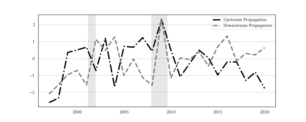
(a)

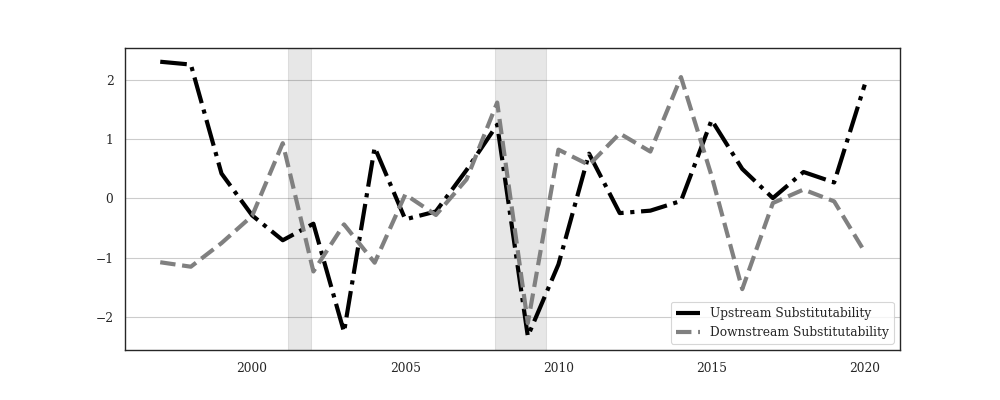
(b)

Figure 1: Network Propagation Risk Factors

Notes: This figure plots the time series of network propagation risk factors (Panel A), the cross-sectional average industry substitutability (Panel B). Shaded regions indicate NBER-dated recession periods.

5.2 Asset Pricing Tests

To verify the prices of risk predicted in (17), I sort stocks based on their exposure to factors and form quintile-sorted portfolios. In particular, for every stock $\color[rgb]{0,0,0}i$ I regress annual excess returns $\color[rgb]{0,0,0}r_{it}-r_{ft}$ on a constant, aggregate demand and productivity growth, and additional controls. The main regression is given by:

$$\color[rgb]{0,0,0}\displaystyle r_{it}-r_{ft}=\alpha_{i}+\beta_{ia}a_{t}+\beta_{ig}g_{t}+\beta_{iu}W_{ut}+\beta_{id}W_{dt}+\varepsilon_{it},$$ (23)

where equation (17) implies that stocks with high $\color[rgb]{0,0,0}\beta_{ia}$ and $\color[rgb]{0,0,0}\beta_{ig}$ should have higher expected excess returns and stocks with high $\color[rgb]{0,0,0}\beta_{iu}$ and $\color[rgb]{0,0,0}\beta_{id}$ should have lower expected excess returns. For each year $\color[rgb]{0,0,0}t$, I compute stock exposure to factors on a 15-year rolling window from $\color[rgb]{0,0,0}t-14$ to $\color[rgb]{0,0,0}t$ using (23), and then sort stocks into five portfolios on each beta both separately (one-way sort) and pairwise (two-way sort). Then I construct value and equal-weighted portfolios over the subsequent year $\color[rgb]{0,0,0}t+1$ and compute average out-of-sample excess returns for each portfolio.

Table 4 provides evidence of a significant return spread in one-way beta sorted portfolios. In particular, the highest quintile upstream propagation beta portfolio earns -11.42% lower annual returns than the lowest quintile portfolio, while the highest quintile downstream propagation beta portfolio earns -4.18% lower annual returns than the lowest quintile portfolio. Both return spreads are statistically significant, although more pronounced for upstream propagation beta sorted portfolios. This is consistent with Herskovic et al. (2020b), who argue that upstream propagation is the more important channel.

I also observe a return spread in post-sample alphas from the CAPM and Fama and French (FF3) three factor models, which implies that network propagation risk is not captured by market returns or FF3 factors. In light of the variance results of Section 3, I also verify that return spreads are not explained by market volatility or idiosyncratic volatility factors in Table 17. Additionally, return spreads cannot be explained by differences in return volatility, average size, or average book-to-market ratios. Finally, the average correlation between upstream and downstream propagation betas is 8.6%, suggesting that the two network factors are distinct sources of risk.

Return spreads are robust to the choice of trailing window length, equal or value weighting in portfolios, control variables, and show up in double-sorted portfolios as well. See Appendix H for more details.

Table 4: One-Way Sorted Portfolios on Network Propagation Factors

Panel A: One-way sorts on upstream propagation beta (controlling for $\color[rgb]{0,0,0}a_{t}$ and $\color[rgb]{0,0,0}g_{t}$)
	1 (Low)	2	3	4	5 (High)	H-L	t(H-L)	MR p-val
$\color[rgb]{0,0,0}\mathbb{E}[r]-r_{f}$	18.10	12.81	10.59	9.42	6.69	-11.42	-13.22	0.07
$\color[rgb]{0,0,0}\alpha_{capm}$	0.29	-0.1	-0.23	-0.31	-1.02	-1.32	-15.71	0.05
$\color[rgb]{0,0,0}\alpha_{ff3}$	0.08	-0.09	-0.22	-0.29	-0.54	-0.63	-8.61	0.09
Volatility (%)	15.54	13.89	13.59	13.03	19.66	-	-	-
Book-to-market	0.52	0.56	0.53	0.55	0.50	-	-	-
Market value ($bn)	6.46	16.99	10.62	15.15	9.11	-	-	-
Panel B: One-way sorts on downstream propagation beta (controlling for $\color[rgb]{0,0,0}a_{t}$ and $\color[rgb]{0,0,0}g_{t}$)
	1 (Low)	2	3	4	5 (High)	H-L	t(H-L)	MR p-val
$\color[rgb]{0,0,0}\mathbb{E}[r]-r_{f}$	13.54	13.23	11.02	9.77	9.36	-4.18	-7.56	0.25
$\color[rgb]{0,0,0}\alpha_{capm}$	-0.04	-0.18	-0.28	-0.38	-0.60	-0.56	-4.78	0.00
$\color[rgb]{0,0,0}\alpha_{ff3}$	-0.11	-0.14	-0.23	-0.28	-0.36	-0.25	-3.62	0.03
Volatility (%)	15.44	13.95	18.58	12.99	13.88	-	-	-
Book-to-market	0.52	0.56	0.55	0.53	0.51	-	-	-
Market value ($bn)	15.84	7.45	4.54	17.6	12.72	-	-	-
Panel C: One-way sorts on upstream propagation beta (no controls)
	1 (Low)	2	3	4	5 (High)	H-L	t(H-L)	MR p-val
$\color[rgb]{0,0,0}\mathbb{E}[r]-r_{f}$	15.15	12.61	11.46	9.44	7.23	-7.91	-11.57	0.07
$\color[rgb]{0,0,0}\alpha_{capm}$	0.09	-0.15	-0.17	-0.28	-1.09	-1.18	-17.53	0.26
$\color[rgb]{0,0,0}\alpha_{ff3}$	-0.12	-0.14	-0.18	-0.22	-0.58	-0.46	-9.96	0.31
Volatility (%)	15.26	14.23	13.57	12.61	20.97	-	-	-
Book-to-market	0.54	0.58	0.52	0.52	0.50	-	-	-
Market value ($bn)	6.87	17.48	10.92	16.38	6.56	-	-	-
Panel D: One-way sorts on downstream propagation beta (no controls)
	1 (Low)	2	3	4	5 (High)	H-L	t(H-L)	MR p-val
$\color[rgb]{0,0,0}\mathbb{E}[r]-r_{f}$	12.66	11.94	11.8	8.34	5.13	-7.53	-8.65	0.42
$\color[rgb]{0,0,0}\alpha_{capm}$	-0.15	-0.18	-0.19	-0.4	-0.64	-0.49	-11.37	0.41
$\color[rgb]{0,0,0}\alpha_{ff3}$	-0.10	-0.21	-0.21	-0.29	-0.32	-0.22	-4.76	0.44
Volatility (%)	14.09	13.9	14.44	13.22	31.95	-	-	-
Book-to-market	0.54	0.49	0.58	0.51	0.54	-	-	-
Market value ($bn)	15.97	12.79	6.33	16.88	6.34	-	-	-

Notes: This table reports average excess returns and post-sample alphas in annual percentages for value-weighted portfolios sorted into quintiles on annual upstream and downstream propagation factors. Sample is between 1997-2021 for more than 10,000 stocks belonging to the BEA 66 non-government industry classifications. Panels A and B control for productivity growth and federal procurement demand growth, while Panels C and D have no controls. I also report average return volatility, book-to-market ratio and market value for each portfolio. To test for significant return spreads, I report $\color[rgb]{0,0,0}t$-statistics for the null hypothesis $\color[rgb]{0,0,0}H_{0}:xr_{5}=xr_{1}$, where $\color[rgb]{0,0,0}xr_{q}$ is the average return of the $\color[rgb]{0,0,0}q^{th}$ quintile single sorted portfolio. Moreover, I report p-values for the test $\color[rgb]{0,0,0}H_{0}:xr_{q+1}<xr_{q}\forall q\leq 4$, calculated via bootstrap following Patton and Timmermann (2010).

5.3 Verifying Macroeconomic Predictions

Equation (16) predicts that upstream and downstream propagation factors should be negatively correlated with consumption, output growth, and aggregate dividend growth. To test this, I construct aggregate series between 1997-2021 for consumption and output growth from the National Income and Product Accounts (NIPA) and corporate dividend growth from BEA data. Then I regress each outcome on network propagation factors, controlling for aggregate productivity and federal procurement demand growth. I standardize each variable to have zero mean and unit standard deviation. Consistent with the predictions of the model, Table 5 reports negative and statistically significant coefficients on both upstream and downstream propagation risk factors. The factors explain a large portion of time variation in consumption, output, and dividend growth with $\color[rgb]{0,0,0}R^{2}$ values of 56%, 68%, and 26%, respectively.

The coefficients on downstream propagation are -0.17 ($\color[rgb]{0,0,0}t=-1.89$), -0.60 ($\color[rgb]{0,0,0}t=-2.57$), and -0.01 ($\color[rgb]{0,0,0}t=-0.52$) for aggregate consumption, output, and dividend growth regressions, respectively. On the other hand, the coefficients on upstream propagation are not significant for aggregate consumption and output growth regressions, although the coefficient in the dividend growth regression is $\color[rgb]{0,0,0}-0.03$ ($\color[rgb]{0,0,0}t=-1.80$). Additionally, the coefficients on upstream propagation are significant when the dependent variable is limited to only durable consumption or output growth, -0.111 ($\color[rgb]{0,0,0}t=-2.39$) and -1.38 ($\color[rgb]{0,0,0}t=-2.39$), respectively. This suggests that durable consumption is more sensitive to upstream (supply-side) risk.

Table 5: Network Propagation and Macroeconomic Factors

Variable	$\color[rgb]{0,0,0}\Delta c_{t}$	$\color[rgb]{0,0,0}\Delta c_{t}^{dur}$	$\color[rgb]{0,0,0}\Delta c_{t}^{nondur}$	$\color[rgb]{0,0,0}\Delta y_{t}$	$\color[rgb]{0,0,0}\Delta y_{t}^{dur}$	$\color[rgb]{0,0,0}\Delta y_{t}^{nondur}$	$\color[rgb]{0,0,0}\Delta D_{t}$
$\color[rgb]{0,0,0}W_{ut}$	0.003	-0.111**	-0.158	-0.112	-1.383**	-0.416	-0.033*
	(0.103)	(0.048)	(0.087)	(0.275)	(0.607)	(0.229)	(0.021)
$\color[rgb]{0,0,0}W_{dt}$	-0.174*	-0.031	-0.022	-0.598**	-0.387	-0.058	-0.010
	(0.074)	(0.054)	(0.101)	(0.222)	(0.684)	(0.267)	(0.021)
$\color[rgb]{0,0,0}a_{t}$	0.321**	0.128**	0.197**	1.018**	1.607**	0.520**	0.018
	(0.114)	(0.055)	(0.108)	(0.271)	(0.689)	(0.285)	(0.010)
$\color[rgb]{0,0,0}g_{t}$	0.271	-0.056	0.604	-0.011	-0.704	1.592	0.029
	(0.332)	(0.276)	(0.638)	(0.956)	(3.450)	(1.682)	(0.109)
Intercept	-0.485	-0.111	-0.205	1.218	4.09	2.023	0.042
Obs	24	24	24	24	24	24	24
$\color[rgb]{0,0,0}R^{2}$	0.56	0.537	0.376	0.679	0.537	0.376	0.257

Notes: This table reports results of OLS regressions of aggregate consumption growth, output growth, and dividend growth on input-output network propagation risk factors, controlling for productivity and federal procurement demand growth. The columns represent different dependent variables corresponding to aggregate PCE growth, durable consumption growth, non-durable consumption growth, output growth, durable output growth, non-durable output growth, and dividend growth. All series are standardized to have zero mean and unit variance. Sample is at an annual frequency between 1997-2021.

6 Conclusion

In this work, I propose a production-based asset pricing model with input-output networks in which productivity shocks propagate downstream from suppliers to customers and demand shocks propagate upstream from customers to suppliers. This model is consistent with a benchmark reduced-form equation that links output growth of each node (industry or firm) in the network to output growth of other nodes and a node-specific shock. Almost all research in this area assumes that node-specific shocks are idiosyncratic- that is, drawn independently across units. In this work, I prove that the idiosyncratic shock assumption in this reduced-form equation is not consistent with realistic input-output networks. I argue that researchers who make use of network models should account for potential inter-node correlation in propagated shocks.

When accounting for non-negligible correlation in shocks, the variance expression for output growth gains an additional component which depends on a weighted sum of covariances of shocks between each node’s trade partners. As a result, units in the network are exposed to risk associated with the homogeneity of their customer and supplier connections. This generates cross-sectional differences in nodes’ ability to substitute away from correlated shocks propagating through the network. I define substitutability as the negative value of the new covariance term, termed concentration “between” suppliers. Consistent with theory, I provide empirical evidence that customer and supplier substitutability can explain differences in realized variance across industries. In particular, higher substitutability (lower between-concentration) explains lower realized variance, conditional on other input-output and variance related characteristics.

Although the covariance between shocks is defined in a purely statistical sense, I also investigate industry characteristics which can provide a structural explanation for high correlation in shocks. To this end, I argue that technological proximity explains correlation in supply-side shocks that propagate downstream, while product similarity explains correlation in demand-side shocks that propagate upstream. As a result, supply chain substitutability can be calculated as a function of distances between units in latent technology and product space. Although there is evidence of other sources of correlation in shocks, this simplification is simple, tractable, and can be incorporated in theoretical models to provide a structural origin for correlation in shocks.

I incorporate this mechanism in an extension of the network model which directly models the propagation of shocks between firms in the input-output network. The propensity that shocks propagate is a decreasing function in substitutability, such that firms with more substitutable supply chains are less likely to experience shocks. Moreover, demand shock substitutability is captured by network-weighted dispersion of a firm’s customers in latent product space, while supply shock substitutability is captured by network-weighted dispersion of a firm’s suppliers in latent technology space. In the extended model, systematic risk is driven by the average propagation of upstream and downstream transmitted shocks.

Under some reasonable assumptions, I calibrate the model to data on publicly traded firms and construct empirical analogues of upstream and downstream propagation risk factors. I provide evidence that these risk factors are negatively priced in the cross-section of returns. Additionally, consistent with the model’s theoretical predictions, both factors are associated with lower aggregate consumption growth, lower output growth, and lower dividend growth. Empirical results suggest the importance of both directions of propagation as significant sources of systematic risk in the economy.

Future work might investigate in more depth the sources of correlation in supply and demand shocks and generate more granular estimates of the agents’ ability to substitute away from them.

Appendix A General Equilibrium Model of Input-Output Linkages

In this section, I show that (1) can be cast as an outcome of a production-based asset pricing model. This model provides a structural foundation for the theoretical contributions of this work and is closely related to Acemoglu et al. (2012), Acemoglu et al. (2016), Ramìrez (2017), and Herskovic (2018b). Consider a competitive economy with $\color[rgb]{0,0,0}n$ production units (firms or industries) with Cobb-Douglas technology, representative households with constant relative risk aversion (CRRA) preferences over a basket of goods and who work and own shares in all firms and live off wages and dividends, and a government that finances purchases with a lump-sum tax. In this economy, Hicks-neutral productivity shocks propagate downstream from suppliers to customers, while government demand shocks propagate upstream from customers to suppliers.

A.1 Production

Production unit $\color[rgb]{0,0,0}i$’s output is a constant returns to scale function of labor and intermediate inputs:

$$\color[rgb]{0,0,0}\displaystyle y_{it}=\exp(z_{it})\ell_{it}^{\alpha_{i\ell}}\prod_{j=1}^{n}x_{ijt}^{w_{ijt}},$$ (24)

where $\color[rgb]{0,0,0}x_{ijt}$ is the amount of product $\color[rgb]{0,0,0}j$ used as input by industry $\color[rgb]{0,0,0}i$ at time $\color[rgb]{0,0,0}t$, $\color[rgb]{0,0,0}\ell_{it}$ is labor input, and $\color[rgb]{0,0,0}z_{it}$ is a Hicks-neural productivity shock, respectively. I assume that for all $\color[rgb]{0,0,0}i$ and $\color[rgb]{0,0,0}t$, the labor share of production is positive (i.e., $\color[rgb]{0,0,0}\alpha_{i\ell}>0$) and intermediate input shares are non-negative ($\color[rgb]{0,0,0}w_{ijt}\geq 0$) and sum to the capital share of production (i.e., ($\color[rgb]{0,0,0}\sum_{j=1}^{n}w_{ijt}=1-\alpha_{i\ell}$).

Taking both spot market prices and input shares as given, production units optimize dividends (denoted $\color[rgb]{0,0,0}D_{it}$) as a function of input and labor purchases:

$$\color[rgb]{0,0,0}\displaystyle D_{it}=\max_{\{x_{ijt}\}_{j=1}^{n},\ell_{it}}p_{it}y_{it}-\sum_{j=1}^{n}p_{jt}x_{ijt}-p_{wt}\ell_{it}$$ (25)

subject to (24) and $\color[rgb]{0,0,0}\ell_{it}\in(0,1)$. Suppose further that $\color[rgb]{0,0,0}M_{t+1}$ is the stochastic discount factor (SDF) that prices all assets in the economy. Then the cum dividend value of firm $\color[rgb]{0,0,0}i$ (denoted $\color[rgb]{0,0,0}V_{it}$) satisfies the following Bellman equation:

$$\color[rgb]{0,0,0}\displaystyle V_{it}=D_{it}+\mathbb{E}_{t}[M_{t+1}V_{i,t+1}].$$ (26)

A.2 Government

The government purchases goods $\color[rgb]{0,0,0}G_{it}$ from each unit $\color[rgb]{0,0,0}i$ at time $\color[rgb]{0,0,0}t$ and finances them via a lump-sum tax $\color[rgb]{0,0,0}T_{t}$. Taking prices as given, the government’s financing constraint implies that $\color[rgb]{0,0,0}T_{t}=\sum_{i=1}^{n}p_{it}G_{it}$.

A.3 Households

Assume that the representative household owns shares in each unit and has the following preferences:

$$\color[rgb]{0,0,0}\displaystyle u(c_{1t},...,c_{nt},\ell)=\frac{1}{1-\gamma}\cdot\bigg{(}\prod_{i=1}^{n}c_{it}^{\beta_{i}}\bigg{)}^{1-\gamma}\cdot g(\ell_{t}),$$ (27)

where $\color[rgb]{0,0,0}c_{it}$ is the consumption of good $\color[rgb]{0,0,0}i$ with preference weights $\color[rgb]{0,0,0}\beta_{i}$ such that $\color[rgb]{0,0,0}\sum_{i}\beta_{i}$ = 1 and $\color[rgb]{0,0,0}g(.)=(1-\ell_{t})^{\nu}$ is a decreasing and differentiable function capturing disutility of labor. Households also have a time-discount factor of $\color[rgb]{0,0,0}\beta$ and cannot store goods from one period to another. In equilibrium, households hold a zero net position in a risk-free asset and choose to own $\color[rgb]{0,0,0}\vartheta_{it}$ in each unit according to the following budget constraint:

$$\color[rgb]{0,0,0}\displaystyle T_{t}+p_{wt}\ell_{t}+\sum_{i=1}^{n}p_{it}c_{it}+\sum_{i=1}^{n}\vartheta_{i,t+1}(V_{it}-D_{it})=\sum_{i=1}^{n}\vartheta_{i,t}V_{it},$$ (28)

where the right hand side is total value of investments and the left hand side is the sum of taxes paid, wages earned, cost of consumption, and unrealized capital gains, respectively. The household’s optimization problem satisfies the Bellman equation:

$$\color[rgb]{0,0,0}\displaystyle U_{t}=\max_{\{c_{it},\vartheta_{i,t+1},\ell\}_{i=1}^{n}}u(.)+\beta\mathbb{E}_{t}[U_{t+1}],$$ (29)

subject to (28).

A.4 Equilibrium

The competitive equilibrium of the economy consists of spot market prices $\color[rgb]{0,0,0}\{p_{it}\}_{i=1}^{n}$, consumption bundles $\color[rgb]{0,0,0}\{c_{it}\}_{i=1}^{n}$, share holdings $\color[rgb]{0,0,0}\{\vartheta_{it}\}_{i=1}^{n}$, labor supply $\color[rgb]{0,0,0}\ell_{t}$, wages $\color[rgb]{0,0,0}p_{wt}$, and input bundles $\color[rgb]{0,0,0}\{x_{ijt}\}_{i,j=1}^{n}$ such that both production units and households exhibit optimal behavior and good/asset markets clear.

A.4.1 Market Clearing

In equilibrium, all good markets clear such that:

$$\color[rgb]{0,0,0}\displaystyle y_{it}=\underbrace{c_{it}}_{\text{final consumption demand}}+\underbrace{\sum_{j=1}^{n}x_{jit}}_{\text{intermediate demand}}+\underbrace{G_{it}}_{\text{government consumption}},$$

and all asset markets clear $\color[rgb]{0,0,0}\vartheta_{it}=1$ for all $\color[rgb]{0,0,0}i$ and $\color[rgb]{0,0,0}t$.

A.4.2 Producer Optimality

Taking prices as given, unit $\color[rgb]{0,0,0}i$’s first order dividend maximizing conditions satisfy

$$\color[rgb]{0,0,0}\displaystyle w_{ijt}=\frac{p_{jt}x_{ijt}}{p_{it}y_{it}}\equiv\frac{sales_{j\to i}}{sales_{i}}$$ (30)

and

$$\color[rgb]{0,0,0}\displaystyle\alpha_{i\ell}=\frac{p_{wt}\ell_{it}}{p_{it}y_{it}}$$ (31)

A.4.3 Consumer Optimality

Given the Cobb-Douglas aggregation in preferences over goods (i.e., $\color[rgb]{0,0,0}C_{t}:=\prod_{i}c_{it}^{\beta_{i}}$), utility maximizing households consume $\color[rgb]{0,0,0}\beta_{i}$ of income on good $\color[rgb]{0,0,0}i$ and hold shares fixed at $\color[rgb]{0,0,0}\vartheta_{it}=1$. More specifically, letting $\color[rgb]{0,0,0}\lambda_{t}$ be the Lagrange multiplier for the period $\color[rgb]{0,0,0}t$ household budget constraint, the first-order condition for consumption is written:

$$\color[rgb]{0,0,0}\displaystyle\lambda_{t}=\frac{C_{t}^{-\gamma}}{p_{it}}\cdot\frac{\partial C_{t}}{\partial c_{it}}.$$ (32)

This implies that equilibrium consumption satisfies:

$$\color[rgb]{0,0,0}\displaystyle p_{it}c_{it}=\beta_{i}\bigg{(}p_{wt}\ell_{t}^{*}+\sum_{j=1}^{n}D_{jt}-T_{t}\bigg{)}.$$ (33)

where $\color[rgb]{0,0,0}\ell_{t}^{*}$ solves:

$$\color[rgb]{0,0,0}\displaystyle\frac{p_{wt}\ell_{t}^{*}}{p_{wt}\ell_{t}^{*}+\sum_{j=1}^{n}D_{jt}-T_{t}}=-\frac{\ell_{t}^{*}g^{\prime}(\ell_{t}^{*})}{g(\ell_{t}^{*})}$$ (34)

A.4.4 Asset Prices

From (32), the stochastic discount factor can be written:

$$\color[rgb]{0,0,0}\displaystyle M_{t+1}=\beta\frac{\lambda_{t+1}}{\lambda_{t}}=\beta\bigg{(}\frac{C_{t+1}}{C_{t}}\bigg{)}^{-\gamma}\frac{p_{it}\cdot\partial C_{t+1}/\partial c_{i,t+1}}{p_{i,t+1}\cdot\partial C_{t}/\partial c_{it}}.$$ (35)

Following Herskovic (2018a), I assume that prices are normalized such that $\color[rgb]{0,0,0}p_{it}=\partial C_{t}/\partial c_{it}$, or equivalently that $\color[rgb]{0,0,0}\prod_{j}p_{jt}^{\beta_{j}}=\prod_{j}\beta_{j}^{\beta_{j}}$ for all $\color[rgb]{0,0,0}i$ and $\color[rgb]{0,0,0}t$. This implies the the utility aggregator is equal to the household’s consumption expenditure $\color[rgb]{0,0,0}C_{t}=\sum_{i=1}^{n}p_{it}c_{it}$.. Then (35) simplifies to:

$$\color[rgb]{0,0,0}\displaystyle M_{t+1}=\beta\bigg{(}\frac{\sum_{i=1}^{n}p_{i,t+1}c_{i,t+1}}{\sum_{i=1}^{n}p_{it}c_{it}}\bigg{)}^{-\gamma}.$$ (36)

A.4.5 Shock Propagation

I now derive closed form expressions for the effects of productivity and government demand shocks on output growth in this model. The main takeaway is that output growth is captured by the following reduced form expression:

$$\color[rgb]{0,0,0}\displaystyle\mathbf{d}\log\mathbf{y}_{t}=\mathbf{H}_{down,t}\mathbf{dz}_{t}+\mathbf{H}_{up,t}\mathbf{dG}_{t},$$

where $\color[rgb]{0,0,0}\mathbf{H}_{.,t}$ are $\color[rgb]{0,0,0}n\times n$ Leontief inverse propagation matrices. I provide a derivation for each component separately.

Productivity Shocks

Totally differentiate the expression in (24) to obtain:

$$\color[rgb]{0,0,0}\displaystyle d\log y_{it}=dz_{it}+\alpha_{i\ell}d\log\ell_{it}+\sum_{j=1}^{n}w_{ijt}d\log x_{ijt}$$ (37)

Totally differentiating (30), (31), and (33) and plugging in to this expression yields:

$$\color[rgb]{0,0,0}\displaystyle d\log y_{it} \color[rgb]{0,0,0}\displaystyle=dz_{it}+\alpha_{i\ell}d\log\ell_{it}+\sum_{j=1}^{n}w_{ijt}(d\log y_{it}+d\log p_{it}-d\log p_{jt})$$

$$\color[rgb]{0,0,0}\displaystyle=dz_{it}+\alpha_{i\ell}(d\log y_{it}-d\log c_{it})+\sum_{j=1}^{n}w_{ijt}(d\log y_{it}-d\log c_{it}+d\log c_{jt}).$$

Given constant returns to scale ($\color[rgb]{0,0,0}\alpha_{i\ell}+\sum_{j}w_{ij}=1$), this expression can be further simplified as follows:

$$\color[rgb]{0,0,0}\displaystyle d\log c_{i}=dz_{it}+\sum_{j=1}^{n}w_{ijt}d\log c_{j}$$

or in vector notation:

$$\color[rgb]{0,0,0}\displaystyle\mathbf{d}\log\mathbf{c}_{t}=\mathbf{dz}_{t}+\mathbf{W}_{t}\mathbf{d}\log\mathbf{c}_{t},$$

where $\color[rgb]{0,0,0}\mathbf{W}_{t}$ has entries $\color[rgb]{0,0,0}w_{ijt}$. Note that market clearing and profit maximization conditions together imply that:

$$\color[rgb]{0,0,0}\displaystyle\frac{y_{jt}}{c_{jt}}=1+\sum_{i=1}^{n}w_{ijt}\frac{\beta_{i}y_{it}}{\beta_{j}c_{it}}$$

which implies that equilibrium consumption growth is equal to equilibrium output growth:

$$\color[rgb]{0,0,0}\displaystyle\mathbf{d}\log\mathbf{c}_{t}=\mathbf{d}\log\mathbf{y}_{t}$$ (38)

and thus that:

$$\color[rgb]{0,0,0}\displaystyle\mathbf{d}\log\mathbf{y}_{t}=(\mathbf{I}-\mathbf{W}_{t})^{-1}\mathbf{dz}_{t},$$ (39)

where $\color[rgb]{0,0,0}\mathbf{H}_{down,t}:=(\mathbf{I}-\mathbf{W}_{t})^{-1}$ is the Leontief inverse of $\color[rgb]{0,0,0}\mathbf{W}_{t}$. Here, the $\color[rgb]{0,0,0}\mathbf{W}_{t}$ matrix determines the strength of downstream propagation of productivity shocks.

Demand Shocks

To study the effects of government spending shocks in the model, normalize $\color[rgb]{0,0,0}\mathbf{z}_{t}=0$ and consider the unit cost function for $\color[rgb]{0,0,0}i$:

$$\color[rgb]{0,0,0}\displaystyle C_{it}(\mathbf{p}_{t},p_{wt})=A_{it}p_{wt}^{\alpha_{i\ell}}\prod_{j=1}^{n}p_{jt}^{w_{ijt}},\quad\text{where }A_{it}=\alpha_{i\ell}^{-\alpha_{i\ell}}\prod_{j=1}^{n}w_{ijt}^{-w_{ijt}}.$$

The zero productivity normalization implies zero dividends for production units, and combined with the price normalization for wages, this implies that:

$$\color[rgb]{0,0,0}\displaystyle\log p_{it}=\log A_{it}+\sum_{j=1}^{n}w_{ijt}\log p_{jt}$$

Conditional on productivity vector $\color[rgb]{0,0,0}\mathbf{z}_{t}$ and defining the vector $\color[rgb]{0,0,0}\mathbf{a}_{t}$ with entries $\color[rgb]{0,0,0}\log A_{it}$, prices are a function of the network and cost but not government purchases:

$$\color[rgb]{0,0,0}\displaystyle\log\mathbf{p}_{t}=(\mathbf{I}-\mathbf{W}_{t})^{-1}\mathbf{a}_{t}.$$

Setting $\color[rgb]{0,0,0}\nu=1$ Then (34) and the fact that $\color[rgb]{0,0,0}T_{t}=\sum_{i}p_{it}G_{it}$ implies that:

$$\color[rgb]{0,0,0}\displaystyle\ell_{t}=\frac{1}{2}+\frac{1}{2}\sum_{i=1}^{n}p_{it}G_{it}$$ (40)

and thus:

$$\color[rgb]{0,0,0}\displaystyle p_{it}c_{it}=\beta_{i}[p_{wt}\ell_{t}-T_{t}]=\frac{\beta_{i}}{2}\bigg{(}1-\sum_{j=1}^{n}p_{jt}G_{jt}\bigg{)}.$$

Differentiating and combining with the resource constraint and profit maximization conditions yields:

$$\color[rgb]{0,0,0}\displaystyle\frac{d(p_{it}y_{it})}{p_{it}y_{it}}=\sum_{j=1}^{n}w_{jit}\frac{d(p_{jt}y_{jt}}{p_{it}y_{it}}+\frac{dG_{it}}{y_{it}}-\frac{\beta_{i}}{2}\sum_{j=1}^{n}\frac{d(p_{jt}G_{jt})}{p_{it}y_{it}}.$$

Since prices are constant (i.e., $\color[rgb]{0,0,0}d(p_{it}y_{it})/p_{it}y_{it}=d\log y_{it}$), I can write in vector notation:

$$\color[rgb]{0,0,0}\displaystyle\mathbf{d}\log\mathbf{y}_{t}=\mathbf{H}_{up,t}\mathbf{dG_{t}},$$ (41)

where $\color[rgb]{0,0,0}\mathbf{H}_{up,t}=(\mathbf{I}-\mathbf{W}_{t}^{\top})^{-1}\mathbf{\Lambda}_{t}$ is the upstream propagation Leontief inverse and $\color[rgb]{0,0,0}\mathbf{\Lambda}_{t}$ is a scaling matrix with diagonal entries $\color[rgb]{0,0,0}(1-\beta_{i}/2)/p_{it}y_{it}$ and off-diagonal entries $\color[rgb]{0,0,0}-(\beta_{i}/2)/p_{it}y_{it}$ for row indices $\color[rgb]{0,0,0}i$.

Appendix B Product Varieties in Latent Space

Suppose that each industry (or firm) is associated with a random position $\color[rgb]{0,0,0}z_{it}:=(\cos\theta_{it},\sin\theta_{it})$ on a circular surface on the $\color[rgb]{0,0,0}3$-dimensional hypersphere $\color[rgb]{0,0,0}\mathcal{S}^{p+1}$. Suppose that the surface represents the space of varieties in production technology space. I also assume each unit corresponds to a position in latent product variety space, and that product positions are independent of technological positions. The stochastic process for positions is the same in both spaces and depends on changes in the angle $\color[rgb]{0,0,0}\theta_{it}$ as follows:

$$\color[rgb]{0,0,0}\displaystyle\theta_{it}=\rho\cdot\theta_{i,t-1}+\epsilon_{it},\qquad\epsilon_{it}\sim_{iid}\mathcal{N}(0,\sigma_{\theta}^{2}),$$ (42)

where $\color[rgb]{0,0,0}\theta_{it}$ is measured in radians. The distance between two points $\color[rgb]{0,0,0}i$ and $\color[rgb]{0,0,0}j$ can then be written:

$$\color[rgb]{0,0,0}\displaystyle\delta_{ijt}=\frac{1}{2\pi}|\theta_{it}-\theta_{jt}|.$$ (43)

This implies a correlation structure in the distances between units as follows:

$$\color[rgb]{0,0,0}\displaystyle\text{corr}(\delta_{ijt},\delta_{kmt})=\begin{cases}0&\text{if }i\notin\{k,m\}\cap j\notin\{k,m\},\\ 1&\text{if }i\in\{k,m\}\cup j\in\{k,m\},\end{cases},$$ (44)

or equivalently that:

$$\color[rgb]{0,0,0}\displaystyle\text{cov}(\delta_{ijt},\delta_{kmt})=\begin{cases}0&\text{if }i\notin\{k,m\}\cap j\notin\{k,m\},\\ \sqrt{\text{var}(\delta_{ijt})\text{var}(\delta_{kmt})}&\text{if }i\in\{k,m\}\cup j\in\{k,m\},\end{cases},$$ (45)

where:

$$\color[rgb]{0,0,0}\displaystyle\sigma_{d}^{2}:=\text{var}(\delta_{ijt}) \color[rgb]{0,0,0}\displaystyle=\text{var}(\theta_{it})+\text{var}(\theta_{jt})-\mathbb{E}[|\theta_{it}-\theta_{jt}|]^{2}=\frac{2\sigma_{\theta}^{2}}{1-\varphi^{2}}-\frac{(4/\pi)\sigma_{\theta}^{2}}{1-\varphi^{2}},$$

Define the set of $\color[rgb]{0,0,0}i$’s $\color[rgb]{0,0,0}q$-stream located trade partners by $\color[rgb]{0,0,0}A_{iqt}:=\{k:A_{ki}(\mathcal{G}_{qt})\neq\emptyset\}$. Note that in technology space, $\color[rgb]{0,0,0}q$ refers to upstream propagation. Combining with equation (14) yields:

$$\color[rgb]{0,0,0}\displaystyle\text{cov}(s_{iqt},s_{jqt}) \color[rgb]{0,0,0}\displaystyle=\sum_{k\neq\ell}\sum_{m\neq p}w_{ikt}w_{i\ell t}w_{jmt}w_{jpt}\cdot\text{cov}(\delta_{k\ell t},\delta_{mpt})$$

$$\color[rgb]{0,0,0}\displaystyle=\sum_{k,\ell\in A_{iqt};m,p\in A_{jqt}}w_{ikt}w_{i\ell t}w_{jmt}w_{jpt}\cdot\sigma_{d}^{2}\cdot\mathbbm{1}\{(m\in A_{iqt})\cup(p\in A_{iqt})\}$$

Additionally, $\color[rgb]{0,0,0}s_{iqt}$ are jointly distributed as a folded truncated normal with variance-covariance matrix $\color[rgb]{0,0,0}\mathbf{\Sigma}_{qt}=[\text{cov}(s_{iqt},s_{jqt})]_{ij}$ and mean vector $\color[rgb]{0,0,0}\boldsymbol{\mu}_{qt}=[\mu_{iqt}]_{i}$ with entries:

$$\color[rgb]{0,0,0}\displaystyle\mu_{iqt}:=\mathbb{E}[s_{iqt}] \color[rgb]{0,0,0}\displaystyle=-\sigma_{d}\sqrt{8/\pi}\cdot\sum_{j<k;j,k\in A_{iqt}}w_{ijt}w_{ikt}.$$

When $\color[rgb]{0,0,0}i=j$, I can further simplify as follows:

$$\color[rgb]{0,0,0}\displaystyle\text{var}(s_{iqt}) \color[rgb]{0,0,0}\displaystyle=4\sigma_{d}^{2}\cdot\sum_{j<k;j,k\in A_{iqt}}(w_{ijt}w_{ikt})^{2}.$$

Next, using equation (13), I can write the log-odds function as follows:

$$\color[rgb]{0,0,0}\displaystyle l_{iqt}:=\log\bigg{(}\frac{p_{iqt}}{1-p_{iqt}}\bigg{)} \color[rgb]{0,0,0}\displaystyle=k\bigg{(}s_{iqt}-\frac{1}{n}\sum_{i=1}^{n}s_{iqt}\bigg{)}=k\bigg{(}\hat{e}_{in}^{\top}-\frac{1}{n}\iota_{n}^{\top}\bigg{)}\mathbf{s}_{qt},$$

where $\color[rgb]{0,0,0}\hat{e}_{in}$ is the $\color[rgb]{0,0,0}i$th column of an $\color[rgb]{0,0,0}n\times n$ identity matrix and $\color[rgb]{0,0,0}\iota_{n}$ is an $\color[rgb]{0,0,0}n\times 1$ vector of ones. Equivalently, the vector $\color[rgb]{0,0,0}\mathbf{l}_{qt}:=(l_{1qt},...,l_{nqt})^{\top}$ can be written:

$$\color[rgb]{0,0,0}\displaystyle\mathbf{l}_{qt} \color[rgb]{0,0,0}\displaystyle=k\bigg{(}\mathbf{I}_{n}-\frac{\iota_{n}\iota_{n}^{\top}}{n}\bigg{)}\mathbf{s}_{qt}\sim\mathcal{N}\big{(}\mathbf{B}_{k,n}\boldsymbol{\mu}_{qt},\mathbf{B}_{k,n}^{\top}\mathbf{\Sigma}_{qt}\mathbf{B}_{k,n}\big{)},$$

where $\color[rgb]{0,0,0}\mathbf{B}_{k,n}:=k(\mathbf{I}_{n}-\iota_{n}\iota_{n}^{\top}/n)$. Notice that $\color[rgb]{0,0,0}p_{iqt}=F(l_{iqt})$ where $\color[rgb]{0,0,0}F(x)=(1+\exp(-x))^{-1}$ and thus the vector $\color[rgb]{0,0,0}\mathbf{p}_{qt}$ has a logistic normal distribution and thus no closed form representation for its mean vector and variance-covariance matrix. However, I can write $\color[rgb]{0,0,0}\text{median}(\mathbf{p}_{qt})=F(\mathbf{B}_{k,n}\boldsymbol{\mu}_{qt})$.

Appendix C Proofs

C.1 Proof of Proposition 2.3

I begin by characterizing the family of matrices $\color[rgb]{0,0,0}\mathbf{W}\in M_{n}$ that are consistent with Assumptions 2.1 and 2.2 with a sequence of if and only if relationships. First define $\color[rgb]{0,0,0}\mathbf{\Sigma}_{y}:=\mathbb{V}[\mathbf{y}]$ to be the variance-covariance matrix of sectoral production, and notice that Assumption 2.2 implies that $\color[rgb]{0,0,0}\mathbf{\Sigma}_{y}=(\mathbf{I}-\mathbf{W})^{-1}\mathbf{D}(\mathbf{I}-\mathbf{W}^{\top})^{-1}$ is non-negative. This is because $\color[rgb]{0,0,0}\mathbf{\Sigma}_{y}$ is the product of non-negative matrices by definition since $\color[rgb]{0,0,0}(\mathbf{I}-\mathbf{W})^{-1}=\mathbf{I}+\mathbf{W}+\mathbf{W}^{2}+\mathbf{W}^{3}+...\geq 0$ and $\color[rgb]{0,0,0}\mathbf{D}\geq 0$. The former decomposition is only possible when $\color[rgb]{0,0,0}\rho(\mathbf{W})\leq 1$. Rearranging terms, I obtain:

$$\color[rgb]{0,0,0}\displaystyle\mathbf{D} \color[rgb]{0,0,0}\displaystyle=\mathbb{V}[(\mathbf{I}-\mathbf{W})\mathbf{y}]=(\mathbf{I}-\mathbf{W})\mathbf{\Sigma}_{y}(\mathbf{I}-\mathbf{W}^{\top}).$$

For ease of notation, let $\color[rgb]{0,0,0}h_{ij}:=\mathbbm{1}_{\{i=j\}}-w_{ij}$ and $\color[rgb]{0,0,0}\rho_{ij}\sigma_{i}\sigma_{j}$ to be the $\color[rgb]{0,0,0}(i,j)$ entries of $\color[rgb]{0,0,0}\mathbf{H}:=\mathbf{I}-\mathbf{W}$ and $\color[rgb]{0,0,0}\mathbf{\Sigma}_{y}$, respectively. Then the matrix $\color[rgb]{0,0,0}\mathbf{Q}_{n}:=\mathbf{H\Sigma H}^{\top}=[q_{ij}]$ is diagonal with entries:

$$\color[rgb]{0,0,0}\displaystyle q_{ij}=\sum_{k=1}^{n}\sum_{m=1}^{n}h_{ik}h_{jm}\rho_{km}\sigma_{k}\sigma_{m}$$

Notice that $\color[rgb]{0,0,0}\mathbf{Q}_{n}$ is symmetric and since it is also diagonal, then the following must hold:

$$\color[rgb]{0,0,0}\displaystyle\text{det}\big{(}\mathbf{Q}_{n}\big{)}=\prod_{i=1}^{n}\bigg{(}\sum_{k=1}^{n}\sum_{m=1}^{n}h_{ik}h_{im}\rho_{km}\sigma_{k}\sigma_{m}\bigg{)}.$$

Additionally, $\color[rgb]{0,0,0}\mathbf{P}\mathbf{Q}_{n}\mathbf{P}^{\top}$ is also diagonal for any permutation matrix $\color[rgb]{0,0,0}\mathbf{P}\in M_{n}$ so I can exchange the ordering of units without loss of generality. Consider the Laplace expansion of $\color[rgb]{0,0,0}\mathbf{Q}_{n}$ by minors along row $\color[rgb]{0,0,0}i$. Set $\color[rgb]{0,0,0}i=1$ arbitrarily and notice that:

$$\color[rgb]{0,0,0}\displaystyle\text{det}\big{(}\mathbf{Q}_{n}\big{)}=q_{11}\cdot\text{det}\big{(}\mathbf{Q}_{n}[1,1]\big{)}+\sum_{k=2}^{n}(-1)^{1+k}q_{1k}\cdot\text{det}\big{(}\mathbf{Q}_{n}[1,k]\big{)},$$

where $\color[rgb]{0,0,0}\mathbf{Q}_{n}[i,j]$ is a size $\color[rgb]{0,0,0}n-1$ sub-matrix of $\color[rgb]{0,0,0}\mathbf{Q}_{n}$ obtained by deleting row $\color[rgb]{0,0,0}i$ and column $\color[rgb]{0,0,0}j$. Since the principal sub-matrix $\color[rgb]{0,0,0}\mathbf{Q}_{n}[1,1]$ is also diagonal, its determinant is $\color[rgb]{0,0,0}\prod_{i=2}^{n}q_{ii}$ and thus the second term in the above expression must be zero. This implies that the determinant for any size $\color[rgb]{0,0,0}2$ principal sub-matrix of $\color[rgb]{0,0,0}\mathbf{Q}_{n}$ with size $\color[rgb]{0,0,0}n-2$ index set $\color[rgb]{0,0,0}\alpha$ and entries $\color[rgb]{0,0,0}a_{ij}$ must satisfy:

$$\color[rgb]{0,0,0}\displaystyle\text{det}\big{(}\mathbf{Q}_{n}[\alpha]\big{)}=a_{11}a_{22}-a_{12}a_{21}=a_{11}a_{22}$$

Note that the indices (1,2) refer without loss of generality to any arbitrary pair of sectors in the set $\color[rgb]{0,0,0}\{1,...,n\}$, and all of the following results must hold for all $\color[rgb]{0,0,0}n\text{C}2$ pairwise combinations of units. Substitute terms and notice that all principal sub-matrices of a symmetric matrix must also be symmetric (i.e., $\color[rgb]{0,0,0}a_{12}=a_{21}$) to obtain the equivalent restriction:

$$\color[rgb]{0,0,0}\displaystyle 0=a_{12} \color[rgb]{0,0,0}\displaystyle=w_{12}\sigma_{2}^{2}-\rho_{12}\sigma_{1}\sigma_{2}(1+w_{21}w_{12})+w_{21}\sigma_{1}^{2}$$

Or identically:

$$\color[rgb]{0,0,0}\displaystyle w_{21}\mathbb{V}[y_{1}]+w_{12}\mathbb{V}[y_{2}]-\text{cov}(y_{1},y_{2})(1+w_{12}w_{21})=0,$$ (46)

where $\color[rgb]{0,0,0}\mathbf{V}[y_{i}]$ and $\color[rgb]{0,0,0}\text{cov}(y_{i},y_{j})$ are the $\color[rgb]{0,0,0}(i,i)$th and $\color[rgb]{0,0,0}(i,j)$th entries of $\color[rgb]{0,0,0}\mathbf{\Sigma_{y}}$, respectively. I consider two different cases.

Case 1.

At least one of $\color[rgb]{0,0,0}w_{21}$ or $\color[rgb]{0,0,0}w_{12}$ is zero. If both are zero, then (46) holds trivially. However, if $\color[rgb]{0,0,0}w_{ij}=0$ for all $\color[rgb]{0,0,0}i\neq j$, then $\color[rgb]{0,0,0}\mathbb{W}$ no longer has full rank. If only one is zero (e.g., $\color[rgb]{0,0,0}w_{12}=0$), this implies that $\color[rgb]{0,0,0}\text{cov}(y_{1},y_{2})=w_{21}\mathbb{V}[y_{1}]$ which is consistent with (1).

Case 2.

Both $\color[rgb]{0,0,0}w_{21}$ and $\color[rgb]{0,0,0}w_{12}$ are positive. Redefine $\color[rgb]{0,0,0}\tilde{y}_{1}:=y_{1}/\sqrt{w_{21}}$ and $\color[rgb]{0,0,0}\tilde{y}_{2}:=y_{2}/\sqrt{w_{12}}$ and apply the Cauchy-Schwarz Inequality:

$$\color[rgb]{0,0,0}\displaystyle\frac{(\mathbb{V}[\tilde{y}_{1}]+\mathbb{V}[\tilde{y}_{2}])^{2}}{(w_{21}w_{12})\cdot(1+w_{21}w_{12})^{2}}=\text{cov}(\tilde{y}_{1},\tilde{y}_{2})^{2}\leq\mathbb{V}(\tilde{y}_{1})\mathbb{V}(\tilde{y}_{2})$$ (47)

For now write $\color[rgb]{0,0,0}c:=w_{21}w_{12}(1+w_{21}w_{12})^{2}$:

$$\color[rgb]{0,0,0}\displaystyle\mathbb{V}[\tilde{y}_{1}]^{2}+\mathbb{V}[\tilde{y}_{2}]^{2}+2\mathbb{V}[\tilde{y}_{1}]\mathbb{V}[\tilde{y}_{2}]\leq c\mathbb{V}(\tilde{y}_{1})\mathbb{V}(\tilde{y}_{2})$$

$$\color[rgb]{0,0,0}\displaystyle\mathbb{V}[\tilde{y}_{1}]^{2}+\mathbb{V}[\tilde{y}_{2}]^{2}+(2-c)\mathbb{V}[\tilde{y}_{1}]\mathbb{V}[\tilde{y}_{2}]\leq 0$$

The left hand side is a quadratic equation in $\color[rgb]{0,0,0}\mathbf{R}_{+}^{2}$ of the variables $\color[rgb]{0,0,0}\mathbf{V}[\tilde{y}_{1}]$ and $\color[rgb]{0,0,0}\mathbf{V}[\tilde{y}_{2}]$. Suppose without loss of generality that $\color[rgb]{0,0,0}\mathbb{V}[\tilde{y}_{1}]=\mathbb{V}[\tilde{y}_{2}]>0$, then $\color[rgb]{0,0,0}c$ must satisfy:

$$\color[rgb]{0,0,0}\displaystyle(4-c)\mathbb{V}[\tilde{y}]^{2}\leq 0,$$

which implies that $\color[rgb]{0,0,0}c\geq 4$, or equivalently:

$$\color[rgb]{0,0,0}\displaystyle w_{21}w_{12}(1+w_{12}w_{21})^{2}\geq 4$$

Recall that since $\color[rgb]{0,0,0}\mathbf{W}$ is a non-negative matrix, any pair of weights which satisfy this inequality must have $\color[rgb]{0,0,0}w_{12}w_{21}\geq 1$. Note that due to (47), this restriction is necessary but not sufficient. Moreover, since the spectral radius $\color[rgb]{0,0,0}\rho(\mathbf{W})\leq 1$, there must be at least one row or column bounded above by one (see e.g., Theorem 8.1.22 in Horn and Johnson (2013)).

C.2 Proof of Proposition 4.6

Assuming $\color[rgb]{0,0,0}\beta_{i}=1/n$ for all $\color[rgb]{0,0,0}i$, equilibrium consumption expenditure is given by $\color[rgb]{0,0,0}C_{t}=\sum_{i=1}^{n}p_{it}c_{it}=\prod_{i=1}^{n}c_{it}^{1/n}$. Given the price normalization in Section A.4.4. from Appendix A, I can write:

$$\color[rgb]{0,0,0}\displaystyle\Delta c_{t+1}:=\log(C_{t+1}/C_{t}) \color[rgb]{0,0,0}\displaystyle=\log\bigg{(}\prod_{i=1}^{n}\bigg{(}\frac{c_{i,t+1}}{c_{it}}\bigg{)}^{1/n}\bigg{)}$$

$$\color[rgb]{0,0,0}\displaystyle=\frac{1}{n}\sum_{i=1}^{n}\log(c_{i,t+1}/c_{it})$$

$$\color[rgb]{0,0,0}\displaystyle=\frac{1}{n}\sum_{i=1}^{n}\log(y_{i,t+1}/y_{it})$$

Plugging in the reduced form from (8) yields:

$$\color[rgb]{0,0,0}\displaystyle\Delta c_{t+1} \color[rgb]{0,0,0}\displaystyle=\frac{1}{n}\sum_{i=1}^{n}\big{(}\Delta z_{i,t+1}+\Delta g_{i,t+1}\big{)}$$

$$\color[rgb]{0,0,0}\displaystyle=\gamma_{u}\cdot\frac{1}{n}\sum_{i=1}^{n}a_{t+1}+\gamma_{d}\cdot\frac{1}{n}\sum_{i=1}^{n}g_{t+1}-\beta_{u}\cdot\frac{1}{n}\sum_{i=1}^{n}\varepsilon_{iu,t+1}-\beta_{d}\cdot\frac{1}{n}\sum_{i=1}^{n}\varepsilon_{id,t+1}$$

C.3 Proof of Proposition 4.8

The proof of Proposition 4.7 established the asymptotic normality of $\color[rgb]{0,0,0}W_{nqt}$ for all $\color[rgb]{0,0,0}q$ and $\color[rgb]{0,0,0}t$. I omit subscripts and write:

$$\color[rgb]{0,0,0}\displaystyle\sigma_{n}^{2}=\text{var}(W_{n}) \color[rgb]{0,0,0}\displaystyle=\frac{1}{n^{2}}\sum_{i=1}^{n}\text{var}[\varepsilon_{i}]+\frac{1}{n^{2}}\sum_{i\neq j}\text{cov}(\varepsilon_{i},\varepsilon_{j})$$

$$\color[rgb]{0,0,0}\displaystyle=\frac{1}{n^{2}}\sum_{i=1}^{n}p_{i}(1-p_{i})+\frac{1}{n^{2}}\sum_{i\neq j}\text{cov}(\varepsilon_{i},\varepsilon_{j})\cdot\mathbbm{1}\{\mathbbm{1}\{i,j\in A_{i}(\mathcal{G}_{nq})\cap A_{j}(\mathcal{G}_{nq})\}\}$$

When $\color[rgb]{0,0,0}n>1$. This quantity can be bounded above by:

$$\color[rgb]{0,0,0}\displaystyle\sigma_{n}^{2} \color[rgb]{0,0,0}\displaystyle\leq\frac{1}{n}+\frac{\bar{M}_{n}}{n}\leq 2\frac{\bar{M}_{n}}{n}=o(1),$$

where the final equality follows from Assumption 4.5. Moreover, for $\color[rgb]{0,0,0}k>0$ Chebyshev’s Inequality yields:

$$\color[rgb]{0,0,0}\displaystyle\text{Pr}\big{(}|W_{n}-\mathbb{E}[W_{n}]|\geq 2k\bar{M_{n}}/n\big{)} \color[rgb]{0,0,0}\displaystyle\leq\text{Pr}\big{(}|W_{n}-\mathbb{E}[W_{n}]|\geq k\sigma_{n}\big{)}\leq\frac{1}{k^{2}}$$

C.4 Proof of Proposition 4.7

This proof is an application of Theorem 2 from Janson (1988). Fix $\color[rgb]{0,0,0}t$ and $\color[rgb]{0,0,0}q$ and omit the time-subscript without loss of generality. Since $\color[rgb]{0,0,0}\varepsilon_{iq}\sim\text{Bernoulli}(p_{iq})$, the mean and variance of firm cash flow shocks conditional on $\color[rgb]{0,0,0}p_{iq}$ can be written:

$$\color[rgb]{0,0,0}\displaystyle\mathbb{E}[\varepsilon_{iq}]=p_{iq},\quad\text{var}(\varepsilon_{iq})=p_{iq}(1-p_{iq}),$$

and the covariance between firm shocks can be written:

$$\color[rgb]{0,0,0}\displaystyle\text{cov}(\varepsilon_{iq},\varepsilon_{jq}) \color[rgb]{0,0,0}\displaystyle=\mathbb{E}[\varepsilon_{iq}\varepsilon_{jq}]-\mathbb{E}[\varepsilon_{iq}]\mathbb{E}[\varepsilon_{jq}]=\underbrace{\text{Pr}(\varepsilon_{iq}=1,\varepsilon_{jq}=1)}_{=:p_{ijq}}-p_{iq}p_{jq}>0.$$

Therefore, the mean and variance of $\color[rgb]{0,0,0}W_{nq}=\frac{1}{n}\sum_{i=1}^{n}\varepsilon_{iq}$ can be written:

$$\color[rgb]{0,0,0}\displaystyle\mu_{nq}:=\mathbb{E}[W_{nq}] \color[rgb]{0,0,0}\displaystyle=\frac{1}{n}\sum_{i=1}^{n}\mathbb{E}[\varepsilon_{iq}]=\frac{1}{n}\sum_{i=1}^{n}p_{iq}$$

$$\color[rgb]{0,0,0}\displaystyle\sigma_{nq}^{2}:=\text{var}\big{[}W_{nq}\big{]} \color[rgb]{0,0,0}\displaystyle=\frac{1}{n^{2}}\sum_{i=1}^{n}\text{var}[\varepsilon_{iq}]+\frac{1}{n^{2}}\sum_{i\neq j}\text{cov}(\varepsilon_{iq},\varepsilon_{jq})$$

$$\color[rgb]{0,0,0}\displaystyle\geq\frac{1}{n^{2}}\sum_{i=1}^{n}\text{var}[\varepsilon_{iq}],$$

$$\color[rgb]{0,0,0}\displaystyle=\frac{1}{n^{2}}\sum_{i=1}^{n}p_{iq}(1-p_{iq})$$

$$\color[rgb]{0,0,0}\displaystyle\geq\frac{1}{n}\cdot\min_{i}p_{iq}$$

Let $\color[rgb]{0,0,0}\bar{D}_{nq}$ denote the maximal number of edges incident to a single vertex in graph $\color[rgb]{0,0,0}\mathcal{G}_{nq}$. Theorem 2 from Janson (1988) requires that $\color[rgb]{0,0,0}\mathcal{X}_{n,m}=o(1)$ for some integer $\color[rgb]{0,0,0}m$, where $\color[rgb]{0,0,0}\mathbb{X}_{n,m}$ is given by:

$$\color[rgb]{0,0,0}\displaystyle\mathcal{X}_{n,m} \color[rgb]{0,0,0}\displaystyle:=\bigg{(}\frac{n}{\bar{D}_{nq}}\bigg{)}^{1/m}\cdot\frac{\bar{D}_{nq}}{n\sigma_{nq}}=\frac{\bar{D}_{nq}^{1-1/m}}{n}\cdot\frac{1}{n\sigma_{nq}}\leq\frac{\bar{D}_{nq}^{1-1/m}}{n}.$$

Assumption 4.4 implies:

$$\color[rgb]{0,0,0}\displaystyle\mathcal{X}_{n,2}=o(1),$$

and therefore:

$$\color[rgb]{0,0,0}\displaystyle(W_{nq}-\mu_{nq})/\sigma_{nq}\xrightarrow{d}\mathcal{N}(0,1)$$

Combine this result with the assumptions that $\color[rgb]{0,0,0}a_{t}\sim\mathcal{N}(0,\sigma_{a}^{2})$ and $\color[rgb]{0,0,0}g_{t}\sim\mathcal{N}(0,\sigma_{g}^{2})$ to get the final distribution of consumption growth.

Appendix D Upstream and Downstream Propagation Matrices

D.1 Construction from BEA Data

In this section, I discuss a simple method for constructing from the data the upstream and downstream propagation matrices developed in the previous section. These matrices capture the strength of a connection between an industry and its customer or supplier industries. Shocks transmitted from customer $\color[rgb]{0,0,0}i$ to supplier $\color[rgb]{0,0,0}j$ (supplier $\color[rgb]{0,0,0}i$ to customer $\color[rgb]{0,0,0}j$) should depend on the strength of the connection in the upstream (downstream) direction. I construct these matrices directly from the BEA make and use tables described in Horowitz, Planting, et al. (2006). Consider again an economy with $\color[rgb]{0,0,0}n$ industries.

The Make Table

I extract from the BEA make table an $\color[rgb]{0,0,0}n\times n$ industry-by-commodity matrix with entries:

$$\color[rgb]{0,0,0}\displaystyle(MAKE)_{ij}=OUT_{i\to j}\equiv\text{dollar value of commodity $\color[rgb]{0,0,0}j$ produced by industry $\color[rgb]{0,0,0}i$}$$

Note that the BEA makes a slight distinction between commodities and industries, since in principle an industry might produce another industry’s commodity as a by-product of its own output. Next, I denote the total production of commodity $\color[rgb]{0,0,0}j$ by $\color[rgb]{0,0,0}OUT_{j}:=\sum_{i=1}^{n}OUT_{i\to j}$. Using the notation in Horowitz, Planting, et al. (2006), I define the market share matrix with the following entries:

$$\color[rgb]{0,0,0}\displaystyle(MKTSHARE)_{ij}=\frac{(MAKE)_{ij}}{OUT_{j}}=\frac{OUT_{i\to j}}{OUT_{j}}$$

Here, the $\color[rgb]{0,0,0}(i,j)$ entry describes the share of industry $\color[rgb]{0,0,0}i$ in the total production of commodity $\color[rgb]{0,0,0}j$. Equivalently, I can write $\color[rgb]{0,0,0}MKTSHARE=MAKE\odot(\boldsymbol{\iota}_{n}\cdot\mathbf{S})$ where $\color[rgb]{0,0,0}\odot$ denotes the Hadamard (elementwise) product and $\color[rgb]{0,0,0}S=(OUT_{1}^{-1},...,OUT_{n}^{-1})$ is the $\color[rgb]{0,0,0}1\times n$ scaling vector.

The Use Table

Similarly, I extract from the BEA use table an $\color[rgb]{0,0,0}n\times n$ commodity-by-industry matrix with entries:

$$\color[rgb]{0,0,0}\displaystyle(USE)_{ij}=IN_{i\to j}\equiv\text{dollar value of commodity $\color[rgb]{0,0,0}i$ used as input by industry $\color[rgb]{0,0,0}j$}$$

Define the total output of industry $\color[rgb]{0,0,0}i$ by $\color[rgb]{0,0,0}y_{i}$. Then I construct the input requirement matrix by rescaling the value of an industry’s inputs by the industry’s total value as measured by output. The entries of this matrix are given by:

$$\color[rgb]{0,0,0}\displaystyle(INPUTREQ)_{ij}=\frac{(USE)_{ij}}{y_{j}}=\frac{IN_{i\to j}}{y_{j}}.$$ (48)

The $\color[rgb]{0,0,0}(i,j)$ entry of the above matrix describes the importance of industry $\color[rgb]{0,0,0}j$’s inputs from industry $\color[rgb]{0,0,0}i$ relative to $\color[rgb]{0,0,0}j$’s total size.

Scrap Adjustment

The BEA input-output tables include scrap as a commodity which includes any by-products of production with zero market demand. I therefore redefine the total output of an industry as the non-scrap output. Mathematically, this adjustment is implemented using the non-scrap ratio, calculated as follows:

$$\color[rgb]{0,0,0}\displaystyle\theta_{i}=\frac{y_{i}-scrap_{i}}{y_{i}},$$

where $\color[rgb]{0,0,0}scrap_{i}$ denotes the total scrap produced by industry $\color[rgb]{0,0,0}i$. I then write the entries of the scrap-adjusted market share matrix as follows:

$$\color[rgb]{0,0,0}\displaystyle\tilde{(MKTSHARE)}_{ij}=\frac{OUT_{i\to j}}{OUT_{j}}\cdot\frac{1}{\theta_{j}}$$

Direct Requirements

From the market share and input requirements matrices, I then construct the industry-by-industry direct requirement table, denoted by $\color[rgb]{0,0,0}\mathbf{W}$:

$$\color[rgb]{0,0,0}\displaystyle\underbrace{\mathbf{W}}_{\text{industry}\times\text{industry}}=\underbrace{\tilde{MKTSHARE}}_{\text{industry}\times\text{commodity}}\cdot\underbrace{(INPUTREQ)}_{\text{commodity}\times\text{industry}}.$$

To understand this construction, consider the entries of $\color[rgb]{0,0,0}\mathbf{W}$:

$$\color[rgb]{0,0,0}\displaystyle(\mathbf{W})_{ij}=\frac{1}{y_{j}}\sum_{k=1}^{n}\underbrace{\frac{OUT_{i\to k}}{OUT_{k}\cdot\theta_{k}}}_{\text{share of $\color[rgb]{0,0,0}i$ in producing $\color[rgb]{0,0,0}k$}}\cdot\underbrace{IN_{k\to j}}_{\text{use of $\color[rgb]{0,0,0}k$ by $\color[rgb]{0,0,0}j$}}.$$

Here, the $\color[rgb]{0,0,0}(i,j)$ entry captures industry $\color[rgb]{0,0,0}j$’s total dependence on inputs from industry $\color[rgb]{0,0,0}i$ relative to it’s total output $\color[rgb]{0,0,0}y_{j}$. The key assumption here is as follows. If industry $\color[rgb]{0,0,0}j$ purchases $\color[rgb]{0,0,0}X$ of commodity $\color[rgb]{0,0,0}K$, then the proportion of $\color[rgb]{0,0,0}K$ coming from industry $\color[rgb]{0,0,0}i$ is equal to $\color[rgb]{0,0,0}i$’s adjusted market share of production of $\color[rgb]{0,0,0}K$. This is a reasonable assumption on average. Given this assumption, the following identity holds:

$$\color[rgb]{0,0,0}\displaystyle(\mathbf{W})_{ij}\equiv\frac{SALES_{i\to j}}{SALES_{j}}\iff(\mathbf{W}^{\top})_{ij}=\frac{SALES_{j\to i}}{SALES_{i}}$$

The downstream weighting matrix is thus defined:

$$\color[rgb]{0,0,0}\displaystyle\mathbf{A}\equiv\mathbf{W}_{down}:=\mathbf{W}^{\top},$$

whose $\color[rgb]{0,0,0}(i,j)$ entry in the above matrix represents the dependence of industry $\color[rgb]{0,0,0}i$ on input from industry $\color[rgb]{0,0,0}j$ (i.e., shocks to supplier $\color[rgb]{0,0,0}j$ propagate downstream to customer $\color[rgb]{0,0,0}i$ according to the corresponding downstream weight). The sum of row $\color[rgb]{0,0,0}i$ in this matrix is equal to $\color[rgb]{0,0,0}x_{i}/y_{i}$ where $\color[rgb]{0,0,0}x_{i}$ is industry $\color[rgb]{0,0,0}i$’s total input purchases relative to its size (normalized by $\color[rgb]{0,0,0}i$’s total output). For the upstream weighting matrix, I require the intermediate rescaling matrix $\color[rgb]{0,0,0}\mathbf{R}$ with entries $\color[rgb]{0,0,0}(\mathbf{R})_{ij}=y_{j}/y_{i}$. The upstream weighting matrix is thus defined:

$$\color[rgb]{0,0,0}\displaystyle\hat{\mathbf{A}}^{\top}\equiv\mathbf{W}_{up}:=\mathbf{W}\odot\mathbf{R},$$

where $\color[rgb]{0,0,0}\odot$ is the Hadamard (elementwise) product. The $\color[rgb]{0,0,0}(i,j)$ entry in the above matrix represents the dependence of industry $\color[rgb]{0,0,0}i$ on sales to industry $\color[rgb]{0,0,0}j$ (i.e., shocks to customer $\color[rgb]{0,0,0}j$ propagate upstream to supplier $\color[rgb]{0,0,0}i$ according to the corresponding upstream weight)

$$\color[rgb]{0,0,0}\displaystyle(\mathbf{W}\odot\mathbf{R})_{ij}=\frac{SALES_{i\to j}}{SALES_{i}}.$$

D.2 Descriptive Statistics

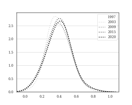
(a)

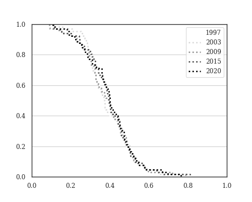
(b)

Figure 2: Weighted In-Degree Distribution

This figure visualizes the empirical distribution of weighted in and out-degrees across 66 non-government industries as defined in the Bureau of Economic Analysis (BEA) Make and Use Tables. The left panel shows the Gaussian kernel density estimate of the distribution, and the right panel shows the empirical counter-cumulative distribution function.

(a)

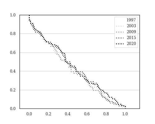
(b)

Figure 3: Weighted Out-Degree Distribution

This figure visualizes the empirical distribution of weighted in and out-degrees across 66 non-government industries as defined in the Bureau of Economic Analysis (BEA) Make and Use Tables. The left panel shows the Gaussian kernel density estimate of the distribution, and the right panel shows the empirical counter-cumulative distribution function.

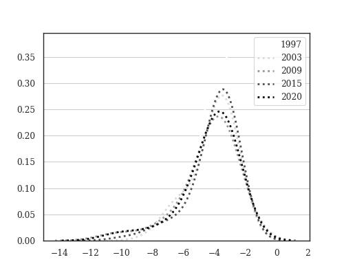
(a)

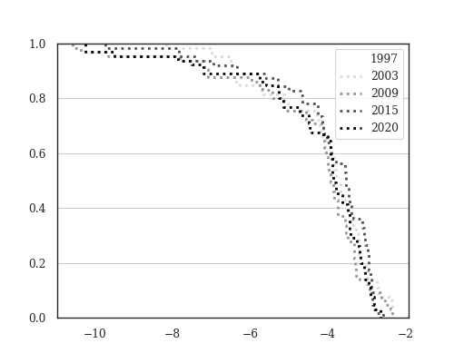
(b)

Figure 4: Distribution of Downstream Centrality

This figure visualizes the empirical distribution of weighted log eigenvector centrality of the upstream propagation matrix across 66 non-government industries as defined in the Bureau of Economic Analysis (BEA) Make and Use Tables. The left panel shows the Gaussian kernel density estimate of the distribution, and the right panel shows the empirical counter-cumulative distribution function.

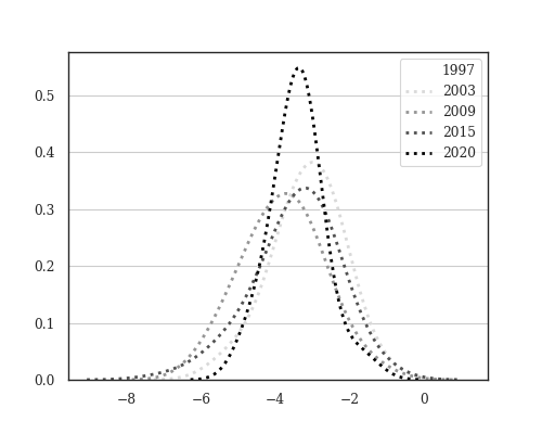
(a)

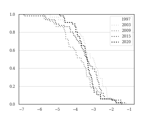
(b)

Figure 5: Distribution of Upstream Centrality

This figure visualizes the empirical distribution of weighted log eigenvector centrality of the upstream propagation matrix across 66 non-government industries as defined in the Bureau of Economic Analysis (BEA) Make and Use Tables. The left panel shows the Gaussian kernel density estimate of the distribution, and the right panel shows the empirical counter-cumulative distribution function.

Table 6: Correlation of Input-Output Shares

Entry	$\color[rgb]{0,0,0}w_{d,ij,t-1}$	$\color[rgb]{0,0,0}w_{u,ij,t-1}$	$\color[rgb]{0,0,0}h_{d,ij,t-1}$	$\color[rgb]{0,0,0}h_{u,ij,t-1}$	$\color[rgb]{0,0,0}w_{d,ij,t}$	$\color[rgb]{0,0,0}w_{u,ij,t}$	$\color[rgb]{0,0,0}h_{d,ij,t}$	$\color[rgb]{0,0,0}h_{u,ij,t}$
$\color[rgb]{0,0,0}w_{d,ij,t-1}$	1	0.086	0.970	0.096	0.991	0.086	0.961	0.096
$\color[rgb]{0,0,0}w_{u,ij,t-1}$		1	0.094	0.967	0.084	0.994	0.093	0.961
$\color[rgb]{0,0,0}h_{d,ij,t-1}$			1	0.110	0.962	0.095	0.990	0.111
$\color[rgb]{0,0,0}h_{u,ij,t-1}$				1	0.095	0.962	0.109	0.994
$\color[rgb]{0,0,0}w_{d,ij,t}$					1	0.086	0.970	0.096
$\color[rgb]{0,0,0}w_{u,ij,t}$						1	0.095	0.967
$\color[rgb]{0,0,0}h_{d,ij,t}$							1	0.111
$\color[rgb]{0,0,0}h_{u,ij,t}$								1

Note: This table report correlations between entries in the upstream and downstream propagation matrices $\color[rgb]{0,0,0}W_{qt}$ and their Leontief inverses $\color[rgb]{0,0,0}H_{qt}$. I construct annual matrices from the BEA Input-Output Accounts for 66 non-government industries between 1997-2020.

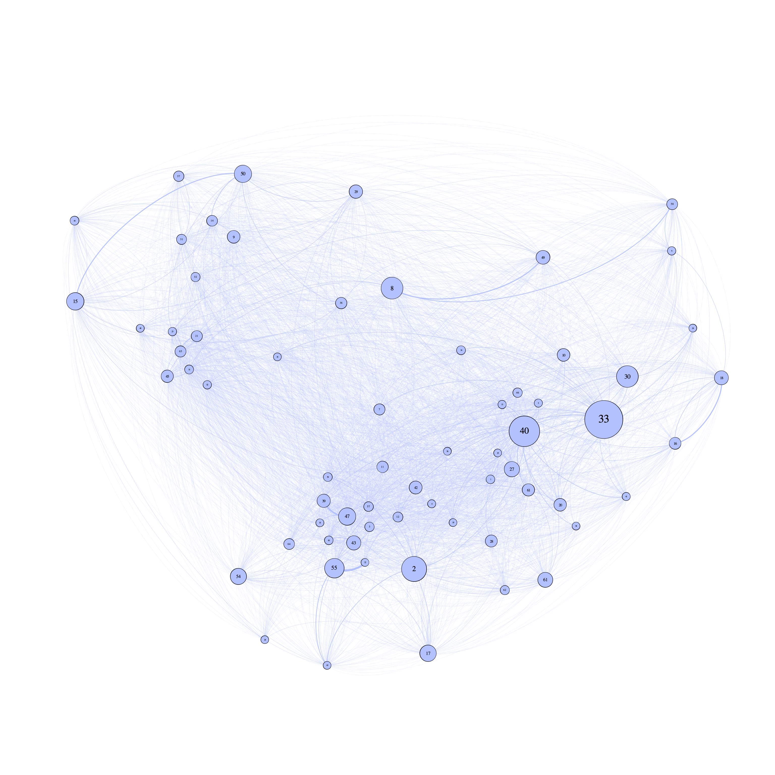
(a)

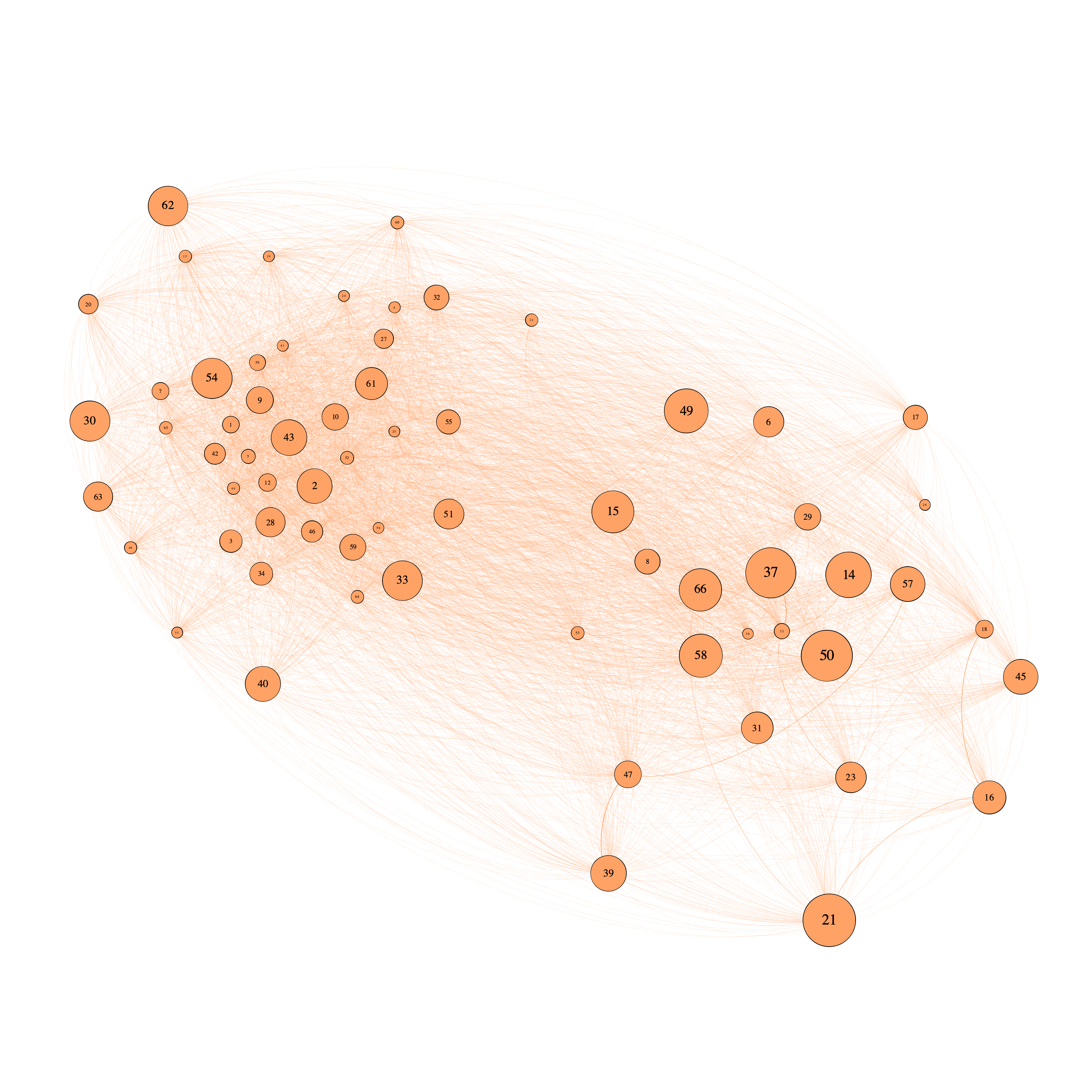
(b)

Figure 6: Visualizing Weighted Degree by Industry

The left panel shows the average weighted in-degree by sector as constructed from the downstream propagation network $\color[rgb]{0,0,0}\textbf{W}_{down}$. The right panel shows the average weighted in-degree by sector as constructed from the upstream propagation network $\color[rgb]{0,0,0}\textbf{W}_{up}$. The sectors are numbered identically in both panels, according to the BEA 66 non-government industry classification.

Appendix E Determinants of Network Variance

Table 7: Correlation in Predictors of Realized Variance

Predictor	$\color[rgb]{0,0,0}\beta_{vol}$	$\color[rgb]{0,0,0}C_{u}$	$\color[rgb]{0,0,0}C_{d}$	Between (d)	Between (s)	Size	Across (s)	Across (d)	VP	mkt ivol	mkt vol
$\color[rgb]{0,0,0}\beta_{vol}$	1	-0.329	-0.130	-0.308	0.072	0.285	0.061	-0.128	-0.225	0.287	0.406
$\color[rgb]{0,0,0}C_{u}$		1	0.284	0.356	-0.251	0.131	-0.441	0.319	0.423	-0.383	-0.396
$\color[rgb]{0,0,0}C_{d}$			1	0.588	-0.018	-0.128	-0.116	0.288	0.289	-0.003	-0.022
Between (d)				1	-0.205	-0.113	-0.156	0.704	0.708	-0.270	-0.311
Between (s)					1	-0.133	0.056	-0.163	-0.313	0.073	0.054
Size						1	-0.230	0.018	-0.111	-0.386	-0.275
Across (s)							1	-0.088	-0.159	0.205	0.255
Across (d)								1	0.627	-0.224	-0.249
VP									1	-0.279	-0.322
mkt ivol										1	0.965
mkt vol											1

Notes: This table reports the average correlation between predictors in the panel regression from Table 1. $\color[rgb]{0,0,0}C_{u}$ and $\color[rgb]{0,0,0}C_{d}$ refer to upstream and downstream centrality, the $\color[rgb]{0,0,0}(d)$ and $\color[rgb]{0,0,0}(s)$ labels denote demand and supply-side concentration, size is average output, and VP is vertical position. Idiosyncratic volatility is calculated from FF3 residual returns.

Table 8: Network Determinants of Industry Variance (TFP growth shocks)

Panel A: Market Return Variance
	(1)	(2)	(3)	(4)	(5)	(6)
Self-origin (demand)	0.365***	0.246***			0.217***	0.119***
	(0.038)	(0.039)			(0.021)	(0.022)
Across (demand)	0.100***	0.084***			0.085***	0.119***
	(0.020)	(0.018)			(0.020)	(0.019)
Between (demand)	0.043**	0.010			0.091***	-0.076***
	(0.018)	(0.022)			(0.019)	(0.020)
Self-origin (supply)			0.039*	0.149***	0.217***	0.119***
			(0.029)	(0.038)	(0.021)	(0.022)
Across (supply)			0.119***	0.147***	0.270***	0.170***
			(0.021)	(0.026)	(0.027)	(0.037)
Between (supply)			0.085***	0.042**	0.086***	0.179***
			(0.019)	(0.019)	(0.025)	(0.034)
Size		-0.202***		-0.325***		-0.183***
		(0.030)		(0.023)		(0.034)
Upstream centrality		-0.145**		0.129**		-0.238***
		(0.062)		(0.051)		(0.066)
Downstream centrality		1.956***		0.296**		2.137***
		(0.145)		(0.125)		(0.165)
Durability		1.088***		0.389***		1.164***
		(0.153)		(0.108)		(0.156)
Vertical position		3.890***		0.243***		4.063***
		(0.116)		(0.083)		(0.134)
Constant	-2.123	-0.634	-2.821	-0.096	-1.473	-0.693
Obs	2359	1626	2861	2138	2114	1471
Adj $\color[rgb]{0,0,0}R^{2}$	0.225	0.607	0.083	0.191	0.288	0.633
Panel B: Cash Flow Variance
	(1)	(2)	(3)	(4)	(5)	(6)
Self-origin (demand)	0.363***	0.009			0.190***	0.017
	(0.072)	(0.093)			(0.037)	(0.049)
Across (demand)	0.038	-0.050*			0.011	0.099**
	(0.039)	(0.039)			(0.040)	(0.042)
Between (demand)	0.136***	0.128***			0.156***	0.184***
	(0.037)	(0.042)			(0.039)	(0.047)
Self-origin (supply)			0.026	0.286***	0.190***	0.017
			(0.065)	(0.076)	(0.037)	(0.049)
Across (supply)			0.250***	0.384***	0.309***	0.107*
			(0.051)	(0.062)	(0.061)	(0.091)
Between (supply)			0.093**	0.169***	0.202***	0.162**
			(0.044)	(0.055)	(0.057)	(0.086)
Size		-0.161**		-0.333***		-0.155**
		(0.064)		(0.052)		(0.075)
Upstream centrality		-0.069		0.562***		-0.100
		(0.150)		(0.132)		(0.162)
Downstream centrality		2.193***		-0.070		2.315***
		(0.343)		(0.305)		(0.379)
Durability		2.204***		1.172***		2.307***
		(0.272)		(0.182)		(0.285)
Vertical position		3.502***		1.142*		3.590***
		(0.268)		(0.181)		(0.320)
Constant	-4.201	-0.711	-5.246	0.023	-4.123	-0.75
Obs	2359	1626	2861	2138	2114	1471
Adj $\color[rgb]{0,0,0}R^{2}$	0.074	0.248	0.017	0.08	0.087	0.271

Notes: This table reports panel regressions of realized industry variance on a variety of characteristics including the average log variance of supply and demand shocks, log concentration across trade partners, log concentration between trade partners, log total employment (size), log centrality of the upstream and downstream propagation networks, durability of output, vertical position in the supply chain, and industry cluster and year fixed effects. I calculate network components as the average value of 1000 bootstrap samples that randomly drop 10% of estimated pairwise non-zero correlations. In Panel A, the dependent variable is the log variance of annualized monthly returns on an equal-weighted industry portfolio. In Panel B, the dependent variable is the log variance of total quarterly year-on-year industry sales growth. I obtain return data from CRSP and sales data from Compustat. Concentration between and across trade partners are calculated as in 4 and 5, where I calculate the variance-covariance matrix of supply and demand shocks directly from four-factor TFP growth in the NBER-CES Database (Becker et al., 2016). Following Ahern (2013), I compute industry centrality as the eigenvector centrality of upstream and downstream propagation adjacency matrices. I obtain durability classifications from Gomes et al. (2009) and calculate vertical position of each industry as in Antràs et al. (2012) and Gofman et al. (2020). $\color[rgb]{0,0,0}^{***}$, $\color[rgb]{0,0,0}^{**}$ and $\color[rgb]{0,0,0}^{*}$ indicate significance at the 1%, 5%, and 10% levels, respectively. Standard error are clustered at the BEA 15 major industry group level. Sample is at an annual frequency from 1988 to 2017 for 479 BEA manufacturing industries.

Table 9: Network Determinants of Industry Variance (federal procurement shocks)

Panel A: Market Return Variance
	(1)	(2)	(3)	(4)	(5)	(6)
Self-origin (demand)	1.058***	0.903***			0.166*	0.558***
	(0.157)	(0.200)			(0.111)	(0.121)
Across (demand)	0.088**	0.314***			0.062*	0.356***
	(0.041)	(0.059)			(0.044)	(0.070)
Between (demand)	0.149***	0.153***			0.437***	0.261***
	(0.040)	(0.039)			(0.055)	(0.077)
Self-origin (supply)			0.219***	0.363***	0.166*	0.558***
			(0.044)	(0.056)	(0.111)	(0.121)
Across (supply)			0.142***	0.094*	0.072	0.088
			(0.036)	(0.052)	(0.072)	(0.079)
Between (supply)			0.150***	0.062	-0.063	-0.13
			(0.034)	(0.039)	(0.075)	(0.077)
Size		0.059		-0.242***		-0.033
		(0.053)		(0.047)		(0.053)
Upstream centrality		-2.434**		-4.885***		-2.140*
		(1.053)		(1.116)		(1.269)
Downstream centrality		10.76***		13.06***		10.55***
		(2.686)		(2.501)		(3.043)
Durability		4.128***		1.991***		3.884***
		(0.511)		(0.407)		(0.460)
Vertical position		11.74***		4.334***		10.66***
		(0.915)		(0.595)		(0.930)
Constant	-6.278	-3.489	-5.461	-4.234	-6.781	-3.419
Obs	839	666	1003	828	839	666
Adj R2	0.595	0.76	0.071	0.331	0.666	0.762
Panel B: Cash Flow Variance
	(1)	(2)	(3)	(4)	(5)	(6)
Self-origin (demand)	0.425	1.853*			0.267	1.025**
	(0.421)	(0.951)			(0.293)	(0.488)
Across (demand)	0.057	0.790***			0.183*	0.768***
	(0.090)	(0.215)			(0.121)	(0.207)
Between (demand)	0.309***	0.461***			0.524***	0.471**
	(0.091)	(0.121)			(0.146)	(0.199)
Self-origin (supply)			0.310***	0.004	0.267	1.025**
			(0.109)	(0.185)	(0.293)	(0.488)
Across (supply)			-0.184*	0.002	0.136	0.327*
			(0.101)	(0.139)	(0.193)	(0.258)
Between (supply)			0.235**	0.028	-0.247*	-0.268
			(0.092)	(0.112)	(0.192)	(0.244)
Size		0.183		-0.406***		-0.141
		(0.209)		(0.122)		(0.214)
Upstream centrality		1.430		3.297*		4.077*
		(3.309)		(2.975)		(3.421)
Downstream centrality		5.582		-5.585		0.810
		(8.923)		(6.799)		(8.718)
Durability		5.285***		1.175		5.536***
		(1.493)		(0.847)		(1.677)
Vertical position		12.20***		0.948		12.73***
		(3.184)		(1.236)		(4.096)
Constant	-1.223	-1.809	-7.991	1.81	-10.389	-0.263
Obs	839	666	1003	828	839	666
Adj R2	0.239	0.211	0.043	0.08	0.248	0.215

Notes: This table reports panel regressions of realized industry variance on a variety of characteristics including the average log variance of supply and demand shocks, log concentration across trade partners, log concentration between trade partners, log total employment (size), log centrality of the upstream and downstream propagation networks, durability of output, vertical position in the supply chain, and industry cluster and year fixed effects. I calculate network components as the average value of 1000 bootstrap samples that randomly drop 10% of estimated pairwise non-zero correlations In Panel A, the dependent variable is the log variance of annualized monthly returns on an equal-weighted industry portfolio. In Panel B, the dependent variable is the log variance of total quarterly year-on-year industry sales growth. I obtain return data from CRSP and sales data from Compustat. Concentration between and across trade partners are calculated as in 4 and 5, where I calculate the variance-covariance matrix of changes in total obligations from newly awarded federal procurement contracts measured from FPDS. Following Ahern (2013), I compute industry centrality as the eigenvector centrality of upstream and downstream propagation adjacency matrices. I obtain durability classifications from Gomes et al. (2009) and calculate vertical position of each industry as in Antràs et al. (2012) and Gofman et al. (2020). $\color[rgb]{0,0,0}^{***}$, $\color[rgb]{0,0,0}^{**}$ and $\color[rgb]{0,0,0}^{*}$ indicate significance at the 1%, 5%, and 10% levels, respectively. Standard error are clustered at the BEA 15 major industry level. Sample is at an annual frequency from 1991 to 2011 for 479 BEA manufacturing industries.

Table 10: Network Determinants of Industry Variance (technological proximity)

Panel A: Market Return Variance
	(1)	(2)	(3)	(4)	(5)	(6)
Self-origin (demand)	0.257***	0.352***			0.286***	0.308***
	(0.046)	(0.043)			(0.050)	(0.047)
Across (demand)	0.102***	0.120***			0.124***	0.145***
	(0.011)	(0.013)			(0.011)	(0.013)
Between (demand)	0.246***	0.117***			0.227***	0.058***
	(0.013)	(0.018)			(0.013)	(0.018)
Self-origin (supply)			0.290***	0.258***	0.229***	0.419***
			(0.035)	(0.039)	(0.040)	(0.043)
Across (supply)			0.009	0.032	0.223***	-0.035
			(0.027)	(0.036)	(0.031)	(0.042)
Between (supply)			0.190***	0.168***	0.284***	0.143**
			(0.031)	(0.043)	(0.034)	(0.051)
Size		-0.343***		-0.312***		-0.334***
		(0.031)		(0.027)		(0.030)
Upstream centrality		-0.755***		-0.102*		-0.543***
		(0.108)		(0.087)		(0.104)
Downstream centrality		3.933***		1.052***		3.632***
		(0.279)		(0.190)		(0.275)
Durability		-0.195*		-0.177*		-0.076
		(0.112)		(0.098)		(0.108)
Vertical position		1.669***		0.130		2.160***
		(0.152)		(0.086)		(0.172)
Constant	-7.926	-1.275	-3.85	-0.341	-8.468	-1.177
Obs	1994	1467	1994	1467	1994	1467
Adj R2	0.593	0.642	0.127	0.279	0.61	0.665
Panel B: Cash Flow Variance
	(1)	(2)	(3)	(4)	(5)	(6)
Self-origin (demand)	0.391***	0.521***			0.473***	0.548***
	(0.103)	(0.103)			(0.102)	(0.103)
Across (demand)	0.065**	0.061*			0.050*	0.049*
	(0.028)	(0.033)			(0.029)	(0.034)
Between (demand)	0.253***	0.139***			0.172**	0.217*
	(0.030)	(0.045)			(0.077)	(0.122)
Self-origin (supply)			-0.019	-0.245***	-0.162**	-0.185*
			(0.076)	(0.087)	(0.079)	(0.097)
Across (supply)			0.175***	0.138*	0.072	0.160*
			(0.067)	(0.100)	(0.068)	(0.102)
Between (supply)			0.307***	0.228**	0.271***	0.179***
			(0.076)	(0.119)	(0.031)	(0.048)
Size		-0.298***		-0.332***		-0.298***
		(0.070)		(0.066)		(0.071)
Upstream centrality		0.113		0.355*		-0.068
		(0.267)		(0.276)		(0.280)
Downstream centrality		3.217***		0.311		3.555***
		(0.665)		(0.599)		(0.680)
Durability		0.574***		0.265*		0.481**
		(0.210)		(0.211)		(0.218)
Vertical position		1.922***		-0.311		1.493***
		(0.323)		(0.208)		(0.373)
Constant	-10.991	-1.043	-5.631	-0.101	-11.776	-1.152
Obs	1994	1467	1994	1467	1994	1467
Adj R2	0.21	0.23	0.011	0.051	0.216	0.233

Notes: This table reports panel regressions of realized industry variance on a variety of characteristics including the average log variance of supply and demand shocks, log concentration across trade partners, log concentration between trade partners, log total employment (size), log centrality of the upstream and downstream propagation networks, durability of output, vertical position in the supply chain, and industry cluster and year fixed effects. I calculate network components as the average value of 1000 bootstrap samples that randomly drop 10% of estimated pairwise non-zero correlations. In Panel A, the dependent variable is the log variance of annualized monthly returns on an equal-weighted industry portfolio. In Panel B, the dependent variable is the log variance of total quarterly year-on-year industry sales growth. I obtain return data from CRSP and sales data from Compustat. Concentration between and across trade partners are calculated as in 4 and 5, where I calculate the variance-covariance matrix of supply and demand shocks using the weighted technological similarity scores following Bloom and Shankerman (2013). Following Ahern (2013), I compute industry centrality as the eigenvector centrality of upstream and downstream propagation adjacency matrices. I obtain durability classifications from Gomes et al. (2009) and calculate vertical position of each industry as in Antràs et al. (2012) and Gofman et al. (2020). $\color[rgb]{0,0,0}^{***}$, $\color[rgb]{0,0,0}^{**}$ and $\color[rgb]{0,0,0}^{*}$ indicate significance at the 1%, 5%, and 10% levels, respectively. Standard errors are clustered at the BEA 15 major industry group level. Sample is at an annual frequency from 1988 to 2018 for 479 BEA manufacturing industries.

Table 11: Network Determinants of Industry Variance (product similarity)

Panel A: Market Return Variance
	(1)	(2)	(3)	(4)	(5)	(6)
Self-origin (demand)	0.136**	0.354***			0.303***	0.321***
	(0.056)	(0.040)			(0.046)	(0.041)
Across (demand)	0.103***	0.071***			-0.065***	0.051***
	(0.013)	(0.011)			(0.013)	(0.012)
Between (demand)	0.131***	0.081**			0.384***	0.058***
	(0.013)	(0.012)			(0.014)	(0.016)
Self-origin (supply)			0.096***	0.056*	-0.047	0.207***
			(0.027)	(0.033)	(0.033)	(0.034)
Across (supply)			0.147***	0.137***	0.186***	-0.000
			(0.015)	(0.020)	(0.020)	(0.021)
Between (supply)			-0.086***	-0.106***	-0.362***	-0.071***
			(0.012)	(0.016)	(0.017)	(0.020)
Size		-0.361***		-0.257***		-0.310***
		(0.025)		(0.021)		(0.024)
Upstream centrality		-0.149***		0.031		-0.176***
		(0.053)		(0.049)		(0.055)
Downstream centrality		2.660***		0.811***		2.891***
		(0.174)		(0.117)		(0.180)
Durability		0.216**		0.265***		0.286***
		(0.102)		(0.096)		(0.098)
Vertical position		3.414***		0.368***		3.336***
		(0.086)		(0.076)		(0.106)
Constant	-5.915	-0.862	-3.631	-0.263	-8.380	-0.937
Obs	3800	2430	3819	2430	3800	2430
Adj $\color[rgb]{0,0,0}R^{2}$	0.359	0.625	0.037	0.175	0.488	0.639
Panel B: Cash Flow Variance
	(1)	(2)	(3)	(4)	(5)	(6)
Self-origin (demand)	0.357***	0.549***			0.544***	0.558***
	(0.091)	(0.090)			(0.091)	(0.091)
Across (demand)	0.112***	0.055**			-0.059**	0.011
	(0.023)	(0.027)			(0.025)	(0.030)
Between (demand)	0.118***	0.066**			0.373***	0.108***
	(0.023)	(0.030)			(0.027)	(0.040)
Self-origin (supply)			0.030	-0.026	-0.141*	0.084*
			(0.060)	(0.073)	(0.062)	(0.078)
Across (supply)			0.129***	0.199***	0.170***	0.091**
			(0.029)	(0.039)	(0.031)	(0.043)
Between (supply)			-0.074***	-0.156***	-0.347***	-0.157***
			(0.023)	(0.032)	(0.028)	(0.041)
Size		-0.313***		-0.242***		-0.273***
		(0.050)		(0.048)		(0.051)
Upstream centrality		0.185*		0.327**		0.090
		(0.135)		(0.132)		(0.138)
Downstream centrality		3.213***		0.791***		3.587***
		(0.406)		(0.300)		(0.413)
Durability		1.097***		1.104***		1.145***
		(0.171)		(0.171)		(0.170)
Vertical position		3.495***		0.226		3.102***
		(0.193)		(0.164)		(0.251)
Constant	-10.060	-1.041	-5.694	-0.256	-12.580	-1.162
Obs	3800	2430	3819	2430	3800	2430
Adj $\color[rgb]{0,0,0}R^{2}$	0.15	0.235	0.005	0.047	0.205	0.242

Notes: This table reports panel regressions of realized industry variance on a variety of characteristics including the average log variance of supply and demand shocks, log concentration across trade partners, log concentration between trade partners, log total employment (size), log centrality of the upstream and downstream propagation networks, durability of output, vertical position in the supply chain, and industry cluster and year fixed effects. I calculate network components as the average value of 1000 bootstrap samples that randomly drop 10% of estimated pairwise non-zero correlations. In Panel A, the dependent variable is the log variance of annualized monthly returns on an equal-weighted industry portfolio. In Panel B, the dependent variable is the log variance of total quarterly year-on-year industry sales growth. I obtain return data from CRSP and sales data from Compustat. Concentration between and across trade partners are calculated as in 4 and 5, where I calculate the variance-covariance matrix of supply and demand shocks using the product similarity distances from Hoberg and Phillips (2016). Following Ahern (2013), I compute industry centrality as the eigenvector centrality of upstream and downstream propagation adjacency matrices. I obtain durability classifications from Gomes et al. (2009) and calculate vertical position of each industry as in Antràs et al. (2012) and Gofman et al. (2020). $\color[rgb]{0,0,0}^{***}$, $\color[rgb]{0,0,0}^{**}$ and $\color[rgb]{0,0,0}^{*}$ indicate significance at the 1%, 5%, and 10% levels, respectively. Standard error are clustered at the BEA 15 major industry group level. Sample is at an annual frequency from 1988 to 2018 for 479 BEA manufacturing industries.

Appendix F Simulation Evidence

Proposition 2.3 claims that there is no matrix $\color[rgb]{0,0,0}\mathbf{W}$ with entries $\color[rgb]{0,0,0}w_{ij}\in(0,1)$ such that Assumption 2.2 and (1) are satisfied. This implies that $\color[rgb]{0,0,0}\Delta:=||(\mathbf{I}-\mathbf{W})\mathbf{\Sigma}_{y}(\mathbf{I}-\mathbf{W})-\mathbf{\Sigma}_{u}||$ should always be different from zero when $\color[rgb]{0,0,0}\mathbf{\Sigma}_{u}$ is diagonal. I test $\color[rgb]{0,0,0}H_{0}:\Delta=0$ numerically as follows:

1. Fix dimension $\color[rgb]{0,0,0}n$, number of iterations $\color[rgb]{0,0,0}S$, and consider the following constrained optimization problem:

   $$\color[rgb]{0,0,0}\displaystyle f_{min}(\mathbf{\Sigma}_{u}) \color[rgb]{0,0,0}\displaystyle=\min_{w_{ij,i\neq j}\in(0,1)}f(\mathbf{W};\mathbf{\Sigma}_{u})=\min_{w_{ij,i\neq j}\in(0,1)}\bigg{|}\bigg{|}\mathbf{\Sigma}_{u}-(\mathbf{I}_{n}-\mathbf{W})^{-1}\mathbf{\Sigma}_{u}(\mathbf{I}_{n}-\mathbf{W}^{\top})^{-1}\bigg{|}\bigg{|}_{F},$$ (49)

2. Draw two random samples $\color[rgb]{0,0,0}S_{u}^{d}$ and $\color[rgb]{0,0,0}S_{u}^{*}$ for the variance-covariance matrix of residuals $\color[rgb]{0,0,0}\mathbf{\Sigma}_{u}$ such that $\color[rgb]{0,0,0}S_{u}^{d}$ is diagonal and $\color[rgb]{0,0,0}S_{u}^{*}$ is not. I sample the non-diagonal matrix as follows:

   $$\color[rgb]{0,0,0}\displaystyle S_{u}^{*}(s) \color[rgb]{0,0,0}\displaystyle\sim_{iid}\mathcal{W}^{-1}(\mathbf{\Psi}_{u},\nu),$$

   where $\color[rgb]{0,0,0}\mathcal{W}^{-1}(\mathbf{\Psi},\nu)$ denotes an Inverse-Wishart random variable with scale $\color[rgb]{0,0,0}\mathbf{\Psi}$ and degrees of freedom $\color[rgb]{0,0,0}\nu>n-1$. On the other hand, the diagonal matrix is given by:

   $$\color[rgb]{0,0,0}\displaystyle S_{u}^{d}(s)=\text{diag}(X_{1},...,X_{n}),\quad X_{i}\sim_{iid}\Gamma^{-1}(\alpha_{i},\beta_{i}),$$

   where $\color[rgb]{0,0,0}\Gamma^{-1}(\alpha_{i},\beta_{i})$ denotes an Inverse-Gamma distribution such that $\color[rgb]{0,0,0}\alpha_{i}>1$ and $\color[rgb]{0,0,0}\mathbb{E}[X_{i}]=\frac{\beta_{i}}{\alpha_{i}-1}=[\Psi_{u}]_{i}i$ for all $\color[rgb]{0,0,0}i$. This ensures that the means of diagonal elements are the same across the two samples.

3. Solve equation (49) using off-the-shelf constrained quasi-Newton algorithms in both cases and construct $\color[rgb]{0,0,0}S$ realizations of $\color[rgb]{0,0,0}f_{s}^{*}=f_{min}(S_{u}^{*})$ and $\color[rgb]{0,0,0}f_{s}^{d}=f_{min}(S_{u}^{d})$ for $\color[rgb]{0,0,0}s=1,...,S$.

4. Construct the numerical p-value using

   $$\color[rgb]{0,0,0}p=\frac{1}{S}\sum_{s=1}^{S}\mathbbm{1}\{f_{s}^{*}\geq f_{s}^{d}\},$$

   and repeat Step 3 for different values of $\color[rgb]{0,0,0}n$ and $\color[rgb]{0,0,0}\mathbf{\Phi}_{u}$. Reported results in Table 12.

5. For optimal $\color[rgb]{0,0,0}W_{min}^{spec}=\operatorname*{arg\,min}f(W,S_{u}^{spec})$, consider the $\color[rgb]{0,0,0}n\times n$ elementwise difference $\color[rgb]{0,0,0}\tilde{\Delta}_{s}$ for each iteration $\color[rgb]{0,0,0}s$:

   $$\color[rgb]{0,0,0}\displaystyle\tilde{\Delta}_{s}=f(W_{min}^{d},S_{u}^{d})-f({W}_{min}^{*},S_{u}^{*})$$

   Then I test the marginal hypotheses $\color[rgb]{0,0,0}H_{0}:[\tilde{\Delta}_{s}]_{ij}=0$ for all $\color[rgb]{0,0,0}i,j$. This test corresponds to the numerical t-statistic $\color[rgb]{0,0,0}t_{ij}=m_{ij}/SE_{ij}$, where $\color[rgb]{0,0,0}m_{ij}$ and $\color[rgb]{0,0,0}SE_{ij}$ are the mean and standard error of $\color[rgb]{0,0,0}[\tilde{\Delta}_{s}]_{ij}$, respectively. Reported results in Table 13.

Table 12: Simulation p-values

Specification	n=2	n=3	n=4	n=5
(1)	0.000	0.002	0.036	0.004
(2)	0.000	0.000	0.041	0.005
(3)	0.000	0.003	0.046	0.006
(4)	0.000	0.001	0.048	0.009
(5)	0.000	0.000	0.053	0.008
(6)	0.000	0.003	0.060	0.008
(7)	0.000	0.001	0.061	0.006
(8)	0.000	0.001	0.061	0.010
(9)	0.000	0.004	0.068	0.011
(10)	0.000	0.001	0.072	0.011

Note: this table reports numerical p-values from the procedure described in Appendix F for different values of $\color[rgb]{0,0,0}n$ and $\color[rgb]{0,0,0}\mathbf{\Phi}$. Number of iterations is $\color[rgb]{0,0,0}S=1000$.

Table 13: Simulation t-statistics

n=2	n=3	n=4	n=5
121	-27	-54	-118
863	48	133	201
861	60	163	152
-504	48	2	-502
	-68	133	-152
	80	-247	201
	60	-26	-583
	80	190	172
	-91	163	205
		-26	61
		-255	152
		204	172
		2	-177
		190	174
		204	138
		-60	-502
			205
			174
			-89
			-334
			-152
			61
			138
			-334
			-75

Note: this table reports elementwise t-statistcs from the procedure described in Appendix F for different values of $\color[rgb]{0,0,0}n$ and a fixed value $\color[rgb]{0,0,0}\mathbf{\Phi}$. Number of iterations is $\color[rgb]{0,0,0}S=1000$.

Appendix G Comovement in Industry Volatility

Recent research documents significant common variation in both market and fundamental volatility at the granular level. Importantly, the factor structure in volatility is significant even after removing all common variation in returns and cash flow growth, which suggests that this is being driven by underlying sources of systematic risk and rather than an omitted set of returns or sales growth factors. When economic units are connected via input-output networks, a shock to any given unit can generate systematic effects. Moreover, networks mechanically generate volatility comovement regardless of whether shocks to individual units are uncorrelated. When shocks are correlated, this comovement is even more pronounced.

My results so far establish a significant relationship between network concentration across and between customers and suppliers and realized variance. Consequently, comovement in supply chain concentration should also generate comovement in realized variance. Table 14 reports average loadings and $\color[rgb]{0,0,0}R^{2}$ values of univariate factor regressions for panel of industry network concentration and realized volatility measures. The main takeaway is that 20-30% of dynamic variation in input-output concentration and return and sales growth volatilities across industries of these variables can be explained by a single factor. Moreover, there is a significant degree of comovement between these common factors. That is, network concentration factors can explain up to 40% of time-series variation in both market and sales growth volatility factors. These results are robust to a variety of specifications.

Table 14: Comovement in Industry Variance

Panel A: Loadings
Factor / Outcome	Across (d)	Between (d)	Across (s)	Between (s)	Var (mkt)	Var (cf)
Across (d)	0.788	1.576	0.364	0.507	0.410	0.574
Between (d)	0.584	0.735	0.394	0.567	0.206	0.383
Across (s)	0.701	1.185	0.700	0.518	0.156	0.497
Between (s)	0.455	0.422	0.401	0.736	0.157	0.310
Var (mkt)	0.091	0.124	0.016	0.035	0.880	0.185
Var (cf)	0.109	0.181	0.156	0.218	0.283	0.721
Panel B: $\color[rgb]{0,0,0}R^{2}$ (avg univariate)
Factor / Outcome	Across (d)	Between (d)	Across (s)	Between (s)	Var (mkt)	Var (cf)
Across (d)	0.201	0.258	0.217	0.318	0.170	0.079
Between (d)	0.189	0.318	0.257	0.400	0.174	0.087
Across (s)	0.164	0.274	0.229	0.344	0.168	0.082
Between (s)	0.189	0.322	0.265	0.347	0.165	0.086
Var (mkt)	0.042	0.046	0.041	0.042	0.343	0.068
Var (cf)	0.063	0.097	0.085	0.115	0.147	0.104
Panel C: $\color[rgb]{0,0,0}R^{2}$ (aggregate)
Factor / Outcome	Across (d)	Between (d)	Across (s)	Between (s)	Var (mkt)	Var (cf)
Across (d)	1	0.620	0.575	0.566	0.373	0.352
Between (d)		1	0.628	0.670	0.255	0.422
Across (s)			1	0.668	0.196	0.469
Between (s)				1	0.229	0.428
Var (mkt)					1	0.165
Var (cf)						1

Notes: This table reports the results of factor regressions for industry variance components. I calculate factors as the first principal component of an industry panel of the variable of interest. Panels A and B report the average loading and $\color[rgb]{0,0,0}R^{2}$ from the regressions $\color[rgb]{0,0,0}outcome_{it}=\alpha_{i}+\beta_{i}\cdot f_{t}+u_{it}$, respectively. Each column, row pair denotes a different outcome, factor pair. Panel C reports the $\color[rgb]{0,0,0}R^{2}$ of aggregate time-series regressions of factor pairs (i.e., $\color[rgb]{0,0,0}y_{t}=\alpha+\beta\cdot x_{t}+u_{t}$, where $\color[rgb]{0,0,0}y_{t}$ is the column factor and $\color[rgb]{0,0,0}x_{t}$ is the row factor). All variables are log-transformed. Sample is at an annual frequency from 1997 to 2019 for 66 non-government BEA industries.

Appendix H Additional Firm-Level Results

Table 15: Predicting Firm Sales Growth

Variable	(1)	(2)	(3)
$\color[rgb]{0,0,0}a_{t-1}$	0.031**	0.029**	0.007**
	(0.002)	(0.001)	(0.000)
$\color[rgb]{0,0,0}g_{t-1}$	-0.016**	-0.018**	0.015
	(0.003)	(0.003)	(0.011)
$\color[rgb]{0,0,0}ROA_{i,t-1}$	0.080**	0.063**	0.064**
	(0.003)	(0.002)	(0.002)
$\color[rgb]{0,0,0}size_{i,t-1}$	-0.008**	-0.008**	-0.008**
	(0.000)	(0.000)	(0.000)
$\color[rgb]{0,0,0}age_{i}$	0.037**	0.050**	0.046**
	(0.004)	(0.004)	(0.003)
Constant	0.44	0.372	0.39
Obs	259,976	259,976	259,976
Adj R2	0.265	0.259	0.258

Notes: This table reports the regression results based on the model in (21). The dependent variable is year-on-year quarterly sales growth and the covariates are aggregate TFP growth from Fernald (2012), procurement proxy from Briganti and Sellemi (2022), log return on assets, size (log market value), and age as year appears on the database. Each column reports results for different industry aggregations: (1) is 66 BEA non-government industries, (2) is 405 BEA non-government industries, and (3) is 15 major BEA non-government industries. Standard errors are clustered at the same granularity. $\color[rgb]{0,0,0}**$ and $\color[rgb]{0,0,0}*$ indicates significance at the 1% and 5% levels, resp. Sample is quarterly between 1997-2019 for 10,700 firms.

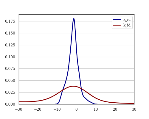
(a)

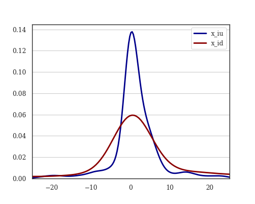
(b)

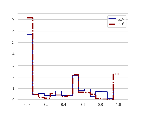
(c)

Figure 7: Distribution of Calibrated Propensities with No Network Connections

Notes: This figure plots the kernel density of calibrated parameters $\color[rgb]{0,0,0}k_{iq}$ and $\color[rgb]{0,0,0}x_{iq}$ as described in Section 5. Note that $\color[rgb]{0,0,0}\bar{p}_{iq}=1/(1+\exp(-k_{iq}x_{iq}))$.

(a)

(b)

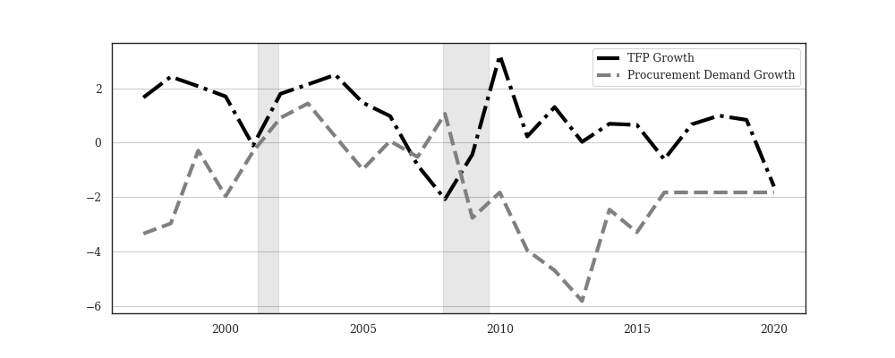
(c)

Figure 8: Network Propagation Risk Factors

Notes: This figure plots the time series of network propagation risk factors (Panel A), the cross-sectional average industry substitutability (Panel B), and aggregate TFP and procurement demand growth (Panel C). Shaded regions indicate NBER-dated recession periods.

Table 16: Descriptive Statistics Calibrated Firm Parameters

Table 17: One-Way Sorted Portfolios on Network Propagation Factors (controlling for volatility factors)

Panel A: One-way sorts on upstream propagation beta (controlling for $\color[rgb]{0,0,0}a_{t}$, $\color[rgb]{0,0,0}g_{t}$, and $\color[rgb]{0,0,0}\sigma_{t}^{civ}$)
	1 (Low)	2	3	4	5 (High)	H-L	t(H-L)	MR p-val
$\color[rgb]{0,0,0}\mathbb{E}[r]-r_{f}$	12.97	12.12	11.34	10.44	10.11	-2.86	-5.83	0.22
$\color[rgb]{0,0,0}\alpha_{capm}$	-0.04	-0.21	-0.21	-0.28	-0.68	-0.64	-4.06	0.00
$\color[rgb]{0,0,0}\alpha_{ff3}$	-0.10	-0.14	-0.17	-0.25	-0.39	-0.29	-0.83	0.01
Volatility (%)	13.37	14.81	14.71	19.1	12.64	-	-	-
Book-to-market	0.52	0.53	0.58	0.54	0.50	-	-	-
Market value ($bn)	12.18	6.21	18.07	6.14	15.75	-	-	-
Panel B: One-way sorts on downstream propagation beta (controlling for $\color[rgb]{0,0,0}a_{t}$, $\color[rgb]{0,0,0}g_{t}$, and $\color[rgb]{0,0,0}\sigma_{t}^{civ}$)
	1 (Low)	2	3	4	5 (High)	H-L	t(H-L)	MR p-val
$\color[rgb]{0,0,0}\mathbb{E}[r]-r_{f}$	14.97	12.94	12.15	9.78	9.35	-5.61	-9.36	0.09
$\color[rgb]{0,0,0}\alpha_{capm}$	0.03	-0.24	-0.29	-0.32	-0.39	-0.43	-1.88	0.00
$\color[rgb]{0,0,0}\alpha_{ff3}$	-0.02	-0.10	-0.26	-0.29	-0.30	-0.29	-3.40	0.01
Volatility (%)	18.69	16.42	12.11	14.20	13.02	-	-	-
Book-to-market	0.59	0.55	0.51	0.51	0.52	-	-	-
Market value ($bn)	5.11	12.13	8.96	16.43	15.64	-	-	-
Panel C: One-way sorts on upstream propagation beta (controlling for $\color[rgb]{0,0,0}a_{t}$, $\color[rgb]{0,0,0}g_{t}$, and $\color[rgb]{0,0,0}\sigma_{t}^{mkt}$)
	1 (Low)	2	3	4	5 (High)	H-L	t(H-L)	MR p-val
$\color[rgb]{0,0,0}\mathbb{E}[r]-r_{f}$	13.83	13.07	11.33	10.10	9.73	-4.09	-8.10	0.21
$\color[rgb]{0,0,0}\alpha_{capm}$	0.01	-0.26	-0.28	-0.35	-0.45	-0.47	-6.84	0.04
$\color[rgb]{0,0,0}\alpha_{ff3}$	-0.07	-0.17	-0.20	-0.29	-0.30	-0.23	-2.06	0.03
Volatility (%)	13.68	16.44	17.09	14.12	13.03	-	-	-
Book-to-market	0.51	0.54	0.55	0.54	0.53	-	-	-
Market value ($bn)	11.43	5.87	7.24	19.44	14.40	-	-	-
Panel D: One-way sorts on downstream propagation beta (controlling for $\color[rgb]{0,0,0}a_{t}$, $\color[rgb]{0,0,0}g_{t}$, and $\color[rgb]{0,0,0}\sigma_{t}^{mkt}$)
	1 (Low)	2	3	4	5 (High)	H-L	t(H-L)	MR p-val
$\color[rgb]{0,0,0}\mathbb{E}[r]-r_{f}$	13.66	13.5	12.67	9.77	9.24	-4.42	-7.17	0.37
$\color[rgb]{0,0,0}\alpha_{capm}$	0.07	-0.26	-0.32	-0.39	-0.41	-0.48	-1.81	0.00
$\color[rgb]{0,0,0}\alpha_{capm}$	0.02	-0.17	-0.24	-0.25	-0.33	-0.35	-1.52	0.01
Volatility (%)	19.47	12.94	15.7	14.27	13.03	-	-	-
Book-to-market	0.63	0.54	0.44	0.53	0.52	-	-	-
Market value ($bn)	4.60	10.24	13.33	15.77	14.30	-	-	-

Notes: This table reports average excess returns and post-sample alphas in annual percentages for value-weighted portfolios sorted into quintiles on annual upstream and downstream propagation factors. Sample is between 1997-2021 for more than 10,000 stocks belonging to the BEA 66 non-government industry classifications. Panels A and B control for productivity growth and federal procurement demand growth, while Panels C and D have no controls. I also report average return volatility, book-to-market ratio and market value for each portfolio. To test for significant return spreads, I report $\color[rgb]{0,0,0}t$-statistics for the null hypothesis $\color[rgb]{0,0,0}H_{0}:xr_{5}=xr_{1}$, where $\color[rgb]{0,0,0}xr_{q}$ is the average return of the $\color[rgb]{0,0,0}q^{th}$ quintile single sorted portfolio. Moreover, I report p-values for the test $\color[rgb]{0,0,0}H_{0}:xr_{q+1}<xr_{q}\forall q\leq 4$, calculated via bootstrap following Patton and Timmermann (2010).

References

- Acemoglu et al. (2012) D. Acemoglu, V. M. Carvalho, A. Ozdaglar, and A. Tahbaz-Salehi. The network origins of aggregate fluctuations. Econometrica, 80(5):1977–2016, 2012. doi: https://doi.org/10.3982/ECTA9623. URL https://onlinelibrary.wiley.com/doi/abs/10.3982/ECTA9623.
- Acemoglu et al. (2016) D. Acemoglu, U. Akcigit, and W. Kerr. Networks and the macroeconomy: An empirical exploration. NBER Macroeconomics Annual, 30(1):273–335, 2016. URL https://EconPapers.repec.org/RePEc:ucp:macann:doi:10.1086/685961.
- Ahern (2013) K. R. Ahern. Network centrality and the cross section of stock returns. Economics of Networks eJournal, 2013.
- Ang et al. (2006) A. Ang, R. J. Hodrick, Y. Xing, and X. Zhang. The cross-section of volatility and expected returns. The Journal of Finance, 61(1):259–299, 2006. doi: https://doi.org/10.1111/j.1540-6261.2006.00836.x. URL https://onlinelibrary.wiley.com/doi/abs/10.1111/j.1540-6261.2006.00836.x.
- Antràs et al. (2012) P. Antràs, D. Chor, T. Fally, and R. Hillberry. Measuring the upstreamness of production and trade flows. American Economic Review, 102(3):412–416, May 2012. doi: 10.1257/aer.102.3.412. URL https://doi.org/10.1257/aer.102.3.412.
- Autor et al. (2013) D. H. Autor, D. Dorn, and G. H. Hanson. The china syndrome: Local labor market effects of import competition in the united states. American Economic Review, 103(6):2121–68, October 2013. doi: 10.1257/aer.103.6.2121. URL https://www.aeaweb.org/articles?id=10.1257/aer.103.6.2121.
- Baqaee and Farhi (2019) D. R. Baqaee and E. Farhi. The macroeconomic impact of microeconomic shocks: Beyond hulten’s theorem. Econometrica, 87(4):1155–1203, 2019. doi: https://doi.org/10.3982/ECTA15202. URL https://onlinelibrary.wiley.com/doi/abs/10.3982/ECTA15202.
- Barrot and Sauvagnat (2016) J.-N. Barrot and J. Sauvagnat. Input Specificity and the Propagation of Idiosyncratic Shocks in Production Networks *. The Quarterly Journal of Economics, 131(3):1543–1592, 05 2016. ISSN 0033-5533. doi: 10.1093/qje/qjw018. URL https://doi.org/10.1093/qje/qjw018.
- Becker et al. (2016) A. Becker, W. Gray, and J. Marvakov. Nber-ces manufacturing industry database: Technical notes. National Bureau of Economic Research, 2016. URL https://www.nber.org/research/data/nber-ces-manufacturing-industry-database.
- Bloom and Shankerman (2013) N. Bloom and M. Shankerman. Identifying technology spillovers and product market rivalry. Econometrica, 81(4):1347–1393, 2013. doi: 10.3982/ecta9466. URL https://doi.org/10.3982/ecta9466.
- Breza et al. (2020) E. Breza, A. G. Chandrasekhar, T. H. McCormick, and M. Pan. Using aggregated relational data to feasibly identify network structure without network data. American Economic Review, 110(8):2454–84, August 2020. doi: 10.1257/aer.20170861. URL https://www.aeaweb.org/articles?id=10.1257/aer.20170861.
- Briganti and Sellemi (2022) E. Briganti and V. Sellemi. Who anticipates government spending? evidence from defense procurement. Working Paper, 2022.
- Engle (2002) R. Engle. Dynamic conditional correlation: A simple class of multivariate generalized autoregressive conditional heteroskedasticity models. Journal of Business & Economic Statistics, 20(3):339–350, 2002. ISSN 07350015. URL http://www.jstor.org/stable/1392121.
- Fernald (2012) J. G. Fernald. A quarterly, utilization-adjusted series on total factor productivity. Working Paper Series 2012-19, Federal Reserve Bank of San Francisco, 2012. URL https://ideas.repec.org/p/fip/fedfwp/2012-19.html.
- Fioruci et al. (2013) J. A. Fioruci, R. S. Ehlers, and M. G. A. Filho. Bayesian multivariate GARCH models with dynamic correlations and asymmetric error distributions. Journal of Applied Statistics, 41(2):320–331, Oct. 2013. doi: 10.1080/02664763.2013.839635. URL https://doi.org/10.1080/02664763.2013.839635.
- Gabaix (2011) X. Gabaix. The granular origins of aggregate fluctuations. Econometrica, 79:733–772, 2011.
- Gofman et al. (2020) M. Gofman, G. Segal, and Y. Wu. Production Networks and Stock Returns: The Role of Vertical Creative Destruction. The Review of Financial Studies, 33(12):5856–5905, 03 2020. ISSN 0893-9454. doi: 10.1093/rfs/hhaa034. URL https://doi.org/10.1093/rfs/hhaa034.
- Gomes et al. (2009) J. F. Gomes, L. Kogan, and M. Yogo. Durability of output and expected stock returns. Journal of Political Economy, 117(5):941–986, Oct. 2009. doi: 10.1086/648882. URL https://doi.org/10.1086/648882.
- Herskovic (2018a) B. Herskovic. Networks in production: Asset pricing implications. The Journal of Finance, 73(4):1785–1818, 2018a. doi: https://doi.org/10.1111/jofi.12684. URL https://onlinelibrary.wiley.com/doi/abs/10.1111/jofi.12684.
- Herskovic (2018b) B. Herskovic. Networks in Production: Asset Pricing Implications: Networks in Production: Asset Pricing Implications. The Journal of Finance, 73(4):1785–1818, Aug. 2018b. ISSN 00221082. doi: 10.1111/jofi.12684. URL http://doi.wiley.com/10.1111/jofi.12684.
- Herskovic et al. (2016) B. Herskovic, B. Kelly, H. Lustig, and S. Van Nieuwerburgh. The common factor in idiosyncratic volatility: Quantitative asset pricing implications. Journal of Financial Economics, 119(2):249–283, 2016. ISSN 0304-405X. doi: https://doi.org/10.1016/j.jfineco.2015.09.010. URL https://www.sciencedirect.com/science/article/pii/S0304405X15001774.
- Herskovic et al. (2020a) B. Herskovic, B. Kelly, H. Lustig, and S. Van Nieuwerburgh. Firm volatility in granular networks. Journal of Political Economy, 0(0):000–000, 2020a. doi: 10.1086/710345. URL https://doi.org/10.1086/710345.
- Herskovic et al. (2020b) B. Herskovic, B. Kelly, H. Lustig, and S. Van Nieuwerburgh. Firm Volatility in Granular Networks. Journal of Political Economy, 128(11):4097–4162, Nov. 2020b. ISSN 0022-3808, 1537-534X. doi: 10.1086/710345. URL https://www.journals.uchicago.edu/doi/10.1086/710345.
- Hoberg and Phillips (2016) G. Hoberg and G. Phillips. Text-based network industries and endogenous product differentiation. Journal of Political Economy, 124(5):1423–1465, 2016. doi: 10.1086/688176. URL https://doi.org/10.1086/688176.
- Hornik et al. (1989) K. Hornik, M. Stinchcombe, and H. White. Multilayer feedforward networks are universal approximators. Neural Netw., 2(5):359–366, July 1989. ISSN 0893-6080.
- Hottman et al. (2016) C. J. Hottman, S. J. Redding, and D. E. Weinstein. Quantifying the sources of firm heterogeneity. The Quarterly Journal of Economics, 131(3):1291–1364, Mar. 2016. doi: 10.1093/qje/qjw012. URL https://doi.org/10.1093/qje/qjw012.
- Janson (1988) S. Janson. Normal Convergence by Higher Semiinvariants with Applications to Sums of Dependent Random Variables and Random Graphs. The Annals of Probability, 16(1):305 – 312, 1988. doi: 10.1214/aop/1176991903. URL https://doi.org/10.1214/aop/1176991903.
- Kramarz et al. (2020) F. Kramarz, J. Martin, and I. Mejean. Volatility in the small and in the large: The lack of diversification in international trade. Journal of International Economics, 122:103276, Jan. 2020. ISSN 00221996. doi: 10.1016/j.jinteco.2019.103276. URL https://linkinghub.elsevier.com/retrieve/pii/S0022199618301296.
- Kruttli et al. (2019) M. S. Kruttli, , B. R. Tran, and S. W. W. and. Pricing poseidon: Extreme weather uncertainty and firm return dynamics. Finance and Economics Discussion Series, 2019(054), July 2019. doi: 10.17016/feds.2019.054. URL https://doi.org/10.17016/feds.2019.054.
- McCormick and Zheng (2015) T. H. McCormick and T. Zheng. Latent surface models for networks using aggregated relational data. Journal of the American Statistical Association, 110(512):1684–1695, 2015. doi: 10.1080/01621459.2014.991395. URL https://doi.org/10.1080/01621459.2014.991395.
- Mian and Sufi (2014) A. Mian and A. Sufi. What explains the 2007-2009 drop in employment? Econometrica, 82(6):2197–2223, Nov. 2014. doi: 10.3982/ecta10451. URL https://doi.org/10.3982/ecta10451.
- Oberfield (2018) E. Oberfield. A Theory of Input-Output Architecture. Econometrica, 86(2):559–589, 2018. ISSN 0012-9682. doi: 10.3982/ECTA10731. URL https://www.econometricsociety.org/doi/10.3982/ECTA10731.
- Ozdagli and Weber (2017) A. Ozdagli and M. Weber. Monetary policy through production networks: Evidence from the stock market. Working Paper 23424, National Bureau of Economic Research, May 2017. URL http://www.nber.org/papers/w23424.
- Patton and Timmermann (2010) A. Patton and A. Timmermann. Monotonicity in asset returns: New tests with applications to the term structure, the capm, and portfolio sorts. Journal of Financial Economics, 98(3):605–625, 2010. URL https://EconPapers.repec.org/RePEc:eee:jfinec:v:98:y:2010:i:3:p:605-625.
- Ramìrez (2017) C. Ramìrez. Inter-firm relationships and asset prices. Finance and Economics Discussion Series 2017-014. Washington: Board of Governors of the Federal Reserve System, 2017.
- Shea (2002) J. Shea. Complementarities and comovements. Journal of Money, Credit and Banking, 34(2):412–433, 2002. ISSN 00222879, 15384616. URL http://www.jstor.org/stable/3270695.
- Syverson (2004) C. Syverson. Product substitutability and productivity dispersion. Review of Economics and Statistics, 86(2):534–550, May 2004. doi: 10.1162/003465304323031094. URL https://doi.org/10.1162/003465304323031094.
- Taschereau-Dumouchel (2020) M. Taschereau-Dumouchel. Cascades and Fluctuations in an Economy with an Endogenous Production Network. Review of Economic Studies, page 62, 2020.
- Tuzel and Zhang (2017) S. Tuzel and M. B. Zhang. Local risk, local factors, and asset prices. The Journal of Finance, 72(1):325–370, 2017.