Non-fragile Finite-time Stabilization for Discrete Mean-field Stochastic Systems

Abstract

In this paper, the problem of non-fragile finite-time stabilization for linear discrete mean-field stochastic systems is studied. The uncertain characteristics in control parameters are assumed to be random satisfying the Bernoulli distribution. A new approach called the “state transition matrix method” is introduced and some necessary and sufficient conditions are derived to solve the underlying stabilization problem. The Lyapunov theorem based on the state transition matrix also makes a contribution to the discrete finite-time control theory. One practical example is provided to validate the effectiveness of the newly proposed control strategy.

Finite-time stabilization, stochastic systems, state transition matrix, non-fragile control.

1 Introduction

It is well-known that the behavior of a single individual may affect the collective action. Conversely, in many physical or sociological dynamical processes, collective interactions can also change individual judgment and behavior. In order to investigate the influence from collective to single individual, mean-field theory has been naturally developed [10, 23, 26]. In particular, the high popularity of quantum computers highlights the rising importance of mean-field theory and its relevant applications, because the mean-field method is a common and effective method to deal with quantum many-body problems [23]. The well-known mean-field type stochastic models depict the system equation incorporating the mean of the state variables. In recent years, many outstanding results on the control problem relating to mean-field type stochastic systems have been proposed in the following literature. For example, linear-quadratic optimal control problems were discussed in [28, 7, 22]. Lin et al. [17] was concerned with Stackelberg game issue for mean-field stochastic systems. Stochastic maximum principle was discussed in [4]. In addition, mean-field stochastic systems with network structure and time-delay have attracted lots of scholars’ attention, we refer the interested readers to [9, 21] for further references. With respect to the stability and stabilization problems, Ma et al. [19] studied the mean square stability and spectral assignment in a prescribed area region for linear discrete mean-field stochastic (LDMFS) systems via the spectrum of a generalized Lyapunov operator.

Finite-time stability focuses on the system state behavior only in a specified finite-time horizon instead of the whole time interval, which differentiates the finite-time stability from the classical Lyapunov stability studied in [12, 36, 37] for discrete stochastic stability and [14, 18] for stochastic stability of continuous Itô systems. In some practical applications, the considered operating duration of the controlled system is often limited [11, 20], so, in some cases, the transient characteristics of systems may be more important than the state convergence in an infinite-time horizon. As it is well-known that finite-time stability contains two kinds of different concepts: one is defined as in [1, 2, 3, 16, 24, 30, 35], which is in fact finite-time bounded in some sense, while the other one is defined as in [5, 8, 20, 27, 29, 31, 32, 34], where finite-time stability satisfies both “stability in Lyapunov sense” and “finite-time attractiveness”. Throughout this paper, we study the first kind of finite-time stability and stabilization of LDMFS systems. So from now on, when we refer to finite-time stability and stabilization, they are in finite-time boundedness sense. Finite-time stability and stabilization have been researched for deterministic systems [1, 2, 3, 16, 24] and stochastic systems [30, 35]. In [1, 2, 3], based on the state transition matrix (STM) of deterministic linear systems, necessary and sufficient conditions have been obtained for finite-time stability and stabilization. In [16], Lyapunov-type conditions for finite-time stability of continuous-time nonlinear time-varying delayed systems were presented. For continuous-time nonlinear differential systems, [24] proposed a suitable sliding mode control law to drive the state trajectory into the prescribed sliding surface within a finite time. [30] and [35] discussed the finite-time stability and stabilization of continuous-and discrete-time stochastic systems, respectively. As can be seen, most existing results on finite-time stability and stabilization are about deterministic/stochastic differential systems. However, regarding finite-time stability or stabilization for LDMFS systems, no result has been reported so far. In fact, we can only find few papers such as [19] to investigate asymptotical mean square stability and stabilizability. In addition, most results in stochastic systems are based on Lyapunov function/functional method to present sufficient conditions but not necessary conditions.

In practice, it is more likely to encounter some unexpected failures. Once that happens, the performance of control systems is certainly affected or even irreversible. Therefore, various design frameworks for reliable controllers have been proposed, in which the non-fragile control has attracted a remarkable research interest in recent years [13, 25, 33]. However, to the best knowledge of authors, there is no work addressing the non-fragile finite-time controller design for LDMFS systems. Up to now, for LDMFS systems, we can only find few works such as [7] on linear quadratic optimal control problem and [38] about cooperative linear quadratic dynamic difference game.

In this paper, we investigate the finite-time stabilization of LDMFS systems via non-fragile control. The basic approach is based on STMs of LDMFS systems. In [37], STMs of linear discrete stochastic systems were firstly presented and employed to investigate the exact observability, exact/uniform detectability and Lyapunov-type theorems of the following classical stochastic system with multiplicative noises:

$$\begin{cases}x_{k}=H_{k}x_{k}+M_{k}x_{k}w_{k},\\ y_{k}=G_{k}x_{k}.\end{cases}$$ (1)

In [35], the method of STM was first used to discuss the finite-time stability of system (1). However, this method has not been applied to LDMFS systems, this is because that, in LDMFS systems, it is very difficult to establish the STM expressions. The contributions of this paper are highlighted as follows:

• Some specific expression forms of STMs have been established by iterative equations. Based on the linear transformation and the augmented system method, we establish an equivalent relationship between the original LDMFS system with uncertain parameters and a certain augmented non-mean-field time-varying discrete stochastic system with random coefficients.

• Based on the STM approach, several necessary and sufficient conditions for the finite-time stabilization of the LDTMF system have been obtained.

• With the increase of the length of the time interval of interest, the criteria obtained by STM on finite-time stabilization often leads to higher computational complexity. To reduce the computational complexity, we construct novel necessary and sufficient Lyapunov-type conditions by using the introduced STMs, and obtain a sufficient condition to guarantee the finite-time stabilization in the form of linear matrix inequalities (LMIs), which is easier to use in designing the finite-time controller.

The rest of this paper is organized as follows: In Section II, some useful definitions and lemmas are introduced. In Section III, we investigate the STM approach of LDMFS systems and its application to finite-time stabilization. By system reconfiguration, we transform the original system into a new discrete stochastic system with state dependent noise. Necessary and sufficient conditions are presented to solve the stabilization problem. One example is given in Section IV to illustrate the effectiveness of the theoretic results obtained. The conclusion is drawn in Section VI.

For convenience, we present the notations used in this article here: ${\mathcal{R}}^{n}$ denotes the $n$-dimensional real Euclidean vector space and ${\mathcal{R}}^{n\times m}$ stands for the space of all $n\times m$ real matrices. $\|\cdot\|$ means the Euclidean norm. The notation $C>0$ means that the matrix $C$ is positive definite real symmetric and $C<0$ means that the matrix $C$ is negative definite real symmetric. $C^{\prime}$ stands for the transpose of the matrix or vector $C$. $I_{m}$ denotes the $m\times m$ identity matrix. Given matrices $F$ and $G$, the notation $F\otimes G$ stands for the Kronecker product of $F$ and $G$. Given a positive integer $M$, ${\mathcal{N}}_{M}$ means the set $\{0,1,2,\cdots,M\}$ and $diag(a_{1},a_{2},\cdots,a_{m})$ means a diagonal matrix whose leading diagonal entries are $a_{1},a_{2},\cdots,a_{m}$. The notation $\mathcal{E}$ denotes the mathematical expectation operator.

2 Preliminaries

In this section, we will consider the following LDMFS system

$$\begin{cases}x_{k+1}=A_{1}x_{k}+A_{2}\mathcal{E}x_{k}+Bu^{F}_{k}\\ \ \ \ \ \ \ \ \ \ \ +(C_{1}x_{k}+C_{2}\mathcal{E}x_{k}+Du^{F}_{k})w_{k},\\ x_{0}=\xi\in{\mathcal{R}}^{n},\ k\in{\mathcal{N}}_{T-1},\end{cases}$$ (2)

where $x_{k}\in{\mathcal{R}}^{n}$ and $u^{F}_{k}\in{\mathcal{R}}^{m}$ are the state vector and actuator output vector with fault at time $k$, respectively. Suppose that the initial state $x_{0}$ is a deterministic real vector $\xi$. $\{w_{k}\}_{k\in{\mathcal{N}}_{T-1}}$ stands for the system noise assumed to be a one-dimensional independent white noise sequence defined on the probability space $(\Omega,{\mathcal{F}},{\mathcal{P}})$. Assume that $\mathcal{E}[w_{k}]=0$, $\mathcal{E}[w_{i}w_{k}]=0$ when $i\neq k$, and $\mathcal{E}[w_{i}w_{k}]=1$ when $i=k$. $A_{1}$, $A_{2}$, $B$, $C_{1}$, $C_{2}$ and $D$ are deterministic matrices with appropriate dimensions. In most practical systems, the uncertain parameters in feedback coefficients usually cannot be ignored due to that the state feedback control may be extremely sensitive or fragile with respect to errors. So we have to consider the following non-fragile state feedback control

$$u^{F}_{k}=(K_{1}+\alpha_{k}\Delta K_{1,k})x_{k}+(K_{2}+\alpha_{k}\Delta K_{2,k})\mathcal{E}x_{k},$$ (3)

where $K_{1}$ and $K_{2}$ are the control gain matrices. $\Delta K_{1,k}$ and $\Delta K_{2,k}$ are the uncertain parameters satisfying $[\Delta K_{1,k}\ \Delta K_{2,k}]=MF_{k}[N_{1}\ N_{2}]$, where $M$, $N_{1}$ and $N_{2}$ are known matrices of appropriate dimensions, and $F_{k}$ is the uncertain matrix with $F^{\prime}_{k}F_{k}\leq I$. $\{\alpha_{k}\}_{k\in{\mathcal{N}}_{T-1}}$, which is independent of $\{w_{k}\}_{k\in{\mathcal{N}}_{T-1}}$, is a finite sequence of independent random variables satisfying Bernoulli distribution with $\mathcal{P}(\alpha_{k}=1)=\bar{\alpha}$ and $\mathcal{P}(\alpha_{k}=0)=1-\bar{\alpha}$, $0\leq\bar{\alpha}\leq 1$.

Definition 2.1

Give any positive integer $T>0$, two positive numbers $\epsilon_{1}$ and $\epsilon_{2}$ with $0<\epsilon_{1}\leq\epsilon_{2}$, and a sequence of positive definite symmetric matrices $\{R_{k}\}_{k\in{\mathcal{N}}_{T}}$. If there exists a non-fragile controller $u^{F}_{k}$ such that the following closed-loop system

$$\begin{cases}x_{k+1}=(A_{1}+BK_{1}+\alpha_{k}B\Delta K_{1,k})x_{k}+(A_{2}+BK_{2}\\ \ \ \ \ \ \ \ \ \ +\alpha_{k}B\Delta K_{2,k})\mathcal{E}x_{k}+[(C_{1}+DK_{1}\\ \ \ \ \ \ \ \ \ \ +\alpha_{k}D\Delta K_{1,k})x_{k}+(C_{2}+DK_{2}+\alpha_{k}D\Delta K_{2,k})\\ \ \ \ \ \ \ \ \ \ \mathcal{E}x_{k}]w_{k},\\ x_{0}=\xi,\ k\in{\mathcal{N}}_{T-1}\end{cases}$$ (4)

satisfies

$$x_{0}^{\prime}R_{0}x_{0}\leq\epsilon_{1}\Rightarrow\mathcal{E}(x_{k}^{\prime}R_{k}x_{k})\leq\epsilon_{2},\ \ \ \forall k\in{\mathcal{N}}_{T},$$ (5)

then system (2) is said to be finite-time stabilizable with respect to $(\epsilon_{1},\epsilon_{2},T,\{R_{k}\}_{k\in{\mathcal{N}}_{T}})$.

The following property will be used to prove our main results.

Lemma 2.1

[35] For given matrices $F$, $G$, $H$ and $M$ of suitable dimensions, the following holds:

$$(F\otimes G)(H\otimes M)=(FH)\otimes(GM).$$ (6)

3 State Transition Matrix and Finite-time Stabilization

In this section, we will firstly build the STM of LDMFS system (2) and then research the finite-time stabilization of LDMFS system (2) based on the STM approach. With that $\alpha_{k}$ and $x_{k}$ are independent of each other, taking the mathematical expectation in system (4), it follows that

$$\begin{cases}\mathcal{E}x_{k+1}=[A_{1}+A_{2}+B(K_{1}+K_{2})\\ \ \ \ \ \ \ \ \ \ \ \ +\bar{\alpha}B(\Delta K_{1,k}+\Delta K_{2,k})]\mathcal{E}x_{k},\\ \mathcal{E}x_{0}=x_{0}=\xi,\ k\in{\mathcal{N}}_{T-1}.\end{cases}$$ (7)

Subtracting (7) from (4) and setting $\hat{x}_{k}=x_{k}-{\mathcal{E}x}_{k}$, we have

$$\begin{cases}\hat{x}_{k+1}=(A_{1}+BK_{1}+\alpha_{k}B\Delta K_{1,k})\hat{x}_{k}+[\alpha_{k}B(\Delta K_{1,k}\\ \ \ \ \ \ \ \ \ \ +\Delta K_{2,k})-\bar{\alpha}B(\Delta K_{1,k}+\Delta K_{2,k})]\mathcal{E}x_{k}\\ \ \ \ \ \ \ \ \ \ +[(C_{1}+DK_{1}+\alpha_{k}D\Delta K_{1,k})\hat{x}_{k}\\ \ \ \ \ \ \ \ \ \ +(C_{2}+C_{1}+DK_{2}+DK_{1}+\alpha_{k}D\Delta K_{2,k}\\ \ \ \ \ \ \ \ \ \ +\alpha_{k}D\Delta K_{1,k})\mathcal{E}x_{k}]w_{k},\\ \hat{x}_{0}=0,\ k\in{\mathcal{N}}_{T-1}.\end{cases}$$

Letting $\tilde{x}_{k}=\left[\begin{array}[]{ccc}{\mathcal{E}x}_{k}\\ \hat{x}_{k}\end{array}\right]$, we can obtain the following augmented system with respect to $\tilde{x}_{k}$:

$$\begin{cases}\tilde{x}_{k+1}=\tilde{A}_{k}\tilde{x}_{k}+\tilde{C}_{k}\tilde{x}_{k}w_{k},\\ \tilde{x}_{0}=\left[\begin{array}[]{ccc}\xi\\ 0\end{array}\right],\ k\in{\mathcal{N}}_{T-1},\end{cases}$$ (8)

where

$$\tilde{A}_{k}= \left[\begin{array}[]{ccc}A_{1}+A_{2}+B(K_{1}+K_{2})+\bar{\alpha}B(\Delta K_{1,k}+\Delta K_{2,k})\\ \alpha_{k}B(\Delta K_{1,k}+\Delta K_{2,k})-\bar{\alpha}B(\Delta K_{1,k}+\Delta K_{2,k})\end{array}\right.$$

$$\left.\begin{array}[]{ccc}0\\ A_{1}+BK_{1}+\alpha_{k}B\Delta K_{1,k}\end{array}\right],$$

$$\tilde{C}_{k}= \left[\begin{array}[]{ccc}0\\ C_{2}+C_{1}+D(K_{2}+K_{1})+\alpha_{k}D(\Delta K_{2,k}+\Delta K_{1,k})\end{array}\right.$$

$$\left.\begin{array}[]{ccc}0\\ C_{1}+DK_{1}+\alpha_{k}D\Delta K_{1,k}\end{array}\right].$$

Note that $\mathcal{E}\|\tilde{x}_{k}\|^{2}=(\mathcal{E}x^{\prime}_{k})(\mathcal{E}x_{k})+\mathcal{E}(\hat{x}^{\prime}_{k}\hat{x}_{k})=(\mathcal{E}x^{\prime}_{k})(\mathcal{E}x_{k})+\mathcal{E}[(x_{k}-\mathcal{E}x_{k})^{\prime}(x_{k}-\mathcal{E}x_{k})]=\mathcal{E}\|x_{k}\|^{2}$, $k\in{\mathcal{N}}_{T}$. To study the second-order moment of $\tilde{x}_{k}$ in system (8), we need to prove some lemmas.

Remark 3.1

If we set

$$\mathcal{A}_{1,k}= \left[\begin{array}[]{ccc}A_{1}+A_{2}+B(K_{1}+K_{2})+\bar{\alpha}B(\Delta K_{1,k}+\Delta K_{2,k})\\ -\bar{\alpha}B(\Delta K_{1,k}+\Delta K_{2,k})\end{array}\right.$$

$$\left.\begin{array}[]{ccc}0\\ A_{1}+BK_{1}\end{array}\right],$$

$$\mathcal{A}_{2,k}= \left[\begin{array}[]{ccc}0&0\\ B(\Delta K_{1,k}+\Delta K_{2,k})&B\Delta K_{1,k}\end{array}\right],$$

$$\mathcal{C}_{1}= \left[\begin{array}[]{ccc}0&0\\ C_{2}+C_{1}+D(K_{2}+K_{1})&C_{1}+DK_{1}\end{array}\right]$$

and

$$\mathcal{C}_{2,k}=\left[\begin{array}[]{ccc}0&0\\ D(\Delta K_{2,k}+\Delta K_{1,k})&D\Delta K_{1,k}\end{array}\right],$$

then $\tilde{A}_{k}=\mathcal{A}_{1,k}+\alpha_{k}\mathcal{A}_{2,k}$, $\tilde{C}_{k}=\mathcal{C}_{1}+\alpha_{k}\mathcal{C}_{2,k}$ and system (8) can be rewritten into

$$\begin{cases}\tilde{x}_{k+1}=(\mathcal{A}_{1,k}+\alpha_{k}\mathcal{A}_{2,k})\tilde{x}_{k}+(\mathcal{C}_{1}+\alpha_{k}\mathcal{C}_{2,k})\tilde{x}_{k}w_{k},\\ \tilde{x}_{0}=\left[\begin{array}[]{ccc}\xi\\ 0\end{array}\right],\ k\in{\mathcal{N}}_{T-1}.\end{cases}$$ (9)

Denote

$$\psi_{l,k}:=\left[\begin{array}[]{cccc}\psi_{l,k+1}(\sqrt{\bar{\alpha}}\mathcal{A}_{1,k}+\sqrt{\bar{\alpha}}\mathcal{A}_{2,k})\\ \psi_{l,k+1}\sqrt{1-\bar{\alpha}}\mathcal{A}_{1,k}\\ \psi_{l,k+1}(\sqrt{\bar{\alpha}}\mathcal{C}_{1}+\sqrt{\bar{\alpha}}\mathcal{C}_{2,k})\\ \psi_{l,k+1}\sqrt{1-\bar{\alpha}}\mathcal{C}_{1}\\ \end{array}\right],$$

$l>k,\psi_{k,k}=I_{2n},\forall k\in{\mathcal{N}}_{T}$. In addition, there exists another expression for $\psi_{l,k}$ that is denoted by $\varphi_{l,k}$ in the following lemma. These two expressions are both needed in the proof process of our subsequent results.

Lemma 3.1

Set

$$\varphi_{l,k}=\left(I_{4^{l-k-1}}\otimes\left[\begin{array}[]{cccc}\sqrt{\bar{\alpha}}\mathcal{A}_{1,l-1}+\sqrt{\bar{\alpha}}\mathcal{A}_{2,l-1}\\ \sqrt{1-\bar{\alpha}}\mathcal{A}_{1,l-1}\\ \sqrt{\bar{\alpha}}\mathcal{C}_{1}+\sqrt{\bar{\alpha}}\mathcal{C}_{2,l-1}\\ \sqrt{1-\bar{\alpha}}\mathcal{C}_{1}\end{array}\right]\right)\varphi_{l-1,k},$$

$l>k;\varphi_{k,k}=I_{2n},\forall k\in{\mathcal{N}}_{T}$. Then, we have the following relation:

$$\varphi_{l,k}=\psi_{l,k},\ \forall l>k\in\mathcal{N}_{T}.$$ (10)

Proof. The proof can be found in APPENDIX.

Remark 3.2

By Lemma 3.1, the matrices $\psi_{\cdot,\cdot}$ and $\varphi_{\cdot,\cdot}$ actually represent the same matrix, but the difference lies in different iterative expressions. $\varphi_{j,i}$ is calculated in forward time, while $\psi_{j,i}$ is calculated in backward time. Therefore, $\varphi_{j,i}$ is in line with the characteristics of the STM of deterministic linear discrete systems. The introduction of $\varphi_{j,i}$ is one important contribution of this paper. Lemma 3.1 is new even in non-mean-field stochastic systems, and plays an important role in this paper.

In the following, we uniformly denote $\psi_{\cdot,\cdot}$ and $\varphi_{\cdot,\cdot}$ as $\psi_{\cdot,\cdot}$ for simplicity. Moreover, we define another matrix $\phi_{l,k}$ as

$$\phi_{l,k}=\left[\begin{array}[]{cccc}[I_{4^{l-k-1}}\otimes(\sqrt{\bar{\alpha}}\mathcal{A}_{1,l-1}+\sqrt{\bar{\alpha}}\mathcal{A}_{2,l-1})]\phi_{l-1,k}\\ (I_{4^{l-k-1}}\otimes\sqrt{1-\bar{\alpha}}\mathcal{A}_{1,l-1})\phi_{l-1,k}\\ (I_{4^{l-k-1}}\otimes(\sqrt{\bar{\alpha}}\mathcal{C}_{1}+\sqrt{\bar{\alpha}}\mathcal{C}_{2,l-1}))\phi_{l-1,k}\\ (I_{4^{l-k-1}}\otimes\sqrt{1-\bar{\alpha}}\mathcal{C}_{1})\phi_{l-1,k}\end{array}\right],$$ (15)

$l>k,\phi_{k,k}=I_{2n},\forall k\in{\mathcal{N}}_{T}$. On the basis of Lemma 3.1, we further give the following result for the state transition of system (9) in mean square sense.

Lemma 3.2

For system (9), we have the following iterative relations:

$$\mathcal{E}\|\tilde{x}_{l}\|^{2}=\mathcal{E}\|\psi_{l,k}\tilde{x}_{k}\|^{2},\ l\geq k,$$ (16)

where $\psi_{l,k}$ is defined as in Lemma 3.1.

$$\mathcal{E}\|\tilde{x}_{l}\|^{2}=\mathcal{E}\|\phi_{l,k}\tilde{x}_{k}\|^{2},\ l\geq k,$$ (17)

where $\phi_{l,k}$ is defined as in (15).

Proof. The proof can be found in APPENDIX.

Remark 3.3

The matrices $\phi_{\cdot,\cdot}$ and $\psi_{\cdot,\cdot}$ can be regarded as the STMs in mean square sense of discrete stochastic system (9) with random coefficients. Different from deterministic systems, STMs are not unique in discrete stochastic systems, which have several expression forms.

We are now in a position to make the connection between the finite-time stabilization of mean-field system (2) and another classical time-varying stochastic system. Set $\bar{R}_{k}=diag(R_{k},R_{k})$ and $\bar{x}_{k}=\bar{R}^{\frac{1}{2}}_{k}\tilde{x}_{k}$, then we have the following lemma.

Lemma 3.3

System (2) is finite-time stabilizable with respect to $(\epsilon_{1},\epsilon_{2},T,\{R_{k}\}_{k\in{\mathcal{N}}_{T}})$ if and only if (iff) the system

$$\begin{cases}\bar{x}_{k+1}=(\bar{\mathcal{A}}_{1,k}+\alpha_{k}\bar{\mathcal{A}}_{2,k})\bar{x}_{k}+(\bar{\mathcal{C}}_{1,k}+\alpha_{k}\bar{\mathcal{C}}_{2,k})\bar{x}_{k}w_{k},\\ \bar{x}_{0}=\left[\begin{array}[]{ccc}R_{0}^{\frac{1}{2}}\xi\\ 0\end{array}\right],k\in{\mathcal{N}}_{T-1}\end{cases}$$ (18)

is finite-time stable with respect to $(\epsilon_{1},\epsilon_{2},T,I_{2n})$, where

$$\bar{\mathcal{A}}_{1,k}=\bar{R}_{k+1}^{\frac{1}{2}}\mathcal{A}_{1,k}\bar{R}_{k}^{-\frac{1}{2}},\ \bar{\mathcal{A}}_{2,k}=\bar{R}_{k+1}^{\frac{1}{2}}\mathcal{A}_{2,k}\bar{R}_{k}^{-\frac{1}{2}},$$

$$\bar{\mathcal{C}}_{1,k}=\bar{R}_{k+1}^{\frac{1}{2}}\mathcal{C}_{1}\bar{R}_{k}^{-\frac{1}{2}},\ \bar{\mathcal{C}}_{2,k}=\bar{R}_{k+1}^{\frac{1}{2}}\mathcal{C}_{2,k}\bar{R}_{k}^{-\frac{1}{2}}.$$

Moreover, the corresponding STMs $\bar{\psi}_{l,k}$ and $\bar{\phi}_{l,k}$ are given by

$$\begin{cases}\bar{\phi}_{l,k}=\left[\begin{array}[]{cccc}(I_{4^{l-k-1}}\otimes(\sqrt{\bar{\alpha}}\bar{\mathcal{A}}_{1,l-1}+\sqrt{\bar{\alpha}}\bar{\mathcal{A}}_{2,l-1}))\bar{\phi}_{l-1,k}\\ (I_{4^{l-k-1}}\otimes\sqrt{1-\bar{\alpha}}\bar{\mathcal{A}}_{1,l-1})\bar{\phi}_{l-1,k}\\ (I_{4^{l-k-1}}\otimes(\sqrt{\bar{\alpha}}\bar{\mathcal{C}}_{1,k}+\sqrt{\bar{\alpha}}\bar{\mathcal{C}}_{2,l-1}))\bar{\phi}_{l-1,k}\\ (I_{4^{l-k-1}}\otimes\sqrt{1-\bar{\alpha}}\bar{\mathcal{C}}_{1,k})\bar{\phi}_{l-1,k}\end{array}\right],\\ \bar{\phi}_{k,k}=I_{2n},\end{cases}$$

and

$$\begin{cases}\bar{\psi}_{l,k}=\left[\begin{array}[]{cccc}\bar{\psi}_{l,k+1}(\sqrt{\bar{\alpha}}\bar{\mathcal{A}}_{1,k}+\sqrt{\bar{\alpha}}\bar{\mathcal{A}}_{2,k})\\ \bar{\psi}_{l,k+1}\sqrt{1-\bar{\alpha}}\bar{\mathcal{A}}_{1,k}\\ \bar{\psi}_{l,k+1}(\sqrt{\bar{\alpha}}\bar{\mathcal{C}}_{1,k}+\sqrt{\bar{\alpha}}\bar{\mathcal{C}}_{2,k})\\ \bar{\psi}_{l,k+1}\sqrt{1-\bar{\alpha}}\bar{\mathcal{C}}_{1,k}\\ \end{array}\right],\\ \bar{\psi}_{k,k}=I_{2n},\end{cases}$$

respectively.

Proof. The proof can be found in APPENDIX.

The next two lemmas are dedicated to finding the relationship between $\phi_{l,k}$ and $\bar{\phi}_{l,k}$, and $\psi_{l,k}$ and $\bar{\psi}_{l,k}$, respectively.

Lemma 3.4

For any $0\leq k\leq l$, assume that the matrices $\phi_{l,k}$ and $\bar{\phi}_{l,k}$ are STMs of systems (9) and (18), respectively. Then the following relation always holds:

$$\phi^{\prime}_{l,k}(I_{4^{l-k}}\otimes\bar{R}_{l})\phi_{l,k}=\bar{R}_{k}^{\frac{1}{2}}\bar{\phi}^{\prime}_{l,k}\bar{\phi}_{l,k}\bar{R}_{k}^{\frac{1}{2}}.$$

Proof. The proof can be found in APPENDIX.

Lemma 3.5

For any $0\leq k\leq l$, assume that the matrices $\psi_{l,k}$ and $\bar{\psi}_{l,k}$ are STMs of systems (9) and (18), respectively. Then the following relation always holds:

$$\psi^{\prime}_{l,k}(I_{4^{l-k}}\otimes\bar{R}_{l})\psi_{l,k}=\bar{R}_{k}^{\frac{1}{2}}\bar{\psi}^{\prime}_{l,k}\bar{\psi}_{l,k}\bar{R}_{k}^{\frac{1}{2}}.$$ (19)

Proof. The proof can be found in APPENDIX.

Theorem 3.1

For an integer $T>0$, two positive scalars $\epsilon_{1}$ and $\epsilon_{2}$ with $0<\epsilon_{1}\leq\epsilon_{2}$, and a sequence of positive definite symmetric matrices $\{R_{k}\}_{k\in{\mathcal{N}}_{T}}$, the following conditions are equivalent:

(a)

LDMFS system (2) is finite-time stabilizable with respect to $(\epsilon_{1},\epsilon_{2},T,\{R_{k}\}_{k\in{\mathcal{N}}_{T}})$.

(b)

$$\phi_{k,0}^{\prime}(I_{4^{k}}\otimes\bar{R}_{k})\phi_{k,0}\leq\frac{\epsilon_{2}}{\epsilon_{1}}\bar{R}_{0},\ \ \ \forall k\in{\mathcal{N}}_{T}.$$ (20)

(c)

$$\bar{\phi}_{k,0}^{\prime}\bar{\phi}_{k,0}\leq\frac{\epsilon_{2}}{\epsilon_{1}}I_{2n},\ \ \ \forall k\in{\mathcal{N}}_{T}.$$ (21)

(d)

$$\psi_{k,0}^{\prime}(I_{4^{k}}\otimes\bar{R}_{k})\psi_{k,0}\leq\frac{\epsilon_{2}}{\epsilon_{1}}\bar{R}_{0},\ \ \ \forall k\in{\mathcal{N}}_{T}.$$ (22)

(e)

$$\bar{\psi}_{k,0}^{\prime}\bar{\psi}_{k,0}\leq\frac{\epsilon_{2}}{\epsilon_{1}}I_{2n},\ \ \ \forall k\in{\mathcal{N}}_{T}.$$ (23)

(f)

There are symmetric matrices $P_{k},k\in\mathcal{N}_{T},$ such that the following constrained difference equation holds:

$$\begin{cases}P_{0}=\bar{R}_{0}^{-1},\\ P_{k+1}=\left[\begin{array}[]{cccccc}I_{4^{k}}\otimes(\sqrt{\bar{\alpha}}\mathcal{A}_{1,k}+\sqrt{\bar{\alpha}}\mathcal{A}_{2,k})\\ I_{4^{k}}\otimes\sqrt{1-\bar{\alpha}}\mathcal{A}_{1,k}\\ I_{4^{k}}\otimes(\sqrt{\bar{\alpha}}\mathcal{C}_{1}+\sqrt{\bar{\alpha}}\mathcal{C}_{2,k})\\ I_{4^{k}}\otimes\sqrt{1-\bar{\alpha}}\mathcal{C}_{1}\end{array}\right]P_{k}\\ \ \ \ \ \ \ \ \ \ \ \ \left[\begin{array}[]{cccccc}I_{4^{k}}\otimes(\sqrt{\bar{\alpha}}\mathcal{A}_{1,k}+\sqrt{\bar{\alpha}}\mathcal{A}_{2,k})\\ I_{4^{k}}\otimes\sqrt{1-\bar{\alpha}}\mathcal{A}_{1,k}\\ I_{4^{k}}\otimes(\sqrt{\bar{\alpha}}\mathcal{C}_{1}+\sqrt{\bar{\alpha}}\mathcal{C}_{2,k})\\ I_{4^{k}}\otimes\sqrt{1-\bar{\alpha}}\mathcal{C}_{1}\end{array}\right]^{\prime},\\ P_{k}\leq\frac{\epsilon_{2}}{\epsilon_{1}}(I_{4^{k}}\otimes\bar{R}_{k}^{-1}),\ k\in{\mathcal{N}}_{T}.\end{cases}$$

Proof. The proof can be found in APPENDIX.

Remark 3.4

The necessary and sufficient conditions for finite-time stabilizability of LDMFS system (2) are presented in Theorem 3.1. When $u_{k}^{F}=0$ for $k\in{\mathcal{N}}_{T-1}$, then necessary and sufficient conditions for finite-time stability of the following unforced system

$$\begin{cases}x_{k+1}=A_{1}x_{k}+A_{2}\mathcal{E}x_{k}\\ \ \ \ \ \ \ \ \ \ \ +(C_{1}x_{k}+C_{2}\mathcal{E}x_{k})w_{k},\\ x_{0}=\xi\in{\mathcal{R}}^{n},\ k\in{\mathcal{N}}_{T-1},\end{cases}$$

are given. When system (2) degenerates into a standard linear discrete stochastic system without mean-field terms, similar results first appeared in [35]. A main difficulty to give necessary and sufficient conditions for finite-time stability and stabilizability of LDMFS systems exists in that it is not easy to obtain the STMs as seen above, which differs from linear deterministic systems [1, 2, 3]. In [1, 2, 3], necessary and sufficient conditions have been given for finite-time stability of linear deterministic systems based on the STM.

4 Construction of Lyapunov function based on STMs

In Theorem 3.1, five criteria are given through STMs. These criteria are all necessary and sufficient conditions for finite-time stabilization, and the first four criteria are relatively simple in form. However, solving these inequalities in Theorem 3.1 is not easy when $T$ is large enough. For example, when using (f) in Theorem 3.1 to verify the finite-time stabilization of LDMFS system (2), with the progressive increase of $k$, the order of the solution matrix $P_{k}$ keeps expanding and is $2^{2k+1}n\times 2^{2k+1}n$. Next, we will find ways to simplify the calculation of Theorem 3.1 and find a novel Lyapunov-type theorem.

Let $\Gamma_{r}$ denote the set of block matrices composed of  $r\times r$ square sub-matrices with the same dimension. For the block matrix $A$ belongs to $\Gamma_{r}$ with $A_{ij}$ denoting its sub-matrix, we introduce an operator $\text{Tr}(A[A_{ij}])=\sum^{r}_{i=1}A_{ii}$. As a generalization of the standard matrix trace, Tr can be called block trace. It is not difficult to find that Tr enjoys the following useful properties.

Lemma 4.1

For any block matrix $A[A_{ij}]_{r\times r}\in\Gamma_{r}$, the following are true:

• $\text{Tr}(A^{\prime})=\text{Tr}(A)^{\prime}$.

• For any $2n$ matrices $C_{i}$, $D_{i}$ with appropriate dimension, $i\in\{1,2,\cdots,n\}$, there will always be

  $$\text{Tr}\left(\left(I_{r}\otimes\left[\begin{array}[]{cccc}C_{1}\\ \vdots\\ C_{n}\end{array}\right]\right)A\left(I_{r}\otimes\left[\begin{array}[]{cccc}D_{1}\\ \vdots\\ D_{n}\end{array}\right]\right)^{\prime}\right)$$

  $$= \sum^{n}_{i=1}C_{i}\text{Tr}(A)D_{i}^{\prime}.$$

Proof 4.1.

(i) is obvious, so we only need to show (ii). Without loss of generality, set

$$\Theta[\Theta_{ij}]=\left(I_{r}\otimes\left[\begin{array}[]{cccc}C_{1}\\ \vdots\\ C_{n}\end{array}\right]\right)A\left(I_{r}\otimes\left[\begin{array}[]{cccc}D_{1}\\ \vdots\\ D_{n}\end{array}\right]\right)^{\prime},$$

then $\Theta[\Theta_{ij}]$ is a block matrix with $1\leq i,j\leq r\times n$. $\lfloor\cdot\rfloor$ stands for the floor function, i.e., $\lfloor\alpha\rfloor=\{\max\beta\in N|\beta\leq\alpha\}$. Meanwhile, $\lceil\cdot\rceil$ is the ceil function, i.e., $\lceil\alpha\rceil=\{\max\beta\in N|\beta\geq\alpha\}$. When $\nu_{i}=i-\lfloor\frac{i}{n}\rfloor\times n$ and $\mu_{s}=\lceil\frac{s}{n}\rceil$, we have $\Theta_{ij}=C_{I_{\{\nu_{i}=0\}}\times r+\nu_{i}}A_{\mu_{i}\mu_{j}}D^{\prime}_{I_{\{\nu_{j}=0\}}\times r+\nu_{j}}$. Therefore,

$$\text{Tr}(\Theta[\Theta_{ij}])=\sum^{r\times n}_{i=1}D_{ii}=\sum^{r}_{i=1}\sum^{n}_{j=1}C_{j}A_{ii}D_{j}^{\prime}=\sum^{n}_{j=1}C_{j}\text{Tr}(A)D_{j}^{\prime}.$$

The proof is completed.

Remark 4.2.

The properties of Tr and the standard matrix trace tr are not completely consistent, such as commutativity. Generally speaking, $\text{Tr}(AB)=\text{Tr}(BA)$ does not hold.

Based on Lemma 3.1 and Theorem 3.1, $\bar{\varphi}_{k,0}^{\prime}\bar{\varphi}_{k,0}=\bar{\psi}_{k,0}^{\prime}\bar{\psi}_{k,0}\leq\frac{\epsilon_{2}}{\epsilon_{1}}I_{2n}$ is a necessary and sufficient condition for finite-time stabilization, where

$$\bar{\varphi}_{k,0}=\left(I_{4^{k-1}}\otimes\left[\begin{array}[]{cccc}\sqrt{\bar{\alpha}}\bar{\mathcal{A}}_{1,k-1}+\sqrt{\bar{\alpha}}\bar{\mathcal{A}}_{2,k-1}\\ \sqrt{1-\bar{\alpha}}\bar{\mathcal{A}}_{1,k-1}\\ \sqrt{\bar{\alpha}}\bar{\mathcal{C}}_{1,k-1}+\sqrt{\bar{\alpha}}\bar{\mathcal{C}}_{2,k-1}\\ \sqrt{1-\bar{\alpha}}\bar{\mathcal{C}}_{1,k-1}\end{array}\right]\right)\bar{\varphi}_{k-1,0}.$$

Note that $eig_{max}(\bar{\varphi}_{k,0}^{\prime}\bar{\varphi}_{k,0})=eig_{max}(\text{Tr}(\bar{\varphi}_{k,0}\bar{\varphi}_{k,0}^{\prime}))$, where $eig_{max}$ means the maximum eigenvalue and $\bar{\varphi}_{k,0}\bar{\varphi}_{k,0}^{\prime}$ belongs to $\Gamma_{k}$ and each sub-matrix in $\bar{\varphi}_{k,0}\bar{\varphi}_{k,0}^{\prime}$ belongs to $\mathcal{R}^{2n\times 2n}$. Set $\bar{P}_{k}=\text{Tr}(\bar{\varphi}_{k,0}\bar{\varphi}_{k,0}^{\prime})$. So we can get that

$$\bar{P}_{k+1}$$

$$= \text{Tr}(\bar{\varphi}_{k+1,0}\bar{\varphi}_{k+1,0}^{\prime})$$

$$= \text{Tr}\left(\left(I_{4^{k}}\otimes\left[\begin{array}[]{cccc}\sqrt{\bar{\alpha}}\bar{\mathcal{A}}_{1,k}+\sqrt{\bar{\alpha}}\bar{\mathcal{A}}_{2,k}\\ \sqrt{1-\bar{\alpha}}\bar{\mathcal{A}}_{1,k}\\ \sqrt{\bar{\alpha}}\bar{\mathcal{C}}_{1,k}+\sqrt{\bar{\alpha}}\bar{\mathcal{C}}_{2,k}\\ \sqrt{1-\bar{\alpha}}\bar{\mathcal{C}}_{1,k}\end{array}\right.\right]\right)$$

$$\left.\bar{\varphi}_{k,0}\bar{\varphi}_{k,0}^{\prime}\left(I_{4^{k}}\otimes\left[\begin{array}[]{cccc}\sqrt{\bar{\alpha}}\bar{\mathcal{A}}_{1,k}+\sqrt{\bar{\alpha}}\bar{\mathcal{A}}_{2,k}\\ \sqrt{1-\bar{\alpha}}\bar{\mathcal{A}}_{1,k}\\ \sqrt{\bar{\alpha}}\bar{\mathcal{C}}_{1,k}+\sqrt{\bar{\alpha}}\bar{\mathcal{C}}_{2,k}\\ \sqrt{1-\bar{\alpha}}\bar{\mathcal{C}}_{1,k}\end{array}\right]\right)^{\prime}\right)$$

From Lemma 4.1, the above equation means that

$$\bar{P}_{k+1}$$

$$= \text{Tr}\left(\left[\begin{array}[]{cccc}\sqrt{\bar{\alpha}}\bar{\mathcal{A}}_{1,k}+\sqrt{\bar{\alpha}}\bar{\mathcal{A}}_{2,k}\\ \sqrt{1-\bar{\alpha}}\bar{\mathcal{A}}_{1,k}\\ \sqrt{\bar{\alpha}}\bar{\mathcal{C}}_{1,k}+\sqrt{\bar{\alpha}}\bar{\mathcal{C}}_{2,k}\\ \sqrt{1-\bar{\alpha}}\bar{\mathcal{C}}_{1,k}\end{array}\right]\text{Tr}(\bar{\varphi}_{k,0}\bar{\varphi}_{k,0}^{\prime})\right.$$

$$\left.\left[\begin{array}[]{cccc}\sqrt{\bar{\alpha}}\bar{\mathcal{A}}_{1,k}+\sqrt{\bar{\alpha}}\bar{\mathcal{A}}_{2,k}\\ \sqrt{1-\bar{\alpha}}\bar{\mathcal{A}}_{1,k}\\ \sqrt{\bar{\alpha}}\bar{\mathcal{C}}_{1,k}+\sqrt{\bar{\alpha}}\bar{\mathcal{C}}_{2,k}\\ \sqrt{1-\bar{\alpha}}\bar{\mathcal{C}}_{1,k}\end{array}\right]^{\prime}\right)$$

$$= \bar{\mathcal{A}}_{1,k}\bar{P}_{k}\bar{\mathcal{A}}_{1,k}^{\prime}+\bar{\alpha}\bar{\mathcal{A}}_{1,k}\bar{P}_{k}\bar{\mathcal{A}}_{2,k}^{\prime}+\bar{\alpha}\bar{\mathcal{A}}_{2,k}\bar{P}_{k}\bar{\mathcal{A}}_{1,k}^{\prime}$$

$$+\bar{\alpha}\bar{\mathcal{A}}_{2,k}\bar{P}_{k}\bar{\mathcal{A}}_{2,k}^{\prime}+\bar{\mathcal{C}}_{1,k}\bar{P}_{k}\bar{\mathcal{C}}_{1,k}^{\prime}+\bar{\alpha}\bar{\mathcal{C}}_{1,k}\bar{P}_{k}\bar{\mathcal{C}}_{2,k}^{\prime}$$

$$+\bar{\alpha}\bar{\mathcal{C}}_{2,k}\bar{P}_{k}\bar{\mathcal{C}}_{1,k}^{\prime}+\bar{\alpha}\bar{\mathcal{C}}_{2,k}\bar{P}_{k}\bar{\mathcal{C}}_{2,k}^{\prime}.$$

To sum up the above discussion, the following theorem can be easily obtained.

Theorem 4.3.

LDMFS system (2) is finite-time stabilizable with respect to $(\epsilon_{1},\epsilon_{2},T,\{R_{k}\}_{k\in{\mathcal{N}}_{T}})$ iff there are symmetric positive definite matrices $\{P_{k}\}_{k\in\mathcal{N}_{T}}$ satisfying the following constrained Lyapunov-type equation

$$\begin{cases}\bar{\mathcal{A}}_{1,k}\bar{P}_{k}\bar{\mathcal{A}}_{1,k}^{\prime}+\bar{\alpha}\bar{\mathcal{A}}_{1,k}\bar{P}_{k}\bar{\mathcal{A}}_{2,k}^{\prime}+\bar{\alpha}\bar{\mathcal{A}}_{2,k}\bar{P}_{k}\bar{\mathcal{A}}_{1,k}^{\prime}+\bar{\alpha}\bar{\mathcal{A}}_{2,k}\bar{P}_{k}\bar{\mathcal{A}}_{2,k}^{\prime}\\ +\bar{\mathcal{C}}_{1,k}\bar{P}_{k}\bar{\mathcal{C}}_{1,k}^{\prime}+\bar{\alpha}\bar{\mathcal{C}}_{1,k}\bar{P}_{k}\bar{\mathcal{C}}_{2,k}^{\prime}+\bar{\alpha}\bar{\mathcal{C}}_{2,k}\bar{P}_{k}\bar{\mathcal{C}}_{1,k}^{\prime}+\bar{\alpha}\bar{\mathcal{C}}_{2,k}\bar{P}_{k}\bar{\mathcal{C}}_{2,k}^{\prime}\\ =\bar{P}_{k+1},\\ \bar{P}_{0}=I_{2n},\\ \bar{P}_{k}\leq\frac{\epsilon_{2}}{\epsilon_{1}}I_{2n}.\end{cases}$$ (24)

Remark 4.4.

Theorem 4.3 provides a more convenient way to determine the finite-time stabilization than directly calculating STMs. (24) can be regarded as a non-fragile mean-field stochastic version of general Lyapunov equation about finite time stabilization. When the system (2) degenerates into a classical deterministic system, (24) reduces to the corresponding results in [3]. This necessary and sufficient Lyapunov-type theorem is able to improve many existing works. To the best of the authors’ knowledge, this result does not exist even for standard linear discrete stochastic system $x_{k+1}=A_{k}x_{k}+C_{k}x_{k}w_{k}$. However, Theorem 4.3 requires $\bar{P}_{k}$ at each step $k$ calculated by an iterative equation. At present, it is not convenient to design the non-fragile controller. Therefore, we try to change the result into the form of Lyapunov-type inequality easily solved by LMI technique.

Theorem 4.5.

LDMFS system (2) is finite-time stabilizable with respect to $(\epsilon_{1},\epsilon_{2},T,\{R_{k}\}_{k\in{\mathcal{N}}_{T}})$ iff there are symmetric positive definite matrices $\{P_{k}\}_{k\in\mathcal{N}_{T}}$ satisfying the following Lyapunov-type inequality

$$\begin{cases}\bar{\mathcal{A}}_{1,k}P_{k}\bar{\mathcal{A}}_{1,k}^{\prime}+\bar{\alpha}\bar{\mathcal{A}}_{1,k}P_{k}\bar{\mathcal{A}}_{2,k}^{\prime}+\bar{\alpha}\bar{\mathcal{A}}_{2,k}P_{k}\bar{\mathcal{A}}_{1,k}^{\prime}\\ +\bar{\alpha}\bar{\mathcal{A}}_{2,k}P_{k}\bar{\mathcal{A}}_{2,k}^{\prime}+\bar{\mathcal{C}}_{1,k}P_{k}\bar{\mathcal{C}}_{1,k}^{\prime}+\bar{\alpha}\bar{\mathcal{C}}_{1,k}P_{k}\bar{\mathcal{C}}_{2,k}^{\prime}\\ +\bar{\alpha}\bar{\mathcal{C}}_{2,k}P_{k}\bar{\mathcal{C}}_{1,k}^{\prime}+\bar{\alpha}\bar{\mathcal{C}}_{2,k}P_{k}\bar{\mathcal{C}}_{2,k}^{\prime}\leq P_{k+1},\\ P_{0}\geq I_{2n},\\ P_{k}\leq\frac{\epsilon_{2}}{\epsilon_{1}}I_{2n}.\end{cases}$$ (25)

Proof. According to Theorem 4.3, we need to prove that the solvability of (24) and (25) is equivalent to each other. Through observation, it is not difficult to find that (24) can definitely deduce (25) by choosing $P_{k}=\bar{P}_{k}$.

Next, let us consider: (25) $\rightarrow$ (24). Suppose there are $P_{k}$ satisfying (25). Then $0<H_{0}=P_{0}^{-1}\leq I$ must exist and $\bar{P}_{0}=I=H_{0}P_{0}$. By induction, it is assumed that there exists symmetric positive definite matrix $H_{j}$ makes $\bar{P}_{j}=I=H_{j}P_{j}$. Then we need to prove there exits $H_{j+1}$ such that $\bar{P}_{j+1}=I=H_{j+1}P_{j+1}$. From (24), denote $M_{j}$ as

$$M_{j}= \bar{\mathcal{A}}_{1,k}P_{k}\bar{\mathcal{A}}_{1,k}^{\prime}+\bar{\alpha}\bar{\mathcal{A}}_{1,k}P_{k}\bar{\mathcal{A}}_{2,k}^{\prime}+\bar{\alpha}\bar{\mathcal{A}}_{2,k}P_{k}\bar{\mathcal{A}}_{1,k}^{\prime}$$

$$+\bar{\alpha}\bar{\mathcal{A}}_{2,k}P_{k}\bar{\mathcal{A}}_{2,k}^{\prime}+\bar{\mathcal{C}}_{1,k}P_{k}\bar{\mathcal{C}}_{1,k}^{\prime}+\bar{\alpha}\bar{\mathcal{C}}_{1,k}P_{k}\bar{\mathcal{C}}_{2,k}^{\prime}$$

$$+\bar{\alpha}\bar{\mathcal{C}}_{2,k}P_{k}\bar{\mathcal{C}}_{1,k}^{\prime}+\bar{\alpha}\bar{\mathcal{C}}_{2,k}P_{k}\bar{\mathcal{C}}_{2,k}^{\prime}.$$

So, $H_{j+1}=M_{j}P_{j+1}^{-1}$. The proof is ended. $\square$

Next, we are able to transform the non-fragile finite-time stabilizable controller $u^{F}_{k}$ design problem into a feasible solution problem for a set of LMIs based on Schur’s complement.

Theorem 4.6.

LDMFS system (2) is finite-time stabilizable with respect to $(\epsilon_{1},\epsilon_{2},T,\{R_{k}\}_{k\in{\mathcal{N}}_{T}})$ via a non-fragile controller $u^{F}_{k}$, if for a given positive scalar $\gamma>0$, there exist matrices $K_{1}$ and $K_{2}$, positive definite matrices $\{P_{k}\}_{k\in{\mathcal{N}}_{T}}$, $\{Q_{k}\}_{k\in{\mathcal{N}}_{T-1}}$ solving the following LMIs.

$$\left[\begin{array}[]{cccccccccccccc}-P_{k+1}&\sqrt{\bar{\alpha}}\Pi_{1}&\sqrt{1-\bar{\alpha}}\Pi_{1}&\sqrt{\bar{\alpha}}\bar{\mathcal{C}}_{1,k}&\sqrt{1-\bar{\alpha}}\bar{\mathcal{C}}_{1,k}\\ &-\frac{\epsilon_{1}}{\epsilon_{2}}I_{2n}&0&0&0\\ &*&-\frac{\epsilon_{1}}{\epsilon_{2}}I_{2n}&0&0\\ &*&*&-\frac{\epsilon_{1}}{\epsilon_{2}}I_{2n}&0\\ &*&*&*&-\frac{\epsilon_{1}}{\epsilon_{2}}I_{2n}\\ &*&*&*&*\\ &*&*&*&*\end{array}\right.$$ (33)

$$\left.\begin{array}[]{ccccccccc}\Pi_{2}&0\\ 0&\Pi_{3}\\ 0&\Pi_{4}\\ 0&\Pi_{5}\\ 0&0\\ -\gamma I_{2}\otimes\frac{\epsilon_{1}}{\epsilon_{2}}I_{2n}&0\\ &-I_{2}\otimes\frac{\epsilon_{1}}{\epsilon_{2}}I_{2n}\end{array}\right]<0,$$ (41)

where $P_{0}\geq I_{2n}$, $P_{k}\leq\frac{\epsilon_{2}}{\epsilon_{1}}I_{2n}$,

$$\Pi_{1}= \bar{R}_{k+1}^{\frac{1}{2}}\left[\begin{array}[]{ccc}A_{1}+A_{2}+B(K_{1}+K_{2})&0\\ 0&A_{1}+BK_{1}\end{array}\right]\bar{R}_{k}^{-\frac{1}{2}},$$

$$\Pi_{2}= \bar{R}_{k+1}^{\frac{1}{2}}\left[\begin{array}[]{cccc}\bar{\alpha}^{\frac{3}{2}}BM&0\\ (\sqrt{\bar{\alpha}}-\bar{\alpha})BM&\sqrt{\bar{\alpha}}BM\end{array}\right.$$

$$\left.\begin{array}[]{cccc}\bar{\alpha}\sqrt{1-\bar{\alpha}}BM&0\\ -\bar{\alpha}\sqrt{1-\bar{\alpha}}BM&\bar{\alpha}BM\end{array}\right](I_{2}\otimes\bar{R}_{k}^{-\frac{1}{2}}),$$

$$\Pi_{3}= \bar{R}_{k+1}^{\frac{1}{2}}\left[\begin{array}[]{cccc}\sqrt{\gamma}N_{1}^{\prime}+\sqrt{\gamma}N_{2}^{\prime}&0&0&0\\ 0&\sqrt{\gamma}N_{1}^{\prime}&0&0\end{array}\right](I_{2}\otimes\bar{R}_{k}^{-\frac{1}{2}}),$$

$$\Pi_{4}= \bar{R}_{k+1}^{\frac{1}{2}}\left[\begin{array}[]{cccc}0&0&\sqrt{\gamma}N_{1}^{\prime}+\sqrt{\gamma}N_{2}^{\prime}&0\\ 0&0&0&0\end{array}\right](I_{2}\otimes\bar{R}_{k}^{-\frac{1}{2}}),$$

$$\Pi_{5}= \bar{R}_{k+1}^{\frac{1}{2}}\left[\begin{array}[]{cccc}0&0&0&\sqrt{\gamma}N_{1}^{\prime}+\sqrt{\gamma}N_{2}^{\prime}\\ 0&0&0&\sqrt{\gamma}N_{1}^{\prime}\end{array}\right](I_{2}\otimes\bar{R}_{k}^{-\frac{1}{2}}).$$

Proof. By Schur’s complement, we have a sufficient condition from (25) that

$$\left[\begin{array}[]{cccccccccccc}-P_{k+1}&\sqrt{\bar{\alpha}}(\bar{\mathcal{A}}_{1,k}+\bar{\mathcal{A}}_{2,k})&\sqrt{1-\bar{\alpha}}\bar{\mathcal{A}}_{1,k}&\sqrt{\bar{\alpha}}(\bar{\mathcal{C}}_{1,k}+\bar{\mathcal{C}}_{2,k})\\ &-\frac{\epsilon_{1}}{\epsilon_{2}}I_{2n}&0&0\\ &*&-\frac{\epsilon_{1}}{\epsilon_{2}}I_{2n}&0\\ &*&*&-\frac{\epsilon_{1}}{\epsilon_{2}}I_{2n}\\ &*&*&*\end{array}\right.$$ (47)

$$\left.\begin{array}[]{cccccccccccc}\sqrt{1-\bar{\alpha}}\bar{\mathcal{C}}_{1}\\ 0\\ 0\\ 0\\ -\frac{\epsilon_{1}}{\epsilon_{2}}I_{2n}\end{array}\right]<0.$$ (53)

By Theorem 2.7 in [15] and Schur’s complement, (47) is equivalent to (33). $\square$

Remark 4.7.

Using the STM method to study the finite-time stability and stabilization of linear discrete stochastic systems comes from [35], which is a main motivation for this study. The technical novelties compared with non-mean-field linear stochastic systems are the following aspects:

(1) The coefficient matrices of the closed-loop system (4) have uncertain parameters $\Delta K_{1,k}$, $\Delta K_{2,k}$ and random variable $\alpha_{k}$. Therefore, the STMs of (4) are more complex in both mathematical derivations and expression forms than the non-mean-field linear discrete stochastic system without non-fragile control.

(2) Based on the new STMs and Lemma 4.1 about a new operator “Tr”, novel necessary and sufficient Lyapunov-type theorems (Theorems 4.3 and 4.5) are proved. Theorems 4.3 and 4.5 are easier to verify than Theorem 3.1 especially for larger $T>0$. As a corollary of Theorem 4.5, Theorem 4.6 presents an LMI-based sufficient condition for finite-time stabilization with the non-fragile control $u^{F}_{k}$, which is more easily verified.

5 Verification Example

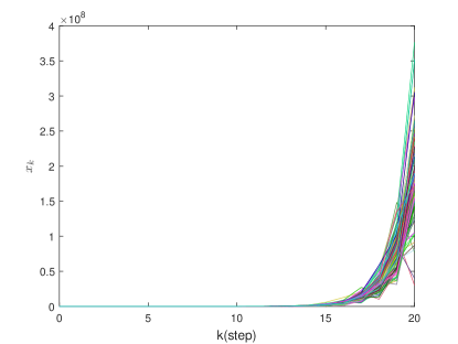
Figure 1: $x_{k}$ of the open-loop system (54).

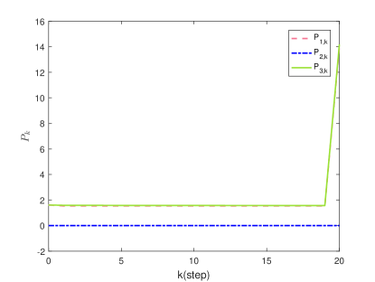
Figure 2: Feasible solutions $P_{k}$.

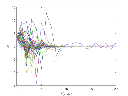
Figure 3: $x_{k}$ of the closed-loop system (54).

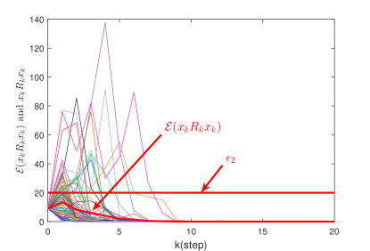
Figure 4: $x_{k}^{\prime}Rx_{k}$ and $\mathcal{E}(x_{k}^{\prime}Rx_{k})$ of the closed-loop system (54).

In the sequel, we present an application to the price control problem of a company’s stock market, which is proposed by [6, 17]. In addition to being adjusted by major shareholders, the stock market is also affected by market fluctuations, changes in crude oil prices, and the average behavior and collective forecast of the stock market. The deviation between the stock market price and the expected price trajectory is described by the following linear discrete mean-field system

$$\begin{cases}x_{k+1}=&A_{1}x_{k}+A_{2}\mathcal{E}x_{k}+Bu_{k}^{F}\\ &+(C_{1}x_{k}+C_{2}\mathcal{E}x_{k}+Du_{k}^{F})w_{k},\end{cases}$$ (54)

where the state $x_{k}$ represents the deviation between the real stock price and the expected value, and the mean term $\mathcal{E}x_{k}$ stands for the average impact of collective forecasting on the stock market. The noise $w_{k}$ can be regarded as the unpredictable influence caused by the continuous fluctuation of unemployment rate and other random events. $u_{k}$ represents the investment and adjustment of the company’s production activities, but due to the unreasonable organizational structure or internal corruption, the final investment or strategy adjustment is $u_{k}^{F}$. If the company expects to keep the deviation within the allowable range within $20$ trading days. We can achieve this goal by the idea of non-fragile finite-time stabilization.

If the parameters of the system (54) are $A_{1}=1.1833$, $A_{2}=1.2741$, $B=-1.3517$, $C_{1}=0.8188$, $C_{2}=-0.1491$, $D=-0.54$, $M=-0.1005$, $N_{1}=-0.6177$, $N_{2}=0.4285$, and $x_{0}=3$. Fig. 1 shows the open-loop state trajectory of $100$ repeated simulations of system (54). Set $\{R_{k}=e^{-0.1\times k}\}_{k\in{\mathcal{N}}_{20}}$, $\epsilon_{1}=10$, $\epsilon_{2}=20$, $T=20$, $\gamma=0.5086$. By Theorem 4.6, we can obtain the control gain parameters $K_{1}=0.9627$ and $K_{2}=0.7737$. Feasible solutions $P_{k}=\left[\begin{array}[]{cc}P_{1,k}&P_{2,k}\\ P_{2,k}&P_{3,k}\end{array}\right]$ are presented in Fig. 2. The corresponding state response of system (54) with control $u_{k}^{F}$ is depicted in Fig. 3. The result is confirmed by the time evolution of $\mathcal{E}(x_{k}^{\prime}R_{k}x_{k})$ of the closed-loop system (54) presented in Fig. 4.

6 Conclusion

Several kinds of STMs of LDMFS systems have been firstly presented in this paper and the non-fragile finite-time stabilization problem has been studied. Based on the STM method, several necessary and sufficient conditions for non-fragile finite-time stabilization have been derived. The advantage of the STM method is non-conservative. The feasibility and effectiveness of the new design schemes have been confirmed by one example. We believe that the STM method will have more applications in stochastic stability and stabilization, which merits further study in our future work.

7 Appendix

The proof of Lemma 3.1:

This lemma can be shown by induction. For any $k$, if $l=k+1$, (10) is evidently valid. Suppose that (10) holds for $l=k+m$, i.e.,

$$\left[\begin{array}[]{cccc}\psi_{k+m,k+1}(\sqrt{\bar{\alpha}}\mathcal{A}_{1,k}+\sqrt{\bar{\alpha}}\mathcal{A}_{2,k})\\ \psi_{k+m,k+1}\sqrt{1-\bar{\alpha}}\mathcal{A}_{1,k}\\ \psi_{k+m,k+1}(\sqrt{\bar{\alpha}}\mathcal{C}_{1}+\sqrt{\bar{\alpha}}\mathcal{C}_{2,k})\\ \psi_{k+m,k+1}\sqrt{1-\bar{\alpha}}\mathcal{C}_{1}\\ \end{array}\right]$$ (59)

$$= \left(I_{4^{m-1}}\otimes\left[\begin{array}[]{cccc}\sqrt{\bar{\alpha}}\mathcal{A}_{1,k+m-1}+\sqrt{\bar{\alpha}}\mathcal{A}_{2,k+m-1}\\ \sqrt{1-\bar{\alpha}}\mathcal{A}_{1,k+m-1}\\ \sqrt{\bar{\alpha}}\mathcal{C}_{1}+\sqrt{\bar{\alpha}}\mathcal{C}_{2,k+m-1}\\ \sqrt{1-\bar{\alpha}}\mathcal{C}_{1}\end{array}\right]\right)\varphi_{k+m-1,k}.$$ (64)

Then, we verify the case of $l=k+m+1$. By definition,

$$\psi_{k+m+1,k}=\left[\begin{array}[]{cccc}\psi_{k+m+1,k+1}(\sqrt{\bar{\alpha}}\mathcal{A}_{1,k}+\sqrt{\bar{\alpha}}\mathcal{A}_{2,k})\\ \psi_{k+m+1,k+1}\sqrt{1-\bar{\alpha}}\mathcal{A}_{1,k}\\ \psi_{k+m+1,k+1}(\sqrt{\bar{\alpha}}\mathcal{C}_{1}+\sqrt{\bar{\alpha}}\mathcal{C}_{2,k})\\ \psi_{k+m+1,k+1}\sqrt{1-\bar{\alpha}}\mathcal{C}_{1}\\ \end{array}\right].$$

Because of the arbitrariness of $k$, we have $\psi_{k+m+1,k+1}=\varphi_{k+m+1,k+1}.$ Therefore,

$$\psi_{k+m+1,k}$$

$$= \left(I_{4}\otimes\left[I_{4^{m-1}}\otimes\left[\begin{array}[]{cccc}\sqrt{\bar{\alpha}}\mathcal{A}_{1,k+m}+\sqrt{\bar{\alpha}}\mathcal{A}_{2,k+m}\\ \sqrt{1-\bar{\alpha}}\mathcal{A}_{1,k+m}\\ \sqrt{\bar{\alpha}}\mathcal{C}_{1}+\sqrt{\bar{\alpha}}\mathcal{C}_{2,k+m}\\ \sqrt{1-\bar{\alpha}}\mathcal{C}_{1}\end{array}\right]\right]\right)$$

$$\left[\begin{array}[]{ccc}\varphi_{k+m,k+1}(\sqrt{\bar{\alpha}}\mathcal{A}_{1,k}+\sqrt{\bar{\alpha}}\mathcal{A}_{2,k})\\ \varphi_{k+m,k+1}\sqrt{1-\bar{\alpha}}\mathcal{A}_{1,k}\\ \varphi_{k+m,k+1}(\sqrt{\bar{\alpha}}\mathcal{C}_{1}+\sqrt{\bar{\alpha}}\mathcal{C}_{2,k})\\ \varphi_{k+m,k+1}\sqrt{1-\bar{\alpha}}\mathcal{C}_{1}\end{array}\right]$$

$$= \left(I_{4^{m}}\otimes\left[\begin{array}[]{cccc}\sqrt{\bar{\alpha}}\mathcal{A}_{1,k+m}+\sqrt{\bar{\alpha}}\mathcal{A}_{2,k+m}\\ \sqrt{1-\bar{\alpha}}\mathcal{A}_{1,k+m}\\ \sqrt{\bar{\alpha}}\mathcal{C}_{1}+\sqrt{\bar{\alpha}}\mathcal{C}_{2,k+m}\\ \sqrt{1-\bar{\alpha}}\mathcal{C}_{1}\end{array}\right]\right)\psi_{k+m,k}.$$

So (10) is proved. $\square$

The proof of Lemma 3.2:

We first prove (12). Because $\alpha_{k}$ and $x_{k}$ are independent of each other, for $k=l-1$, we have

$$\mathcal{E}\|\tilde{x}_{l}\|^{2}=\mathcal{E}\big{[}\big{(}\tilde{A}_{k}\tilde{x}_{k}+\tilde{C}_{k}\tilde{x}_{k}w_{k}\big{)}^{\prime}\big{(}\tilde{A}_{k}\tilde{x}_{k}+\tilde{C}_{k}\tilde{x}_{k}w_{k}\big{)}\big{]}$$

$$= \mathcal{E}\big{\{}\big{[}(\mathcal{A}_{1,k}+\alpha_{k}\mathcal{A}_{2,k})\tilde{x}_{k}+(\mathcal{C}_{1}+\alpha_{k}\mathcal{C}_{2,k})\tilde{x}_{k}w_{k}\big{]}^{\prime}$$

$$\big{[}(\mathcal{A}_{1,k}+\alpha_{k}\mathcal{A}_{2,k})\tilde{x}_{k}+(\mathcal{C}_{1}+\alpha_{k}\mathcal{C}_{2,k})\tilde{x}_{k}w_{k}\big{]}\big{\}}$$

$$= \mathcal{E}\big{[}\tilde{x}_{k}^{\prime}(\mathcal{A}_{1,k}^{\prime}\mathcal{A}_{1,k}+\bar{\alpha}\mathcal{A}_{1,k}^{\prime}\mathcal{A}_{2,k}+\bar{\alpha}\mathcal{A}_{2,k}^{\prime}\mathcal{A}_{1,k}+\bar{\alpha}\mathcal{A}_{2,k}^{\prime}\mathcal{A}_{2,k})\tilde{x}_{k}$$

$$+\tilde{x}_{k}^{\prime}(\mathcal{C}_{1}^{\prime}\mathcal{C}_{1}+\bar{\alpha}\mathcal{C}_{1}^{\prime}\mathcal{C}_{2,k}+\bar{\alpha}\mathcal{C}_{2,k}^{\prime}\mathcal{C}_{1}+\bar{\alpha}\mathcal{C}_{2,k}^{\prime}\mathcal{C}_{2,k})\tilde{x}_{k}\big{]}$$

$$= \mathcal{E}\|\psi_{k+1,k}\tilde{x}_{k}\|^{2}.$$

Hence, equation (12) holds for $k=l-1$. Assume that $\mathcal{E}\|\tilde{x}_{l}\|^{2}=\mathcal{E}\|\psi_{l,k}\tilde{x}_{k}\|^{2}$ holds for $k=l-m$, $1<m<l$. Now we need to prove (12) in the case of $k=l-m-1$. By Lemma 3.1, it can be seen that

$$\mathcal{E}\|\tilde{x}_{l}\|^{2}=\mathcal{E}\|\psi_{l,l-m}\tilde{x}_{l-m}\|^{2}$$

$$= \mathcal{E}\big{[}\tilde{x}_{l-m-1}^{\prime}(\mathcal{A}_{1,l-m-1}^{\prime}\psi_{l,l-m}^{\prime}\psi_{l,l-m}\mathcal{A}_{1,l-m-1}$$

$$+\bar{\alpha}\mathcal{A}_{1,l-m-1}^{\prime}\psi_{l,l-m}^{\prime}\psi_{l,l-m}\mathcal{A}_{2,l-m-1}$$

$$+\bar{\alpha}\mathcal{A}_{2,l-m-1}^{\prime}\psi_{l,l-m}^{\prime}\psi_{l,l-m}\mathcal{A}_{1,l-m-1}$$

$$+\bar{\alpha}\mathcal{A}_{2,l-m-1}^{\prime}\psi_{l,l-m}^{\prime}\psi_{l,l-m}\mathcal{A}_{2,l-m-1})\tilde{x}_{l-m-1}$$

$$+\tilde{x}_{l-m-1}^{\prime}(\mathcal{C}_{1}^{\prime}\psi_{l,l-m}^{\prime}\psi_{l,l-m}\mathcal{C}_{1}+\bar{\alpha}\mathcal{C}_{1}^{\prime}\psi_{l,l-m}^{\prime}\psi_{l,l-m}\mathcal{C}_{2,l-m-1}$$

$$+\bar{\alpha}\mathcal{C}_{2,l-m-1}^{\prime}\psi_{l,l-m}^{\prime}\psi_{l,l-m}\mathcal{C}_{1}+\bar{\alpha}\mathcal{C}_{2,l-m-1}^{\prime}\psi_{l,l-m}^{\prime}\psi_{l,l-m}$$

$$\cdot\mathcal{C}_{2,l-m-1})\tilde{x}_{l-m-1}\big{]}$$

$$= \mathcal{E}\|\psi_{l,l-m-1}\tilde{x}_{l-m-1}\|^{2}.$$

So (12) is shown. Finally, we prove (13). By (10), we have

$$\psi_{l,k}= \left[\begin{array}[]{cccc}\psi_{l,k+1}(\sqrt{\bar{\alpha}}\mathcal{A}_{1,k}+\sqrt{\bar{\alpha}}\mathcal{A}_{2,k})\\ \psi_{l,k+1}\sqrt{1-\bar{\alpha}}\mathcal{A}_{1,k}\\ \psi_{l,k+1}(\sqrt{\bar{\alpha}}\mathcal{C}_{1}+\sqrt{\bar{\alpha}}\mathcal{C}_{2,k})\\ \psi_{l,k+1}\sqrt{1-\bar{\alpha}}\mathcal{C}_{1}\\ \end{array}\right]$$

$$= \left(I_{4^{l-k-1}}\otimes\left[\begin{array}[]{cccc}\sqrt{\bar{\alpha}}\mathcal{A}_{1,l-1}+\sqrt{\bar{\alpha}}\mathcal{A}_{2,l-1}\\ \sqrt{1-\bar{\alpha}}\mathcal{A}_{1,l-1}\\ \sqrt{\bar{\alpha}}\mathcal{C}_{1}+\sqrt{\bar{\alpha}}\mathcal{C}_{2,l-1}\\ \sqrt{1-\bar{\alpha}}\mathcal{C}_{1}\end{array}\right]\right)\psi_{l-1,k}.$$

Note that there must exist elementary matrices $P_{l,k}\in\mathcal{R}^{(4^{l-k}2n)\times(4^{l-k}2n)}$ and $P_{l-1,k}\in\mathcal{R}^{(4^{l-k-1}2n)\times(4^{l-k-1}2n)}$ with $P_{l,k}^{\prime}P_{l,k}=I_{4^{l-k}2n}$ and $P_{l-1,k}^{\prime}P_{l-1,k}=I_{4^{l-k-1}2n}$, such that

$$I_{4^{l-k-1}}\otimes\left[\begin{array}[]{cccc}\sqrt{\bar{\alpha}}\mathcal{A}_{1,l-1}+\sqrt{\bar{\alpha}}\mathcal{A}_{2,l-1}\\ \sqrt{1-\bar{\alpha}}\mathcal{A}_{1,l-1}\\ \sqrt{\bar{\alpha}}\mathcal{C}_{1}+\sqrt{\bar{\alpha}}\mathcal{C}_{2,l-1}\\ \sqrt{1-\bar{\alpha}}\mathcal{C}_{1}\end{array}\right]$$

$$= P_{l,k}^{-1}\left[\begin{array}[]{cc}I_{4^{l-k-1}}\otimes(\sqrt{\bar{\alpha}}\mathcal{A}_{1,l-1}+\sqrt{\bar{\alpha}}\mathcal{A}_{2,l-1})\\ I_{4^{l-k-1}}\otimes\sqrt{1-\bar{\alpha}}\mathcal{A}_{1,l-1}\\ I_{4^{l-k-1}}\otimes(\sqrt{\bar{\alpha}}\mathcal{C}_{1}+\sqrt{\bar{\alpha}}\mathcal{C}_{2,l-1})\\ I_{4^{l-k-1}}\otimes\sqrt{1-\bar{\alpha}}\mathcal{C}_{1}\\ \end{array}\right]P_{l-1,k}.$$

From (12), we can get that

$$\psi_{l,k}=\left(I_{4^{l-k-1}}\otimes\left[\begin{array}[]{cccc}\sqrt{\bar{\alpha}}\mathcal{A}_{1,l-1}+\sqrt{\bar{\alpha}}\mathcal{A}_{2,l-1}\\ \sqrt{1-\bar{\alpha}}\mathcal{A}_{1,l-1}\\ \sqrt{\bar{\alpha}}\mathcal{C}_{1}+\sqrt{\bar{\alpha}}\mathcal{C}_{2,l-1}\\ \sqrt{1-\bar{\alpha}}\mathcal{C}_{1}\end{array}\right]\right)\psi_{l-1,k}$$

$$\Rightarrow \psi_{l,k}=P_{l,k}^{-1}\left[\begin{array}[]{cc}I_{4^{l-k-1}}\otimes(\sqrt{\bar{\alpha}}\mathcal{A}_{1,l-1}+\sqrt{\bar{\alpha}}\mathcal{A}_{2,l-1})\\ I_{4^{l-k-1}}\otimes\sqrt{1-\bar{\alpha}}\mathcal{A}_{1,l-1}\\ I_{4^{l-k-1}}\otimes(\sqrt{\bar{\alpha}}\mathcal{C}_{1}+\sqrt{\bar{\alpha}}\mathcal{C}_{2,l-1})\\ I_{4^{l-k-1}}\otimes\sqrt{1-\bar{\alpha}}\mathcal{C}_{1}\\ \end{array}\right]$$

$$\ \ \ \ \ \ \ \ \ \cdot P_{l-1,k}\psi_{l-1,k}$$

$$\Rightarrow P_{l,k}\psi_{l,k}=\left[\begin{array}[]{cc}I_{4^{l-k-1}}\otimes(\sqrt{\bar{\alpha}}\mathcal{A}_{1,l-1}+\sqrt{\bar{\alpha}}\mathcal{A}_{2,l-1})\\ I_{4^{l-k-1}}\otimes\sqrt{1-\bar{\alpha}}\mathcal{A}_{1,l-1}\\ I_{4^{l-k-1}}\otimes(\sqrt{\bar{\alpha}}\mathcal{C}_{1}+\sqrt{\bar{\alpha}}\mathcal{C}_{2,l-1})\\ I_{4^{l-k-1}}\otimes\sqrt{1-\bar{\alpha}}\mathcal{C}_{1}\\ \end{array}\right]$$

$$\ \ \ \ \ \ \ \ \ \ \ \ \ \cdot P_{l-1,k}\psi_{l-1,k}.$$

Set $\phi_{l,k}=P_{l,k}\psi_{l,k}$, then (13) is proved. $\square$

The proof of Lemma 3.3:

Note that $R_{k+1}$ and $R_{k}$ are given positive definite matrices. It is easy to see that

$$\bar{x}_{k+1}=\bar{R}_{k+1}^{\frac{1}{2}}\tilde{x}_{k+1}$$

$$= (\bar{R}_{k+1}^{\frac{1}{2}}\mathcal{A}_{1,k}\mathcal{R}_{k}^{-\frac{1}{2}}+\alpha_{k}\bar{R}_{k+1}^{\frac{1}{2}}\mathcal{A}_{2,k}\bar{R}_{k}^{-\frac{1}{2}})\bar{x}_{k}$$

$$+(\bar{R}_{k+1}^{\frac{1}{2}}\mathcal{C}_{1}\bar{R}_{k}^{-\frac{1}{2}}+\alpha_{k}\bar{R}_{k+1}^{\frac{1}{2}}\mathcal{C}_{2,k}\bar{R}_{k}^{-\frac{1}{2}})\bar{x}_{k}w_{k}.$$

So the dynamic system of $\bar{x}_{k}$ is obtained. The STM $\bar{\phi}_{l,k}$ can be given via Lemma 3.2, so can $\bar{\psi}_{l,k}$. The proof is completed. $\square$

The proof of Lemma 3.4:

By Lemma 2.1, $I_{4^{l-k}}\otimes\bar{R}_{l}$ can be broken down into $(I_{4^{l-k}}\otimes\bar{R}_{l}^{\frac{1}{2}})(I_{4^{l-k}}\otimes\bar{R}_{l}^{\frac{1}{2}})$. So, the problem reduces into proving the following equation:

$$(I_{4^{l-k}}\otimes\bar{R}_{l}^{\frac{1}{2}})\phi_{l,k}=\bar{\phi}_{l,k}\bar{R}_{k}^{\frac{1}{2}}.$$ (65)

For $l=k$, in view of $\phi_{k,k}=\bar{\phi}_{k,k}=I_{2n}$, we have $(I_{1}\otimes\bar{R}_{k}^{\frac{1}{2}})\phi_{k,k}=\bar{R}_{k}^{\frac{1}{2}}=\bar{\phi}_{k,k}\bar{R}_{k}^{\frac{1}{2}}.$ Hence, (65) holds for $l=k$. We suppose (65) holds when $l=k+i-1$, i.e., $(I_{4^{i-1}}\otimes\bar{R}_{k+i-1}^{\frac{1}{2}})\phi_{k+i-1,k}=\bar{\phi}_{k+i-1,k}\bar{R}_{k}^{\frac{1}{2}}$, then only the equation $(I_{4^{i}}\otimes\bar{R}_{k+i}^{\frac{1}{2}})\phi_{k+i,k}=\bar{\phi}_{k+i,k}\bar{R}_{k}^{\frac{1}{2}}$ needs to be proved. By Lemma 2.1, it can be seen that

$$(I_{4^{i}}\otimes\bar{R}_{k+i}^{\frac{1}{2}})\phi_{k+i,k}$$

$$= \left[\begin{array}[]{cccc}(I_{4^{i-1}}\otimes(\sqrt{\bar{\alpha}}\bar{R}_{k+i}\mathcal{A}_{1,k+i-1}+\sqrt{\bar{\alpha}}\bar{R}_{k+i}\mathcal{A}_{2,k+i-1}))\phi_{k+i-1,k}\\ (I_{4^{i-1}}\otimes\sqrt{1-\bar{\alpha}}\bar{R}_{k+i}\mathcal{A}_{1,k+i-1})\phi_{k+i-1,k}\\ (I_{4^{i-1}}\otimes(\sqrt{\bar{\alpha}}\bar{R}_{k+i}\mathcal{C}_{1}+\sqrt{\bar{\alpha}}\bar{R}_{k+i}\mathcal{C}_{2,k+i-1}))\phi_{k+i-1,k}\\ (I_{4^{i-1}}\otimes\sqrt{1-\bar{\alpha}}\bar{R}_{k+i}\mathcal{C}_{1})\phi_{k+i-1,k}\end{array}\right]$$

$$= \left[\begin{array}[]{cccc}\Theta_{1}^{\prime}&\Theta_{2}^{\prime}&\Theta_{3}^{\prime}&\Theta_{4}^{\prime}\end{array}\right]^{\prime}$$

$$= \bar{\phi}_{k+i,k}\bar{R}_{k}^{\frac{1}{2}},$$

where

$$\Theta_{1}= (I_{4^{i-1}}\otimes(\sqrt{\bar{\alpha}}\bar{R}_{k+i}\mathcal{A}_{1,k+i-1}+\sqrt{\bar{\alpha}}\bar{R}_{k+i}\mathcal{A}_{2,k+i-1}))$$

$$\cdot(I_{4^{i-1}}\otimes\bar{R}_{k+i-1}^{-\frac{1}{2}})(I_{4^{i-1}}\otimes\bar{R}_{k+i-1}^{\frac{1}{2}})\phi_{k+i-1,k},$$

$$\Theta_{2}= (I_{4^{i-1}}\otimes(\sqrt{1-\bar{\alpha}}\bar{R}_{k+i}\mathcal{A}_{1,k+i-1}))(I_{4^{i-1}}\otimes\bar{R}_{k+i-1}^{-\frac{1}{2}})$$

$$\cdot(I_{4^{i-1}}\otimes\bar{R}_{k+i-1}^{\frac{1}{2}})\phi_{k+i-1,k},$$

$$\Theta_{3}= (I_{4^{i-1}}\otimes(\sqrt{\bar{\alpha}}\bar{R}_{k+i}\mathcal{C}_{1}+\sqrt{\bar{\alpha}}\bar{R}_{k+i}\mathcal{C}_{2,k+i-1}))(I_{4^{i-1}}\otimes\bar{R}_{k+i-1}^{-\frac{1}{2}})$$

$$\cdot(I_{4^{i-1}}\otimes\bar{R}_{k+i-1}^{\frac{1}{2}})\phi_{k+i-1,k},$$

$$\Theta_{4}= (I_{4^{i-1}}\otimes(\sqrt{1-\bar{\alpha}}\bar{R}_{k+i}\mathcal{C}_{1}))(I_{4^{i-1}}\otimes\bar{R}_{k+i-1}^{-\frac{1}{2}})(I_{4^{i-1}}\otimes\bar{R}_{k+i-1}^{\frac{1}{2}})$$

$$\cdot\phi_{k+i-1,k}.$$

This completes the proof. $\square$

The proof of Lemma 3.5:

We also use the induction principle to prove the lemma. Obviously, in the case of $k=l$, (15) is right. Suppose that for $k=i<l$, (15) holds, i.e., $\psi^{\prime}_{l,i}(I_{4^{l-i}}\otimes\bar{R}_{l})\psi_{l,i}=\bar{R}_{i}^{\frac{1}{2}}\bar{\psi}^{\prime}_{l,i}\bar{\psi}_{l,i}\bar{R}_{i}^{\frac{1}{2}}.$ Then we only need to show $\psi^{\prime}_{l,i-1}(I_{4^{l-i+1}}\otimes\bar{R}_{l})\psi_{l,i-1}=\bar{R}_{i-1}^{\frac{1}{2}}\bar{\psi}^{\prime}_{l,i-1}\bar{\psi}_{l,i-1}\bar{R}_{i-1}^{\frac{1}{2}}.$ The right hand side of the above equation can be computed as

$$\bar{R}_{i-1}^{\frac{1}{2}}\bar{\psi}^{\prime}_{l,i-1}\bar{\psi}_{l,i-1}\bar{R}_{i-1}^{\frac{1}{2}}$$

$$= \bar{R}_{i-1}^{\frac{1}{2}}\left[\begin{array}[]{cccc}\bar{\psi}_{l,i}(\sqrt{\bar{\alpha}}\bar{R}_{i}^{\frac{1}{2}}\mathcal{A}_{1,i-1}\bar{R}_{i-1}^{-\frac{1}{2}}+\sqrt{\bar{\alpha}}\bar{R}_{i}^{\frac{1}{2}}\mathcal{A}_{2,i-1}\bar{R}_{i-1}^{-\frac{1}{2}})\\ \bar{\psi}_{l,i}(\sqrt{1-\bar{\alpha}}\bar{R}_{i}^{\frac{1}{2}}\mathcal{A}_{1,i-1}\bar{R}_{i-1}^{-\frac{1}{2}})\\ \bar{\psi}_{l,i}(\sqrt{\bar{\alpha}}\bar{R}_{i}^{\frac{1}{2}}\mathcal{C}_{1}\bar{R}_{i-1}^{-\frac{1}{2}}+\sqrt{\bar{\alpha}}\bar{R}_{i}^{\frac{1}{2}}\mathcal{C}_{2,i-1}\bar{R}_{i-1}^{-\frac{1}{2}})\\ \bar{\psi}_{l,i}(\sqrt{1-\bar{\alpha}}\bar{R}_{i}^{\frac{1}{2}}\mathcal{C}_{1}\bar{R}_{i-1}^{-\frac{1}{2}})\\ \end{array}\right]^{\prime}$$

$$\cdot\left[\begin{array}[]{cccc}\bar{\psi}_{l,i}(\sqrt{\bar{\alpha}}\bar{R}_{i}^{\frac{1}{2}}\mathcal{A}_{1,i-1}\bar{R}_{i-1}^{-\frac{1}{2}}+\sqrt{\bar{\alpha}}\bar{R}_{i}^{\frac{1}{2}}\mathcal{A}_{2,i-1}\bar{R}_{i-1}^{-\frac{1}{2}})\\ \bar{\psi}_{l,i}(\sqrt{1-\bar{\alpha}}\bar{R}_{i}^{\frac{1}{2}}\mathcal{A}_{1,i-1}\bar{R}_{i-1}^{-\frac{1}{2}})\\ \bar{\psi}_{l,i}(\sqrt{\bar{\alpha}}\bar{R}_{i}^{\frac{1}{2}}\mathcal{C}_{1}\bar{R}_{i-1}^{-\frac{1}{2}}+\sqrt{\bar{\alpha}}\bar{R}_{i}^{\frac{1}{2}}\mathcal{C}_{2,i-1}\bar{R}_{i-1}^{-\frac{1}{2}})\\ \bar{\psi}_{l,i}(\sqrt{1-\bar{\alpha}}\bar{R}_{i}^{\frac{1}{2}}\mathcal{C}_{1}\bar{R}_{i-1}^{-\frac{1}{2}})\\ \end{array}\right]\bar{R}_{i-1}^{\frac{1}{2}}$$

$$= \left[\begin{array}[]{cccc}\bar{\psi}_{l,i}(\sqrt{\bar{\alpha}}\bar{R}_{i}^{\frac{1}{2}}\mathcal{A}_{1,i-1}+\sqrt{\bar{\alpha}}\bar{R}_{i}^{\frac{1}{2}}\mathcal{A}_{2,i-1})\\ \bar{\psi}_{l,i}(\sqrt{1-\bar{\alpha}}\bar{R}_{i}^{\frac{1}{2}}\mathcal{A}_{1,i-1})\\ \bar{\psi}_{l,i}(\sqrt{\bar{\alpha}}\bar{R}_{i}^{\frac{1}{2}}\mathcal{C}_{1}+\sqrt{\bar{\alpha}}\bar{R}_{i}^{\frac{1}{2}}\mathcal{C}_{2,i-1})\\ \bar{\psi}_{l,i}(\sqrt{1-\bar{\alpha}}\bar{R}_{i}^{\frac{1}{2}}\mathcal{C}_{1})\\ \end{array}\right]^{\prime}$$

$$\cdot\left[\begin{array}[]{cccc}\bar{\psi}_{l,i}(\sqrt{\bar{\alpha}}\bar{R}_{i}^{\frac{1}{2}}\mathcal{A}_{1,i-1}+\sqrt{\bar{\alpha}}\bar{R}_{i}^{\frac{1}{2}}\mathcal{A}_{2,i-1})\\ \bar{\psi}_{l,i}(\sqrt{1-\bar{\alpha}}\bar{R}_{i}^{\frac{1}{2}}\mathcal{A}_{1,i-1})\\ \bar{\psi}_{l,i}(\sqrt{\bar{\alpha}}\bar{R}_{i}^{\frac{1}{2}}\mathcal{C}_{1}+\sqrt{\bar{\alpha}}\bar{R}_{i}^{\frac{1}{2}}\mathcal{C}_{2,i-1})\\ \bar{\psi}_{l,i}(\sqrt{1-\bar{\alpha}}\bar{R}_{i}^{\frac{1}{2}}\mathcal{C}_{1})\\ \end{array}\right]$$

$$= \psi^{\prime}_{l,i-1}(I_{4^{l-i+1}}\otimes\bar{R}_{i})\psi_{l,i-1}.$$

This lemma is proved. $\square$

The proof of Theorem 3.1:

We first prove (b)$\Rightarrow$(a) in Theorem 3.1. By Lemma 3.3, LDMFS system (2) is finite-time stabilizable with respect to $(\epsilon_{1},\epsilon_{2},T,\{R_{k}\}_{k\in{\mathcal{N}}_{T}})$ iff the system (14) is finite-time stable with respect to $(\epsilon_{1},\epsilon_{2},T,\{I_{2n})\}$. If

$$x_{0}^{\prime}R_{0}x_{0}\leq\epsilon_{1},$$ (66)

then, by Lemma 3.4, we have

$$\mathcal{E}(x_{k}^{\prime}R_{k}x_{k})= \bar{x}^{\prime}_{0}\bar{\phi}^{\prime}_{k,0}\bar{\phi}_{k,0}\bar{x}_{0}=\tilde{x}_{0}^{\prime}\bar{R}_{0}^{\frac{1}{2}}\bar{\phi}^{\prime}_{k,0}\bar{\phi}_{k,0}\bar{R}_{0}^{\frac{1}{2}}\tilde{x}_{0}$$

$$= \tilde{x}_{0}^{\prime}\phi^{\prime}_{k,0}(I_{4^{k}}\otimes\bar{R}_{k})\phi_{k,0}\tilde{x}_{0}.$$ (67)

When $x_{0}=0$, it directly leads to $\mathcal{E}(x_{k}^{\prime}Rx_{k})\equiv 0<\epsilon_{2}$. When $x_{0}\neq 0$, by (66) and (7), we obtain $\mathcal{E}(x_{k}^{\prime}R_{k}x_{k})\leq\tilde{x}_{0}^{\prime}\frac{\epsilon_{2}}{\epsilon_{1}}\bar{R}_{0}\tilde{x}_{0}\leq\epsilon_{2},k\in{\mathcal{N}}_{T}.$ All in all, for any $x_{0}\in\mathcal{R}^{n}$ satisfying (66), it can be always concluded that $\mathcal{E}(x_{k}^{\prime}R_{k}x_{k})\leq\epsilon_{2}$. Thus (a) holds.

(a)$\Rightarrow$(b): In the case of that system (2) is finite-time stabilizable with respect to $(\epsilon_{1},\epsilon_{2},T,\{R_{k}\}_{k\in{\mathcal{N}}_{T}})$, (16) must hold, otherwise, there exist $k_{0}\in\mathcal{N}_{T}$ and $\tilde{x}_{0}$ with $\tilde{x}_{0}^{\prime}\bar{R}_{0}\tilde{x}_{0}=\epsilon_{1}$, such that

$$\mathcal{E}(\tilde{x}_{k_{0}}^{\prime}\bar{R}_{k_{0}}\tilde{x}_{k_{0}})=\tilde{x}_{0}^{\prime}\phi_{k_{0},0}^{\prime}(I_{4^{k_{0}}}\otimes\bar{R}_{k_{0}})\phi_{k_{0},0}\tilde{x}_{0}\geq\tilde{x}_{0}^{\prime}\frac{\epsilon_{2}}{\epsilon_{1}}\tilde{x}_{0}\geq\epsilon_{2}.$$

This contradicts the definition of finite-time stability. Therefore, (b) is derived.

By considering Lemma 3.4 and (b), we can get that $\phi^{\prime}_{k,0}(I_{4^{k}}\otimes\bar{R}_{k})\phi_{k,0}=\bar{R}_{0}^{\frac{1}{2}}\bar{\phi}^{\prime}_{k,0}\bar{\phi}_{k,0}\bar{R}_{0}^{\frac{1}{2}}$. Therefore (b)$\Leftrightarrow$(c). Analogously, according to Lemmas 3.4 and 3.5, it follows that (a)$\Leftrightarrow$(d)$\Leftrightarrow$(e).

(b)$\Leftrightarrow$(f): By Lemma 2.1 and $\bar{R}_{k}>0$, we have $I_{4^{k}}\otimes\bar{R}_{k}=(I_{4^{k}}\otimes\bar{R}_{k}^{1/2})(I_{4^{k}}\otimes\bar{R}_{k}^{1/2})$, where $\bar{R}_{k}^{1/2}>0$. Considering (b), it can be obtained that

$$\phi_{k,0}^{\prime}(I_{4^{k}}\otimes\bar{R}_{k})\phi_{k,0}\leq\frac{\epsilon_{2}}{\epsilon_{1}}\bar{R}_{0}$$

$$\Leftrightarrow \phi_{k,0}^{\prime}(I_{4^{k}}\otimes\bar{R}_{k}^{1/2})(I_{4^{k}}\otimes\bar{R}_{k}^{1/2})\phi_{k,0}\leq\frac{\epsilon_{2}}{\epsilon_{1}}\bar{R}_{0}$$

$$\Leftrightarrow \bar{R}_{0}^{-1/2}\phi_{k,0}^{\prime}(I_{4^{k}}\otimes\bar{R}_{k}^{1/2})(I_{4^{k}}\otimes\bar{R}_{k}^{1/2})\phi_{k,0}\bar{R}_{0}^{-1/2}\leq\frac{\epsilon_{2}}{\epsilon_{1}}I_{2n}.$$

Through Schur’s complement lemma, the above relationship yields that

$$\left[\begin{array}[]{ccccc}-\frac{\epsilon_{2}}{\epsilon_{1}}I_{2n}&\bar{R}_{0}^{-1/2}\phi_{k,0}^{\prime}(I_{4^{k}}\otimes\bar{R}_{k}^{1/2})\\ (I_{4^{k}}\otimes\bar{R}_{k}^{1/2})\phi_{k,0}\bar{R}_{0}^{-1/2}&-I_{4^{k}\times 2n}\end{array}\right]\leq 0$$

$$\Leftrightarrow [(I_{4^{k}}\otimes\bar{R}_{k}^{1/2})\phi_{k,0}\bar{R}_{0}^{-1/2}][\bar{R}_{0}^{-1/2}\phi^{\prime}_{k,0}(I_{4^{k}}\otimes\bar{R}_{k}^{1/2})]$$

$$-\frac{\epsilon_{2}}{\epsilon_{1}}I_{4^{k}\times 2n}\leq 0.$$

Set $P_{k}=\phi_{k,0}\bar{R}_{0}^{-1}\phi^{\prime}_{k,0}$, then (b) is equivalent to

$$(I_{4^{k}}\otimes\bar{R}_{k}^{1/2})P_{k}(I_{4^{k}}\otimes\bar{R}_{k}^{1/2})-\frac{\epsilon_{2}}{\epsilon_{1}}I_{4^{k}\times 2n}\leq 0.$$ (68)

Pre-multiplying and post-multiplying (68) by $(I_{4^{k}}\otimes\bar{R}_{k}^{-1/2})=(I_{4^{k}}\otimes\bar{R}_{k}^{-1/2})^{\prime}$, it can be seen that (68) is equivalent to $P_{k}-\frac{\epsilon_{2}}{\epsilon_{1}}(I_{4^{k}}\otimes\bar{R}_{k}^{-1})\leq 0.$ In addition, by the definition of $P_{k}$, it is obvious that $P_{0}=\bar{R}_{0}^{-1}$. Hence, in order to show (b)$\Leftrightarrow$(f), we only need to show that $P_{k}$ satisfies

$$P_{k+1}= \left[\begin{array}[]{cccccc}I_{4^{k}}\otimes(\sqrt{\bar{\alpha}}\mathcal{A}_{1,k}+\sqrt{\bar{\alpha}}\mathcal{A}_{2,k})\\ I_{4^{k}}\otimes\sqrt{1-\bar{\alpha}}\mathcal{A}_{1,k}\\ I_{4^{k}}\otimes(\sqrt{\bar{\alpha}}\mathcal{C}_{1}+\sqrt{\bar{\alpha}}\mathcal{C}_{2,k})\\ I_{4^{k}}\otimes\sqrt{1-\bar{\alpha}}\mathcal{C}_{1}\end{array}\right]P_{k}$$

$$\left[\begin{array}[]{cccccc}I_{4^{k}}\otimes(\sqrt{\bar{\alpha}}\mathcal{A}_{1,k}+\sqrt{\bar{\alpha}}\mathcal{A}_{2,k})\\ I_{4^{k}}\otimes\sqrt{1-\bar{\alpha}}\mathcal{A}_{1,k}\\ I_{4^{k}}\otimes(\sqrt{\bar{\alpha}}\mathcal{C}_{1}+\sqrt{\bar{\alpha}}\mathcal{C}_{2,k})\\ I_{4^{k}}\otimes\sqrt{1-\bar{\alpha}}\mathcal{C}_{1}\end{array}\right]^{\prime},$$

which can be derived by applying the expression of $\phi_{k,0}$ in Lemma 3.2 and the definition of $P_{k}=\phi_{k,0}\bar{R}_{0}^{-1}\phi^{\prime}_{k,0}$. The proof is ended. $\square$

References

• [1] F. Amato, G. De Tommasi, and A. Pironti, “Necessary and sufficient conditions for finite-time stability of impulsive dynamical linear systems,” Automatica, vol. 49, no. 8, pp. 2546–2550, 2013.
• [2] F. Amato, M. Ariola, and C. Cosentino, “Finite-time stability of linear time-varying systems: analysis and controller design,” IEEE Transactions on Automatic Control, vol. 55, no. 4, pp. 1003–1008, 2010.
• [3] F. Amato, R. Ambrosino, M. Ariola, C. Cosentino, and G. D. Tommasi, Finite-Time Stability and Control, London: Springer, 2014.
• [4] B. Acciaio, J. Backhoff-Veraguas, and R. Carmona, “Extended mean field control problems: Stochastic maximum principle and transport perspective,” SIAM Journal on Control and Optimization, vol. 57, pp.3666–3693, 2019.
• [5] W. Chen and J. L. Jiao, “Finite-time stability theorem of stochastic nonlinear systems,” Automatica, vol. 46, pp. 2105–2108, 2010.
• [6] B. S. Chen, C. T. Young, and M. Y. Lee, “Multiplayer noncooperative and cooperative minimax $H_{\infty}$ tracking game strategies for linear mean-field stochastic systems with applications to cyber-social systems,” IEEE Transactions on Cybernetics. vol. 52, no. 5, pp. 2968–2980, 2022.
• [7] R. Elliott, X. Li, and Y. H. Ni, “Discrete time mean-field stochastic linear-quadratic optimal control problems,” Automatica, vol. 49, pp.3222-3233, 2013.
• [8] Y. Hong, Z. Jiang, and G. Feng, “ Finite-time input-to-state stability and applications to finite-time control design,” SIAM Journal on Control and Optimization, vol. 48, pp. 4395–4418, 2010.
• [9] J. Huang and N. Li, “Linear-quadratic mean-field game for stochastic delayed systems,” IEEE Transactions on Automatic Control, vol. 63, pp. 2722–2729, 2018.
• [10] M. Y. Huang, P. E. Caines, and R. P. Malhame, “Large-population cost-coupled LQG problems with nonuniform agents: Individual-mass behavior and decentralized $\varepsilon$-Nash equilibria,” IEEE Transactions on Automatic Control, 52(2017), pp. 1560–1571.
• [11] X. Jiang, S. Tian, T. Zhang, and W. Zhang, Pareto optimal strategy for linear stochastic systems with $H_{\infty}$ constraint in finite horizon, Information Sciences, vol. 512, pp. 1103–1117, 2020.
• [12] X. Jiang, S. Tian, T. Zhang, and W. Zhang, “Stability and stabilization of nonlinear discrete-time stochastic systems,” International Journal of Robust and Nonlinear Control, vol. 29, pp. 6419–6437, 2019.
• [13] S. V. Kumara, S. M. Anthonib, and R. Rajac, “Dissipative analysis for aircraft flight control systems with randomly occurring uncertainties via non-fragile sampled-data control,” Mathematics and Computers in Simulation, vol. 155, pp. 217-226, 2019.
• [14] R. Khasminski, Stochastic Stability of Differential Equations, 2nd Edition, New York: Springer, 2012.
• [15] P. P. Khargonekar, I. R. Petersen, and K. Zhou, “Robust stabilization of uncertain linear systems: quadratic stabilizability and $H_{\infty}$ control theory,” IEEE Transactions on Automatic Control, vol. 35, pp. 356–361, 1990.
• [16] X. Li, X. Yang, and S. Song, “Lyapunov conditions for finite-time stability of time-varying time-delay systems,” Automatica, vol. 103, pp. 135–140, 2019.
• [17] Y. Lin, X. Jiang, and W. Zhang, “An open-loop Stackelberg strategy for the linear quadratic mean-field stochastic differential game,” IEEE Transactions on Automatic Control, vol. 64, no. 1, pp. 97–110, 2019.
• [18] X. Mao, Stochastic Differential Equations and Applications, 2nd Edition, Chichester: Horwood, 2007.
• [19] L. Ma, W. Zhang, and Y. Zhao, “Study on stability and stabilizability of discrete-time mean-field stochastic systems,” Journal of The Franklin Institute, vol. 356, pp. 2153-2171, 2019.
• [20] Q. Meng, C. Qian, and Z. Y. Sun, “Finite-time stability control of an electric vehicle under tyre blowout,” Transactions of the Institute of Measurement and Control, vol. 41, pp.1395–1404, 2019.
• [21] M. Nourian, P. E. Caines, R. P. Malhame, and M. Y. Huang, “Mean feld LQG control in leader-follower stochastic multi-agent systems: Likelihood ratio based adaptation,” IEEE Transactions on Automatic Control, vol. 57, pp. 2801–2816, 2012.
• [22] Y. H. Ni, J. F. Zhang, and M. Krstic, “Time-inconsistent mean-field stochastic LQ problem: Open-loop time-consistent control,” IEEE Transactions on Automatic Control, vol. 63, pp. 2771–2786, 2018.
• [23] P. Pickl, “A simple derivation of mean field limits for quantum systems,” Letters in Mathematical Physics, vol. 97, pp. 151–164, 2011.
• [24] J. Song, Y. Niu, and Y. Zou, “Finite-time stabilization via sliding mode control,” IEEE Transactions on Automatic Control, vol. 62, pp. 1478–1483, 2017.
• [25] R. Sakthivel, T. Saravanakumar, Y. K. Ma, and S. M. Anthoni, “Finite-time resilient reliable sampled-data control for fuzzy systems with randomly occurring uncertainties,” Fuzzy Sets and Systems, vol. 329, pp. 1–18, 2017.
• [26] H. Tembine, Q. N. Zhu, and T. Basar, “Risk-sensitive mean-field games,” IEEE Transactions on Automatic Control, vol. 59, pp. 835–850, 2014.
• [27] H. Wang and Q. Zhu, “Finite-time stabilization of high-order stochastic nonlinear systems in strict-feedback form,” Automatica, vol. 54, pp. 284–291, 2015.
• [28] J. Yong, “Linear-quadratic optimal control problems for mean-field stochastic differential equations,” SIAM Journal on Control and Optimization, vol. 51, pp. 2809–2838, 2013.
• [29] J. Yu, P. Shi, J. Liu and C. Lin, “Neuroadaptive finite-time control for nonlinear MIMO systems with input constraint,” IEEE Transactions on Cybernetics, vol. 52. no.7, pp. 6676-6683, 2022.
• [30] Z. Yan, W. Zhang, and G. Zhang, “Finite-time stability and stabilization of Itô stochastic systems with Markovian switching: Mode-dependent parameter approach,” IEEE Transactions on Automatic Control, vol. 60, pp. 2428–2433, 2015.
• [31] J. Yin, S. Khoo, Z. Man, and X. Yu, “Finite-time stability and instability of stochastic nonlinear systems,” Automatica, vol. 47, pp. 1288–1292, 2011.
• [32] X. Yu, J. Yin, and S. Khoo, “Generalized Lyapunov criteria on finite-time stability of stochastic nonlinear systems,” Automatica, vol. 107, pp. 183-189, 2019.
• [33] J. M. Yang and S. W. Kwak, “Resilient corrective control of asynchronous sequential machines against intermittent loss of actuator outputs,” IEEE Transactions on Cybernetics, 10.1109/TCYB.2022.3167483, 2022.
• [34] W. Zha, J. Zhai, S. Fei, and Y. Wang, “Finite-time stabilization for a class of stochastic nonlinear systems via output feedback,” ISA Transactions, vol. 53, pp. 709–716, 2014.
• [35] T. Zhang, F. Deng, and W. Zhang, “Finite-time stability and stabilization of linear discrete time-varying stochastic systems,” Journal of the Franklin Institute, vol. 356, pp. 1247-1267, 2019.
• [36] T. Zhang, F. Deng, and W. Zhang, “Robust $H_{\infty}$ filtering for nonlinear discrete-time stochastic systems,” Automatica, 10.1016/j.automatica.2020.109343, 2021.
• [37] W. Zhang, W. Zheng, and B. S. Chen, “Detectability, observability and Lyapunov-type theorems of linear discrete time-varying stochastic systems with multiplicative noise,” International Journal of Control, vol. 90, pp. 2490-2507, 2017.
• [38] W. Zhang and C. Peng, “Indefinite mean-field stochastic cooperative linear-quadratic dynamic difference game with its application to the network security model, IEEE Transactions on Cybernetics, DOI: 10.1109/TCYB.2021.3070352, 2021.