Unifying turnaround-bounce cosmology in a cyclic universe considering a running vacuum model

Abstract

Among many models which can describe the bouncing cosmology, A matter bounce scenario that is deformed by a running vacuum model of dark energy (RVM-DE) has been interested. In this research, I show that a class of RVM-CDM (cold dark matter) model can also describe a cyclical cosmology in which the universe undergoes cycles of expansion to the contraction phase and vice versa. To this end, following our previous work, I consider one of the most successful class of RVM-CDM model in bouncing cosmology, $\rho_{x}=n_{0}+n_{2}H^{2}+n_{4}H^{4}$, in which the power spectral index gets a red tilt and the running of the spectral index may give a negative value by choosing the appropriate value of parameters ($n_{0},~{}n_{2},~{}n_{4}$), which is consistent with the cosmological observations. It is worthwhile to mention that most matter bounce models do not produce this negative value. However, the main purpose of this article is to investigate the RVM-CDM model in the turnaround phase. Far from the bounce in a phantom expanding universe, the turnaround conditions are investigated before the occurrence of a sudden big rip. By analyzing the Hubble parameter, equation of state parameter, and deceleration parameter around the turnaround, we show that a successful turnaround may occur after an expansion in an interacting case of RVM-CDM by choosing the appropriate value of parameters. A minimum value for the interaction parameter is obtained and also find any relation between other model parameters. Finally, the effect of each parameter on a turnaround is studied, and we see that the transition time from accelerating to decelerating expansion can occur earlier for larger values of interaction parameter. Also, in several graphs, the effect of the second term in DE density, including $H^{2}$, is studied, and we see that by increasing its coefficient, $n_{2}$, the transition point leads to lower values.

I introduction

For centuries, the debate between a cyclical eternal universe and an accidental one, has been the subject of controversy between philosophers and scientists. In the twentieth century, after the introduction of Einstein’s theory of gravity, Tolman Tolman (1934) returned to the hypothesis of a cyclic universe by using a positive spatially curvature cosmology. Since then, many scientists have proposed different models for this type of universe. These models were presented to resolve the problem of big bang theory, which has an avoidable initial singularity of the universe. Furthermore, in many of cosmological dark energy (DE) models, the existence of a far future singularity, called the big rip, has been predicted Caldwell et al. (2003); Nojiri et al. (2012). A cyclic universe must re-collapse before the big rip occurs. The fundamental question is, what physical process causes these cycles?

One of the interesting models of cyclic cosmology to date is the Conformal Cyclic Cosmology ( CCC) model, which was popularized by a Nobel laureate, Roger Penrose, in 2010 in the book: The Cycle of Time Penrose (2011). Penrose group and other cosmologists have written many articles on the evidence of CCC in observations of the cosmic microwave background (CMB) and its anomalies Penrose (2006, 2012); Gurzadyan and Penrose (2011, 2013, 2016); Penrose (2017); An et al. (2020).

Other successful models that have been also considered in cyclic cosmology are: Steinhardt Turok model Steinhardt and Turok (2002); Steinhardt et al. (2002); Steinhardt and Turok (2003); Boyle et al. (2004); Khoury et al. (2004); Steinhardt and Turok (2005); Lehners and Steinhardt (2008, 2013); Ijjas and Steinhardt (2016, 2017, 2018, 2022, 2019), Baum-Frampton model Baum and Frampton (2007); Frampton (2006, 2007); Aref’eva et al. (2009); Frampton and Ludwick (2013); Corianò and Frampton (2019), and Loop quantum cosmology (LQC).

In LQC model, physicists approach the concepts of quantum mechanics and quantum gravity. A non-perturbative regime of quantum gravity based on loop quantum gravity (LQG), may stand out to arise a nonsingular big bounce or big crunch once before tending to singularity, by some matter-energy content or spatial curvature, for various isotropic and anisotropic models Singh (2009). Following the LQG, the cosmologists introduce an LQC theory, based on discrete quantum geometry arising from the non-perturbative quantum geometric effects Ashtekar and Singh (2011). Using LQC, the Friedmann equation is modified by a quadratic of energy density term (with a negative sign), which in turned into standard Friedmann equation, a little far from the big bounce and turnaround points Wilson-Ewing (2013). The Hubble rate is vanished and changed the sign at maximum energy in a finite value of scale factor. The relic gravitational waves from the merging of a large number of black holes in a collapsed phase of the universe in the pre-bounce regime, may be regarded as good evidence of a cyclic universe Gorkavyi (2022).

Among many models of bouncing cosmology, i.e. Pre-Big-Bang Gasperini and Veneziano (1993) or Ekpyrotic type Khoury et al. (2001), string gas cosmology Brandenberger and Vafa (1989); Nayeri et al. (2006) and matter bounce scenario Finelli and Brandenberger (2002), the last one has the most interested in the last decade Lin et al. (2011); Wilson-Ewing (2013); Cai et al. (2013); Lehners and Wilson-Ewing (2015); Cai et al. (2016a, b). Based on observations of Plank 2015 and 2018 Ade et al. (2016a, b, 2015, 2018), the primordial perturbations were adiabatic, almost scale-invariant with a slight red tilt ($n_{s}=0.968\pm 0.006,~{}(68\%~{}CL)$), and that tensor perturbations were small. Also these observations provide a bound for running of spectral index $\alpha_{s}=-0.003\pm 0.007,~{}(68\%~{}CL)$. In particular, some efforts has been made in a quasi-matter, semi-matter, and deformed matter (a matter term mixed by a dark energy component) bouncing cosmology Cai and Wilson-Ewing (2014, 2015); Arab and Khodam-Mohammadi (2018), where in some of which, the problems of previous models have been solved. Although in many models of matter bounce, the power spectral index ($n_{s}$) of cosmological perturbation may be consistent with observations, the sign of running of the spectral index ($\alpha_{s}$) is one of the matter of challenges among the models. In fact, the quantity $\alpha_{s}$ may be considered as a further observational tool that can be used to differentiate between various cosmological scenarios Lehners and Wilson-Ewing (2015). Most recently, in Arab and Khorasani (2021), authors made constraint parameters of a quasi-matter bounce model in light of Plank and BICEP2/Keck data set.

In this paper, following our previous work Arab and Khodam-Mohammadi (2018), in which a successful model of deformed-matter bounce (a pressureless matter deformed by a running vacuum model (RVM) of DE, with a small tiny negative value of the equation of state parameter, $w$) was introduced, now I am also interested to use this model in a cyclic cosmology, especially in the turnaround point.

In recent years, several models have been proposed in the field of cyclic cosmology, but the complete cycle from bounce to turnaround has not been studied in any of them. Zhang et al. (2007); Sheykhi et al. (2018).

Before getting started, it must be noted that at following, I am using the reduced Planck mass unit system, in which $\hbar=c=8\pi G=1$.

II Cyclic cosmology in a RVM-CDM universe

In a flat FLRW universe,

$$ds^{2}=-dt^{2}+a(t)^{2}[dr^{2}+r^{2}d\theta^{2}+r^{2}sin^{2}(\theta)d\phi^{2}],$$ (1)

which is fulfilled by three components, dark energy (DE), cold dark matter (CDM) and radiation, a holonomy corrected Loop Quantum Cosmology (LQC) in high energy context of cosmology, gives approximately full quantum dynamics of the universe by introducing the following set of effective equations Ashtekar et al. (2006)

$$H^{2} = \frac{\rho}{3}(1-\frac{\rho}{\rho_{c}}),$$ (2)

$$\dot{H} = (\frac{1}{2}\rho-3H^{2})(1+w),$$ (3)

where $\rho=\rho_{m}+\rho_{r}+\rho_{x}$ is the total energy density inclusive of pressureless CDM, radiation and DE respectively. The quantity $\rho_{c}$ is critical energy density which is around the Planck energy density ($\rho_{c}\sim\rho_{Pl}$). Also one can easily see that by $\rho_{c}\to\infty$, the classical Friedmann equations in the flat universe are retrieved. Same as low energy cosmology, in this context, the continuity equation easily obtained

$$\dot{\rho}+3H\rho(1+w)=0,$$ (4)

where $w=P/\rho$ is the effective equation of state parameter. The continuity equation (4) can be decomposed by three equations for all components of energy as

$$\dot{\rho_{x}} = -Q$$

$$\dot{\rho}_{m}+3H\rho_{m} = Q$$ (5)

$$\dot{\rho}_{r}+4H\rho_{r} = 0$$

where $Q$ plays an interaction term between DE and CDM and superscript dot refers to derivative with respect to cosmic time. We must mentioned that in this paper, we are interested to use of the running vacuum model (RVM) in which the equation of state parameter (EoS) is ’$w_{x}=-1$’, like as rigid cosmological constant $\Lambda$ Perico et al. (2013). The running vacuum energy density is not a constant but rather it is a function of the cosmic time. Note that in many papers it has been expanded as a function of the Hubble parameter. The nature of RVM is essentially connected with the renormalization group (RG) in quantum field theory (QFT) in curved spacetime. In this context, the evolution of the vacuum is written as a function of $H^{2}$ which determines the running of the vacuum energy Shapiro and Sola (2000, 2002); Babic et al. (2005); Shapiro et al. (2003); Espana-Bonet et al. (2004); Shapiro and Sola (2004); Sola (2008); Shapiro and Sola (2009); Basilakos et al. (2009); Grande et al. (2011); Basilakos et al. (2012); Lima et al. (2013). In any expansion-contraction transition time (bounce/turnaround), the Hubble parameter evaluates to be vanishes and energy density mimics high energy Planck density, which is supplied by radiation term in big bounce case and by DE term in turnaround. By generalizing a special case of RVM in an XCDM flat universe (a dynamical dark energy-CDM), the possibility of growth of DE density up to Planck energy density will be realized. The energy density of Dynamical-DE can be considered as a driving energy of LQC to originate a turnaround. However, at last, I show that at the turnaround point the dynamical DE will be merged to RVM in which $w_{x}=-1$, which has been used around the bouncing.

III Bouncing phase in RVM-CDM universe

In this section, I give a brief review of the bouncing cosmology specially in deformed matter bounce scenario Cai and Wilson-Ewing (2015); Arab and Khodam-Mohammadi (2018).
Generally as explained in the previous section, in QFT, a theoretical explanation of the RVM-DE is given by Arab and Khodam-Mohammadi (2018); Sola (2013); Solà and Gómez-Valent (2015); Solà et al. (2017)

$$\rho_{x}=\rho_{\Lambda}(H^{2},\dot{H})=n_{0}+n_{2}H^{2}+\alpha\dot{H}+n_{4}H^{4}+O(H^{6}).$$ (6)

Note that the first term ($n_{0}$) in (6), has the role of standard rigid $\Lambda$ model Cai and Wilson-Ewing (2015). In a RVM-CDM bouncing scenario, By solving effective equations (2, 3, 4), one can find the behavior of scale factor, EoS parameter, and Hubble rate in some cases of RVM-CDM as well as $\Lambda$CDM model in the background, around the bouncing point Cai and Wilson-Ewing (2015); Arab and Khodam-Mohammadi (2018). It should be noted that in the bounce time ($t=0$), the Hubble parameter should vanish, and the radiation term becomes a dominant term in the total energy density. In this phase, the scale factor becomes a non-zero minimum value where we can normalize its value to unity.
Up to this level, in the background examination, almost all matter and deformed matter bounce scenarios, are acceptable. Their differences will appear in the analysis of models under the theory of cosmological perturbation.
The linear primordial perturbation extended into LQC has been studied by effective Mukhanove-Sasaki equation Wilson-Ewing (2012); Cailleteau et al. (2012). In this theory, the scalar spectral index of power spectrum and its running, at the crossing time, which is a time before the bounce when the sound horizon crossed by long wavelength modes ($k=a|H|$) and it gives a good condition to solve the perturbation equation, was given by Arab and Khodam-Mohammadi (2018),

$$n_{s}=1+12(w_{0}+\frac{\alpha_{sc}}{12})\approx 1+12w,$$ (7)

.

$$\alpha_{sc}=\left(\frac{dn_{s}}{d\ln k}\right)_{k=a|H|}=\frac{12H\dot{w}}{H^{2}+\dot{H}}\cong 3H\frac{dn_{s}}{dH},$$ (8)

where $\alpha_{sc}$ is the running of spectral index and $w_{0}$ is the EoS parameter at the crossing time. Note that the effective equation of state parameter has a tiny non-constant negative value in the contracting phase of the universe at the crossing time. In a $\Lambda$CDM bounce scenario Cai and Wilson-Ewing (2015), although the scalar spectral index $n_{s}$ gets a red tilt, the running of spectral index gets a positive value (see the first row of table 1). In another case, row 5 of table 1, the EoS parameter is constant which results a constant $n_{s}$ and finally gets $\alpha_{sc}=0$. In some cases, rows 2-4 of table 1, we obtain $\alpha_{sc}>0$ and only in one case of RVM-CDM, which I studied (row 6), we see $\alpha_{sc}<0$. In table 1, the effective equation of state parameter and running $\alpha_{sc}$ at crossing time for some cases in RVM-CDM bounce scenario have been calculated Arab and Khodam-Mohammadi (2018).

	$\rho_{\Lambda}$	$w$	$\alpha_{s}$	$\alpha_{sc}$
1	$n_{0}$	$\dfrac{-n_{0}}{3H^{2}}$	$-72w$	0.22
2	$n_{0}+n_{2}H^{2}$	$-\dfrac{1}{3}(\dfrac{n_{0}}{H^{2}}+n_{2})$	$\dfrac{n_{0}}{n0+n_{2}H^{2}}(-72w)$	0.22
3	$n_{0}+n_{1}H$	$-\dfrac{1}{3}(\dfrac{n_{0}}{H^{2}}+\dfrac{n_{1}}{H})$	$\dfrac{n_{1}H+2n_{0}}{n_{1}H+n_{0}}(-72w)$	0.44
4	$n_{0}+\gamma\dot{H}$	$\dfrac{2n_{0}/H^{2}-3\gamma}{-6+3\gamma}$	$\dfrac{n_{0}}{n_{0}-3\gamma H^{2}/2}(-72w)$	0.001
5	$n_{2}H^{2}+\gamma\dot{H}$	$\dfrac{-2n_{2}+3\gamma}{6-3\gamma}$	0	0
6	$n_{0}+n_{2}H^{2}+n_{4}H^{4}$	$-\dfrac{1}{3}(\dfrac{n_{0}}{H^{2}}+n_{2}+n_{4}H^{2})$	$\dfrac{(-n_{4}H^{4}+n_{0})(-72w)}{n_{0}+n_{2}H^{2}+n_{4}H^{4}}$	-0.003

Table 1: Summary of all cases in RVM-bounce scenario at crossing time ($H_{cr}=-8.8*10^{-8},~{}w_{cr}=-0.003$) Arab and Khodam-Mohammadi (2018).

As we see in the last row of table 1, the running of the spectral index has a negative value and by considering preferred values of parameters, this model gives the best consistency with the cosmological observations (based on 2013 and 2015 Plank results (Ade et al. 2014, 2016), the running was provided a tiny negative value) Arab and Khodam-Mohammadi (2018).

It is worthwhile to mention that unlike matter bounce scenario which gives a positive value of the running of spectral index Lehners and Wilson-Ewing (2015), in the deformed matter bounce scenario, there is a possibility of the negative running of spectral index and this can be the strength of this type of scenario.

IV turnaround in a RVM-CDM universe

Regardless of any particular model in cosmology, the turnaround point must have the following characteristics. First, the scale factor would reach a finite maximum value, in which the Hubble parameter will vanish at this point. In fact, the Hubble parameter will change from a positive value to a negative value. Second, the condition of reaching the high energy phase and supplying the LQC must be met. Our hypothesis is that just as at the time of bounce, where the energy density of radiation causes a critical density to reach the LQC energy level, in the turnaround phase, The dark energy that grows up to the critical energy, provides LQC energy condition. To prove this claim, we need a model of dark energy whose energy density can grow in the phantom phase to reach the critical energy and finally remains at the phantom wall in the rapid contraction phase of the universe. Therefore, the universe must remain in the phantom phase in an expanding regime. Also, the sign of deceleration parameter $q$, must change from a negative to a positive value. Third, due to a destructive effect of an expanding universe in the phantom phase in the creation of a sudden big rip, the turnaround point must be realized before the big rip occurs.

Now at following, we study the successful case, row 6 of table 1, in the RVM-CDM model, around the turning point, by considering a universe with and without any terms of interaction.

IV.1 debate of interacting and non-interacting case

In an interacting dynamical DE model, in which the equation of state of dark sector is a function of cosmic time, the continuity equations are

$$\dot{\rho_{x}}+3H\rho_{x}(1+w_{x}) = -Q$$ (9)

$$\dot{\rho}_{m}+3H\rho_{m} = Q,$$ (10)

where $Q$ is an interaction term between dark matter (DM)-DE. By giving Sheykhi et al. (2018)

$$Q=3b^{2}H(\rho_{x}+\rho_{m})\\$$ (11)

and differentiating of corrected Friedmann equation (2), we find

$$\dot{H}=-\frac{\rho_{x}}{2}(1+w_{x}+u)(1-\frac{2\rho}{\rho_{c}}).$$ (12)

In the above equation, the quantity $u=\rho_{m}/\rho_{x}$ is the ratio of energy densities of DM to DE.

After defining the dimensionless dark energy density

$$\Omega_{x}=\frac{\rho_{x}}{3H^{2}},$$ (13)

and using

$$1-\frac{2\rho}{\rho_{c}}=\frac{2-\Omega_{x}(1+u)}{\Omega_{x}(1+u)},$$ (14)

which is derived from Eq. (2), the previous Eq. (12) yields

$$\frac{\dot{H}}{H^{2}}=-\frac{3}{2}(1+w_{x}+u)\frac{2-\Omega_{x}(1+u)}{(1+u)}.$$ (15)

Near the turning point, where the DE is the only dominated term, from (2), we find

$$\Omega_{x}\approx 1+\frac{\rho_{x}}{\rho_{c}-\rho_{x}},$$ (16)

and by defining a new relative parameter $\theta=\rho_{x}/\rho_{c}$, the Friedmann equation at the high energy level ($\rho\approx\rho_{x}$), can be rewritten as

$$\Omega_{x}\approx\frac{1}{1-\theta}.$$ (17)

Regarding the new parameter, it is worth noting that due to the temporal increase of $\rho_{x}$ in a phantom universe, the parameter $\theta$ also increases with time. Therefore, the study of other parameters in terms of $\theta$ can be equivalent to the time consideration of those parameters. Eequation (17) shows that in a flat cyclic universe unlike standard cosmology, the quantity $\Omega_{x}$ always greater than unity, so that in the limiting case, far from the turning point, where $\rho_{x}\ll\rho_{c}$, it gives $\Omega_{x}\rightarrow 1^{+}$ and at the turning point, where $\rho\approx\rho_{x}\approx\rho_{c}$ and $u\approx 0$, it gives $\Omega_{x}\rightarrow\infty$.

Using the last model of table 1, which has the most consistency with the cosmological data

$$\rho_{x}=n_{0}+n_{2}H^{2}+n_{4}H^{4}.$$ (18)

Its time derivative gives

$$\dot{\rho_{x}}=4H\rho_{x}(1-\epsilon-\frac{n_{2}}{6\Omega_{x}})(\frac{\dot{H}}{H^{2}}),$$ (19)

where the parameter $\epsilon=n_{0}/\rho_{x}$ is a new parameter, function of $\theta$.

In order to examine the Hubble parameter, considering the Eq. (19) around the turning point ($u\approx 0,~{}\Omega_{x}\approx 1/(1-\theta)$), using $\dot{\theta}=\dot{\rho_{x}}/\rho_{c}$ and expanding the function $\epsilon(\theta)\approx\epsilon_{0}+(\theta-1)\epsilon_{1}$ around the turning point $\theta=1$ up to first order, we obtain

$$\frac{\dot{\theta}}{H}\approx\dfrac{2\theta}{3}[(6\epsilon_{1}-n_{2})(1-\theta)-6\epsilon_{0}+6](\dfrac{\dot{H}}{H^{2}}).$$ (20)

It is worth mentioning that the constant $\epsilon_{0}(\theta=1)$ must be unity because at the turning point we have $\rho=\rho_{x}=\rho_{c}=n_{0}$ since $H=0$. Now using

$$\frac{1}{H}\frac{d{H}}{d\theta}=\frac{\dot{H}/H^{2}}{\dot{\theta}/H},$$ (21)

we have

$$\frac{1}{H}\frac{dH}{d\theta}\approx\frac{3}{2\theta}[(6\epsilon_{1}-n_{2})(1-\theta)]^{-1}.$$ (22)

By integrating (22), we obtain

$$H=H_{0}\Bigg{[}\frac{(n_{2}-6\epsilon_{1})(1-\theta)}{\theta}\Bigg{]}^{(\frac{3}{2n_{2}-12\epsilon_{1}})},$$ (23)

where the quantity $H_{0}$ is the constant of integration. A closer look at this equation shows that in order to avoid divergent $H$ at $\theta=1$, we must have $n_{2}\geq 6\epsilon_{1}$.

Now substituting equations (11, 15, 19) in equation (9), the equation of state parameter $w_{x}$ as a function of $\theta$ around the turning point, $u\approx 0$, simply gives

$$w_{x}\approx-1-\frac{b^{2}}{\frac{2n_{2}}{3\Omega_{x}}+2\Omega_{x}(1-\epsilon)+4\epsilon-(\frac{n_{2}}{3}+3)}.$$ (24)

and after a few simplifications it yields

$$w_{x}=-1-\frac{3b^{2}(1-\theta)}{(n_{2}-6\epsilon_{1})(2\theta^{2}-3\theta+1)-\theta+3}.$$ (25)

Also the deceleration parameter $q=1-\dot{H}/H^{2}$ can be calculated as

$$q=-1-\frac{9b^{2}(1-2\theta)}{2(n_{2}-6\epsilon_{1})(2\theta^{2}-3\theta+1)-2\theta+6}.$$ (26)

Last equations show that in the non-interacting case, $b=0$, two important functions $w_{x}=-1$ and $q=-1$ are constant and the turning conditions were not retrieved. In fact, the shift from expansion to contraction phases never happens. Therefore, the non-interacting case should be abandoned altogether. Also, in order to turning from expansion to contraction at a limit value, $\theta=1$, Eq. (26) requires a minimum value for the interaction term $b=2/3$. In all figures three functions $H$, $w_{x}$ and $q$ are plotted in $\theta$ (horizontal axis) around $\theta=1$. Fig 2 shows the effect of parameter $\epsilon_{1}$ in behavior of $H$. Increasing $\epsilon_{1}$ leads to an increase in the rate of $H$ reduction. This parameter is related to parameter $n_{0}$ in DE density. In Fig 2, the effect of parameter $n_{2}$ , second term in DE density, in behavior of Hubble rate is plotted. Increasing $n_{2}$ which reveals the effect of $H^{2}$ term in $\rho_{x}$, leads to an increase in the rate of $H$ reduction. Also, for the concavity of the curve $H$, with increasing $n_{2}$, it changes from positive to negative. Fig 4 narrates the effect of interaction parameter $b$ in behavior of $q$. This indicates that for values $b<2/3$, the value of $q$ never vanished (specially in non-interacting case $b=0$), and for values greater than $2/3$, turnaround time occurs earlier with increasing $b$. In Fig 4, the effect of parameter $n_{2}$ , in behavior of $q$ is shown. This indicates that an increase in $n_{2}$, reduces the transition time from accelerating to decelerating expansion, and eventually in $\theta=1$, they all come together. And at last in Figs. 6, 6, the evolution of $w_{x}$ are demonstrated. These show that the universe behaves in phantom phase for all various of parameters $b$ and $n_{2}$, in a way that they merge to $w_{x}=-1$ at $\theta=1$.

It should be noted that because the crucial equations obtained in this analysis did not explicitly include n4 around the turnaround point, we could not show the weight effect of the term including H4 in the analysis. Of course, the effect of this sentence lies in the Epsilon1 coefficient.

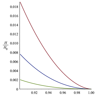
Figure 1: The evolution of $\frac{H}{H_{0}}$ versus $\theta$ for various $\epsilon_{1}=0.02,~{}0.04,~{}0.06$ (red, blue, green)

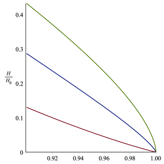
Figure 2: The evolution of $\frac{H}{H_{0}}$ versus $\theta$ for various $n_{2}=1.5,~{}2,~{}2.5$ (red, blue, green)

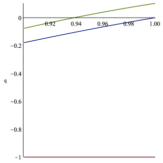
Figure 3: The evolution of $q$ versus $\theta$ for various $b=0,~{}2/3,~{}0.7$ (red, blue, green)

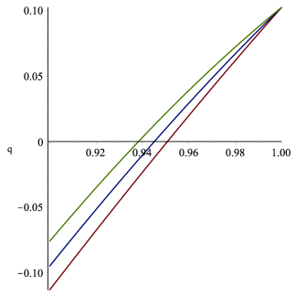
Figure 4: The evolution of $q$ versus $\theta$ for various $n_{2}=1.5,~{}2.0,~{}2.5$ (red, blue, green)

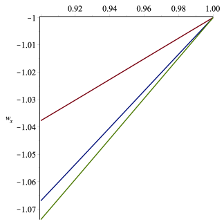
Figure 5: The evolution of $w_{x}$ versus $\theta$ for various $b=0.5,~{}2/3,~{}0.7$ (red, blue, green)

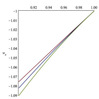
Figure 6: The evolution of $w_{x}$ versus $\theta$ for various $n_{2}=2.0,~{}4.0,~{}6.0$ (red, blue, green)

V concluding remarks

After recent efforts, especially in 2021, on relic gravitational waves from the merging of many black holes in the collapsed phase of the universe in the pre-bounce regime, cyclic cosmology came to life again. Among models that are well-adapted to cosmological data, a deformed matter bounce scenario in which the matter is deformed by a component of RVM-DE is a good candidate for study. Our hypothesis is that just as at the time of bounce, where the energy density of radiation causes a critical density to reach the LQC energy level, in the turnaround phase, The dark energy that grows up to the critical energy, provides LQC energy condition. To prove this claim, we need a model of dark energy whose energy density can grow in the phantom phase to reach the critical energy and finally remains at the phantom wall in the rapid contraction phase of the universe. In this article, we seek to prove the capability of the RVM dark energy model in turnaround the universe from expanding to contracting. Following a previous study in which we found a successful case of the RVM-CDM model in which the running of the spectral index can accept a negative value, I was interested in one of the successful cases of the interacting model of the RVM-CDM, $\rho_{x}=n_{0}+n_{2}H^{2}+n_{4}H^{4}$. The turnaround conditions at the end of expansion before the occurrence of a sudden big rip in a finite future were investigated. At the turnaround point, the Hubble parameter must vanish, the EoS parameter must be equal to $w_{x}=-1$ for all choosing parameters, and the deceleration parameter must change from a negative to positive value near the turning point. After analyzing the Hubble parameter $H$, a new restriction between parameters of model was obtained. Also by considering the deceleration parameter and EoS parameter, around the turnaround, we obtained a minimum value for interaction parameter $b=2/3$. Therefore non-interacting models must be ignored and can not create a successful turnaround. The universe behaves in the phantom regime, before any cyclicity and transition from an expansion to contraction at a finite time. At last the effect of each parameter in turnaround was studied and we saw that the transition time from accelerating to decelerating expansion occurs earlier for larger values of interaction parameter $b$. Also in several graphs the effect of second term of RVM energy density, including $H^{2}$, was studied in parameter $n_{2}$. Increasing $n_{2}$, will reduce the time of transition point and will increase in the rate of $H$ reduction. With this study, we showed that just as the RVM-CDM model can create a successful bounce, it can also be considered as a successful model for the future turnaround of the universe from an accelerated expansion to a contraction, in the presence of interaction.

References

- Tolman (1934) R. C. Tolman, Relativity Thermodynamics and Cosmology (Oxford, Clarendon Press, 1934).
- Caldwell et al. (2003) R. R. Caldwell, M. Kamionkowski, and N. N. Weinberg, Phys. Rev. Lett. 91, 071301 (2003), eprint astro-ph/0302506.
- Nojiri et al. (2012) S. Nojiri, S. D. Odintsov, and D. Saez-Gomez, AIP Conf. Proc. 1458, 207 (2012), eprint 1108.0767.
- Penrose (2011) R. Penrose, Cycles of time: an extraordinary new view of the universe (Bodley Head (UK), Knopf (US), 2011).
- Penrose (2006) R. Penrose, Conf. Proc. C 060626, 2759 (2006).
- Penrose (2012) R. Penrose, AIP Conf. Proc. 1446, 233 (2012).
- Gurzadyan and Penrose (2011) V. G. Gurzadyan and R. Penrose (2011), eprint 1104.5675.
- Gurzadyan and Penrose (2013) V. G. Gurzadyan and R. Penrose, Eur. Phys. J. Plus 128, 22 (2013), eprint 1302.5162.
- Gurzadyan and Penrose (2016) V. G. Gurzadyan and R. Penrose, Eur. Phys. J. Plus 131, 11 (2016), eprint 1512.00554.
- Penrose (2017) R. Penrose (2017), eprint 1707.04169.
- An et al. (2020) D. An, K. A. Meissner, P. Nurowski, and R. Penrose, Mon. Not. Roy. Astron. Soc. 495, 3403 (2020), eprint 1808.01740.
- Steinhardt and Turok (2002) P. J. Steinhardt and N. Turok, Phys. Rev. D 65, 126003 (2002), eprint hep-th/0111098.
- Steinhardt et al. (2002) P. J. Steinhardt, N. Turok, and N. Turok, Science 296, 1436 (2002), eprint hep-th/0111030.
- Steinhardt and Turok (2003) P. J. Steinhardt and N. Turok, Nucl. Phys. B Proc. Suppl. 124, 38 (2003), eprint astro-ph/0204479.
- Boyle et al. (2004) L. A. Boyle, P. J. Steinhardt, and N. Turok, Phys. Rev. D 69, 127302 (2004), eprint hep-th/0307170.
- Khoury et al. (2004) J. Khoury, P. J. Steinhardt, and N. Turok, Phys. Rev. Lett. 92, 031302 (2004), eprint hep-th/0307132.
- Steinhardt and Turok (2005) P. J. Steinhardt and N. Turok, New Astron. Rev. 49, 43 (2005), eprint astro-ph/0404480.
- Lehners and Steinhardt (2008) J.-L. Lehners and P. J. Steinhardt, Phys. Rev. D 78, 023506 (2008), [Erratum: Phys.Rev.D 79, 129902 (2009)], eprint 0804.1293.
- Lehners and Steinhardt (2013) J.-L. Lehners and P. J. Steinhardt, Phys. Rev. D 87, 123533 (2013), eprint 1304.3122.
- Ijjas and Steinhardt (2016) A. Ijjas and P. J. Steinhardt, Phys. Rev. Lett. 117, 121304 (2016), eprint 1606.08880.
- Ijjas and Steinhardt (2017) A. Ijjas and P. J. Steinhardt, Phys. Lett. B 764, 289 (2017), eprint 1609.01253.
- Ijjas and Steinhardt (2018) A. Ijjas and P. J. Steinhardt, Class. Quant. Grav. 35, 135004 (2018), eprint 1803.01961.
- Ijjas and Steinhardt (2022) A. Ijjas and P. J. Steinhardt, Phys. Lett. B 824, 136823 (2022), eprint 2108.07101.
- Ijjas and Steinhardt (2019) A. Ijjas and P. J. Steinhardt, Phys. Lett. B 795, 666 (2019), eprint 1904.08022.
- Baum and Frampton (2007) L. Baum and P. H. Frampton, Phys. Rev. Lett. 98, 071301 (2007), eprint hep-th/0610213.
- Frampton (2006) P. H. Frampton, in 2006 International Workshop on the Origin of Mass and Strong Coupling Gauge Theories (SCGT 06) (2006), pp. 331–337, eprint astro-ph/0612243.
- Frampton (2007) P. H. Frampton, Mod. Phys. Lett. A 22, 2587 (2007), eprint 0705.2730.
- Aref’eva et al. (2009) I. Aref’eva, P. H. Frampton, and S. Matsuzaki, Proc. Steklov Inst. Math. 265, 59 (2009), eprint 0802.1294.
- Frampton and Ludwick (2013) P. H. Frampton and K. J. Ludwick, Mod. Phys. Lett. A 28, 1350125 (2013), eprint 1304.5221.
- Corianò and Frampton (2019) C. Corianò and P. H. Frampton, Mod. Phys. Lett. A 35, 1950355 (2019), eprint 1906.10090.
- Singh (2009) P. Singh, Class. Quant. Grav. 26, 125005 (2009), eprint 0901.2750.
- Ashtekar and Singh (2011) A. Ashtekar and P. Singh, Class. Quant. Grav. 28, 213001 (2011), eprint 1108.0893.
- Wilson-Ewing (2013) E. Wilson-Ewing, JCAP 1303, 026 (2013), eprint 1211.6269.
- Gorkavyi (2022) N. Gorkavyi, New Astron. 91, 101698 (2022), eprint 2110.10218.
- Gasperini and Veneziano (1993) M. Gasperini and G. Veneziano, Astropart. Phys. 1, 317 (1993), eprint hep-th/9211021.
- Khoury et al. (2001) J. Khoury, B. A. Ovrut, P. J. Steinhardt, and N. Turok, Phys. Rev. D64, 123522 (2001), eprint hep-th/0103239.
- Brandenberger and Vafa (1989) R. H. Brandenberger and C. Vafa, Nucl. Phys. B316, 391 (1989).
- Nayeri et al. (2006) A. Nayeri, R. H. Brandenberger, and C. Vafa, Phys. Rev. Lett. 97, 021302 (2006), eprint hep-th/0511140.
- Finelli and Brandenberger (2002) F. Finelli and R. Brandenberger, Phys. Rev. D65, 103522 (2002), eprint hep-th/0112249.
- Lin et al. (2011) C. Lin, R. H. Brandenberger, and L. Perreault Levasseur, JCAP 1104, 019 (2011), eprint 1007.2654.
- Cai et al. (2013) Y.-F. Cai, E. McDonough, F. Duplessis, and R. H. Brandenberger, JCAP 1310, 024 (2013), eprint 1305.5259.
- Lehners and Wilson-Ewing (2015) J.-L. Lehners and E. Wilson-Ewing, JCAP 10, 038 (2015), eprint 1507.08112.
- Cai et al. (2016a) Y.-F. Cai, F. Duplessis, D. A. Easson, and D.-G. Wang, Phys. Rev. D93, 043546 (2016a), eprint 1512.08979.
- Cai et al. (2016b) Y.-F. Cai, A. Marciano, D.-G. Wang, and E. Wilson-Ewing, Universe 3, 1 (2016b), eprint 1610.00938.
- Ade et al. (2016a) P. A. R. Ade et al. (Planck), Astron. Astrophys. 594, A20 (2016a), eprint 1502.02114.
- Ade et al. (2016b) P. A. R. Ade et al. (Planck), Astron. Astrophys. 594, A13 (2016b), eprint 1502.01589.
- Ade et al. (2015) P. A. R. Ade et al. (BICEP2, Planck), Phys. Rev. Lett. 114, 101301 (2015), eprint 1502.00612.
- Ade et al. (2018) P. A. R. Ade et al. (BICEP2, Keck Array), Phys. Rev. Lett. 121, 221301 (2018), eprint 1810.05216.
- Cai and Wilson-Ewing (2014) Y.-F. Cai and E. Wilson-Ewing, JCAP 1403, 026 (2014), eprint 1402.3009.
- Cai and Wilson-Ewing (2015) Y.-F. Cai and E. Wilson-Ewing, JCAP 1503, 006 (2015), eprint 1412.2914.
- Arab and Khodam-Mohammadi (2018) M. Arab and A. Khodam-Mohammadi, Eur. Phys. J. C 78, 243 (2018), eprint 1707.06464.
- Arab and Khorasani (2021) M. Arab and M. Khorasani (2021), eprint 2107.08331.
- Zhang et al. (2007) J.-f. Zhang, X. Zhang, and H.-y. Liu, Eur. Phys. J. C 52, 693 (2007), eprint 0708.3121.
- Sheykhi et al. (2018) A. Sheykhi, M. Tavayef, and H. Moradpour, Can. J. Phys. 96, 1034 (2018), eprint 1706.04433.
- Ashtekar et al. (2006) A. Ashtekar, T. Pawlowski, and P. Singh, Phys. Rev. D74, 084003 (2006), eprint gr-qc/0607039.
- Perico et al. (2013) E. L. D. Perico, J. A. S. Lima, S. Basilakos, and J. Sola, Phys. Rev. D 88, 063531 (2013), eprint 1306.0591.
- Shapiro and Sola (2000) I. L. Shapiro and J. Sola, Phys. Lett. B 475, 236 (2000), eprint hep-ph/9910462.
- Shapiro and Sola (2002) I. L. Shapiro and J. Sola, JHEP 02, 006 (2002), eprint hep-th/0012227.
- Babic et al. (2005) A. Babic, B. Guberina, R. Horvat, and H. Stefancic, Phys. Rev. D 71, 124041 (2005), eprint astro-ph/0407572.
- Shapiro et al. (2003) I. L. Shapiro, J. Sola, C. Espana-Bonet, and P. Ruiz-Lapuente, Phys. Lett. B 574, 149 (2003), eprint astro-ph/0303306.
- Espana-Bonet et al. (2004) C. Espana-Bonet, P. Ruiz-Lapuente, I. L. Shapiro, and J. Sola, JCAP 02, 006 (2004), eprint hep-ph/0311171.
- Shapiro and Sola (2004) I. L. Shapiro and J. Sola, Nucl. Phys. B Proc. Suppl. 127, 71 (2004), eprint hep-ph/0305279.
- Sola (2008) J. Sola, J. Phys. A 41, 164066 (2008), eprint 0710.4151.
- Shapiro and Sola (2009) I. L. Shapiro and J. Sola, Phys. Lett. B 682, 105 (2009), eprint 0910.4925.
- Basilakos et al. (2009) S. Basilakos, M. Plionis, and J. Solà, Phys. Rev. D 80, 083511 (2009), eprint 0907.4555.
- Grande et al. (2011) J. Grande, J. Sola, S. Basilakos, and M. Plionis, JCAP 08, 007 (2011), eprint 1103.4632.
- Basilakos et al. (2012) S. Basilakos, D. Polarski, and J. Sola, Phys. Rev. D 86, 043010 (2012), eprint 1204.4806.
- Lima et al. (2013) J. A. S. Lima, S. Basilakos, and J. Sola, Mon. Not. Roy. Astron. Soc. 431, 923 (2013), eprint 1209.2802.
- Sola (2013) J. Sola, J. Phys. Conf. Ser. 453, 012015 (2013), eprint 1306.1527.
- Solà and Gómez-Valent (2015) J. Solà and A. Gómez-Valent, Int. J. Mod. Phys. D24, 1541003 (2015), eprint 1501.03832.
- Solà et al. (2017) J. Solà, A. Gómez-Valent, and J. de Cruz Pérez, Astrophys. J. 836, 43 (2017), eprint 1602.02103.
- Wilson-Ewing (2012) E. Wilson-Ewing, Class. Quant. Grav. 29, 085005 (2012), eprint 1108.6265.
- Cailleteau et al. (2012) T. Cailleteau, A. Barrau, J. Grain, and F. Vidotto, Phys. Rev. D 86, 087301 (2012), eprint 1206.6736.