Impact of Charge on Gravastars in $f(\mathfrak{R},\mathcal{T}^{2})$ Gravity

Abstract

This paper studies the influence of charge on a compact stellar structure also regarded as vacuum condensate star in the background of $f(\mathfrak{R},\mathcal{T}^{2})$ gravity. This object is considered the alternate of black hole whose structure involves three distinct regions, i.e., interior, exterior and thin-shell. We analyze these domains of a gravastar for a particular model of this modified theory. In the inner region of a gravastar, the considered equation of state defines that energy density is equal to negative pressure which is the cause of repulsive force on the spherical shell. In the intermediate shell, pressure and energy density are equal and contain ultra-relativistic fluid. The inward-directed gravitational pull of thin-shell counterbalance the force exerted by the inner region of a gravastar allowing the formation of a singularity-free object. The Reissner-Nordstrom metric presents the outer vacuum spherical domain. Moreover, we discuss the impact of the charge on physical attributes of a gravastar such as the equation of state parameter, entropy, proper length and energy. We conclude that singularity-free solutions of charged gravastar are physically consistent in this modified theory.

Keywords: Energy-momentum squared gravity; Gravastars; Compact stellar structures.
PACS: 04.20.Jb; 98.35.Ac; 04.50.Kd.

1 Introduction

Cosmic evolution is an accumulation of substantial changes including dark energy and gravitational collapse, which has developed the interest of researchers to debate on a variety of problems of cosmology as well as gravitational physics. When the fuel in the core of a star runs out and there is not enough pressure to counteract the strong gravitational pull, the star collapses, resulting in the formation of new compact objects. The rapid expansion of the cosmos is confirmed through several astrophysical observations such as supernova type Ia and cosmic microwave background. Alternative gravitational theories support expanding behavior of the universe. These theories are considered the most favorable and remarkable techniques to discover hidden attributes of the cosmos. These approaches are constructed by adding higher order curvature invariants in the geometric part of the Einstein-Hilbert action. The $f(\mathfrak{R})$ gravity is the natural extension of general relativity (GR) which discusses some novel aspects of cosmos [1].

Many researchers have shown a keen interest in the idea of curvature and matter coupling. These modified proposals explain the rotation curves of galaxies and various cosmic eras. The conservation law does not hold in these theories, assuring the existence of an extra force on particles. These theories are assumed to be an excellent candidate to understand the dark cosmos. The minimal curvature-matter coupling was developed in [2] named as $f(\mathfrak{R},T)$ gravity, while non-minimal coupled theory is $f(\mathfrak{R},{T},{\mathfrak{R}}_{\gamma\delta}{T}^{\gamma\delta})$ gravity [3]. The presence of singularities in GR is a major problem due to their prediction in high energy regions, where GR is not viable due to quantum effects and there is no specific approach in quantum theory. Accordingly, a new modification of GR has been developed by adding the analytic function ${T}_{\gamma\delta}{T}^{\gamma\delta}=\mathcal{T}^{2}$ in the functional action of $f(\mathfrak{R})$ theory [4], dubbed as $f(\mathfrak{R},\mathcal{T}^{2})$ gravity. This modified theory is also known as energy-momentum squared gravity (EMSG) which includes squared components of the matter variables, that can be used to examine several interesting astrophysical consequences. In the early universe, this theory has a regular bounce, i.e., finite maximum energy density as well as small-scale parameter [5]. As a result, the big-bang singularity can be resolved using this non-quantum prescription.

It is worth noting that this gravity overcomes the singularity of spacetime without affecting the cosmological evolution. Board and Barrow [6] investigated exact solutions with perfect matter configuration in the presence of a specific EMSG model. Nari and Roshan [7] studied dense objects that were stable as well as physically realistic. Bahamonde et al. [8] explored different EMSG coupling models (minimal/non-minimal) and found that these models unveil mysteries of the cosmos. This theory incorporates significant work and illustrates numerous cosmic implications [9].

A hypothetical highly compact star free from a singularity is suggested as a promising substitute for the black hole, which may be developed by scrutinizing the essential concept of Bose-Einstein condensation, known as gravastar. Mazur and Motolla [10] proposed this unique model which provides the corresponding solution of the Einstein field equations, they fabricated this cold and dark object as a gravitationally vacuum star or gravastar. Several researchers are interested to study the structure of gravastar because this model is expected to resolve two major issues associated with black hole structure: the singularity formation and the information paradox. The gravastar structure comprises of three different domains, interior region, thin-shell, and exterior region. The connection between state variables in the inner domain is of the type $\varrho=-\mathcal{P}$, where $\varrho$ and $\mathcal{P}$ represent energy density and pressure, respectively. These matter configuration yields non-attractive force which is responsible to produce enough pressure to resist the collapsing phenomenon. This interior zone is guarded by a thin-shell that holds stiff fluid obeying the following relationship $\varrho=\mathcal{P}$. The inner domain experiences inward-directed force exerted by the shell, consequently hydrostatic equilibrium is maintained and a singularity-free compact object is formed. The exterior domain is completely vacuumed and satisfies the equation of state (EoS) $\varrho=0=\mathcal{P}$.

There is no observational evidence in the support of gravastar, but few indirect evidence justifies the existence of gravastar structure. Sakai et al. [11] provided the criteria to detect the gravastar by investigating their shadows. Kubo and Sakai [12] used gravitational lensing to detect gravastar by observing maximum luminosity effects. But, these effects are not found in black holes with equal mass. Moreover, using interferometric LIGO detectors, a cosmic event GW150914 observed a ringdown signal [13]-[14]. These signals are released by objects having no event horizon, thus, strongly suggesting the presence of gravastar. Recently, an image taken by the first M87 Event Horizon Telescope has been examined and found likely to gravastar [15].

Visser and Wiltshire [16] investigated the stability of gravastars in GR corresponding to specific EoS and found dynamically stable gravastar structures. Carter [17] demonstrated non-singular solutions of gravastars to examine their various characteristics. Horvat and Ilijić [18] studied the gravastar configuration by taking inner de Sitter and outer Schwarzschild black hole. There is extensive literature on gravastar solutions with different matter contents [19]-[24]. Ghosh et al. [25] analyzed higher-dimensional gravastars and results were compared with 4-dimensional analog model. The astonishing findings of gravastars inspired the research community to analyze their physical attributes in modified theories [26]-[31].

Electromagnetism plays a crucial role in the study of structure evolution and stability of collapsing celestial objects. To maintain the equilibrium state of a stellar object, a star needs an enormous amount of charge to overcome the strength of the gravitational pull. Lobo and Arellano [32] developed gravastar solutions incorporating nonlinear electrodynamics and investigated its significant structural properties. Horvat et al. [33] discussed charged gravastar and computed surface redshift, the EoS parameter as well as the speed of sound for the model under consideration. Turimov et al. [34] provided a brief study on slowly rotating gravastars by taking into account extremely magnetized perfect matter. Usmani et al. [35] used conformal motion to investigate gravastar by taking charged interior and Reissner-Nordstrom metric in the exterior. It may be noted that charged interior behaves as an electromagnetic mass model and plays a key role in the stability of gravastar structure by generating gravitational mass. Rahaman et al. [36] explored gravastar structure in 3-dimensional spacetime with the contribution of charge and investigated several viable features for such compact structures. Ghosh et al. [37] established a charged gravastar model in a higher-dimensional manifold and found that physical attributes ensure the viability of the model. Sharif and Javed [38] investigated the stability of gravastars in the framework of quintessence as well as regular black hole geometries and obtained a continuously increasing profile of physical characteristics corresponding to thickness of thin-shell.

Sharif and Waseem [39] analyzed charged gravastar structure using conformal motion in realm of $f(\mathfrak{R},T)$ gravity. Yousaf et al. [40] studied charged gravastar in the same gravity and discussed its stability. Bhatti et al. [41] explored the stability of charged gravastar in the modified gravity. Bhar and Rej [42] studied gravastar admitting conformal motion to analyze the contribution of charge on the stability of the considered model. Bhatti and his collaborators [43] also investigated gravastars in the realm of ${f(\mathcal{G})}$ gravity, where $\mathcal{G}$ defines Gauss-Bonnet invariant. They investigated different attributes of gravastar with and without electromagnetic field. Various attributes of gravastar solutions are also analyzed through the gravitational decoupling technique [44]. We have studied gravastar structure with Kuchowicz metric in the context of EMSG gravity [45] . Recently, Sharif and Saeed [46] studied charge-free gravastar accepting conformal motion in the background of $f(\mathfrak{R},\mathcal{T}^{2})$ gravity and discussed the behavior of various physical attributes. Motivated by numerous works presenting effects of charge, we are interested to analyze the influence of charge on the gravastar model in $f(\mathfrak{R},\mathcal{T}^{2})$ gravity.

This paper explores the influence of charge on the geometry of gravastar in the background of $f(\mathfrak{R},\mathcal{T}^{2})$ gravity. We analyze its structure for the specific EMSG model using three different domains and also discuss physical attributes graphically. The paper is organized in the following format. Section 2 demonstrates the basic formalism of this theory under the impact of charge. Section 3 investigates the structure of charged gravastar with relevant EoS for each region and section 4 reflects various physical features of charged gravastar including EoS parameter, entropy, proper length as well as energy. We summarize the results in the last section.

2 Energy-momentum Squared Gravity

The action of EMSG theory with the inclusion of charge is classified as [4]

$$\mathcal{I}=\frac{1}{2\kappa^{2}}\int d^{4}xf\left(\mathfrak{R},{\mathcal{T}}^{2}\right){\sqrt{-g}}+\int d^{4}x(\mathcal{L}_{m}+\mathcal{L}_{e})\sqrt{-g},$$ (1)

where $g$ exhibits determinant of the metric tensor and $\kappa^{2}=8\pi$ is the coupling constant. Moreover, $\mathcal{L}_{e}=\frac{-1}{16\pi}\mathcal{F}^{\gamma\delta}\mathcal{F}_{\gamma\delta}$ where $\mathcal{F}_{\gamma\delta}=\varphi_{\delta,\gamma}-\varphi_{\gamma,\delta}$ represents the electromagnetic field tensor and $\varphi_{\gamma}$ demonstrates the four potential. In comparison to GR, the action includes additional degrees of freedom which enhance the chances to get analytical solutions. Due to the existence of an extra force and matter-dominated era, this theory offers a platform to gain significant outcomes. The variation of the action with respect to the metric tensor provides the equations of motion

$$\mathfrak{R}_{\gamma\delta}f_{\mathfrak{R}}-\frac{1}{2}g_{\gamma\delta}f+g_{\gamma\delta}\Box f_{\mathfrak{R}}-\nabla_{\gamma}\nabla_{\delta}f_{\mathfrak{R}}=\kappa^{2}T_{\gamma\delta}-\Theta_{\gamma\delta}f_{\mathcal{T}^{2}}+\kappa^{2}\mathrm{E}_{\gamma\delta},$$ (2)

where $f\equiv f(\mathfrak{R},\mathcal{T}^{2})$, $\Box=\nabla_{\gamma}\nabla^{\gamma}$, $f_{\mathfrak{R}}=\frac{\partial f}{\partial\mathfrak{R}}$, $f_{\mathcal{T}^{2}}=\frac{\partial f}{\partial\mathcal{T}^{2}}$,

$$\Theta_{\gamma\delta}=-2\mathcal{L}_{m}\left(T_{\gamma\delta}-\frac{1}{2}g_{\gamma\delta}T\right)-4\frac{\partial^{2}\mathcal{L}_{m}}{\partial g^{\gamma\delta}\partial g^{\theta\eta}}T^{\theta\eta}-TT_{\gamma\delta}+2T_{\gamma}^{\theta}T_{\delta\theta},$$ (3)

and $\mathrm{E}_{\gamma\delta}$ is the electromagnetic energy-momentum tensor given by

$$\mathrm{E}_{\gamma\delta}=\frac{1}{4\pi}\left(\mathcal{F}^{\theta}_{\gamma}\mathcal{F}_{\delta\theta}-\frac{1}{4}g_{\gamma\delta}\mathcal{F}^{\theta\eta}\mathcal{F}_{\theta\eta}\right).$$ (4)

The covariant divergence of Eq.(2) turns out to be

$$\nabla^{\gamma}T_{\gamma\delta}=\frac{1}{2\kappa^{2}}\left[-f_{\mathcal{T}^{2}}g_{\gamma\delta}{\nabla^{\gamma}}{\mathcal{T}^{2}}+2{\nabla^{\gamma}}(f_{\mathcal{T}^{2}}{\Theta_{\gamma\delta}})+\nabla^{\gamma}\mathrm{E}_{\gamma\delta}\right].$$ (5)

Due to the coupling of matter and geometry, the conservation law is failed in this theory. The field equations of EMSG reduce to $f(\mathfrak{R})$ and GR when $f(\mathfrak{R},\mathcal{T}^{2})=f(\mathfrak{R})$ and $f(\mathfrak{R},\mathcal{T}^{2})=\mathfrak{R}$, respectively. In the investigation of different astrophysical and cosmological scenarios, the distribution of matter is crucial. To examine features of the charged gravastar, we use isotropic matter distribution

$$T_{\gamma\delta}=\left(\mathcal{P}+\varrho\right)\emph{U}_{\gamma}\emph{U}_{\delta}-g_{\gamma\delta}\mathcal{P},$$ (6)

where $\emph{U}_{\gamma}$ depicts four-velocity. The matter distribution has two possible choices of $\mathcal{L}_{m}$, either we can take it as $-\varrho$, or the other choice is $\mathcal{L}_{m}=\mathcal{P}$. For minimally coupled theories of gravity, the distribution is unaffected by the choice of matter lagrangian [47]. Here, we take $\mathcal{L}_{m}=\mathcal{P}$ and using Eqs.(3) and (6), it follows that

$$\Theta_{\gamma\delta}=-\left(3\mathcal{P}^{2}+\varrho^{2}+4\mathcal{P}\varrho\right)\emph{U}_{\gamma}\emph{U}_{\delta}.$$

Manipulating Eq.(2), we have

$$\mathbb{G}_{\gamma\delta}=\frac{1}{f_{\mathfrak{R}}}\left(T_{\gamma\delta}^{c}+\kappa^{2}T_{\gamma\delta}+\kappa^{2}\mathrm{E}_{\gamma\delta}\right)=T_{\gamma\delta}^{eff},$$ (7)

where $\mathbb{G}_{\gamma\delta}=\mathfrak{R}_{\gamma\delta}-\frac{1}{2}\mathfrak{R}g_{\gamma\delta}$ is the Einstein tensor, $T_{\gamma\delta}^{c}$ denotes the additional impact of EMSG and $T_{\gamma\delta}^{eff}$ expresses the effective stress-energy given as

$$T_{\gamma\delta}^{eff}=\frac{1}{f_{\mathfrak{R}}}\bigg{\{}\kappa^{2}T_{\gamma\delta}-g_{\gamma\delta}\Box f_{\mathfrak{R}}+\nabla_{\gamma}\nabla_{\delta}f_{\mathfrak{R}}-\Theta_{\gamma\delta}f_{\mathcal{T}^{2}}+\frac{1}{2}g_{\gamma\delta}\left(f-\mathfrak{R}f_{\mathfrak{R}}\right)\bigg{\}}.$$ (8)

The field equations become highly non-linear when derivatives of multivariate functions are involved and obtaining exact solutions is more challenging. The solution to non-linear equations is obtained by employing a particular $f(\mathfrak{R},\mathcal{T}^{2})$ linear model given as [4]

$$f(\mathfrak{R},\mathcal{T}^{2})=\mathfrak{R}+\zeta\mathcal{T}^{2},$$ (9)

where $\mathcal{T}^{2}=3\mathcal{P}^{2}+\varrho^{2}$ and $\zeta$ is an arbitrary model parameter. The inclusion of $\mathcal{T}^{2}$ in this modified gravity produces more wider form of GR than the $f(\mathfrak{R})$ and $f(\mathfrak{R},T)$ theories of gravity. The functional form (9) describes the $\Lambda$CDM model and has extensively been used to solve many cosmological issues [48]. It depicts three major epochs of the universe: radiation-dominated, matter-dominated and de Sitter-dominated, while the obtained solutions indicate rapid expansion. The corresponding field equations are

$$\mathbb{G}_{\gamma\delta}=8\pi T_{\gamma\delta}+\frac{1}{2}\zeta g_{\gamma\delta}\mathcal{T}^{2}-\zeta f_{\mathcal{T}^{2}}{\Theta_{\gamma\delta}}+8\pi\mathrm{E}_{\gamma\delta}.$$ (10)

The results of GR are retrieved for $\zeta=0$.

To study the interior region of charged gravastar, we choose static spherical spacetime as

$$(ds)^{2}_{-}=e^{\chi(r)}dt^{2}-e^{\xi(r)}dr^{2}-r^{2}d\theta^{2}-r^{2}\sin^{2}\theta d\phi^{2}.$$ (11)

The corresponding non-zero Einstein tensor components are given as

$$\mathbb{G}_{0}^{0} = \Pi(r)\left(e^{\xi}-1+{\xi^{\prime}r}\right),$$ (12)

$$\mathbb{G}_{1}^{1} = \Pi(r)\left(e^{\xi}-{\chi^{\prime}r}-1\right),$$ (13)

$$\mathbb{G}_{2}^{2} = \Pi(r)\left(\frac{2r}{4}({-{\chi^{\prime}}+\xi^{\prime}})+({\chi^{\prime}\xi^{\prime}}-2{\chi^{\prime\prime}}-{\chi^{\prime 2}})\frac{{r}^{2}}{4}\right),$$ (14)

where $\Pi(r)=e^{-\xi}r^{-2}$ and prime symbolizes radial derivative. The modified equations are obtained by inserting Eqs.(6) and (12)-(14) in (10) as

$${\xi^{\prime}r}-1+e^{\xi}=\frac{r^{2}}{e^{-\xi}}\big{[}8\pi\varrho+\frac{\zeta}{2}(3{\varrho^{2}}+9{\mathcal{P}^{2}}+8\mathcal{P}\varrho)+\frac{{q}^{2}}{{r}^{4}}\big{]},$$ (15)

$$e^{\xi}-{\chi^{\prime}r}-1=\frac{r^{2}}{e^{-\xi}}\big{[}-8\pi\mathcal{P}+\frac{\zeta}{2}({\varrho^{2}}+3{\mathcal{P}^{2}})-\frac{{q}^{2}}{{r}^{4}}\big{]},$$ (16)

$$\frac{r}{2}({\xi^{\prime}}-{\chi^{\prime}})-(2{\chi^{\prime\prime}}+{\chi^{\prime 2}}-{\chi^{\prime}\xi^{\prime}})\frac{r^{2}}{4}=\frac{r^{2}}{e^{-\xi}}\big{[}\frac{\zeta}{2}({\varrho^{2}}+3{\mathcal{P}^{2}})-8\pi\mathcal{P}+\frac{{q}^{2}}{{r}^{4}}\big{]},$$

(17)

where $q$ indicates the charge of the interior sphere defined by

$$q(r)=4\pi\int_{0}^{r}r^{2}\sigma(r)e^{\chi/2}dr,\quad E(r)=\frac{r^{-2}q(r)}{4\pi}.$$ (18)

Here, $E(r)$ and $\sigma$ represent the electric field intensity and surface charge density, respectively.

The non-conserved equation (5) provides

$$\frac{d\mathcal{P}}{dr}+\chi^{\prime}(\frac{\varrho+\mathcal{P}}{2})+\aleph^{\star}-\frac{qq^{\prime}}{4\pi r^{4}}=0,$$ (19)

where $\aleph^{\star}$ shows the significant contribution of EMSG as follows

$$\aleph^{\star}=\frac{\zeta}{2}\left(3\mathcal{P}^{2}+\varrho^{2}+4\mathcal{P}\varrho\right)\chi^{\prime}+\zeta(\varrho\varrho^{\prime}+3\mathcal{P}\mathcal{P}^{\prime}).$$

Using Eq.(15), we obtain

$$e^{-\xi}=\frac{r-2m}{r}-\frac{\zeta}{3}\Big{(}\frac{3{\varrho^{2}}+9{\mathcal{P}^{2}}+8\mathcal{P}\varrho}{2}\Big{)}r^{2}-\frac{1}{r}\int\frac{q^{2}}{{r}^{2}}dr,$$ (20)

where $m=\int 4\pi{\varrho}r^{2}dr$ is the gravitational mass and $\mathcal{H}(r)=\frac{1}{r}\int\frac{q^{2}}{{r}^{2}}dr$ depicts effect of charge. This provides a relationship between matter variables and the radial metric coefficient of the considered spacetime. The hydrostatic equilibrium equation (19) reads as follows

$$\frac{d\mathcal{P}}{dr}=\frac{-\frac{\chi^{\prime}}{2}(\varrho+\mathcal{P})-\zeta\frac{\chi^{\prime}}{2}\left(3\mathcal{P}^{2}+\varrho^{2}+4\mathcal{P}\varrho\right)-\zeta\varrho\varrho^{\prime}++\frac{qq^{\prime}}{4\pi r^{4}}}{3\mathcal{P}\zeta+1},$$

where $\chi^{\prime}$ is calculated from Eqs.(16) and (20) reads as

$$\chi^{\prime}=\frac{r\big{(}8\pi\mathcal{P}-\frac{\zeta}{2}(\varrho^{2}+3{\mathcal{P}^{2}}+\frac{q^{2}}{r^{4}})\big{)}+{\frac{1}{r}\big{(}\frac{2m}{r}+\frac{\zeta}{2}(3{\varrho^{2}}+9{\mathcal{P}^{2}}+8\mathcal{P}\varrho+\mathcal{H}(r))\big{)}\frac{r^{2}}{3}}}{1-\frac{2m}{r}-\frac{\zeta}{2}(3{\varrho^{2}}+9{\mathcal{P}^{2}}+8\mathcal{P}\varrho)-\mathcal{H}(r)}.$$

This reduces to the Tolman-Oppenheimer-Volkoff equation of GR for $\zeta=0$.

3 Structure of Charged Gravastars

In this section, we investigate charged gravastar geometry by considering three regions (inner, thin-shell and outer) satisfying particular EoS. The shell of negligible thickness covers internal domain of the gravastar lying in the range $\mathbf{R}_{2}=\mathbf{R}+\epsilon>r>\mathbf{R}=\mathbf{R}_{1}$, where negligible thickness of the shell is indicated by $\mathbf{R}_{2}-\mathbf{R}_{1}=\epsilon$. The radii of the inner as well as outer regions of charged gravastars are represented by $\mathbf{R}_{1}$ and $\mathbf{R}_{2}$, respectively. The three regions of charged gravastar geometry with specific EoS for each region is given by

• Inner region $(\mathcal{J}_{1})$ $\Rightarrow$ $\mathbf{R}_{1}\geq r>0$ with $\varrho=-\mathcal{P}$,

• Thin-shell $(\mathcal{J}_{2})$ $\Rightarrow$ $\mathbf{R}+\epsilon\geq r\geq\mathbf{R}_{1}$ with $\mathcal{P}-\varrho=0$,

• Outer region $(\mathcal{J}_{3})$ $\Rightarrow$ $r>\mathbf{R}+\epsilon$ with $\varrho=0=\mathcal{P}$.

3.1 Inner Region

The interior region of charged gravastar satisfies an EoS $(\mathcal{W}=-1=\mathcal{P}/\varrho)$ that leads the relation between matter variables as $\mathcal{P}=-\varrho$. The negative pressure is responsible for outward directed repulsive force to overcome the pull exerted by thin-shell on the core of spherical charged gravastar. This particular choice of $\mathcal{W}$ is also called dark energy EoS. Using this form of EoS in Eq.(19), we get $\varrho=\varrho_{c}$ (where $\varrho_{c}$ is constant) and hence $\mathcal{P}=-\varrho_{c}$. This relation shows that pressure and density remain same in the interior of charged gravastar. Inserting this equation in Eq.(15), we acquire the radial metric function as

$$e^{-\xi}=1-\mathcal{H}(r)-\frac{2{\varrho_{c}}{r^{2}}}{3}(4\pi+\zeta{\varrho_{c}})+\frac{C_{1}}{r},$$ (21)

where $\mathcal{H}(r)$ provides the effect of charge and $C_{1}$ denotes the constant of integration. The singularity-free solution is obtained at the center of gravastar by setting $C_{1}=0$. Thus we have

$$e^{-\xi}=1-\frac{2{\varrho_{c}}{r^{2}}}{3}(4\pi+\zeta{\varrho_{c}})-\mathcal{H}(r).$$ (22)

Using Eqs.(15) and (16), we can present the correlation of unknown metric functions as

$$e^{\chi}={C_{2}}e^{-\xi},$$ (23)

where $C_{2}$ corresponds to integration constant. The mass of inner domain is

$$M=\frac{\mathbf{R}^{3}(4\pi\varrho_{c}+\zeta{\varrho_{c}^{2}})}{3}+\int\frac{q^{2}}{r^{2}}dr.$$ (24)

3.2 The Intermediate Shell Region

The non-vacuumed shell of a charged gravastar is filled with an ultra-relativistic fluid that obeys the EoS $\mathcal{P}-\varrho=0$. In connection with cold baryonic universe, Zel’dovich introduced the idea of stiff matter configuration [49]. Several researchers have employed this type of matter distribution and obtained remarkable results [50]-[54]. For this region, finding exact solution to the field equations is difficult. However, in the limit specified for this domain, i.e., $0<e^{-\xi}\ll 1$, such solutions can be found by taking into account the EoS of this region. This demonstrates that the smooth matching of inner and outer domains yields thin-shell presenting the intermediate region of charged gravastar. By implementing this constraint, the corresponding field equations can be written as

$$\frac{de^{-\xi}}{dr} = \frac{2}{r}-\frac{2q^{2}}{r^{3}}-12{\varrho_{0}}^{2}\zeta r,$$ (25)

$$\big{(}\frac{3}{2r}+\frac{\chi^{\prime}}{4}\big{)}\frac{de^{-\xi}}{dr} = \frac{1}{{r}^{2}}-\frac{2q^{2}}{r^{4}}-12{\varrho_{0}}^{2}\zeta.$$ (26)

Integration of Eq.(25) yields

$$e^{-\xi}={C_{3}}-6{\varrho_{0}}^{2}\zeta{r}^{2}+2\ln{r}-2\int\frac{q^{2}}{r^{3}}dr,$$ (27)

where ${C_{3}}$ indicates another constant of integration. Solving Eqs.(25) and (26) to find $\chi^{\prime}$ and substituting it in Eq.(19) corresponding to stiff matter configuration

$$\mathcal{P}=\varrho=\frac{1}{e^{\chi}}\int\varpi{e^{\chi}}dr+\mathcal{S}e^{-\chi},$$ (28)

where $\varpi$ depicts the additional effect of charge and EMSG gravity and $\mathcal{S}$ is another integration constant. This relationship implies that fluid distribution at the outer layer of thin-shell domain is denser than in the inner domain of shell. The evolution of energy density is illustrated in Figure 1. It can be seen that the energy density is positive across the shell.

Figure 1: Behavior of $\varrho$ $(km^{-2})$ versus thickness of thin-shell.

3.3 Outer Region

We assume that both pressure and density are zero in this region, i.e., $\varrho=0=\mathcal{P}$. The outer region of spherical charged gravastar is vacuum and is described by the Reissner-Nordstrom metric reads as

$$(ds)^{2}_{+}=\mathfrak{P}(r)dt^{2}-r^{2}(d\theta^{2}+\sin^{2}\theta d\phi^{2})-\frac{dr^{2}}{\mathfrak{P}(r)},$$ (29)

where $\mathfrak{P}(r)=\frac{r-2\mathcal{M}}{r}+\frac{\mathcal{Q}^{2}}{{r}^{2}}$ and $\mathcal{M}$ corresponds to the whole mass of gravastar. In order to examine celestial bodies, inner and outer spacetimes must be perfectly matched. The structure of charged gravastar is mainly composed of three regions named as $\mathcal{J}_{1}$, $\mathcal{J}_{2}$ and $\mathcal{J}_{3}$, where $\mathcal{J}_{2}$ acts as a connection between $\mathcal{J}_{1}$ and $\mathcal{J}_{3}$. The smooth matching of the interior and exterior geometries is ensured by Israel matching criterion [55]. The continuity of metric coefficients is maintained but it is found that their derivatives may possess discontinuity at the hypersurface. Considering Lanczos equations, the stress-energy tensor of matter surface is computed as

$$\mathcal{S}^{\lambda}_{\beta}=\left(\delta^{\lambda}_{\beta}\mu^{\alpha}_{\alpha}-\mu^{\lambda}_{\beta}\right)\frac{1}{8\pi},\quad\lambda,\beta=0,2,3,$$ (30)

where $\lambda,\beta$ denote hypersurface coordinates and $\mu_{\lambda\beta}=\mathbb{K}^{+}_{\lambda\beta}-\mathbb{K}^{-}_{\lambda\beta}$ implies extrinsic curvature discontinuity. The extrinsic curvature corresponding to $\mathcal{J}_{1}$ and $\mathcal{J}_{3}$ is defined as

$$\mathbb{K}^{\pm}_{\lambda\beta}=-\left(\frac{\partial^{2}x^{\tau}}{\partial\Phi^{\lambda}\partial\Phi^{\beta}}+\Gamma^{\tau}_{\mu\nu}\frac{\partial x^{\mu}\partial x^{\nu}}{\partial\Phi^{\lambda}\partial\Phi^{\beta}}\right)\Upsilon^{\pm}_{\tau},$$ (31)

where $\Upsilon^{\pm}_{\tau}$ and $\Phi^{\lambda}$ represent the unit normals and intrinsic coordinates of the hypersurface, respectively.

The line element of charged static spherically symmetric geometry is given as

$$ds^{2}=\mathcal{N}(r)dt^{2}-\frac{dr^{2}}{\mathcal{N}(r)}-r^{2}d\theta^{2}-r^{2}\sin^{2}\theta d\phi^{2}.$$ (32)

The corresponding unit normals are of the form

$$\Upsilon^{\pm}_{\tau}=\pm\left|g^{\mu\nu}\frac{\partial\mathcal{N}}{\partial x^{\mu}}\frac{\partial\mathcal{N}}{\partial x^{\nu}}\right|^{-\frac{1}{2}}\frac{\partial\mathcal{N}}{\partial x^{\tau}},$$ (33)

where $\Upsilon^{\tau}\Upsilon_{\tau}=1$. For perfect fluid matter configuration, we obtain $\mathbb{S}_{\lambda\beta}=$diag$(\Omega,$ $-\Psi,-\Psi)$. Hence, the surface density turns out to be

$$\Omega=-\frac{1}{4\pi\mathbf{R}}\Big{[}\sqrt{1-\frac{2\mathcal{M}}{\mathbf{R}}+\frac{\mathcal{Q}^{2}}{\mathbf{R}^{2}}}-\sqrt{1-\frac{(4\pi+\zeta{\varrho_{c}}){2{\varrho_{c}}{\mathbf{R}^{2}}}}{3}+\mathcal{H}(r)}\Big{]}.$$ (34)

Using $\mathcal{J}_{1}$ and $\mathcal{J}_{3}$ as domains of charged gravastar, we obtain respective expression of surface pressure as

$$\Psi=\frac{1}{8\pi\mathbf{R}}\Big{[}\frac{{1-\frac{\mathcal{M}}{\mathbf{R}}}}{\sqrt{1-\frac{2\mathcal{M}}{\mathbf{R}}+\frac{\mathcal{Q}^{2}}{\mathbf{R}^{2}}}}-\frac{1-\frac{(4\pi+\zeta{\varrho_{c}}){4{\varrho_{c}}{\mathbf{R}^{2}}}}{3}+\mathcal{H}(r)+\mathcal{H^{\prime}}(r)}{\sqrt{1-\frac{(8\pi+2\zeta{\varrho_{c}}){{\varrho_{c}}{\mathbf{R}^{2}}}}{3}+\mathcal{H}(r)}}\Big{]}.$$ (35)

The mass inside gravastar is calculated through Eq.(34) as follows

$${m}_{\textit{shell}}=4\pi\mathbf{R}^{2}\Omega=\mathbf{R}\Big{[}{\sqrt{1-\frac{(4\pi+\zeta{\varrho_{c}}){2{\varrho_{c}}{\mathbf{R}^{2}}}}{3}+\mathcal{H}(r)}}-\sqrt{1-\frac{2\mathcal{M}}{\mathbf{R}}+\frac{\mathcal{Q}^{2}}{\mathbf{R}^{2}}}\Big{]}.$$ (36)

Finally, the total mass of charged gravastar is

$$\mathcal{M} = {m}_{\textit{shell}}{\sqrt{1-\frac{(4\pi+\zeta{\varrho_{c}}){2{\varrho_{c}}{\mathbf{R}^{2}}+\mathcal{H}(r)}}{3}}}+\frac{(4\pi+\zeta{\varrho_{c}}){2{\varrho_{c}}{\mathbf{R}^{3}+\mathcal{H}(r)}}}{3}$$ (37)

$$- \frac{{m}_{\textit{shell}}^{2}}{2\mathbf{R}}-\frac{\mathcal{Q}^{2}}{\mathbf{R}^{2}}.$$

4 Attributes of Charged Gravastars

This section deals with the study of characteristics of charged gravastar, i.e., the EoS parameter, entropy, proper length and thin-shell energy through graphical analysis. We have analyzed these features of thin-shell for negative as well positive values of the model parameter for three different values of charge. This discussion will show viability of the spherical charged gravastar structure in the context of EMSG.

4.1 The EoS Parameter

The EoS for shell of charged gravastars at $r=\mathbf{R}$ is

$$\mathcal{W}=\frac{\Psi}{\Omega}.$$ (38)

Replacing the values of $\Psi$ and $\Omega$ in Eq.(38), we have

$$\mathcal{W}(\mathbf{R})=\frac{\frac{1}{8\pi\mathbf{R}}\Big{[}\frac{{1-\frac{\mathcal{M}}{\mathbf{R}}}}{\sqrt{1-\frac{2\mathcal{M}}{\mathbf{R}}+\frac{\mathcal{Q}^{2}}{\mathbf{R}^{2}}}}-\frac{1-\frac{(4\pi+\zeta{\varrho_{c}}){4{\varrho_{c}}{\mathbf{R}^{2}}}}{3}+\mathcal{H}(r)+\mathcal{H^{\prime}}(r)}{\sqrt{1-\frac{(8\pi+2\zeta{\varrho_{c}}){{\varrho_{c}}{\mathbf{R}^{2}}}}{3}+\mathcal{H}(r)}}\Big{]}}{-\frac{1}{4\pi\mathbf{R}}\Big{[}\sqrt{1-\frac{2\mathcal{M}}{\mathbf{R}}+\frac{\mathcal{Q}^{2}}{\mathbf{R}^{2}}}-\sqrt{1-\frac{(4\pi+\zeta{\varrho_{c}}){2{\varrho_{c}}{\mathbf{R}^{2}}}}{3}+\mathcal{H}(r)}\Big{]}}.$$ (39)

We impose some additional constraints on $\mathcal{W}(\mathbf{R})$, i.e., $\frac{2\mathcal{M}}{\mathbf{R}}+\frac{\mathcal{Q}^{2}}{\mathbf{R}^{2}}<1$ or $2\mathcal{M}<\mathbf{R}$. The relationship between $\mathcal{M}$, $\mathcal{Q}$ and $\mathbf{R}$ is obtained as $\mathcal{Q}>\sqrt{2\mathcal{M}\mathbf{R}-\mathbf{R}^{2}}$ and $2\mathcal{M}<\mathbf{R}$. Taking positive values of surface density as well as pressure results in positive value of $\mathcal{W}$. We attain $\mathcal{W}(\mathbf{R})\approx 1$ for large values of $\mathbf{R}$. The structure of gravastar is similar to compact objects for appropriately bigger values of $\mathbf{R}$. Moreover, by inserting specific value of $\mathbf{R}$ in Eq.(35) may result $\Psi=0$, which presents dust shell.

4.2 Entropy of Thin-Shell

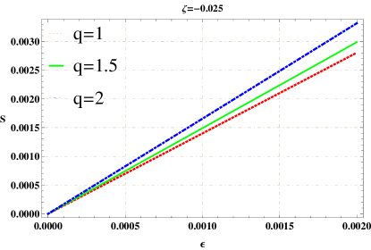
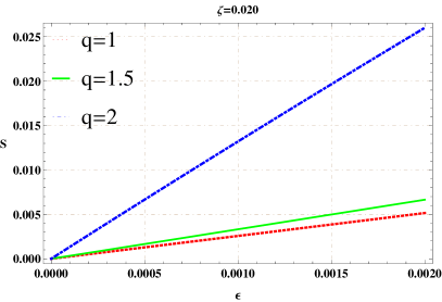
Figure 2: Entropy of the shell with thickness (km) corresponding to different values of charge.

Mazur and Mottola [10] investigated the inner region and concluded that entropy density is zero which represents reliability of condensate phase. In intermediate region, the entropy of charged gravastar is calculated as

$$S=\int^{\mathbf{R}_{2}}_{\mathbf{R}_{1}}4\sqrt{e^{\xi(r)}}\pi r^{2}\mathbb{V}(r)dr,$$ (40)

where $\mathbb{V}(r)$ shows the entropy density given as

$$\mathbb{V}(r)=\frac{\curlyvee^{2}K^{2}_{\mathcal{B}}\mathbb{T}(r)}{4\pi\hslash^{2}}=K_{\mathcal{B}}\left({\frac{\mathcal{P}}{2\pi}}\right)^{\frac{1}{2}}\frac{\curlyvee}{\hslash},$$ (41)

$\curlyvee$ is a dimensionless constant. The Planckian units are taken into account $K_{\mathcal{B}}=\hslash=1$ so that Eq.(40) becomes

$$S=\curlyvee({8\pi})^{\frac{1}{2}}\int^{\mathbf{R}_{2}}_{\mathbf{R}_{1}}\frac{({C_{3}}-6{\varrho_{0}}^{2}\zeta{r}^{2}+2\ln{r}-2\int\frac{q^{2}}{r^{3}}dr)^{\frac{-1}{2}}}{(\frac{1}{e^{\chi}}\int\varpi{e^{\chi}}dr+\mathcal{S}e^{-\chi})^{\frac{-1}{2}}}{r}^{2}dr.$$ (42)

It is too difficult to obtain an analytical solution to this equation, therefore, we solve it numerically. Figure 2 depicts the disorderness of gravastar and shows that the entropy of shell increases with the increment in thickness. The entropy is proportional to the small thickness of thin-shell. It has maximum value at the outer surface of thin-shell and zero thickness yields the value of entropy to be zero. The disorderness increases with the increasing amount of charge, thus allowing the formation of a more stable structure. The model parameter affects the entropy such that its positive value provides higher entropy as compared to its negative value.

4.3 Length of Charged Shell

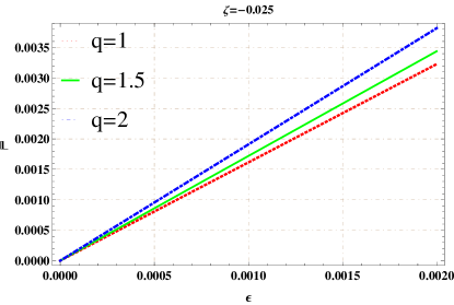
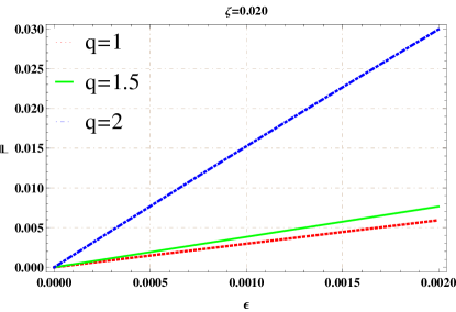
Figure 3: Proper length (km) of the charged shell against thickness (km).

The proper length of shell region is calculated from $\mathbf{R}_{1}$ to $\mathbf{R}_{2}=\mathbf{R}+\epsilon$, where $\epsilon\ll 1$ indicates negligible change. The mathematical formula of length of intermediate-shell is given by

$$\mathbb{L}=\int^{\mathbf{R}_{2}}_{\mathbf{R}_{1}}\sqrt{e^{\xi(r)}}dr=\int^{\mathbf{R}_{2}}_{\mathbf{R}_{1}}\frac{dr}{\sqrt{{C_{3}}-6{\varrho_{0}}^{2}\zeta{r}^{2}+2\ln{r}-2\int\frac{q^{2}}{r^{3}}dr}}.$$ (43)

We obtain the numerical solution of this equation and its plot is shown in Figure 3. The left panel of Figure 3 shows a continuous increment in the length of thin-shell by increasing the value of charge with $\zeta=-0.025$. However, $\zeta=0.020$ leads to the rapid increase in length of the shell for similar values of charge, presented in the right panel of Figure 3.

4.4 Thin-Shell Energy

In the core of charged gravastar, the presence of dark energy is confirmed due to negative pressure which is responsible for repulsive force. The mathematical representation of the energy is

$$\varepsilon=\int^{\mathbf{R}_{2}}_{\mathbf{R}_{1}}4\pi\varrho r^{2}dr.$$ (44)

Plugging the value of surface density in Eq.(44 yields

$$\varepsilon=\int^{\mathbf{R}_{2}}_{\mathbf{R}_{1}}4\pi{r}^{2}\left(\frac{1}{e^{\chi}}\int\varpi{e^{\chi}}dr+\mathcal{S}e^{-\chi}\right)dr.$$ (45)

This increases by enhancing its thickness as shown in Figure 4. The energy plots corresponding to both values of $\zeta$ show linear profile with the increment of charge.

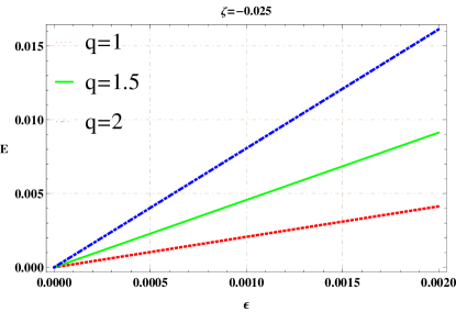
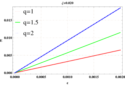
Figure 4: Plots of energy (km) of charged thin-shell versus thickness of the shell (km).

5 Conclusions

In this manuscript, we investigate the structure of charged gravastar in the background of EMSG. We have considered charged sphere in the interior with EoS $\varrho=-\mathcal{P}$ and Reissner-Nordstrom black hole in the exterior region with vacuum ($\varrho=\mathcal{P}=0$). The interior region is surrounded by a thin-shell with EoS $\varrho=\mathcal{P}$. In the intermediate shell, non-repulsive force counterbalances the pull exerted by the charged sphere and assures the formation of singularity-free compact object. It is worth mentioning that solutions corresponding to dark energy EoS show connection of charged gravastars with dark stars.

It is worth here that solutions obtained through dark energy EoS indicate that charged gravastars are linked with dark stars.

The main results are summarized as follows.

• The increasing density depicts that the shell’s external boundary is denser than the internal boundary (Figure 1).

• The real value of the EoS parameter is obtained when $\frac{2\mathcal{M}}{\mathbf{R}}+\frac{\mathcal{Q}^{2}}{\mathbf{R}^{2}}<1$. This is a necessary condition for the stable and physically viable gravastar structure.

• The entropy of charged thin-shell is proportional to its thickness, thus greater thickness means higher entropy (Figure 2). The increment of electromagnetic strength increases its entropy as well.

• The proper length of the charged thin-shell indicates increasing behavior with the thickness of the shell (Figure 3). The gravastar length goes on increasing with a higher value of the charge.

• The energy of the inner boundary is less than that of the outer domain. The thickness of the shell is shown to be linearly related to the energy of the shell (Figure 4).

It is worthwhile to mention here that the length, energy and entropy of a gravastar increase with respect to thickness of the shell as compared to the uncharged case [46]. Our analysis follows a consistent increasing trend of the physical properties in the presence of charge, presented in GR as well as other modified theories of gravity [38, 39, 42, 43]. The matching of the charged inner sphere and Reissner-Nordstrom metric produces gravitational mass which behaves as an electromagnetic mass model. The charge provides an outward-directed force, therefore, an additional repulsive force helps the gravastar from collapsing into a singularity. Thus, the presence of charge generates a more stable structure as compared to the uncharged model [46]. Furthermore, we have found that the physical attributes of gravastar have greater values in EMSG as compared to GR and other modified theories of gravity [38, 39, 42, 43]. We conclude that $f(\mathfrak{R},\mathcal{T}^{2})$ gravity successfully discusses charged gravastar model.

References

• [1] Felice, A.D. and Tsujikawa, S.R.: Living Rev. Relativ. 13(2010)3; Nojiri, S. and Odintsov, S.D.: Phys. Rep. 505(2011)59; Bamba, K. et al.: Astrophys. Space Sci. 342(2012)155.
• [2] Harko, T., Koivisto, T.S. and Lobo, F.S.N.: Mod. Phys. Lett. A 26(2011)1467.
• [3] Haghani, Z. et al.: Phys. Rev. D 88(2013)044023.
• [4] Katirci, N. and Kavuk, M.: Eur. Phys. J. Plus 129(2014)163.
• [5] Roshan, M. and Shojai, F.: Phys. Rev. D 94(2016)044002.
• [6] Board, C.V.R. and Barrow, J.D.: Phys. Rev. D 96(2017)123517.
• [7] Nari, N. and Roshan, M.: Phys. Rev. D 98(2018)024031.
• [8] Bahamonde, S., Marciu, M. and Rudra, P.: Phys. Rev. D 100(2019)083511.
• [9] Chen, C.Y. and Chen, P.: Phys. Rev. D 101(2020)064021; Bhattacharjee, S. and Sahoo, P.K.: Eur. Phys. J. Plus 135(2020)86; Sharif, M. and Gul, M.Z.: Phys. Scr. 96(2020)025002; Int. J. Mod. Phys. A 36(2021)2150004; Chin. J. Phys. 71(2021)365; Adv. Astron. 2021(2021)6663502; Eur. Phys. J. Plus 136(2021)503; Universe 7(2021)154.
• [10] Mazur, P. and Mottola, E.: Proc. Natl. Acad. Sci. USA 101(2004)9545.
• [11] Sakai, N. et al.: Phys. Rev. D 90(2014)104013.
• [12] Kubo, T. and Sakai, N.: Phys. Rev. D 93(2016)084051.
• [13] Cardoso, V. et al.: Phys. Rev. Lett. 116(2016)171101.
• [14] Cardoso, V. et al.: Phys. Rev. Lett. 117(2016)089902.
• [15] Akiyama, K. et al.: Astrophys. J. Lett. 875(2019)1.
• [16] Visser, M. and Wiltshire, D.L.: Class. Quantum Grav. 21(2004)1135.
• [17] Carter, B.M.N.: Class. Quantum Grav. 22(2005)4551.
• [18] Horvat, D. and Ilijic, S.: Class. Quantum Grav. 24(2007)5637.
• [19] Broderick, A.E. and Narayan, R.: Class. Quantum Grav. 24(2007)659.
• [20] Chirenti, C.B.M.H. and Rezzolla, L.: Class. Quantum Grav. 24(2007)4191.
• [21] Rocha, P. et al.: J. Cosmol. Astropart. Phys. 11(2008)010.
• [22] Cardoso, V. et al.: Phys. Rev. D 77(2008)124044.
• [23] Harko, T., Kovรกcs, Z. and Lobo, F.S.N.: Class. Quantum Grav. 26(2009)215006.
• [24] Pani, P. et al.: Phys. Rev. D 80(2009)124047.
• [25] Ghosh, S. et al.: Phys. Lett. B 767(2017)380.
• [26] Das, A. et al.: Phys. Rev. D 95(2017)124011.
• [27] Shamir, F. and Ahmad, M.: Phys. Rev. D 97(2018)104031.
• [28] Sharif, M. and Waseem, Eur. Phys. J. Plus. 135(2020)930.
• [29] Bhatti, M.Z. et al.: Phys. Dark Universe 29(2020)100561.
• [30] Abbas, G. and Majeed, K.: Adv. Astron. 2020(2020)8861168.
• [31] Yousaf, Z. Bhatti, M.Z. and Asad, H.: Phys. Dark Universe 28(2020)100501.
• [32] Lobo, F. S.N. and Arellano, A. V. B.: Class. Quantum Grav. 24(2007)1069.
• [33] Horvat, D., Ilijic, S. and Marunovic, A.: Class. Quantum Grav. 26(2009)025003.
• [34] Turimov, B.V., Ahmedov, B.J. and Abdujabbarov, A.A.: Mod. Phys. Lett. A 24(2009)733.
• [35] Usmani, A.A. et. al: Phys. Lett. B 701(2011)388.
• [36] Rahaman, F. et. al.: Phys. Lett. B 717(2012)1.
• [37] Ghosh, S. et. al.: Phys. Lett. B 767(2017)380.
• [38] Sharif, M. and Javed, F.: Ann. Phys. 415(2020)168124; J. Exp. Theor. Phys. 132(2021)381; Eur. Phys. J. C 81(2021)47.
• [39] Sharif, M. and Waseem, A.: Astrophys. Space Sci. 364(2019)189.
• [40] Yousaf, Z. et. al.: Phys. Rev. D 100(2019)024062.
• [41] Bhatti, M.Z. et al.: Phys. Dark Universe 29(2020)100561.
• [42] Bhar, P. and Rej, P.: Eur. Phys. J. C. 81(2021)763.
• [43] Bhatti, M.Z. et al.: Chin. J. Phys. 73(2021)167; Mod. Phys. Lett. 36(2021)2150233.
• [44] Azmat, H. Zubair, M. and Ahmad, Z.: Ann. Phys. 439(2022)168769.
• [45] Naz, S. and Sharif, M.: Universe 8(2022)142.
• [46] Sharif, M. and Saeed, M.: Chin. J. Phys. (to appear, 2022).
• [47] Faraoni, V.: Phys. Rev. D 80(2009)124040.
• [48] Akarsu, O. et. al.: Phys. Rev. D 97(2018)024011.
• [49] Zeldovich, Y.B.: Mon. R. Astron. Soc. 160(1972)1.
• [50] Carr, B.J.: Astrophys. J. 201(1975)1.
• [51] Wesson, P.S.: J. Math. Phys. 19(1978)2283.
• [52] Madsen, M.S. et al.: Phys. Rev. D 46(1992)1399.
• [53] Braje, T.M. and Romani, R.W.: Astrophys. J. 580(2002)1043.
• [54] Linares, L.P., Malheiro, M. and Ray, S.: Int. J. Mod. Phys. D 13(2004)1355.
• [55] Israel, W.: Nuovo Cimento B 44(1966)1.