Broadband X-ray Spectroscopy and Estimation of Spin of the Galactic Black Hole Candidate GRS 1758–258

Abstract

We present the results of a broadband ($0.5-78$ keV) X-ray spectral study of the persistent Galactic black hole X-ray binary GRS 1758–258 observed simultaneously by Swift and NuSTAR. Fitting with an absorbed power-law model revealed a broad Fe line and reflection hump in the spectrum. We used different flavours of the relativistic reflection model for the spectral analysis. All models indicate the spin of the black hole in GRS 1758–258 is $>0.92$. The source was in the low hard state during the observation, with the hot electron temperature of the corona estimated to be $kT_{e}\sim 140$ keV. The black hole is found to be accreting at $\sim 1.5\%$ of the Eddington limit during the observation, assuming the black hole mass of 10 $M_{\odot}$ and distance of $8$ kpc.

1 Introduction

Black hole X-ray binaries (BHXRBs) are powered by the accretion process, where matter from the companion star get accreted on to the central black hole (BH). The gravitational energy is converted to radiation emitted over the electromagnetic spectrum in the accretion process. Depending on the X-ray activity, a BHXRB can be classified into a transient or a persistent source (Tetarenko et al., 2016). The transient source spends most of the time in a quiescent state with very low X-ray luminosity ($L_{\rm X}<10^{32}$ erg s^-1) and occasionally undergoes an outbursting phase when the X-ray luminosity increases to $L_{\rm X}>10^{35}$ erg s^-1. On the other hand, a persistent source is always found to be active in X-rays with the X-ray luminosity $L_{\rm X}\sim 10^{35-37}$ erg s^-1(e.g., Tetarenko et al., 2016).

A black hole is characterized by its mass ($M_{\rm BH}$) and spin ($a^{*}$). Estimation of the BH spin is harder compared to the estimation of BH mass. There exist various direct methods to estimate the BH mass, such as radial velocity measurement of the secondary, dips and eclipses in the light curves (e.g., Kreidberg et al., 2012; Torres et al., 2019; Jana et al., 2022). The BH mass can also be estimated from the spectral modelling and timing analysis (e.g., Kubota et al., 1998; Shaposhnikov & Titarchuk, 2007, 2009; Jana et al., 2016, 2020, 2021a; Chatterjee et al., 2016). The BH spin can be measured from X-ray spectroscopy. In this method, the spin can be estimated in two processes: the continuum fitting (CF) method (CF; e.g., Zhang et al., 1997; McClintock et al., 2006; Steiner et al., 2014), and the study of Fe line and reflection spectroscopy (e.g., Fabian et al., 1989; Miller et al., 2012; Reynolds, 2020). Both methods require measuring the inner edge of the accretion disk that extends up to the inner most stable circular orbit (ISCO). It has also been suggested that the black hole spin can affect the polarization state of X-ray emission (e.g., Schnittman & Krolik, 2010; Dovčiak et al., 2011).

In the CF method, the inner radius of the accretion disk is measured by fitting the thermal disk continuum with a general relativistic model (e.g., Gierliński et al., 2001; McClintock et al., 2006; Shafee et al., 2006). In this process, one also needs to have prior knowledge of the BH mass, distance and inclination angle. On the contrary, no knowledge of BH mass or distance is required to measure the spin in reflection spectroscopy. In this method, the reflection of the coronal emission at the inner disk is studied. The essential features of the reflection spectra are Fe fluorescent emission between $6.4-6.97$ keV and a reflection hump around $15-40$ keV. The accretion disk is optically thick and geometrically thin and extends up to the ISCO (Shakura & Sunyaev, 1973). Due to the relativistic effect (Doppler shifts and gravitational redshift), the line profile of the Fe line originating from the inner accretion disk is blurred. As the ISCO depends on the spin, the study of the blurred spectra allows us to estimate the spin of the BH (Bardeen et al., 1972; Novikov & Thorne, 1973).

The spin of black hole has been estimated using either CF method or reflection spectroscopy, or both. The CF method has been used to estimate spin for LMC X–1 (Mudambi et al., 2020), LMC X–3 (Bhuvana et al., 2021), MAXI J1820+070 (Zhao et al., 2021). The reflection spectroscopy is used to estimate spin for several BHs, e.g., MAXI J1535–571 (Miller et al., 2018), XTE J1908–094 (Draghis et al., 2021), Cygnus X–1 (Tomsick et al., 2018), MAXI J1631–479 (Xu et al., 2020), GX 339–4 (García et al., 2019). Both reflection spectroscopy and CF have been used to measure the spin in a few BHs, e.g., GRS 1716–249 (Tao et al., 2019), LMC X–3 (Jana et al., 2021b), GX 339–4 (Parker et al., 2016). The majority of the BHs are found to have prograde spin, i.e., the accretion flow rotates in the same direction as the BH . Only a few BHs are found to have a retrograde spin, e.g., MAXI J1659–152 (Rout et al., 2020), Swift J1910.2-0546 (Reis et al., 2013), GS 1124–683 (Morningstar et al., 2014). Nonetheless, the spin of the BH has been observed to have a wide range. Although, the spin has been measured for a substantial number of BHs, the spin of many BH remains unknown.

GRS 1758–258 is a black hole X-ray binary located in the close vicinity of the Galactic centre. GRS 1758–258 was discovered by GRANAT/SIGMA in 1990 (Syunyaev et al., 1991). It is one of the few persistent BHXRBs in our galaxy. The source has been observed in multi-wavelengths over the years (e.g., Rodriguez et al., 1992; Mereghetti et al., 1994, 1997; Smith et al., 2001; Keck et al., 2001; Pottschmidt et al., 2006; Lin et al., 2000; Luque-Escamilla et al., 2014). It is considered to be a black hole based on its spectral and timing properties (Sidoli & Mereghetti, 2002). GRS 1758–258 is predominately found to be in the low hard state (LHS; Soria et al., 2011). From the RXTE monitoring, Smith et al. (2002) reported a state transition to the soft state in 2001 with the $3-25$ keV flux decreased by over an order of magnitude. GRS 1758–258 also shows two extended radio lobes, which makes the system a microquasar (Rodriguez et al., 1992). For a long time, the companion star was not identified due to the dense stellar population in the field. Recently, the spectroscopic study suggested that the companion is likely an A-type main-sequence star (Martí et al., 2016). The orbital period of GRS 1758–258 is reported to be $18.45\pm 0.10$ days (Smith et al., 2002).

GRS 1758–258 is the least studied source among three persistent Galactic black hole binaries. The mass and spin of the black hole in GRS 1758–258 are not known yet. In this paper, we aim to estimate the spin of the BH in GRS 1758–258 from the broadband X-ray spectroscopy. The paper is organized in the following way. We present the observation and data reduction technique in §2. In §3, we present the analysis and result. Finally, we discuss our findings in §4.

Table 1: Log of Observations of GRS 1758–258

Instrument	Date (UT)	Obs ID	Exposure (ks)	Count s-1
NuSTAR	2018-09-28	30401030002	42	$17.39\pm 0.02$
Swift/XRT	2018-09-28	00088767001	1.7	$7.88\pm 0.07$

2 Observations and Data Reduction

NuSTAR observed GRS 1758–258  on September 28, 2018 for a total exposure of 42 ks (see Table 1). NuSTAR is a hard X-ray focusing telescope, consisting of two identical modules: FPMA and FPMB (Harrison et al., 2013). The raw data were reprocessed with the NuSTAR Data Analysis Software (NuSTARDAS, version 1.4.1). Cleaned event files were generated and calibrated by using the standard filtering criteria in the nupipeline task and the latest calibration data files available in the NuSTAR calibration database (CALDB) . The source and background products were extracted by considering circular regions with radii 60 arcsec and 90 arcsec, at the source co-ordinate and away from the source, respectively. The spectra and light curves were extracted using the nuproduct task. We re-binned the spectra with 30 counts per bin by using the grppha task.

Swift/XRT observed GRS 1758–258  simultaneously with NuSTAR for an exposure of 1.7 ks in window-timing (WT) mode. The XRT spectrum did not suffer from photon pile-up. In general, the pile-up occurs if the count rate is over 100 counts s^-1 in the WT mode (Romano et al., 2006). The $0.5-10$ keV spectrum was generated using the standard online tools provided by the UK Swift Science Data Centre (Evans et al., 2009). For the present study, we used simultaneous observations of Swift/XRT and NuSTAR in the $0.5-78$ keV energy range.

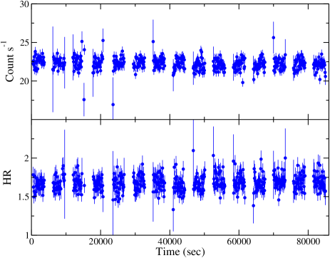
Figure 1: Top panel: $3-78$ keV light curve of GRS 1758–258  from the NuSTAR observation. The light curve is binned at 100s. Bottom panel: Variation of the hardness ratio (HR). The HR is defined as the ratio of count rates in the $6-30$ keV range to the $3-6$ keV range.

3 Analysis and Result

Figure 1 shows the $3-78$ keV light curve of GRS 1758–258  from the NuSTAR observation in the top panel. In the bottom panel of Figure 1, the variation of the hardness ratio (HR) is shown. We define the HR as the ratio of the count rate in the $6-30$ keV to the $3-6$ keV energy ranges. We did not observe any variation in the count rate or HR during the observation period. Hence, we carried out the spectral analysis using the time averaged spectrum obtained from the observation. The spectral analysis was carried out in HEASEARC’s spectral analysis package XSPEC version 12.8.2 (Arnaud, 1996). For the analysis, we used tbabs model for the interstellar absorption with the wilms abundance (Wilms et al., 2000) and the cross-section that of Verner et al. (1996).

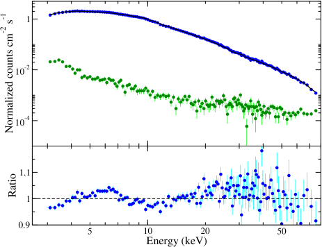
Figure 2: Top panel : cutoff model fitted NuSTAR spectrum in the $3-78$ keV energy range. The blue and green points represent the source and background count, respectively. Bottom panel : the residual in terms of data/model ratio.

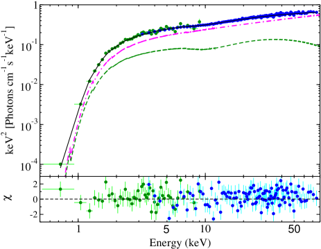
Figure 3: Top: RelxillLp model fitted $0.5-78$ keV XRT+NuSTAR unfolded spectrum. The dot-dashed magenta and dashed green lines represent the primary and reprocessed emission components, respectively.

Bottom: Corresponding residual in terms of data-model/error. The green and blue points represent the XRT and NuSTAR data, respectively.

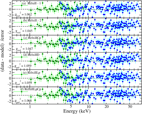
Figure 4: Residuals in terms of (data-model)/error obtained from the spectral analysis with (a) Relxill-1, (b) Relxill-2, (c) RelxillCp, (d) RelxillD, (e) RelxillLp and (f) RelxillLpCp models. The green and blue points represent the XRT and NuSTAR data, respectively. Corresponding reduced-$\chi^{2}$ is quoted in the inset of each panel.

Generally, X-ray spectra of a BHXRBs can be approximated by a multi-colour disk blackbody (MCD) and power-law components. Additionally, reprocessed emission may be observed : a Fe K$\alpha$ line at $\sim 6.4$ keV and a reflection hump at $\sim 15-40$ keV. We started our spectral analysis with the Swift/XRT+NuSTAR data in the $0.5-78$ keV energy range. The MCD component may not be present in the LHS. Thus, we attempted to fit the data with the absorbed power-law model with an exponential high energy cutoff. This model did not give us an acceptable fit with clear signatures of Fe K line, and a reflection hump in the $5-8$ keV and $15-40$ keV energy ranges, respectively. Figure 2 shows the $3-78$ keV NuSTAR spectrum in the top panel. For clarity, we only show the NuSTAR spectrum. The bottom panel of Figure 2 shows the residuals in terms of data/model ratio. We added a Gaussian line to incorporate Fe K-line in the $5-8$ keV energy range to improve the fit. Although, the fit improved with $\Delta\chi^{2}=91$ for 3 degrees of freedom (dof), it was still unacceptable as the reflection hump was clearly visible in the residuals at energies above $\sim 10$ keV.

To probe the reprocessed emission, we employed the relativistic reflection model Relxill (García et al., 2013, 2014; Dauser et al., 2014, 2016) for further spectral analysis. We applied different flavours of the Relxill model with different assumptions to the $0.5-78$ keV XRT+NuSTAR spectra. We used different Relxill family of models, namely, Relxill, RelxillCp, RelxillD, RelxillLp and RelxillLpCp for the spectral analysis. Figure 3 shows the RelxillLp model fitted XRT+NuSTAR spectrum in the $0.5-78$ keV energy range in the top panel. The dot-dashed magenta and dashed green lines represent the primary emission and reprocessed emission, respectively. Corresponding residuals in terms of data/model ratio are shown in the bottom panel. Figure 4 shows the residuals obtained from the different models in the different panels. The green and blue points represent the XRT and NuSTAR data, respectively. In the inset of each panel, the value of corresponding reduced-$\chi^{2}$ is mentioned.

3.1 Relxill

Relxill model uses a cutoff power-law as an incident primary emission. In this model, the reflection strength is measured in terms of reflection fraction ($R_{\rm refl}$) which is defined as the ratio of reflected emission to the direct emission to the observer. A broken power-law emission profile is assumed in Relxill model with $E(r)\sim R^{-q_{\rm in}}$ for $r>R_{\rm br}$ and $E(r)\sim R^{-q_{\rm out}}$ for $r<R_{\rm br}$, where E(r), $q_{\rm in}$, $q_{\rm out}$ and $R_{\rm br}$ are emissivity, inner emissivity index, outer emissivity index and break radius, respectively.

We used Relxill model in two assumptions: first by keeping the inner and outer emissivity indices fixed at the default value, i.e. $q_{\rm in}=q_{\rm out}=3$ (hereafter Relxill-1); and second, allowing the inner and outer emissivity index to vary freely (hereafter Relxill-2). During our analysis, we fixed the outer disk at $R_{\rm out}=1000~{}R_{\rm g}$. Both models gave us a good fit with $\chi^{2}$/dof = 1718/1618 and 1691/1617 for Relxill-1 and Relxill-2, respectively, although Relxill-2 gave us a better fit. Both models indicated a high spinning black hole with spin parameter, $a^{*}>0.94$. The accretion disk is found to extend almost up to the ISCO, as we obtained $R_{\rm in}=1.14^{+0.04}_{-0.03}$ $R_{\rm ISCO}$ and $1.13^{+0.02}_{-0.04}$ $R_{\rm ISCO}$ from Relxill-1 and Relxill-2, respectively. We could not constrain the cutoff energy ($E_{\rm cut}$) form these two models, as the cutoff energy pegged at the upper limit of the model at $1000$ keV. The reflection is found to be weak with $R_{\rm refl}\sim 0.23$ and $\sim 0.21$ from Relxill-1 and Relxill-2 models, respectively. With Relxill-2, we obtained a steep inner emissivity ($q_{\rm in}=6.78^{+0.05}_{-0.07}$) and a flat outer emissivity index ($q_{\rm out}=2.04^{+0.09}_{-0.06}$) with the break radius $R_{\rm br}=4.8^{+1.5}_{-0.8}$ $R_{g}$.

We also included a disk component in our spectral analysis to check if the disk is present. The thermal disk component was modelled with diskbb (Makishima et al., 1986). We obtained the inner disk temperature, $kT_{\rm in}=0.18\pm 0.12$ keV. The other spectral parameters remained the same. The addition of the disk component did not improve our fit for both Relxill-1 and Relxill-2 models. We checked if the disk component is required with FTOOLS task ftest. The ftest returned with probability=1, indicating the disk component was not required. As statistically, the disk component was not required; hence, we did not add the disk component for further analysis.

3.2 RelxillCp

For further spectral analysis, we applied the RelxillCp model for the spectral analysis. The RelxillCp has advantage over Relxill, as the RelxillCp directly estimate the coronal properties, namely, the hot electron plasma temperature ($kT_{\rm e}$). In RelxillCp, the primary incident spectrum is computed using nthcomp (Zdziarski et al., 1996; Życki et al., 1999) model, replacing cutoffpl in the Relxill model. The analysis with the RelxillCp returned with a good fit with $\chi^{2}=1691$ for 1617 dof. We obtained a similar fit with this model with the spin and inner disk radius were found to be, $a^{*}=0.97^{+0.01}_{-0.02}$ and $R_{\rm in}=1.13^{+0.03}_{-0.03}$ $R_{\rm g}$, respectively. We also obtained the temperature of the Compton corona as $kT_{e}=134^{+82}_{-29}$ keV.

3.3 High Density Model: RelxillD

Relxill and RelxillCp models consider a fixed density of the accretion disk as $n=10^{15}$ cm^-3, while RelxillD allows the density to vary. In this model, the incident primary emission is a cutoff power-law with cutoff energy fixed at 300 keV. The spectral analysis with the RelxillD model returned with a high spin $a^{*}>0.98$. We obtained a steeper emissivity with RelxillD model with $q_{\rm in}=7.09^{+0.07}_{-0.11}$, compared to the Relxill and RelxillCp models. The inclination angle of the inner disk is found to be higher with higher density, with $i=37^{+2}_{-3}$ degrees. We obtained the disk density as $n<2\times 10^{15}$ cm^-3. The detailed spectral analysis result is tabulated in Table 2.

3.4 Lamppost Geometry: RelxillLp and RelxillLpCp

In the Relxill model, no particular geometry of the corona is assumed. In the lamp post model, the corona is assumed to be a point source, located above the BH (García & Kallman, 2010; Dauser et al., 2016). RelxillLp and RelxillLpCp flavors of Relxill family of models assumed the lamp post geometry. The incident primary emission is either cutoff (RelxillLp) or nthcomp (RelxillLpCp). The height of corona ($h$) is an input parameter in this model.

We obtained a good fit with both RelxillLp and RelxillLpCp models, with the fit returned as $\chi^{2}=1715$ and $\chi^{2}=1726$ for 1619 dof, respectively. The coronal height ($h$) is obtained to be $h=3.4^{+1.1}_{-0.7}$ $R_{g}$ and $h=3.7^{+0.9}_{-0.6}$ $R_{g}$ from RelxillLp and RelxillLpCp models, respectively. The spin of the BH is obtained to be $a^{*}<0.92$ from the analysis with these models. The reflection is obtained to be stronger with $R_{\rm refl}\sim 0.46$, compared to the other models. Table 2 shows the detailed spectral analysis results with the RelxillLp and RelxillLpCp models.

3.5 Error Estimation

To calculate the uncertainty of the best-fitted spectral parameters, we ran Monte Carlo Markov Chain (MCMC) in XSPEC. The chains were run with eight walkers for a total of $10^{6}$ steps using the Goodman-Weare algorithm. We discarded the first 10000 steps of the chains, assuming to be in the ‘burn-in’ phase. The uncertainty is estimated with ‘error’ command at 1.6$\sigma$ confidence level. In the paper, we used the error at 1.6$\sigma$ level (90% confidence), or mentioned otherwise. Figure 5 shows the posterior distribution of the spectral parameters and errors obtained with the RelxillLp model. The errors are mentioned at 1 $\sigma$ level in Figure 5. Following models, like relxill, relxillCp or relxillD do not assume any coronal geometry, while relxillLp assumes lamp-post geometry. As the relxillLp provides a physical picture of the coronal geometry compared to other models mentioned before, we used RelxillLp model for the MCMC analysis.

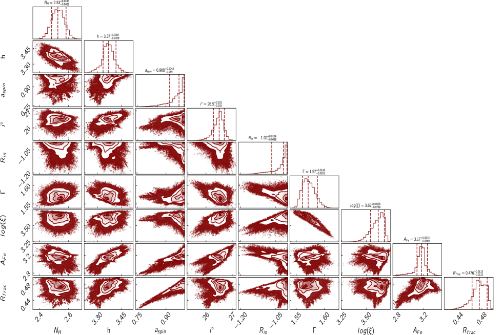
Figure 5: Posterior distribution of the spectral parameters obtained from the MCMC analysis with the RelxillLp model. Plotting was performed using corner (Foreman-Mackey, 2016) plot. Central dashed lines correspond to the peak values whereas $1\sigma$ confidence levels are represented by dashed lines on either sides.

Table 2: Spectral Analysis results

	CUTOFF	Relxill-1	Relxill-2	RelxillCp	RelxillD	RelxillLp	RelxillLpCp
$N_{\rm H}$ ($10^{22}$ cm-2)	$0.86^{+0.18}_{-0.18}$	$2.55^{+0.01}_{-0.01}$	$2.56^{+0.02}_{-0.01}$	$2.54^{+0.02}_{-0.02}$	$2.53^{+0.02}_{-0.01}$	$2.53^{+0.03}_{-0.05}$	$2.52^{+0.02}_{-0.02}$
$\Gamma$	$1.56^{+0.02}_{-0.01}$	$1.54^{+0.01}_{-0.01}$	$1.53^{+0.02}_{-0.02}$	$1.56^{+0.02}_{-0.02}$	$1.54^{+0.02}_{-0.01}$	$1.57^{+0.01}_{-0.02}$	$1.53^{+0.02}_{-0.01}$
$E_{\rm cut}$/$kT_{e}$ (keV)	$500^{+u}_{-28}$	$>946$	$>925$	$134^{+82}_{-29}$	$300^{\dagger}$	$>911$	$146^{+68}_{-32}$
$q_{\rm in}$	–	$3^{f}$	$6.78^{+0.05}_{-0.07}$	$6.51^{+0.06}_{-0.05}$	$7.09^{+0.07}_{-0.11}$	$-$	$-$
$q_{\rm out}$	–	$3^{f}$	$2.04^{+0.09}_{-0.06}$	$1.99^{+0.08}_{-0.07}$	$2.10^{+0.04}_{-0.06}$	–	–
$R_{\rm br}$/$h$ ($R_{g}$)	–	$10.8^{+2.5}_{-1.4}$	$4.8^{+1.5}_{-0.8}$	$5.3^{+1.7}_{-2.2}$	$4.5^{+1.6}_{-0.8}$	$3.4^{+0.6}_{-0.4}$	$3.7^{+0.9}_{-0.6}$
$R_{\rm in}$ ($R_{\rm ISCO}$)	–	$1.14^{+0.04}_{-0.03}$	$1.13^{+0.02}_{-0.04}$	$1.13^{+0.03}_{-0.03}$	$1.15^{+0.04}_{-0.03}$	$<1.04$	$<1.04$
$a^{*}$	–	$0.97^{+0.02}_{-0.01}$	$0.96^{+0.02}_{-0.02}$	$0.97^{+0.01}_{-0.02}$	$>0.98$	$0.97^{+0.02}_{-0.05}$	$0.95^{+0.01}_{-0.03}$
$i$ (degree)	–	$31^{+2}_{-2}$	$32^{+2}_{-4}$	$29^{+2}_{-3}$	$37^{+2}_{-3}$	$27^{+2}_{-1}$	$28^{+2}_{-2}$
$\log(n)$ (log cm-3)	–	$15^{\dagger}$	$15^{\dagger}$	$15^{\dagger}$	$<15.3$	$15^{\dagger}$	$15^{\dagger}$
$\log\xi$ (log erg cm s-1 )	–	$3.68^{+0.03}_{-0.07}$	$3.61^{+0.10}_{-0.12}$	$3.71^{+0.14}_{-0.11}$	$3.90^{+0.07}_{-0.15}$	$3.62^{+0.10}_{-0.12}$	$3.72^{+0.10}_{-0.13}$
$A_{\rm Fe}$ ($A_{\sun}$)	–	$2.75^{+0.07}_{-0.13}$	$3.16^{+0.19}_{-0.13}$	$3.16^{+0.10}_{-0.14}$	$2.99^{+0.11}_{-0.15}$	$3.17^{+0.11}_{-0.13}$	$3.28^{+0.12}_{-0.11}$
$R_{\rm refl}$	–	$0.31^{+0.02}_{-0.04}$	$0.23^{+0.02}_{-0.01}$	$0.21^{+0.04}_{-0.03}$	$0.16^{+0.02}_{-0.01}$	$0.48^{+0.03}_{-0.04}$	$0.46^{+0.03}_{-0.02}$
$N_{\rm PL}$/$N_{\rm rel}$ ($10^{-3}$ ph cm-2 s-1)	$0.12^{+0.01}_{-0.01}$	$5.02^{+0.05}_{-0.03}$	$4.75^{+0.06}_{-0.05}$	$4.68^{+0.05}_{-0.07}$	$4.61^{+0.03}_{-0.04}$	$22.7^{+0.7}_{-0.5}$	$22.7^{+0.5}_{-0.8}$
$\chi^{2}$/dof	1484/1165	1718/1618	1691/1617	1691/1617	1712/1617	1715/1619	1726/1619
$\chi^{2}_{\rm red}$	1.273	1.062	1.045	1.047	1.059	1.059	1.066
$F_{\rm 2-10~{}keV}$	$5.49^{+0.04}_{-0.03}$	$5.69^{+0.04}_{-0.05}$	$5.71^{+0.03}_{-0.04}$	$5.70^{+0.02}_{-0.03}$	$5.64^{+0.06}_{-0.05}$	$5.68^{+0.03}_{-0.04}$	$5.68^{+0.04}_{-0.05}$

^∗ indicate fixed value in the model. ^f indicate the value is fixed during the analysis.

The $F_{\rm 2-10~{}keV}$ is in unit of $10^{-10}$ ergs cm^-2 s^-1.

Errors are quoted at 1.6$\sigma$.

4 Discussion and Concluding Remarks

We studied the spectral properties of GRS 1758–258  using the data obtained by NuSTAR and Swift observatories in the energy range of $0.5-78$ keV. We used various spectral models to understand the inner accretion flow during the observation period.

Figure 5 shows the degeneracy between several parameters. The spin parameter ($a*$) is observed to be correlated with the reflection fraction ($R_{\rm refl}$) and anti-correlated with the inner disk radius ($R_{\rm in}$). These are expected as the high spin would bring the disk closer to the BH, and would make reprocessed emission strong. We also observed the photon index ($\Gamma$) is anti-correlated with the ionization parameter ($\xi$). This indicates if the photon index decreases, the ionization increases which means the hard X-rays are more effective in ionizing the disk.

During our analysis, the hydrogen column density was obtained to be $N_{\rm H}\sim 2.5\times 10^{22}$ cm^-2. However, this is higher than the previously reported $N_{\rm H}$. Soria et al. (2011) found that $N_{\rm H}\sim 1.5\times 10^{22}$ cm^-2. The discrepancy arises due to consideration of the different abundances during the spectral analysis. Soria et al. (2011) assumed the abundances to be angr (Anders & Grevesse, 1989), while we assumed wilm abundances. We checked this by assuming angr abundances during the spectral fits. Using angr abundances, the column density was obtained to be $N_{\rm H}\sim 1.5\times 10^{22}$ cm^-2.

The unabsorbed flux was obtained to be $F_{\rm 2-10~{}keV}\sim 5.7\times 10^{-10}$ erg cm^-2 s^-1  in the $2-10$ keV energy range. The bolometric flux ($F_{\rm bol}$; in the 0.1–500 keV energy band) is estimated to be $F_{\rm bol}\sim 2.6\times 10^{-9}$ erg cm^-2 s^-1. From this, we calculated the bolometric luminosity as, $L_{\rm bol}\sim 2\times 10^{37}$ erg s^-1, assuming the source distance of 8 kpc (Soria et al., 2011). Considering the mass of the BH in GRS 1758–258  as 10 $M_{\odot}$ (Soria et al., 2011), the Eddington ratio is obtained as $L/L_{\rm Edd}\sim 0.015$ or $1.5\%$ of the Eddington limit during the NuSTAR observation. GRS 1758–258 is predominately observed in a similar accretion state with the X-ray luminosity $L_{\rm X}\sim 0.01-0.03$ $L_{\rm Edd}$ (Soria et al., 2011).

The spectral analysis indicated that the source was observed in the LHS. The spectrum was found to be hard, with the photon index $\Gamma\sim 1.53-1.57$ from different spectral models. We could not estimate the cutoff energy as it was not constraint. The spectral fits with the RelxillCp gave us the temperature of the Corona as $kT_{\rm e}=134^{+82}_{-29}$ keV. Assuming lamp-post geometry, we obtained the corona temperature as $kT_{\rm e}=146^{+68}_{-32}$ keV. For completeness, we calculate the optical depth ($\tau$) of the corona using, $\tau=\sqrt{\frac{9}{4}+\frac{m_{\rm e}c^{2}}{kT_{\rm e}}\frac{3}{(\Gamma-1)(\Gamma+2)}}-\frac{3}{2}$ (Zdziarski et al., 1996). The optical depth is obtained to be $\tau=1.33^{+0.31}_{-0.54}$ for RelxillCp model. The lamp-post geometry gave $\tau=1.30^{+0.30}_{-0.37}$ which is consistent with the RelxillCp model. The observed coronal parameters are consistent with other BH in the LHS (Yan et al., 2020). The height of the corona is obtained as $h\sim 3.4$ $R_{g}$ and $h\sim 3.7$ $R_{g}$ from the lamp-post models RelxillLp and RelxillLpCp, respectively. We did not detect any signature of the accretion disk in our analysis of the $0.5-78$ keV Swift/XRT+NuSTAR spectra. We tested this by adding a disk component (diskbb in XSPEC), but the f-test rejected this. This indicated that either the disk temperature was very low or the disk normalization was low with a higher disk temperature. However, the source was observed in the LHS, where a low disk temperature is expected (e.g., Remillard & McClintock, 2006). Hence, a low temperature disk is the most probable reason for non-observation of the thermal emission.

During the spectral analysis, we started the analysis by fixing $q_{\rm in}$ and $q_{\rm out}$ at 3 (Relxill-1). In Relxill-2, RelxillCp and RelxillD models, we allowed $q_{\rm in}$ and $q_{\rm out}$ to vary freely. The outer emissivity index ($q_{\rm out}$) is found to be $\sim 2$ for all three models. We obtained a steeper inner emissivity index ($q_{\rm in}$) with all three models with $q_{\rm in}\sim 6.5-7.2$. A steep inner emissivity profile is expected as the illuminating photons will be largely beamed and focused at the inner accretion flow.

Different flavour and configuration of Relxill model indicated that the accretion disk almost extend up to the ISCO. All models predict the inner edge of the disc, $R_{\rm in}<1.2$ $R_{\rm g}$. The lamp-post models (RelxillLp and RelxillLpCp) indicated that the disk further moved towards the BH with $R_{\rm in}<1.04$ $R_{g}$. The inclination angle of the inner accretion flow is obtained to be $i\sim 26^{\circ{}}-37^{\circ{}}$ from the different model. The high density RelxillD model indicated a higher inclination with $i=37^{+2}_{-3}$ degrees while the lamp-post models indicated a lower inclination with $i\sim 28^{\circ{}}$. The reflection was found to be weak with the reflection fraction ($R_{\rm refl}$) obtained to be $R_{\rm refl}\sim 0.2$ and $\sim 0.16$ from the Relxill-2 and RelxillD models, respectively. A different geometry of the lamp-post model yields a stronger reflection with $R_{\rm refl}\sim 0.46$.

The spectral fits with the Relxill and RelxillCp models indicated the iron abundances as $A_{\rm Fe}\sim 2.7-3.2$ $A_{\sun}$. The high density RelxillD model also indicated a similar iron abundances with $A_{\rm Fe}\sim 3$ $A_{\sun}$. The RelxillLp and RelxillLpCp also indicated a similar iron abundances with $A_{\rm Fe}=3.17^{+0.11}_{-0.13}$ $A_{\sun}$ and $A_{\rm Fe}=3.28^{+0.12}_{-0.11}$ $A_{\sun}$, respectively. It is often observed that the fitting with a low density disk gives a high iron abundances (e.g., Tomsick et al., 2018). Various studies of Cygnus X–1 with the constant low density model yield the iron abundance $A_{\rm Fe}>9$ $A_{\rm Fe}$ (e.g., Walton et al., 2016; Basak et al., 2017). Tomsick et al. (2018) showed that the same spectra can be fitted with $A_{\rm Fe}=1$ $A_{\sun}$ with the density of the disk as $n\sim 4\times 10^{20}$ cm^-3. In Relxill, RelxillCp, RelxillLp and RelxillLpCp models, the disk density is considered as $n=10^{15}$ cm^-3 while the density is a free parameter in the RelxillD model. The spectral analysis of GRS 1758–258  with the RelxillD model returned the disk density as $n<2\times 10^{15}$ cm^-3. We re-analyzed the data by keeping $A_{\rm Fe}$ fixed at 1. The fit became significantly worse with $\Delta\chi^{2}>300$ for 1 dof with $n\sim 10^{18}$ cm^-3. Hence, the high density solution is not required for GRS 1758–258.

The spin of the BH in GRS 1758–258  is estimated to be very high with $a^{*}>0.93$. Relxill-1, Relxill-2 and RelxillCp indicated the spin of the BH to be $a^{*}=0.97^{+0.02}_{-0.01}$, $0.96^{+0.02}_{-0.02}$ and $0.97^{+0.01}_{-0.02}$, respectively. The RelxillD model even indicated a higher spin, with $a^{*}>0.98$. We obtained the spin of the BH as $a^{*}=0.97^{+0.02}_{-0.05}$ and $0.95^{+0.01}_{-0.03}$ from the RelxilLp and RelxillLpCp models, respectively. We also checked if a low spin solution is possible for GRS 1758–258. We fixed the spin at 0, and re-analyzed the $0.5-78$ keV XRT+NuSTAR data with all the models. All models returned with a significantly worse fit with $\Delta\chi^{2}>60$ for 1 dof. Hence, a high spin solution is preferred for GRS 1758–258.

In our analysis, we obtained a good fit from all reflection based models, with $\chi^{2}_{\rm red}\sim 1.04-1.07$. Statistically, Relxill-2 and RelxillCp returned a better fit than other variant of the model with $\Delta\chi^{2}\sim 20$. Nonetheless, our analysis shows that GRS 1758–258 hosts a high spinning BH, with $a^{*}>0.92$. In future, high resolution spetroscopy missions, such as XRISM (Tashiro et al., 2018), ATHENA (Nandra et al., 2013), AXIS (Mushotzky, 2018), Colibrí (Heyl et al., 2019; Caiazzo et al., 2019), and HEX-P (Madsen et al., 2018) are expected to constrain or reconfirm the black hole spin of GRS 1758–258 more accurately.

References

- Anders & Grevesse (1989) Anders, E., & Grevesse, N. 1989, Geochim. Cosmochim. Acta, 53, 197, doi: 10.1016/0016-7037(89)90286-X
- Arnaud (1996) Arnaud, K. A. 1996, in Astronomical Society of the Pacific Conference Series, Vol. 101, Astronomical Data Analysis Software and Systems V, ed. G. H. Jacoby & J. Barnes, 17
- Bardeen et al. (1972) Bardeen, J. M., Press, W. H., & Teukolsky, S. A. 1972, ApJ, 178, 347, doi: 10.1086/151796
- Basak et al. (2017) Basak, R., Zdziarski, A. A., Parker, M., & Islam, N. 2017, MNRAS, 472, 4220, doi: 10.1093/mnras/stx2283
- Bhuvana et al. (2021) Bhuvana, G. R., Radhika, D., Agrawal, V. K., Mandal, S., & Nandi, A. 2021, MNRAS, 501, 5457, doi: 10.1093/mnras/staa4012
- Caiazzo et al. (2019) Caiazzo, I., Belloni, T., Cackett, E., et al. 2019, Unveiling the secrets of black holes and neutron stars with high-throughput, high-energy resolution X-ray spectroscopy, Zenodo, doi: 10.5281/zenodo.3824441
- Chatterjee et al. (2016) Chatterjee, D., Debnath, D., Chakrabarti, S. K., Mondal, S., & Jana, A. 2016, ApJ, 827, 88, doi: 10.3847/0004-637X/827/1/88
- Dauser et al. (2014) Dauser, T., Garcia, J., Parker, M. L., Fabian, A. C., & Wilms, J. 2014, MNRAS, 444, L100, doi: 10.1093/mnrasl/slu125
- Dauser et al. (2016) Dauser, T., García, J., Walton, D. J., et al. 2016, A&A, 590, A76, doi: 10.1051/0004-6361/201628135
- Dovčiak et al. (2011) Dovčiak, M., Muleri, F., Goosmann, R. W., Karas, V., & Matt, G. 2011, ApJ, 731, 75, doi: 10.1088/0004-637X/731/1/75
- Draghis et al. (2021) Draghis, P. A., Miller, J. M., Zoghbi, A., et al. 2021, ApJ, 920, 88, doi: 10.3847/1538-4357/ac1270
- Evans et al. (2009) Evans, P. A., Beardmore, A. P., Page, K. L., et al. 2009, MNRAS, 397, 1177, doi: 10.1111/j.1365-2966.2009.14913.x
- Fabian et al. (1989) Fabian, A. C., Rees, M. J., Stella, L., & White, N. E. 1989, MNRAS, 238, 729, doi: 10.1093/mnras/238.3.729
- Foreman-Mackey (2016) Foreman-Mackey, D. 2016, The Journal of Open Source Software, 1, 24, doi: 10.21105/joss.00024
- García et al. (2013) García, J., Dauser, T., Reynolds, C. S., et al. 2013, ApJ, 768, 146, doi: 10.1088/0004-637X/768/2/146
- García & Kallman (2010) García, J., & Kallman, T. R. 2010, ApJ, 718, 695, doi: 10.1088/0004-637X/718/2/695
- García et al. (2014) García, J., Dauser, T., Lohfink, A., et al. 2014, ApJ, 782, 76, doi: 10.1088/0004-637X/782/2/76
- García et al. (2019) García, J. A., Tomsick, J. A., Sridhar, N., et al. 2019, ApJ, 885, 48, doi: 10.3847/1538-4357/ab384f
- Gierliński et al. (2001) Gierliński, M., Maciołek-Niedźwiecki, A., & Ebisawa, K. 2001, MNRAS, 325, 1253, doi: 10.1046/j.1365-8711.2001.04540.x
- Harrison et al. (2013) Harrison, F. A., Craig, W. W., Christensen, F. E., et al. 2013, ApJ, 770, 103, doi: 10.1088/0004-637X/770/2/103
- Heyl et al. (2019) Heyl, J., Caiazzo, I., Hoffman, K., et al. 2019, in Bulletin of the American Astronomical Society, Vol. 51, 175
- Jana et al. (2016) Jana, A., Debnath, D., Chakrabarti, S. K., Mondal, S., & Molla, A. A. 2016, ApJ, 819, 107, doi: 10.3847/0004-637X/819/2/107
- Jana et al. (2020) Jana, A., Debnath, D., Chatterjee, D., et al. 2020, ApJ, 897, 3, doi: 10.3847/1538-4357/ab9696
- Jana et al. (2021a) Jana, A., Jaisawal, G. K., Naik, S., et al. 2021a, MNRAS, 504, 4793, doi: 10.1093/mnras/stab1231
- Jana et al. (2021b) Jana, A., Naik, S., Chatterjee, D., & Jaisawal, G. K. 2021b, MNRAS, 507, 4779, doi: 10.1093/mnras/stab2448
- Jana et al. (2022) Jana, A., Naik, S., Jaisawal, G. K., et al. 2022, MNRAS, 511, 3922, doi: 10.1093/mnras/stac315
- Keck et al. (2001) Keck, J. W., Craig, W. W., Hailey, C. J., et al. 2001, ApJ, 563, 301, doi: 10.1086/323686
- Kreidberg et al. (2012) Kreidberg, L., Bailyn, C. D., Farr, W. M., & Kalogera, V. 2012, ApJ, 757, 36, doi: 10.1088/0004-637X/757/1/36
- Kubota et al. (1998) Kubota, A., Tanaka, Y., Makishima, K., et al. 1998, PASJ, 50, 667, doi: 10.1093/pasj/50.6.667
- Lin et al. (2000) Lin, D., Smith, I. A., Liang, E. P., et al. 2000, ApJ, 532, 548, doi: 10.1086/308553
- Luque-Escamilla et al. (2014) Luque-Escamilla, P. L., Martí, J., & Muñoz-Arjonilla, Á. J. 2014, ApJ, 797, L1, doi: 10.1088/2041-8205/797/1/L1
- Madsen et al. (2018) Madsen, K. K., Harrison, F., Broadway, D., et al. 2018, in Society of Photo-Optical Instrumentation Engineers (SPIE) Conference Series, Vol. 10699, Space Telescopes and Instrumentation 2018: Ultraviolet to Gamma Ray, ed. J.-W. A. den Herder, S. Nikzad, & K. Nakazawa, 106996M, doi: 10.1117/12.2314117
- Makishima et al. (1986) Makishima, K., Maejima, Y., Mitsuda, K., et al. 1986, ApJ, 308, 635, doi: 10.1086/164534
- Martí et al. (2016) Martí, J., Luque-Escamilla, P. L., & Muñoz-Arjonilla, Á. J. 2016, A&A, 596, A46, doi: 10.1051/0004-6361/201629630
- McClintock et al. (2006) McClintock, J. E., Shafee, R., Narayan, R., et al. 2006, ApJ, 652, 518, doi: 10.1086/508457
- Mereghetti et al. (1994) Mereghetti, S., Belloni, T., & Goldwurm, A. 1994, ApJ, 433, L21, doi: 10.1086/187538
- Mereghetti et al. (1997) Mereghetti, S., Cremonesi, D. I., Haardt, F., et al. 1997, ApJ, 476, 829, doi: 10.1086/303659
- Miller et al. (2012) Miller, J. M., Raymond, J., Fabian, A. C., et al. 2012, ApJ, 759, L6, doi: 10.1088/2041-8205/759/1/L6
- Miller et al. (2018) Miller, J. M., Gendreau, K., Ludlam, R. M., et al. 2018, ApJ, 860, L28, doi: 10.3847/2041-8213/aacc61
- Morningstar et al. (2014) Morningstar, W. R., Miller, J. M., Reis, R. C., & Ebisawa, K. 2014, ApJ, 784, L18, doi: 10.1088/2041-8205/784/2/L18
- Mudambi et al. (2020) Mudambi, S. P., Rao, A., Gudennavar, S. B., Misra, R., & Bubbly, S. G. 2020, MNRAS, 498, 4404, doi: 10.1093/mnras/staa2656
- Mushotzky (2018) Mushotzky, R. 2018, AXIS: A Probe Class Next Generation High Angular Resolution X-ray Imaging Satellite, arXiv, doi: 10.48550/ARXIV.1807.02122
- Nandra et al. (2013) Nandra, K., Barret, D., Barcons, X., et al. 2013, arXiv e-prints, arXiv:1306.2307. https://arxiv.org/abs/1306.2307
- Novikov & Thorne (1973) Novikov, I. D., & Thorne, K. S. 1973, in Black Holes (Les Astres Occlus), 343–450
- Parker et al. (2016) Parker, M. L., Tomsick, J. A., Kennea, J. A., et al. 2016, ApJ, 821, L6, doi: 10.3847/2041-8205/821/1/L6
- Pottschmidt et al. (2006) Pottschmidt, K., Chernyakova, M., Zdziarski, A. A., et al. 2006, A&A, 452, 285, doi: 10.1051/0004-6361:20054077
- Reis et al. (2013) Reis, R. C., Reynolds, M. T., Miller, J. M., et al. 2013, ApJ, 778, 155, doi: 10.1088/0004-637X/778/2/155
- Remillard & McClintock (2006) Remillard, R. A., & McClintock, J. E. 2006, ARA&A, 44, 49, doi: 10.1146/annurev.astro.44.051905.092532
- Reynolds (2020) Reynolds, C. S. 2020, arXiv e-prints, arXiv:2011.08948. https://arxiv.org/abs/2011.08948
- Rodriguez et al. (1992) Rodriguez, L. F., Mirabel, I. F., & Marti, J. 1992, ApJ, 401, L15, doi: 10.1086/186659
- Romano et al. (2006) Romano, P., Campana, S., Chincarini, G., et al. 2006, A&A, 456, 917, doi: 10.1051/0004-6361:20065071
- Rout et al. (2020) Rout, S. K., Vadawale, S., & Méndez, M. 2020, ApJ, 888, L30, doi: 10.3847/2041-8213/ab629e
- Schnittman & Krolik (2010) Schnittman, J. D., & Krolik, J. H. 2010, ApJ, 712, 908, doi: 10.1088/0004-637X/712/2/908
- Shafee et al. (2006) Shafee, R., McClintock, J. E., Narayan, R., et al. 2006, ApJ, 636, L113, doi: 10.1086/498938
- Shakura & Sunyaev (1973) Shakura, N. I., & Sunyaev, R. A. 1973, A&A, 500, 33
- Shaposhnikov & Titarchuk (2007) Shaposhnikov, N., & Titarchuk, L. 2007, ApJ, 663, 445, doi: 10.1086/518110
- Shaposhnikov & Titarchuk (2009) —. 2009, ApJ, 699, 453, doi: 10.1088/0004-637X/699/1/453
- Sidoli & Mereghetti (2002) Sidoli, L., & Mereghetti, S. 2002, A&A, 388, 293, doi: 10.1051/0004-6361:20020546
- Smith et al. (2001) Smith, D. M., Heindl, W. A., Markwardt, C. B., & Swank, J. H. 2001, ApJ, 554, L41, doi: 10.1086/320928
- Smith et al. (2002) Smith, D. M., Heindl, W. A., & Swank, J. H. 2002, ApJ, 578, L129, doi: 10.1086/344701
- Soria et al. (2011) Soria, R., Broderick, J. W., Hao, J., et al. 2011, MNRAS, 415, 410, doi: 10.1111/j.1365-2966.2011.18714.x
- Steiner et al. (2014) Steiner, J. F., McClintock, J. E., Orosz, J. A., et al. 2014, ApJ, 793, L29, doi: 10.1088/2041-8205/793/2/L29
- Syunyaev et al. (1991) Syunyaev, R., Gilfanov, M., Churazov, E., et al. 1991, Soviet Astronomy Letters, 17, 50
- Tao et al. (2019) Tao, L., Tomsick, J. A., Qu, J., et al. 2019, ApJ, 887, 184, doi: 10.3847/1538-4357/ab5282
- Tashiro et al. (2018) Tashiro, M., Maejima, H., Toda, K., et al. 2018, in Space Telescopes and Instrumentation 2018: Ultraviolet to Gamma Ray, ed. J.-W. A. den Herder, S. Nikzad, & K. Nakazawa, Vol. 10699, International Society for Optics and Photonics (SPIE), 520 – 531, doi: 10.1117/12.2309455
- Tetarenko et al. (2016) Tetarenko, B. E., Sivakoff, G. R., Heinke, C. O., & Gladstone, J. C. 2016, ApJS, 222, 15, doi: 10.3847/0067-0049/222/2/15
- Tomsick et al. (2018) Tomsick, J. A., Parker, M. L., García, J. A., et al. 2018, ApJ, 855, 3, doi: 10.3847/1538-4357/aaaab1
- Torres et al. (2019) Torres, M. A. P., Casares, J., Jiménez-Ibarra, F., et al. 2019, ApJ, 882, L21, doi: 10.3847/2041-8213/ab39df
- Verner et al. (1996) Verner, D. A., Ferland, G. J., Korista, K. T., & Yakovlev, D. G. 1996, ApJ, 465, 487, doi: 10.1086/177435
- Walton et al. (2016) Walton, D. J., Tomsick, J. A., Madsen, K. K., et al. 2016, ApJ, 826, 87, doi: 10.3847/0004-637X/826/1/87
- Wilms et al. (2000) Wilms, J., Allen, A., & McCray, R. 2000, ApJ, 542, 914, doi: 10.1086/317016
- Xu et al. (2020) Xu, Y., Harrison, F. A., Tomsick, J. A., et al. 2020, ApJ, 893, 30, doi: 10.3847/1538-4357/ab7dc0
- Yan et al. (2020) Yan, Z., Xie, F.-G., & Zhang, W. 2020, ApJ, 889, L18, doi: 10.3847/2041-8213/ab665e
- Zdziarski et al. (1996) Zdziarski, A. A., Johnson, W. N., & Magdziarz, P. 1996, MNRAS, 283, 193, doi: 10.1093/mnras/283.1.193
- Zhang et al. (1997) Zhang, S. N., Cui, W., & Chen, W. 1997, ApJ, 482, L155, doi: 10.1086/310705
- Zhao et al. (2021) Zhao, X., Gou, L., Dong, Y., et al. 2021, ApJ, 916, 108, doi: 10.3847/1538-4357/ac07a9
- Życki et al. (1999) Życki, P. T., Done, C., & Smith, D. A. 1999, MNRAS, 309, 561, doi: 10.1046/j.1365-8711.1999.02885.x