Abnormal subanalytic distributions
and minimal rank Sard Conjecture

Abstract

We present a description of singular horizontal curves of a totally nonholonomic analytic distribution in term of the projections of the orbits of some isotropic subanalytic singular distribution defined on the nonzero annihilator of the initial distribution in the cotangent bundle. As a by-product of our first result, we obtain, under an additional assumption on the constructed subanalytic singular distribution, a proof of the minimal rank Sard conjecture in the analytic case. It establishes that from a given point the set of points accessible through singular horizontal curves of minimal rank, which corresponds to the rank of the distribution, has Lebesgue measure zero.

1 Introduction

This article is concerned with geometrical properties of singular horizontal paths of totally nonholonomic distributions and their application to the minimal rank Sard Conjecture in the real-analytic category. Let us briefly explain the general context.

Let $M$ be a smooth (that is, $\mathcal{C}^{\infty}$) connected manifold of dimension $n\geq 3$ equipped with a totally nonholonomic distribution $\Delta$ of rank $m<n$. Horizontal paths are absolutely continuous curves which are almost everywhere tangent to $\Delta$. Among them, the so-called singular horizontal paths, which correspond to singular points of the space of horizontal paths joining their end-points, are the subject of intense research in sub-riemannian geometry (see e.g. [28, 14, 41, 37, 43, 61, 18, 7, 8]), mainly because they might be sub-Riemannian minimizers [42, 37, 44] and they can not be handled via classical techniques of calculus of variations. For example, it remains an open problem whether singular minimizing sub-riemannian geodesics are smooth (see e.g. [35, 46, 59, 31, 24, 47, 48, 4, 8, 49] for partial results and [54] for a survey by the third author), but it is simple to show that non-singular sub-riemannian geodesics are smooth [2, 45, 53]. In this context, the Sard Conjecture states that the set of points that can be attained by singular horizontal paths from a fixed point $x\in M$ has Lesbegue measure zero in $M$. The (strong version of the) Sard Conjecture has been recently proved in the real-analytic category for three dimensional manifolds [8], but the Conjecture remains open in higher dimensions: the best known-results concern Carnot groups of small rank and/or step [33, 51, 12].

A large part of this paper will be devoted to singular horizontal paths of “minimal rank”. As a matter of fact, to each singular horizontal path it is possible to attach a notion of rank $r\in\{m,\ldots,n-1\}$ which can be seen as a measure of how degenerate the path is. The minimal rank Sard conjecture is a reformulation of the Sard Conjecture, mutatis mutandis, where one only considers singular paths of minimal rank. Note that for corank $1$ distributions $\Delta$, both conjectures are equivalent. The minimal rank Sard Conjecture is equally open in dimension higher than $3$, except in the case of Carnot groups which is arguably known even if, to our knowledge, it is not stated in the literature (we provide a proof of the minimal rank Sard Conjecture for Carnot groups in $\S\S$ 2.4).

In this paper, we deal with the real-analytic category because it gives us access to techniques of subanalytic geometry and real-analytic geometry. The case of generic smooth sub-Riemannian structures, whose study is based on a different set of techniques, will be treated in a forthcoming paper [10]. Subanalytic geometry allows us to provide a precise description of singular horizontal paths (building up from the symplectic characterization due to Hsu [28]) in terms of a subanalytic isotropic distribution $\vec{\mathcal{K}}$ compatible with a subanalytic stratification of the nonzero annihilator $\Delta^{\perp}$ of the distribution in the cotangent bundle $T^{\ast}M$ (see Theorem 1.1). This approach is reminiscent to previous works by Sussmann [59] in sub-Riemannian geometry and Bove and Treves [13] in microlocal analysis. The so obtained stratification of $\Delta^{\perp}$ allows us to provide a Sard-type result for singular horizontal paths whose abnormal lifts are constrained to a single stratum of the stratification (see Theorem 1.2). Moreover, by applying symplectic methods introduced in [8] along with the notion of witness transverse section to a foliation introduced in Section 7.1, we are able to prove the minimal rank Sard Conjecture under an extra qualitative assumption over $\vec{\mathcal{K}}$ that we call splittable (see Theorem 1.5 and Definition 1.4). This qualitative property seems to be very general, for example, all line foliations are splittable (see Proposition 7.10). We are currently unaware of an analytic integrable distribution which is not splittable in an analytic Riemannian manifold, but we provide an example of an analytic foliation which is non-splittable with respect to a $\mathcal{C}^{\infty}$ metric by modifying a construction of Hirsch [27] (see Section 2.5). Before stating our result in a sharp form, we present now the precise context of this work and the main necessary definitions in detail.

Let $M$ be a smooth connected manifold of dimension $n\geq 3$ equipped with a totally nonholonomic distribution $\Delta$ of rank $m<n$, which means that for every $x\in M$ there are an open neighborhood $\mathcal{V}$ of $x$ and $m$ linearly independent smooth vector fields $X_{x}^{1},\ldots,X_{x}^{m}$ which generate $\Delta$ in $\mathcal{V}$, that is,

$$\Delta(y)=\mbox{Span}\Bigl{\{}X_{x}^{1}(y),\ldots,X_{x}^{m}(y)\Bigr{\}}\qquad\forall y\in\mathcal{V},$$

and satisfy the Hörmander condition

$$\mbox{Lie}\Bigl{\{}X_{x}^{1},\ldots,X_{x}^{m}\Bigr{\}}(y)=T_{y}M\qquad\forall y\in\mathcal{V}.$$

By Chow-Rashesvky’s theorem, any pair of points of $M$ can be connected by a horizontal path, that is, by a curve $\gamma:[0,1]\rightarrow M$ which is absolutely continuous with derivative in $L^{2}$ and satisfies

$$\dot{\gamma}(t)\in\Delta\left(\gamma(t)\right)\qquad\mbox{for a.e. }t\in[0,1].$$

We consider now the canonical symplectic form $\omega$ of $T^{*}M$ and define the nonzero annihilator of $\Delta$ as the subset of $T^{*}M$ given by

$$\Delta^{\perp}:=\Bigl{\{}{\mathfrak{a}}=(x,p)\in T^{*}M\,|\,p\neq 0\mbox{ and }p\cdot v=0,\,\forall v\in\Delta(x)\Bigr{\}}.$$ (1.1)

By construction, as a smooth vector subbundle with the zero section removed, $\Delta^{\perp}$ is a smooth submanifold of dimension $2n-m$ of $T^{*}M$ which is invariant by dilations in the fibers $\sigma_{\lambda}:T^{\ast}M\to T^{\ast}M$, with $\lambda\in\mathbb{R}^{*}$, given by $\sigma_{\lambda}(x,p)=(x,\lambda p)$ and satisfying $\sigma_{\lambda}(\Delta^{\perp})=\Delta^{\perp}$. Moreover, it is equipped with the $2$-form given by the restriction of $\omega$ denoted by

$$\omega^{\perp}:=\omega_{|\Delta^{\perp}}.$$ (1.2)

Following Hsu’s characterization [28], a singular horizontal path $\gamma:[0,1]\rightarrow M$ is an horizontal path which admits a lift $\psi:[0,1]\rightarrow\Delta^{\perp}$, called abnormal lift, satisfying

$$\dot{\psi}(t)\in\mbox{ker}\bigl{(}\omega^{\perp}_{\psi(t)}\bigr{)}\qquad\mbox{for a.e. }t\in[0,1].$$

The corank of an horizontal path is equal to the dimension of the space of abnormal lifts. It can be proved that the corank must be a number between $\{1,\ldots,n-m\}$, essentially because $\Delta^{\perp}$ is invariant by dilation and its fibers with respect to the projection to $M$ have dimension $n-m$. We say that $\gamma:[0,1]\rightarrow M$ is a minimal rank singular horizontal path if its corank is equal to $n-m$. In particular, if $\Delta$ has corank $1$, then every singular horizontal path is a minimal rank singular horizontal path.

The aforementioned results concerning singular curves are stated and proved in Section 3.2. For a more general introduction to the notions above, we refer the reader to Bellaïche’s monograph [6], or to the books by Montgomery [45], by Agrachev, Barilari and Boscain [2], or by the third author [53].

Our first result is concerned with the description of singular horizontal paths in the analytic case, that is, when both $M$ and $\Delta$ are real-analytic. Note that in this case $\Delta^{\perp}$ is an analytic submanifold in $T^{*}M$. Before stating the result, we need to introduce a few notions related to singular distributions.

We call distribution on $\Delta^{\perp}$ any mapping $\vec{\mathcal{K}}$ which assigns to a point ${\mathfrak{a}}$ in $\Delta^{\perp}\subset T^{*}M$ a vector subspace $\vec{\mathcal{K}}({\mathfrak{a}})$ of $T_{{\mathfrak{a}}}\Delta^{\perp}$ of dimension $\mbox{dim}\,\vec{\mathcal{K}}({\mathfrak{a}})$, also called rank, that may depend upon ${\mathfrak{a}}$. A curve $\psi:[0,1]\rightarrow\Delta^{\perp}$ is said to be horizontal with respect to $\vec{\mathcal{K}}$ if it is absolutely continuous with derivative in $L^{2}$ and satisfies

$$\dot{\psi}(t)\in\vec{\mathcal{K}}(\psi(t))\subset T_{\psi(t)}\Delta^{\perp}\qquad\mbox{for a.e. }t\in[0,1].$$

We say that $\vec{\mathcal{K}}$ is a subanalytic distribution if its graph in $T\Delta^{\perp}$ is subanalytic. Now, consider a subanalytic Whitney stratification of $\Delta^{\perp}$, that is a partition $\mathcal{S}=(\mathcal{S}_{\alpha})$ of $\Delta^{\perp}$,

$$\Delta^{\perp}=\bigcup_{\mathcal{S}_{\alpha}\in\mathcal{S}}\mathcal{S}_{\alpha},$$

into a locally finite union of subanalytic strata satisfying Whitney’s conditions. We say that $\mathcal{S}$ is invariant by dilation if $\sigma_{\lambda}(\mathcal{S}_{\alpha})=\mathcal{S}_{\alpha}$ for every $\alpha$ and every $\lambda\in\mathbb{R}^{\ast}$ and that $\vec{\mathcal{K}}$ is compatible with $\mathcal{S}$ if $\vec{\mathcal{K}}$ has constant rank on each $\mathcal{S}_{\alpha}$ and $\vec{\mathcal{K}}\cap T\mathcal{S}_{\alpha}$ yields an analytic subundle of $T\mathcal{S}_{\alpha}$, for all $\alpha$. In this case, we call essential domain of $\vec{\mathcal{K}}$, denoted by $\mathcal{S}_{0}$, the union of all strata of $\vec{\mathcal{K}}$ of maximal dimension, that is, of dimension $2n-m$. Finally, we say that $\vec{\mathcal{K}}$ is invariant by dilation if $d\sigma_{\lambda}(\vec{\mathcal{K}}({\mathfrak{a}}))=\vec{\mathcal{K}}(\sigma_{\lambda}({\mathfrak{a}}))$ for all ${\mathfrak{a}}$ and $\lambda$; note that $\mbox{ker}(\omega^{\perp})$ is invariant by dilation. We refer the reader to Section 3.3 for further details on the above definitions.

A subanalytic distribution $\vec{\mathcal{K}}$ compatible with a subanalytic Whitney stratification $\mathcal{S}$ is said to be integrable if for every stratum $\mathcal{S}_{\alpha}$, the restriction of $\vec{\mathcal{K}}$ to $\mathcal{S}_{\alpha}$ is closed by the Lie-bracket operation. In particular, integrable subanalytic distributions gives rise to subanalytic foliations. A subanalytic distribution $\vec{\mathcal{K}}$ on $\Delta^{\perp}$ is said to be isotropic if for every ${\mathfrak{a}}\in\Delta^{\perp}$, $\vec{\mathcal{K}}({\mathfrak{a}})$ is an isotropic space in $T_{{\mathfrak{a}}}(T^{*}M)$ with respect to $\omega$, the canonical symplectic form of $T^{*}M$, see Section 3.1 for further details.

Our first result can now be precisely stated:

Theorem 1.1 (Characterization of abnormal lifts).

Assume that both $M$ and $\Delta$ are real-analytic. Denote by $\omega$ the canonical symplectic form over $T^{\ast}M$ and by $\Delta^{\perp}\subset T^{\ast}M$ its annihilator, see (1.1). There exist an open and dense set $\mathcal{S}_{0}\subset\Delta^{\perp}$ whose complement is an analytic set, a subanalytic Whitney stratification $\mathcal{S}=(\mathcal{S}_{\alpha})$ of $\Delta^{\perp}$ invariant by dilation, where $\mathcal{S}_{0}$ is a stratum, and three subanalytic distributions

$$\vec{\mathcal{K}}\subset\vec{\mathcal{J}}\subset\vec{\mathcal{I}}\subset T\Delta^{\perp}$$

compatible with $\mathcal{S}$ and invariant by dilation satisfying the following properties:

• Specification on strata. For every stratum $\mathcal{S}_{\alpha}$ of $\mathcal{S}$, the distributions $\vec{\mathcal{K}}\subset\vec{\mathcal{J}}\subset\vec{\mathcal{I}}\subset T\Delta^{\perp}$ at a point ${\mathfrak{a}}\in\mathcal{S}_{\alpha}$ are given by

  $$\vec{\mathcal{K}}({\mathfrak{a}}):=\mbox{\em ker}\,\bigl{(}\omega^{\perp}_{{\mathfrak{a}}}\bigr{)}\cap T_{{\mathfrak{a}}}\mathcal{S}_{\alpha},\quad\vec{\mathcal{J}}({\mathfrak{a}}):=\mbox{\em Lie}\bigl{(}\vec{\mathcal{K}}_{|\mathcal{S}_{\alpha}}\bigr{)}({\mathfrak{a}}),\quad\vec{\mathcal{I}}({\mathfrak{a}}):=\mbox{\em ker}\left(\bigl{(}\omega^{\perp}_{|\mathcal{S}_{\alpha}}\bigr{)}_{{\mathfrak{a}}}\right).$$

  In particular, on each $\mathcal{S}_{\alpha}$, $\vec{\mathcal{K}},\vec{\mathcal{J}},\vec{\mathcal{I}}$ have constant rank, $\vec{\mathcal{K}}$ is isotropic, $\vec{\mathcal{J}}$ is integrable, and $\vec{\mathcal{I}}$ is both isotropic and integrable.

• Equality on the essential domain. The set $\mathcal{S}_{0}$ is the essential domain of the three distributions and

  $$\vec{\mathcal{K}}_{|\mathcal{S}_{0}}=\vec{\mathcal{J}}_{|\mathcal{S}_{0}}=\vec{\mathcal{I}}_{|\mathcal{S}_{0}}.$$

• Abnormal lifts are horizontal paths of $\vec{\mathcal{K}}$. A curve $\gamma:[0,1]\rightarrow M$ is a singular horizontal path with respect to $\Delta$ if and only if it admits a lift $\psi:[0,1]\rightarrow\Delta^{\perp}$ which is horizontal with respect to $\vec{\mathcal{K}}$.

• Ranks of $\vec{\mathcal{K}}$. The rank of $\mbox{\em ker}(\omega^{\perp}_{|\mathcal{S}_{0}})=\vec{\mathcal{K}}_{|\mathcal{S}_{0}}$ satisfies

  $$\mbox{\em dim}\,\vec{\mathcal{K}}_{|\mathcal{S}_{0}}\equiv m\,(2)\quad\mbox{and}\quad\mbox{\em dim}\,\vec{\mathcal{K}}_{|\mathcal{S}_{0}}\leq m-2,$$

  and in addition, for every stratum $\mathcal{S}_{\alpha}\neq\mathcal{S}_{0}$ of $\mathcal{S}$, the rank of $\mbox{\em ker}(\omega^{\perp}_{|\mathcal{S}_{\alpha}})$ is constant and there holds

  $$\mbox{\em dim}\,\vec{\mathcal{K}}_{|\mathcal{S}_{\alpha}}\leq m-1\quad\mbox{and}\quad\dim\mbox{\em ker}\bigl{(}\omega^{\perp}_{{\mathfrak{a}}}\bigr{)}\geq\mbox{\em dim}\,\vec{\mathcal{K}}_{|\mathcal{S}_{0}}+2\qquad\forall{\mathfrak{a}}\in\mathcal{S}_{\alpha}.$$

The proof of Theorem 1.1 is given in Section 4 and follows from techniques of subanalytic and symplectic geometry. Assertion (i) provides three distributions which in general do not coincide outside of the essential domain, we illustrate this point via an example in Section 2.3. The property given in (ii) implies that $\vec{\mathcal{K}}$ is indeed isotropic and integrable on the essential domain, this fact will play a crucial role in the proof of our result concerning the minimal rank Sard Conjecture (Theorem 1.5). Assertion (iii) is the core of Theorem 1.1, it justifies the construction of $\vec{\mathcal{K}}$ whose horizontal paths provide all abnormal lifts of $\Delta$. By combining the previous result with techniques of geometric control theory, we can demonstrate that the Sard Conjecture holds true when restricted to horizontal paths whose abnormal lifts are confined to a single stratum of the stratification given by Theorem 1.1.

Theorem 1.2 (Sard Property over strata).

Assume that both $M$ and $\Delta$ are real-analytic, and consider the notation introduced in Theorem 1.1. Let $\mathcal{S}_{\alpha}$ be a stratum equipped with a complete analytic Riemannian metric $g^{\alpha}$, for every ${\mathfrak{a}}\in\mathcal{S}_{\alpha}$ denote by $\mathcal{L}_{{\mathfrak{a}}}\subset\mathcal{S}_{\alpha}$ the leaf of the foliation generated by $\vec{\mathcal{J}}_{|\mathcal{S}_{\alpha}}$ containing ${\mathfrak{a}}$ and for every $\ell\geq 0$ by $\mathcal{L}_{{\mathfrak{a}}}^{\ell}$ the set of ${\mathfrak{a}}^{\prime}\in\mathcal{L}_{{\mathfrak{a}}}$ that can be joined to ${\mathfrak{a}}$ with a Lipschitz curve in $\mathcal{L}_{{\mathfrak{a}}}$ of length (with respect to $g^{\alpha}$) $\leq\ell$, then for every $x\in\pi(\mathcal{S}_{\alpha})$, every relatively compact subanalytic set $C\subset(\mathcal{S}_{\alpha})_{x}:=\mathcal{S}_{\alpha}\cap\Delta^{\perp}_{x}$ (with $\Delta^{\perp}_{x}=\Delta^{\perp}\cap\pi^{-1}({x})$) and every $\ell\geq 0$, the set $\mbox{\em Abn}^{C,\ell}_{\alpha}(x)\subset M$ defined by

$$\mbox{\em Abn}^{C,\ell}_{\alpha}(x):=\bigcup_{{\mathfrak{a}}\in C}\pi\left(\mathcal{L}_{{\mathfrak{a}}}^{\ell}\right)$$

is a relatively compact subanalytic set of codimension at least $1$. Moreover, if we consider a subanalytic stratification $\mathcal{T}^{\alpha}=(\mathcal{T}^{\alpha}_{\beta})$ of $(\mathcal{S}_{\alpha})_{x}$ which is invariant by dilation and compatible with $\vec{\mathcal{J}}_{|\mathcal{S}_{\alpha}}$, for every stratum $\mathcal{T}^{\alpha}_{\beta}$ the dimension of the subanalytic set

$$\mbox{\em Abn}^{C,\ell}_{\alpha,\beta}(x):=\bigcup_{{\mathfrak{a}}\in\mathcal{T}^{\alpha}_{\beta}\cap C}\pi\left(\mathcal{L}_{{\mathfrak{a}}}^{\ell}\right)$$

is bounded from above by

$$\mbox{\em dim}\,\mathcal{T}^{\alpha}_{\beta}-\mbox{\em dim}\,\vec{\mathcal{J}}_{|\mathcal{T}^{\alpha}_{\beta}}+\mbox{\em dim}\,\vec{\mathcal{J}}_{|\mathcal{S}_{\alpha}}-1$$

and if $\mathcal{S}_{\alpha}=\mathcal{S}_{0}$, then the codimension of any subanalytic set $\mbox{\em Abn}^{C,\ell}_{0,\beta}(x)$ is at least $3$. In particular, for every $x\in\pi(\mathcal{S}_{\alpha})$, the set

$$\mbox{\em Abn}_{\alpha}(x):=\bigcup_{{\mathfrak{a}}\in(\mathcal{S}_{\alpha})_{x}}\pi\left(\mathcal{L}_{{\mathfrak{a}}}\right)$$

has Lebesgue measure zero in $M$.

The proof of Theorem 1.2 is given in Section 5. It establishes that the set of abnormal lifts, starting from the fiber in $\Delta^{\perp}$ above a given point of $M$, which remain in a given stratum $\mathcal{S}_{\alpha}$ projects onto a set of Lebesgue measure zero in $M$, it shows that the Sard Conjecture is satisfied when restricted to abnormal lifts having no bifurcation point from one stratum to another.

As another application, Theorem 1.1 also allows us to recover a theorem by Sussmann [59] on the regularity of minimizing geodesics of analytic sub-Riemannian structures. We state and prove this result in Appendix A.

Note that in the case of distributions of corank $1$, $\Delta^{\perp}$ can be seen as a graph (up to multiplication by a scalar) over $M$ and this allows one to “project” all objects from Theorem 1.1 to $M$. This observation captures the heuristic of why we can expect to visualize the singular horizontal paths with minimal ranks directly in $M$. Indeed, we have the following result:

Theorem 1.3 (Horizontal paths of minimal rank).

Assume that both $M$ and $\Delta$ are real-analytic. There exists a subanalytic open dense set $\mathcal{R}_{0}$ of $M$, a subanalytic Whitney stratification $\mathcal{R}=(\mathcal{R}_{\alpha})$ of $M$ where $\mathcal{R}_{0}$ is a stratum and the projection of $\mathcal{S}_{0}$ from Theorem 1.1 is a union of strata, and a subanalytic distribution $\mathcal{H}\subset\Delta\subset TM$ compatible with $\mathcal{R}$ satisfying the following properties:

• Specification on strata. For every stratum $\mathcal{R}_{\alpha}$ of $\mathcal{R}$ the distribution $\mathcal{H}\subset TM$ at a point $x\in M$ is given by

  $$\mathcal{H}(x)=\bigcap_{{\mathfrak{a}}=(x,p)\in\Delta^{\perp}}\pi_{\ast}(\mbox{\em ker}(\omega^{\perp}_{{\mathfrak{a}}}))\cap T_{x}\mathcal{R}_{\alpha}.$$

• Integrability on the essential domain. The distribution $\mathcal{H}$ is integrable when restricted to its essential domain $\mathcal{R}_{0}$.

• Minimal rank singular horizontal paths are horizontal paths of $\mathcal{H}$. A curve $\gamma:[0,1]\rightarrow M$ is a minimal rank singular horizontal path with respect to $\Delta$ if and only if it is horizontal with respect to $\mathcal{H}$.

• Ranks of $\mathcal{H}$. For every stratum $\mathcal{R}_{\alpha}$ of $\mathcal{R}\subset M$, the distribution $\mathcal{H}_{|\mathcal{R}_{\alpha}}$ has rank $\leq m-1$, and in addition, for every $x\in\mathcal{R}_{0}$, we have $\mbox{\em dim}\,\mathcal{H}(x)\leq m-2$.

Our second set of results is devoted to the minimal rank Sard Conjecture. For every $x\in M$ and every integer $r\in[m,n-1]$, we denote by $\mathcal{S}^{x,r}_{\Delta}$ the set of singular horizontal paths (with respect to $\Delta$) starting at $x$ of rank $r$ and we set

$$\mbox{Abn}^{r}_{\Delta}(x):=\Bigl{\{}\gamma(1)\,|\,\gamma\in\mathcal{S}^{x,r}_{\Delta}\Bigr{\}}\subset M.$$

By construction, each set $\mbox{Abn}^{r}_{\Delta}(x)$ coincides with the set of critical values of rank $r$ of the so-called End-Point mapping (see Section 3.1) which is, roughly speaking, a smooth mapping defined on an Hilbert space (see [45, 53]). Although Sard’s Theorem does not hold in infinite dimension [5], it is currently believed that the following holds:

Sard Conjecture. For every $x\in M$ and every integer $r\in[m,n-1]$, the set $\mbox{\em Abn}^{r}_{\Delta}(x)$ has zero Lebesgue measure in $M$.

The Sard Conjecture is known to be true in very few cases, essentially in the case of Carnot groups of small rank and/or step (see [1, 12, 33, 45, 51, 54]). In our opinion, the resolution of the conjecture in its full generality requires, either new ideas, or if we elaborate on the ideas developed in [7, 12, 8] to have a clear picture of the ”dynamics” of the leaves of the foliations given by Theorem 1.1, which seems to be completely out of reach at present. For this reason, we focus our attention on the following weak form of the Sard Conjecture:

Minimal rank Sard Conjecture. For every $x\in M$, the set $\mbox{\em Abn}^{m}_{\Delta}(x)$ has zero Lebesgue measure in $M$.

Our main result is concerned with the minimal rank Sard Conjecture with an additional assumption on the distribution $\vec{\mathcal{K}}$, given by Theorem 1.1, that we proceed to describe. Given an analytic totally nonholonomic distribution $\Delta$ on a real-analytic connected manifold $M$, the proof of Theorem 1.5 will consist in showing by contradiction that if the set of minimal rank singular horizontal paths from a given point reaches a set of positive Lebesgue measure in $M$, then we can roughly speaking lift all those horizontal paths into abnormal curves sitting in the leaves of the foliations given by $\vec{\mathcal{K}}$ on its essential domain and from here get a contradiction. This strategy requires to be able to select from a given set of positive measure contained in a transverse local section of the foliation $\vec{\mathcal{K}}_{|\mathcal{S}_{0}}$ a subset of positive measure whose all points belong to distinct leaves of $\vec{\mathcal{K}}_{|\mathcal{S}_{0}}$. A foliation subject to such a selection result will be called splittable.

Let $N$ be a real-analytic manifold of dimension $n\geq 2$ equipped with a smooth Riemannian metric $h$ (not necessary assumed to be complete) and $\mathcal{F}$ a (regular) analytic foliation of constant rank $d\in[1,n-1]$. Given $\ell>0$, we say that two points $x$ and $y\in N$ are $(\mathcal{F},\ell)$-related if there exists a smooth path $\varphi:[0,1]\rightarrow N$ with length $\in[0,\ell]$ with respect to $g$ which is horizontal with respect to $\mathcal{F}$ and joins $x$ to $y$. Note that the $(\Delta,\ell)$-relation is not an equivalence relation, since it is not transitive. Moreover, given a point $\bar{x}\in N$, we call local transverse section at $\bar{x}$ any set $S\subset N$ containing $\bar{x}$ which is a smooth submanifold diffeomorphic to an open disc of dimension $n-d$ and transverse to the leaves of $\mathcal{F}$.

Definition 1.4 (Splittable foliation).

We say that the foliation $\mathcal{F}$ is splittable in $(N,h)$ if for every $\bar{x}\in N$, every local transverse section $S$ at $\bar{x}$ and every $\ell>0$, the following property is satisfied:
For every Lebesgue measurable set $E\subset S$ with $\mathcal{L}^{n-d}(E)>0$, there is a Lebesgue measurable set $F\subset E$ such that $\mathcal{L}^{n-d}(F)>0$ and for all distinct points $x,\,y\in F$, $x$ and $y$ are not $(\mathcal{F},\ell)$-related.

We provide in Section 7.2 a sufficient condition for a foliation to be splittable. Indeed, we introduce the notion of foliation having locally horizontal balls with finite volume (with respect to the metric $h$ in $N$), see Definition 7.7, and we prove that this property implies the splittability, see Proposition 7.9. As a consequence, we infer that every line foliation is splittable, as well as every foliation whose leaves have Ricci curvatures uniformly bounded from below (in particular, all regular foliations in a compact manifold are splittable). An example of non-splittable analytic foliation in a non-compact manifold equipped with a smooth metric is presented in Section 2.5; we do not know if such examples do exist with an analytic metric. We can now state our main result:

Theorem 1.5 (Minimal rank Sard Conjecture for splittable foliatons).

Assume that both $M$ and $\Delta$ are real-analytic. If the involutive distribution $\vec{\mathcal{K}}_{|S_{0}}$ (defined in Theorem 1.1) is splittable, then the minimal rank Sard conjecture holds true.

As we said above, any line foliation is splittable and moreover we know, by Theorem 1.1 (iv), that the rank of $\vec{\mathcal{K}}_{|S_{0}}$ is less than or equal to $m-2$. Hence, the Minimal rank Sard conjecture holds true whenever $\Delta$ has rank $\leq 3$. Furthermore, the equivalence of the minimal rank Sard Conjecture with the Sard Conjecture in the case of corank-$1$ distributions yields the following immediate corollary:

Corollary 1.6.

Assume that both $M$ and $\Delta$ are analytic. If $\Delta$ has codimension one ($m=n-1$) and the distribution $\vec{\mathcal{K}}_{|\mathcal{S}_{0}}$ is splittable, then the Sard conjecture holds.

The proof of Theorem 1.5 follows from a combination of the description of abnormal lifts given in Theorem 1.1 with a result on the size of transverse sections to orbits of singular analytic foliations which we believe is of independent interest. Roughly speaking, we show that if $\mathcal{F}$ is a singular analytic foliation of generic corank $r$ in a real-analytic manifold $N$ equipped with a smooth Riemannian metric $g$, then we can construct locally, for every point $x$ in the singular set $\Sigma$ of $\mathcal{F}$, a special subanalytic set $X\subset V\setminus\Sigma$ where $V$ is an open neighborhood of $x$, called witness transverse section. This section has the property that its slices $X^{c}:=X\cap h^{-1}(c)$ ($c>0$) with respect to some nonnegative analytic function $h$ (verifying $\Sigma\cap V=\{h=0\}$) have dimension $\leq r$ with $r$-dimensional volume uniformly bounded (w.r.t $c$) and such that any point of $V$ can be connected to $X^{c}$ through a horizontal curve (w.r.t. $\mathcal{F}$) of length less $\leq\ell$ (w.r.t. $g$). We refer to Section 7 for further detail.

Note that for sake of simplicity, we prove all of our results in the analytic and subanalytic categories. In fact, all of them could be extended to quasianalytic classes and o-minimal structures generated by them, see e.g. [55], since all techniques introduced in $\S\S$3.3 extend to this category. It is therefore possible to prove Theorem 1.5 in a more general context which includes, for example, certain Roumieu classes of functions.

Our approach for the proof of Theorem 1.5 requires to lift the set of singular horizontal curves in $M$ to a subset of $\Delta^{\perp}$ of positive transverse volume with respect to $\vec{\mathcal{K}}$. As a consequence, we cannot prove the Sard conjecture for distribution of corank strictly greater than one. Treating the general Sard Conjecture seems to demand a more subtle control on the leaves of the foliation, similar to what it was done for the strong Sard Conjecture in [8].

The paper is organized as follows: Several examples illustrating our results are presented in Section 2, Section 3 gathers several results of importance for the rest of the paper, Sections 4 and 5 are devoted to the proofs of Theorems 1.1 and 1.2, and Section 7 deals with several preparatory results which are crucial for the proof of Theorem 1.5 given in Section 8. Finally, the first appendix contains the statement and the proof of the Sussmann regularity Theorem (Theorem A.1), the second one completes the proofs of Section 2 and Appendix C provides the proofs of all the results given in Section 3.

Acknowledgment: The first author is supported by the project “Plan d’investissements France 2030”, IDEX UP ANR-18-IDEX-0001.

2 Examples

We gather in this section several examples to illustrate our results. Section 2.1 is concerned with rank $2$ distributions, Section 2.3 provides an example of distribution in $\mathbb{R}^{7}$ whose distributions $\vec{\mathcal{K}},\vec{\mathcal{J}},\vec{\mathcal{I}}$ given by Theorem 1.1 do not coincide on non-essential strata, and Section 2.4 deals with the case of bracket generating polarized groups. In particular, we show in Section 2.4 that Theorem 1.1 takes a simpler form when stated in the left-trivialization of the cotangent bundle of the group, and moreover we show that any bracket generating polarized group satisfies the minimal rank Sard Conjecture (Proposition 2.2).

2.1 Rank 2 distributions

Given an analytic totally nonholonomic distribution $\Delta$ of rank $2$ on a real-analytic connected manifold $M$ of dimension $n\geq 3$, Theorem 1.1 gives a distribution $\vec{\mathcal{K}}$, adapted to a subanalytic stratification $\mathcal{S}=(\mathcal{S}_{\alpha})$ of $\Delta^{\perp}$, which satisfies in particular properties (ii)-(iv). This shows that $\vec{\mathcal{K}}$ has rank $0$ on its essential domain $\mathcal{S}_{0}$ and that its rank is $0$ or $1$ in all strata. Thus, each stratum $\mathcal{S}_{\alpha}$ is equipped with $\vec{\mathcal{K}}$, a line field or a field of rank $0$ (as $\mathcal{S}_{0}$), and any abnormal lift is made of concatenations of one-dimensional orbits of $\vec{\mathcal{K}}_{|\mathcal{S}_{\alpha}}$. This result is well-known (see [37] and [54, Section 2.2]), it has been used recently for example in [4] to investigate the regularity properties of minimizing geodesics of rank $2$ sub-Riemannian structures. Any rank $2$ distribution $\Delta$ satisfies the Minimal Rank Sard Conjecture. In fact, Theorem 1.3 provides a subanalytic stratification $\mathcal{R}_{\alpha}$ along with a compatible subanalytic distribution $\mathcal{H}$ whose rank, by (iv), is $0$ on the essential $\mathcal{R}_{0}$. Thus, all singular horizontal paths of minimal rank (w.r.t. $\Delta$) are contained in the union of all strata $\mathcal{R}_{\alpha}\neq\mathcal{R}_{0}$ which can be shown to coincide with the analytic set

$$\Sigma=\Bigl{\{}x\in M\,|\,[\Delta,\Delta](x)\subset\Delta(x)\Bigr{\}},$$

where $[\Delta,\Delta]$ is the (possibly singular) distribution given by

$$[\Delta,\Delta](x):=\Bigl{\{}[X,Y](x)\,|\,X,Y\mbox{ smooth local sections of }\Bigr{\}}\qquad\forall x\in M.$$

Note that in the special case when $\mbox{dim}(M)=3$, the stratification of $\Sigma$ by strata $\mathcal{R}_{\alpha}\neq\mathcal{R}_{0}$ is the one given in [8, Lemma 2.4] and all singular horizontal paths have minimal rank so that the Sard Conjecture holds true. The method presented in the present paper does not allow to prove the Sard Conjecture in higher dimension. For example, in the case $\mbox{dim}(M)=4$, abnormal lifts of singular horizontal paths of rank $3$ are contained in the union $\Gamma$ of strata $\mathcal{S}_{\alpha}\neq\mathcal{S}_{0}$. The set $\Gamma$ is an analytic set of dimension at most $5$ which is invariant by dilation. The Sard Conjecture can be shown to hold true in the case where $\Gamma$ is a smooth manifold (see [7, Theorem 1.1], [3] and [9]) but remains open in the general case of a singular analytic set $\Gamma$.

2.2 Corank 1 distributions

We believe that the case of corank $1$ (that is, whenever $\mbox{rank}(\Delta)=\mbox{dim}(M)-1$) is of particular importance for future investigation of the Sard Conjecture. Not only, for corank $1$ distributions the Sard Conjecture is equivalent to the minimal rank Sard Conjecture but also, Theorem 1.3 guarantees the existence of a foliation $\vec{\mathcal{H}}$ on $M$ which is compatible with singular horizontal paths (that is, all singular horizontal paths are concatenation of curves contained in leaves of $\vec{\mathcal{H}}$). This provides a rich information to study the Sard Conjecture in situations which are qualitative beyond the reach of our current paper. In what follows, we present the general picture when $\mbox{dim}(M)=4$ and $5$. In particular, the case of dimension $5$ is what we understand to be the simplest possible situation where our methods are not yet enough to prove the Sard Conjecture for analytic corank $1$ distributions.

Four dimensional case.

Let $M$ be a connected open set of $\mathbb{R}^{4}$ and $\Delta$ be a rank $3$ totally nonholonomic analytic distribution on $M$. By (iii), the subanalytic distribution given by Theorem 1.3 has rank $1$ on its essential domain, so it is splittable (see Proposition 7.10) and Theorem 1.5 applies. Thus, we infer that any totally nonholonomic analytic distribution of rank $3$ in dimension $4$ satisfies the Sard Conjecture. In fact, this result can also be obtained in the smooth case by considering the vector field generating the singular distribution over the essential domain and applying a divergence argument as the first and third author did in [7]. This approach will be worked out in a forthcoming paper [9].

Five dimensional case.

Let $M$ be a connected open set of $\mathbb{R}^{5}$ and $\Delta$ a rank $4$ totally nonholonomic analytic distribution on $M$. The subanalytic distribution given by Theorem 1.3 has rank $0$ or $2$ in its essential domain and we do not know if rank $2$ foliations are splittable in general. Therefore, rank $4$ distributions in dimension $5$ provide the simplest situation where our methods are not yet enough to prove the Sard Conjecture for corank $1$ distributions. A precise description of the generators of the foliation in the essential domain together with examples of splittable such foliations will be given [9].

2.3 A counterexample to integrability on non-essential strata

The aim of the following example is to show that in general the distributions $\vec{\mathcal{K}},\vec{\mathcal{J}},\vec{\mathcal{I}}$ given by Theorem 1.1 do not coincide and $\vec{\mathcal{K}}$ is not integrable on non-essential strata. Consider in $\mathbb{R}^{7}$ with coordinates $(x_{1},\ldots,x_{7})$ the rank $3$ distribution $\Delta$ spanned by the vector fields

$$X^{1}=\partial_{1},\quad X^{2}=\partial_{2}+x_{4}\,\partial_{3},\quad X^{3}=\partial_{4}+x_{1}^{2}\,\partial_{5}+x_{1}^{3}\,\partial_{6}+x_{1}^{4}\,\partial_{7}.$$

We check easily that

$$X^{12}:=[X^{1},X^{2}]=0,\quad X^{13}:=[X^{1},X^{3}]=-2x_{1}\,\partial_{5}-3x_{1}^{2}\,\partial_{6}-4x_{1}^{3}\,\partial_{7},$$

$$X^{23}:=[X^{2},X^{3}]=\partial_{3},\quad X^{131}:=[X^{13},X^{1}]=-2\,\partial_{5}-6x_{1}\,\partial_{6}-12x_{1}^{2}\,\partial_{7},$$

$$\quad X^{1311}:=[X^{131},X^{1}]=-6\,\partial_{6}-24x_{1}\,\partial_{7}\quad\mbox{and}\quad X^{13111}:=[X^{1311},X^{1}]=-24\,\partial_{7},$$

which shows that $\Delta$ is totally nonholonomic distribution on $\mathbb{R}^{7}$. The Hamiltonians $h^{1},h^{2},h^{3}$ associated with $X^{1},X^{2},X^{3}$ on $T^{*}\mathbb{R}^{7}$ with coordinates $(x,p=(p_{1},\ldots,p_{7}))$ are given by

$$h^{1}(x,p)=p_{1},\quad h^{2}(x,p)=p_{2}+x_{4}p_{3},\quad h^{3}(x,p)=p_{4}+x_{1}^{2}p_{5}+x_{1}^{3}p_{6}+x_{1}^{4}p_{7}.$$

Thus, the nonzero annihilator of $\Delta$ is given by

$$\Delta^{\perp}=\bigl{\{}p_{1}=p_{2}+x_{4}p_{3}=p_{4}+x_{1}^{2}p_{5}+x_{1}^{3}p_{6}+x_{1}^{4}p_{7}=0\bigr{\}}\setminus\bigl{\{}p=0\bigr{\}}$$

and the hamiltonian vector fields generating $\vec{\Delta}=\mbox{Span}\{\vec{h}^{1},\vec{h}^{2},\vec{h}^{3}\}$ verify

$$\vec{h}^{1}=\partial_{1},\quad\vec{h}^{2}=\partial_{2}+x_{4}\,\partial_{3}-p_{3}\,\partial^{p}_{4},\\ \vec{h}^{3}=\partial_{4}+x_{1}^{2}\partial_{5}+x_{1}^{3}\partial_{6}+x_{1}^{4}\partial_{7}-\left(2x_{1}p_{5}+3x_{1}^{2}p_{6}+4x_{1}^{3}p_{7}\right)\,\partial^{p}_{1}.$$

Note that the Hamiltonians $h^{12}:=p\cdot X^{12},h^{13}:=p\cdot X^{13},h^{23}:=p\cdot X^{23}$ on $T^{*}\mathbb{R}^{7}$ are given by

$$h^{12}(x,p)=0,\quad h^{13}(x,p)=-2x_{1}p_{5}-3x_{1}^{2}p_{6}-4x_{1}^{3}p_{7},\quad h^{23}(x,p)=p_{3}$$

and the set of points $(x,p)\in T^{*}\mathbb{R}^{7}$ where matrix $\mathcal{L}^{2}_{(x,p)}$ (see Proposition 3.5) has rank zero is equal to the set

$$\Sigma=\Delta^{\perp}\cap\bigl{\{}p_{3}=x_{1}\left(2p_{5}+3x_{1}p_{6}+4x_{1}^{2}p_{7}\right)=0\bigr{\}}.$$

The essential domain is therefore given by $\mathcal{S}_{0}=\Delta^{\perp}\setminus\Sigma$, over which the kernel of $\mathcal{L}^{2}$ has dimension one. It induces a distribution $\vec{\mathcal{K}}_{0}$ over $\mathcal{S}_{0}$ which is generated by the vector field

$$\mathcal{Z}=h^{12}\vec{h}^{3}+h^{31}\vec{h}^{2}+h^{23}\vec{h}^{1}.$$

In order to obtain a Whitney stratification of $\Sigma$, we need to consider a subdivision of $\Sigma$ in at least three strata given by

$$\begin{array}[]{l}\mathcal{S}_{1}=\left\{x_{1}=p_{1}=p_{2}=p_{3}=p_{4}=p_{5}=0,p\neq 0\right\},\\ \mathcal{S}_{2}=\left\{x_{1}=p_{1}=p_{2}=p_{3}=p_{4}=0,p_{5}\neq 0\right\},\\ \mathcal{S}_{3}=\left\{x_{1}\neq 0,p_{1}=p_{2}=p_{3}=0,p_{4}=x_{1}^{3}p_{6}/2+x_{1}^{4}p_{7},p_{5}=-3x_{1}p_{6}/2-2x_{1}^{2}p_{7},p\neq 0\right\}.\end{array}$$

Note indeed that a stratification with only two strata $(\mathcal{S}_{1}\cup\mathcal{S}_{2})$ and $\mathcal{S}_{3}$ does not satisfy Whitney’s condition (a). Furthermore, in order to get a stratification compatible with the simplectic form $\omega$, it is necessary to consider a refinement of $\mathcal{S}_{3}$ by considering the two strata

$$\mathcal{S}_{3}^{\prime}=\mathcal{S}_{3}\cap\bigl{\{}p_{6}\neq-8p_{7}x_{1}/3\bigr{\}}\quad\mbox{and}\quad\mathcal{S}_{4}=\mathcal{S}_{3}\cap\bigl{\{}p_{6}=-8p_{7}x_{1}/3\bigr{\}}.$$

We can now compute the restrictions of $\vec{\mathcal{K}},\vec{\mathcal{J}},\vec{\mathcal{I}}$ to $\mathcal{S}_{1},\mathcal{S}_{2},\mathcal{S}_{3}^{\prime},\mathcal{S}_{4}$ and check that they do not coincide in general. We have

$$\begin{array}[]{l}\vec{\mathcal{K}}_{|\mathcal{S}_{1}}=\vec{\Delta}\cap T\mathcal{S}_{1}=\mbox{Span}\bigl{\{}\partial_{2}+x_{4}\,\partial_{3},\partial_{4}\bigr{\}}\\ \vec{\mathcal{J}}_{|\mathcal{S}_{1}}=\mbox{Lie}\bigl{(}\vec{\mathcal{K}}_{|\mathcal{S}_{1}}\bigr{)}=\mbox{Span}\bigl{\{}\partial_{2},\partial_{3},\partial_{4}\bigr{\}}\\ \vec{\mathcal{I}}_{|\mathcal{S}_{1}}=\mbox{ker}\bigl{(}\omega_{|\mathcal{S}_{1}}\bigr{)}=\mbox{Span}\bigl{\{}\partial_{2},\partial_{3},\partial_{4},\partial_{5}\bigr{\}},\end{array}\quad\begin{array}[]{l}\vec{\mathcal{K}}_{|\mathcal{S}_{2}}=\vec{\Delta}\cap T\mathcal{S}_{2}=\mbox{Span}\bigl{\{}\partial_{2}+x_{4}\,\partial_{3},\partial_{4}\bigr{\}}\\ \vec{\mathcal{J}}_{|\mathcal{S}_{2}}=\mbox{Lie}\bigl{(}\vec{\mathcal{K}}_{|\mathcal{S}_{2}}\bigr{)}=\mbox{Span}\bigl{\{}\partial_{2},\partial_{3},\partial_{4}\bigr{\}}\\ \vec{\mathcal{I}}_{|\mathcal{S}_{2}}=\mbox{ker}\bigl{(}\omega|_{\mathcal{S}_{2}}\bigr{)}=\mbox{Span}\bigl{\{}\partial_{2},\partial_{3},\partial_{4}\bigr{\}},\end{array}$$

$$\begin{array}[]{l}\vec{\mathcal{K}}_{|\mathcal{S}_{3}^{\prime}}=\vec{\Delta}\cap T\mathcal{S}_{3}^{\prime}=\mbox{Span}\bigl{\{}\partial_{2}+x_{4}\,\partial_{3},\partial_{4}+x_{1}^{2}\partial_{5}+x_{1}^{3}\partial_{6}+x_{1}^{4}\partial_{7}\bigr{\}}\\ \vec{\mathcal{J}}_{|\mathcal{S}_{3}^{\prime}}=\mbox{Lie}\bigl{(}\vec{\mathcal{K}}_{|\mathcal{S}_{3}^{\prime}}\bigr{)}=\mbox{Span}\bigl{\{}\partial_{2},\partial_{3},\partial_{4}+x_{1}^{2}\partial_{5}+x_{1}^{3}\partial_{6}+x_{1}^{4}\partial_{7}\bigr{\}}\\ \vec{\mathcal{I}}_{|\mathcal{S}_{3}^{\prime}}=\mbox{ker}\bigl{(}\omega|_{\mathcal{S}_{3}^{\prime}}\bigr{)}=\mbox{Span}\bigl{\{}\partial_{2},\partial_{3},\partial_{4}+x_{1}^{2}\partial_{5}+x_{1}^{3}\partial_{6}+x_{1}^{4}\partial_{7}\bigr{\}}\end{array}$$

$$\mbox{and}\quad\begin{array}[]{l}\vec{\mathcal{K}}_{|\mathcal{S}_{4}}=\vec{\Delta}\cap T\mathcal{S}_{4}=\mbox{Span}\bigl{\{}\partial_{2}+x_{4}\,\partial_{3},\partial_{4}+x_{1}^{2}\partial_{5}+x_{1}^{3}\partial_{6}+x_{1}^{4}\partial_{7}\bigr{\}}\\ \vec{\mathcal{J}}_{|\mathcal{S}_{4}}=\mbox{Lie}\bigl{(}\vec{\mathcal{K}}_{|\mathcal{S}_{4}}\bigr{)}=\mbox{Span}\bigl{\{}\partial_{2},\partial_{3},\partial_{4}+x_{1}^{2}\partial_{5}+x_{1}^{3}\partial_{6}+x_{1}^{4}\partial_{7}\bigr{\}}\\ \dim\left(\vec{\mathcal{I}}_{|\mathcal{S}_{4}}\right)=\dim\left(\mbox{ker}\bigl{(}\omega|_{\mathcal{S}_{4}}\bigr{)}\right)=4,\end{array}$$

which yields

$$\vec{\mathcal{K}}_{|\mathcal{S}_{1}}\subsetneq\vec{\mathcal{J}}_{|\mathcal{S}_{1}}\subsetneq\vec{\mathcal{I}}_{|\mathcal{S}_{1}},\,\vec{\mathcal{K}}_{|\mathcal{S}_{2}}\subsetneq\vec{\mathcal{J}}_{|\mathcal{S}_{2}}=\vec{\mathcal{I}}_{|\mathcal{S}_{2}},\,\vec{\mathcal{K}}_{|\mathcal{S}_{3}}\subsetneq\vec{\mathcal{J}}_{|\mathcal{S}_{3}}=\vec{\mathcal{I}}_{|\mathcal{S}_{3}},\,\vec{\mathcal{K}}_{|\mathcal{S}_{4}}\subsetneq\vec{\mathcal{J}}_{|\mathcal{S}_{4}}\subsetneq\vec{\mathcal{I}}_{|\mathcal{S}_{4}}.$$

2.4 Bracket generating polarized groups

We focus in this section on totally nonholonomic left-invariant distributions on real Lie groups which are important general examples for the present paper since any real Lie group admits a real-analytic structure (see e.g. [20, Section 1.6] or [60, Section 2.11]). Following [23, 33], we consider a polarized group $(\mathbb{G},V)$, which consists of a connected (real) Lie group $(\mathbb{G},\star)$ with Lie algebra $\mathfrak{g}=T_{e}\mathbb{G}$ of dimension $n\geq 3$ and a linear subspace $V\subset\mathfrak{g}$ of dimension $m<n$, and we assume that $V$ is bracket-generating of step $s\geq 2$ , which means that the sequence of linear subspaces $\{V^{s}\}_{s\in\mathbb{N}^{*}}$, defined by

$$V^{1}:=V\quad\mbox{and}\quad V^{s+1}:=[V,V^{s}]=\mbox{Span}\Bigl{\{}[v,w]\,|\,v\in V,\,w\in V^{s}\Bigr{\}}\quad\forall s\in\mathbb{N}^{*},$$

satisfies

$$V^{1}+\cdots+V^{s-1}\subsetneq V^{1}+\cdots+V^{s}=\mathfrak{g}.$$ (2.1)

We call such a polarized group a bracket-generating polarized group of step $s$. Then, denoting by $L_{g}:\mathbb{G}\rightarrow\mathbb{G}$ the left-translation by the element $g\in\mathbb{G}$ (i.e. $L_{g}(g^{\prime})=g\star g^{\prime}$ for all $g^{\prime}\in\mathbb{G}$), we define the left-invariant distribution $\Delta$ on $\mathbb{G}$ by

$$\Delta(g):=d_{e}L_{g}(V)\qquad\forall g\in\mathbb{G},$$

which is totally nonholonomic thanks to (2.1) and we use left-trivialization to identify $T^{*}\mathbb{G}$ with $\mathbb{G}\times\mathfrak{g}^{*}$ and push-forward various objects we can define on $T^{\ast}\mathbb{G}$ to $\mathbb{G}\times\mathfrak{g}^{*}$. We define the function $\Phi:T^{*}\mathbb{G}\rightarrow\mathbb{G}\times\mathfrak{g}^{*}$ by (it does not depend on the set of coordinates $(g,p)$)

$$\Phi(g,p):=(g,p\cdot d_{e}L_{g})\qquad\forall(g,p)\in T^{*}\mathbb{G}$$ (2.2)

which is an analytic diffeomorphism sending the nonzero annihilator $\Delta^{\perp}\subset T^{*}\mathbb{G}$ to

$$\Phi(\Delta^{\perp})=\mathbb{G}\times V^{\perp}$$

with

$$V^{\perp}:=\Bigl{\{}\mathfrak{p}\in\mathfrak{g}^{*}\setminus\{0\}\,|\,\mathfrak{p}\cdot v=0,\,\forall v\in V\Bigr{\}}\subset\mathfrak{g}^{*},$$

and we note that Theorem 1.1 in bracket generating polarized groups can indeed be written as follows (our convention for the formula of Lie brackets is given at the beginning of Section 3.1):

Theorem 2.1.

Let $(\mathbb{G},V)$ be a bracket generating polarized group of step $s\geq 2$, $m=\dim(V)$ and $\Delta$ be the totally nonholonomic left-invariant distribution of rank $m$ generated by $V$ on $\mathbb{G}$. There exist a subanalytic Whitney stratification $\mathfrak{S}=(\mathfrak{S}_{\alpha})$ of $V^{\perp}$ and two subanalytic distributions

$$\vec{\mathfrak{K}}\subset\vec{\mathfrak{J}}\subset T\bigl{(}\mathbb{G}\times V^{\perp}\bigr{)}\simeq T\mathbb{G}\times V^{\perp}$$

adapted to the subanalytic Whitney stratification $\mathbb{G}\times\mathfrak{S}=(\mathbb{G}\times\mathfrak{S}_{\alpha})$ of $\mathbb{G}\times V^{\perp}$ satisfying the following properties:

• Specification on strata: For every stratum $\mathfrak{S}_{\alpha}$ of $\mathfrak{S}$, the distributions $\vec{\mathfrak{K}}\subset\vec{\mathfrak{J}}\subset T(\mathbb{G}\times V^{\perp})$ at a point $(g,\mathfrak{p})\in\mathbb{G}\times\mathfrak{S}_{\alpha}$ are given by

  $$\vec{\mathfrak{K}}(g,\mathfrak{p}):=\left\{\left(\begin{array}[]{c}d_{e}L_{g}(v)\\ -\mathfrak{p}\cdot[v,\cdot]\end{array}\right)\,|\,v\in V\right\}\cap T_{(g,\mathfrak{p})}\left(\mathbb{G}\times\mathfrak{S}_{\alpha}\right)$$

  and

  $$\vec{\mathfrak{J}}(g,\mathfrak{p}):=\mbox{\em Lie}\left(\vec{\mathfrak{K}}|_{\mathbb{G}\times\mathfrak{S}_{\alpha}}\right)(g,\mathfrak{p}).$$

  In particular, on each $\mathbb{G}\times\mathfrak{S}_{\alpha}$, $\vec{\mathfrak{K}},\vec{\mathfrak{J}}$ have constant rank and $\vec{\mathfrak{J}}$ is an integrable distribution.

• Equality on the essential domain: Denote by $\mathfrak{S}_{0}$ the union of all strata of $\mathfrak{S}$ of maximal dimension, then $\mathbb{G}\times\mathfrak{S}_{0}$ is the essential domain of the two distributions $\vec{\mathfrak{K}},\vec{\mathfrak{J}}$ and

  $$\vec{\mathfrak{K}}|_{\mathbb{G}\times\mathfrak{S}_{0}}=\vec{\mathfrak{J}}|_{\mathbb{G}\times\mathfrak{S}_{0}}.$$

• Abnormal lifts are horizontal paths of $\vec{\mathfrak{K}}$: A curve $\gamma:[0,1]\rightarrow\mathbb{G}$ is a singular horizontal path with respect to $\Delta$ if and only if it admits a lift $\tilde{\mathfrak{p}}=(\gamma,\mathfrak{p}):[0,1]\rightarrow V^{\perp}$ which is horizontal with respect to $\vec{\mathfrak{K}}$.

• Ranks of $\mathfrak{K}$: For every stratum $\mathfrak{S}_{\alpha}$ of $\mathfrak{S}$, the distribution $\vec{\mathfrak{K}}|_{\mathbb{G}\times\mathfrak{S}_{\alpha}}$ has rank $\leq m-1$ and in addition, for every $(g,\mathfrak{p})\in\mathbb{G}\times\mathfrak{S}_{0}$

  $$\mbox{\em dim}\,\vec{\mathfrak{K}}(g,\mathfrak{p})\equiv m\,(2)\quad\mbox{and}\quad\mbox{\em dim}\,\vec{\mathfrak{K}}(g,\mathfrak{p})\leq m-2.$$

Note that Theorem 1.2 is also valid in this context, so the Sard property is verified in each stratum $\mathbb{G}\times\mathfrak{S}_{\alpha}$. The proof of Theorem 2.1 is given in Section B. Let $\gamma:[0,1]\rightarrow\mathbb{G}$ be a singular horizontal path (with respect to $\Delta$) with minimal rank. Then for every $\mathfrak{p}\in V^{\perp}$, there is a lift $\tilde{\mathfrak{p}}=(\gamma,\mathfrak{p}):[0,1]\rightarrow\mathbb{G}\times V^{\perp}$ which is horizontal with respect to $\vec{\mathfrak{K}}$, that is, such that we have

$$\left(\dot{\gamma}(t),\dot{\mathfrak{p}}(t)\right)\in\vec{\mathfrak{K}}(g,\mathfrak{p}):=\left\{\left(\begin{array}[]{c}d_{e}L_{\gamma(t)}(v)\\ -\mathfrak{p}(t)\cdot[v,\cdot]\end{array}\right)\,|\,v\in V\right\}\cap T_{(\gamma(t),\mathfrak{p}(t))}\left(\mathbb{G}\times\mathfrak{S}_{\alpha}\right)$$

for almost every $t\in[0,1]$. This means that for every such $t$, there is $v(t)\in V$ such that $\dot{\gamma}(t)=d_{e}L_{\gamma(t)}(v(t))$ belongs to the set

$$\mathfrak{V}:=\left\{v\in V\,|\,\mathfrak{p}\left([v,w]\right)=0,\,\forall w\in V,\,\forall\mathfrak{p}\in V^{\perp}\right\}$$

which coincides with the set of $v\in V$ such that $[v,w]\in V$ for all $w\in V$. We check easily that $\mathfrak{V}$ is linear and, thanks to the Jacobi identity, that it is a proper subalgebra of $\mathfrak{g}$. Thus, by considering the exponential map $\exp_{\mathbb{G}}:\mathfrak{g}\rightarrow\mathbb{G}$, the set $\mbox{Abn}^{m}_{\Delta}(e)$ coincides with $\exp_{\mathbb{G}}(\mathfrak{V})$ which is a proper subgroup of $\mathbb{G}$ and for every $g\in\mathbb{G}$ the set $\mbox{Abn}^{m}_{\Delta}(g)$ is the left-translation by $g$ of that set. In consequence, we have:

Proposition 2.2.

Let $(\mathbb{G},V)$ be a polarized group with $V$ nilpotent bracket-generating of step $s\geq 2$. Then the minimal rank Sard conjecture holds true.

Let us now consider the case of nilpotent bracket generating polarized groups of step $2$, that is such that $V$ satisfies

$$V^{1}\subsetneq V^{1}+V^{2}=\mathfrak{g}\quad\mbox{and}\quad V^{3}=\{0\}.$$ (2.3)

Then, for every $(x,\mathfrak{p})\in\mathbb{G}\times\mathfrak{g}^{*}$, we have

$$\vec{\mathfrak{K}}({\mathfrak{a}})=\left\{\left(\begin{array}[]{c}d_{e}L_{x}(v)\\ 0\end{array}\right)\,|\,v\in V\right\}\cap T_{{\mathfrak{a}}}\left(\mathbb{G}\times\mathfrak{S}_{\alpha}\right),$$ (2.6)

because if for some $v\in V$, the linear form $\mathfrak{q}_{v}:=\mathfrak{p}\cdot[v,\cdot]$ belongs to $V^{\perp}$, then we have $\mathfrak{q}_{v}(w)=0$ for all $w\in V=V^{1}$ and we also have, by (2.3), for every $w\in V^{2}$, $\mathfrak{q}_{v}(w)=\mathfrak{p}([v,w])=0$ because $[v,w]\in V^{3}=\{0\}$. Then, (2.6) shows that all abnormal lifts are constant in $\mathfrak{p}$, so they remain inside the same leaf (of the same stratum $\mathfrak{S}_{\alpha}$). Therefore, we can apply Theorem 1.2 to obtain:

Proposition 2.3.

Let $(\mathbb{G},V)$ be a polarized group with $V$ nilpotent bracket-generating of step $2$. Then the Sard conjecture holds true.

This result corresponds to a weak version of [33, Theorem 1.2 (1)] which is stated in the case of Carnot groups. The result follows directly from Theorem 1.2 because all abnormal lifts are confined in a given stratum of the stratification of $\mathbb{G}\times V^{\perp}$, but this is not the case in general. A study of the bifurcation points allowing abnormal lifts moving from one stratum to another can certainly lead to other results. This strategy, which is at the core of the works on the strong Sard conjecture [7, 8], has been used successfully by Boarotto and Vittone [12] in Carnot groups. They showed that the Sard conjecture holds true for Carnot groups of rank $2$ and step $3$ and Carnot groups of rank $3$ and step $3$.

Another Sard type result has been obtained by Le Donne, Leonardi, Monti and Vittone [30, 32] (see also [33]). In the setting of Carnot groups, they have shown, by integrating the abnormal equation, that singular horizontal paths are indeed contained in a collection of algebraic varieties. That result and Theorem 2.1 are certainly very good tools to understand the nature of singular horizontal paths in polarized groups, but we do not know how they could be combined to settle the Sard Conjecture in Carnot groups.

2.5 Example of a non-splittable foliation

We modify a construction of Hirsch [27] in order to define a foliation which is non-splittable in a (non-compact) manifold with border $M$. As a matter of fact, Hirsch foliations are two-dimensional analytic foliations which satisfy the topological properties of a non-splittable foliation, but they lack the metric properties. In order to obtain the metric properties, we modify the original construction, and we make use of $C^{\infty}$-partitions of the unit to yield a $C^{\infty}$-metric.

We start by defining the building-blocks. Consider the double cover immersion $f:S^{1}\to S^{1}$ given by $f(t)=2t$, and choose an analytic embedding $\iota$ of the solid torus $S^{1}\times D^{2}$ onto its interior so that $\pi\circ\iota=f\circ\pi$, where $\pi:S^{1}\times D^{2}\to S^{1}$ is the projection. Let $V=S^{1}\times D^{2}\setminus\mbox{Int}(\iota(S^{1}\times D^{2}))$. Then the boundary of $V$ is two copies of $S^{1}\times S^{1}$, which we denote by $V^{-}$ and $V^{+}$ where $\iota(V^{-})=V^{+}$. Denote by $\mathcal{G}$ foliation over $V$ induced by the the fibration $\pi$. Note that the leaves of this foliation are topological pants, whose intersection with $V^{-}$ is a $S^{1}$, and whose intersection with $V^{+}$ is the disjoint union of two $S^{1}$, cf. figure 1(a).

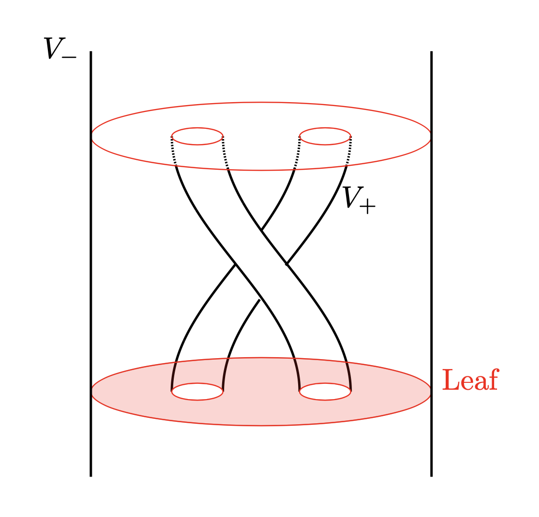
(a) The building block $V$.

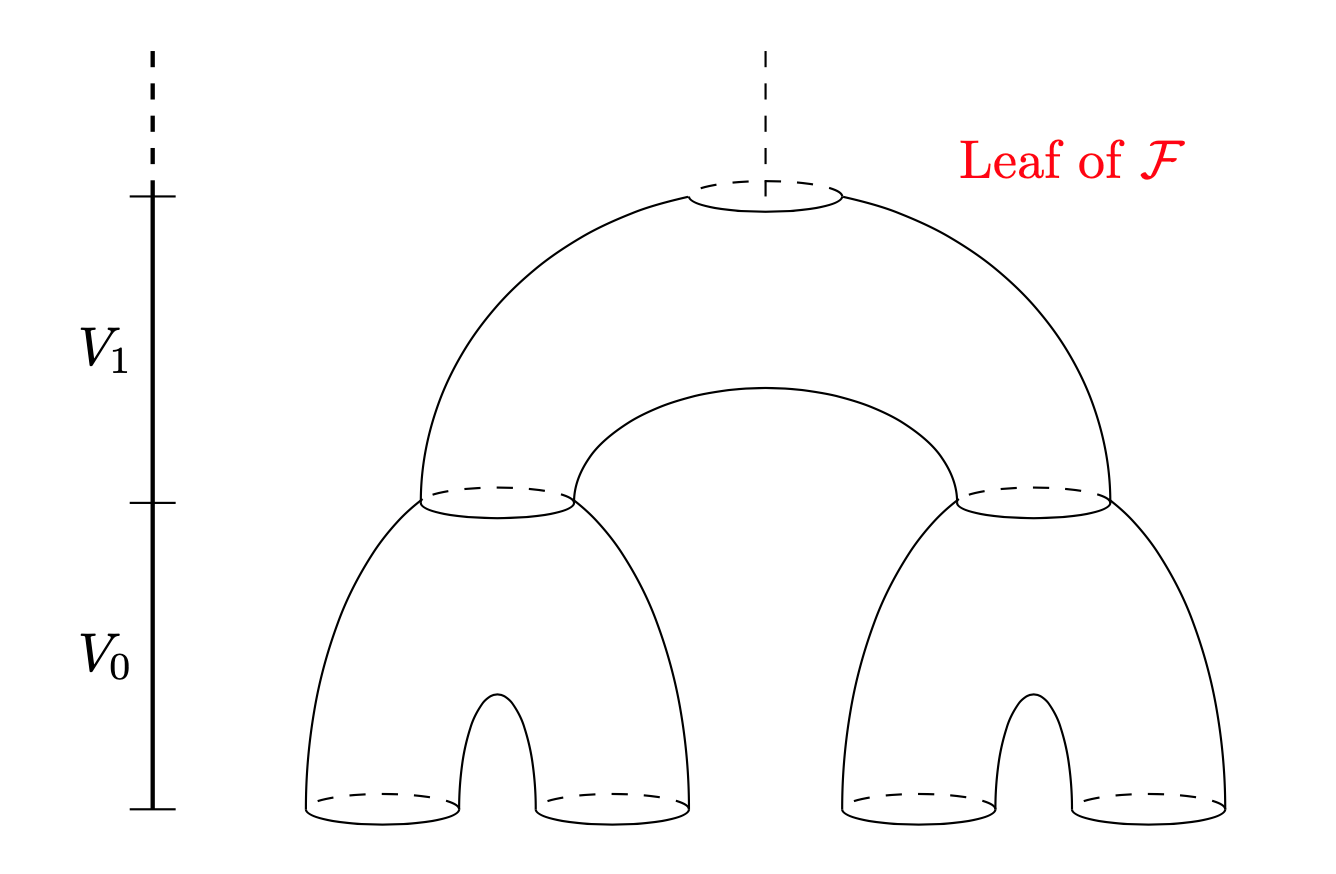
(b) A leaf of $\mathcal{F}$.

Figure 1: Geometrical illustration of $\mathcal{F}$.

Now, we consider a countable family of building-blocks $(V_{n},V_{n}^{-},V_{n}^{+},\iota_{n},\mathcal{G}_{n},g_{n})$, where $g_{n}$ are analytic metrics over $V_{n}$ satisfying the following property: given two points $x$ and $y$ in a leaf $L$ of $\mathcal{G}_{n}$, the distance of $x$ and $y$ in $L$ is bounded by $4^{-n}$. We denote by $M$ the manifold with boundary given by the union of all $V_{n}$, by identifying $V_{n}^{-}$ with $V_{n+1}^{+}$ via $\iota$, that is, we take the identification $x\in V_{n}^{-}$ equivalent to $\iota(x)\in V_{n+1}^{+}$. This yields an analytic manifold with border, where the border is a torus $M_{0}=V_{0}^{+}=S^{1}\times S^{1}$. This construction induces, furthermore, an analytic foliation $\mathcal{F}$ over the manifold with border $M$ which locally agrees with $\mathcal{G}_{n}$ over each $V_{n}$, because $\pi\circ f=\iota\circ\pi$, cf. figure 1(b). Furthermore, we can define a globally defined $C^{\infty}$ metric $g$ over $M$ by patching the metrics $g_{n}$ via partition of the unit. We may chose such a partition so that $g$ satisfies the following property: given two points $x$ and $y$ in a leaf $L$ of $\mathcal{G}_{n}$, the distance of $x$ and $y$ in $L$ is bounded by $2^{-n}$.

We claim that $\mathcal{F}$ is a non-splittable foliation. Indeed, consider a transverse section $\Sigma=S^{1}\subset M_{0}=S^{1}\times S^{1}$ and let us identify $\Sigma$ with the interval $[0,1]$. Given a point $x\in\Sigma$, denote by $L_{x}$ the leaf passing by $x$. First, consider the foliation $\mathcal{G}_{0}$, and note that, since $f(x)=f(x+1/2)$ and $\mathcal{G}_{0}$ is a foliation by pants, $x+1/2$ also belongs to the leaf $L$, cf. figure 1(b). Since this argument can be iterated over any $\mathcal{G}_{n}$, we get that all points $x+m/2^{n}$ with $m,n\in\mathbb{N}$ belong to $L_{x}$. Moreover, the distance on $L_{x}$ between $x$ and $x+m/2^{n}$ is bounded by:

$$2\cdot\sum_{k=0}^{n}\frac{1}{2^{k}}<4$$

since there exists a path between $x$ and $x+m/2^{n}$, contained in the leaf $L_{x}$, and which is contained in the union of $V_{k}$ with $k<n$, crossing each of these components at most twice. In conclusion, for every $x\in\Sigma$, the intersection of $L_{x}$, the leaf passing through $x$, with $\Sigma$ is a countable and dense set of points invariant by a countable subgroup of rotations, which are pairwise $(\mathcal{F},4)$-related. We infer that $\mathcal{F}$ is a not splittable in $(M,g)$ because there is no measurable set $E\subset\Sigma$ with positive Lebesgue measure whose intersection with each $L_{x}$ (with $x\in\Sigma$) contains only one point.

3 Preliminary results

We gather in this section preliminary results in differential geometry (Section 3.1), geometric control theory (Section 3.2), subanalytic geometry (Section 3.3) and on integrable families of $1$-forms (Section 3.4). All proofs are postponed to Appendix C.

3.1 Reminders of differential geometry

Throughout this section, $M$ is a smooth connected manifold of dimension $n\geq 1$. We refer the reader to [15, 34, 40] for further details on the notions and results presented below and we point out that we follow the sign conventions used in [40].

Lie brackets.

Given a smooth vector field $X$ on $M$ we write $X\cdot f$ or $X(f)$ for the Lie derivative of a smooth function $f:M\rightarrow\mathbb{R}$ with respect to $X$. Then, given two smooth vector fields $X,Y$ on $M$ we define their Lie bracket as the vector field uniquely associated with the derivation $Y\circ X-X\circ Y$, which means that, if in a local set of coordinates $(x_{1},\ldots,x_{n})$ in $M$, the vectors fields $X,Y$ are given by

$$X=\sum_{i=1}^{n}a_{i}\,\partial_{x_{i}},\quad Y=\sum_{i=1}^{n}b_{i}\,\partial_{x_{i}},$$

where $a_{1},\ldots,a_{n},b_{1},\ldots b_{n}$ are smooth scalar functions, then the Lie bracket $[X,Y]$ is the smooth vector field defined as

$$[X,Y]=\sum_{i=1}^{n}c_{i}\,\partial_{x_{i}},$$

where $c_{1},\ldots,c_{n}$ are the smooth scalar functions given by

$$c_{i}=\sum_{j=1}^{n}\left(\partial_{x_{j}}a_{i}\right)b_{j}-\left(\partial_{x_{j}}b_{i}\right)a_{j}\qquad\forall i=1,\ldots,n.$$

Symplectic structure of the cotangent bundle.

We equip the cotangent bundle $T^{*}M$ of $M$ with the canonical symplectic form $\omega$ defined as $\omega=-d\lambda$ where $\lambda$ is the canonical Liouville form. This means that if we have a local chart $(x,p)$ of $T^{*}M$ valued in $\mathbb{R}^{n}\times(\mathbb{R}^{n})^{*}$ with coordinates $(x_{1},\ldots,x_{n},p_{1},\ldots,p_{n})$, then $\lambda,\omega$ read

$$\lambda=\sum_{i=1}^{n}p_{i}\,dx_{i}\quad\mbox{and}\quad\omega=\sum_{i=1}^{n}dx_{i}\wedge dp_{i},$$

where the latter amounts to say that we have in local coordinates at ${\mathfrak{a}}\in T^{*}M$,

$$\omega_{{\mathfrak{a}}}(\zeta,\zeta^{\prime})=\sum_{i=1}^{n}\left(\xi_{j}\eta_{j}^{\prime}-\xi_{j}^{\prime}\eta_{j}\right)\qquad\forall\zeta=(\xi,\eta),\zeta^{\prime}=(\xi^{\prime},\eta^{\prime})\in T_{{\mathfrak{a}}}\left(T^{*}M\right).$$

In the paper, we generally denote by ${\mathfrak{a}}$ an element of $T^{*}M$ and we may write ${\mathfrak{a}}=(x,p)$ and $\zeta=(\xi,\eta)$ any element respectively of $T^{*}M$ and $T_{{\mathfrak{a}}}(T^{*}M)$ in local coordinates.

Hamiltonian vector fields and Poisson brackets.

Given a smooth function, called Hamiltonian, $h:T^{*}M\rightarrow\mathbb{R}$ the Hamiltonian vector field associated with it with respect to $\omega$ is the unique smooth vector field $\vec{h}$ on $T^{*}M$ satisfying

$$\imath_{\vec{h}}\omega=dh,$$

which in a set of local coordinates $(x,p)$ in $T^{*}M$ where $\omega=\sum_{i=1}^{n}dx_{i}\wedge dp_{i}$ reads

$$\vec{h}(x,p)=\left(\frac{\partial h}{\partial p}(x,p),-\frac{\partial h}{\partial x}(x,p)\right).$$

By construction, $\vec{h}\cdot h=dh(\vec{h})=\omega(\vec{h},\vec{h})=0$, so $h$ is a first integral of $\vec{h}$ or in other words $h$ is constant along the orbits of $\vec{h}$. Given two smooth Hamiltonians $h,h^{\prime}:T^{*}M\rightarrow\mathbb{R}$, their Poisson bracket is the smooth Hamiltonian $\{h,h^{\prime}\}$ defined by

$$\left\{h,h^{\prime}\right\}:=\omega\bigl{(}\vec{h},\vec{h}^{\prime}\bigr{)},$$

it satisfies by construction

$$\vec{h}^{\prime}\cdot h=dh\bigl{(}\vec{h}^{\prime}\bigr{)}=\omega\bigl{(}\vec{h},\vec{h}^{\prime}\bigr{)}=\left\{h,h^{\prime}\right\}.$$ (3.1)

If $X$ is a given smooth vector field on $M$, then the smooth Hamiltonian $h^{X}:T^{*}M\rightarrow\mathbb{R}$ associated with $X$ on $T^{*}M$ is defined by

$$h^{X}(x,p):=p\cdot X(x)$$

in a set of local coordinates $(x,p)$ in $T^{*}M$ and the associated Hamiltonian vector field is given by

$$\vec{h}^{X}(x,p)=\left(\frac{\partial h^{X}}{\partial p}(x,p),-\frac{\partial h^{X}}{\partial x}(x,p)\right)=\Bigl{(}X(x),-p\cdot d_{x}X\Bigr{)}.$$

The Poisson and Lie brackets are related by the following formula:

Proposition 3.1.

If $X$ and $Y$ are two smooth vector field on $M$, then we have

$$\left\{h^{X},h^{Y}\right\}=h^{[X,Y]}.$$

The proof of Proposition 3.1 is left to the reader.

Isotropic spaces and submanifolds.

For every ${\mathfrak{a}}\in T^{\ast}M$ and every vector space $W\subset T_{{\mathfrak{a}}}(T^{\ast}M)$, we denote by $W^{\omega}$ the symplectic complement of $W$,

$$W^{\omega}:=\Bigl{\{}\zeta\in T_{{\mathfrak{a}}}(T^{*}M)\,|\,\omega_{{\mathfrak{a}}}(\zeta,\zeta^{\prime})=0,\,\forall\zeta^{\prime}\in W\Bigr{\}},$$

and we call $W$ isotropic if $W\subset W^{\omega}$. If $\mathcal{S}$ is a smooth submanifold of $T^{*}M$, we denote by $\omega_{|\mathcal{S}}$ the $2$-form given by the restriction of $\omega$ to $\mathcal{S}$, its kernel at ${\mathfrak{a}}\in\mathcal{S}$ given by

$$\mbox{ker}\left(\omega_{|\mathcal{S}}\right)_{{\mathfrak{a}}}=\Bigl{\{}\zeta\in T_{{\mathfrak{a}}}\mathcal{S}\,|\,\omega_{{\mathfrak{a}}}(\zeta,\zeta^{\prime})=0,\,\forall\zeta^{\prime}\in T_{{\mathfrak{a}}}\mathcal{S}\Bigr{\}}=\left(T_{{\mathfrak{a}}}\mathcal{S}\right)^{\omega}\cap T_{{\mathfrak{a}}}\mathcal{S},$$

is an isotropic space. The following result will be one of the key results in the proof of Theorem 1.5, its proof is given in Appendix C.1:

Proposition 3.2.

Let $\mathcal{S}$ be a smooth submanifold of $T^{*}M$ of dimension $s$, ${\mathfrak{a}}\in\mathcal{S}$, $E\subset T_{{\mathfrak{a}}}\mathcal{S}$ a vector space such that

$$T_{{\mathfrak{a}}}\mathcal{S}=E\oplus\mbox{\em ker}\left(\omega_{|\mathcal{S}}\right)_{{\mathfrak{a}}},$$ (3.2)

and let $r:=\dim\mbox{\em ker}(\omega_{|\mathcal{S}})_{{\mathfrak{a}}}$, then the following properties hold:

• $r\leq\min\{2n-s,s\}$ and $s-r=2l$ for some integer $l$.

• The form $(\omega_{|\mathcal{S}}^{l})_{{\mathfrak{a}}}$ is a volume form over $E$, which means that there is a basis $\{\zeta_{1},\zeta_{1}^{\prime},\ldots,\zeta_{l},\zeta_{l}^{\prime}\}$ of $E$ such that $\omega^{l}_{{\mathfrak{a}}}(\zeta_{1},\zeta_{1}^{\prime},\ldots,\zeta_{l},\zeta_{l}^{\prime})\neq 0$.

• $(\omega_{|\mathcal{S}}^{l+1})_{{\mathfrak{a}}}=0$.

Finally, we say that a smooth submanifold $\mathcal{S}$ of $T^{*}M$ is isotropic if all its tangent spaces are isotropic.

Foliations.

Let $N$ be a smooth manifold of dimension $n\geq 1$, a smooth foliation $\mathcal{F}$ on $N$ of dimension $d\geq 1$ is a smooth atlas $\{(U_{\beta},\varphi_{\beta})\}_{\beta}$ satisfying the following properties:

• For every $\beta$, there are open disks $V^{d}_{\beta}\subset\mathbb{R}^{d}$ and $V^{n-d}_{\beta}\subset\mathbb{R}^{n-d}$ such that the map $\varphi_{\beta}:U_{\beta}\rightarrow V^{d}_{\beta}\times V^{n-d}_{\beta}$ is a smooth diffeomorphism.

• For every $\beta,\beta^{\prime}$ with $U_{\beta}\cap U_{\beta^{\prime}}\neq\emptyset$, the change of coordinates

  $$\varphi_{\beta^{\prime}}\circ\varphi_{\beta}^{-1}\,:\,\varphi_{\beta}(U_{\beta}\cap U_{\beta^{\prime}})\,\longrightarrow\,\varphi_{\beta^{\prime}}(U_{\beta}\cap U_{\beta^{\prime}})$$

  preserves the leaves, which means that it has the form

  $$\bigl{(}\varphi_{\beta^{\prime}}\circ\varphi_{\beta}^{-1}\bigr{)}(x,y)=\bigl{(}h_{1}(x,y),h_{2}(y)\bigr{)}\qquad\forall(x,y)\in\varphi_{\beta}(U_{\beta}\cap U_{\beta^{\prime}}),$$

  for some smooth functions $h_{1},h_{2}$.

A chart $(U_{\beta},\varphi_{\beta})$ is called a foliation chart and any set of the form $\varphi_{\beta}^{-1}(V_{\beta}^{d}\times\{y\})$ with $y\in V^{n-d}_{\beta}$ is called a plaque of the foliation. Then, we can define an equivalence relation on $N$ by saying that two points $z,z^{\prime}$ are equivalent if they can be connected by a path of plaques $P_{1},\ldots,P_{k}$ such that $P_{j}\cap P_{j+1}\neq\emptyset$ for all $j\in\{1,\ldots,k-1\}$. Therefore, $N$ can be partitioned into equivalent classes, called leaves, each of which having the structure of an injectively immersed smooth submanifold of $N$ of dimension $d$. Smooth foliations are indeed in one-to-one correspondence with involutive smooth distributions. Recall that a smooth regular distribution $D$ on $N$, that is, a distribution of constant rank parametrized locally by smooth vector fields, is called involutive if given two smooth vector fields $X,Y$ such that $X(z),Y(z)\in D(z)$ for all $z\in N$, then $[X,Y](z)\in D(z)$ for all $z\in N$. On the one hand, the field of vector spaces corresponding to the tangent spaces to the leaves of a smooth foliation $\mathcal{F}$ forms an involutive distribution, and on the other hand, the Frobenius Theorem asserts that any involutive smooth distribution is integrable, which means that it can be viewed as the tangent plane field of a smooth foliation. If a foliation chart $(U_{\beta},\varphi_{\beta})$ as above is given then the local distribution associated with the foliation is given by the pull-back of the horizontal constant distribution $\mathbb{R}^{k}\times\{0\}$ in $V^{d}_{\beta}\times V^{n-d}_{\beta}$.

As the next result shows, the kernel of the restriction of a symplectic form to a submanifold gives rise to isotropic foliations.

Proposition 3.3.

Let $\mathcal{S}$ be a smooth submanifold of $T^{*}M$ such that the dimension of $\mbox{ker}(\omega_{|\mathcal{S}})\subset T\mathcal{S}$ is constant. Then the smooth distribution

$$\vec{\mathcal{I}}({\mathfrak{a}}):=\mbox{\em ker}\left(\omega_{|\mathcal{S}}\right)_{{\mathfrak{a}}}\qquad\forall{\mathfrak{a}}\in\mathcal{S},$$

is integrable with isotropic leaves.

The proof of Proposition 3.3 is postponed to Appendix C.2.

3.2 Singular horizontal paths and abnormal lifts

Throughout this section, $M$ is a smooth connected manifold of dimension $n\geq 3$ equipped with a totally nonholonomic distribution $\Delta$ of constant rank $m\leq n$. Let us consider a family of smooth vector fields $X^{1},\ldots,X^{k}$ with $m\leq k\leq m(m+1)$ (see [53, 58]) providing a global parametrization of $\Delta$ over $M$, that is, satisfying

$$\Delta(x)=\mbox{Span}\Bigl{\{}X^{1}(x),\ldots,X^{k}(x)\Bigr{\}}\qquad\forall x\in M.$$

Then, define the distribution $\vec{\Delta}$ on $T^{*}M$ by

$$\vec{\Delta}({\mathfrak{a}}):=\Bigl{\{}\vec{h}^{1}({\mathfrak{a}}),\ldots,\vec{h}^{k}({\mathfrak{a}})\Bigr{\}}\qquad\forall\,{\mathfrak{a}}\in T^{*}M,$$

where for every $i=1,\ldots,k$, $h^{i}$ stands for the Hamiltonian $h^{X^{i}}:T^{*}M\rightarrow\mathbb{R}$ associated with $X^{i}$. By construction, $\vec{\Delta}$ is a smooth distribution of rank $m$ which projects onto $\Delta$, that is, such that $\pi_{*}(\vec{\Delta})=\Delta$ where $\pi:T^{*}M\to M$ is the canonical projection. In order to give several characterizations of the notion of singular horizontal path, it is useful to identify the horizontal paths with the trajectories of a control system and to define the so-called end-point mapping. It is important to note that all results presented below are classical, we refer the reader to [2, 45, 53] for further details.

The End-Point mapping.

For every $x\in M$, there is a non-empty maximal open set $\mathcal{U}^{x}\subset L^{2}([0,1],\mathbb{R}^{k})$ such that for every control $u=(u_{1},\cdots,u_{k})\in\mathcal{U}^{x}$, the solution $x(\cdot;x,u):[0,1]\rightarrow M$ to the Cauchy problem

$$\dot{x}(t)=\sum_{i=1}^{k}u_{i}(t)X^{i}(x(t))\quad\mbox{for a.e. }t\in[0,1]\quad\mbox{and}\quad x(0)=x$$ (3.3)

is well-defined. By construction, for every $x\in M$ and every control $u\in\mathcal{U}^{x}$ the trajectory $x(\cdot;x,u)$ is an horizontal path in $\Omega_{\Delta}^{x}$, the set of horizontal paths $\gamma:[0,1]\rightarrow M$ in $W^{1,2}([0,1],M)$ with $\gamma(0)=x$. Moreover, the converse is true, any $\gamma\in\Omega_{\Delta}^{x}$ can be written as the solution of (3.3) for some $u\in\mathcal{U}^{x}$. Of course, since in general the vector fields $X^{1},\ldots,X^{k}$ are not linearly independent globally on $M$, the control $u$ such that $\gamma=x(\cdot;x,u)$ is not necessarily unique. For every point $x\in M$, the End-Point Mapping from $x$ (associated with $X^{1},\ldots,X^{k}$ in time $1$) is defined as

$$\begin{array}[]{rcl}\mbox{E}^{x}:\mathcal{U}^{x}&\longrightarrow&M\\ u&\longmapsto&x(1;x,u).\end{array}$$

It shares the same regularity as the vector fields $X^{1},\ldots,X^{k}$, it is of class $C^{\infty}$. Given $x\in M$ and $u\in\mathcal{U}^{x}\subset L^{2}([0,1],\mathbb{R}^{k})$, we define the rank of $u$ with respect to $E^{x}$ by

$$\mbox{rank}(u):=\dim\left(\mbox{Im}\left(d_{u}E^{x}\right)\right),$$

where $\mbox{Im}\left(d_{u}E^{x}\right)$ denotes the image of the differential of $E^{x}$ at $u$

$$d_{u}E^{x}\,:\,L^{2}\left([0,1],\mathbb{R}^{k}\right)\longrightarrow T_{E^{x}(u)}M.$$

It can be shown that for every $u\in\mathcal{U}^{x}$, one has (see [53, Proposition 1.10 p. 19])

$$\Delta\left(E^{x}(u)\right)\subset\mbox{Im}\left(d_{u}E^{x}\right),$$ (3.4)

in such a way that $\mbox{rank}(u)\geq m$ for all $u\in\mathcal{U}^{x}$. Then, we define the rank of a horizontal path $\gamma\in\Omega_{\Delta}^{x}$, denoted by $\mbox{rank}^{\Delta}(\gamma)$, as the rank of any control $u\in\mathcal{U}^{x}$ such that $\gamma=x(\cdot;x,u)$, and the corank of $\gamma$ (with respect to $\Delta$) by $\mbox{corank}^{\Delta}(\gamma):=n-\mbox{rank}^{\Delta}(\gamma)$. It can be shown that the rank defined in this way does not depend neither on the control $u$ satisfying $\gamma=x(\cdot;x,u)$ nor on the family $X^{1},\ldots,X^{k}$ used to parametrize $\Delta$. A horizontal path $\gamma:[0,1]\rightarrow M$ is said to be singular if its rank is strictly less than $n$ and it is said to be of minimal rank if $\mbox{rank}^{\Delta}(\gamma)=m$.

Characterizations of singular horizontal paths.

Recall that $\Delta^{\perp}$ denotes the smooth submanifold of $T^{*}M$ of codimension $m$ given by the set of non-zero annihilators of $\Delta$ in $T^{*}M$. The following result provides several characterizations of singular curves such as Hsu’s characterization used in the introduction of the paper, its proof is recalled in Appendix C.3:

Proposition 3.4.

Let $\gamma:[0,1]\rightarrow M$ be an absolutely continuous curve which is horizontal with respect to $\Delta$, let $u\in\mathcal{U}^{x}$, with $x:=\gamma(0)$, be such that $\gamma=x(\cdot;x,u)$, and let $p\in T_{y}^{*}M\setminus\{0\}$, with $y:=\gamma(1)$, be fixed. Then the following properties are equivalent:

• $p\in\left(\mbox{\em Im}\left(d_{u}E^{x}\right)\right)^{\perp}$.

• There is an absolutely continuous curve $\psi:[0,1]\rightarrow\Delta^{\perp}$ which is horizontal with respect to $\vec{\Delta}$ such that $\pi(\psi)=\gamma$ and $\psi(1)=(y,p)$.

• There is an abnormal lift $\psi:[0,1]\rightarrow\Delta^{\perp}$ of $\gamma$ with $\psi(1)=(y,p)$, that is, an absolutely continuous curve $\psi:[0,1]\rightarrow\Delta^{\perp}$ with $\psi(1)=(y,p)$ such that $\pi(\psi)=\gamma$ and $\dot{\psi}(t)\in\mbox{\em ker}(\omega^{\perp}_{\psi(t)})$ for almost every $t\in[0,1]$.

In particular, $\mbox{rank}^{\Delta}(\gamma)\in[m,n]$ and $\gamma$ is singular ($\mbox{rank}^{\Delta}(\gamma)<n$) if and only if it admits an abnormal lift. Moreover, any absolutely continuous curve $\psi:[0,1]\rightarrow\Delta^{\perp}$ satisfying the property of (iii) is an abnormal lift and if $\gamma$ has minimal rank ($\mbox{rank}^{\Delta}(\gamma)=m$) then for each $p\in(\Delta^{\perp})_{x}$ there is an abnormal lift $\psi:[0,1]\rightarrow\Delta^{\perp}$ of $\gamma$ such that $\psi(1)=(y,p)$.

The part of Proposition 3.4 establishing that abnormal lifts of a given horizontal path do coincide with lifts which are tangent to $\vec{\Delta}$ in $\Delta^{\perp}$ is a consequence of the following equality

$$\mbox{ker}\bigl{(}\omega^{\perp}_{{\mathfrak{a}}}\bigr{)}=\bigl{(}T_{{\mathfrak{a}}}\Delta^{\perp}\bigr{)}^{\omega}\cap\,T_{{\mathfrak{a}}}\Delta^{\perp}=\vec{\Delta}({\mathfrak{a}})\cap\,T_{{\mathfrak{a}}}\Delta^{\perp}\qquad\forall{\mathfrak{a}}\in\Delta^{\perp}.$$ (3.5)

This approach allows also to relate the kernel of $\omega^{\perp}$ to the kernel of some linear operator defined from Poisson brackets of length two. Assume now that, in an open neighborhood $\mathcal{V}$ of some $x\in M$, $\Delta$ is generated by $m$ smooth vector fields $X^{1},\ldots,X^{m}$. Then, set $h^{i}:=h^{X^{i}}$ for all $i=1,\ldots,m$ and define the Hamiltonians $h^{ij}$ with $i,j\in\{1,\ldots,m\}$ by

$$h^{ij}:=\left\{h^{i},h^{j}\right\},$$

which by (3.1) and Proposition 3.1 satisfy

$$h^{ij}=\vec{h^{j}}\cdot h^{i}=h^{[X^{i},X^{j}]}.$$ (3.6)

We have the following result whose proof is given in Appendix C.4:

Proposition 3.5.

For every ${\mathfrak{a}}\in T^{*}\mathcal{V}\cap\Delta^{\perp}$, define $\mathcal{L}^{2}_{{\mathfrak{a}}}:\vec{\Delta}({\mathfrak{a}})\rightarrow\mathbb{R}^{m}$ by

$$\left(\mathcal{L}^{2}_{{\mathfrak{a}}}(\zeta)\right)_{i}:=\sum_{j=1}^{m}u_{j}\,h^{ij}({\mathfrak{a}})\qquad\forall\zeta=\sum_{i=1}^{m}u_{i}\vec{h}^{i}({\mathfrak{a}})\in\vec{\Delta}({\mathfrak{a}}),\,\forall i=1,\ldots,m.$$

Then, for every ${\mathfrak{a}}\in T^{*}\mathcal{V}\cap\Delta^{\perp}$, we have $\mbox{\em ker}(\mathcal{L}^{2}_{{\mathfrak{a}}})=\mbox{\em ker}(\omega^{\perp}_{{\mathfrak{a}}})$.

Finally, Propositions 3.4 and 3.5 allow us to show that singular horizontal paths with minimal rank are constrained to be tangent to a (singular) distribution on $M$. Recalling that $\pi:T^{*}M\rightarrow M$ stands for the canonical projection and that $\Delta^{\perp}_{x}:=T_{x}^{*}M\cap\Delta^{\perp}$ denotes the fiber in $\Delta^{\perp}$ over some $x\in M$, we have:

Proposition 3.6.

Let $\gamma:[0,1]\rightarrow M$ be a singular horizontal path with respect to $\Delta$. Then $\gamma$ has minimal rank if and only if

$$\dot{\gamma}(t)\in\bigcap_{{\mathfrak{a}}\in\Delta^{\perp}_{\gamma(t)}}\pi_{*}\left(\mbox{\em ker}\bigl{(}\omega^{\perp}_{{\mathfrak{a}}}\bigr{)}\right)\qquad\mbox{for a.e. }t\in[0,1].$$ (3.7)

The proof of the above result is given in Appendix C.5.

3.3 Reminders of subanalytic geometry

We recall here the main notions of subanalytic geometry used in this paper. We refer the reader to [11, 26, 38] for further details. Throughout this section, $N$ stands for a real-analytic connected manifold of dimension $n$. Later on, $N$ will stand for one of the following three manifolds: $M$, $T^{\ast}M$ or $\Delta^{\perp}$.

Subanalytic sets.

Let $d$ be a nonnegative integer. An analytic submanifold $S$ of dimension $d$ of $N$ is an embedded submanifold such that for every point $p\in S$ there are a neighborhood $U\subset N$ and $n-d$ analytic functions $f_{1},\ldots,f_{n-d}:U\rightarrow\mathbb{R}$ with the property that $df_{1},\ldots,df_{n-d}$ are linearly independent over $U$ and $S\cap U$ is the set of points where all the $f_{i}$ vanish. A set $X\subset N$ is said to be analytic if for every $x\in N$ there is an open neighborhood $U$ of $x$ in $N$, and a real-analytic function $f:U\to\mathbb{R}$ such that $X\cap U=\{f=0\}$. Note that every closed analytic submanifold is an analytic set locally given by $\{f_{1}^{2}+\ldots+f_{n-d}^{2}=0\}$. Similarly, a set $X\subset N$ is said to be semianalytic if for every $x\in N$, there is an open neighborhood $U$ of $x$ in $N$ and a finite number of real-analytic functions $f_{i}:U\to\mathbb{R}$ and $g_{ij}:U\to\mathbb{R}$ with $j=1,\ldots,b_{i}$ and $i=1,\ldots,a$ such that

$$X\cap U=\bigcup_{i=1}^{a}\left\{y\in U;\,f_{i}(y)=0;\,g_{i1}(y)>0,\ldots,g_{ib_{i}}(y)>0\right\}.$$

It is worth noting that an analytic submanifold $S$ is not necessarily a semianalytic set, unless $S$ is closed. By definition, the class of semianalytic sets is closed by the operations of locally finite unions, locally finite intersections, and taking the complement. Moreover, it can be shown that it is also stable by closure (the closure of a semianalytic set is semianalytic) and connected component (each connected component of a semianalytic set is semianalytic). However the image of a semianalytic set by an analytic map, even a proper one, is not necessarily semianalytic.

A set $X\subset N$ is called subanalytic if for every $x\in N$, there is an open neighborhood $U$ of $x$ in $N$ and a relatively compact semianalytic set $Y\subset M\times\mathbb{R}^{k}$ (where $k$ may depend on $x$) such that $X\cap U$ is the image of $Y$ by the canonical projection $M\times\mathbb{R}^{k}\rightarrow N$. The class of subanalytic sets is closed by the operations of locally finite unions, locally finite intersections and taking the complement (by a theorem of Gabrielov), and stable by closure and connected component. Moreover, the image of a relatively compact subanalytic set by an analytic map is subanalytic.

Whitney’s stratification and uniformization.

We recall here two important techniques of subanalytic geometry which are used in the paper: Whitney subanalytic stratification and the uniformization Theorem. We refer the reader to [22, 11] for a complete introduction on these two techniques.

Let $N$ be a smooth manifold and $Z$ be a closed subset of $N$. We call Whitney stratification of $Z$ any partition $\mathcal{S}=(\mathcal{S}_{\alpha})$ of $Z$ into locally closed smooth submanifolds $\mathcal{S}_{\alpha}$, called strata of $\mathcal{S}$, that is,

$$Z=\bigsqcup_{\mathcal{S}_{\alpha}\in\mathcal{S}}\mathcal{S}_{\alpha},$$

such that the following properties are satisfied:

• The family $\mathcal{S}$ is locally finite.

• If $S\in\mathcal{S}$ then the closure $\bar{S}$ of $S$ is the union of those strata that intersect $\bar{S}$.

• If $S,T$ are strata with $T\neq S$ and $T\subset\bar{S}$, then $\mbox{dim}(T)<\mbox{dim}(S)$.

• Let $S,T$ be two strata with $T\neq S$ and $T\subset\bar{S}$, let $\{x_{k}\}_{k}\in S$ and $\{y_{k}\}_{k}\in T$ be sequences of points converging to a point $y\in T$:

  • (Whitney condition a) If the tangent spaces $T_{x_{k}}S$ converge to a vector subspace $\tau\subset T_{y}N$, then $T_{y}T\subset\tau$.

  • (Whitney condition b) If the secant lines $\ell_{k}=(x_{k}y_{k})$, with respect to some local coordinate system on $N$, converge to a line $\ell\subset T_{y}N$, then $\ell\subset\tau$.

A stratification $\mathcal{S}$ is said to be compatible with a family $\mathcal{A}$ of subsets of $N$ if every $A\in\mathcal{A}$ is a union of strata of $\mathcal{S}$. A stratification $\mathcal{S}^{\prime}$ is a refinement of $\mathcal{S}$ if it is compatible with all strata of $\mathcal{S}$. A Whitney analytic stratification, or simply analytic stratification, is a stratification whose strata are connected real-analytic submanifolds. A Whitney subanalytic stratification of $N$ is an analytic stratification $\mathcal{S}$ such that all the strata of $\mathcal{S}$ are subanalytic. We start by noting that all subanalytic sets admit a subanalytic Whitney stratification:

Theorem 3.7 (Whitney subanalytic stratification).

Let $N$ be a real-analytic manifold and $\mathcal{A}$ be a locally finite collection of subanalytic sets of $N$. Then there exists a Whitney subanalytic stratification of $N$ compatible with $\mathcal{A}$.

Now, given a subanalytic set $X\subset N$ and a subanalytic stratification $\mathcal{S}=(\mathcal{S}_{\alpha})$ of $X$, the dimension of $X$ is defined as the highest dimension of strata $S\in\mathcal{S}$. Now that we have defined the notion of dimension, we can present the uniformization Theorem:

Theorem 3.8 (Uniformization).

Let $N$ be an analytic manifold and $X$ be a closed subanalytic subset of $N$. Then there exists an analytic manifold $W$ of the same dimension as $X$ and a proper analytic map $\Phi:W\to N$ such that $\Phi(W)=X$.

Subanalytic distributions and foliations.

A distribution $\Delta$ of $N$ is said to be subanalytic if its graph in $TN$ is a subanalytic set. As stated in the introduction, the dimension of the vector space $\Delta(x)=\Delta\cap T_{x}N$ is called the rank of $\Delta$ at $x$.

Given a subanalytic stratification $\mathcal{S}=(\mathcal{S}_{\alpha})_{\alpha}$ of $N$, we say that $\Delta$ is compatible with $\mathcal{S}$, or that $\mathcal{S}$ is compatible with $\Delta$, if for every stratum $\mathcal{S}_{\alpha}$, the rank of $\Delta$ is constant along $\mathcal{S}_{\alpha}$ and $\Delta\cap T\mathcal{S_{\alpha}}$ is an analytic vector-bundle over $\mathcal{S}_{\alpha}$. The following result, whose proof is postponed to Appendix $\S$C.6, shows that for every subanalytic distribution $\Delta$, there exists a subanalytic stratification $\mathcal{S}$ which is compatible with $\Delta$.

Proposition 3.9.

Let $\Delta\subset TN$ be a closed subanalytic distribution. There exists a subanalytic Whitney stratification $\mathcal{S}=(\mathcal{S}_{\alpha})$ of $N$ such that:

1. the rank of $\Delta$ is constant along $\mathcal{S}_{\alpha}$;

2. $\Delta\cap T\mathcal{S}_{\alpha}$ is an analytic vector-bundle over $\mathcal{S}_{\alpha}$ for each $\alpha$.

Furthermore, if $\mathcal{S}^{\prime}$ is a subanalytic stratification of $N$, then $\mathcal{S}$ can be chosen as a refinement of $\mathcal{S}^{\prime}$.

Suppose that $\Delta$ is compatible with a Whitney stratification $\mathcal{S}$. We say that $\Delta$ is integrable at $x\in N$ if the Lie-bracket closure of $\Delta\cap T\mathcal{S}_{\alpha}$ at $x$, where $x\in S_{\alpha}$, is equal to $\Delta\cap T\mathcal{S}_{\alpha}$. Then, we say that $\Delta$ is integrable if it is integrable at every point. Now, recall that a smooth integrable distribution $\Delta$ of constant rank generates a smooth foliation $\mathcal{F}$, see $\S\S$3.1. If $\Delta$ is integrable and subanalytic, then we say that the induced foliation $\mathcal{F}=(\mathcal{F}_{\alpha})$ is a subanalytic foliation.

3.4 Integrable families of 1-forms

We recall here the main notions of analytic geometry, in particular of Pfaffian systems, used in this work. We start with the case of families of $1$-forms on an open and connected set $U\subset\mathbb{R}^{n}$. Let $\Omega=\{\omega_{1},\ldots,\omega_{t}\}$ be a family of analytic $1$-forms on $U$, that is, such that each $\omega_{k}$ ($k=1,\ldots,t$) has the form

$$\omega_{k}=a_{k,1}(x)dx_{1}+\cdots+a_{k,n}(x)dx_{n}\qquad\forall k=1,\ldots,t,$$

for some analytic functions $a_{k,1},\ldots,a_{k,n}$ on $U$. Consider the analytic distribution $\mathcal{K}_{\Omega}$ given by

$$\mathcal{K}_{\Omega}(x):=\bigcap_{k=1}^{t}\mbox{ker}\left((\omega_{k})_{x}\right)\qquad\forall x\in U$$

and denote by $r$ its generic corank and by $\Sigma\subset U$ the analytic set, called singular set of $\Omega$, of points where the corank of $\mathcal{K}_{\Omega}$ is strictly smaller than $r$. Then, we say that $\Omega$ is integrable if there holds

$$d\omega_{k}\in\Omega\wedge\Omega_{U}^{1}\qquad k=1,\ldots,t,$$

where $\Omega_{U}^{1}$ stands for the module of analytic $1$-forms defined on $U$. It follows from Frobenius Theorem, see e.g. [50, Th.2.9.11], that if $\Omega$ is integrable, then $\mathcal{K}_{\Omega}$ is integrable distribution over $U\setminus\Sigma$ and generates an analytic foliation $\mathcal{F}_{|U\setminus\Sigma}$ (as we will see in Remark 3.10 below, $\Omega$ actually generates a subanalytic foliation). Then, we consider the dual of $\Omega$, that is, the set of analytic vector fields $X$ on $U$ satisfying

$$\imath_{X}\omega_{k}\equiv 0\qquad\forall k=1,\ldots,t.$$

By construction, this collection of vector fields $\Omega^{\ast}$ generates a module of analytic vector fields and moreover, outside of $\Sigma$, the analytic distribution generated by $\Omega^{\ast}$ is equal to $\mathcal{K}_{\Omega}$ (although this might not be true over $\Sigma$).

The above definitions can be made global over an analytic manifold $N$ via sheaves. Denoting by $\mathcal{O}_{N}$ the sheaf of analytic functions over $N$ and by $\Omega_{N}^{1}$ the sheaf of analytic $1$-forms over $N$, we can consider sub-sheaves $\Omega\subset\Omega_{N}^{1}$ of finite type, that is, locally generated by a finite family of analytic $1$-forms as above, and extend all above notions to this setting.

Given an analytic map $f:Z\to N$, where $Z$ is an analytic manifold, the differential of $f$ induces a natural map between forms

$$\begin{matrix}f^{\ast}\,:\,&\Omega_{N}^{1}&\longrightarrow&\Omega_{Z}^{1}\\ &\alpha&\longmapsto&f^{\ast}\alpha,\end{matrix}$$

where $f^{\ast}\alpha_{x}(X)=\alpha_{f(x)}(df\cdot X)$ for all point $x\in Z$ and all vector field germ $X\in\mbox{Der}_{Z,x}$. The pull-back $f^{\ast}\Omega$ of $\Omega$ is the sub-sheaf of $\Omega^{1}_{Z}$ generated by the image of $f^{\ast}(\Omega)$.

Remark 3.10.

Of particular importance is the case that $Z$ is a submanifold of $N$ and $f$ is the embedding. If $\Omega$ is integrable, then so is $f^{\ast}(\Omega)$ since

$$df^{\ast}(\omega)=f^{\ast}(d\omega)\in f^{\ast}\left(\Omega\wedge\Omega^{1}_{N}\right)\subset f^{\ast}(\Omega)\wedge\Omega^{1}_{Z}.$$

Note that the generic corank of $f^{\ast}(\Omega)$ is always smaller than or equal to the generic corank of $\Omega$. Therefore, given an integrable sheaf of $1$-forms $\Omega$ and a Whitney stratification $\mathcal{S}$ compatible with the distribution $\mathcal{K}_{|\Omega}$, then $\mathcal{K}_{|\Omega}$ yields a subanalytic foliation $(\mathcal{F}_{\alpha})$.

Example 3.11.

Let $M=U\subset\mathbb{R}^{n}$ be an open ball and $\Delta$ be an analytic nonholonomic distribution of constant rank $m$. Apart from shirinking $U$, we may suppose that $\vec{\Delta}\subset T(T^{\ast}M)$ is locally generated by analytic Hamiltonian vector fields $\{\vec{h}^{1},\ldots,\vec{h}^{m}\}$, cf. $\S\S$3.2. We may assume that there exists coordinate system $({\mathfrak{a}}_{1},\ldots,{\mathfrak{a}}_{2n})$ of $T^{\ast}M$ such that $\vec{h}^{k}({\mathfrak{a}}_{k})=1$ and $\vec{h}^{k}({\mathfrak{a}}_{j})=0$, for all $j,k=1,\ldots,m$. Let

$$\omega_{l}=\sum_{k=1}^{m}\vec{h}^{k}({\mathfrak{a}}_{l})d{\mathfrak{a}}_{k}-d{\mathfrak{a}}_{l},\quad l=m+1,\ldots,n,$$

and consider the sheaf of $1$-forms $\Omega_{\vec{\Delta}}$ generated by these forms. It follows from a direct computation that $\mathcal{K}_{\Omega_{\vec{\Delta}}}=\vec{\Delta}$. Moreover, if we denote by $i:\Delta^{\perp}\to T^{\ast}M$ the inclusion, then $i^{\ast}\Omega_{\vec{\Delta}}$ gives rise to a family of Pfaffian equations over $\Delta^{\perp}$, whose associated distribution is equal to $\mbox{ker}(\omega^{\perp})$ by equation (3.5).

4 Proof of Theorem 1.1

Proof of (i).

Since $M$ and $\Delta$ are real-analytic, $\Delta^{\perp}$ (given by (1.1)) is an analytic submanifold of $T^{*}M$ of dimension $2n-m$. As in the introduction, we denote by $\omega$ the canonical symplectic form over $T^{\ast}M$ and by $\omega^{\perp}$ its restriction to $\Delta^{\perp}$. We recall that, since $T^{\ast}M$ is a vector bundle, the dilation in the fibers $\sigma_{\lambda}:T^{\ast}M\to T^{\ast}M$ given by $\sigma_{\lambda}(x,p)=(x,\lambda p)$ for $\lambda\in\mathbb{R}^{\ast}$ are well-defined everywhere in $T^{\ast}M$, which gives rise to a natural structure of projective bundle. More generally, let $G$ denote a group of analytic automorphisms of $\Delta^{\perp}$ such that:

• $G$ contains the dilations $\sigma_{\lambda}$ for $\lambda\in\mathbb{R}^{\ast}$.

• $G$ fixes $\mbox{ker}(\omega^{\perp})$, that is, $d_{{\mathfrak{a}}}\sigma\,(\mbox{ker}(\omega^{\perp}_{{\mathfrak{a}}}))=\mbox{ker}(\omega^{\perp}_{\sigma({\mathfrak{a}})}),$ $\forall\sigma\in G,\,\forall{\mathfrak{a}}\in\Delta^{\perp}$.

• The quotient space $\Delta^{\perp}_{G}$ is an analytic manifold and the geometrical quotient map $\Pi:\Delta^{\perp}\to\Delta^{\perp}_{G}$ is an analytic (and, therefore, subanalytic) submersion.

In general, $G$ stands for the group of dilations (in this case, the above conditions are immediate), but it might stand for a more general group, such as in the case of Carnot groups, cf. $\S\S$2.4. We will say that a set $X\subset\Delta^{\perp}$ is $G$-invariant if $\sigma(X)=X$ for every $\sigma\in G$. In this case, we denote by $X_{G}$ its image by the quotient map, that is $X_{G}=\Pi(X)\subset\Delta^{\perp}_{G}$. Note that if $X$ is a subanalytic $G$-invariant set, then $X_{G}$ is a subanalytic set (since $\Pi$ is an analytic submersion). Reciprocally, if $Y\subset\Delta^{\perp}_{G}$ is subanalytic, then $\Pi^{-1}(Y)\subset\Delta^{\perp}$ is a subanalytic $G$-invariant set (since $\Pi$ is subanalytic and the restriction of the projection $\pi_{1}:\Delta^{\perp}\times\Delta^{\perp}_{G}\to\Delta^{\perp}$ to the graph $\Gamma(\Pi)$ of $\Pi$ is a proper mapping so that $\Pi^{-1}(Y)=\pi_{1}(\Gamma(\Pi)\cap\Delta^{\perp}\times Y)$ is subanalytic). A stratification $\mathcal{S}$ is $G$-invariant if all of its strata are $G$-invariant. We say that a distribution $\vec{\mathcal{K}}$ of $\Delta^{\perp}$ is $G$-invariant if $d\sigma_{{\mathfrak{a}}}\,(\vec{\mathcal{K}}({\mathfrak{a}}))=\vec{\mathcal{K}}(\sigma({\mathfrak{a}}))$ for every ${\mathfrak{a}}\in\Delta^{\perp}$ and $\sigma\in G$; in this case we denote by $\vec{\mathcal{K}}_{G}$ the associated distribution in $\Delta^{\perp}_{G}$, that is, $\vec{\mathcal{K}}_{G}(\Pi({\mathfrak{a}}))=d\Pi_{{\mathfrak{a}}}(\vec{\mathcal{K}}({\mathfrak{a}}))$ which is well-defined since $\Pi\circ\sigma({\mathfrak{a}})=\Pi({\mathfrak{a}})$, so that $d\Pi_{\sigma({\mathfrak{a}})}d\sigma_{{\mathfrak{a}}}=d\Pi_{{\mathfrak{a}}}$. Moreover, if $\vec{\mathcal{K}}$ is subanalytic, then so it $\vec{\mathcal{K}}_{G}$ (because the group $G^{\prime}$ of automorphisms from $T\Delta^{\perp}$ generated by $d\sigma$ for all $\sigma\in G$, is such that $\vec{\mathcal{K}}$ is $G^{\prime}$-invariant and $G^{\prime}$ satisfies property $(G3)$ since $d\Pi:T\Delta^{\perp}\to T\Delta^{\perp}_{G}$ is an analytic submersion). Both $\Delta^{\perp}$ and $\mbox{ker}(\omega^{\perp})$ are $G$-invariant.

Now, we claim that the graph of $\mbox{ker}(\omega^{\perp})$ is a closed subanalytic subset of $T\Delta^{\perp}$. Indeed, this property is local, so we may suppose that $\Delta$ is generated by analytic vector fields $X^{1},\ldots,X^{m}$. This implies that $\vec{\Delta}$ is an analytic distribution, so its intersection with $T\Delta^{\perp}$ is an analytic subset $T\Delta^{\perp}$, and we conclude by equation (3.5). Next, since $\Delta^{\perp}$ is connected and $\omega$ is analytic, there exists $l\in\mathbb{N}$ such that $(\omega^{\perp})^{l+1}\equiv 0$ over $\Delta^{\perp}$ and $(\omega^{\perp})^{l}$ is non-zero over an open dense set $\mathcal{S}_{0}$ of $\Delta^{\perp}$ whose complement is an analytic set; in particular, the rank of $\mbox{ker}(\omega^{\perp})$ is constant along $\mathcal{S}_{0}$. Note that $\mathcal{S}_{0}$ is $G$-invariant. Finally, the existence of the stratification $\mathcal{S}$ and the distributions $\vec{\mathcal{K}}$, $\vec{\mathcal{J}}$ and $\vec{\mathcal{I}}$ follows from the Lemma below applied to $X=\Delta^{\perp}\setminus\mathcal{S}_{0}$:

Lemma 4.1.

Let $M$ and $\Delta$ be real-analytic, and let $X\subset\Delta^{\perp}$ be a $G$-invariant subanalytic set. There exists a $G$-invariant subanalytic Whitney stratification $\mathcal{S}=(\mathcal{S}_{\alpha})$ of $X$ which satisfies the following property: fix a stratum $\mathcal{S}_{\alpha}\subset X$ and consider the distributions $\vec{\mathcal{K}}\subset\vec{\mathcal{J}}\subset\vec{\mathcal{I}}\subset TX$ at a point ${\mathfrak{a}}\in\mathcal{S}_{\alpha}$ given by:

$$\vec{\mathcal{K}}({\mathfrak{a}}):=\ker(\omega^{\perp})({\mathfrak{a}})\cap T_{{\mathfrak{a}}}\mathcal{S}_{\alpha},\quad\vec{\mathcal{J}}({\mathfrak{a}}):=\mbox{\em Lie}(\vec{\mathcal{K}}|_{\mathcal{S}_{\alpha}}({\mathfrak{a}})),\quad\vec{\mathcal{I}}({\mathfrak{a}}):=\mbox{\em Ker}(\omega_{{\mathfrak{a}}}|_{\mathcal{S}_{\alpha}})$$

(in particular, $\vec{\mathcal{K}}$ is an isotropic distribution; $\vec{\mathcal{J}}$ is an integrable distribution and $\vec{\mathcal{I}}$ is an isotropic integrable distribution), then the distributions $\mbox{ker}(\omega^{\perp}),\vec{\mathcal{K}},\vec{\mathcal{J}},\vec{\mathcal{I}}\subset T\Delta^{\perp}$ are subanalytic, $G$-invariant and of constant rank along $\mathcal{S}_{\alpha}$.

Proof of Lemma 4.1.

We prove the result by induction on the dimension of the set $X$, we note that the $0$-dimensional case is obvious. Fix a $G$-invariant subanalytic set $X$ of dimensions $d$. Recall that the projection $\Pi(X)=X_{G}$ is a subanalytic subset of $\Delta^{\perp}_{G}$, and consider a subanalytic Whitney stratification $\mathcal{R}$ of $X_{G}$, see Theorem 3.7. We denote by $\mathcal{S}$ the pre-image of $\mathcal{R}$ by $\Pi$, which is a $G$-invariant subanalytic Whitney stratification of $X$. Denote by $X^{\prime}$ the union of strata of dimension at most $d-1$ and note that it is $G$-invariant. In what follows we show that the Lemma holds over the strata of pure dimension $d$, apart from refining the stratification three times, each time increasing the size, but not the dimension, of $X^{\prime}$. The result will then follow by induction applied to $X^{\prime}$.

Let $r$ denote the rank of $d\Pi$, which is constant since $\Pi$ is a submersion and $\Delta^{\perp}$ is connected. Note that the dimension of $X_{G}$ is equal to $e=d-n+r$. By the uniformization Theorem 3.8, there exists a proper real-analytic mapping $\psi:Z\to X_{G}$, where $Z$ is a smooth manifold of dimension $e$ such that $\psi(Z)=X_{G}$. Denote by $W$ the fiber product

$$W=\Delta^{\perp}\times_{\Delta^{\perp}_{G}}Z,$$

by $\varphi:W\to\Delta^{\perp}$ the projection onto $\Delta^{\perp}$ and by $\Pi^{\prime}:W\to Z$ the projection onto $Z$. We claim that $W$ is a smooth manifold of dimension $d$, and that $\varphi$ is a proper analytic map such that $\varphi(W)=X$. Indeed, since $\Delta^{\perp}$, $\Delta^{\perp}_{G}$ and $Z$ are smooth and $\Pi$ is a submersion, we conclude that $W$ is locally a submanifold of $\Delta^{\perp}\times Z$ of dimension $e+n-r=d$. In particular, we conclude that $W$ is a smooth manifold of dimension $d$, and that $\varphi$ and $\Pi^{\prime}$ are analytic morphisms. Next, the restriction of the projection $\pi_{1}:\Delta^{\perp}\times X_{G}\to\Delta^{\perp}$ to the graph $\Gamma(\Pi_{|X})$ of $\Pi_{|X}$ is a proper morphism, which combined with the fact that $\psi$ is proper, implies that $\varphi$ is a proper morphism. Finally, note that $\Pi\circ\varphi(W)=\psi\circ\Pi^{\prime}(W)=X_{G}$, which implies that $\Pi\circ\varphi(W)\subset X$. Moreover, for every point ${\mathfrak{a}}\in X$, there exists $z_{0}\in Z$ such that $z_{0}\in\psi^{-1}(\Pi({\mathfrak{a}}))$, so that $({\mathfrak{a}},z_{0})\in W$ and $\varphi({\mathfrak{a}},z_{0})={\mathfrak{a}}$. We therefore conclude that $\varphi(W)=X$, proving the claim. Finally, we consider the group $H$ of automorphisms of $W$ defined by the restriction of the automorphisms $\sigma\times Id$ of $\Delta^{\perp}\times Z$ to $W$; note that the restriction is a well-defined automorphism since $\sigma(X)\subset X$. It follows that for every $\sigma\in G$, there is $\tau\in H$, such that $\varphi\circ\tau=\sigma\circ\varphi$. In particular, we conclude that a set $Y\subset X\subset\Delta^{\perp}$ is $G$-invariant if, and only if, $\varphi^{-1}(Y)$ is $H$-invariant.

Now, fix a connected stratum $\mathcal{S}_{\beta}$ of dimension $d$ and consider $\mathcal{R}_{\beta}=\Pi(\mathcal{S}_{\beta})$. By Proposition 3.9, apart from refining the stratification $\mathcal{R}$, we can assume that the rank of $\ker(\omega^{\perp})_{G}$ is constant along $\mathcal{R}_{\beta}$ and that $\ker(\omega^{\perp})_{G}\cap T\mathcal{R}_{\beta}$ is an analytic subundle of $\mathcal{R}_{\beta}$. We conclude that $\ker(\omega^{\perp})$ has constant rank along $\mathcal{S}_{\beta}$ and $\vec{\mathcal{K}}_{|\mathcal{S}_{\beta}}=\ker(\omega^{\perp})\cap T\mathcal{S}_{\beta}$ is an analytic subundle of $\mathcal{S}_{\beta}$.

Next, denote by $W_{\beta}=\varphi^{-1}(\mathcal{S}_{\beta})$, which is a subanalytic open set of $W$ invariant by $H$. We now may argue locally in $M$; let $\Omega_{\vec{\Delta}}$ be the module of $1$-forms defined in Example 3.11 and note that it is invariant by $G$. Consider its pull-back $\varphi^{\ast}(\Omega_{\vec{\Delta}})$; by construction, $\mbox{ker}(\varphi^{\ast}(\Omega_{\vec{\Delta}}))$ is a distribution over $T^{*}W$ which coincides with $d\varphi^{-1}(\vec{\mathcal{K}})$ over $W_{\beta}$. Since the dual $(\varphi^{\ast}(\Omega_{\vec{\Delta}})^{\ast}$ is analytic and $H$-invariant, its closure by Lie brackets is also analytic and $H$-invariant. So, apart from refining once again the stratification, we may further assume that $\mbox{Lie}((\varphi^{\ast}(\Omega_{\vec{\Delta}})^{\ast})$ is of constant rank over $W_{\beta}$. Finally, note that $\vec{\mathcal{J}}|_{\mathcal{S}_{\beta}}$ is equal to the projection of the distribution generated by $\mbox{Lie}((\varphi^{\ast}(\Omega_{\vec{\Delta}})^{\ast})$ restricted to $W_{\beta}$, and it is therefore an integrable $G$-invariant subanalytic distribution.

Finally, denote by $\eta$ the pull-back $\varphi^{\ast}\omega$ of the symplectic form; note that it is $H$-invariant. Since $\mathcal{S}_{\beta}$ is connected and $\eta$ is analytic, there exists $l\in\mathbb{N}$ such that $\eta^{l+1}\equiv 0$ over $W_{\beta}$, and $\eta^{l}$ is zero only over a $H$-invariant proper analytic set $Z_{\beta}\subset W_{\beta}$. Note that $\varphi(Z_{\beta})$ is a subanalytic $G$-invariant subset of $\mathcal{S}_{\beta}$ of dimension smaller or equal to $d-1$ so, apart from refining the stratification $\mathcal{S}$, we may suppose that $Z_{\beta}=\emptyset$. By Proposition 3.3, we conclude that $\mbox{ker}(\eta)$ is an involutive analytic distribution over $W$, which has constant rank over $W_{\beta}$. Note now that the pull-back of $\vec{\mathcal{I}}_{\mathcal{S}_{\beta}}:=\mbox{ker}(\omega|_{\mathcal{S}_{\beta}})$ coincides with $\mbox{ker}(\eta)|_{W_{\beta}}$, so that $\vec{\mathcal{I}}_{\mathcal{S}_{\beta}}$ is an isotropic involutive $G$-invariant subanalytic distribution of constant rank along $\mathcal{S}_{\beta}$. This finishes the proof. ∎

Proof of (ii).

Recall that $\mathcal{S}_{0}$ is the only strata of maximal dimension, which is the open and dense set of $\Delta^{\perp}$ where $\ker(\omega^{\perp})$ is of constant rank. We conclude from (3.5).

Proof of (iii).

By Proposition 3.4, if $\gamma:[0,1]\rightarrow M$ is a singular horizontal curve with respect to $\Delta$, then there is an absolutely continuous curve $\psi:[0,1]\rightarrow\Delta^{\perp}$ such that $\pi(\psi)=\gamma$ and $\dot{\psi}(t)\in\mbox{ker}(\omega^{\perp}_{\psi(t)})$ for almost every $t\in[0,1]$. Let $\mathcal{D}\subset[0,1]$ be the set of differentiability points of $\psi$, for every $\alpha$, let

$$\mathcal{T}_{\alpha}:=\Bigl{\{}t\in\mathcal{D}\,|\,\psi(t)\in\mathcal{S}_{\alpha}\Bigr{\}}.$$

Each set $\mathcal{T}_{\alpha}$ is measurable, for each $\alpha$ denote by $\bar{\mathcal{T}}_{\alpha}$ the set of density points of $\mathcal{T}_{\alpha}$ and the empty set if $\mathcal{L}^{1}(\mathcal{T}_{\alpha})=0$. By construction, the union $\cup_{\alpha}\bar{\mathcal{T}}_{\alpha}$ has full measure in $[0,1]$. If $t$ belongs to $\bar{\mathcal{T}}_{\alpha}$ then $\dot{\psi}(t)$ belongs to $\mbox{ker}(\omega^{\perp}_{\psi(t)})$ and since $t$ is a point of density of $\mathcal{T}_{\alpha}$ there is a sequence of times $\{t_{k}\}_{k}$ converging to $t$ such that $\psi(t_{k})\in\mathcal{S}_{\alpha}$ for all $k$. So $\dot{\psi}(t)$ belongs to $T_{\psi(t)}\mathcal{S}_{\alpha}$, finishing the proof.

Proof of (iv).

Start by noting that, as a $2$ differential form over a space of dimension $2n-m$, the kernel of $\omega^{\perp}$ has a dimension with the same parity as $m$. We conclude that $\mbox{dim}\,\vec{\mathcal{K}}({\mathfrak{a}})\equiv m\,(2)$ over $\mathcal{S}_{0}$. Next, fix a point ${\mathfrak{a}}\in\Delta^{\perp}$ and consider local symplectic coordinates $(x,p)$, where ${\mathfrak{a}}=(0,p_{{\mathfrak{a}}})$, which are defined in some open set $T^{\ast}\mathcal{V}$ of $T^{\ast}M$; note that each coordinate $p_{i}$ may be seen as an analytic function over $T^{\ast}\mathcal{V}$. Next, consider the locally defined ideal $\mathcal{I}=(h^{1},\ldots,h^{k})$ of functions in $T^{\ast}\mathcal{V}$ whose zero locus is equal to the union of $\Delta^{\perp}\cap T^{\ast}\mathcal{V}$ with the trivial section $\mathcal{V}\times\{0\}$. We thus consider the chain of ideals:

$$\mathcal{I}=\mathcal{I}_{1}\subset\mathcal{I}_{2}\subset\ldots\subset\mathcal{I}_{k}\subset\ldots$$

where $\mathcal{I}_{k+1}=\mathcal{I}_{k}+\vec{\Delta}(\mathcal{I}_{k})$. It follows from direct computation via Poisson brackets that $\mathcal{I}_{k}$ is generated by all functions $h^{Z}$, where $Z$ is a vector-field obtained via $k$ Lie-bracket compositions in terms of the local generators $\{X^{1},\ldots,X^{m}\}$ of $\Delta$ over $\mathcal{V}$. It follows from nonholonomicity that there exists $\nu\in\mathbb{N}$ such that the ideal $\mathcal{I}_{\nu}$ is generated by the functions $(p_{1},\ldots,p_{n})$, which implies that the zero locus of $\mathcal{I}_{\nu}$ is equal to the set $\{p_{1}=\ldots=p_{n}=0\}=\mathcal{V}\times\{0\}$; $\nu$ is equal to the step of $\Delta$ at ${\mathfrak{a}}$. Now, given an analytic submanifold $S\subset\Delta^{\perp}\cap T^{\ast}\mathcal{V}$, denote by $\mathcal{I}_{S}$ the ideal of functions whose zero locus is equal to $S$ and note that $\mathcal{I}_{S}\supset\mathcal{I}$ since $S\subset\Delta^{\perp}$. Note that, in order for $\vec{\Delta}_{{\mathfrak{b}}}\subset T_{{\mathfrak{b}}}S$ for all ${\mathfrak{b}}\in S$, it is necessary that $\vec{\Delta}(\mathcal{I}_{S})\subset\mathcal{I}_{S}$; in particular, since $S\subset\Delta^{\perp}$ we conclude that $S$ must be contained in the zero locus of $\mathcal{I}_{\nu}=(p_{1},\ldots,p_{n})$, that is, the zero section, implying that $S$ is empty. This observation shows that $\vec{\mathcal{K}}|_{\mathcal{S}_{\alpha}}$ has rank at most $m-1$ for every stratum $\mathcal{S}_{\alpha}\in\mathcal{S}$. We conclude easily.

5 Proof of Theorem 1.2

Fix a stratum $\mathcal{S}_{\alpha}$ of $\mathcal{S}$ of dimension $d$ equipped with a complete analytic Riemannian metric $g^{\alpha}$ whose norm is denoted by $|\cdot|^{\alpha}$. Let $\bar{x}\in\pi(\mathcal{S}_{\alpha})$ and let $d_{1},d_{2}\geq 0$ be the dimensions of the constant rank distributions $\vec{\mathcal{K}}$ and $\vec{\mathcal{J}}$. Taking a chart and a symplectic set of coordinates in a neighborhood $\mathcal{V}$ of $\bar{x}$, we may assume that we have symplectic coordinates $(x,p)$ in $T^{*}\mathcal{V}=\mathcal{V}\times(\mathbb{R}^{n})^{*}$ in such a way that the restriction of $\pi$ to $T^{*}\mathcal{V}$ is given by $\pi(x,p)=x$ for all $(x,p)\in T^{*}\mathcal{V}$. Then, we fix a relatively compact subanalytic set $C\subset(\mathcal{S}_{\alpha})_{\bar{x}}$, a real number $\ell\geq 0$ and we set

$$P^{C,\ell}(\bar{x}):=\bigcup_{{\mathfrak{a}}\in C}\pi\left(\mathcal{L}_{{\mathfrak{a}}}^{\ell}\right),$$

where we recall that $\mathcal{L}_{{\mathfrak{a}}}$ denotes the leaf of the foliation $\vec{\mathcal{J}}_{|\mathcal{S}_{\alpha}}$ containing ${\mathfrak{a}}$ and $\mathcal{L}_{{\mathfrak{a}}}^{\ell}$ denotes the set of points ${\mathfrak{a}}^{\prime}\in\mathcal{L}_{{\mathfrak{a}}}$ than can be joined to ${\mathfrak{a}}$ with a Lipschitz curve in $\mathcal{L}_{{\mathfrak{a}}}$ of length $\leq\ell$ (w.r.t. $g^{\alpha}$). For every ${\mathfrak{a}}=(x,p)\in\mathcal{S}_{\alpha}\cap T^{*}\mathcal{V}$, we denote by

$$\exp_{{\mathfrak{a}}}^{\alpha}\,:\,\vec{\mathcal{J}}({\mathfrak{a}})\,\longrightarrow\mathcal{L}_{{\mathfrak{a}}}$$

the exponential mapping from ${\mathfrak{a}}$ in $\mathcal{L}_{{\mathfrak{a}}}$ with respect to the restriction of $g^{\alpha}$ to $\mathcal{L}_{{\mathfrak{a}}}$. Since the Riemannian metric $g^{\alpha}$ on $\mathcal{S}_{\alpha}$ is assumed to be complete and all leaves $\mathcal{L}_{{\mathfrak{a}}}$ with ${\mathfrak{a}}\in\mathcal{L}_{{\mathfrak{a}}}$ are injectively immersed smooth submanifolds of $\mathcal{S}_{\alpha}$, all Riemannian manifolds $(\mathcal{L}_{{\mathfrak{a}}},g^{\alpha})$ are complete and the function

$$F\,:\,({\mathfrak{a}},\xi)\in\Gamma(\vec{\mathcal{J}})\,\longmapsto\,\exp_{{\mathfrak{a}}}^{\alpha}(\xi)\in\mathcal{S}_{\alpha}$$

is analytic on the analytic manifold of dimension $d+d_{2}$:

$$\Gamma(\vec{\mathcal{J}}):=\left\{({\mathfrak{a}},\xi)\,|\,{\mathfrak{a}}\in\mathcal{S}_{\alpha}\cap T^{*}\mathcal{V},\,\xi\in\vec{\mathcal{J}}({\mathfrak{a}})\right\}.$$

Then, the function $G:\Gamma(\vec{\mathcal{J}})\rightarrow M$ defined by

$$G({\mathfrak{a}},\xi):=\pi\left(F({\mathfrak{a}},\xi)\right)=\pi\left(\exp_{{\mathfrak{a}}}^{\alpha}(\xi)\right)\qquad\forall({\mathfrak{a}},\xi)\in\Gamma(\vec{\mathcal{J}})$$

is analytic and satisfies

$$P^{C,\ell}(\bar{x})=G\left(\Gamma_{\bar{x}}^{C,\ell}\right)$$

where

$$\Gamma_{\bar{x}}^{C,\ell}:=\Bigl{\{}(\bar{x},p,\xi)\,|\,(\bar{x},p,\xi)\in\Gamma(\vec{\mathcal{J}}),\,(\bar{x},p)\in C,\,|\xi|^{\alpha}\leq\ell\Bigr{\}}.$$

Therefore, since all data $\mathcal{S}_{\alpha}$, $g^{\alpha}$, $\vec{\mathcal{J}}$ are analytic and $C$ is relatively compact, the set $\Gamma_{\bar{x}}^{C,\ell}$ is relatively compact and subanalytic and as a consequence its image by $G$, $P^{C,\ell}(\bar{x})$, is a relatively compact subanalytic set in $M$. Let us now show that $P^{C,\ell}(\bar{x})$ has codimension at least one.

Arguing by contradiction, we suppose that $P^{C,\ell}(\bar{x})$ has dimension $n$. Consider a Whitney subanalytic stratification $\mathcal{C}=\left(\mathcal{C}_{\beta}\right)$ (Theorem 3.7) of the subanalytic set $C$. Then we have

$$P^{C,\ell}(\bar{x})=\bigcup_{\beta}G\left(\Gamma^{\beta,\ell}_{\bar{x}}\right),$$

where for every $\beta$,

$$\Gamma^{\beta,\ell}_{\bar{x}}:=\Bigl{\{}(\bar{x},p,\xi)\,|\,(\bar{x},p,\xi)\in\Gamma(\vec{\mathcal{J}}),\,(\bar{x},p)\in\mathcal{C}_{\beta},\,|\xi|^{\alpha}\leq\ell\Bigr{\}}.$$

By assumption $P^{C,\ell}(\bar{x})$ has dimension $n$ and by construction each set $G(\Gamma^{\beta,\ell}_{\bar{x}})$ is subanalytic, so we infer that there is $\beta$ such that $G(\Gamma^{\beta,\ell}_{\bar{x}})$ has dimension $n$. Define the function $D^{\beta}:\mathcal{C}_{\beta}\rightarrow\mathbb{N}$ by

$$D^{\beta}({\mathfrak{a}}):=\dim\left(\vec{\mathcal{J}}({\mathfrak{a}})\cap T_{{\mathfrak{a}}}\mathcal{C}_{\beta}\right)\qquad\forall{\mathfrak{a}}=(\bar{x},p)\in\mathcal{C}_{\beta}$$

and set

$$\bar{D}^{\beta}:=\min_{{\mathfrak{a}}\in\mathcal{C}_{\beta}}\left\{D^{\beta}({\mathfrak{a}})\right\}\quad\mbox{and}\quad\Omega^{\beta}:=\bigl{(}D^{\beta}\bigr{)}^{-1}\bigl{(}\bar{D}^{\beta}\bigr{)}.$$

Since all data are subanalytic, the set $\Omega^{\beta}$ is a subanalytic subset of $\mathcal{C}_{\beta}$ which is open and dense in $\mathcal{C}_{\beta}$ and whose complement is a closed subanalytic set in $\mathcal{C}_{\beta}$ of codimension at least $1$, in addition given $(\bar{x},p)\in\mathcal{C}_{\beta}$ the set $\{|\xi|^{\alpha}<\ell\}$ is dense in $\{|\xi|^{\alpha}\leq\ell\}$. Hence, the image $G(\hat{\mathcal{D}}^{\beta,\ell})$ of the open analytic manifold

$$\hat{\mathcal{D}}^{\beta,\ell}:=\Bigl{\{}(\bar{x},p,\xi)\,|\,(\bar{x},p,\xi)\in\Gamma(\vec{\mathcal{J}}),\,(\bar{x},p)\in\Omega^{\beta},\,|\xi|^{\alpha}<\ell\Bigr{\}}$$

is a subanalytic set of dimension $n$.

Lemma 5.1.

There are $\bar{{\mathfrak{a}}}=(\bar{x},\bar{p})\in\Omega^{\beta}$, an open analytic submanifold $\bar{W}$ of $\Omega^{\beta}$ containing ${\bar{{\mathfrak{a}}}}$ and $\bar{\xi}\in\vec{\mathcal{J}}(\bar{{\mathfrak{a}}})$ such that the following properties are satisfied:

• $\bigl{(}\vec{\mathcal{J}}(\bar{{\mathfrak{a}}})\cap T_{\bar{{\mathfrak{a}}}}\Omega^{\beta}\bigr{)}\oplus T_{\bar{{\mathfrak{a}}}}\bar{W}=T_{\bar{{\mathfrak{a}}}}\Omega^{\beta}$.

• The mapping $\xi\in\vec{\mathcal{J}}(\bar{{\mathfrak{a}}})\mapsto\exp_{\bar{{\mathfrak{a}}}}^{\alpha}(\xi)\in\mathcal{L}_{\bar{{\mathfrak{a}}}}$ is a submersion at $\bar{\xi}$.

• The analytic function $\mathcal{G}:\bar{W}\times\vec{\mathcal{J}}(\bar{{\mathfrak{a}}})\rightarrow M$ defined by (  $\mbox{\em Proj}_{\vec{\mathcal{J}}(\bar{x},p)}(\cdot)$ for the orthogonal projection to $\vec{\mathcal{J}}(\bar{x},p)$ in $\mathbb{R}^{n}\times(\mathbb{R}^{n})^{*}$)

  $$\mathcal{G}((\bar{x},p),\xi):=G\left(\bar{x},p,\mbox{\em Proj}_{\vec{\mathcal{J}}(\bar{x},p)}(\xi)\right)\qquad\forall((\bar{x},p),\xi)\in\bar{W}\times\vec{\mathcal{J}}(\bar{{\mathfrak{a}}})$$

  is a submersion at $(\bar{{\mathfrak{a}}},\bar{\xi})$.

Proof of Lemma 5.1.

Let us treat the cases $\bar{D}^{\beta}=0$ and $\bar{D}^{\beta}>0$ separately.

Case 1: $\bar{D}^{\beta}=0$.
By Sard’s theorem, the set of critical values of $G$ restricted to $\hat{\mathcal{D}}^{\beta,\ell}$ is a subanalytic set of dimension $\leq n-1$, so since $G(\hat{\mathcal{D}}^{\beta,\ell})$ has dimension $n$, there is $(\bar{x},\bar{p},\bar{\xi})\in\hat{\mathcal{D}}^{\beta,\ell}$ such that the restriction of $G$ to $\hat{\mathcal{D}}^{\beta,\ell}$ is a submersion at $(\bar{x},\bar{p},\bar{\xi})$. Moreover, since the set of critical points of $\xi\in\vec{\mathcal{J}}(\bar{x},\bar{p})\mapsto\exp_{(\bar{x},\bar{p})}^{\alpha}(\xi)\in\mathcal{L}_{(\bar{x},\bar{p})}$ has codimension at least one in $\vec{\mathcal{J}}(\bar{x},\bar{p})$, we may assume up to perturb $\bar{\xi}$ that $\bar{\xi}$ is not a critical point of $\exp_{(\bar{x},\bar{p})}^{\alpha}$. In conclusion, setting $\bar{{\mathfrak{a}}}:=(\bar{x},\bar{p})$ and $\bar{W}:=\Omega^{\beta}$, we check that (i) is satisfied because $\bar{D}^{\beta}=0$, (ii) is satisfied by construction of $\bar{\xi}$ and (iii) holds because the restriction of $G$ to $\hat{\mathcal{D}}^{\beta,\ell}$ is a submersion at $(\bar{x},\bar{p},\bar{\xi})$ and the function

$$((\bar{x},p),\xi)\in\Omega^{\beta}\times\vec{\mathcal{J}}(\bar{{\mathfrak{a}}})\,\longmapsto\,\left(\bar{x},p,\mbox{Proj}_{\vec{\mathcal{J}}(\bar{x},p)}(\xi)\right)\in\hat{\mathcal{D}}^{\beta,\ell},$$

which is well-defined and analytic in a neighborhood of $(\bar{{\mathfrak{a}}},\bar{\xi})$, sends $(\bar{{\mathfrak{a}}},\bar{\xi})$ to $(\bar{x},\bar{p},\bar{\xi})$ and is a submersion at $(\bar{{\mathfrak{a}}},\bar{\xi})$.

Case 2: $\bar{D}^{\beta}>0$.
For every ${\mathfrak{a}}=(\bar{x},p)\in\Omega^{\beta}$, pick an open analytic submanifold $W_{{\mathfrak{a}}}\subset\Omega^{\beta}$ containing ${\mathfrak{a}}$ such that

$$\left(\vec{\mathcal{J}}({\mathfrak{a}}^{\prime})\cap T_{{\mathfrak{a}}^{\prime}}\Omega^{\beta}\right)\oplus T_{{\mathfrak{a}}^{\prime}}W_{{\mathfrak{a}}}=T_{{\mathfrak{a}}^{\prime}}\Omega^{\beta}\qquad\forall{\mathfrak{a}}^{\prime}\in W_{{\mathfrak{a}}}$$ (5.1)

and such that for every ${\mathfrak{a}}^{\prime}\in W_{{\mathfrak{a}}}$ the function

$$\mathcal{P}_{{\mathfrak{a}},{\mathfrak{a}}^{\prime}}\,:\,((\bar{x},\tilde{p}),\xi)\in W_{{\mathfrak{a}}^{\prime}}\times\vec{\mathcal{J}}({\mathfrak{a}}^{\prime})\,\longmapsto\,\left(\bar{x},\tilde{p},\mbox{Proj}_{\vec{\mathcal{J}}(\bar{x},\tilde{p})}(\xi)\right)\in\hat{\mathcal{D}}^{\beta,\ell}$$

is an analytic diffeomorphism from $W_{{\mathfrak{a}}^{\prime}}\times\vec{\mathcal{J}}({\mathfrak{a}}^{\prime})$ to its image. Note that $W_{{\mathfrak{a}}}$ exists because the trace of the distribution $\vec{\mathcal{J}}$ over $\Omega^{\beta}$ has constant rank $\bar{D}^{\beta}>0$ and that the second property can be satisfied because $W_{{\mathfrak{a}}}$ is transverse to $\vec{\mathcal{J}}({\mathfrak{a}})$. This transversality property along with the fact that $\vec{\mathcal{J}}$ is integrable also allows us to find for every ${\mathfrak{a}}\in\Omega^{\beta}$ an open set $\mathcal{O}_{{\mathfrak{a}}}\subset\Omega^{\beta}$ such that for every ${\mathfrak{a}}^{\prime}\in\mathcal{O}_{{\mathfrak{a}}}$, there is a smooth curve $\psi_{{\mathfrak{a}},{\mathfrak{a}}^{\prime}}:[0,1]\rightarrow\mathcal{L}_{{\mathfrak{a}}^{\prime}}\cap\mathcal{O}_{{\mathfrak{a}}}$ of length (with respect to $g^{\alpha})$ $<1$ such that $\psi(0)\in W_{{\mathfrak{a}}}$ and $\psi(1)={\mathfrak{a}}^{\prime}$. Then, by local compactness of $\Omega^{\beta}$, there is a countable family $\{{\mathfrak{a}}_{i}\}_{i\in\mathbb{N}}$ such that

$$\Omega^{\beta}=\bigcup_{i\in\mathbb{N}}\mathcal{O}_{{\mathfrak{a}}_{i}}.$$

Therefore, by construction the subanalytic set $G(\hat{\mathcal{D}}^{\beta,\ell})$ of dimension $n$, so with non-empty interior, satisfies

$$G\left(\hat{\mathcal{D}}^{\beta,\ell}\right)\subset\bigcup_{i\in\mathbb{N}}\left\{\pi\left(\exp_{{\mathfrak{a}}}^{\alpha}(\xi)\right)\,|\,{\mathfrak{a}}\in W_{{\mathfrak{a}}_{i}},\,\xi\in\vec{\mathcal{J}}({\mathfrak{a}}),|\xi|^{\alpha}<\ell+1\right\}.$$

As a consequence, by Baire’s Theorem, there is $i\in\mathbb{N}$ such that the set

$$\left\{\pi\left(\exp_{{\mathfrak{a}}}^{\alpha}(\xi)\right)\,|\,{\mathfrak{a}}\in W_{{\mathfrak{a}}_{i}},\,\xi\in\vec{\mathcal{J}}({\mathfrak{a}}),|\xi|^{\alpha}<\ell+1\right\}$$

has non-empty interior. As in the first case, by Sard’s Theorem we infer that there are $\bar{{\mathfrak{a}}}\in W_{{\mathfrak{a}}_{i}}$ and $\bar{\xi}\in\vec{\mathcal{J}}(\bar{{\mathfrak{a}}})$ such that the analytic function

$$({\mathfrak{a}},\xi)\in\left\{(\bar{x},p,\xi)\,|\,(\bar{x},p)\in W_{{\mathfrak{a}}_{i}},\,\xi\in\vec{\mathcal{J}}(\bar{x},p)\right\}\,\longmapsto\,\pi\left(\exp_{{\mathfrak{a}}}^{\alpha}(\xi)\right)$$

is a submersion at $(\bar{{\mathfrak{a}}},\bar{\xi})$ and $\bar{\xi}$ is not a critical point of $\exp_{\bar{{\mathfrak{a}}}}^{\alpha}$. Setting $\bar{W}:=W_{{\mathfrak{a}}_{i}}$, the assertion (i) follows from (5.1), (ii) follows by contruction of $\bar{{\mathfrak{a}}}$ and $\bar{\xi}$ and (iii) is a consequence of the fact that $\mathcal{P}_{{\mathfrak{a}}_{i},\bar{{\mathfrak{a}}}}$ is a diffeomorphism from $W_{\bar{{\mathfrak{a}}}}\times\vec{\mathcal{J}}(\bar{{\mathfrak{a}}})$ to its image. ∎

Let $\bar{{\mathfrak{a}}}=(\bar{x},\bar{p})\in\Omega^{\beta}$, $\bar{W}$ an open analytic submanifold of $\Omega^{\beta}$ containing ${\bar{{\mathfrak{a}}}}$ and $\bar{\xi}\in\vec{\mathcal{J}}(\bar{{\mathfrak{a}}})$ given by Lemma 5.1. We consider the geodesic $\bar{\psi}:[0,1]\rightarrow\mathcal{L}_{\bar{{\mathfrak{a}}}}$ given by $\psi(t):=\exp_{\bar{{\mathfrak{a}}}}(t\bar{\xi})$ joining $\bar{\psi}(0)=\bar{{\mathfrak{a}}}$ to $\bar{\psi}(1)=\hat{{\mathfrak{a}}}=(\hat{y},\hat{q})$ with inital velocity $\bar{\xi}$ and set $\bar{\gamma}:=\pi(\bar{\psi})$. By an argument of partition of unity along the compact set $\bar{\gamma}([0,1])$ (note that $\bar{\gamma}:[0,1]\rightarrow M$ may have self-intersections), we can consider an open neighborhood $\mathcal{M}$ of $\bar{\gamma}([0,1])$ along with $k$ smooth vector fields $X^{1},\ldots,X^{k}$ on $\mathcal{M}$ such that

$$\Delta(y)=\mbox{Span}\left\{X^{1}(y),\ldots,X^{k}(y)\right\}\qquad\forall y\in\mathcal{M},$$

in such a way that the local End-Point mapping $E_{\bar{x}}:L^{2}([0,1],\mathbb{R}^{k})\rightarrow\mathcal{M}\subset M$ defined by

$$E_{\bar{x}}(u):=x(1;\bar{x},u)\qquad\forall u\in L^{2}([0,1],\mathbb{R}^{k}),$$

where $x(\cdot;\bar{x},u):[0,1]\rightarrow\mathcal{M}$ is the unique solution to the Cauchy problem

$$\dot{x}(t;\bar{x},u)=\sum_{i=1}^{k}u_{i}(t)X^{i}\left(x(t;\bar{x},u)\right)\quad\mbox{for a.e. }t\in[0,1],\quad x(0;\bar{x},u)=\bar{x},$$ (5.2)

which is well-defined in an open neighborhood $\mathcal{U}$ of $\bar{u}$ in $L^{2}([0,1],\mathbb{R}^{k})$, where $\bar{u}$ is some control in $L^{2}([0,1],\mathbb{R}^{k})$ such that

$$\bar{\gamma}(t)=x(t;\bar{x},\bar{u})\qquad\forall t\in[0,1].$$

This construction allows us to see all horizontal paths with respect to $\Delta$ starting at $\bar{x}$ and contained in $\mathcal{M}$ as solutions of the control system (5.2). Then, denoting by $\vec{h}^{1},\ldots,\vec{h}^{k}$ the Hamiltonian vector fields in $\tilde{\mathcal{M}}:=T^{*}\mathcal{M}$ associated with $X^{1},\ldots,X^{k}$, we have

$$\vec{\Delta}(y,q)=\mbox{Span}\left\{\vec{h}^{1}(y,q),\ldots,\vec{h}^{k}(y,q)\right\}\qquad\forall(y,q)\in\tilde{\mathcal{M}}.$$

As a consequence, since $\vec{\mathcal{K}}\subset\vec{\Delta}$ has constant rank $d_{1}$ on $\mathcal{S}_{\alpha}$ and $\mbox{Lie}(\vec{\mathcal{K}})=\vec{\mathcal{J}}$, up to restricting $\tilde{\mathcal{M}}$ to a smaller open neighborhood of $\bar{\psi}([0,1])$ in $T^{*}M$ if necessary, there are $k_{1}\in\mathbb{N}$ ($k_{1}\geq d_{1}$) and smooth functions $\varphi_{i}^{j}:\mathcal{S}_{\alpha}\cap\tilde{\mathcal{M}}$ with $i=1,\ldots,k$ and $j=1,\ldots,k_{1}$ such that the vector fields $\vec{Z}^{1},\ldots,\vec{Z}^{k_{1}}$ on $\mathcal{S}_{\alpha}\cap\tilde{\mathcal{M}}$ defined by

$$\vec{Z}^{j}(y,q)=\sum_{i=1}^{k}\varphi_{i}^{j}(y,q)\vec{h}^{i}(y,q)\qquad\forall(y,q)\in\mathcal{S}_{\alpha}\cap\tilde{\mathcal{M}},\,\forall j=1,\ldots,k_{1},$$

satisfy

$$\mbox{Span}\left\{\vec{Z}^{1}(y,q),\ldots,\vec{Z}^{k_{1}}(y,q)\right\}=\vec{\mathcal{K}}(y,q)\qquad\forall(y,q)\in\mathcal{S}_{\alpha}\cap\tilde{\mathcal{M}}$$

and

$$\mbox{Lie}\left\{\vec{Z}^{1},\ldots,\vec{Z}^{k_{1}}\right\}(y,q)=\vec{\mathcal{J}}(y,q)\qquad\forall(y,q)\in\mathcal{S}_{\alpha}\cap\tilde{\mathcal{M}},$$

and in addition there is a smooth function $\Lambda:(\mathcal{S}_{\alpha}\cap\tilde{\mathcal{M}})\times\mathbb{R}^{k_{1}}\rightarrow\mathbb{R}^{k}$ such that for every $(y,q)\in\mathcal{S}_{\alpha}\cap\tilde{\mathcal{M}}$,

$$d_{(y,q)}\pi\left(\sum_{j=1}^{k_{1}}v_{j}\vec{Z}^{j}(y,q)\right)=\sum_{i=1}^{k}\Lambda((y,q),v)_{i}X^{i}(y)\qquad\forall v=(v_{1},\ldots,v_{k_{1}})\in\mathbb{R}^{k_{1}}.$$ (5.3)

For every $t\in[0,1]$, we define the function

$$\mathcal{E}^{t}\,:\,(\mathcal{S}_{\alpha}\cap\tilde{\mathcal{M}})_{\bar{x}}\times L^{2}([0,1],\mathbb{R}^{k_{1}})\,\longrightarrow\,\mathcal{S}_{\alpha}\cap\tilde{\mathcal{M}}$$

by (by abuse of notation we represent a point of $(\mathcal{S}_{\alpha})_{\bar{x}}$ by $p$ instead of $(\bar{x},p)$)

$$\mathcal{E}^{t}(p,v):=\psi_{v}^{p}(t)\qquad\forall(p,v)\in(\mathcal{S}_{\alpha}\cap\tilde{\mathcal{M}})_{\bar{x}}\times L^{2}([0,1],\mathbb{R}^{k_{1}}),$$

where $\psi_{v}^{p}:[0,1]\rightarrow\mathcal{S}_{\alpha}\cap\tilde{\mathcal{M}}$ is the unique solution to the Cauchy problem

$$\dot{\psi}_{v}^{p}(s)=\sum_{j=1}^{k_{1}}v(s)\vec{Z}^{j}\left(\psi_{v}^{p}(s)\right)\quad\mbox{for a.e. }s\in[0,1],\quad\psi_{v}^{p}(0)=(\bar{x},p).$$ (5.4)

By classical results of control theory (see for example [53]) the function $\mathcal{E}^{t}$ is well-defined and smooth on its domain which is an open subset $\mathcal{O}$ of $(\mathcal{S}_{\alpha}\cap\tilde{\mathcal{M}})_{\bar{x}}\times L^{2}([0,1],\mathbb{R}^{k_{1}})$. This new construction allows us to represent horizontal paths with respect to $\vec{\mathcal{K}}$ starting from a point of $(\mathcal{S}_{\alpha}\cap\tilde{\mathcal{M}})_{\bar{x}}$ and contained in $\mathcal{S}_{\alpha}\cap\tilde{\mathcal{M}}$ as solutions of the control system (5.4) and in addition (5.3) provides a formula to write the projection of solution of (5.4) as a solution of (5.2) as we now explain. For every $p\in(\mathcal{S}_{\alpha}\cap\tilde{\mathcal{M}})_{\bar{x}}$, we define

$$\mathcal{E}_{p}^{1}\,:\,\mathcal{O}^{p}\subset L^{2}([0,1],\mathbb{R}^{k_{1}})\,\longrightarrow\,\mathcal{S}_{\alpha}\cap\tilde{\mathcal{M}},$$

the restriction of $\mathcal{E}^{1}$ to the open set $\mathcal{O}^{p}$ such that $\{p\}\times\mathcal{O}^{p}=\mathcal{O}$, by

$$\mathcal{E}_{p}^{1}(v):=\mathcal{E}^{1}(p,v)\qquad\forall v\in\mathcal{O}.$$

By construction, for every $p\in(\mathcal{S}_{\alpha}\cap\tilde{\mathcal{M}})_{\bar{x}}$ and every $v\in\mathcal{O}^{p}$, the curve $\psi_{v}^{p}:[0,1]\rightarrow\mathcal{S}_{\alpha}\cap\tilde{\mathcal{M}}$, which is horizontal with respect to $\vec{\mathcal{K}}$, projects onto the curve $\gamma^{p,v}:[0,1]\rightarrow M$ defined by

$$\gamma^{p,v}:=\pi\left(\psi_{v}^{p}\right),$$

which is horizontal with respect to $\Delta$ in $M$. By (5.3), this curve is solution to the Cauchy problem

$$\dot{\gamma}^{p,v}(t)=\sum_{i=1}^{k}\Lambda(\psi_{v}^{p}(t),v(t))_{i}X^{i}\left(\gamma^{p,v}(t)\right)\quad\mbox{for a.e. }t\in[0,1],\quad\gamma^{p,v}(0)=\bar{x},$$

so that we have

$$\gamma^{p,v}(1)=\pi\left(\psi_{v}^{p}(1)\right)=\pi\left(\mathcal{E}_{p}^{1}(v)\right)=\pi\left(\mathcal{E}^{1}(p,v)\right)=E_{\bar{x}}\left(U(\cdot;p,v)\right),$$ (5.5)

where the control $U(\cdot;p,v)\in\mathcal{U}\subset L^{2}([0,1],\mathbb{R}^{k})$ is defined by

$$U(t;p,v):=\Lambda\left(\psi_{v}^{p}(t),v(t)\right)=\Lambda(\mathcal{E}^{t}(p,v),v(t))\qquad\forall t\in[0,1].$$ (5.6)

Furthermore, since $\mbox{Lie}(\vec{\mathcal{K}})=\vec{\mathcal{J}}$ on $\mathcal{S}_{\alpha}$, for every $p\in(\mathcal{S}_{\alpha}\cap\tilde{\mathcal{M}})_{\bar{x}}$, the smooth function $\mathcal{E}_{p}^{1}$ is valued in $\mathcal{L}_{(\bar{x},p)}\subset\mathcal{S}_{\alpha}$ the leaf of the foliation generated by $\vec{\mathcal{J}}$ containing $(\bar{x},p)$ and we have the following result (see [6]):

Lemma 5.2.

For every $p\in(\mathcal{S}_{\alpha}\cap\tilde{\mathcal{M}})_{\bar{x}}$, every continuous curve $\psi:[0,1]\rightarrow\mathcal{L}_{(\bar{x},p)}\cap\tilde{\mathcal{M}}$ and every open neighborhood $\tilde{\mathcal{N}}$ of $\psi([0,1])$, there is a control $v\in\mathcal{O}^{p}$ satisfying the following properties:

• The curve $\psi_{v}^{p}:[0,1]\rightarrow\mathcal{L}_{(\bar{x},p)}\cap\tilde{\mathcal{M}}$ solution of (5.4) satisfies

  $$\psi_{v}^{p}(1)=\psi(1)\quad\mbox{and}\quad\psi_{v}^{p}([0,1])\subset\tilde{\mathcal{N}}.$$

• The control $v$ is regular which respect to $\mathcal{E}_{p}^{1}$ which means that $\mathcal{E}_{p}^{1}$ is a submersion at $v$.

The following result follows from the fact that $\vec{\mathcal{J}}$ is integrable on $\mathcal{S}_{\alpha}$ and the properties given by Lemma 5.1.

Lemma 5.3.

There is a control $\bar{v}\in\mathcal{O}^{\bar{p}}$ which is regular which respect to $\mathcal{E}_{\bar{p}}^{1}$ such that

$$d_{\hat{{\mathfrak{a}}}}\pi\left(\vec{\mathcal{J}}(\hat{{\mathfrak{a}}})\right)+d_{\hat{{\mathfrak{a}}}}\pi\left(\frac{\partial\mathcal{E}^{1}}{\partial p}(\bar{p},\bar{v})\right)\left(T_{\bar{{\mathfrak{a}}}}\bar{W}\right)=T_{\hat{y}}M.$$ (5.7)

Proof of Lemma 5.3.

Since $\bar{\psi}$ may have self-intersection (it is a geodesic but not necessarily a minimizing geodesic), it is convenient to see it as the image of the segment $c(t)=(t,0,\ldots,0)\in\mathbb{R}^{d}$ by a smooth immersion from an open neighborhood $\mathcal{I}$ of $I=c([0,1])$ in $\mathbb{R}^{d}$ into an open neighborhood of $\bar{\psi}([0,1])$ in $\mathcal{S}_{\alpha}$ that we can assume, up to restrict $\tilde{\mathcal{M}}$ if necessary, to be $\mathcal{S}_{\alpha}\cap\tilde{\mathcal{M}}$. Moreover, since $\vec{\mathcal{J}}$ of rank $d_{2}$ is integrable in $\mathcal{S}_{\alpha}$, we can also assume that

$$d_{z}\Phi(J)=\vec{\mathcal{J}}(\Phi(z))\qquad\forall z\in\mathcal{I},$$ (5.8)

with

$$J=\mbox{Span}\left\{e_{1},\ldots,e_{d_{2}}\right\},$$

where $(e_{1},\ldots,e_{d})$ stands for the canonial basis of $\mathbb{R}^{d}$. The mapping $\Phi$ allows us to pull-back smoothly the objects that we have along $\bar{\psi}$ into objects along $c$. First, by considering a restriction of $\Phi$ being a local diffeomorphism sending the origin in $\mathbb{R}^{d}$ to $\bar{\psi}(0)$, we can define uniquely an open smooth submanifold $K\subset\mathbb{R}^{d}$ containing the origin $c(0)=0$ verifying

$$\Phi(K)=\bar{W}\quad\mbox{and}\quad T_{0}K\cap J=\{0\}.$$

Then, we notice that if we have a control system

$$\dot{z}(t)=\sum_{i=1}^{a}w_{i}(t)A^{i}(z(t))\quad\mbox{for a.e. }t\in[0,1],\quad z(0)=z,$$ (5.9)

where $A^{1},\ldots,A^{a}$ are smooth vector fields on $\mathcal{I}$ satisfying

$$A^{i}(z)\in J\qquad\forall z\in\mathcal{I},$$ (5.10)

then the corresponding End-Point mapping $\mathcal{A}:K\times L^{2}([0,1],\mathbb{R}^{a})\rightarrow\mathcal{I}$ defined by

$$\mathcal{A}(z,w):=z(1;z,w)\qquad\forall z\in K,\,\forall w\in L^{2}([0,1],\mathbb{R}^{a}),$$

where $z(1;z,w)$ is the solution to the Cauchy problem (5.9) is smooth on its domain of the form $K\times\mathcal{D}$ and has the form

$$\mathcal{A}(z,w)=\left(\mathcal{B}(z,w),\hat{z}\right)\qquad\forall z=(\bar{z},\hat{z})\in\left(\mathbb{R}^{d_{2}}\times\mathbb{R}^{d-d_{2}}\right)\cap K,\,\forall w\in\mathcal{D},$$

where $\mathcal{B}:K\times\mathcal{D}\rightarrow\mathbb{R}^{d_{2}}$ is smooth. Thus, we have for every control $w\in\mathcal{D}$,

$$d_{(0,w)}\mathcal{A}\left(\eta,0\right)=\left(d_{(0,w)}\mathcal{B}(\eta,0),\hat{\eta}\right)\qquad\forall\eta=(\bar{\eta},\hat{\eta})\in T_{0}K.$$

By Lemma 5.2 applied with $p=\bar{p}$, $\psi=\bar{\psi}$ and $\tilde{\mathcal{N}}=\mathcal{S}_{\alpha}\cap\tilde{\mathcal{M}}$, there is a control $\bar{v}\in\mathcal{O}^{\bar{p}}$ satisfying properties (i) and (ii). Hence, by applying the above discussion to the pull-back along $\bar{\psi}([0,1])$ of the control system associated with the pull-backs of the vector fields $\vec{Z}^{1},\ldots,\vec{Z}^{k_{1}}$ that we denote by $A^{1},\ldots,A^{d_{1}}$ and whose End-Point mapping $\mathcal{A}:K\times L^{2}([0,1],\mathbb{R}^{k_{1}})$ satisfies for every $z$ close to $c(0)=0$ and $w$ close to $\bar{v}$

$$\Phi\left(\mathcal{A}(z,w)\right)=\mathcal{E}^{1}(\Phi(z),w)$$

we obtain

$$d_{(\bar{p},\bar{v})}\mathcal{E}^{1}\left(d_{0}\Phi(\eta),0\right)=\left(d_{c(1)}\Phi\circ d_{(0,\bar{v})}\mathcal{A}\right)\left(\eta,0\right)\\ =d_{c(1)}\Phi\left(d_{(0,w)}\mathcal{B}(\eta,0),\hat{\eta}\right)\qquad\forall\eta=(\bar{\eta},\hat{\eta})\in T_{0}K.$$

Furthermore, by viewing the mapping

$$H\,:\,p\in\bar{W}\,\longmapsto\,\exp_{(\bar{x},p)}^{\alpha}\left(\mbox{Proj}_{\vec{\mathcal{J}}(\bar{x},p)}(\bar{\xi})\right)\in\mathcal{S}_{\alpha}\cap\tilde{\mathcal{M}}$$

as the End-Point mapping of a smooth control system parametrizing the trajectories

$$t\in[0,1]\,\longmapsto\,\exp_{(\bar{x},p)}^{\alpha}\left(\mbox{Proj}_{\vec{\mathcal{J}}(\bar{x},p)}(t\bar{\xi})\right)$$

for $p\in\bar{W}$ close to $\bar{p}$, the above discussion yields

$$d_{\bar{p}}H\left(d_{0}\Phi(\eta)\right)=d_{c(1)}\Phi\left(*,\hat{\eta}\right)\qquad\forall\eta=(\bar{\eta},\hat{\eta})\in T_{0}K,$$

where $*$ denotes an element of $J$ that depends on $\eta\in T_{0}K$. In conclusion, we have demonstrated that

$$d_{\bar{p}}H(\zeta)-\frac{\partial\mathcal{E}^{1}}{\partial p}(\bar{p},\bar{v})\left(\zeta,0\right)\in\vec{\mathcal{J}}(\hat{a})\qquad\forall\zeta\in T_{\bar{{\mathfrak{a}}}}\bar{W}.$$

Noting that

$$\mathcal{G}((\bar{x},p),\bar{\xi})=G\left(\bar{x},\bar{p},\mbox{Proj}_{\vec{\mathcal{J}}(\bar{x},p)}(\bar{\xi})\right)=\pi\left(H(p)\right)\qquad\forall p\in\bar{W},$$

we infer that

$$d_{\hat{{\mathfrak{a}}}}\pi\left(\frac{\partial\mathcal{E}^{1}}{\partial p}(\bar{p},\bar{v})\left(\zeta,0\right)\right)-\frac{\partial\mathcal{G}}{\partial p}(\bar{{\mathfrak{a}}},\bar{\xi})(\zeta)\in d_{\hat{{\mathfrak{a}}}}\pi\left(\vec{\mathcal{J}}(\hat{a})\right)\qquad\forall\zeta\in T_{\bar{{\mathfrak{a}}}}\bar{W}.$$ (5.11)

Moreover, by Lemma 5.1 the analytic function

$$L\,:\,\xi\in\vec{\mathcal{J}}(\bar{{\mathfrak{a}}})\,\longmapsto\,F\left(\bar{x},\bar{p},\mbox{Proj}_{\vec{\mathcal{J}}(\bar{x},\bar{p})}(\xi)\right)=F\left(\bar{x},\bar{p},\xi\right)=\exp_{\bar{{\mathfrak{a}}}}^{\alpha}(\xi)\in\mathcal{L}_{\bar{{\mathfrak{a}}}}$$

is a submersion at $\bar{\xi}$, so we have

$$\mbox{Im}\left(d_{\bar{\xi}}L\right)=\vec{\mathcal{J}}(\hat{{\mathfrak{a}}}).$$ (5.12)

The result follows from (5.11), (5.12), Lemma 5.1 (iii) and the fact that $\mathcal{G}(\bar{{\mathfrak{a}}},\cdot)=\pi\circ L$. ∎

We conclude the proof by noting that (5.5) yields

$$d_{\hat{{\mathfrak{a}}}}\pi\circ d_{\bar{v}}\mathcal{E}_{\bar{p}}^{1}=d_{\bar{U}}E_{\bar{x}}\circ\frac{\partial U}{\partial v}(\cdot;\bar{p},\bar{v})\quad\mbox{and}\quad d_{\hat{{\mathfrak{a}}}}\pi\circ\frac{\partial\mathcal{E}^{1}}{\partial p}(\bar{p},\bar{v})=d_{\bar{U}}E_{\bar{x}}\circ\frac{\partial U}{\partial p}(\cdot;\bar{p},\bar{v}),$$

where $\bar{U}:=U(\cdot;\bar{p},\bar{v})\in\mathcal{U}\subset L^{2}([0,1],\mathbb{R}^{d_{1}})$. Since $\bar{v}$ is regular which respect to $\mathcal{E}_{\bar{p}}^{1}$, the first equality gives

$$d_{\hat{{\mathfrak{a}}}}\pi\left(\vec{\mathcal{J}}(\hat{{\mathfrak{a}}})\right)\subset\mbox{Im}\left(d_{\bar{U}}E_{\bar{x}}\right)$$

and moreover the second inequality implies

$$\mbox{Im}\left(d_{\hat{{\mathfrak{a}}}}\pi\circ\frac{\partial\mathcal{E}^{1}}{\partial p}(\bar{p},\bar{v})\right)\subset\mbox{Im}\left(d_{\bar{U}}E_{\bar{x}}\right).$$

By (5.7), we infer that $E_{\bar{x}}$ is a submersion at $\bar{U}$ which means that the horizontal path $\gamma^{\bar{p},\bar{v}}$ associated with $\bar{U}$ is non-singular. But by construction, $\gamma^{\bar{p},\bar{v}}$ is the projection of the curve $\psi^{\bar{p}}_{\bar{v}}:[0,1]\rightarrow\mathcal{L}_{\bar{{\mathfrak{a}}}}$ which is horizontal with respect to $\vec{\mathcal{K}}$. This contradicts Theorem 1.1 (iii) and concludes the proof of the first part of Theorem 1.2.

To prove the second part of Theorem 1.2, we consider a subanalytic stratification $\mathcal{T}^{\alpha}=(\mathcal{T}^{\alpha}_{\beta})$ of $(\mathcal{S}_{\alpha})_{\bar{x}}$ which is invariant by dilation and compatible with $\vec{\mathcal{J}}_{|\mathcal{S}_{\alpha}}$. The subanalyticity of the set $\mbox{Abn}^{C,\ell}_{\alpha,\beta}(\bar{x})$ follows from the first part of Theorem 1.2. Set

$$\Gamma^{\beta}(\vec{\mathcal{J}}):=\left\{({\mathfrak{a}},\xi)\,|\,{\mathfrak{a}}\in\mathcal{T}^{\alpha}_{\beta},\,\xi\in\vec{\mathcal{J}}({\mathfrak{a}})\right\}.$$

Since $\mathcal{T}^{\alpha}_{\beta}$ and $\vec{\mathcal{J}}$ are invariant by dilation, the set $F(\Gamma^{\beta}(\vec{\mathcal{J}}))$ is an injectively immersed analytic submanifold of $\mathcal{S}_{\alpha}$ of dimension

$$D^{\alpha}_{\beta}:=\mbox{dim}\,\mathcal{T}^{\alpha}_{\beta}-\mbox{dim}\,\vec{\mathcal{J}}_{|\mathcal{T}^{\alpha}_{\beta}}+\mbox{dim}\,\vec{\mathcal{J}}_{|\mathcal{S}_{\alpha}}-1$$

and moreover there holds

$$\mbox{Abn}^{\ell}_{\alpha,\beta}(\bar{x})\subset\pi\left(F(\Gamma^{\beta}(\vec{\mathcal{J}}))\right).$$

This implies that $\mbox{Abn}^{\ell}_{\alpha,\beta}(\bar{x})$ has dimension at most $D^{\alpha}_{\beta}$. If $\alpha=0$, then by Theorem 1.1 (iv), we have $\mbox{dim}\,\vec{\mathcal{J}}_{|\mathcal{S}_{0}}=\mbox{dim}\,\vec{\mathcal{K}}_{|\mathcal{S}_{0}}\leq m-2$ which gives for any $\beta$

$$D^{0}_{\beta} = \mbox{dim}\,\mathcal{T}^{0}_{\beta}-\mbox{dim}\,\vec{\mathcal{J}}_{|\mathcal{T}^{0}_{\beta}}+\mbox{dim}\,\vec{\mathcal{J}}_{|\mathcal{S}_{0}}-1$$

$$\leq \mbox{dim}\,\mathcal{T}^{0}_{\beta}+\mbox{dim}\,\vec{\mathcal{J}}_{|\mathcal{S}_{0}}-1\leq(n-m)+(m-2)-1=n-3$$

and thus concludes the proof.

6 Proof of Theorem 1.3

Proof of (i).

Let $\Delta_{min}$ be the distribution given in local coordinates by

$$\Delta_{min}=\left\{(x,\xi)\in TM\,|\,\forall{\mathfrak{a}}=(x,p)\in\Delta^{\perp},\,\exists(\xi,\eta)\in\mbox{ker}(\omega^{\perp}_{{\mathfrak{a}}})\right\}.$$

We start by proving that $\Delta_{min}$ is subanalytic with closed graph. Since these properties are local, we may identify $M$ with an open ball of $\mathbb{R}^{n}$, and $TM$ with a locally trivial product $M\times V=M\times\mathbb{R}^{n}$. We can now identify $\Delta^{\perp}$ with a product $M\times U=M\times(\mathbb{R}^{n-k}\setminus\{0\})$, where $k$ is the rank of $\Delta$, so that

$$T\Delta^{\perp}\cong M\times U\times V\times W=M\times(\mathbb{R}^{n-k}\setminus\{0\})\times\mathbb{R}^{n}\times\mathbb{R}^{n-k},$$

and $\mbox{ker}(\omega^{\perp})$ is a closed subanalytic subset of $T\Delta^{\perp}$. Moreover, this subanalytic subset is linear subspace of $V\times W$ and is invariant by dilation in $U$, so that it gives rise to a subanalytic set $\mathbb{P}(\mbox{ker}(\omega^{\perp}))$ of

$$M\times\mathbb{P}(U)\times\mathbb{P}(V\times W)=M\times\mathbb{P}^{n-k-1}_{\mathbb{R}}\times\mathbb{P}^{2n-k-1}_{\mathbb{R}}$$

and we consider the associated distribution

$$\mathbb{P}(\Delta_{min}):=\\ \left\{(x,\vec{v})\in M\times\mathbb{P}(V);\,\forall p\in\mathbb{P}(U)\,\exists\vec{w}\in\mathbb{P}(W)\mbox{ s.t. }(x,p,[\vec{v}:\vec{w}])\in\mathbb{P}(\mbox{ker}(\omega^{\perp}))\right\}.$$

Firstly note that $\Delta_{min}$ is subanalytic with closed graph if and only if $\mathbb{P}(\Delta_{min})$ is subanalytic with closed graph. Secondly we know that $\mathbb{P}(\Delta_{min})$ has closed graph because $\mathbb{P}(V)$ is compact and $\mbox{ker}(\omega^{\perp})$ is never tangent to the fibers of the canonical projection $\pi:\Delta^{\perp}\to M$, c.f. $\S\S$3.2, that is, $(x,p,[0:\vec{w}])$ never belongs to $\mathbb{P}(\mbox{ker}(\omega^{\perp}))$. Finally, $\mathbb{P}(\Delta_{min})$ is subanalytic since it is definable in the language of global subanalytic sets.

Now, by Proposition 3.9, there exists a subanalytic Whitney stratification $\mathcal{R}=(\mathcal{R}_{\beta})$ of $M$ such that $\Delta_{min}$ and the distribution $\mathcal{H}$ defined in Theorem 1.3 (i) have constant rank over each stratum. Apart from refining this stratification, we may suppose that it is compatible with the subanalytic set $\pi(\mathcal{S}_{0})$, where $\mathcal{S}_{0}$ is given by Theorem 1.1 and $\pi:T^{\ast}M\to M$ is the canonical projection (recall that the projection is subanalytic because $\mathcal{S}_{0}$ is invariant by dilation), completing the proof.

Proof of (ii).

Fix a point $x\in\mathcal{R}_{0}$ and consider two vector-fields $Z^{1}$ and $Z^{2}$ defined in some open neighborhood $\mathcal{V}$ of $x$ in $\mathcal{R}_{0}$ which are everywhere tangent to $\mathcal{H}$. It is enough to show that $[Z^{1},Z^{2}](x)$ is a vector which belongs to $\mathcal{H}(x)$. Indeed, since $Z^{k}\in\Delta$, there exists locally defined real-analytic functions $A_{i}(x)$ such that:

$$Z^{k}=\sum_{i=1}^{m}A_{i}^{k}(x)X^{i},\quad\text{ and let }\quad Y^{k}:=\sum_{i=1}^{m}A_{i}^{k}(x)\vec{h}^{i}.$$

where $\Delta$ is locally generated by the span of the $X^{i}$ and $\vec{h}^{i}=\vec{h}^{X^{i}}$, cf. $\S\S$3.1. Since $Z^{1}$ and $Z^{2}\in\Delta_{min}$, we conclude that the restriction of $Y^{1}$ and $Y^{2}$ to $\Delta^{\perp}\cap T^{\ast}\mathcal{V}$, which we denote by $\mathcal{Y}^{1}$ and $\mathcal{Y}^{2}$, are everywhere tangent to $\mbox{ker}(\omega^{\perp})$. Next, since $\mathcal{R}$ is compatible with $\mathcal{S}$, we conclude that $\pi^{-1}(\mathcal{R}_{0})\cap\mathcal{S}_{0}$ is open and dense in $\pi^{-1}(\mathcal{R}_{0})\cap\Delta^{\perp}$. Now, note that at every point $(x,p)\in\mathcal{S}_{0}\cap T^{\ast}\mathcal{V}$, we know that $[\mathcal{Y}^{1},\mathcal{Y}^{2}]$ belongs to $\mbox{ker}(\omega^{\perp})$, since $\mbox{ker}(\omega^{\perp})_{|\mathcal{S}_{0}}=\vec{\mathcal{K}}_{|\mathcal{S}_{0}}$ is integrable. Moreover, recall that $\mbox{ker}(\omega^{\perp})$ is a distribution with closed graph and that the Lie-bracket $[\mathcal{Y}^{1},\mathcal{Y}^{2}]$ is an analytic vector-field. We infer that the Lie bracket of $\mathcal{Y}^{1}$ and $\mathcal{Y}^{2}$ is contained in $\mbox{ker}(\omega^{\perp})$ on $\pi^{-1}(x)\cap\Delta^{\perp}$ which concludes the proof of $(ii)$.

Proof of (iii).

By Corollary 3.6, if $\gamma:[0,1]\rightarrow M$ is a minimal singular horizontal curve with respect to $\Delta$, then

$$\dot{\gamma}(t)\in\bigcap_{{\mathfrak{a}}\in T^{*}_{\gamma(t)}M\cap\Delta^{\perp}}\pi_{*}\left(\mbox{ker}(\omega^{\perp}({\mathfrak{a}}))\right)=\Delta_{min}(\gamma(t))\supset\mathcal{H}(\gamma(t))$$

for a.e. $t\in[0,1]$, where the previous inclusions are equality when $\gamma(t)\in\mathcal{R}_{0}$ by construction. Let $\mathcal{D}\subset[0,1]$ be the set of differentiability points of $\gamma$, for every $\beta$, let

$$\mathcal{T}_{\beta}:=\Bigl{\{}t\in\mathcal{D}\,|\,\gamma(t)\in\mathcal{R}_{\beta}\Bigr{\}}.$$

Each set $\mathcal{T}_{\beta}$ is measurable, for each $\beta$ denote by $\bar{\mathcal{T}}_{\beta}$ the set of density points of $\mathcal{T}_{\beta}$ and the empty set if $\mathcal{L}^{1}(\mathcal{T}_{\beta})=0$. By construction, the union $\cup_{\beta}\bar{\mathcal{T}}_{\beta}$ has full measure in $[0,1]$. If $t$ belongs to $\bar{\mathcal{T}}_{\beta}$ then $\dot{\gamma}(t)$ belongs to $\mathcal{H}(\gamma(t))$ and since $t$ is a point of density of $\mathcal{T}_{\beta}$ there is a sequence of times $\{t_{k}\}_{k}$ converging to $t$ such that $\gamma(t_{k})\in\mathcal{R}_{\beta}$ for all $k$. So $\dot{\gamma}(t)$ belongs to $T_{\gamma(t)}\mathcal{R}_{\beta}$, proving condition (iii).

Proof of (iv).

By construction, for every $x\in M$,

$$\mbox{dim}\,\mathcal{H}(x)\leq\min\left\{\mbox{dim}\left(\mbox{ker}(\omega^{\perp}_{{\mathfrak{a}}})\right);\,{\mathfrak{a}}=(x,p)\in\Delta^{\perp}\right\}.$$

The result over $\mathcal{R}_{0}$ follows directly from Theorem 1.1(iv). If we have $\mbox{dim}\mathcal{H}_{|\mathcal{R}_{\alpha}}=m$ for another stratum $\mathcal{R}_{\alpha}$, then $\Delta\cap T\mathcal{R}_{\alpha}$ has constant dimension $m$. Since the dimension of $\mathcal{R}_{\alpha}$ is smaller than $n$, this contradicts the fact that $\Delta$ is totally nonholonomic.

7 Foliations and Transverse Sections

7.1 Witness transverse sections

The main goal of this section is to show the following result needed for the proof of Theorem 1.5.

Theorem 7.1.

Let $N$ be a real-analytic manifold of dimension $d\geq 1$ equipped with a complete smooth Riemannian metric $g$, $\Omega$ be a family (or, more generally, a sheaf) of analytic $1$-forms which is integrable of generic corank $r$, with singular set $\Sigma$, and denote by ${\mathcal{F}}$ the foliation on $N\setminus\Sigma$ associated to $\Omega$. Let $x\in N$ and $\ell>0$ be fixed. Then, there exist a relatively compact open neighborhood $V$ of $x$ in $N$, a real-analytic function $h:V\to[0,\infty)$, a subanalytic set $X\subset V\setminus\Sigma$ and $C,\epsilon>0$ such that the following properties are satisfied:

• The set $h^{-1}(0)$ is equal to $\Sigma\cap V$.

• (uniform volume bound) $\dim X\leq r+1$ and for every $0<c<\epsilon$ the subanalytic set $X^{c}:=X\cap h^{-1}(c)$ satisfies $\dim X^{c}\leq r$ and its $r$-dimensional volume with respect to $g$ is bounded by $C$.

• (uniform intrinsic distance bound) For every $0<c<\epsilon$ and for every ${\mathfrak{a}}\in h^{-1}(c)\subset V\setminus\Sigma$, there is a smooth curve $\alpha:[0,1]\rightarrow V\setminus\Sigma$ contained in $\mathcal{L}_{{\mathfrak{a}}}\cap h^{-1}(c)$ such that

  $$\alpha(0)={\mathfrak{a}},\quad\alpha(1)\in X^{c},\quad\mbox{and}\quad\mbox{\em length}^{{g}}(\alpha)\leq\ell.$$

• (generic tranversality) There is a decomposition $X=Y\sqcup Z$ as the disjoint union of two subanalytic sets $Y,Z$ such that: $Y=\bigsqcup_{i\in I}Y_{i}$ is a finite disjoint union of smooth subanalytic sets $Y_{i}$ of dimension $r+1$ and for every $0<c<\epsilon$, $Z^{c}:=Z\cap h^{-1}(c)$ is of dimension $<r$, $Y_{i}^{c}:=Y_{i}\cap h^{-1}(c)$ is smooth of dimension $r$ such that

  $$\partial Y^{c}=\overline{Y^{c}}\setminus Y^{c}\subset Z^{c}\quad\text{ and }\quad T_{{\mathfrak{a}}}\Delta^{\perp}=T_{{\mathfrak{a}}}Y_{i}^{c}+\vec{\mathcal{K}}({\mathfrak{a}})\qquad\forall{\mathfrak{a}}\in Y_{i}^{c},\,\forall i\in I.$$

First we show the following general theorem on the existence of a transverse section, that is of independent interest for foliation theory. Then Theorem 7.1 will be a corollary of this result.

Theorem 7.2.

Let $N$ be a real-analytic manifold of dimension $d\geq 1$ equipped with a complete smooth Riemannian metric $g$, $\Omega$ be a family (or, more generally, a sheaf) of analytic $1$-forms which is integrable of generic corank $r$, with singular set $\Sigma$. Denote by $\vec{\mathcal{K}}$ the distribution associated to $\Omega$, and by ${\mathcal{F}}$ the foliation o $N\setminus\Sigma$ associated to $\Omega$. Then, for every $x\in N$ there exist a relatively compact open subanalytic neighborhood $V$ of $x$ in $N$, a subanalytic set $X\subset N\setminus\Sigma$, called witness transverse section, such that the following properties are satisfied:

• For every $z\in V\setminus\Sigma$ there is a smooth curve $\alpha:[0,1]\rightarrow V\setminus\Sigma$ contained in a leaf of ${\mathcal{F}}$ such that

  $$\alpha(0)\in X,\quad\alpha(1)=z\quad\mbox{and}\quad\mbox{\em length}^{g}(\alpha)\leq C_{d}\,\mbox{\em diam}^{g}(V),$$

  where $C_{d}$ is a constant depending only on $d$.

• $X$ is the disjoint union of finitely many locally closed smooth subanalytic sets $X=\bigcup_{i}X_{i}$ of dimension at most $r$ such that for every ${\mathfrak{a}}\in X_{i}$ we have $\vec{\mathcal{K}}({\mathfrak{a}})\cap T_{{\mathfrak{a}}}X_{i}=\{0\}$. In particular, if $Y$ is the union of $X_{i}$ of maximal dimension $r$ and $Z$ the union of those of dimension $<r$ then $X=Y\sqcup Z$ and $Y$ is transverse to the leaves of ${\mathcal{F}}$.

We may assume, without loss of generality, that the metric $g$ is real-analytic (or even Euclidean with respect to a fixed local coordinate system). Indeed, it is enough to show the statement of Theorem 7.2 locally at $x$, and any $C^{\infty}$ metric $g$ is locally bi-Lipschitz equivalent to the Euclidean metric and, moreover, the bi-Lipschitz constant may be taken arbitrarily close to $1$.

Given a small open neighborhood $V$ of $x\in N$ there is a finite family of analytic functions on $V$, $\mathcal{G}=\{g_{i}\}$, such that:

1. each $g_{i}$ is Lipschitz with constant $2$ (with respect to the geodesic distance $d^{g}$),

2. for every $x\in V$, for every smooth submanifold $M\subset V$ and every vector $v\in T_{N}$ there is an index $i$ such that

   1. $|\nabla(g_{i|M})(x)|\geq 1/2$,

   2. $\langle\nabla(g_{i|M})(x),v\rangle\geq 0$.

Indeed, by the preceeding remark it suffices to consider only the case when $N=\mathbb{R}^{n}$ and $g$ is the Euclidean metric. In this case may take as $\mathcal{G}$ the family $g_{i,\pm}=\pm x_{i}$, for $i=1,\ldots,n$.

Remark 7.3.

There is a family $\mathcal{G}=\{g_{i}\}$ of functions defined on the entire $N$ that satisfies the above properties $(i)$ and $(ii)$ at every point $x\in N$. Indeed, one may show it first in the class of $C^{1}$ functions and then approximate them by real analytic ones in Whitney $C^{1}$-topology, see e.g. [21]. Therefore, in this case, a stronger version of Theorem 7.2 holds, where we may take $V=N$ and replace $\mbox{\em diam}^{g}(V)$ by an arbitrary constant $D>0$. We do not need this stronger result in this paper.

Let $S$ be a locally closed nonsingular connected subanalytic subset of $N\setminus\Sigma$. Following the notion introduced in section 3.1 we say that is $\vec{\mathcal{K}}$ is regular $S$ if the restriction of $\vec{\mathcal{K}}$ to $S$ is a regular analytic distribution and $\vec{\mathcal{K}}$ has constant rank along $S$. We denote by $\vec{\mathcal{K}}_{S}$ this restriction and by $r_{S}$ its corank. By Remark 3.10, $r_{S}\leq r$, $\vec{\mathcal{K}}_{S}$ is integrable and induces a foliation that we denote by ${\mathcal{F}}_{S}$.

Lemma 7.4.

Let $S$ be a locally closed relatively compact nonsingular connected subanalytic subset of $N\setminus\Sigma$ such that $\vec{\mathcal{K}}$ is regular on $S$ and $r_{S}<\dim S$. Then there exists a subanalytic (as a subset of $N$) subset $Y_{S}\subset S$ of dimension $<\dim S$ such that for every $z\in S$ there is a smooth curve $\alpha:[0,1]\rightarrow S$, contained entirely in a leaf of ${\mathcal{F}}_{S}$ such that

$$\alpha(0)\in Y_{S},\quad\alpha(1)=z\quad\mbox{and}\quad\mbox{\em length}^{g}(\alpha)\leq 4\,\mbox{\em dist}^{g}(z,\alpha(0)).$$

Proof.

We work locally in a neighborhood $V$ of $x\in\overline{S}$. Let $f$ be a $C^{2}$ subanalytic function such that $f^{-1}(0)=(\overline{S}\setminus S)\cup(\overline{V}\cap S\setminus V)$. Such a function, even a function of class $C^{p}$ for any fixed finite $p$, always exists. It follows from a more general result valid in any o-minimal structure, see Theorem C11 of [19]. The subanalytic case, that we use here, was proven first by Bierstone, Milman and Pawłucki (unpublished). By replacing $f$ by $f^{2}$ we may suppose $f\geq 0$. Fix a family $\mathcal{G}=\{g_{i}\}$ of analytic functions as above and define

$$Y_{i}:=\mbox{Bd}_{S}\left(\left\{z\in S\,;\,|\nabla(g_{i|{\mathcal{F}}_{S}})(z)|=1/2\right\}\right)\\ \cup\mbox{ Bd}_{S}\left(\left\{z\in S\,;\,|\langle\nabla(f_{|{\mathcal{F}}_{S}})(x),\nabla(g_{i|{\mathcal{F}}_{S}})(x)\rangle=0\right\}\right),$$

where by $\mbox{Bd}_{S}$ we mean the topological boundary in $S$. Here by $\nabla(f_{|{\mathcal{F}}_{S}})(z)$ we mean the gradient of the function: $f$ restricted to the leaf of ${\mathcal{F}}_{S}$ through $z$. These leaves are of dimension $\geq 1$ by the assumption $r_{S}<\dim S$.

The sets $Y_{i}$ are subanalytic (we recall that the Riemannian metric $g$ may be assumed real-analytic) and of dimension $<\dim S$. Then we take as $Y_{S}$ the union of all $Y_{i}$.

Let $z\in(S\setminus Y_{S})\cap V$ be fixed. By the above property (ii), there is $i$ such that

$$|\nabla(g_{i|F})(z)|\geq 1/2\quad\mbox{and}\quad\langle\nabla(f_{|F})(z),\nabla(g_{i|F})(z)\rangle\geq 0,$$

where $F$ is the leaf of ${\mathcal{F}}_{S}$ containing $z$. Let $\beta:[0,t_{0})\to S\setminus Y_{S}$ be the maximal integral curve of $\nabla(g_{i|F})$ with $\beta(0)=z$. It is of finite length. Indeed, for any $t_{1}\in[0,t_{0})$, we have (note that by construction of $Y_{S}$, $|\nabla(g_{i|F})(\beta(t)|\geq 1/2$ for all $t\in[0,t_{0})$)

$$g_{i}(\beta(t_{1}))-g_{i}(z)=\int_{0}^{t_{1}}\left|\nabla(g_{i|F})(\beta(t)\right|^{2}\,dt\\ \geq\frac{1}{2}\int_{0}^{t_{1}}\left|\nabla(g_{i|F})(\beta(t)\right|\,dt=\frac{1}{2}\,\mbox{length}^{g}(\beta).$$ (7.1)

Therefore, $t_{0}$ is finite and $\lim_{t\to t_{0}}\beta(t)$ exists. We denote it by $\beta(t_{0})$. Because $f(\beta(t))$ is not decreasing it is not possible that $\beta(t_{0})\in\overline{S}\setminus S$ and therefore $\beta(t_{0})\in Y_{S}$. Moreover, since $g_{i}$ is $2$-Lipschitz, (7.1) yields

$$\mbox{length}^{g}(\beta)\leq 2\left(g_{i}(\beta(t_{0}))-g_{i}(z)\right)\leq 4\,d^{g}(\beta(t_{0}),z).$$

Finally we may choose as $\alpha$ a reparameterization of $\beta$. ∎

Remark 7.5.

Lemma 7.4 implies that every leaf of ${\mathcal{F}}$ intersecting $S$ intersects $Y_{S}$. A similar result was shown in the definable set-up in [57] under an additional assumption that the leaves of ${\mathcal{F}}$ are Rolle, see [57, Proposition 2.2]. This extra assumption implies that the leaves are locally closed that is not the case in general.

Let $Z\subset N\setminus\Sigma$ be subanalytic. Recall that we say that a stratification of $Z$ is compatible with the distribution $\vec{\mathcal{K}}$ if for every stratum $S$, $\vec{\mathcal{K}}$ is regular on $S$. In this case, for every stratum $S$, denote the restriction of $\vec{\mathcal{K}}$ to $S$ by $\vec{\mathcal{K}}_{S}$, and its corank, which is constant on $S$, by $r_{S}$.

Proposition 7.6.

Let $S$ be a locally closed relatively compact nonsingular connected subanalytic subset of $N\setminus\Sigma$. There exists a subanalytic stratification of $S\setminus\Sigma$, compatible with $\vec{\mathcal{K}}$, such that the set $X_{S}$ defined as the union of strata $S^{\prime}$ for which $\dim S^{\prime}=r_{S^{\prime}}$ (i.e. the leaves of ${\mathcal{F}}_{S^{\prime}}$ are points) satisfies the following property: For every $z\in S$ there is a smooth curve $\alpha:[0,1]\rightarrow S\setminus\Sigma$, contained in the leaf of $\mathcal{F}$ through $z$ such that

$$\alpha(0)\in X_{S},\quad\alpha(1)=z\quad\mbox{and}\quad\mbox{\em length}^{g}(\alpha)\leq C_{d}\,\,\mbox{\em diam}^{g}(S).$$

Proof.

We proceed by induction on $\dim S$; the cases of $\dim S=0$ or $r_{S}=\dim S$ are obvious. Therefore we may assume $r_{S}<\dim S$ and use Lemma 7.4. Let $Y_{S}$ be the set given by this lemma. We stratify $Y_{S}$ and apply the inductive assumption to every stratum. The obtained stratification satisfies the statement. If we want this stratification to satisfy additional properties, to be Whitney for instance, we repalce it by its refinement. Note that a refinement of any stratification satisfying the conclusion of the proposition also satisfies this conclusion.

Let $z\in S$. By Lemma 7.4 we may connect $z$ and a point of $y\in Y_{S}$ by an arc in a leaf of ${\mathcal{F}}$ of length $\leq 4\mbox{diam}^{g}(S)$. The point $y$ belongs to a stratum of smaller dimension and we may use to it the inductive assumption. So finally we may connect $z$ to a point of $X_{S}$ by an arc of $\leq 4^{\dim S}\mbox{ diam}^{g}(S)$. Since every leaf of $\mathcal{F}$ is smooth, and this arc has at most $d$ non-smooth points, we can reparameterize it by an everywhere smooth arc without increasing its length. It shows that we may choose $C_{d}=4^{d}$. ∎

Proof of Theorem 7.2.

Let $V$ be a subanalytic open relatively compact connected subset of $N$. Let $X_{0}\subset\overline{V}\setminus\Sigma$ be the set given by Proposition 7.6 for $S=V\setminus\Sigma$. Since $X_{0}$ is the union of all strata $S^{\prime}$ of a stratification of $V\setminus\Sigma$ that satisfy $\dim S^{\prime}=r_{S^{\prime}}\leq r$ and that the rank of $\vec{\mathcal{K}}$ is constant along $S$. Therefore $X=X_{0}$ satisfies (i) of theorem. The condition (ii) of the theorem also follows directly from the property that the leaves of ${\mathcal{F}}_{S^{\prime}}$ are points. ∎

Proof of Theorem 7.1.

Let $h$ be an analytic function defined in a neighborhood of $x$ such that $h^{-1}(0)=\Sigma$. Denote the distribution defined by $dh$ and $\omega_{i},i\in I$, by ${\vec{\mathcal{K}}_{h}}$. Its singular locus equals $\Sigma_{1}=\Sigma\cup\Sigma_{h}$, where

$$\Sigma_{h}=\left\{x\in V\setminus\Sigma;dh(x)\in\vec{\mathcal{K}}_{h}^{\perp}\right\},$$

and ${\vec{\mathcal{K}}_{h}}$ is integrable of corank $r+1$ in its complement. We denote the induced foliation by ${\mathcal{F}}_{h}$. Apply Theorem 7.2 to ${\mathcal{F}}_{h}$ and denote the set satisfying its statement by $X_{1}$.

Next, consider the leaves of the foliation induced by ${\mathcal{F}}$ on $\Sigma_{h}$, more precisely we stratify $\Sigma_{h}$ by a stratification regular with respect to $\vec{\mathcal{K}}$. Note that $h$ is constant on the leaves of this foliation. We apply to the strata of this stratification Proposition 7.6. Let $S$ be a stratum from the conclusion of Proposition 7.6. It is of dimension $\dim S=r_{S}\leq r$. It is clear that the union of such sets and $X_{1}$ satisfies the claim of the theorem except (ii) and (iv).

The point (ii) follows for $c$ small from a general result, the local uniform bound of the volume of relatively compact subanalytic sets in subanalytic families, see e.g. [25, page 261] or [36, Théorème 1].

The transversality of point (iv) follows from (ii) of Theorem 7.2 and the subanalytic Sard theorem applied to the function $h$ restricted to the sets $Y_{i}$. The set of critical values, being subanalytic and of mesure zero has to be finite. We choose $\epsilon$ smaller that the smallest positive critical value. To have the condition $\partial Y^{c}=\overline{Y^{c}}\setminus Y^{c}\subset Z^{c}$ we just add $\overline{Y}\setminus Y$ to Z. ∎

7.2 Splittable foliations

The notion of splittable foliation has been given in the Introduction (Definition 1.4). A regular analytic foliation $\mathcal{F}$ of positive corank in a real-analytic manifold $N$ of dimension $n$ equipped with a smooth Riemannian metric $h$ (not necessary assumed to be complete) is said to be splittable in $(N,h)$ if for every $\ell>0$ and every set $E\subset S$, where $S$ is a local transverse section to $\mathcal{F}$ near $x\in N$, of positive Lebesgue measure in $S$, we can select a measurable set $F\subset E$ of positive Lebesgue measure in $S$ whose points are not $(\mathcal{F},\ell)$-related. The notion of $(\mathcal{F},\ell)$-related points has also been given in the Introduction. A way to express it is to consider horizontal balls with respect to $\mathcal{F}$ and $h$. Given $x\in N$, we denote by $\mathcal{L}_{x}$ the leaf of $\mathcal{F}$ through $x$ in $N$. Then, for every $\ell>0$, we call horizontal ball with respect to $\mathcal{F}$ and $h$ the subset of $\mathcal{L}_{x}$ given by

$$\mathcal{L}_{x}^{\ell}:=\left\{y\in L_{x}\,|\,\exists\,\varphi:[0,1]\to\mathcal{L}_{x}\mbox{ abs. cont. s.t. }\varphi(0)=x,\,\varphi(1)=y,\,\mbox{length}^{h}(\varphi)\leq\ell\right\}.$$

We check easily that two points $x,y\in N$ are $(\mathcal{F},\ell)$-related if and only if $y\in\mathcal{L}_{x}^{\ell}$ (or $x\in\mathcal{L}_{y}^{\ell}$). Let us now introduce the following definition where $\mbox{vol}^{h,\mathcal{F}}(A)$ stands for the volume of a Borel set $A$ contained in a leaf of $\mathcal{F}$ with respect to the Riemannian metric induced by $h$ on that leaf:

Definition 7.7.

We say that the foliation $\mathcal{F}$ has locally horizontal balls with finite volume (w.r.t. $h$) if for every $x\in N$ and every $\ell>0$, there are $V>0$ and a neighborhood $\mathcal{U}$ of $x$ such that $\mbox{\em vol}^{h,\mathcal{F}}(\mathcal{L}_{y}^{\ell})\leq V$ for all $y\in\mathcal{U}$.

The first example of foliations having locally horizontal balls with finite volume is given by foliations associated with complete Riemannian metrics. As a matter of fact, if $h$ is complete, then by the Hopf-Rinow Theorem, all balls $\mathcal{L}_{y}^{\ell}$ with $y$ close to $x$ are contained in the ball centered at $x$ with radius $\ell+1$ which happens to be compact, so all of those horizontal balls are compact sets with a volume which is finite and depends continuously upon $y$. Another example is given by foliations whose curvature satisfy a lower bound:

Proposition 7.8.

If $\mathcal{F}$ has rank $1$ then it has locally horizontal balls with finite volume, indeed we have for any $x\in N$ and $\ell>0$, $\mbox{\em vol}^{h,\mathcal{F}}(\mathcal{L}_{x}^{\ell})\leq 2\ell$. Moreover, if $\mathcal{F}$ has rank $\geq 2$ and the Ricci curvature (w.r.t. $h$) of all its leaves is uniformly bounded from below, then it has locally horizontal balls with finite volume (w.r.t. $h$).

The proof of this result is left to the reader. We draw his/her attention to the fact that the comparison theorem required for the proof (of the second part) remains true for a non-complete metric (see e.g. [17, §4]). We end this section with the result that justifies the introduction of Definition 7.7 and provide many examples of splittable foliations.

Proposition 7.9.

If $\mathcal{F}$ has locally horizontal balls with finite volume (w.r.t. $h$), then it is splittable in (N,h).

Proof of Proposition 7.9.

Let $\bar{x}\in N$ and $\ell>0$ be fixed, and let $V>0$ be such that $\mbox{vol}^{h,\mathcal{F}}(\mathcal{L}_{x}^{\ell})\leq V$ for all $x$ in an open neighborhood $U$ of $\bar{x}$. By considering a foliation chart (see Section 3.1) and shrinking $U$ if necessary, there exists a diffeomorphism $\Phi:W\to U$ such that $W=(-1,1)^{n}\subset\mathbb{R}^{n}$, $\Phi(0)=x$, and the pull-back foliation is given by $(x_{n-d+1}=\ldots=x_{n}=cte)$ (where $d$ is the rank of $\mathcal{F}$). It easily follows that:

• there exists a smooth transverse section $\mathcal{D}$ diffeomorphic to a disc of dimension $n-d$;

• there exists $\epsilon>0$ such that, for every point $x\in\mathcal{D}$, the connected component of $\mathcal{L}_{x}\cap U$ containing $x$, which we denote by $\mathcal{L}_{x,U}$, is such that $\mbox{vol}^{h,\mathcal{F}}(\mathcal{L}_{x,U})>\epsilon$.

Let $K$ be a natural number greater than $V_{\bar{x}}^{\ell}/\epsilon$. Since $\mbox{vol}^{h,\mathcal{F}}(\mathcal{L}_{x,U})<\epsilon$ for every $x\in\mathcal{D}$ and $\mbox{vol}^{h,\mathcal{F}}(\mathcal{L}_{x}^{\ell})\leq V$ by assumption, we conclude that for every $x\in\mathcal{D}$, there are at most $K$ points in $\mathcal{D}$ which are $(\mathcal{F},\ell)$-related to $x$. We denote by $\{x_{1},\ldots,x_{k_{x}}\}$ the $(\mathcal{F},\ell)$-related points to $x$ in $\mathcal{D}$, where $k_{x}\leq K$ depends on $x\in\mathcal{D}$. Let $E\subset\mathcal{D}$ be a measurable set such that $\mathcal{L}^{n-d}(E)>0$. Let $k$ be the maximum value of $k_{x}$ for every $x\in E$ which is a density point of $E$. Fix a density point $x\in E$ such that $k_{x}=k$ and consider the set $\{x_{1},\ldots,x_{k}\}$ of $(\mathcal{F},\ell)$-related points to $x$ in $\mathcal{D}$. Denote by $\varphi_{i}:[0,1]\to\mathcal{L}_{x}$, for $i=1,\ldots,k$, the absolutely continuous curves of length $<\ell$ between $x$ and $x_{i}$ respectively. Since $\mathcal{F}$ is everywhere regular and $\varphi_{i}$ has compact domain, we conclude from the foliation charts that there exists a transverse section $\mathcal{D}_{x}\subset\mathcal{D}$ containing $x$ and diffeomorphic to a disc of dimension $n-d$, such that: for every $y\in\mathcal{D}_{x}$ the curves $\varphi_{i}$ can be diffeomorphically deformed into an absolutely continuous curve $\widetilde{\varphi_{i}}:[0,1]\to\mathcal{L}_{y}$ starting from $y$ and finishing at a point $y_{i}\in\mathcal{D}$ with length $<\ell$, for every $i=1,\ldots,k$. Now, since all the points $\{x,x_{1},\ldots,x_{k}\}$ are distinct, apart from shrinking $\mathcal{D}_{x}$, we may suppose that for every $y\in\mathcal{D}_{x}$, all other points $\{y_{1},\ldots,y_{k}\}$ do not belong to $\mathcal{D}_{x}$. We now consider $F=E\cap\mathcal{D}_{x}$. First, note that $\mathcal{L}^{n-d}(F)>0$ since $x$ is a density point. Moreover, for $y\in F$, we know that $k_{y}\geq k$ since $y\in\mathcal{D}_{x}$, and that $k_{y}\leq k$ since $y\in E$. We conclude easily. ∎

As a consequence of Propositions 7.8 and 7.9, we get the following result:

Proposition 7.10.

Every foliation of rank $1$ is splittable.

We provide in Section 2.5 an example of analytic foliation ${\mathcal{F}}$ contained in an analytic manifold with boundary $M$, endowed with a (non-complete) $C^{\infty}$ metric $g$, which is non-splittable. This example illustrates the kind of qualitative behavior that we must exclude when studying the minimal rank Sard Conjecture. Nevertheless, note that the example is constructed on an abstract manifold. We do not know the answer to the following question:

Open question. Is there an integrable family of analytic $1$-forms $\Omega=(\omega_{1},\ldots,\omega_{t})$ defined over an open set $U\subset\mathbb{R}^{n}$ whose associated analytic foliation ${\mathcal{F}}$ defined in $U\setminus\Sigma$, where $\Sigma$ is the singular set of $\Omega$, is non-splittable in $(U,g^{0})$ where $g^{0}$ is the Euclidean metric ?

If the answer to the above question is negative, then the hypothesis of Theorem 1.5 would always be satisfied provided that $M$ and $\Delta$ are analytic.

8 Proof of Theorem 1.5

Assume that $M$ (of dimension $n\geq 3$) and $\Delta$ (of rank $m\geq 2$) are analytic and suppose for the sake of contradiction that there is $\bar{x}\in M$ such that the set

$$\mbox{Abn}^{m}_{\Delta}(\bar{x})=\Bigl{\{}\gamma(1)\,|\,\gamma\in\Omega_{\Delta}^{\bar{x}}\mbox{ s.t. }\mbox{rank}^{\Delta}(\gamma)=m\Bigr{\}}$$

has positive Lebesgue measure in $M$. We equip $M$ with a complete smooth Riemannian metric $g$. Let us now recall the setting provided by Theorem 1.1: there exist a subanalytic Whitney stratification $\mathcal{S}=(\mathcal{S}_{\alpha})$ of $\Delta^{\perp}$, three subanalytic distributions

$$\vec{\mathcal{K}}\subset\vec{\mathcal{J}}\subset\vec{\mathcal{I}}\subset T\Delta^{\perp}$$

adapted to $\mathcal{S}$ satisfying properties (i)-(iv). Then, denoting by $\mathcal{S}_{0}$ the essential domain, that is the union of all strata of $\mathcal{S}$ of maximal dimension, and by $\Sigma$ its complement in $\Delta^{\perp}$ of dimension strictly less than $2n-m=\dim(\Delta^{\perp})$, Theorem 1.1 implies that $\mathcal{S}_{0}$ is an open set in $\Delta^{\perp}$, $\Sigma$ is an analytic set in $\Delta^{\perp}$, and $\vec{\mathcal{K}}_{|\mathcal{S}_{0}}=\vec{\mathcal{J}}_{|\mathcal{S}_{0}}=\vec{\mathcal{I}}_{|\mathcal{S}_{0}}$ is isotropic and integrable on $\mathcal{S}_{0}$ of rank $m_{0}$ verifying $m_{0}\equiv m\,(2)$ and $m_{0}\leq m-2$. Note, furthermore, that Proposition 3.6 combined with the contradiction assumption implies that $m_{0}>0$, that is, the distribution $\vec{\mathcal{K}}$ yields a non-trivial foliation over $\mathcal{S}_{0}$ (in particular, $n\geq 4$ and $m\geq 3$). For every ${\mathfrak{a}}\in\mathcal{S}_{0}$, we denote by $\mathcal{L}_{{\mathfrak{a}}}\subset\mathcal{S}_{0}$ the leaf of the foliation generated by $\vec{\mathcal{K}}_{|\mathcal{S}_{0}}$ containing ${\mathfrak{a}}$.

We start by considering a subset of $\mbox{Abn}^{m}_{\Delta}(\bar{x})$ of positive measure with two extra properties (recall that we have supposed for contradiction that $\mbox{Abn}^{m}_{\Delta}(\bar{x})$ has positive Lebesgue measure in $M$):

Lemma 8.1.

There exist $\bar{\ell}>0$ and a subset $\bar{\mathcal{A}}\subset M$ of positive measure such that, for every point $y\in\bar{\mathcal{A}}$, the intersection $\pi^{-1}(y)\cap\mathcal{S}_{0}\neq\emptyset$ and there exists a singular horizontal curve of minimal rank of length $\leq\bar{\ell}$ (w.r.t $g$) which joins $\bar{x}$ to $y$, for which all abnormal lifts intersect the set $\Sigma$.

Proof of Lemma 8.1.

Denote by $\mathcal{A}_{\bar{x}}^{\mathcal{S}_{0}}$ the set of points $y$ in $\mbox{Abn}^{m}_{\Delta}(\bar{x})$ for which there is a curve $\gamma\in\Omega_{\Delta}^{\bar{x}}$ of minimal rank with $\gamma(1)=y$ which admits an abnormal lift $\psi:[0,1]\rightarrow\Delta^{\perp}$ such that $\psi([0,1])\subset\mathcal{S}_{0}$. By construction, the set $\mathcal{A}_{\bar{x}}^{\mathcal{S}_{0}}$ is contained in the set

$$\mbox{ Abn}_{0}(\bar{x}):=\bigcup_{{\mathfrak{a}}\in(\mathcal{S}_{0})_{\bar{x}}}\pi\left(\mathcal{L}_{{\mathfrak{a}}}\right),$$

so by Theorem 1.2 it has Lebesgue measure zero in $M$. We set $\mathcal{A}_{\bar{x}}:=\mbox{Abn}^{m}_{\Delta}(\bar{x})\setminus\mathcal{A}_{\bar{x}}^{\mathcal{S}_{0}}$ and note that, without loss of generality, we may assume that $\mathcal{A}_{\bar{x}}$ has positive measure in $M$ and that there is $\bar{\ell}>0$ such that for every $y\in\mathcal{A}_{\bar{x}}$ there is a singular horizontal curve of minimal rank of length $\leq\bar{\ell}$ (w.r.t $g$) which joins $\bar{x}$ to $y$ for which all abnormal lifts intersect the set $\Sigma$. Next, recall that $\pi:T^{*}M\rightarrow M$ denotes the canonical projection and set $\mathcal{A}_{\bar{x}}^{\Sigma}:=\left\{y\in\mathcal{A}_{\bar{x}}\,|\,\pi^{-1}(y)\cap\Delta^{\perp}\subset\Sigma\right\}.$ Observe that the set $\mathcal{A}_{\bar{x}}^{\Sigma}\subset M$ has Lebesgue measure zero in $M$ since $\pi^{-1}(\mathcal{A}_{\bar{x}}^{\Sigma})\cap\Delta^{\perp}\subset\Sigma$. Then, we set

$$\bar{\mathcal{A}}:=\mathcal{A}_{\bar{x}}\setminus\mathcal{A}^{\Sigma}_{\bar{x}}\subset M,$$

which by construction has positive Lebesgue measure in $M$. ∎

We now make a short interlude to introduce three objects which are going to be used in the proof, namely a complete Riemannian metric $\tilde{g}$ over $\Delta^{\perp}$, locally defined $\vec{\mathcal{K}}_{|\mathcal{S}_{0}}$-normal forms and transition maps, and a $\vec{\mathcal{K}}_{|\mathcal{S}_{0}}$-transverse measure.

The metric $\tilde{g}$ over $\Delta^{\perp}$: we can extend the Riemannian metric $g$ over $M$ into a complete smooth metric $\tilde{g}$ “compatible” with $g$ over $\vec{\Delta}$ on $\Delta^{\perp}$. As a matter of fact, we can define for every ${\mathfrak{a}}\in\Delta^{\perp}$,

$$\tilde{g}_{{\mathfrak{a}}}(\xi_{1},\xi_{2}):=g_{\pi({\mathfrak{a}})}(d_{{\mathfrak{a}}}\pi(\xi_{1}),d_{{\mathfrak{a}}}\pi(\xi_{2}))\qquad\forall\xi_{1},\xi_{2}\in\vec{\Delta}({\mathfrak{a}}),$$

which is nondegenerate because $\vec{\Delta}$ is always transverse to the vertical fiber of the canonical projection $\pi:T^{\ast}M\to M$, c.f. $\S\S$3.2, and extend $\tilde{g}$ to the missing directions to obtain a complete smooth Riemannian metric on $\Delta^{\perp}$. In the sequel, we denote by $|\cdot|^{\tilde{g}}$ the norm given by $\tilde{g}$ and by $d^{\tilde{g}}$ the geodesic distance with respect to $\tilde{g}$. Then, we denote by $\mbox{length}^{\tilde{g}}$ the length of an absolutely continuous curve $\psi:[0,1]\rightarrow\Delta^{\perp}$ with respect to $\tilde{g}$ and note that if $\psi$ is a lift of a singular horizontal path $\gamma:[0,1]\rightarrow M$ then

$$\mbox{length}^{\tilde{g}}(\psi)=\mbox{length}^{g}(\gamma).$$

Local normal form and transition map: Fix a density point $\bar{y}\in\bar{\mathcal{A}}\setminus\{\bar{x}\}$ together with some $\bar{{\mathfrak{a}}}\in\mathcal{S}_{0}$ such that $\pi(\bar{{\mathfrak{a}}})=\bar{y}$. By considering a local set of coordinates in an open neighborhood $\mathcal{U}\subset M$ of $\bar{y}$, we may assume that we have coordinates $(y,q)$ in $T^{*}\mathcal{U}=\mathcal{U}\times(\mathbb{R}^{n})^{*}$ in such a way that the restriction of $\pi$ to $T^{*}\mathcal{U}$ is given by $\pi(y,q)=y$ for all $(y,q)\in T^{*}\mathcal{U}$. Then, we let $\bar{q}\in T_{\bar{y}}^{*}\mathcal{U}$ such that $\bar{{\mathfrak{a}}}=(\bar{y},\bar{q})$, we set $r:=2n-m-m_{0},$ and, since $\vec{\mathcal{K}}$ defines a foliation of dimension $m_{0}>0$ in $\mathcal{S}_{0}$, as noted in the beginning of the section, we may consider a foliation chart $(\mathcal{W},\varphi)$ of $\bar{{\mathfrak{a}}}$ such that $\bar{{\mathfrak{a}}}\in\mathcal{W}\subset\mathcal{S}_{0}\cap T^{*}\mathcal{U}$ and for which there are two open sets $W^{1}\subset\mathbb{R}^{m_{0}}$ and $W^{2}\subset\mathbb{R}^{r}$ such that $\varphi=(\varphi_{1},\varphi_{2}):\mathcal{W}\rightarrow W:=W^{1}\times W^{2}$ is an analytic diffeomorphism satisfying $\bar{a}:=\varphi(\bar{{\mathfrak{a}}})=0$ and

$$d_{{\mathfrak{a}}}\varphi\bigl{(}\vec{\mathcal{K}}({\mathfrak{a}})\bigr{)}=\vec{K}:=\mathbb{R}^{m_{0}}\times\{0\}\qquad\forall{\mathfrak{a}}\in\mathcal{W}.$$ (8.1)

We note that, by construction, for every $a=(a_{1},a_{2})\in W$, the plaque $\varphi^{-1}(W^{1}\times\{a_{2}\})$ is contained in the leaf $\mathcal{L}_{\varphi^{-1}(a)}$ of $\vec{\mathcal{K}}$ in $\mathcal{S}_{0}$. We also consider a family of local disjoint transverse sections to $\vec{\mathcal{K}}$ in $\mathcal{W}$ parametrized by the connected component of $\mathcal{L}_{\bar{{\mathfrak{a}}}}\cap\mathcal{W}$ containing $\bar{{\mathfrak{a}}}$ and given by (see Figure 2)

$$\mathcal{T}_{{\mathfrak{a}}}:=\varphi^{-1}\left(\bigl{\{}\varphi_{1}({\mathfrak{a}})\bigr{\}}\times W^{2}\right)\qquad\forall{\mathfrak{a}}\in\mathcal{L}_{\bar{{\mathfrak{a}}}}\cap\mathcal{W}.$$

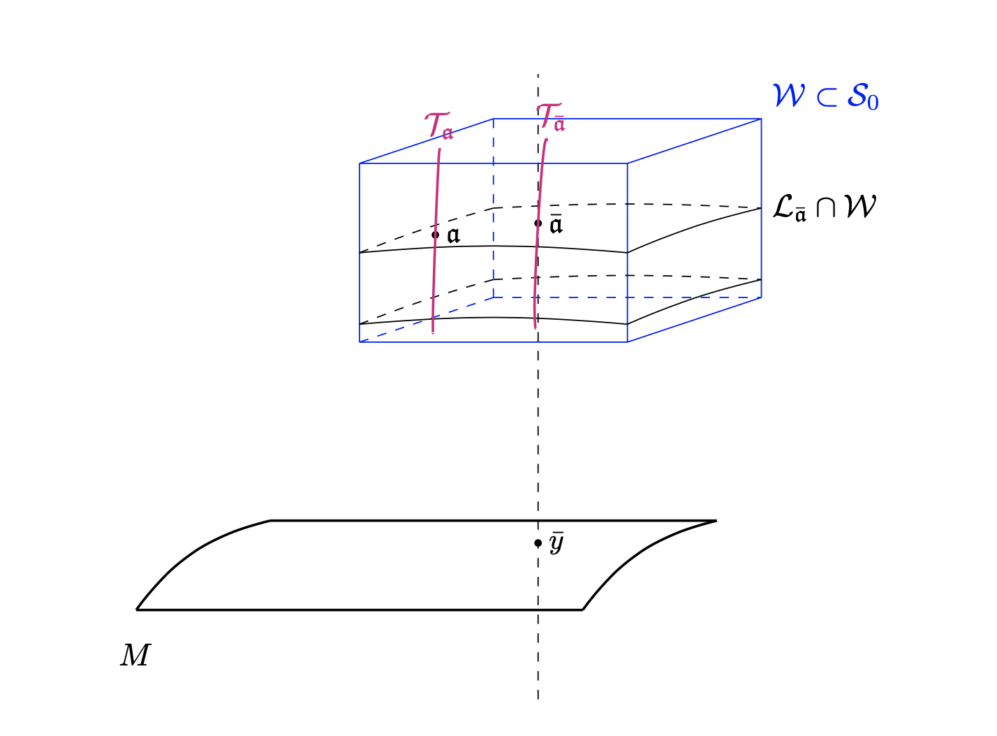
Figure 2: Local foliation chart and transverse sections

Up to shrinking $\mathcal{W}$, this family of sections allows us to define a local transition maps parametrized by the connected component of $\mathcal{L}_{\bar{{\mathfrak{a}}}}\cap\mathcal{W}$ containing $\bar{{\mathfrak{a}}}$, that is, diffeomorphisms $T^{\bar{{\mathfrak{a}}},{\mathfrak{a}}}:\mathcal{T}_{\bar{{\mathfrak{a}}}}\to\mathcal{T}_{{\mathfrak{a}}}$ for all ${\mathfrak{a}}\in\mathcal{L}_{\bar{{\mathfrak{a}}}}\cap\mathcal{W}$ defined by

$$T^{\bar{{\mathfrak{a}}},{\mathfrak{a}}}({\mathfrak{b}}):=\varphi^{-1}\Bigl{(}\left\{\varphi_{1}({\mathfrak{a}})\right\}\times\pi_{2}\left(\varphi({\mathfrak{b}})\right)\Bigr{)}\qquad\forall{\mathfrak{b}}\in\mathcal{T}_{\bar{{\mathfrak{a}}}}$$ (8.2)

Given a subset $\Gamma^{\bar{{\mathfrak{a}}}}$ of $\mathcal{T}_{\bar{{\mathfrak{a}}}}$, we will sometimes abuse notation and write

$$\Gamma^{\bar{{\mathfrak{a}}}}_{{\mathfrak{a}}}:=T^{\bar{{\mathfrak{a}}},{\mathfrak{a}}}(\Gamma^{\bar{{\mathfrak{a}}}}).$$

Transverse metric: We define a $2l$-form $\eta$ on $\Delta^{\perp}$ by

$$\eta:=\bigl{(}\omega^{\perp}\bigr{)}^{l}\quad\mbox{with}\quad l:=\frac{r}{2},$$

where $r$ is the co-rank of $\vec{\mathcal{K}}|_{\mathcal{S}_{0}}$ in respect to $\Delta^{\perp}$, that is, $r=2n-m-m_{0}$. The following lemma follows essentially from Proposition 3.2(ii) and the assumption that $\vec{\mathcal{K}}_{|S_{0}}$ is splittable, cf.$\S\S$ 7.2.

Lemma 8.2.

There are a $\vec{\mathcal{K}}$-transverse section $\mathcal{T}_{\bar{{\mathfrak{a}}}}\subset\mathcal{S}_{0}$ centered at $\bar{{\mathfrak{a}}}$ and a compact set $\tilde{\mathcal{A}}^{\bar{{\mathfrak{a}}}}\subset\mathcal{T}_{\bar{{\mathfrak{a}}}}$ such that the following properties are satisfied:

• The set $\tilde{\mathcal{A}}^{\bar{{\mathfrak{a}}}}$ has positive measure with respect to the volume form $\eta_{|\mathcal{T}_{\bar{{\mathfrak{a}}}}}$.

• For every ${\mathfrak{a}}\in\tilde{\mathcal{A}}^{\bar{{\mathfrak{a}}}}$, there is an absolutely continuous curve $\psi:[0,1]\rightarrow\Delta^{\perp}$ such that

  $$\psi(0)={\mathfrak{a}},\quad\psi(1)\in\Sigma,\quad\mbox{\em length}^{\tilde{g}}(\psi)\leq\bar{\ell}+1\quad\mbox{and}\quad\psi(t)\in\mathcal{L}_{{\mathfrak{a}}}\subset\mathcal{S}_{0}\quad\forall t\in[0,1).$$

• For any distinct points ${\mathfrak{a}},{\mathfrak{a}}^{\prime}\in\tilde{\mathcal{A}}^{\bar{{\mathfrak{a}}}}$, ${\mathfrak{a}}$ and ${\mathfrak{a}}^{\prime}$ are not $(\vec{\mathcal{K}},2\bar{\ell}+5)$-related.

Proof of Lemma 8.2.

Recall that $\bar{y}$ is a density point of $\bar{\mathcal{A}}\setminus\{\bar{x}\}$ and $\bar{{\mathfrak{a}}}\in\mathcal{S}_{0}$ satisfies $\pi(\bar{{\mathfrak{a}}})=\bar{y}$. Consider the notation of the local normal form above and for every $y\in\mathcal{U}$, denote by $\mathcal{V}_{y}$ the vertical fiber in $\Delta^{\perp}$ over $y$ given by

$$\mathcal{V}_{y}:=\pi^{-1}(\{y\})\cap T_{\bar{{\mathfrak{a}}}}\Delta^{\perp},$$

which coincides with a vector space $\vec{V}_{y}$ of dimension $n-m$ with the origin removed. Since $\vec{\mathcal{K}}(\bar{{\mathfrak{a}}})\cap T_{\bar{{\mathfrak{a}}}}\mathcal{V}_{\bar{y}}=\{0\}$ (see Theorem 1.1 (i) and (3.5)), there is a vector space $\vec{\mathcal{H}}\subset T_{\bar{{\mathfrak{a}}}}\Delta^{\perp}$ of dimension $n$ which is transverse to $T_{\bar{{\mathfrak{a}}}}\mathcal{V}_{\bar{y}}=\vec{V}_{\bar{y}}$ in $T_{\bar{{\mathfrak{a}}}}\Delta^{\perp}$, that is $\vec{\mathcal{H}}\oplus\vec{V}_{\bar{y}}=T_{\bar{{\mathfrak{a}}}}\Delta^{\perp}$, and such that $\vec{\mathcal{K}}(\bar{{\mathfrak{a}}})\subset\vec{\mathcal{H}}$. Then, we consider a vector space $\vec{\mathcal{P}}\subset\vec{\mathcal{H}}$ such that

$$\vec{\mathcal{K}}(\bar{{\mathfrak{a}}})\oplus\vec{\mathcal{P}}=\vec{\mathcal{H}}$$ (8.3)

and define the vector spaces $\vec{\mathcal{Q}}\subset T_{\bar{{\mathfrak{a}}}}\Delta^{\perp}$ and $\vec{Q},\vec{H},\vec{P}\subset\mathbb{R}^{2n-m}$ by

$$\vec{\mathcal{Q}}:=\vec{\mathcal{P}}\oplus\vec{V}_{\bar{y}},\quad\vec{Q}:=d_{\bar{{\mathfrak{a}}}}\varphi\bigl{(}\vec{\mathcal{Q}}\bigr{)},\quad\vec{H}:=d_{\bar{{\mathfrak{a}}}}\varphi\bigl{(}\vec{\mathcal{H}}\bigr{)},\quad\vec{P}:=d_{\bar{{\mathfrak{a}}}}\varphi\bigl{(}\vec{\mathcal{P}}\bigr{)}.$$

By construction, $\vec{\mathcal{H}}$ and $\vec{H}$ have dimension $n$, $\vec{\mathcal{P}}$ and $\vec{P}$ have dimension $n-m_{0}$, $\vec{\mathcal{Q}}$ and $\vec{Q}$ have dimension $r=2n-m-m_{0}$ and, remembering (8.1)-(8.3), we have

$$\vec{K}\oplus\vec{P}=\vec{H},\quad\vec{\mathcal{K}}(\bar{{\mathfrak{a}}})\oplus\vec{\mathcal{Q}}=T_{\bar{{\mathfrak{a}}}}\Delta^{\perp},\quad\vec{K}\oplus\vec{Q}=\mathbb{R}^{2n-m}.$$ (8.4)

Then, we define two $n$-dimensional open smooth manifolds $H\subset W$ and $\mathcal{H}\subset\mathcal{W}$ by

$$H:=\vec{H}\cap W\quad\mbox{and}\quad\mathcal{H}:=\varphi^{-1}(H),$$

and note that the restriction of $\pi$ to $\mathcal{H}$ is a submersion at $\bar{{\mathfrak{a}}}$. Therefore, there is a smooth submanifold $I$ of $W$ of dimension $n$ containing $\bar{a}=0$ of the form ($|\cdot|$ stands for the Euclidean norm in $\mathbb{R}^{m_{0}}$ or $\mathbb{R}^{2n-m}$)

$$I=\left\{(a_{1},0)+p\,|\,a_{1}\in W^{1},\,p\in\vec{P},\,|a_{1}|^{2}+|p|^{2}<\delta^{2}\right\}\subset H,$$

with $\delta>0$, such that the mapping

$$F=\pi_{|\mathcal{I}}\,:\,\mathcal{I}:=\varphi^{-1}(I)\,\longrightarrow\,\mathcal{E}:=\pi(\mathcal{I})$$

is a smooth diffeomorphism. Then, we denote by $\bar{W}^{1}$ the set of $a_{1}\in W^{1}$ with $|a_{1}|\leq\delta/2$ and for each $a_{1}\in\bar{W}_{1}$, we define the sets $P_{a_{1}}\subset H$, $\mathcal{P}_{a_{1}}\subset\mathcal{H}$, $\mathcal{E}_{a_{1}}\subset\mathcal{E}$, $\mathcal{Q}_{a_{1}}\subset\mathcal{W}$ and $Q_{a_{1}}\subset W$ by

$$P_{a_{1}}:=\bigl{(}(a_{1},0)+\vec{P}\bigr{)}\cap I,\quad\mathcal{P}_{a_{1}}:=\varphi^{-1}\left(P_{a_{1}}\right),\quad\mathcal{E}_{a_{1}}:=F\left(\mathcal{P}_{a_{1}}\right).$$

$$\mathcal{Q}_{a_{1}}:=\left\{(y,q)+(0,h)\,|\,(y,q)\in\mathcal{P}_{a_{1}},\,h\in\vec{V}_{y},\,|h|<\delta\right\}\quad\mbox{and}\quad Q_{a_{1}}:=\varphi\left(\mathcal{Q}_{a_{1}}\right).$$

By construction, for each $a_{1}\in\bar{W}^{1}$, the set $P_{a_{1}}$ is an open smooth submanifold of $W$ of dimension $n-m_{0}$, the set $\mathcal{P}_{a_{1}}$ is an open smooth submanifold of $\mathcal{W}$ of dimension $n-m_{0}$ and the set $\mathcal{E}_{a_{1}}$ is an open smooth submanifold of $\mathcal{U}$ of dimension $n-m_{0}$. Moreover, since by $\vec{\mathcal{P}}\cap\vec{V}_{\bar{y}}=d_{0}\varphi^{-1}(\vec{P})\cap T_{\bar{{\mathfrak{a}}}}\mathcal{V}_{\bar{y}}=\{0\}$ the mapping

$$({\mathfrak{a}},h)\in\left\{((y,q),h)\,|\,(y,q)\in\mathcal{P}_{0},\,h\in\vec{V}_{y}\right\}\,\longmapsto\,{\mathfrak{a}}+(0,h)\in\Delta^{\perp}$$

is an immersion at $(\bar{{\mathfrak{a}}},0)$ valued in $\mathcal{Q}_{0}$ and since the mapping

$$a\in\vec{Q}\,\longmapsto\bigl{(}0,\pi^{2}(a)\bigr{)}\in T_{0}\bigl{(}\{0\}\times W^{2}\bigr{)}$$

is a linear isomorphism (by (8.4) we have $\vec{K}\oplus\vec{Q}=\mathbb{R}^{2n-m}$), we may assume by taking $\delta>0$ small enough for each $a_{1}\in\bar{W}^{1}$, that the sets $\mathcal{Q}_{a_{1}}$ and $Q_{a_{1}}$ are open smooth manifolds of dimension $r$ and that the mapping

$$G_{a_{1}}\,:\,a\in Q_{a_{1}}\,\longmapsto\,\bigl{(}0,\pi^{2}(a)\bigr{)}\in T_{0}\bigl{(}\{0\}\times W^{2}\bigr{)}$$

is a smooth diffeomorphism from $Q_{a_{1}}$ onto its image $G_{a_{1}}(Q_{a_{1}})$. By the way, we notice that for every $a_{1}\in\bar{W}^{1}$ and every $a\in Q_{a_{1}}$, the two points $a$ and $b=G_{a_{1}}(a)$ have the same coordinate in $W^{2}$ so that their images by $\varphi^{-1}$, $\varphi^{-1}(a)$ and $\varphi^{-1}(b)$, belong to the same plaque and to the same leaf of the foliation defined by $\vec{\mathcal{K}}$ in $\mathcal{W}$. So, by the construction made before the statement of the lemma, the points $\varphi^{-1}(a)\in\mathcal{W}$ and $\varphi^{-1}(b)\in\mathcal{T}_{\bar{{\mathfrak{a}}}}$ can be connected through a smooth curve horizontal with respect to $\vec{\mathcal{K}}$ of length (w.r.t $\tilde{g}$) less than 1. We are now ready to conclude the proof of the Lemma.

By construction, the sets $P_{a_{1}}$ as well as $\mathcal{P}_{a_{1}}$, $\mathcal{E}_{a_{1}}$, with $a_{1}\in\bar{W}^{1}$ are pairwise disjoint and satisfy

$$\bigcup_{a_{1}\in\bar{W}^{1}}P_{a_{1}}=I\quad\bigcup_{a_{1}\in\bar{W}^{1}}\mathcal{P}_{a_{1}}=\mathcal{I},\quad\bigcup_{a_{1}\in\bar{W}^{1}}\mathcal{E}_{a_{1}}=\mathcal{E}.$$

Since $\bar{y}$ is a density point of $\bar{\mathcal{A}}$, by Fubini’s Theorem, we infer that there is $\tilde{a}_{1}\in\bar{W}^{1}$ such that the $(n-m_{0})$-dimensional Lebesgue measure of the set

$$\Theta:=\bar{\mathcal{A}}\cap\bar{\mathcal{E}}_{\tilde{a}_{1}}\subset\bar{\mathcal{E}}_{\tilde{a}_{1}}$$

is positive. In fact, by taking a compact subset of $\Theta$ of positive measure, we may indeed assume that $\Theta$ is compact. By construction, for every $\theta\in\Theta$, there is an horizontal path $\gamma^{\theta}\in\Omega_{\Delta}^{\bar{x}}$ of length $\leq\bar{\ell}$ (w.r.t $g$) such that $\gamma^{\theta}(1)=\theta$, $\mbox{rank}^{\Delta}(\gamma)=m$ and for which all abnormal lifts meet the set $\Sigma$. Hence, by Proposition 3.4, for every $p\in\Delta^{\perp}_{\theta}$, $\gamma^{\theta}$ admits an abnormal lift $\psi^{\theta,p}:[0,1]\rightarrow\Delta^{\perp}$ such that $\psi^{\theta,p}(1)=(\theta,p)$ and $\psi^{x,p}([0,1])\cap\Sigma\neq\emptyset$. Thus, we obtain that any ${\mathfrak{a}}$ in the set

$$\tilde{\Theta}:=\left\{F^{-1}(\theta)+(0,h)\,|\,\theta\in\Theta,\,h\in\vec{V}_{\theta},\,|h|\leq\delta\right\}$$

can be joined to $\Sigma$ by a curve of length $\leq\bar{\ell}$. By Fubini’s Theorem, the set $\tilde{\Theta}$ is a compact set of positive measure in the manifold $\mathcal{Q}_{\tilde{a_{1}}}$, thus its image by $\varphi$, $\varphi(\tilde{\Theta})$, is a compact set of positive measure in the manifold $Q_{\tilde{a_{1}}}$, the image of $\varphi(\tilde{\Theta})$ by $G_{\tilde{a}_{1}}$, $\Lambda:=(G_{\tilde{a}_{1}}\circ\varphi)(\tilde{\Theta})$ has positive measure in $\{0\}\times W^{2}$ and the image of $\Lambda$ by $\varphi^{-1}$ has positive measure in $\mathcal{T}_{\bar{{\mathfrak{a}}}}$. By construction, any point of $\varphi^{-1}(\Lambda)$ can be joined to a point of $\Sigma$ by an absolutely continuous curve horizontal with respect to $\vec{\mathcal{K}}$ of length (w.r.t $\tilde{g}$) $\leq\bar{l}+1$. By assumption of splittability, we can select in $\varphi^{-1}(\Lambda)$ a compact subset $\tilde{\mathcal{A}}^{\bar{{\mathfrak{a}}}}$ of positive measure satisfying the same property and whose points are not $(\vec{\mathcal{K}},2\bar{\ell}+5)$-related. Proposition 3.2 (ii) completes the proof. ∎

The next result combines the geometrical framework of Lemma 8.2 with a compactness argument and the witness section given by Theorem 7.1.

Lemma 8.3.

There are a point $\hat{{\mathfrak{a}}}\in\Sigma$, a compact set $\check{\mathcal{A}}^{\bar{{\mathfrak{a}}}}\subset\tilde{\mathcal{A}}^{\bar{{\mathfrak{a}}}}\subset\mathcal{T}_{\bar{{\mathfrak{a}}}}$, a relatively compact open neighborhood $V\subset\Delta^{\perp}$ of $\hat{{\mathfrak{a}}}$, a compact set $\check{\Sigma}\subset\Sigma\cap V$, a real analytic function $h:V\to[0,\infty)$, a semi-analytic set $X\subset V\setminus\Sigma$ and $C,\nu,\epsilon>0$ such that the following properties are satisfied:

• The set $h^{-1}(0)$ is equal to $\Sigma\cap V$.

• For every $0<c<\epsilon$, the semi-analytic set $X^{c}:=X\cap h^{-1}(c)$ has $r$-dimensional volume with respect to $\tilde{g}$ bounded by $C$. In particular, $X^{c}$ is a $r$-dimensional set and $X$ is a $(r+1)$-dimensional set.

• For every $0<c<\epsilon$ and for every ${\mathfrak{a}}\in h^{-1}(c)\subset V\setminus\Sigma$, there is a smooth curve $\alpha:[0,1]\rightarrow V\setminus\Sigma$ which is contained in $\mathcal{L}_{{\mathfrak{a}}}\cap h^{-1}(c)$ such that

  $$\alpha(0)={\mathfrak{a}},\quad\alpha(1)\in X^{c},\quad\mbox{and}\quad\mbox{\em length}^{\tilde{g}}(\alpha)\leq 1.$$

• For every $0<c<\epsilon$, we can decompose $X^{c}$ as the union of two disjoint semi-analytic sets $Y^{c}$ and $Z^{c}$, such that $Z^{c}$ has dimension $<r$, and $Y^{c}$ is the union of finitely many smooth semi-analytic sets $Y_{i}^{c}$, with $i\in I^{c}$, of dimension $r$ such that

  $$\partial Y^{c}=\overline{Y^{c}}\setminus Y^{c}\subset Z^{c}\quad\text{ and }\quad T_{{\mathfrak{a}}}\Delta^{\perp}=T_{{\mathfrak{a}}}Y_{i}^{c}+\vec{\mathcal{K}}({\mathfrak{a}})\qquad\forall{\mathfrak{a}}\in Y_{i}^{c},\,\forall i\in I_{c}.$$

• For all ${\mathfrak{a}}\in\check{\mathcal{A}}^{\bar{{\mathfrak{a}}}}$, there is an absolutely continuous curve $\psi:[0,1]\rightarrow\Delta^{\perp}$ such that

  $$\psi(0)={\mathfrak{a}},\quad\psi(1)\in\check{\Sigma},\quad\mbox{\em length}^{\tilde{g}}(\psi)\leq\bar{\ell}+1\quad\mbox{and}\quad\psi(t)\in\mathcal{L}_{{\mathfrak{a}}}\subset\mathcal{S}_{0}\quad\forall t\in[0,1).$$

• The set $\check{\mathcal{A}}^{\bar{{\mathfrak{a}}}}$ has measure $\geq\nu$ with respect to the volume form $\eta_{|\mathcal{T}_{\bar{{\mathfrak{a}}}}}$.

Moreover, there is a continuous function $\delta:[0,\infty)\rightarrow[0,\infty)$ with $\delta(0)=0$ such that for every $0<c<\epsilon$ and every ${\mathfrak{a}}\in h^{-1}(c)$,

$$\left|\eta_{{\mathfrak{a}}}\left(\xi_{1},\ldots,\xi_{d}\right)\right|\leq\delta(c)|\xi_{1}|^{\tilde{g}}\cdots|\xi_{d}|^{\tilde{g}}\qquad\forall\xi_{1},\ldots,\xi_{d}\in T_{{\mathfrak{a}}}\Delta^{\perp}.$$ (8.5)

Proof of Lemma 8.3.

Let $N:=\Delta^{\perp}$ be the real-analytic manifold of dimension $2n-m$ equipped with the singular analytic foliation $\vec{\mathcal{F}}$ of generic corank $r=2n-m-m_{0}$ with singular set $\Sigma$ and $\mathcal{B}\subset\Sigma$ the set of ${\mathfrak{a}}\in\Sigma$ for which there is an absolutely continuous curve $\psi:[0,1]\rightarrow\Delta^{\perp}$ such that

$$\psi(0)\in\tilde{\mathcal{A}}^{\bar{{\mathfrak{a}}}},\quad\psi(1)={\mathfrak{a}},\quad\mbox{length}^{\tilde{g}}(\psi)\leq\bar{\ell}+1\quad\mbox{and}\quad\psi(t)\in\mathcal{L}_{\psi(0)}\subset\mathcal{S}_{0}\quad\forall t\in[0,1),$$

where $\tilde{\mathcal{A}}^{\bar{{\mathfrak{a}}}}\subset\mathcal{T}_{\bar{{\mathfrak{a}}}}$ is the set provided by Lemma 8.2. The compactness of $\tilde{\mathcal{A}}^{\bar{{\mathfrak{a}}}}$ together with the closedness of $\Sigma$ and the upper bound on the length of curves (with the completeness of $\tilde{g}$) imply that $\mathcal{B}$ is a compact subset of $\Sigma$. By Theorem 7.1 applied with $\ell=1$, for every ${\mathfrak{a}}\in\mathcal{B}$, there are a relatively compact open neighborhood $V_{{\mathfrak{a}}}$ of ${\mathfrak{a}}$ in $N=\Delta^{\perp}$, a real-analytic function $h_{{\mathfrak{a}}}:V_{{\mathfrak{a}}}\to[0,\infty)$, a semi-analytic set $X_{{\mathfrak{a}}}\subset V_{{\mathfrak{a}}}\setminus\Sigma$ and $C_{{\mathfrak{a}}}>0$ such that the properties (i)-(iv) of Theorem 7.1 are satisfied. Pick for each ${\mathfrak{a}}\in\mathcal{B}$ a compact neighborhood $\check{V}_{{\mathfrak{a}}}\subset V_{{\mathfrak{a}}}$ of ${\mathfrak{a}}$ and consider by compactness of $\mathcal{B}$ a finite family $\{{\mathfrak{a}}_{i}\}_{i\in I}$ such that

$$\mathcal{B}\subset\bigcup_{i\in I}\check{V}_{{\mathfrak{a}}_{i}}\subset\bigcup_{i\in I}V_{{\mathfrak{a}}_{i}}.$$ (8.6)

Then, for every $i\in I$, denote by $\tilde{\mathcal{A}}_{i}^{\bar{{\mathfrak{a}}}}$ the set of ${\mathfrak{a}}\in\tilde{\mathcal{A}}^{\bar{{\mathfrak{a}}}}$ for which there is an absolutely continuous curve $\psi:[0,1]\rightarrow\Delta^{\perp}$ such that

$$\psi(0)={\mathfrak{a}},\quad\psi(1)\in\check{\Sigma}_{i},\quad\mbox{length}^{\tilde{g}}(\psi)\leq\bar{\ell}+1\quad\mbox{and}\quad\psi(t)\in\mathcal{L}_{{\mathfrak{a}}}\subset\mathcal{S}_{0}\quad\forall t\in[0,1),$$

with $\check{\Sigma}_{i}:=\Sigma\cap\check{V}_{{\mathfrak{a}}_{i}}\cap\mathcal{B}$. We claim that each set $\mathcal{A}_{i}^{\bar{{\mathfrak{a}}}}$ is a Borel subset of $\tilde{\mathcal{A}}^{\bar{{\mathfrak{a}}}}$. As a matter of fact, for each $i\in I$, we can write

$$\mathcal{A}_{i}^{\bar{{\mathfrak{a}}}}=\bigcap_{k\in\mathbb{N}^{*}}\mathcal{A}_{i,k}^{\bar{{\mathfrak{a}}}},$$

where for each $k\in\mathbb{N}^{*}$, the set $\mathcal{A}_{i,k}^{\bar{{\mathfrak{a}}}}$ is defined as the set of ${\mathfrak{a}}\in\tilde{\mathcal{A}}^{\bar{{\mathfrak{a}}}}$ for which there is an absolutely continuous curve $\psi:[0,1]\rightarrow\mathcal{L}_{{\mathfrak{a}}}\in\mathcal{S}_{0}$ such that

$$\psi(0)={\mathfrak{a}},\quad\psi(1)\in B_{1/k}^{\tilde{g}}\left(\check{\Sigma}_{i}\right)\cap\left(V\setminus\Sigma\right),\quad\mbox{length}^{\tilde{g}}(\psi)<\bar{\ell}+1,$$

with

$$B_{1/k}^{\tilde{g}}\left(\check{\Sigma}_{i}\right):=\left\{{\mathfrak{a}}^{\prime}\in\Delta^{\perp}\,|\,d^{\tilde{g}}\left({\mathfrak{a}}^{\prime},\check{\Sigma}_{i}\right)<\frac{1}{k}\right\}.$$

By regularity of $\vec{\mathcal{K}}_{|\mathcal{S}_{0}}$, each set $\mathcal{A}_{i,k}^{\bar{{\mathfrak{a}}}}$ is open in $\tilde{\mathcal{A}}^{\bar{{\mathfrak{a}}}}$, so we infer that each $\mathcal{A}_{i}^{\bar{{\mathfrak{a}}}}$ is a Borel subset of $\tilde{\mathcal{A}}^{\bar{{\mathfrak{a}}}}$. Furthermore, by construction of $\mathcal{B}$, (8.6) and Lemma 8.2 (ii), we have

$$\tilde{\mathcal{A}}^{\bar{{\mathfrak{a}}}}=\bigcup_{i\in I}\tilde{\mathcal{A}}_{i}^{\bar{{\mathfrak{a}}}}.$$

As a consequence, since $\tilde{\mathcal{A}}^{\bar{{\mathfrak{a}}}}$ has positive measure with respect to the volume form $\eta_{|\mathcal{T}_{\bar{{\mathfrak{a}}}}}$ (Lemma 8.2 (i)), there is $i\in I$ such that $\tilde{\mathcal{A}}^{\bar{{\mathfrak{a}}}}_{i}$ and a compact subset $\check{\mathcal{A}}^{\bar{{\mathfrak{a}}}}_{i}$ of it satisfy the same property. We conclude the proof of (i)-(vi) by setting $\check{\mathcal{A}}^{\bar{{\mathfrak{a}}}}:=\check{\mathcal{A}}^{\bar{{\mathfrak{a}}}}_{i}$, $V:=V_{{\mathfrak{a}}_{i}}$, $\check{\Sigma}:=\check{\Sigma}_{i}$, $h:=h_{{\mathfrak{a}}_{i}}$, $X:=X_{{\mathfrak{a}}_{i}}$, $C:=C_{{\mathfrak{a}}_{i}}$ and $\nu$ the volume of $\check{\mathcal{A}}^{\bar{{\mathfrak{a}}}}$ with respect to $\eta_{|\mathcal{T}_{\bar{{\mathfrak{a}}}}}$.

The second part of the proof (8.5) follows from Proposition 3.2 (ii). By Theorem 1.1 (iv), we have

$$\dim\left(\mbox{ker}\bigl{(}\omega^{\perp}_{{\mathfrak{a}}}\bigr{)}\right)\geq m_{0}+2\qquad\forall{\mathfrak{a}}\in\Sigma.$$

Therefore, by Proposition 3.2 (iii), we have $\eta_{{\mathfrak{a}}}=0$ for all ${\mathfrak{a}}\in\check{\Sigma}$ and we can conclude by regularity of $h$ near the compact set $\check{\Sigma}\subset V$. ∎

The idea of our proof consists now in obtaining a contradiction from the construction of an homotopy sending smoothly the points of a small neighborhood of a set $\check{\mathcal{A}}^{\bar{{\mathfrak{a}}},c}\subset\check{\mathcal{A}}^{\bar{{\mathfrak{a}}}}$ in $\mathcal{T}_{\bar{{\mathfrak{a}}}}$ to an open subset of $Y^{c}$ for $c>0$ small enough. Since this homotopy has to preserve the leaves of $\vec{\mathcal{K}}_{|\mathcal{S}_{0}}$, we perform the construction by following the minimizing geodesics from $\mathcal{T}_{\bar{{\mathfrak{a}}}}$ to $Y^{c}$ with respect to some complete metric on $\mathcal{S}_{0}$ that needs to be built (note that $\tilde{g}$ is not complete when restricted to $\mathcal{S}_{0}$). The next Lemma formalizes this framework:

Lemma 8.4.

For every $0<c<\epsilon$, there are a smooth Riemannian metric $\tilde{g}^{c}$ on $\mathcal{S}_{0}$ and a compact set $\check{\mathcal{A}}^{\bar{{\mathfrak{a}}},c}\subset\check{\mathcal{A}}^{\bar{{\mathfrak{a}}}}$ satisfying the following properties:

• The Riemannian manifold $(\mathcal{S}_{0},\tilde{g}^{c})$ is complete.

• For every ${\mathfrak{a}}\in\check{\mathcal{A}}^{\bar{{\mathfrak{a}}},c}$, there is an absolutely continuous curve $\psi:[0,1]\rightarrow\mathcal{L}_{{\mathfrak{a}}}\subset\mathcal{S}_{0}$ such that (where $Y^{c}$ is defined in Lemma 8.3(iv))

  $$\psi(0)={\mathfrak{a}},\quad\psi(1)\in Y^{c}\quad\mbox{and}\quad\mbox{\em length}^{\tilde{g}}(\psi)=\mbox{\em length}^{\tilde{g}^{c}}(\psi)<\bar{\ell}+2.$$

• The set $\check{\mathcal{A}}^{\bar{{\mathfrak{a}}},c}$ has measure $\geq\nu/4$ with respect to the volume form $\eta_{|\mathcal{T}_{\bar{{\mathfrak{a}}}}}$.

• Let $\mathcal{C}^{c}\subset\mathcal{S}_{0}$ be the set of points ${\mathfrak{a}}\in\mathcal{S}_{0}$ for which there is an absolutely continuous curve $\psi:[0,1]\rightarrow\mathcal{L}_{{\mathfrak{a}}}$ of length $\leq\bar{\ell}+2$ with respect to $\tilde{g}^{c}$ joining ${\mathfrak{a}}$ to a point of $\overline{Z^{c}}$ (defined in Lemma 8.3(iv)). Then $\mathcal{C}^{c}$ is closed and does not intersect $\check{\mathcal{A}}^{\bar{{\mathfrak{a}}},c}$.

Proof of Lemma 8.4.

Since $\Sigma$ is a closed subset of $\Delta^{\perp}$, we can pick a smooth function $F:\Delta^{\perp}\rightarrow[0,\infty)$ such that

$$\Sigma=F^{-1}\left(\{0\}\right)$$

and fix some $c>0$. Consider the function $D:\mathbb{R}^{+}\rightarrow[0,+\infty]$ given by

$$D(\lambda):=\left\{\begin{array}[]{rcl}\frac{1}{\bar{\ell}+2-\lambda}&\mbox{ if }&\lambda<\bar{\ell}+2\\ +\infty&\mbox{ if }&\lambda\geq\bar{\ell}+2\end{array}\right.\qquad\forall\lambda\in\mathbb{R}^{+}$$

and define the function $\Psi^{c}:\mathcal{T}_{\bar{{\mathfrak{a}}}}\rightarrow[0,\infty]$ by

$$\Psi^{c}({\mathfrak{a}}):=\inf\Bigl{\{}D\left(\mbox{length}^{\tilde{g}}(\psi)\right)+\max\left(F\bigl{(}\psi([0,1])\bigr{)}^{-1}\right)\,|\,\psi\in\Omega\left({\mathfrak{a}},\overline{X^{c}}\right)\Bigr{\}}$$

where for every ${\mathfrak{a}}\in\mathcal{T}_{\bar{{\mathfrak{a}}}}$, $\Omega\left({\mathfrak{a}},\overline{X^{c}}\right)$ stands for the set of absolutely continuous curves $\psi:[0,1]\rightarrow\mathcal{S}_{0}$ such that $\psi(0)={\mathfrak{a}}$, $\psi(1)\in\overline{X^{c}}$ and $\psi$ is almost everywhere tangent to $\vec{\mathcal{K}}_{|\mathcal{S}_{0}}$. Let ${\mathfrak{a}}\in\check{\mathcal{A}}^{\bar{{\mathfrak{a}}}}$ be fixed, by Lemma 8.3 (v), there is an absolutely continuous curve $\psi:[0,1]\rightarrow\Delta^{\perp}$ such that $\psi(0)={\mathfrak{a}}$, $\psi(1)\in\check{\Sigma}$, $\mbox{length}^{\tilde{g}}(\psi)\leq\bar{\ell}+1$ and $\psi(t)\in\mathcal{L}_{{\mathfrak{a}}}\subset\mathcal{S}_{0}$ for all $t\in[0,1)$. Thus, since $\psi(t)$ belongs to $V\setminus\Sigma$ for $t$ close to $1$, Lemma 8.3(iii) shows that ${\mathfrak{a}}$ can be joined to $Xc$ by a curve tangent to $\mathcal{L}_{{\mathfrak{a}}}$ contained in $\mathcal{S}_{0}$ of length $<\bar{\ell}+2$. Therefore $\Psi^{c}({\mathfrak{a}})$ is finite for every ${\mathfrak{a}}\in\check{\mathcal{A}}^{\bar{{\mathfrak{a}}}}$. Moreover, the function $\Psi^{c}$ is lower semi-continuous on $\mathcal{T}_{\bar{{\mathfrak{a}}}}$ (because we consider curves satisfying $\psi(1)\in\overline{X^{c}}$ and we may use foliation charts along $\psi$), so we have

$$\check{\mathcal{A}}^{\bar{{\mathfrak{a}}}}=\bigcup_{k\in\mathbb{N}}\check{\mathcal{A}}^{\bar{{\mathfrak{a}}}}_{k}\quad\mbox{with}\quad\check{\mathcal{A}}^{\bar{{\mathfrak{a}}}}_{k}:=\left(\Psi^{c}\right)^{-1}\bigl{(}[0,k]\bigr{)}\cap\check{\mathcal{A}}^{\bar{{\mathfrak{a}}}},$$

where each set of the above union is a compact subset of $\check{\mathcal{A}}^{\bar{{\mathfrak{a}}}}$. Thus, there is $k\in\mathbb{N}$ such that the measure of $\check{\mathcal{A}}^{\bar{{\mathfrak{a}}}}_{k}$ with respect to the volume form $\eta_{|\mathcal{T}_{\bar{{\mathfrak{a}}}}}$ is $\geq\nu/2$ and such that for every ${\mathfrak{a}}\in\check{\mathcal{A}}^{\bar{{\mathfrak{a}}}}_{k}$, there is an absolutely continuous curve $\psi:[0,1]\rightarrow\mathcal{L}_{{\mathfrak{a}}}\subset\mathcal{S}_{0}$ satisfying $\psi(0)={\mathfrak{a}}$, $\psi(1)\in\overline{X^{c}}$ and

$$D\left(\mbox{length}^{\tilde{g}}(\psi)\right)+\max\left(F\bigl{(}\psi([0,1])\bigr{)}^{-1}\right)\leq k,$$

which implies

$$\mbox{length}^{\tilde{g}}(\psi)<\bar{\ell}+2\quad\mbox{and}\quad\min\left(F\bigl{(}\psi([0,1])\bigr{)}\right)\geq\frac{1}{k}.$$

Fix a smooth complete metric $\tilde{g}^{c}$ on $\mathcal{S}_{0}$ which coincides with $\tilde{g}$ on the set $F^{-1}([1/(k),\infty))$. Recall that the definition of $Y^{c}$ and $Z^{c}$ is given in Lemma 8.3(iv), and note that $\overline{X^{c}}=\overline{Y^{c}}\cup\overline{Z^{c}}$, where $\overline{Z^{c}}$ has dimension $\leq r-1$. By Lemma 8.3 (iv), the boundary $\partial Y^{c}:=\overline{Y^{c}}\setminus Y^{c}$ is contained in $Z^{c}$, so the set of points of $\mathcal{S}_{0}$ that can be joined to $\overline{Z^{c}}$ along absolutely continuous curves tangent to $\vec{\mathcal{K}}_{|\mathcal{S}_{0}}$ is a countable union of smooth submanifolds of dimension at most $r-1+m_{0}=2n-m-1$, so it has measure zero in $\mathcal{S}_{0}$ and in fact since it is invariant by the foliation associated with $\vec{\mathcal{K}}_{|\mathcal{S}_{0}}$, its intersection with $\mathcal{T}_{\bar{{\mathfrak{a}}}}$ has measure zero in $\mathcal{T}_{\bar{{\mathfrak{a}}}}$ (by Fubini’s Theorem). Thus, we can consider a compact subset $\check{\mathcal{A}}^{\bar{{\mathfrak{a}}},c}$ of $\check{\mathcal{A}}^{\bar{{\mathfrak{a}}}}_{k}\subset\check{\mathcal{A}}^{\bar{{\mathfrak{a}}}}$ of measure $\geq\nu/4$ such that the properties (i)-(iii) are satisfied. Finally, the set $\mathcal{C}^{c}$ is closed because $\partial Y^{c}$ is closed and $(\mathcal{S}_{0},\tilde{g}^{c})$ is complete. We conclude that $\check{\mathcal{A}}^{\bar{{\mathfrak{a}}},c}$ satisfies (iv) by construction. ∎

Given $0<c<\epsilon$, we define the function $D^{c}:\mathcal{S}_{0}\setminus\mathcal{C}^{c}\rightarrow[0,\infty]$ by

$$D^{c}({\mathfrak{a}}):=\inf\Bigl{\{}\mbox{length}^{\tilde{g}^{c}}(\psi)\,|\,\psi:[0,1]\rightarrow\mathcal{L}_{{\mathfrak{a}}}\mbox{ abs. cont. }\,\psi(0)={\mathfrak{a}},\,\psi(1)\in Y^{c}\Bigr{\}},$$

for every ${\mathfrak{a}}\in\mathcal{S}_{0}\setminus\mathcal{C}^{c}$, and we denote its domain, the set of points ${\mathfrak{a}}\in\mathcal{S}_{0}\setminus C^{c}$, where $D^{c}({\mathfrak{a}})$ is finite, by $\mbox{dom}(D^{c})$. Then, we call $\mathcal{L}_{{\mathfrak{a}}}$-geodesic a curve $\psi:[0,1]\rightarrow\mathcal{L}_{{\mathfrak{a}}}$ which is geodesic with respect to the metric $\tilde{g}^{c,{\mathfrak{a}}}$ induced by $\tilde{g}^{c}$ on $\mathcal{L}_{{\mathfrak{a}}}$, for any point ${\mathfrak{a}}\in Y^{c}$ we denote by $\exp_{{\mathfrak{a}}}^{c}:T_{{\mathfrak{a}}}\mathcal{L}_{{\mathfrak{a}}}\rightarrow\mathcal{L}_{{\mathfrak{a}}}$ the exponential map from ${\mathfrak{a}}$ with respect to $\tilde{g}^{c,{\mathfrak{a}}}$ and by considering $\vec{\mathcal{K}}_{Y^{c}}$ as a subbundle of $T\Delta^{\perp}$ (that is, for every ${\mathfrak{a}}\in Y^{c}$ we take $\vec{\mathcal{K}}({\mathfrak{a}})$) we define the smooth mapping $\mbox{Exp}^{c}:\vec{\mathcal{K}}_{Y^{c}}\rightarrow\mathcal{S}_{0}$ by

$$\mbox{Exp}^{c}({\mathfrak{a}},\zeta):=\exp_{{\mathfrak{a}}}^{c}(\zeta)\qquad\forall({\mathfrak{a}},\zeta)\in\vec{\mathcal{K}}_{Y^{c}}.$$

By completeness of $(\mathcal{S}_{0},\tilde{g}^{c})$, see Lemma 8.4 (i), for every ${\mathfrak{a}}\in\mbox{dom}(D^{c})$ any sequence $\{\psi_{k}:[0,1]\rightarrow\mathcal{L}_{{\mathfrak{a}}}\}_{k\in\mathbb{N}}$ of absolutely continuous curves such that

$$\psi_{k}(0)={\mathfrak{a}},\quad\psi_{k}(1)\in Y^{c}\quad\mbox{and}\quad\lim_{k\rightarrow\infty}\mbox{length}^{g^{c}}(\psi_{k})=D^{c}({\mathfrak{a}}),$$

converges, up to taking a subsequence, to a $\mathcal{L}_{{\mathfrak{a}}}$-geodesic $\bar{\psi}$, called minimizing geodesic for $D^{c}({\mathfrak{a}})$, satisfying $\bar{\psi}(0)={\mathfrak{a}}$, $\bar{\psi}(1)\in\overline{Y^{c}}$ and $\mbox{length}^{g^{c}}(\psi_{k})=D^{c}({\mathfrak{a}})$. Moreover if in addition $D^{c}({\mathfrak{a}})<\bar{l}+2$ then we have $\bar{\psi}(1)\in Y^{c}$ because ${\mathfrak{a}}\in\mbox{dom}(D^{c})\subset\mathcal{S}_{0}\setminus\mathcal{C}^{c}$. For every ${\mathfrak{a}}\in\mbox{dom}(D^{c})$, we set

$$\Gamma^{c}({\mathfrak{a}}) \quad\text{the set of all minimizing geodesics for}\,D^{c}({\mathfrak{a}}),$$ (8.7)

$$\mathcal{I}^{c}({\mathfrak{a}}) :=\Bigl{\{}\psi(t)\,|\,\psi\in\Gamma^{c}({\mathfrak{a}}),\,t\in[0,1]\Bigr{\}}.$$

By completeness of $(\mathcal{S}_{0},\tilde{g}^{c})$ and regularity of the foliation given by $\vec{\mathcal{K}}_{|\mathcal{S}_{0}}$, the mapping ${\mathfrak{a}}\in\mbox{dom}(D^{c})\mapsto\mathcal{I}^{c}({\mathfrak{a}})$ has closed graph. Moreover, by the above construction and properties (iii)-(iv) of Lemma 8.4, the set

$$\mathcal{I}^{c}\left(\check{\mathcal{A}}^{\bar{{\mathfrak{a}}},c}\right):=\bigcup_{{\mathfrak{a}}\in\check{\mathcal{A}}^{\bar{{\mathfrak{a}}},c}}\mathcal{I}^{c}({\mathfrak{a}})$$

is a compact subset of $\mathcal{S}_{0}$ which is contained in $\mbox{dom}(D^{c})$. The following lemma follows from classical results on distance functions from submanifolds in Riemannian geometry (see Figure 3).

Lemma 8.5.

For every $0<c<\epsilon$, there are an open subset $\mathcal{V}^{c,\bar{{\mathfrak{a}}}}$ of $\mathcal{T}_{\bar{{\mathfrak{a}}}}$ containing $\check{\mathcal{A}}^{\bar{{\mathfrak{a}}},c}$, an open neighborhood $\mathcal{H}^{c}$ of $\bar{{\mathfrak{a}}}$ in $\mathcal{L}_{\bar{{\mathfrak{a}}}}$, an open set $\mathcal{U}^{c}\subset\mathcal{W}$ and a set $F^{c}\subset\mathcal{U}^{c}$ satisfying the following properties:

• The set $F^{c}\subset\mathcal{U}^{c}$ is closed with respect to the induced topology on $\mathcal{U}^{c}$.

• The set $F^{c}$ has Lebesgue measure zero in $\mathcal{U}^{c}$.

• The function $D^{c}$ is smooth on the open set (recall the notation introduced for local transition maps (8.2))

  $$\mathcal{U}^{c}\setminus F^{c}\quad\mbox{with}\quad\mathcal{U}^{c}:=\bigcup_{{\mathfrak{a}}\in\mathcal{H}^{c}}T^{\bar{{\mathfrak{a}}},{\mathfrak{a}}}(\mathcal{V}^{c,\bar{{\mathfrak{a}}}})=\bigcup_{{\mathfrak{a}}\in\mathcal{H}^{c}}\mathcal{V}^{c,\bar{{\mathfrak{a}}}}_{{\mathfrak{a}}}\subset\mathcal{W}$$

  and for every ${\mathfrak{a}}\in\mathcal{U}^{c}\setminus F^{c}$ the set $\Gamma^{c}({\mathfrak{a}})$ given in (8.7) is a singleton $\{\psi^{c,{\mathfrak{a}}}\}$, where $\psi^{c,{\mathfrak{a}}}:[0,1]\rightarrow\mathcal{L}_{{\mathfrak{a}}}$ is the $\mathcal{L}_{{\mathfrak{a}}}$-geodesic (uniquely) defined by the initial conditions

  $$\psi^{c,{\mathfrak{a}}}(0)={\mathfrak{a}}\quad\mbox{and}\quad\dot{\psi}^{c,{\mathfrak{a}}}(0)=-\nabla D^{c}_{{\mathfrak{a}}}({\mathfrak{a}})$$

  ($\nabla D^{c}_{{\mathfrak{a}}}$ stands for the gradient of $D^{c}_{{\mathfrak{a}}}$ with respect to $g^{c,{\mathfrak{a}}}$).

• For every ${\mathfrak{a}}\in\mathcal{H}^{c}$, the mapping

  $$\begin{array}[]{rcl}H^{c}\,:\,\left(\left(\mathcal{U}^{c}\setminus F^{c}\right)\cap\mathcal{T}_{{\mathfrak{a}}}\right)\times[0,1]&\longrightarrow&\,\mathcal{S}_{0}\\ ({\mathfrak{a}}^{\prime},t)&\longmapsto&\,\psi^{c,{\mathfrak{a}}^{\prime}}(t)\end{array}$$

  is a smooth diffeomorphism onto its image.

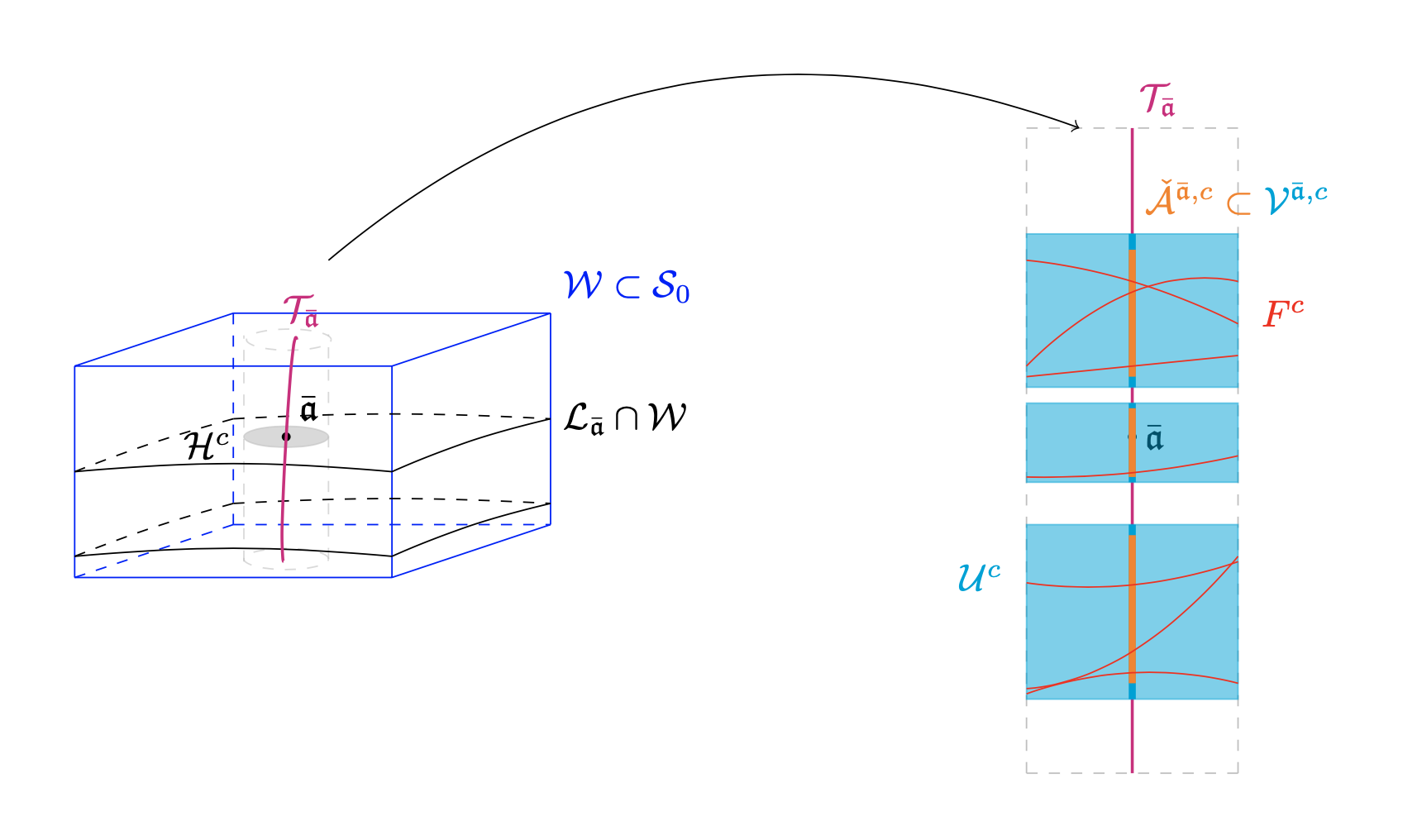
Figure 3: A picture to illustrate Lemma 8.5

Proof of Lemma 8.5.

The set $\mathcal{I}^{c}\left(\check{\mathcal{A}}^{\bar{{\mathfrak{a}}},c}\right)\cap\overline{Y^{c}}$ is a compact set which does not intersect $\partial Y^{c}$, so there is an open set $\mathcal{O}\subset\mathcal{S}_{0}$ which contains $\partial Y^{c}$ and such that $\mathcal{I}^{c}\left(\check{\mathcal{A}}^{\bar{{\mathfrak{a}}},c}\right)\cap Y^{c}\subset Y^{c}\setminus\overline{\mathcal{O}}$. As a consequence, by regularity of the mapping ${\mathfrak{a}}\in\mbox{dom}(D^{c})\mapsto\mathcal{I}^{c}({\mathfrak{a}})$, there is an open set $\mathcal{U}^{c}\subset\mathcal{W}$ containing $\check{\mathcal{A}}^{\bar{{\mathfrak{a}}},c}$ such that

$$\mathcal{D}^{c}({\mathfrak{a}})<\bar{l}+2\quad\mbox{and}\quad\mathcal{I}^{c}({\mathfrak{a}})\cap\overline{Y^{c}}\subset Y^{c}\setminus\overline{\mathcal{O}}\qquad\forall{\mathfrak{a}}\in\mathcal{U}^{c}.$$

In fact, for every ${\mathfrak{a}}\in\mathcal{U}^{c}$, the restriction of $D^{c}$ to the local leaf $\mathcal{L}_{{\mathfrak{a}}}\cap\mathcal{U}^{c}$, let us denote it by $D^{c}_{{\mathfrak{a}}}$, coincides with the distance function to the set $\widetilde{Y}^{c,{\mathfrak{a}}}:=\mathcal{L}_{{\mathfrak{a}}}\cap(Y^{c}\setminus\overline{\mathcal{O}})$ which, by the transversality property given by Lemma 8.3 (iv) and compactness of $Y^{c}\setminus\mathcal{O}\subset Y^{c}$, is the union of finitely many points. So, as a distance function from a smooth submanifold (of dimension zero) on a complete Riemannian manifold, for every ${\mathfrak{a}}\in\mathcal{U}^{c}$ the function $D^{c}_{{\mathfrak{a}}}$ satisfies the following properties:

• The function $D^{c}_{{\mathfrak{a}}}$ is locally lipschitz on $\hat{\mathcal{L}}_{{\mathfrak{a}}}:=\mathcal{L}_{{\mathfrak{a}}}\cap\mathcal{U}^{c}$ and its singular set $\Sigma(D^{c}_{{\mathfrak{a}}})$, defined as the set of points in $\hat{\mathcal{L}}_{{\mathfrak{a}}}$ where $D^{c}_{{\mathfrak{a}}}$ is not differentiable, has measure zero in $\hat{\mathcal{L}}_{{\mathfrak{a}}}$.

• Denoting by $\nabla D^{c}_{{\mathfrak{a}}}$ the gradient of $D^{c}_{{\mathfrak{a}}}$ with respect to $g^{c,{\mathfrak{a}}}$, define the limiting-gradient of $D^{c}_{{\mathfrak{a}}}$ at some point ${\mathfrak{a}}^{\prime}\in\hat{\mathcal{L}}_{{\mathfrak{a}}}$, denoted by $\nabla^{L}D^{c}_{{\mathfrak{a}}}({\mathfrak{a}}^{\prime})\subset T_{{\mathfrak{a}}^{\prime}}\mathcal{L}_{{\mathfrak{a}}}$, as the set of all limits in $T_{{\mathfrak{a}}^{\prime}}\mathcal{L}_{{\mathfrak{a}}}$ of sequences of the form $\{\nabla D^{c}_{{\mathfrak{a}}}({\mathfrak{a}}_{k})\}_{k\in\mathbb{N}}\in T_{{\mathfrak{a}}_{k}}\mathcal{L}_{{\mathfrak{a}}}$ where $\{a_{k}\}_{k\in\mathbb{N}}$ is a sequence of points in $\hat{\mathcal{L}}_{{\mathfrak{a}}}\setminus\Sigma(D^{c}_{{\mathfrak{a}}})$ converging to ${\mathfrak{a}}^{\prime}$ (note that by (P1) such sequences do exist). Then a point ${\mathfrak{a}}^{\prime}\in\hat{\mathcal{L}}_{{\mathfrak{a}}}$ belongs to $\Sigma(D^{c}_{{\mathfrak{a}}})$ if and only if $\nabla^{L}D^{c}_{{\mathfrak{a}}}({\mathfrak{a}}^{\prime})$ is not a singleton. Moreover, for every ${\mathfrak{a}}^{\prime}\in\hat{\mathcal{L}}_{{\mathfrak{a}}}$, there is a one-to-one correspondence between $\nabla^{L}D^{c}_{{\mathfrak{a}}}({\mathfrak{a}}^{\prime})$ and $\Gamma^{c}({\mathfrak{a}}^{\prime})$ (the set of all minimizing geodesics for $D^{c}({\mathfrak{a}}^{\prime})$), namely a vector $\zeta^{\prime}\in T_{{\mathfrak{a}}^{\prime}}\hat{\mathcal{L}}_{{\mathfrak{a}}^{\prime}}$ belongs to $\nabla^{L}D^{c}_{{\mathfrak{a}}}({\mathfrak{a}}^{\prime})$ if and only if the $\mathcal{L}_{{\mathfrak{a}}}$-geodesic $\psi^{{\mathfrak{a}}^{\prime},\zeta^{\prime}}:[0,1]\rightarrow\mathcal{L}_{{\mathfrak{a}}}$ (uniquely) defined by the initial conditions

  $$\psi^{{\mathfrak{a}}^{\prime},\zeta^{\prime}}(0)={\mathfrak{a}}^{\prime}\quad\mbox{and}\quad\dot{\psi}^{{\mathfrak{a}}^{\prime},\zeta^{\prime}}(0)=-\zeta^{\prime}$$

  is a minimizing geodesic for $D^{c}({\mathfrak{a}}^{\prime})$. Moreover, every such geodesic satisfies

  $$\psi^{{\mathfrak{a}}^{\prime},\zeta^{\prime}}(1)\in Z^{c,{\mathfrak{a}}}\quad\mbox{and}\quad\psi^{{\mathfrak{a}}^{\prime},\zeta^{\prime}}(t)=\beta^{{\mathfrak{a}}^{\prime},\zeta^{\prime}}(1-t)\quad\forall t\in[0,1]$$

  where $\beta^{{\mathfrak{a}}^{\prime},\zeta^{\prime}}$ is the $\mathcal{L}_{{\mathfrak{a}}}$-geodesic given by

  $$\beta(t):=\exp_{P({\mathfrak{a}}^{\prime},\zeta^{\prime})}^{c}\left(V({\mathfrak{a}}^{\prime},\zeta^{\prime})\right)\quad\forall t\in[0,1]$$

  with

  $$P({\mathfrak{a}}^{\prime},\zeta^{\prime}):=\psi^{{\mathfrak{a}}^{\prime},\zeta^{\prime}}(1)\in Z^{c,{\mathfrak{a}}}\quad\mbox{and}\quad V({\mathfrak{a}}^{\prime},\zeta^{\prime}):=-\dot{\psi}^{{\mathfrak{a}}^{\prime},\zeta^{\prime}}(1)\in T_{P({\mathfrak{a}}^{\prime},\zeta^{\prime})}\mathcal{L}_{{\mathfrak{a}}}.$$

• Let $\mbox{Conj}^{c,{\mathfrak{a}}}(\hat{\mathcal{L}_{{\mathfrak{a}}}})\subset\hat{\mathcal{L}_{{\mathfrak{a}}}}$ be the set of points ${\mathfrak{a}}^{\prime}\in\hat{\mathcal{L}_{{\mathfrak{a}}}}$ for which there is $\zeta^{\prime}\in\nabla^{L}D^{c}_{{\mathfrak{a}}}({\mathfrak{a}}^{\prime})$, called conjugate limiting-gradient of $D^{c}_{{\mathfrak{a}}}$ at ${\mathfrak{a}}^{\prime}$, such that the tangent vector $V({\mathfrak{a}}^{\prime},\zeta^{\prime})$ is a critical point of the exponential map $\exp_{P({\mathfrak{a}}^{\prime},\zeta^{\prime})}^{c}$. Then we have

  $$\mbox{Cut}^{c,{\mathfrak{a}}}\left(\hat{\mathcal{L}_{{\mathfrak{a}}}}\right):=\overline{\Sigma(D^{c}_{{\mathfrak{a}}})}=\Sigma(D^{c}_{{\mathfrak{a}}})\cup\mbox{Conj}^{c,{\mathfrak{a}}}\left(\hat{\mathcal{L}_{{\mathfrak{a}}}}\right).$$

• The set $\mbox{Cut}^{c,{\mathfrak{a}}}(\hat{\mathcal{L}_{{\mathfrak{a}}}})$, called cut locus in $\hat{\mathcal{L}_{{\mathfrak{a}}}}$, has Lebesgue measure zero in $\hat{\mathcal{L}}_{{\mathfrak{a}}}$ and the function $D^{c}_{{\mathfrak{a}}}$ is smooth on $\hat{\mathcal{L}}_{{\mathfrak{a}}}\setminus\mbox{Cut}^{c,{\mathfrak{a}}}(\hat{\mathcal{L}_{{\mathfrak{a}}}})$. In particular, for every ${\mathfrak{a}}^{\prime}\in\hat{\mathcal{L}}_{{\mathfrak{a}}}\setminus\mbox{Cut}^{c,{\mathfrak{a}}}(\hat{\mathcal{L}_{{\mathfrak{a}}}})$, the set $\nabla^{L}D^{c}_{{\mathfrak{a}}}({\mathfrak{a}}^{\prime})$ is a singleton $\{\zeta({\mathfrak{a}}^{\prime})\}$ and moreover the exponential map $\exp_{P({\mathfrak{a}}^{\prime},\zeta^{\prime})}^{c}:T_{P({\mathfrak{a}}^{\prime},\zeta^{\prime})}\mathcal{L}_{{\mathfrak{a}}}\rightarrow\mathcal{L}_{{\mathfrak{a}}}$ is a submersion at $V({\mathfrak{a}}^{\prime},\zeta^{\prime})$.

The property (P1) follows from Rademacher’s Theorem, (P2) may be found in [52, Lemma 11] (where the result is stated with Hamiltonian viewpoint) and (P3)-(P4) may be found in [16, 39, 56].

To conclude the proof of the lemma, we define the set $F^{c}\subset\mathcal{U}^{c}$ by

$$F^{c}:=\bigcup_{{\mathfrak{a}}\in\mathcal{U}^{c}}\mbox{Cut}^{c,{\mathfrak{a}}}(\hat{\mathcal{L}_{{\mathfrak{a}}}}).$$

Let us prove (i), that is, $F^{c}$ is closed in the topological subspace $\mathcal{U}^{c}$. Let $\{{\mathfrak{a}}_{k}\}_{k\in\mathbb{N}}$ be a sequence of points of $F^{c}$ converging to some ${\mathfrak{a}}\in\mathcal{U}^{c}$. Let us distinguish two cases:

Case 1: There is a constant $\delta>0$ such that the diameters (with respect to $\tilde{g}^{c}$) of the sets $\nabla^{L}D^{c}_{{\mathfrak{a}}_{k}}({\mathfrak{a}}_{k})$ are all larger than $\delta$ (so that for all $k\in\mathbb{N}$, ${\mathfrak{a}}_{k}$ belongs to $\Sigma(D^{c}_{{\mathfrak{a}}_{k}})$).
Then ${\mathfrak{a}}$ admits two minimizing geodesics $\psi_{1},\psi_{2}$ for $D^{c}({\mathfrak{a}})$ such that

$$\left|\dot{\psi}_{1}(0)-\dot{\psi}_{1}(0)\right|^{\tilde{g}^{c}}\geq\delta>0$$

so $\nabla^{L}D^{c}_{{\mathfrak{a}}_{k}}({\mathfrak{a}})$ is not a singleton (by (P2)) and ${\mathfrak{a}}$ belongs to $\Sigma(D^{c}_{{\mathfrak{a}}})\subset F^{c}$.

Case 2: There is not a constant $\delta>0$ such that the diameters (with respect to $\tilde{g}^{c}$) of the sets $\nabla^{L}D^{c}_{{\mathfrak{a}}_{k}}({\mathfrak{a}}_{k})$ are all larger than $\delta$ (so that for all $k\in\mathbb{N}$, ${\mathfrak{a}}_{k}$ belongs to $\Sigma(D^{c}_{{\mathfrak{a}}_{k}})$).
Then we have

$$\lim_{k\rightarrow\infty}\mbox{diam}^{\tilde{g}^{c}}\nabla^{L}D^{c}_{{\mathfrak{a}}_{k}}({\mathfrak{a}}_{k})=0.$$

Let us again distinguish between two cases.

Subcase 2.1: There are infinitely many $k\in\mathbb{N}$ for which ${\mathfrak{a}}_{k}$ belongs to $\mbox{Conj}^{c,{\mathfrak{a}}_{k}}(\hat{\mathcal{L}}_{{\mathfrak{a}}_{k}})$.
Then, by considering a subsequence of $\{V({\mathfrak{a}}_{k},\zeta_{k})\}_{k\in\mathbb{N}}$ with $\zeta_{k}$ a conjugate limiting-gradient of $D^{c}_{{\mathfrak{a}}_{k}}$ at ${\mathfrak{a}}_{k}$, there is a tangent vector $V({\mathfrak{a}},\zeta)$ which is a critical point of the exponential map $\exp_{P({\mathfrak{a}},\zeta)}^{c}$ as limit of the sequence of critical vectors $\{V({\mathfrak{a}}_{k},\zeta_{k})\}_{k\in\mathbb{N}}$ (with respect to $\exp_{P({\mathfrak{a}}_{k},\zeta_{k})}^{c}$). Therefore, ${\mathfrak{a}}$ belongs to $\mbox{Conj}^{c,{\mathfrak{a}}}(\hat{\mathcal{L}}_{{\mathfrak{a}}})\subset F^{c}$ by (P3).

Subcase 2.2: The set of $k\in\mathbb{N}$ for which ${\mathfrak{a}}_{k}$ belongs to $\mbox{Conj}^{c,{\mathfrak{a}}_{k}}(\hat{\mathcal{L}}_{{\mathfrak{a}}_{k}})$ is finite.
If ${\mathfrak{a}}\notin\mbox{Cut}^{c,{\mathfrak{a}}}(\hat{\mathcal{L}_{{\mathfrak{a}}}})$, then by (P2) the limiting-gradient $\nabla^{L}D^{c}_{{\mathfrak{a}}}({\mathfrak{a}})$ is equal to a singleton $\{\zeta\}$ and there is only one minimizing geodesics for $D^{c}({\mathfrak{a}})$ given by $\psi^{{\mathfrak{a}},\zeta}$. Thus, by (P3), up to considering a subsequence, we may assume without loss of generality that for all $k\in\mathbb{N}$ there are $\zeta_{k}^{1},\zeta_{k}^{2}$ in $\nabla^{L}D^{c}_{{\mathfrak{a}}_{k}}({\mathfrak{a}}_{k})$ such that

$$\zeta_{k}^{1}\neq\zeta_{k}^{2}\quad\mbox{and}\quad\lim_{k\rightarrow\infty}\left|\zeta_{k}^{1}-\zeta_{k}^{2}\right|^{\tilde{g}^{c}}=0$$

and for $i=1,2$

$$\lim_{k\rightarrow\infty}\zeta_{i}^{k}=\zeta,\quad\lim_{k\rightarrow\infty}P({\mathfrak{a}}_{k},\zeta_{i}^{k})=P({\mathfrak{a}},\zeta),\quad\lim_{k\rightarrow\infty}V({\mathfrak{a}}_{k},\zeta_{i}^{k})=V({\mathfrak{a}},\zeta).$$

Since ${\mathfrak{a}}\notin\mbox{Cut}^{c,{\mathfrak{a}}}(\hat{\mathcal{L}_{{\mathfrak{a}}}})$, (P4) shows that the exponential map $\exp_{P({\mathfrak{a}},\zeta)}^{c}:T_{P({\mathfrak{a}},\zeta)}\mathcal{L}_{{\mathfrak{a}}}\rightarrow\mathcal{L}_{{\mathfrak{a}}}$ is a submersion at $V({\mathfrak{a}},\zeta)$. So the mappings $\exp_{P({\mathfrak{a}}_{k},\zeta_{k})}^{c}:T_{P({\mathfrak{a}}_{k},\zeta_{k})}\mathcal{L}_{{\mathfrak{a}}_{k}}\rightarrow\mathcal{L}_{{\mathfrak{a}}_{k}}$ are submersions at $V({\mathfrak{a}}_{k},\zeta_{k})$ for $k$ large enough but this is impossible because

$$\exp_{P({\mathfrak{a}}_{k},\zeta_{k})}^{c}\left(V({\mathfrak{a}}_{k},\zeta_{1}^{k})\right)=\exp_{P({\mathfrak{a}}_{k},\zeta_{k})}^{c}\left(V({\mathfrak{a}}_{k},\zeta_{2}^{k})\right)\qquad\forall k\in\mathbb{N}.$$

So we have ${\mathfrak{a}}\in\mbox{Cut}^{c,{\mathfrak{a}}}(\hat{\mathcal{L}_{{\mathfrak{a}}}})$.

To prove (ii), we just notice that $\mathcal{U}^{c}$ is foliated by the leaves $\hat{\mathcal{L}}_{{\mathfrak{a}}}$ whose intersection with $F^{c}$ has measure zero by (P4). So, we get the result by a Fubini argument.

The point (iii) is a consequence of the fact that $\nabla^{L}D^{c}_{{\mathfrak{a}}}({\mathfrak{a}})$ is a singleton $\{\zeta^{{\mathfrak{a}}}\}$ for all ${\mathfrak{a}}$ in the open set $\mathcal{U}^{c}\setminus F^{c}$ together with the fact that $\exp_{P({\mathfrak{a}},\zeta^{{\mathfrak{a}}})}^{c}:T_{P({\mathfrak{a}},\zeta^{{\mathfrak{a}}})}\mathcal{L}_{{\mathfrak{a}}}\rightarrow\mathcal{L}_{{\mathfrak{a}}}$ is a submersion at $V({\mathfrak{a}},\zeta^{{\mathfrak{a}}})$ which implies that the mapping $\mbox{Exp}^{c}$ is a submersion at $(P({\mathfrak{a}},\zeta^{{\mathfrak{a}}}),V({\mathfrak{a}},\zeta^{{\mathfrak{a}}}))$. As a matter of fact, if ${\mathfrak{a}}\in\mathcal{U}^{c}\setminus F^{c}$ is fixed, then there is an open neighborhood $N$ of $(P({\mathfrak{a}},\zeta^{{\mathfrak{a}}}),V({\mathfrak{a}},\zeta^{{\mathfrak{a}}}))$ in $\vec{\mathcal{K}}_{Y^{c}}\subset T\Delta^{\perp}$ such that the image $\mbox{Exp}^{c}(N)$ is an open neighborhood of ${\mathfrak{a}}$ and we have necessarily for every $(P,V)\in N$,

$$\nabla^{L}D^{c}_{A}(A)=\left\{\zeta^{A}\right\}=\left\{-\dot{\psi}^{(P,V)}(0)\right\}\quad\mbox{with}\quad A=A(P,V):=\mbox{Exp}^{c}(P,V),$$

where $\psi^{(P,V)}:[0,1]\rightarrow\mathcal{L}_{(P,V)}$ is the $\mathcal{L}_{(P,V)}$-geodesic given by

$$\psi^{(P,V)}(t):=\mbox{Exp}^{c}(P,(1-t)V)=\exp_{(P,V)}^{c}((1-t)V)\qquad\forall t\in[0,1],$$

because $\psi^{(P,V)}$ is the only $\mathcal{L}_{(P,V)}$-geodesic closed to $\psi^{{\mathfrak{a}},\zeta^{{\mathfrak{a}}}}$ joining $A$ to $Z^{c,A}$. Since the mapping

$$A\,\longmapsto\,-\frac{d}{dt}\left\{\psi^{\bigl{(}\mbox{Exp}^{c}\bigr{)}^{-1}(A)}\right\}(0)$$

is smooth we infer that $D^{c}$ is smooth on $\mathcal{U}^{c}\setminus F^{c}$ and that $\Gamma^{c}({\mathfrak{a}})$ is a singleton for ${\mathfrak{a}}\in\mathcal{U}^{c}\setminus F^{c}$ because $\nabla^{L}D^{c}_{{\mathfrak{a}}}({\mathfrak{a}})$ is always a singleton (see (P1)).

To prove (iv), we first notice that, up to shrink $\mathcal{U}^{c}$, we may assume that for every ${\mathfrak{a}}\in\mathcal{H}^{c}$, the mapping $H^{c}$ is injective. As a matter of fact, suppose for contradiction that there are ${\mathfrak{a}}\in\mathcal{H}^{c}$ and

$$({\mathfrak{a}}_{1},t_{1}),({\mathfrak{a}}_{2},t_{2})\in\left(\left(\mathcal{U}^{c}\setminus F^{c}\right)\cap\mathcal{T}_{{\mathfrak{a}}}\right)\times[0,1]$$

such that

$$H^{c}({\mathfrak{a}}_{1},t_{1})=\psi^{c,{\mathfrak{a}}_{1}}(t_{1})=\psi^{c,{\mathfrak{a}}2}(t_{2})=H^{c}({\mathfrak{a}}_{2},t_{2}).$$

Since $\psi^{c,{\mathfrak{a}}_{1}}$ and $\psi^{c,{\mathfrak{a}}_{2}}$ are minimizing the length (among curves with are horizontal with respect to the foliation) we have either ${\mathfrak{a}}_{1}={\mathfrak{a}}_{2}$ and $\psi^{c,{\mathfrak{a}}_{1}}=\psi^{c,{\mathfrak{a}}2}$ (because $\Gamma^{c}({\mathfrak{a}}_{1})=\Gamma^{c}({\mathfrak{a}}_{2})$ is a singleton), or we have ${\mathfrak{a}}_{1}\neq{\mathfrak{a}}_{2}$ and $t_{1}=t_{2}=1$. In the latter case, we infer that ${\mathfrak{a}}_{1}$ and ${\mathfrak{a}}_{2}$ belong to the same leaf $\mathcal{L}_{{\mathfrak{a}}_{1}}=\mathcal{L}_{{\mathfrak{a}}_{2}}$ and can be connect by a curve horizontal (with respect to $\mathcal{L}_{{\mathfrak{a}}_{1}}$) of length $<2\bar{\ell}+4$. By Lemma 8.2 (iii), this cannot occur if the open neighborhood $\mathcal{U}^{c}\subset\mathcal{W}$ of $\check{\mathcal{A}}^{\bar{{\mathfrak{a}}},c}$ is sufficiently small. The smoothness of $H^{c}$ follows from (iii) and the property of diffeomorphism is a consequence of the fact that all minimizing curves from $\mathcal{U}^{c}$ to $\bar{Y}^{c}\setminus\mathcal{O}$ have no conjugate times.

We conclude easily the construction of $\mathcal{V}^{c,\bar{{\mathfrak{a}}}}\subset\mathcal{T}_{\bar{{\mathfrak{a}}}}$ and $\mathcal{H}^{c}$ of $\bar{{\mathfrak{a}}}\subset\mathcal{L}_{\bar{{\mathfrak{a}}}}$. ∎

The following lemma will allow us to conclude the proof of Theorem 1.5, it follows easily from Lemma 8.5.

Lemma 8.6.

For every $0<c<\epsilon$, there are ${\mathfrak{a}}^{c}\in\mathcal{L}_{\bar{{\mathfrak{a}}}}\cap\mathcal{W}$, a finite set $J^{c}$, two collections of sets $\{\mathcal{O}_{j}^{c,0}\}_{j\in J^{c}}$, $\{\mathcal{O}_{j}^{c,1}\}_{j\in J^{c}}$ and a collection of functions $\{\Phi_{j}^{c}:\mathcal{O}_{j}^{c,0}\times[0,1]\rightarrow\mathcal{S}_{0}\}_{j\in J^{c}}$ satisfying the following properties:

• The sets $\mathcal{O}_{j}^{c,0}$ (with $j\in J^{c}$) are pairwise disjoint.

• The sets $\mathcal{O}_{j}^{c,1}$ (with $j\in J^{c}$) are pairwise disjoint.

• For every $j\in J^{c}$, $\mathcal{O}_{j}^{c,0}$ is a compact, connected and oriented, smooth submanifold with boundary of $\mathcal{T}_{{\mathfrak{a}}^{c}}$ of dimension $r$.

• For every $j\in J^{c}$, $\mathcal{O}_{j}^{c,1}$ is a compact, connected and oriented, smooth submanifold with boundary of $Y^{c}\subset X^{c}$ of dimension $r$.

• For every $j\in J^{c}$, $\Phi_{j}^{c}:\mathcal{O}_{j}^{c,0}\times[0,1]\rightarrow\mathcal{S}_{0}$ is smooth and for every $t\in[0,1]$, the restriction of $\Phi_{j}^{c}$ to $\mathcal{O}_{j}^{c,0}\times\{t\}$ is a diffeomorphism from $\mathcal{O}_{j}^{c,0}\times\{t\}$ to its image

  $$\mathcal{O}_{j}^{c,t}:=\Phi_{j}^{c}\left(\mathcal{O}_{j}^{c,0}\times\{t\}\right).$$

  In particular, $\Phi_{j}^{c}({\mathfrak{a}},0)={\mathfrak{a}}$ for every ${\mathfrak{a}}\in\mathcal{O}_{j}^{c,0}$ and $\mathcal{O}_{j}^{c,1}$ is the diffeomorphic image of $\mathcal{O}_{j}^{c,0}\times\{1\}$ by $\Phi_{j}^{c}$.

• For every $j\in J^{c}$ and any $t,t^{\prime}\in[0,1]$ with $t\neq t^{\prime}$, $\mathcal{O}_{j}^{c,t}\cap\mathcal{O}_{j}^{c,t^{\prime}}=\emptyset$.

• For every $j\in J^{c}$ and every ${\mathfrak{a}}\in\mathcal{O}_{i}^{c,0}$, the smooth curve $t\in[0,1]\rightarrow\Phi_{i}^{c}({\mathfrak{a}},t)$ is a $\mathcal{L}_{{\mathfrak{a}}}$-geodesic with non zero speed.

• The set $\mathcal{O}^{c,0}:=\cup_{j\in J^{c}}\mathcal{O}_{j}^{c,0}$ has measure $\geq\nu/16$ with respect to the volume form $\eta_{|\mathcal{T}_{\bar{{\mathfrak{a}}}}}$.

Proof of Lemma 8.6.

Fix $0<c<\epsilon$ and consider the sets $\mathcal{V}^{c,\bar{{\mathfrak{a}}}}\subset\mathcal{T}_{\bar{{\mathfrak{a}}}}$, $\mathcal{H}^{c}\subset\mathcal{L}_{\bar{{\mathfrak{a}}}}$, $F^{c}\subset\mathcal{S}_{0}$ and $\mathcal{U}^{c}\subset\mathcal{W}$ given by Lemma 8.5. The set $\mathcal{U}^{c}$ is foliated by the leaves $\mathcal{V}^{c,\bar{{\mathfrak{a}}}}_{{\mathfrak{a}}}$ with ${\mathfrak{a}}\in\mathcal{H}^{c}$ and by Lemma 8.5 (i), the set $F^{c}\cap\mathcal{U}^{c}$ has Lebesgue measure zero. Hence Fubini’s Theorem implies that there is ${\mathfrak{a}}^{c}\in\mathcal{H}^{c}$ such that the set $F^{c}\cap\mathcal{V}^{c,\bar{{\mathfrak{a}}}}_{{\mathfrak{a}}^{c}}\subset\mathcal{T}_{{\mathfrak{a}}^{c}}$ has measure zero. Without loss of generality, up to shrinking $\mathcal{V}^{c,\bar{{\mathfrak{a}}}}_{{\mathfrak{a}}^{c}}$ in $\mathcal{T}_{{\mathfrak{a}}^{c}}$ we may assume that

$$\overline{\mathcal{V}^{c,\bar{{\mathfrak{a}}}}_{{\mathfrak{a}}^{c}}}\subset\mathcal{T}_{{\mathfrak{a}}^{c}}$$

and moreover, by Lemma 8.4 (iii), we may assume by taking ${\mathfrak{a}}^{c}$ sufficiently close to $\bar{{\mathfrak{a}}}$ that the compact set $\check{\mathcal{A}}^{\bar{{\mathfrak{a}}},c}_{{\mathfrak{a}}^{c}}\subset\mathcal{T}_{{\mathfrak{a}}^{c}}$ has measure $\geq\nu/8$ with respect to the volume form $\eta_{|\mathcal{T}_{{\mathfrak{a}}^{c}}}$. Consider a smooth function $G_{c}:\mathcal{T}_{{\mathfrak{a}}^{c}}\rightarrow[0,\infty)$ such that

$$G^{-1}_{c}\left(\{0\}\right)=\left(F^{c}\cap\mathcal{V}^{c,\bar{{\mathfrak{a}}}}_{{\mathfrak{a}}^{c}}\right)\cup\partial\mathcal{V}^{c,\bar{{\mathfrak{a}}}}_{{\mathfrak{a}}^{c}}$$

and set for every $\epsilon>0$,

$$\Omega^{c}_{\epsilon}:=G^{-1}_{c}\bigl{(}[\epsilon,\infty)\bigr{)}\cap\mathcal{V}^{c,\bar{{\mathfrak{a}}}}_{{\mathfrak{a}}^{c}}.$$

By Sard’s Theorem, $G_{c}$ admits a decreasing sequence $\{\epsilon_{k}\}_{k\in\mathbb{N}}$ of regular values converging to $0$. Thus we have

$$\mathcal{V}^{c,\bar{{\mathfrak{a}}}}_{{\mathfrak{a}}^{c}}=\bigcup_{k\in\mathbb{N}}\Omega^{c}_{\epsilon_{k}}\quad\mbox{with}\quad\Omega^{c}_{\epsilon_{k}}\subset\Omega^{c}_{\epsilon_{k+1}}\quad\forall k\in\mathbb{N}$$

and for every $k\in\mathbb{N}$ the set $\Omega^{c}_{\epsilon_{k}}$ is a compact, oriented, smooth submanifold with boundary of $\mathcal{T}_{{\mathfrak{a}}^{c}}$ of dimension $r$. As a consequence, since the measure of $\mathcal{V}^{c,\bar{{\mathfrak{a}}}}_{{\mathfrak{a}}^{c}}$, which contains $\check{\mathcal{A}}^{\bar{{\mathfrak{a}}},c}_{{\mathfrak{a}}^{c}}$, with respect to the volume form $\eta_{|\mathcal{T}_{{\mathfrak{a}}^{c}}}$ is $\geq\nu/8$, there is $\bar{k}\in\mathbb{N}$ large enough such that the measure (with respect to the volume form $\eta_{|\mathcal{T}_{{\mathfrak{a}}^{c}}}$) of the set

$$\mathcal{O}^{c,0}:=\Omega^{c}_{\epsilon_{\bar{k}}}$$

is $\geq\nu/16$. By construction, $\mathcal{O}^{c,0}$ is the union of finitely many components $\mathcal{O}^{c,0}_{j}$ satisfying properties (i), (iii), (viii) of the statement, where $j$ varies in a finite set $J^{c}$. Then, for every $j\in J^{c}$, we define $\Phi_{j}^{c}:\mathcal{O}_{j}^{c,0}\times[0,1]\rightarrow\mathcal{S}_{0}$ by

$$\Phi_{j}^{c}:=H^{c}_{|\mathcal{O}_{j}^{c,0}\times[0,1]}$$

and we set

$$\mathcal{O}_{j}^{c,1}:=\Phi_{j}^{c}\left(\mathcal{O}_{j}^{c,0}\times\{1\}\right).$$

The properties (ii), (iv), (v), (vi) and (vii) are satisfied by the construction together with Lemma 8.5 (iv). ∎

We are now ready to complete the proof of Theorem 1.5. Let us temporarily fix $0<c<\epsilon$. By Lemma 8.6, there are a finite set $J^{c}$, two collections of sets $\{\mathcal{O}_{j}^{c,0}\}_{j\in J^{c}}$, $\{\mathcal{O}_{j}^{c,1}\}_{j\in^{c}}$ and a collection of functions $\{\Phi_{j}^{c}:\mathcal{O}_{j}^{c,0}\times[0,1]\rightarrow\mathcal{S}_{0}\}_{j\in J^{c}}$ such that the properties (i)-(viii) are satisfied. Set for every $j\in J^{c}$ (see Figure 4)

$$\mathcal{M}^{c}_{j}:=\Bigl{\{}\Phi_{j}^{c}({\mathfrak{a}},t)\,|\,({\mathfrak{a}},t)\in\mathcal{O}_{j}^{c}\times[0,1]\Bigr{\}}.$$

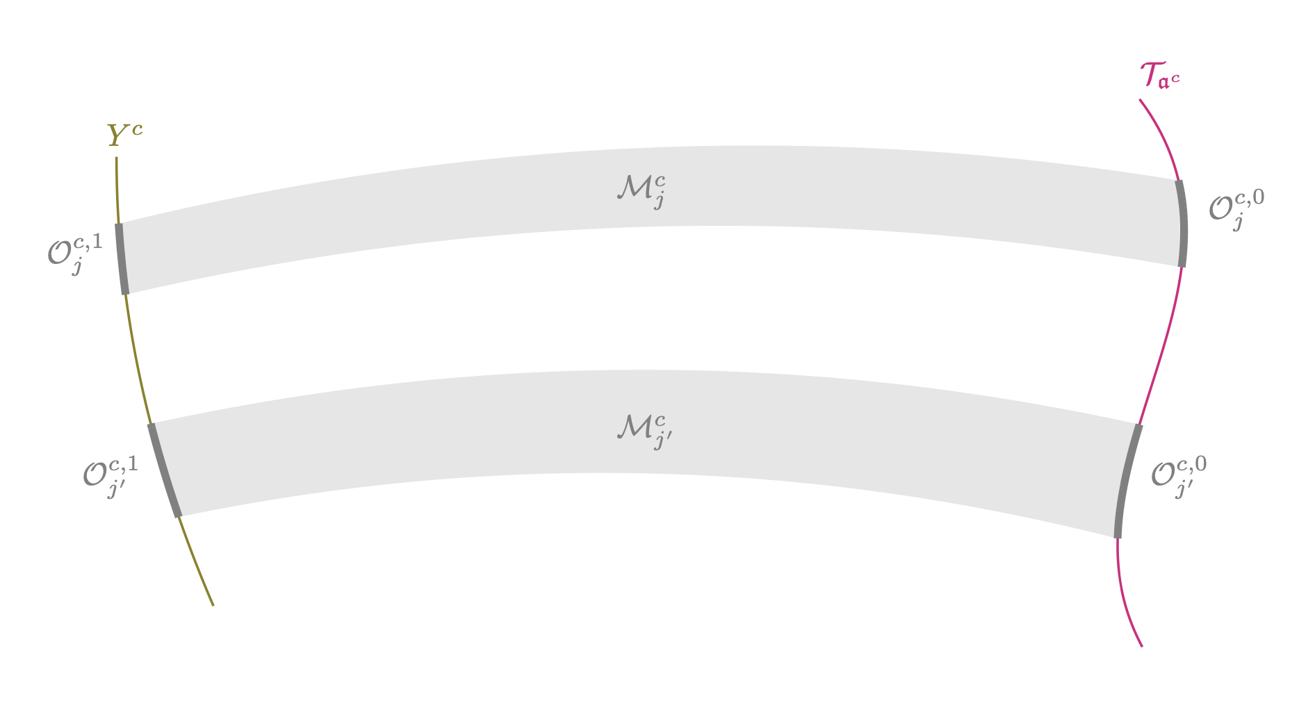
Figure 4: The sets $\mathcal{O}_{j}^{c,0},\mathcal{O}_{j}^{c,1}$ and $\mathcal{M}_{j}^{c}$

By properties (iii)-(vii), it is a topological manifold (with boundary) of dimension $r+1$ whose boundary can be written as

$$\partial\mathcal{M}_{j}^{c}=\mathcal{O}_{j}^{c,0}\cup\mathcal{O}_{j}^{c,1}\cup\mathcal{C}^{c}_{j}$$

where both $\mathcal{O}_{j}^{c,0}$ and $\mathcal{O}_{j}^{c,1}$ are compact, connected, oriented, smooth submanifolds with boundary (Lemma 8.6 (iii)-(iv)) and where the cylindrical part $\mathcal{C}^{c}_{j}$ given by

$$\mathcal{C}^{c}_{j}:=\Bigl{\{}\Phi_{j}^{c}({\mathfrak{a}},t)\,|\,({\mathfrak{a}},t)\in\partial\mathcal{O}_{j}^{c,0}\times(0,1)\Bigr{\}}$$

is a smooth open oriented submanifold of dimension $r=2l$ satisfying

$$\eta_{|\mathcal{C}^{c}_{j}}=0,$$

because any point of $\mathcal{C}^{c}_{j}$ has the form $\Phi_{j}^{c}({\mathfrak{a}},t)$ with ${\mathfrak{a}}\in\partial\mathcal{O}_{j}^{c,0}$ and (by Lemma 8.6 (vii))

$$0\neq\frac{\partial\Phi_{j}^{c}}{\partial t}({\mathfrak{a}},t)\in\left(T_{\Phi_{j}^{c}({\mathfrak{a}},t)}\mathcal{C}_{j}^{c}\right)\cap\left(T_{\Phi_{j}^{c}({\mathfrak{a}},t)}\mathcal{L}_{{\mathfrak{a}}}\right)$$

$$\mbox{with}\quad T_{\Phi_{j}^{c}({\mathfrak{a}},t)}\mathcal{L}_{{\mathfrak{a}}}=\vec{\mathcal{K}}\left(\Phi_{j}^{c}({\mathfrak{a}},t)\right)=\mbox{ker}\left(\omega^{\perp}_{\Phi_{j}^{c}({\mathfrak{a}},t)}\right).$$

As a consequence, by applying Stokes’ Theorem we have for every $j\in J^{c}$,

$$\int_{\mathcal{O}_{j}^{c,0}}\eta=\int_{\mathcal{O}_{j}^{c,1}}\eta,$$

which imply (because, by Lemma 8.6 (i)-(ii), the sets $\mathcal{O}_{j}^{c,0}$ (resp. $\mathcal{O}_{j}^{c,1}$) are pairwise disjoint)

$$\int_{\mathcal{O}^{c,0}}\eta=\int_{\cup_{j\in J^{c}}\mathcal{O}_{j}^{c,0}}\eta=\sum_{j\in J^{c}}\int_{\mathcal{O}_{j}^{c,0}}\eta=\sum_{j\in J^{c}}\int_{\mathcal{O}_{j}^{c,1}}\eta=\int_{\cup_{j\in J^{c}}\mathcal{O}_{j}^{c,1}}\eta=\int_{\mathcal{O}^{c,1}}\eta.$$ (8.8)

But, on the one hand, by Lemma 8.6 (viii), we have

$$\int_{\mathcal{O}^{c,0}}\eta\geq\frac{\nu}{16},$$

and, on the other hand Lemma 8.3 (ii) together with equation (8.5) yield ($\tilde{g}_{|X^{c}}$ denotes the metric induced by $\tilde{g}$ on $X^{c}$)

$$\left|\int_{\mathcal{O}^{c,1}}\eta\right|\leq\int_{\mathcal{O}^{c,1}}|\eta|\leq\int_{\mathcal{O}^{c,1}}\delta(c)\,d\mbox{vol}^{\tilde{g}_{|X^{c}}}\leq\int_{X^{c}}\delta(c)\,d\mbox{vol}^{\tilde{g}_{|X^{c}}}\leq\delta(c)\,C,$$

which tends to zero as $c$ tends to zero. Thus (8.8) cannot be satisfied for all $c>0$, this is a contradiction.

Appendix A The Sussmann regularity Theorem

The following result concerned with the regularity of singular minimizing geodesics in sub-Riemannian geometry, due to Sussmann [59], can be seen as an application of Theorem 1.1. For further details of sub-Riemannian geometry, we refer the reader to Bellaïche’s monograph [6], or to the books by Montgomery [45], by Agrachev, Barilari and Boscain [2], or by the third author [53].

Theorem A.1 (Sussmann’s regularity Theorem [59]).

Assume that $M$ and $\Delta$ are analytic and that $g$ is smooth (resp. analytic). Then any minimizing geodesic is smooth (resp. analytic) on an open dense subset of its interval of definition.

Proof of Theorem A.1.

As in [59], we prove the result by induction on the rank of the distribution $\Delta$. So, we are going to show the following property, called $(P_{m})$, for every integer $m\geq 1$:

$(P_{m}):$ If $\Delta$ is an analytic totally nonholonomic distribution of rank $m\geq 1$ equipped with a smooth (resp. analytic) metric $g$ on a real-analytic manifold $N$ of dimension $n\geq m$ and $\gamma:[a,b]\rightarrow N$ is a minimizing geodesic, then $\gamma$ is smooth (resp. analytic) on an open dense subset of $[a,b]$.

Firstly, the property $(P_{1})$ holds true because if $m=1$ then $n=1$ and any geodesic is smooth (resp. analytic) on its interval of definition. Let us now assume that for some integer $m\geq 1$, $(P_{k})$ holds true for any integer $k\in[1,m]$, and show that $(P_{m+1})$ is satisfied. Let $\Delta$ be an analytic totally nonholonomic distribution of rank $m+1$ equipped with a smooth (resp. analytic) metric $g$ on a real-analytic manifold $M$ of dimension $n\geq m+1$ and let $\gamma:[a,b]\rightarrow M$ be a minimizing geodesic. If $\gamma$ is nonsingular, then it is the projection of a trajectory of the Hamiltonian vector field in $T^{*}M$ associated with $(\Delta,g)$, so it is smooth (resp. analytic) (see [53]). So, we assume from now that $\gamma$ is singular. By Theorem 1.1, there is a subanalytic distribution $\vec{\mathcal{K}}\subset\vec{\Delta}$ of rank $\leq m-1$ on $\Delta^{\perp}\subset T^{*}M$ associated with a subanalytic stratification $\mathcal{S}=(\mathcal{S}_{\alpha})$ of $\Delta^{\perp}$ and $\gamma$ is the projection of an absolutely continuous curve $\psi:[a,b]\rightarrow\Delta^{\perp}$ such that

$$\dot{\psi}(t)\in\vec{\mathcal{K}}(\psi(t))\subset T_{\psi(t)}(T^{*}M)\qquad\mbox{for a.e. }t\in[a,b].$$ (A.1)

Moreover, the metric $g$ on $M$ can be lifted to a metric $\tilde{g}$ over $\vec{\Delta}$ by setting for every ${\mathfrak{a}}\in\Delta^{\perp}$,

$$\tilde{g}_{{\mathfrak{a}}}(\xi_{1},\xi_{2}):=g_{\pi({\mathfrak{a}})}(d_{{\mathfrak{a}}}\pi(\xi_{1}),d_{{\mathfrak{a}}}\pi(\xi_{2}))\qquad\forall\xi_{1},\xi_{2}\in\vec{\Delta}({\mathfrak{a}}).$$

By construction, $\tilde{g}$ is smooth (resp. analytic) if $g$ is smooth (resp. analytic) and the curve $\psi$ minimizes the length with respect to $\tilde{g}$ among all horizontal paths of $\vec{\mathcal{K}}$ joining $\psi(a)$ to $\psi(b)$. Let $D\in\{1,\ldots,m-1\}$ be the maximum of $d\geq 1$ such that there are $t\in[a,b]$ and $\alpha$ with $\psi(t)\in\mathcal{S}_{\alpha}$ and $\dim(\mathcal{S}_{\alpha})=d$, then let $\mathcal{S}^{D}$ be the real-analytic manifold defined as the union of all strata $\mathcal{S}_{\alpha}$ of dimension $D$. By construction, the set

$$I_{D}:=\Bigl{\{}t\in(a,b)\,|\,\psi(t)\in\mathcal{S}^{D}\Bigr{\}}$$

is an open set. Moreover since $\vec{\mathcal{K}}$ has constant rank and is totally nonholonomic on each analytic leaf generated by $\vec{\mathcal{J}}$, we infer by the induction hypothesis that $\psi$ is smooth (resp. analytic) on an open dense subset of $I_{D}$. Now we can repeat this construction with the restriction of $\psi$ to the open set given by the interior of $(0,1)\setminus I_{D}$ and observe that the set $((0,1)\setminus I_{D})\setminus\mbox{Int}((0,1)\setminus I_{D})$ has empty interior. In conclusion, we obtain that $\psi$ is smooth (resp. analytic) on an open dense subset of $[a,b]$ and as a consequence that $\gamma=\pi(\psi)$ satisfies the same property. ∎

Appendix B Proof of results of Section 2.4

Let $v_{1},\ldots,v_{m}$ be a basis of $V$ and $X^{1},\ldots,X^{m}$ the left-invariant vector fields defined by

$$X^{i}(g)=d_{e}L_{x}(v_{i})\qquad\forall g\in\mathbb{G},\,\forall i=1,\ldots,m.$$

Then the totally nonholonomic left-invariant distribution $\Delta$ associated to $V$ satisfies

$$\Delta(g)=\mbox{Span}\Bigl{\{}X^{1}(g),\cdots,X^{m}(g)\Bigr{\}}=d_{e}L_{g}(V)\qquad\forall g\in\mathbb{G}$$

and we have (see (3.5))

$$\mbox{ker}\bigl{(}\omega^{\perp}_{{\mathfrak{a}}}\bigr{)}=\vec{\Delta}({\mathfrak{a}})\cap\,T_{{\mathfrak{a}}}\Delta^{\perp}\qquad\forall{\mathfrak{a}}\in\Delta^{\perp},$$ (B.1)

where $\vec{\Delta}$ is the distribution on $T^{*}M$ defined by

$$\vec{\Delta}({\mathfrak{a}}):=\Bigl{\{}\vec{h}^{1}({\mathfrak{a}}),\ldots,\vec{h}^{m}({\mathfrak{a}})\Bigr{\}}\qquad\forall\,{\mathfrak{a}}\in T^{*}\mathbb{G}$$

and where for every $i=1,\ldots,m$, $h^{i}$ stands for the Hamiltonian $h^{X^{i}}:T^{*}\mathbb{G}\rightarrow\mathbb{R}$ associated with $X^{i}$. Let us now see how $\Phi=(\Phi_{1},\Phi_{2}):T^{*}\mathbb{G}\rightarrow\mathbb{G}\times\mathfrak{g}^{*}$ (defined by (2.2)) pushes forward the vector fields $\vec{h}^{1},\ldots,\vec{h}^{m}$. We need the following lemma.

Lemma B.1.

For every left-invariant vector field $X$ on $\mathbb{G}$ with $v:=X(e)\in\mathfrak{g}$, we have

$$d_{{\mathfrak{a}}}\Phi_{1}\left(\vec{h}^{X}(g,p)\right)=X(g)\quad\mbox{and}\quad d_{{\mathfrak{a}}}\Phi_{2}\left(\vec{h}^{X}(g,p)\right)=-p\cdot d_{e}L_{g}([v,\cdot]),$$

for every ${\mathfrak{a}}=(g,p)\in T^{*}\mathbb{G}$.

Proof of Lemma B.1.

Let $X$ an invariant vector field be fixed and $v:=X(e)\in\mathfrak{g}$. The first part follows directly from the fact that $\Phi_{2}$ coincides with the canonical projection from $T^{*}\mathbb{G}$ to $\mathbb{G}$ and the definition of the Hamiltonian vector field $\vec{h}^{X}$, see Section 3.1. For the second part, we need to show that

$$d_{(g,p)}\Phi_{2}\left(\vec{h}^{X}(g,p)\right)(w)=-p\cdot d_{e}L_{g}([v,w])\qquad\forall w\in\mathfrak{g},\,\forall{\mathfrak{a}}=(g,p)\in T^{*}\mathbb{G}.$$

So, fix ${\mathfrak{a}}=(g,p)\in T^{*}\mathbb{G}$, $w\in\mathfrak{g}$, and moreover denote by $Y$ the left-invariant vector field verifying $Y(e)=w$ and by $\varphi_{t}({\mathfrak{a}})=(g(t),p(t))$ the trajectory of the flow of $\vec{h}^{X}$ passing through ${\mathfrak{a}}$ at time $t=0$. We have

$$d_{{\mathfrak{a}}}\Phi_{2}\left(\vec{h}^{X}({\mathfrak{a}})\right)(w) = \frac{d}{dt}\Bigl{\{}\Phi_{2}\bigl{(}\varphi_{t}({\mathfrak{a}})\bigr{)}(w)\Bigr{\}}_{|t=0}$$

$$= \frac{d}{dt}\Bigl{\{}\Phi_{2}\bigl{(}g(t),p(t)\bigr{)}(w)\Bigr{\}}_{|t=0}$$

$$= \frac{d}{dt}\Bigl{\{}\bigl{(}p(t)\cdot d_{e}L_{g(t)}\bigr{)}(w)\Bigr{\}}_{|t=0}$$

$$= \frac{d}{dt}\Bigl{\{}p(t)\cdot\left(d_{e}L_{g(t)}(w)\right)\Bigr{\}}_{|t=0}$$

$$= \frac{d}{dt}\Bigl{\{}p(t)\cdot Y\bigl{(}g(t)\bigr{)}\Bigr{\}}_{|t=0}$$

$$= \frac{d}{dt}\Bigl{\{}h^{Y}\bigl{(}g(t),p(t)\bigr{)}\Bigr{\}}_{|t=0}$$

$$= \vec{h}^{X}\cdot h^{Y}(g,p),$$

which by Proposition 3.1 gives

$$d_{{\mathfrak{a}}}\Phi_{2}\left(\vec{h}^{X}({\mathfrak{a}})\right)(w)=-h^{[X,Y]}(g,p)=-p\cdot\bigl{(}[X,Y](g)\bigr{)}=-\left(p\cdot d_{e}L_{g}\right)([v,w]),$$

which proves the result. ∎

Therefore, by Lemma B.1, for every ${\mathfrak{a}}=(g,p)\in T^{*}\mathbb{G}$, the linear space $\vec{\Delta}({\mathfrak{a}})$ is sent to

$$\vec{\mathfrak{D}}(g,\mathfrak{p}):=d_{{\mathfrak{a}}}\Phi\left(\vec{\Delta}({\mathfrak{a}})\right)=\left\{\left(\begin{array}[]{c}d_{e}L_{g}(v)\\ -\mathfrak{p}\cdot[v,\cdot]\end{array}\right)\,|\,v\in V\right\}\quad\mbox{ with}\quad\mathfrak{p}=\Phi_{2}({\mathfrak{a}}).$$

Moreover, we have $\Phi(\Delta^{\perp})=\mathbb{G}\times V^{\perp}$ and for every $(g,\mathfrak{p})\in\mathbb{G}\times V^{\perp}$,

$$\vec{\mathfrak{D}}(g,\mathfrak{p})\cap\,T_{(g,\mathfrak{p})}\left(\mathbb{G}\times V^{\perp}\right) = \left\{\left(\begin{array}[]{c}d_{e}L_{g}(v)\\ -\mathfrak{p}\cdot[v,\cdot]\end{array}\right)\,|\,v\in V\mbox{ s.t. }\mathfrak{p}\cdot[v,\cdot]\in V^{\perp}\right\}$$

$$= \left\{\left(\begin{array}[]{c}d_{e}L_{g}(v)\\ -\mathfrak{p}\cdot[v,\cdot]\end{array}\right)\,|\,v\in V\mbox{ s.t. }\mathfrak{p}([v,w])=0\,\forall w\in V\right\}.$$

We observe that the dimension of the above linear space depends only upon $\mathfrak{p}$.

Now consider the group $H$ defined on $\mathbb{G}\times V^{\perp}$ generated by all elements $\sigma_{g}=L_{g}\times Id$ where $\sigma_{g}(h,p)=(L_{g}(h),p)$, together with dilations in respect to $V^{\perp}$. Note that the orbits of this are given by $\mathbb{G}\times\{\lambda p_{0}\}_{\lambda\in\mathbb{R}^{\ast}}$, for every $p_{0}\in V^{\perp}$. This implies that the quotient space is the analytic manifold $\mathbb{P}(V^{\perp})$ and the quotient map $\Pi:\mathbb{G}\times V^{\perp}\to\mathbb{P}(V^{\perp})$ is an analytic submersion. In other words, $H$ satisfies conditions (G1) and (G3) given in $\S$4. So, if we consider the group $G$ of automorphisms of $T^{\ast}\mathbb{G}$ which is conjugate (by $\Phi$) to $H$, the same properties hold true for $G$. Next, by equation (3.5) and the definition of $\vec{\mathfrak{D}}$, in order to show that property $(G2)$ holds true for $G$, it is enough to show that $\left[\vec{\mathfrak{D}}(g,\mathfrak{p})\cap\,T_{(g,\mathfrak{p})}\left(\mathbb{G}\times V^{\perp}\right)\right]$ is invariant by $H$. Indeed, this is clear for dilation, and for every $g^{\prime}\in\mathbb{G}$:

$$d\sigma_{g^{\prime}}\left[\vec{\mathfrak{D}}(g,\mathfrak{p})\cap\,T_{(g,\mathfrak{p})}\left(\mathbb{G}\times V^{\perp}\right)\right]$$

$$= d\sigma_{g}\left\{\left(\begin{array}[]{c}d_{e}L_{g}(v)\\ -\mathfrak{p}\cdot[v,\cdot]\end{array}\right)\,|\,v\in V\mbox{ s.t. }\mathfrak{p}([v,w])=0\,\forall w\in V\right\}$$

$$= \left\{\left(\begin{array}[]{c}d_{g}L_{g^{\prime}}d_{e}L_{g}(v)\\ -\mathfrak{p}\cdot[v,\cdot]\end{array}\right)\,|\,v\in V\mbox{ s.t. }\mathfrak{p}([v,w])=0\,\forall w\in V\right\}$$

$$= \vec{\mathfrak{D}}(g^{\prime}g,\mathfrak{p})\cap\,T_{(g^{\prime}g,\mathfrak{p})}\left(\mathbb{G}\times V^{\perp}\right).$$

We conclude that $G$ satisfies conditions (G1), (G2) and (G3) given in $\S$4. This implies that the stratification constructed in Theorem 1.1 has the form given in the statement of Theorem 2.1.

Appendix C Proofs of preliminary results of Section 3

C.1 Proof of Proposition 3.2

Let ${\mathfrak{a}}\in\mathcal{S}$ be fixed and $E\subset T_{{\mathfrak{a}}}\mathcal{S}$ a vector space satisfying (3.2), since the result is local we can work in some sufficiently small neighborhood $\mathcal{U}$ of ${\mathfrak{a}}$ where there exists a metric $g^{\ast}$ over $\mathcal{U}\subset T^{\ast}M$ such that $E_{{\mathfrak{a}}}$ is orthogonal to $\mbox{ker}\left(\omega_{|\mathcal{S}}\right)_{{\mathfrak{a}}}$. We denote by $J$ the canonical almost complex structure compatible with the symplectic form $\omega$ and the metric $g^{\ast}$. We recall that $J$ induces a linear map from $T_{{\mathfrak{a}}}(T^{*}M)$ to itself such that, for every $v$ and $w$ vectors in $T^{\ast}M_{\psi}$:

$$\omega_{{\mathfrak{a}}}\left(\zeta,J(\zeta^{\prime})\right)=g^{\ast}_{{\mathfrak{a}}}(\zeta,\zeta^{\prime})\quad\mbox{and}\quad J(J(\zeta))=-\zeta\qquad\forall\zeta,\zeta^{\prime}\in T_{{\mathfrak{a}}}(T^{*}M).$$

The form $\omega_{|\mathcal{S}}$ at ${\mathfrak{a}}$ is a skew-symmetric bilinear form over $T_{{\mathfrak{a}}}\mathcal{S}$ of dimension $s$ so its kernel has even codimension, that is, it is of the form $2l$ with $l\in\mathbb{N}$, which gives $s-r=2l$. If $l=0$ then $\omega_{|\mathcal{S}}$ vanishes identically on $T_{{\mathfrak{a}}}\mathcal{S}$ and the properties (i)-(iii) are trivial. So suppose that $l>0$. We consider the orthogonal projection $\pi:T_{{\mathfrak{a}}}(T^{*}M)\to T_{{\mathfrak{a}}}\mathcal{S}$ and define the application $J_{\mathcal{S}}:T_{{\mathfrak{a}}}(T^{\ast}M)\to T_{{\mathfrak{a}}}\mathcal{S}$ by

$$J_{\mathcal{S}}(\zeta):=\pi(J(\zeta))\qquad\forall\zeta\in T_{{\mathfrak{a}}}(T^{\ast}M),$$

we note that $J_{\mathcal{S}}$ is a linear map (a composition of linear maps) satisfying

$$\omega_{{\mathfrak{a}}}(\zeta,\zeta^{\prime})=g_{{\mathfrak{a}}}^{\ast}(\zeta^{\prime},J(\zeta))=g_{{\mathfrak{a}}}^{\ast}(\zeta^{\prime},J_{\mathcal{S}}(\zeta))\qquad\forall\zeta,\zeta^{\prime}\in T_{{\mathfrak{a}}}\mathcal{S}.$$ (C.1)

In particular, this computation implies that:

• $J_{\mathcal{S}}(\zeta)\in E_{{\mathfrak{a}}}$ for all $\zeta\in T_{{\mathfrak{a}}}\mathcal{S}$;

• $J_{\mathcal{S}}(\zeta)\neq 0$ for all $\zeta\in E_{{\mathfrak{a}}}\setminus\{0\}$;

• $\zeta$ and $J_{\mathcal{S}}(\zeta)$ are orthogonal for all $\zeta\in E_{{\mathfrak{a}}}$.

Note that (C.1) implies that $\zeta\in\mbox{ker}(\omega_{|\mathcal{S}})_{{\mathfrak{a}}}$ if, and only if, $J(\zeta)$ belongs to the normal space $N_{{\mathfrak{a}}}\mathcal{S}$ which has dimension $2n-s$; since $J$ induces an isomorphism over $T_{{\mathfrak{a}}}(T^{\ast}M)$, we conclude that $r\leq\min\{2n-s,s\}$, which completes the proof of (i). Moreover, by (P1)-(P3), $J_{\mathcal{S}}:E_{{\mathfrak{a}}}\to E_{{\mathfrak{a}}}$ is a linear map with trivial kernel and whose eigenvalues are all complex. Moreover, by the real Jordan decomposition Theorem, there exists a basis $(\bar{\zeta}_{1},\bar{\zeta}_{1}^{\prime},\ldots,\bar{\zeta}_{l},\bar{\zeta}_{l}^{\prime})$ of $E_{{\mathfrak{a}}}$ such that:

$$J_{\mathcal{S}}\left(\bar{\zeta}_{i}\right),\,J_{\mathcal{S}}\left(\bar{\zeta}_{i}^{\prime}\right)\in\mbox{Span}\left\{\bar{\zeta}_{1},\bar{\zeta}_{1}^{\prime},\ldots,\bar{\zeta}_{i},\bar{\zeta}_{i}^{\prime}\right\}\qquad\forall i=1,\ldots,l.$$

We now set $\zeta_{1}=\bar{\zeta}_{1}$ and define inductively the vectors $\zeta_{1}^{\prime},\ldots,\zeta_{l},\zeta_{l}^{\prime}$ by ($|\cdot|$ stands for the norm associated with $g^{*}$ in $T_{{\mathfrak{a}}}(T^{*}M)$)

$$\zeta_{i}^{\prime} :=\bar{\zeta}_{i}^{\prime}-\sum_{j=1}^{i}\frac{g_{{\mathfrak{a}}}^{\ast}\left(\bar{\zeta}_{i}^{\prime},\zeta_{j}\right)}{|\zeta_{j}|^{2}}\zeta_{j}-\sum_{j=1}^{i-1}\frac{g_{{\mathfrak{a}}}^{\ast}\bigl{(}\bar{\zeta}_{i}^{\prime},\zeta_{j}^{\prime}\bigr{)}}{|\zeta_{j}^{\prime}|^{2}}\zeta_{j}^{\prime}$$

$$\zeta_{i} :=\bar{\zeta}_{i}-\sum_{j=1}^{i-1}\frac{g_{{\mathfrak{a}}}^{\ast}\bigl{(}\bar{\zeta}_{i},\zeta_{j}\bigr{)}}{|\zeta_{j}|^{2}}\zeta_{j}-\sum_{j=1}^{i-1}\frac{g_{{\mathfrak{a}}}^{\ast}\bigl{(}\bar{\zeta}_{i},\zeta_{j}^{\prime}\bigr{)}}{|\zeta_{j}^{\prime}|^{2}}\zeta_{j}^{\prime}$$

By construction, $(\zeta_{1},\zeta_{1}^{\prime},\ldots,\zeta_{l},\zeta_{l}^{\prime})$ is an orthogonal basis (in respect to $g^{\ast}_{{\mathfrak{a}}}$) and we have

$$J_{\mathcal{S}}(v_{i}),\,J_{\mathcal{S}}(v_{i}^{\prime})\in\mbox{Span}\left\{\zeta_{1},\zeta_{1}^{\prime},\ldots,\zeta_{i},\zeta_{i}^{\prime}\right\}=\mbox{Span}\left\{\bar{\zeta}_{1},\bar{\zeta}_{1}^{\prime},\ldots,\bar{\zeta}_{i},\bar{\zeta}_{i}^{\prime}\right\}\qquad\forall i=1,\ldots,l.$$

Then, for every $i<j$, we may apply (C.1) in order to get

$$\omega_{{\mathfrak{a}}}\left(\zeta_{i},\zeta_{j}\right)=\omega_{{\mathfrak{a}}}\left(\zeta_{i},\zeta_{j}^{\prime}\right)=\omega_{{\mathfrak{a}}}\left(\zeta_{i}^{\prime},\zeta_{j}\right)=\omega_{{\mathfrak{a}}}\left(\zeta_{i}^{\prime},\zeta_{j}^{\prime}\right)=0$$ (C.2)

and, therefore

$$\omega^{l}_{{\mathfrak{a}}}\left(\zeta_{1},\zeta_{1}^{\prime},\ldots,\zeta_{l},\zeta_{l}^{\prime}\right)=2^{l}l!\,\omega_{{\mathfrak{a}}}\left(\zeta_{1},\zeta_{1}^{\prime}\right)\cdots\omega_{{\mathfrak{a}}}\left(\zeta_{l},\zeta_{l}^{\prime}\right).$$

For each $i=1,\ldots,l$, $\zeta_{i}$ belongs to $E_{{\mathfrak{a}}}$ so there is a vector $\xi$ such that $\omega_{{\mathfrak{a}}}(\zeta_{i},\xi)\neq 0$, which by (C.2) implies that $\omega_{{\mathfrak{a}}}(\zeta_{i},\zeta_{i}^{\prime})\neq 0$. Then we infer that $\omega_{{\mathfrak{a}}}^{l}(\zeta_{1},\zeta_{1}^{\prime},\ldots,\zeta_{l},\zeta_{l}^{\prime})\neq 0$ which proves that $\omega^{l}$ is a volume form over $E_{{\mathfrak{a}}}$. Since $T_{{\mathfrak{a}}}\mathcal{S}=E_{{\mathfrak{a}}}\oplus\mbox{ker}(\omega_{|\mathcal{S}})_{{\mathfrak{a}}}$, we conclude that $\omega^{l+1}$ is zero over $T_{{\mathfrak{a}}}\mathcal{S}$, which concludes the proof of the lemma.

C.2 Proof of Proposition 3.3

The spaces $\vec{\mathcal{I}}({\mathfrak{a}})$ with ${\mathfrak{a}}\in\mathcal{S}$ are isotropic by definition. Let $\vec{Z}^{1},\vec{Z}^{2}$ be two smooth vector fields in $\vec{\mathcal{I}}$, and $\vec{Z}$ a smooth vector field on $\mathcal{S}$. The invariant formula for exterior derivatives (see [34, Proposition 12.19 p. 311]) yields

$$0=d\omega|_{\mathcal{S}}\left(\vec{Z}^{1},\vec{Z}^{2},\vec{Z}\right)=\vec{Z}^{1}\cdot\omega|_{\mathcal{S}}\left(\vec{Z}^{2},\vec{Z}\right)-\vec{Z}^{2}\cdot\omega|_{\mathcal{S}}\left(\vec{Z}^{1},\vec{Z}\right)+\vec{Z}\cdot\omega|_{\mathcal{S}}\left(\vec{Z}^{1},\vec{Z}^{2}\right)\\ -\omega|_{\mathcal{S}}\left([\vec{Z}^{1},\vec{Z}^{2}],\vec{Z}\right)+\omega|_{\mathcal{S}}\left([\vec{Z}^{1},\vec{Z}],\vec{Z}^{2}\right)-\omega|_{\mathcal{S}}\left([\vec{Z}^{2},\vec{Z}],\vec{Z}^{1}\right).$$

By assumption, we have

$$\left(\omega_{|\mathcal{S}}\right)_{{\mathfrak{a}}}\left(\vec{Z}^{1}({\mathfrak{a}}),\zeta\right)=\left(\omega_{|\mathcal{S}}\right)_{{\mathfrak{a}}}\left(\vec{Z}^{2}({\mathfrak{a}}),\zeta\right)=0\qquad\forall{\mathfrak{a}}\in\mathcal{S},\,\forall\zeta\in T_{{\mathfrak{a}}}\mathcal{S}.$$

We infer that $\omega|_{\mathcal{S}}([\vec{Z}^{1},\vec{Z}^{2}],\vec{Z})=0$ which shows that $[\vec{Z}^{1},\vec{Z}^{2}]({\mathfrak{a}})$ belongs to the kernel of $\omega|_{\mathcal{S}}$ for all ${\mathfrak{a}}\in\mathcal{S}$, so that $\vec{\mathcal{I}}$ is integrable with isotropic leaves.

C.3 Proof of Proposition 3.4

Let $\gamma:[0,1]\rightarrow M$ be an absolutely continuous curve which is horizontal with respect to $\Delta$, let $u\in\mathcal{U}^{x}$ with $x:=\gamma(0)$, be such that $\gamma=x(\cdot;x,u)$, and $y:=\gamma(1)$ be fixed. By the proof of [53, Proposition 1.11 p.21]), for each $p\neq 0$ in $T^{*}_{y}M$ such that

$$p\cdot d_{u}E^{x}(v)=0\qquad\forall v\in L^{2}([0,1],\mathbb{R}^{k}),$$

the absolutely continuous arc $\psi:[0,1]\rightarrow T^{*}M$ defined as the unique solution of the Cauchy problem

$$\dot{\psi}(t)=\sum_{i=1}^{k}u_{i}(t)\vec{h}^{i}(\psi(t))\qquad\mbox{for a.e. }t\in[0,1],\quad\psi(1)=(y,p)$$

never intersects the zero section of $T^{*}M$ and satisfies $\pi(\psi)=\gamma$ and

$$h^{i}(\psi(t))=0\qquad\forall t\in[0,1],\,\forall i=1,\ldots,k.$$

On the other hand, any absolutely continuous solution $\psi:[0,1]\rightarrow\Delta^{\perp}$ of

$$\dot{\psi}(t)=\sum_{i=1}^{k}u_{i}(t)\vec{h}^{i}(\psi(t))\qquad\mbox{for a.e. }t\in[0,1]$$

such that $\pi(\psi)=\gamma$ satisfies $\psi(t)\in(\mbox{Im}(D_{u}E^{x}))^{\perp}$ for all $t\in[0,1]$ and moreover it vanishes for some $t\in[0,1]$ if and only if it is equal to zero for all $t\in[0,1]$. This shows that for every $p\in T^{*}_{y}M\setminus\{0\}$, (i) is equivalent to (ii).

To prove that (ii) and (iii) are equivalent, we note that

$$T_{{\mathfrak{a}}}\Delta^{\perp}=\left(\vec{\Delta}({\mathfrak{a}})\right)^{\omega}\qquad\forall{\mathfrak{a}}\in\Delta^{\perp}.$$

As a matter of fact, if $\Delta$ is locally generated by $m$ vector fields $X^{1},\ldots,X^{m}$, then any vector $\zeta\in T_{{\mathfrak{a}}}(T^{*}M)$ satisfying $\zeta\cdot h^{i}({\mathfrak{a}})=0$ for some $i=1,\ldots,m,$ verifies $\omega_{{\mathfrak{a}}}(\zeta,\vec{h}^{i})=0$. This shows that $T_{{\mathfrak{a}}}\Delta^{\perp}$ is contained in the symplectic complement of $\vec{\Delta}({\mathfrak{a}})$ and both spaces have the same dimension $2n-m$. Therefore, we have

$$\mbox{ker}\left(\omega^{\perp}_{{\mathfrak{a}}}\right)=\left(T_{{\mathfrak{a}}}\Delta^{\perp}\right)^{\omega}\cap\,T_{{\mathfrak{a}}}\Delta^{\perp}=\vec{\Delta}({\mathfrak{a}})\cap\,T_{{\mathfrak{a}}}\Delta^{\perp}\qquad\forall{\mathfrak{a}}\in\Delta^{\perp}.$$ (C.3)

We infer that an absolutely continuous curve $\psi:[0,1]\rightarrow\Delta^{\perp}$ is horizontal with respect to $\vec{\Delta}$ if and only if it satisfies $\dot{\psi}(t)\in\mbox{ker}(\omega^{\perp}_{\psi(t)})$ for almost every $t\in[0,1]$. This shows that (ii) $\Leftrightarrow$ (iii).

C.4 Proof of Proposition 3.5

Let ${\mathfrak{a}}=(x,p)$ in local coordinates in $\Delta^{\perp}$ and $X^{1},\ldots,X^{m}$ a generating family of $\Delta$ in a neighborhood of $x$ be fixed, then for any vector $\zeta=\sum_{i=1}^{m}u_{i}\vec{h}^{i}({\mathfrak{a}})\in\vec{\Delta}({\mathfrak{a}})$, the vector field

$$\vec{\zeta}:=\sum_{i=1}^{m}u_{i}\vec{h}^{i}$$

is a local section of $\vec{\Delta}$. Then $\vec{\zeta}$ is tangent to $\Delta^{\perp}$ at ${\mathfrak{a}}$ if and only if there holds for every $i=1,\ldots,m$,

$$0=\left(\vec{\zeta}\cdot h^{i}\right)({\mathfrak{a}})=\left(\sum_{j=1}^{m}u_{j}\vec{h}^{j}({\mathfrak{a}})\cdot h^{i}\right)({\mathfrak{a}})=\sum_{j=1}^{m}u_{j}h^{ij}({\mathfrak{a}})=\left(\mathcal{L}^{2}_{{\mathfrak{a}}}(\xi)\right)_{i},$$

where we used (3.6). We conclude by (3.5).

C.5 Proof of Proposition 3.6

Let $\gamma:[0,1]\rightarrow M$ be a singular horizontal path with respect to $\Delta$ be fixed and $y:=\gamma(1)$. Consider a local set of coordinates in an open neighborhood $\mathcal{V}\subset M$ of $y$ such that we have coordinates $(z,q)$ in $T^{*}\mathcal{V}=\mathcal{V}\times(\mathbb{R}^{n})^{*}$ and such that $\Delta$ is generated by $m$ vector fields $X^{1},\ldots,X^{m}$ in $\mathcal{V}$ and let $u\in L^{2}([\tau,1],\mathbb{R}^{m})$ with $\tau\in[0,1)$ be such that

$$\dot{\gamma}(t)=\sum_{i=1}^{k}u_{i}(t)X^{i}(\gamma(t))\quad\mbox{for a.e. }t\in[\tau,1].$$

Assume that $\gamma$ has minimal rank. By (3.4), we have $\mbox{Im}\left(d_{u}E^{x}\right)=\Delta(y)$, so there are $n-m$ linearly independent covectors $\bar{p}^{1},\ldots,\bar{p}^{n-m}$ in $\Delta^{\perp}_{y}$ such that

$$\Delta^{\perp}_{y}\cup\{0\}=\mbox{Span}\left\{\bar{p}^{1},\ldots,\bar{p}^{n-m}\right\}$$ (C.4)

and (we denote by $E^{x}$ the End-Point Mapping from $x$ associated with $X^{1},\ldots,X^{m}$ in time $1$)

$$\bar{p}^{i}\in\left(\mbox{Im}\left(d_{u}E^{x}\right)\right)^{\perp}\qquad\forall i=1,\ldots,n-m.$$

By Proposition 3.4, for every $i=1,\ldots,n-m$, there is an abnormal lift $\psi^{i}:[0,1]\rightarrow\Delta^{\perp}$ of $\gamma$ such that $\psi^{i}(1)=(y,\bar{p}^{i})$. Let $\mathcal{T}\subset[\tau,1]$ be the set of times of full measure such that $\psi^{1},\ldots,\psi^{n-m}$ are all differentiable. Then, for every $t\in\mathcal{T}$, we have $\dot{\psi}^{i}(t)\in\vec{\Delta}(\psi^{i}(t))$ for all $i=1,\ldots,n-m$, which implies by linearity of $\vec{\Delta}$ in the fibers over $\gamma$ that for every $\lambda=(\lambda_{1},\ldots,\lambda_{n-m})\in\mathbb{R}^{n-m}\setminus\{0\}$, the absolutely continuous curve $\psi^{\lambda}:[0,1]\rightarrow\Delta^{\perp}$ defined by

$$\psi^{\lambda}(t):=\left(\gamma(t),\sum_{i=1}^{n-m}\lambda_{i}p^{i}(t)\right)\qquad\forall t\in[\tau,1]$$

is an abnormal lift of $\gamma$ satisfying (cf. (3.5))

$$\dot{\psi}^{\lambda}(t)\in\vec{\Delta}(\psi^{\lambda}(t))\cap T_{\psi^{\lambda}(t)}\Delta^{\perp}=\mbox{ker}(\omega^{\perp}_{\psi^{\lambda}(t)})\qquad\mbox{for a.e. }t\in[\tau,1].$$

The property (C.4) shows that for every $t\in[\tau,1]$, the covectors $\psi^{1}(t),\ldots,\psi^{n-m}(t)$ are linearly independent and span $\Delta^{\perp}_{\gamma(t)}\cup\{0\}$. Thus, we infer that

$$\dot{\gamma}(t)=\bigcap_{\lambda\in\mathbb{R}^{n-m}\setminus\{0\}}\pi_{*}\left(\dot{\psi}^{\lambda}(t)\right)\subset\bigcap_{{\mathfrak{a}}\in\Delta^{\perp}_{\gamma(t)}}\pi_{*}\left(\mbox{ker}(\omega^{\perp}_{{\mathfrak{a}}})\right)\qquad\mbox{for a.e. }t\in[\tau,1].$$

We can repeat this proof on an interval ending at $\tau$ and so on to get (3.7).

Assume now that (3.7) holds and let us show that for every $p\in\Delta^{\perp}_{y}$ there is an absolutely continuous curve $\psi:[\tau,1]\rightarrow\Delta^{\perp}$ with $\psi(1)=(y,p)$ such that $\pi(\psi)=\gamma$ and $\dot{\psi}(t)\in\mbox{ker}(\omega^{\perp}_{\psi(t)})$ for almost every $t\in[\tau,1]$. Before proceeding, we set for almost every $t\in[\tau,1]$,

$$\zeta(t,p):=\sum_{i=1}^{m}u_{i}(t)\vec{h}^{i}(\gamma(t),p)\in\vec{\Delta}(\gamma(t),q)\qquad\forall q\in T_{\gamma(t)}^{*}M$$

and we observe that if $q\in v$ belongs to $\Delta^{\perp}_{\gamma(t)}$, then by (3.7) and Proposition 3.5 it is the only vector of $\mbox{ker}(\mathcal{L}^{2}_{(\gamma(t),q)})=\mbox{ker}(\omega^{\perp}_{(\gamma(t),q)})$ which projects onto $\dot{\gamma}(t)$, so by (3.5), we have

$$\zeta(t,q)\in T_{(\gamma(t),q)}\Delta^{\perp}\qquad\forall q\in\Delta^{\perp}_{\gamma(t)},\,\mbox{for a.e. }t\in[\tau,1].$$

As a consequence, if we consider the smooth function $f:T^{*}\mathcal{V}\rightarrow[0,\infty)$ given by

$$f({\mathfrak{a}}):=d\left((z,q),\Delta^{\perp}\right)^{2}\qquad\forall(z,q)\in T^{*}\mathcal{V}=\mathcal{V}\times(\mathbb{R}^{n})^{*},$$

where $d(\cdot,\Delta^{\perp})$ stand for the distance to $\Delta^{\perp}$ in $T^{*}\mathcal{V}$ equipped with the Euclidean metric, then we may assume without loss of generality that there is a constant $K>0$ such that

$$\left|\left\langle\nabla_{(\gamma(t),q)}f,\zeta(t,q)\right\rangle\right|\leq Kf(\gamma(t),q)\,|u(t)|\,|q|\qquad\forall q\in T_{\gamma(t)}^{*}M,\,\mbox{for a.e. }t\in[\tau,1].$$ (C.5)

Then given $p\in\Delta^{\perp}_{y}$, we consider the solution $\psi=(\gamma(\cdot),p(\cdot)):[\tau,1]\rightarrow T^{*}\mathcal{V}$ to the Cauchy problem

$$\dot{\psi}(t)=\sum_{i=1}^{m}u_{i}(t)\vec{h}^{i}(\psi(t))=\zeta(t,p(t))\quad\mbox{for a.e. }t\in[0,1],\qquad\psi(1)=(y,p).$$

and note that by (C.5) we have for almost every $t\in[\tau,1]$,

$$\left|\frac{d}{dt}\left\{f(\psi(t))\right\}\right|=\left|\left\langle\nabla_{(\gamma(t),p(t))}f,\zeta(t,p(t))\right\rangle\right|\leq Kf(\psi(t))\,|u(t)|\,|p(t)|.$$

Thus, since $f(\psi(1))=0$, $u\in L^{2}([\tau,1])$ and $p$ is bounded on $[\tau,1]$, Grönwall’s Lemma implies that $f(\psi(t))=0$ for all $t\in[\tau,1]$ which means that $\psi$ is indeed valued in $\Delta^{\perp}$. In conclusion, we have shown (see Proposition 3.4) that the horizontal path $\gamma$ has minimal rank over $\tau,1]$. We can conclude by repeating the above proof on an interval ending at $\tau$ and so on.

C.6 Proof of Proposition 3.9

The result follows from standard methods in subanalytic geometry, and we provide the main ideas. We start by recalling a useful stratification result for maps. Recall that, given two subanalytic sets $A$ and $B$, we say that a map $f:A\to B$ is subanalytic if its graph is subanalytic.

Theorem C.1 (Stratification of Maps, see e.g. [22, Page 43]).

Suppose that $A$ and $B$ are subanalytic subsets of real-analytic manifolds $M$ and $N$, and consider a proper subanalytic map $f:A\to B$. Then there exist Whitney subanalytic stratifications $\mathcal{R}$ of $A$ and $\mathcal{S}$ of $B$ such that $f$ is a stratified map, that is, the pre-image $f^{-1}(\mathcal{S}_{\alpha})$ of each stratum $\mathcal{S}_{\alpha}$ is a union of strata $\mathcal{R}_{\beta}$ and $f|_{\mathcal{R}_{\beta}}:\mathcal{R}_{\beta}\to\mathcal{S}_{\alpha}$ is an analytic submersion. Furthermore, if $\mathcal{R}^{\prime}$ and $\mathcal{S}^{\prime}$ are Whitney subanalytic stratification of $A$ and $B$, then $\mathcal{R}$ and $\mathcal{S}$ can be chosen as refinements of $\mathcal{R}^{\prime}$ and $\mathcal{S}^{\prime}$ respectively.

Remark C.2.

By Thom’s First Isotopy Lemma, see e.g. [22, Page 41], over each stratum $\mathcal{S}_{\alpha}$ the restriction of $f$, $f^{-1}(\mathcal{S}_{\alpha})\to\mathcal{S}_{\alpha}$, is locally topologically trivial. This implies that the dimension of the fibers of $f$ is constant over $\mathcal{S}_{\alpha}$ (recall that the strata are connected by definition).

Proof of Proposition 3.9.

Let $\pi:TN\to N$ be the canonical projection. Consider the projective tangent bundle $\mathbb{P}T(N)$ and note that $\pi$ factors $\pi=\pi_{2}\circ\pi_{1}$, where $\pi_{1}:TN\to\mathbb{P}T(N)$ and $\pi_{2}:\mathbb{P}T(N)\to N$ denote the projection. Clearly $\pi_{2}$ is proper. Since $\Delta(x)$ is a vector subspace of $T_{x}N$, we conclude that $\pi_{1}(\Delta)$ is a closed subanalytic subset of $\mathbb{P}T(N)$. By Theorem C.1 applied to $A=\pi_{1}(\Delta)$, $B=N$ and $f=(\pi_{2})_{|A}$, we obtain subanalytic stratifications $(\mathcal{R}_{\beta})$ and $(\mathcal{S}_{\alpha})$ of $A$ and $B$ respectively, such that $(\pi_{2})|_{|\pi^{-1}\mathcal{S}_{\alpha}\cap A}$ is a stratified submersion; we may suppose that the strata of $\mathcal{S}$ are all connected. We conclude by Remark C.2 that the dimension of $\Delta$ is constant along $\mathcal{S}_{\alpha}$, thus completeing the proof of (i). Note that any refinement of thus obtained $\mathcal{S}$ also satisfies property (i).

Now, let $B_{0}$ be a stratum of maximal dimension. We claim that, apart from refining the stratification $\mathcal{S}$, we may suppose that property (ii) holds over $B_{0}$. Indeed, let $d$ be the dimension of $\mbox{ker}(\omega^{\perp})$ over $B_{0}$ and recall that the application

$$\varphi:\mathbb{P}[(TN)^{d}]\to\mathbb{P}(\wedge^{d}TN)$$

is a proper analytic map. Therefore the image $\varphi([\mathbb{P}(\Delta)]^{d})$, denoted by $G(\Delta)$, by this map is subanalytic. In what follows we identify the Grassmannian $\mbox{Grass}(d,TN)$ with the subvariety of $\mathbb{P}(\wedge^{d}TN)$ via the Plücker embedding. Thus the image of $\varphi([\mathbb{P}(\Delta_{x})]^{d})$, for $x\in B_{0}$, denoted $G(\Delta_{x})$, is a point of $\mbox{Grass}(d,TN)$. Let $G_{B_{0}}(\Delta):=\bigcup_{x\in B_{0}}G(\Delta_{x})$. It now follows that the restriction of the mapping $\pi^{\prime}:\mbox{Grass}(d,TB_{0})\to B_{0}$ to $G_{B_{0}}(\Delta)$ is a continuous proper subanalytic bijection. The claim now follows from Theorem C.1 applied to $A=\overline{G_{B_{0}}(\Delta)}$, $B=\overline{B_{0}}$ and $f=\pi^{\prime}|_{A}$.

Now, let $S_{k}$ be the union of all strata of $\mathcal{S}$ of codimension $k$ in $N$. Note that property ii) is satisfied over $S_{0}$ by the previous paragraph. Suppose by induction that property ii) is satisfied over $S_{k}$ for every $k<k_{0}$, and let us show the existence of a refinement of $\mathcal{S}$ so that property ii) is satisfied over $S_{k}$ for every $k\leq k_{0}$. We show this by repeating the arguments of the previous two paragraphs. Indeed, the intersection $\Sigma_{k_{0}}=\pi_{1}(\Delta)\cap\overline{\pi_{1}(TS_{k_{0}})}$ is a closed subanalytic subset of $\mathbb{P}TN$ and therefore there is a refinement of $\mathcal{S}$ such that over its strata the dimension $\pi_{1}(\Delta)\cap\overline{\pi_{1}(TS_{k_{0}})}$ is constant. Then we repeat the argument of the second paragraph to obtain condition $(ii)$ for $\pi_{1}(\Delta)\cap\overline{\pi_{1}(TS_{k_{0}})}$ over $S_{k_{0}}$.

∎

References

- [1] A. Agrachev. Some open problems. Geometric control theory and sub-riemannian geometry, 1–13, Springer INdAM Ser. 5 (2014).
- [2] A. Agrachev, A. Barilari and U. Boscain. A comprehensive introduction to sub-Riemannian geometry. From the Hamiltonian viewpoint. With an appendix by Igor Zelenko. Cambridge Studies in Advanced Mathematics, 181. Cambridge University Press, Cambridge, 2020.
- [3] Z. Badreddine. Mass transportation on sub-Riemannian structures of rank two distributions. Ann. Inst. H. Poincaré Anal. Non Linéaire, 36 (2019), no. 3, 837–860.
- [4] D. Barilari, Y. Chitour, F. Jean, D. Prandi and M. Sigalotti. On the regularity of abnormal minimizers for rank sub-Riemannian structures. J. Math. Pures Appl. (9), 133 (2020), 118–138.
- [5] S.M. Bates and C.G. Moreira. De nouvelles perspectives sur le théorème de Morse-Sard. C. R. Acad. Sci. Paris Sér. I Math., 332 (2001), no. 1, 13–17.
- [6] A. Bellaïche. The tangent space in sub-Riemannian geometry. Sub-Riemannian geometry, 1–78, Progr. Math., 144, Birkhäuser, Basel, 1996.
- [7] A. Belotto da Silva and L. Rifford. The sub-Riemannian Sard conjecture on Martinet surfaces. Duke Math. J. 167 (2018), no. 8, 1433–1471.
- [8] A. Belotto da Silva, A. Figalli, A. Parusiński and L. Rifford. Strong Sard Conjecture and regularity of singular minimizing geodesics for analytic sub-Riemannian structures in dimension . Inventiones Mathematicae, 229, pages 395–448 (2022).
- [9] A. Belotto da Silva, A. Parusiński and L. Rifford. Abnormal singular distributions and Sard Conjecture for smooth distributions. In preparation.
- [10] A. Belotto da Silva, A. Parusiński and L. Rifford. Generic abnormal distributions. In preparation.
- [11] E. Bierstone and P.D. Milman, Semianalytic and subanalytic sets. Publications mathématiques de l’I.H.É.S., tome 67 (1988), p. 5–42.
- [12] F. Boarotto and D. Vittone. A dynamical approach to the Sard problem in Carnot groups. J. Differential Equations, 269 (2020), no. 6, 4998–5033.
- [13] A. Bove and F. Treves. On the Gevrey hypo-ellipticity of sums of squares of vector fields. Ann. Inst. Fourier (Grenoble), 54 (2004), no. 5, 1443–1475.
- [14] R. Bryant and L. Hsu. Rigidity of integrable curves of rank distributions. Invent. Math. 114 (1993), no. 2, 435–461.
- [15] C. Camacho and A. Lins Neto. Geometric theory of foliations. Translated from the Portuguese by Sue E. Goodman. Birkhäuser Boston, Inc., boston, MA, 1985.
- [16] M. Castelpietra and L. Rifford. Regularity properties of the distance functions to conjugate and cut loci for viscosity solutions of Hamilton-Jacobi equations and applications in Riemannian geometry. ESAIM Control Optim. Calc. Var., 16 (2010), no. 3, 695–718.
- [17] I. Chavel. Riemannian geometry. A modern introduction. Second edition. Cambridge Studies in Advanced Mathematics, vol. 98, Cambridge University Press, Cambridge, 2006.
- [18] Y. Chitour, F. Jean and E. Trélat. Genericity results for singular curves. J. Diff. Geom., 73 (2006), no. 1, 45–73.
- [19] L. van den Dries, C. Miller. Geometric categories and o-minimal structures. Duke Math. J. 84 (1996), no. 2, 497–540.
- [20] J.J. Duistermaat and J.A.C. Kolk. Lie Groups. Universitext, Springer-Verlag, Berlin, 2000.
- [21] M. Golubitsky and V. Guillemin. Stable mappings and their singularities. Graduate Texts in Mathematics, Vol. 14. Springer-Verlag, New York-Heidelberg, 1973.
- [22] M. Goresky and R. MacPherson. Stratified Morse theory. Ergebnisse der Mathematik und ihrer Grenzgebiete (3) [Results in Mathematics and Related Areas (3)], 14, Springer-Verlag, Berlin, 1988.
- [23] M. Gromov. Carnot-Carathéodory spaces seen from within. Sub-Riemannian geometry, 79–323, Progr. Math., 144, Birkhäuser, Basel, 1996.
- [24] E. Hakavuori and E. Le Donne. Non-minimality of corners in subriemannian geometry. Invent. Math., 206 (2016), no. 3, 693–704.
- [25] R. M. Hardt. Some analytic bounds for subanalytic sets. Differential geometric control theory (Houghton, Mich., 1982), 259–267, Progr. Math., 27, Birkhäuser Boston, Boston, MA, 1983.
- [26] H. Hironaka. Subanalytic sets, Number theory. In honor of Y. Akizuki, Kinokuniya, Tokyo, 1973.
- [27] M. Hirsch. A stable analytic foliation with only exceptional minimal sets. Dynamical Systems, Warwick, 1974, Lect. Notes in Math. vol. 468, Springer-Verlag, 1975, 9-10.
- [28] L. Hsu. Calculus of variations via the Griffiths formalism. J. Diff. Geom., 36 (1992), no. 3, 551–589.
- [29] M. Kankaanrinta. On real analytic orbifolds and Riemannian metrics. Algebr. Geom. Topol., 13 (2013), no. 4, 2369–2381.
- [30] E. Le Donne, G.P. Leonardi, R. Monti and D. Vittone. Extremal curves in nilpotent Lie groups. Geom. Funct. Anal., 23 (2013), no. 4, 1371–1401.
- [31] E. Le Donne, G.P. Leonardi, R. Monti and D. Vittone. Corners in non-regular sub-Riemannian manifolds. ESAIM Control Optim. Calc. Var., 21 (2015), no. 3, 625–634.
- [32] E. Le Donne, G.P. Leonardi, R. Monti and D. Vittone. Extremal polynomials in stratified groups. Comm. Anal. Geom., 26 (2018), no. 4, 723–757.
- [33] E. Le Donne, R. Montgomery, A. Ottazzi, P. Pansu and D. Vittone. Sard property for the endpoint map on some Carnot groups. Ann. Inst. H. Poincaré Anal. Non Linéaire, 33 (2016), no. 6, 1639–1666.
- [34] J.M. Lee. Introduction to smooth manifolds. Graduate Texts in Mathematics, 218. Springer-Verlag, New York, 2003.
- [35] G.P. Leonardi and R. Monti. End-point equations and regularity of sub-Riemannian geodesics. Geom. Funct. Anal., 18 (2008), no. 2, 552–582.
- [36] J.-M. Lion, J.-P. Rolin, Intégration des fonctions sous-analytiques et volumes des sous-ensembles sous-analytiques. Ann. Inst. Fourier (Grenoble) 48 (1998), no. 3, 755–767.
- [37] W. Liu and H.J. Sussmann. Shortest paths for sub-Riemannian metrics of rank two distributions. Mem. Amer. Math. Soc., 118 (1995), no. 564, x+104 pp.
- [38] S. Łojasiewicz. Ensembles semi-analytiques. IHES, 1965.
- [39] C. Mantegazza and A.C. Mennucci. Hamilton-Jacobi equations and distance functions on Riemannian manifolds. Appl. Math. Optim., 47 (2003), no. 1, 1–25.
- [40] D. McDuff and D. Salamon. Introduction to symplectic topology. Oxford Mathematical Monographs. The Clarendon Press, Oxford University Press, New York, 1998.
- [41] R. Montgomery. Abnormal minimizers. SIAM J. Control Optim., 32 (1994), no. 6, 1605–1620.
- [42] R. Montgomery. Singular extremals on Lie groups. Math. Control Signals Systems, 7 (1994), no. 3, 217–234.
- [43] R. Montgomery. A survey of singular curves in sub-Riemannian geometry. J. Dynam. Control Systems, 1(1995), no. 1, 49–90.
- [44] R. Montgomery. A survey of singular curves geodesics. In Sub-Riemannian Geometry, 325–339, Prog. Math., 144, Birkhäuser, Basel, 1996.
- [45] R. Montgomery. A tour of sub-Riemannian geometries, their geodesics and applications. Mathematical Surveys and Monographs, Vol. 91. American Mathematical Society, Providence, RI, 2002.
- [46] R. Monti. Regularity results for sub-Riemannian geodesics. Calc. Var. Partial Differential Equations, 49 (2014), no. 1-2, 549–582.
- [47] R. Monti, A. Pigati and D. Vittone. Existence of tangent lines to Carnot-Carathéodory geodesics. Calc. Var. Partial Differential Equations, 57 (2018), no. 3, Paper No. 75, 18 pp.
- [48] R. Monti, A. Pigati and D. Vittone. On tangent cones to length minimizers in Carnot-Carathéodory spaces. SIAM J. Control Optim. 56 (2018), no. 5, 3351–3369.
- [49] R. Monti and A. Socionovo. Non-minimality of spirals in sub-Riemannian manifolds. Calc. Var. Partial Differential Equations, 60 (2021), no. 6, Paper No. 218, 20 pp.
- [50] R. Narasimhan. Analysis on real and complex manifolds. Advanced Studies in Pure Mathematics, Vol. 1, Masson Cie, Éditeur, Paris; North-Holland Publishing Co., Amsterdam-London; American Elsevier Publishing Co., Inc., New York, 1973.
- [51] A. Ottazzi and D. Vittone. On the codimension of the abnormal set in step two Carnot groups. ESAIM Control Optim. Calc. Var. 25 (2019), Paper No. 18, 17 pp.
- [52] L. Rifford. On viscosity solutions of certain Hamilton-Jacobi equations: regularity results and generalized Sard’s theorems. Comm. Partial Differential Equations, 33 (2008), no. 1-3, 517–559.
- [53] L. Rifford. Sub-Riemannian Geometry and Optimal Transport. Springer Briefs in Mathematics, Springer, New York, 2014.
- [54] L. Rifford. Singulières minimisantes en géométrie sous-Riemannienne. Séminaire Bourbaki. Vol 2015/2016. Exposés 1104–1119. Astérisque, No. 390 (2017), Exp. No. 1113, 277–301.
- [55] J.-P. Rolin, P. Speissegger and A. J. Wilkie, Quasianalytic Denjoy-Carleman classes and o-minimality J. Amer. Math. Soc. 16 (2003), 751–777.
- [56] T. Sakai. Riemannian geometry. Translations of Mathematical Monographs, 149. American Mathematical Society, Providence, RI, 1996.
- [57] P. Speissegger. The Pfaffian closure of an o-minimal structure. J. Reine Angew. Math., 508 (1999), 189–211.
- [58] H.J. Sussmann. Smooth distributions are globally finitely spanned. In Analysis and design of nonlinear control systems, Springer, Berlin, 3–8, 2008.
- [59] H.J. Sussmann. A regularity theorem for minimizers of real-analytic subriemannian metrics. In: 2014 IEEE 53rd Annual Conference on Decision and Control (CDC), pp. 4801–4806, 2014.
- [60] V.S. Varadarajan. Lie groups, Lie algebras, and their representations. Graduate Texts in Mathematics, 102. Springer-Verlag, New York, 1984.
- [61] I. Zelenko and M. Zhitomirskii. Rigid paths of generic -distributions on -manifolds. Duke Math. J., 79 (1995), no. 2, 281–307.