Maximizing the electromagnetic chirality of thin metallic nanowires
at optical frequencies

Abstract

Electromagnetic waves impinging on three-dimensional helical metallic metamaterials have been shown to exhibit chiral effects of large magnitude both theoretically and in experimental realizations. Chirality here describes different responses of scatterers, materials, or metamaterials to left and right circularly polarized electromagnetic waves. These differences can be quantified in terms of electromagnetic chirality measures. In this work we consider the optimal design of thin metallic free-form nanowires that possess measures of electromagnetic chirality as large as fundamentally possible. We focus on optical frequencies and use a gradient based optimization scheme to determine the optimal shape of highly chiral thin silver and gold nanowires. The electromagnetic chirality measures of our optimized nanowires exceed that of traditional metallic helices. Therefore, these should be well suited as building blocks of novel metamaterials with an increased chiral response. We discuss a series of numerical examples, and we evaluate the performance of different optimized designs.

Mathematics subject classifications (MSC2010): 78M50, (49Q10, 78A45)
Keywords: electromagnetic scattering, chirality, shape optimization, maximally chiral nanowires
Short title: Maximizing the em-chirality of metallic nanowires

1 Introduction

The concept of electromagnetic chirality (em-chirality) has recently been introduced to quantify differential interactions of scattering objects, materials, or metamaterials with electromagnetic waves of positive and negative helicity. Broadly speaking, if all scattered fields that are caused by illuminating an object with either left or right circularly polarized electromagnetic waves can also be reproduced using circularly polarized electromagnetic waves of the opposite helicity, then we call the object em-achiral. If this is not the case, then the object is em-chiral. This notion of em-chirality is consistent with the traditional geometric concept of chirality, but in contrast to the geometric chirality of an object, its em-chirality can be quantified directly in terms of the object’s interaction with electromagnetic waves using em-chirality measures [7, 16, 45]. These em-chirality measures are bounded from below by zero and from above by the total interaction cross-section of the scattering object, which makes them well-suited objective functionals for a shape optimization. The lower bound zero is attained for em-achiral objects, and a maximally em-chiral scattering object, material, or metamaterial would scatter waves of one helicity while at the same time not scattering waves of the opposite helicity at all.

Maximally em-chiral scattering objects made of isotropic materials are being considered as possible building blocks of novel chiral metamaterials that exhibit effective chiral material parameters many orders of magnitude larger than what is found in natural substances [17, 32, 36]. Metamaterials with large electromagnetic chirality have potential applications in angle-insensitive circular polarizers, which are materials that transmit one circular polarization of light and that reflect and/or absorb the opposite handedness nearly completely [18, 19]. The goal of this work is to design such building blocks for novel metamaterials, whose chiral response at optical frequencies is as large as fundamentally possible. Previous numerical studies in [16, 20, 21] have concentrated on the optimal design of silver helices with fixed circular cross-sections at frequencies ranging from the far-infrared to the optical band. This amounts to optimizing four parameters describing the geometry of the helix: the radius of the helix spine, the thickness of the helix wire, the pitch of the helix, and the number of turns. While the obtained optimized silver helices achieve high chirality measures for wavelengths of $3~{}\mu$m or more, their performance decreases significantly towards the optical frequency band [21]. Three-dimensional helical metallic metamaterials have also been studied experimentally [18, 19, 21, 37]. In [4] the effective Drude-Born-Fedorov constitutive relations governing the propagation of electromagnetic waves in a chiral metamaterial, which is obtained by embedding a large number of regularly spaced, randomly oriented metallic helices in a homogeneous medium, have been derived from the linear constitutive relations for homogeneous isotropic media.

In this work we go beyond helical shapes for the individual scatterers. Instead of optimizing the few shape parameters of a helix with circular cross-section, we consider a free-form shape optimization for thin metallic nanowires with fixed but arbitrary cross-sections. In addition to the shape of the spine curve of the nanowire, we also optimize a possible twisting of its cross-section along the spine curve. This extends an earlier study in [6], where a free-form shape optimization for thin dielectric nanowires with circular cross-sections has been discussed. It has been observed in [6] that the optimized thin dielectric nanowires do not possess very high values of em-chirality at optical frequencies. The distinguishing feature of the noble metals considered for the nanowires in this work, in particular of silver and gold, is the negative real part of their electric permittivity at optical frequencies combined with a relatively small positive imaginary part. This permits the excitation of plasmonic resonances, which are not observed for dielectric nanowires, and that turn out to be relevant in the design of highly chiral nanowires (see also [32, 34, 44]). In particular silver has a higher plasma frequency and lower damping compared to other noble metals across the optical band, and it is thus well suited for our purpose.

The chirality measures from [7, 16], which have to be maximized in the shape optimization, are defined in terms of the singular values of the electromagnetic far field operator associated to the thin nanowire. This operator maps superpositions of plane wave incident fields to the far field patterns of the electromagnetic waves that are scattered at the nanowire. Accordingly, each evaluation of the objective functional and of its shape derivative in the shape optimization requires the evaluation of the far field operator and of its shape derivative corresponding to the current iterate in the shape optimization. Applying a traditional shape optimization scheme (see, e.g., [15, 28, 30, 31, 33, 38, 42]) would require solving a large number of scattering problems using either integral equations or finite elements in each iteration step of the algorithm. This would be computationally intensive, and hardly feasible for the problem under consideration. Instead, we utilize our assumption that the thickness of the nanowire is small relative to the wave length of the electromagnetic field, and we apply an asymptotic representation formula to approximate the far field operators associated to thin metallic nanowires without solving any differential equation. This asymptotic formula has been developed for scattered fields due to thin dielectric nanowires in [1, 8, 11, 25]. In previous studies similar asymptotic representation formulas have been successfully applied in algorithms for shape reconstruction in electrical impedance tomography and inverse scattering [8, 11, 24, 26]. We provide a rigorous theoretical justification of its generalization to thin metallic nanowires that are characterized by complex-valued electric permittivities with negative real and positive imaginary parts as considered in this work. Therewith, we develop a quasi-Newton algorithm that does not require to solve a single Maxwell system during the optimization procedure. This shape optimization scheme is an extension of an algorithm from [6]. The novel features are that we consider metallic nanowires, that we allow for arbitrary cross-sections, and that we optimize not only the shape of the spine curve of the nanowire but also the twisting of the cross-section of the nanowire along the spine curve.

In our numerical examples we focus on silver and gold nanowires with elliptical cross sections, and we work at discrete frequencies in the optical band. We obtain the largest chirality measures when both, the shape of the spine curve and the twist rate of the cross-section of the nanowire, are suitably optimized simultaneously, and when the frequency, where the optimization is being carried out, is chosen to be somewhat below the plasmonic resonance frequency of the nanowire. We discuss several numerical examples and evaluate the performance of different optimized designs. For practical applications of these results it is important to note that the asymptotic representation formula that we use in the shape optimization yields an accurate approximation, when the thickness of the nanowire is in the range of a few percent of the wave length of the electromagnetic field. At optical frequencies the fabrication of the corresponding nanowires might be challenging.

The article is organized as follows. In the next section we introduce our mathematical setting and the geometric description of thin metallic nanowires that we use throughout this work. We also establish the asymptotic representation formula for far field patterns of scattered electromagnetic waves due to thin metallic nanowires. In Section 3 we discuss electromagnetic chirality and give a short synopsis of the concepts and results that have recently been developed in [7, 16]. In Section 4 we develop the shape optimization scheme, and we provide numerical results in Section 5. In the appendix we establish some estimates that are required in the explicit characterization of the electric polarization tensor associated to thin metallic nanowires in Section 2.

2 Scattering at thin metallic nanowires

We consider the scattering of electromagnetic waves at thin metallic nanowires in three-dimensional free space. To begin with, we introduce the geometrical description for these nanowires. Let $\Gamma\subseteq{{\mathbb{R}}^{3}}$ be a simple (i.e., not self-intersecting) curve with $C^{3}$-parametrization ${\bm{p}}:[0,L]\to{{\mathbb{R}}^{3}}$ such that ${\bm{p}}^{\prime}\neq 0$ on $[0,L]$ for some $L>0$. Throughout, we assume for simplicity that $L$ coincides with the length of $\Gamma$, but the parametrization ${\bm{p}}$ does not necessarily have to be by arc-length. We use ${\bm{t}}_{\bm{p}}:={\bm{p}}^{\prime}/|{\bm{p}}^{\prime}|$ to denote the unit tangent vector along $\Gamma$, and we consider an associated moving orthogonal frame $({\bm{t}}_{\bm{p}},{\bm{n}}_{\bm{p}},{\bm{b}}_{\bm{p}})$ with ${\bm{t}}_{\bm{p}}\times{\bm{n}}_{\bm{p}}={\bm{b}}_{\bm{p}}$ that is rotation minimizing (or twist free) in the sense that

$${\bm{n}}_{\bm{p}}^{\prime}(s)-\phi(s)\,{\bm{t}}_{\bm{p}}(s)\,=\,0\quad\text{and}\quad{\bm{n}}_{\bm{p}}(s)\cdot{\bm{t}}_{\bm{p}}(s)\,=\,0\,,\qquad s\in[0,L]\,,$$

for some continuous function $\phi:[0,L]\to{{\mathbb{R}}^{3}}$ with a reference vector ${\bm{n}}_{\bm{p}}(0)\in{S^{2}}$ satisfying ${\bm{n}}_{\bm{p}}(0)\perp{\bm{t}}_{\bm{p}}(0)$ (see, e.g., [9, 46]). We denote by

$$\kappa(s)\,:=\,\frac{|{\bm{p}}^{\prime}(s)\times{\bm{p}}^{\prime\prime}(s)|}{|{\bm{p}}^{\prime}(s)|^{3}}\,=\,\frac{1}{|{\bm{p}}^{\prime}(s)|}\biggl{|}\frac{{\bm{p}}^{\prime\prime}(s)}{|{\bm{p}}^{\prime}(s)|}-\frac{{\bm{p}}^{\prime}(s)\cdot{\bm{p}}^{\prime\prime}(s)}{|{\bm{p}}^{\prime}(s)|^{3}}{\bm{p}}^{\prime}(s)\biggr{|}\,,\qquad s\in[0,L]\,,$$ (2.1)

the curvature of $\Gamma$, and we write $\kappa_{\max}:=\|\kappa\|_{C([0,L],{\mathbb{R}})}$ for the maximal curvature of $\Gamma$. Accordingly, let $B_{r}^{\prime}(0)\subset{\mathbb{R}}^{2}$ be a two-dimensional disk with radius $0<r<1/\kappa_{\max}$ centered at the origin. Then,

$${\bm{X}}_{\bm{p}}:[0,L]\times B_{r}^{\prime}(0)\to{\mathbb{R}}^{3}\,,\qquad{\bm{X}}_{\bm{p}}(s,\eta,\xi)\,:=\,{\bm{p}}(s)+\eta\,{\bm{n}}_{\bm{p}}(s)+\xi\,{\bm{b}}_{\bm{p}}(s)$$ (2.2)

is a local coordinate system around $\Gamma$.

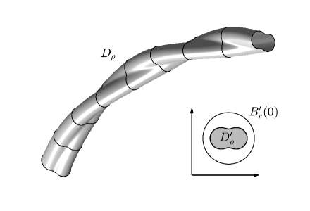
Figure 2.1: Sketch of the geometry of a thin nanowire $D_{\rho}$.

In the following, $\Gamma$ will be the spine curve of the nanowire. We restrict the discussion to thin nanowires with fixed but possibly twisting cross-section $D_{\rho}^{\prime}:=\rho B^{\prime}$, where the rescaled cross-section $B^{\prime}\subseteq B_{1}^{\prime}(0)\subseteq{\mathbb{R}}^{2}$ is a bounded Lipschitz domain. Here, $0<\rho<r$ is a scaling parameter that will determine the thickness of the nanowire. To describe the twisting of the cross-section of the nanowire along the spine curve, we let $\theta\in C^{2}([0,L],{\mathbb{R}})$ be a twisting function, and we define a two-dimensional parameter dependent rotation matrix

$$R_{\theta}(s)\,:=\,\begin{bmatrix}\cos\theta(s)&-\sin\theta(s)\\ \sin\theta(s)&\cos\theta(s)\end{bmatrix}\,,\qquad s\in[0,L]\,.$$ (2.3)

Accordingly, the support of the nanowire shall be given by

$$D_{\rho}\,:=\,\Bigl{\{}{\bm{X}}_{\bm{p}}(s,\eta,\xi)\;\Big{|}\;s\in[0,L]\,,\;R_{\theta}^{-1}(s)\begin{bmatrix}\eta\\ \xi\end{bmatrix}\in D_{\rho}^{\prime}\Bigr{\}}$$ (2.4)

(see Figure 2.1 for a sketch).

Remark 2.1.

In [11] we used the Frenet-Serret frame instead of a rotation minimizing frame to describe the geometry of thin tubular scattering objects as in (2.4). As a consequence, we had to assume that the spine curve $\Gamma$ has a non-vanishing curvature. Using a rotation minimizing frame, the analysis in [11] extends without further changes to spine curves, which may have vanishing curvature at some points. The special case, when $\Gamma$ is a straight line segment, has been considered in [8].  $\lozenge$

In contrast to the Frenet-Serret frame, the rotation minimizing frame $({\bm{t}}_{\bm{p}},{\bm{n}}_{\bm{p}},{\bm{b}}_{\bm{p}})$ in (2.2) is not uniquely determined. It depends on the particular choice of the reference vector ${\bm{n}}_{\bm{p}}(0)\perp{\bm{t}}_{\bm{p}}(0)$. A different reference vector requires a suitably modified twist function $\theta$ in (2.2) to obtain the same support $D_{\rho}$ for the nanowire in (2.4). To avoid this ambiguity, we use in the following a geometry adapted frame $({\bm{t}}_{\bm{p}},{\bm{n}}_{{\bm{p}},\theta},{\bm{b}}_{{\bm{p}},\theta})$, which is defined by

$$\bigl{[}{\bm{n}}_{{\bm{p}},\theta}(s)\big{|}{\bm{b}}_{{\bm{p}},\theta}(s)\bigr{]}\,:=\,\bigl{[}{\bm{n}}_{\bm{p}}(s)\big{|}{\bm{b}}_{\bm{p}}(s)\bigr{]}R_{\theta}(s)\,,\qquad s\in[0,L]\,.$$ (2.5)

Therewith,

$$D_{\rho}\,=\,\Bigl{\{}{\bm{p}}(s)+\eta\,{\bm{n}}_{{\bm{p}},\theta}(s)+\xi\,{\bm{b}}_{{\bm{p}},\theta}(s)\;\Big{|}\;s\in[0,L]\,,\;(\eta,\xi)\in D_{\rho}^{\prime}\Bigr{\}}.$$ (2.6)

This means that the twisting of the cross-section along the spine curve in the description of the support $D_{\rho}$ of the nanowire is now included into the frame. The twist rate $\beta:=\theta^{\prime}\in C([0,L],{\mathbb{R}})$ of the geometry adapted frame is defined by

$$\beta(s)\,=\,{\bm{n}}_{{\bm{p}},\theta}^{\prime}(s)\cdot{\bm{b}}_{{\bm{p}},\theta}(s)\,,\qquad s\in[0,L]\,.$$ (2.7)

We work with electric fields only, but the corresponding magnetic fields can immediately be obtained from the associated first order Maxwell systems. Let $\varepsilon_{0}:=8.85\times 10^{-12}$ Fm^-1 and ${\mu_{0}:=1.25\times 10^{-6}}$ Hm^-1 be the electric permittivity and the magnetic permeability of free space, respectively. Denoting by $f>0$ the frequency, the angular frequency is $\omega:=2\pi f$, and the associated wave number is given by $k:=\omega\sqrt{\varepsilon_{0}\mu_{0}}$. An electric incident field ${\bm{E}}^{i}$ is a solution to Maxwell’s equations

$$\operatorname{{\mathbf{curl}}}\operatorname{{\mathbf{curl}}}{\bm{E}}^{i}-k^{2}{\bm{E}}^{i}\,=\,0\qquad\text{in }{{\mathbb{R}}^{3}}\,.$$ (2.8)

		Silver			Gold
$f$		$\operatorname{Re}(\varepsilon_{r})$	$\operatorname{Im}(\varepsilon_{r})$		$\operatorname{Re}(\varepsilon_{r})$	$\operatorname{Im}(\varepsilon_{r})$
300 THz		-50.55	0.57		-41.78	2.94
350 THz		-36.23	0.48		-28.84	1.77
400 THz		-26.94	0.32		-20.11	1.24
450 THz		-20.57	0.44		-14.10	1.04
500 THz		-16.05	0.44		-9.36	1.53
550 THz		-12.62	0.42		-5.59	2.19
600 THz		-9.78	0.31		-2.54	3.65
650 THz		-7.64	0.25		-1.73	5.06
700 THz		-5.94	0.20		-1.69	5.66
750 THz		-4.41	0.21		-1.66	5.74
800 THz		-3.10	0.21		-1.50	5.63

Table 2.1: Relative electric permittivities $\varepsilon_{r}$ of silver and gold at optical frequencies (from [35]).

We suppose that the thin nanowire is made of a noble metal like silver or gold. At optical frequencies these materials are characterized by a frequency-dependent complex-valued relative electric permittivity $\varepsilon_{r}\in{\mathbb{C}}$ with negative real part $\operatorname{Re}(\varepsilon_{r})<0$ and positive imaginary part $\operatorname{Im}(\varepsilon_{r})>0$ (i.e., their electric permittivity is $\varepsilon_{m}:=\varepsilon_{0}\varepsilon_{r}$), while the magnetic permeability is the same as for the surrounding free space. The real and imaginary parts of the relative electric permittivities $\varepsilon_{r}$ of silver and gold at optical frequencies as considered in this work are retrieved from the data base [35]. They are shown in Table 2.1. We prefer these experimental data to the classical Drude model, because the Drude model is known to be rather inaccurate across the optical band (see e.g., [22, pp. 117–118]).

We denote by

$$\varepsilon_{\rho}\,:=\,\varepsilon_{0}+(\varepsilon_{m}-\varepsilon_{0})\chi_{D_{\rho}}$$ (2.9)

the piecewise constant electric permittivity distribution on ${{\mathbb{R}}^{3}}$ in the presence of the nanowire. Here, $\chi_{D_{\rho}}$ is the indicator function for $D_{\rho}$ from (2.4). The scattering problem consists in finding the total electric field ${\bm{E}}_{\rho}$ satisfying

$$\operatorname{{\mathbf{curl}}}\operatorname{{\mathbf{curl}}}{\bm{E}}_{\rho}-\omega^{2}\mu_{0}\varepsilon_{\rho}{\bm{E}}_{\rho}\,=\,0\qquad\text{in }{{\mathbb{R}}^{3}}\,,$$ (2.10a)

such that the scattered electric field

$${\bm{E}}^{s}_{\rho}\,:=\,{\bm{E}}_{\rho}-{\bm{E}}^{i}$$ (2.10b)

fulfills the Silver-Müller radiation condition

$$\lim_{|{\bm{x}}|\to\infty}\left(\operatorname{{\mathbf{curl}}}{\bm{E}}^{s}_{\rho}({\bm{x}})\times{\bm{x}}-\mathrm{i}k|{\bm{x}}|{\bm{E}}^{s}_{\rho}({\bm{x}})\right)\,=\,0$$ (2.10c)

uniformly with respect to all directions $\widehat{{\bm{x}}}:={\bm{x}}/|{\bm{x}}|\in{S^{2}}$.

Lemma 2.2.

Let $\varepsilon_{r}\in{\mathbb{C}}$ with $\operatorname{Re}(\varepsilon_{r})<0$ and $\operatorname{Im}(\varepsilon_{r})>0$, and let $D_{\rho}\subseteq{{\mathbb{R}}^{3}}$ and $\varepsilon_{\rho}$ be as in (2.4) and (2.9) for some $0<\rho<r$, respectively. Suppose that ${\bm{E}}^{i}\in H_{{\mathrm{loc}}}(\operatorname{{\mathbf{curl}}};{\mathbb{R}}^{3})$ satisfies (2.8). Then, the scattering problem (2.10) has a unique solution ${\bm{E}}_{\rho}\in H_{{\mathrm{loc}}}(\operatorname{{\mathbf{curl}}};{{\mathbb{R}}^{3}})$. The corresponding scattered electric field ${\bm{E}}^{s}_{\rho}$ has the asymptotic behavior

$${\bm{E}}^{s}_{\rho}({\bm{x}})\,=\,\frac{\mathrm{e}^{\mathrm{i}k|{\bm{x}}|}}{4\pi|{\bm{x}}|}\left({\bm{E}}^{\infty}_{\rho}(\widehat{{\bm{x}}})+\mathcal{O}(|{\bm{x}}|^{-1})\right)\qquad\text{as }|{\bm{x}}|\to\infty$$

uniformly in $\widehat{{\bm{x}}}\in{S^{2}}$. The vector function ${\bm{E}}^{\infty}_{\rho}\in{L^{2}_{t}(S^{2},{{\mathbb{C}}^{3}})}$ is called the electric far field pattern.

Proof.

The uniqueness of solutions follows exactly as in the proof of [40, Thm. 10.1], where complex electric permittivities with positive real and imaginary parts have been considered. The existence of solutions can be obtained applying Riesz-Fredholm theory, using the same arguments as in [40, Sect. 10.3]. The far field expansion has been shown in [40, Cor. 9.5]. ∎

We focus on thin metallic nanowires, i.e., the scaling parameter $0<\delta<r$ in (2.4) is supposed to be small relative to the wave length $\lambda=2\pi/k$ and relative to the total length $L$ of the nanowire. In this case, solutions to the scattering problem (2.10) can be accurately described by the following asymptotic representation formula.

Theorem 2.3.

Let $\varepsilon_{r}\in{\mathbb{C}}$ with $\operatorname{Re}(\varepsilon_{r})<0$ and $\operatorname{Im}(\varepsilon_{r})>0$, and for any $0<\rho<r$ let $D_{\rho}\subseteq{{\mathbb{R}}^{3}}$ and $\varepsilon_{\rho}$ be as in (2.4) and (2.9), respectively. Denoting by ${\bm{E}}^{i}$ an electric incident field, the electric far field pattern corresponding to the solution of the scattering problem (2.10) satisfies, for each $\widehat{{\bm{x}}}\in{S^{2}}$,

$$\begin{split}{\bm{E}}^{\infty}_{\rho}(\widehat{{\bm{x}}})&\,=\,|B^{\prime}|(k\rho)^{2}\int_{\Gamma}(\varepsilon_{r}-1)\mathrm{e}^{-\mathrm{i}k\widehat{{\bm{x}}}\cdot{\bm{y}}}\bigl{(}(\widehat{{\bm{x}}}\times\mathbb{I}_{3})\times\widehat{{\bm{x}}}\bigr{)}\mathbb{M}^{\varepsilon}({\bm{y}}){\bm{E}}^{i}({\bm{y}})\,\operatorname{d\!}s({\bm{y}})+o\bigl{(}(k\rho)^{2}\bigr{)}\end{split}$$ (2.11)

as $\rho\to 0$. Here, $|B^{\prime}|$ denotes the area of the rescaled cross-section $B^{\prime}=D_{\rho}^{\prime}/\rho$, $\mathbb{I}_{3}\in{{\mathbb{R}}^{3\times 3}}$ is the identity matrix, and the matrix valued function $\mathbb{M}^{\varepsilon}\in L^{2}(\Gamma,{{\mathbb{C}}^{3\times 3}})$ is the electric polarization tensor. The term $o((k\rho)^{2})$ in (2.11) is such that $\|o((k\rho)^{2})\|_{L^{\infty}({S^{2}})}/(k\rho)^{2}$ converges to zero for any fixed ${\bm{E}}^{i}$ satisfying $\|{\bm{E}}^{i}\|_{H(\operatorname{{\mathbf{curl}}};{B_{R}(0)})}\leq C$ for some fixed $C>0$.

Theorem 2.3 is a special case of a more general result that has been established for scatterers of low volume with complex electric permittivities with positive real and nonnegative imaginary part in [1, 11, 25] (see also [12] for an earlier version of this asymptotic perturbation formula in electrostatics). Using the well-posedness from Lemma 2.2, this result including its proof carries over to the case of metallic nanowires with complex electric permittivities with negative real and positive imaginary part as considered in this work.

The electric polarization tensor $\mathbb{M}^{\varepsilon}\in L^{2}(\Gamma,{{\mathbb{C}}^{3\times 3}})$ in (2.11) is defined as follows (see [11, 25]). Let $R>0$ be sufficiently large such that ${D_{\rho}\subset\subset{B_{R}(0)}}$ for all $0<\rho<r$. For any $\bm{\xi}\in{S^{2}}$, we denote by ${W_{\rho}^{(\bm{\xi})}\in H^{1}({B_{R}(0)})}$ the corrector potentials satisfying

$$\mathrm{div}\bigl{(}\varepsilon_{\rho}\nabla W_{\rho}^{(\bm{\xi})}\bigr{)}\,=\,-\mathrm{div}\bigl{(}(\varepsilon_{\rho}-\varepsilon_{0})\bm{\xi}\bigr{)}\quad\text{in ${B_{R}(0)}$}\,,\qquad W_{\rho}^{(\bm{\xi})}\,=\,0\quad\text{on $\partial{B_{R}(0)}$}\,.$$ (2.12)

Then, the electric polarization tensor is uniquely determined by

$$\frac{1}{|\Gamma|}\int_{\Gamma}\bm{\xi}\cdot\mathbb{M}^{\varepsilon}\bm{\xi}\psi\,\operatorname{d\!}s\,=\,\frac{1}{|D_{\rho}|}\int_{D_{\rho}}|\bm{\xi}|^{2}\psi\,\operatorname{d\!}{\bm{x}}+\frac{1}{|D_{\rho}|}\int_{D_{\rho}}\bigl{(}\bm{\xi}\cdot\nabla W_{\rho}^{(\bm{\xi})}\bigr{)}\psi\,\operatorname{d\!}{\bm{x}}+o(1)\qquad\text{as }\rho\to 0$$ (2.13)

for all $\psi\in C(\overline{{B_{R}(0)}})$ and any $\bm{\xi}\in{S^{2}}$. In contrast to the very general situation considered in [11, Thm. 1], no extraction of a subsequence is required in (2.13) under our assumptions on the geometry of the cross-sections (see [11, Rem. 4.5]).

Remark 2.4 (Dielectric nanowires).

For dielectric nanowires, i.e., when $\varepsilon_{r}>0$ is positive, the electric polarization tensor $\mathbb{M}^{\varepsilon}\in L^{2}(\Gamma,{{\mathbb{R}}^{3\times 3}})$ is a real-valued, symmetric, and positive definite matrix pointwise a.e. on $\Gamma$ (see [12, Sec. 4]). In particular, it can be diagonalized. A pointwise characterization of the eigenvalues and eigenvectors of $\mathbb{M}^{\varepsilon}$ has been established in [11, Thm. 4.1] (see [8] for the special case when $\Gamma$ is a straight line segment). It has been shown that, for a.e. $s\in[0,L]$, the tangent vector ${\bm{t}}_{\bm{p}}(s)$ is an eigenvector of the electric polarization tensor $\mathbb{M}^{\varepsilon}({\bm{p}}(s))$ corresponding to the eigenvalue $1$. Furthermore, using the vectors $({\bm{n}}_{{\bm{p}},\theta}(s),{\bm{b}}_{{\bm{p}},\theta}(s))$ from (2.5) as a basis of the plane orthogonal to ${\bm{t}}_{\bm{p}}(s)$, the electric polarization tensor reduces to the corresponding two-dimensional electric polarization tensor $\mathbbm{m}^{\varepsilon}$ associated to the rescaled cross-sections $B^{\prime}=D_{\rho}^{\prime}/\rho$ in this plane. Here, $\mathbbm{m}^{\varepsilon}=(\mathbbm{m}^{\varepsilon}_{ij})\in{\mathbb{C}}^{2\times 2}$ is given by

$$\mathbbm{m}^{\varepsilon}_{ij}\,=\,\delta_{ij}+\frac{1}{|B^{\prime}|}\int_{B^{\prime}}\frac{\partial w_{j}}{\partial x^{\prime}_{i}}({\bm{x}}^{\prime})\,\operatorname{d\!}{\bm{x}}^{\prime}\,,\qquad 1\leq i,j\leq 2\,,$$ (2.14)

where $\delta_{ij}$ denotes the Kronecker delta, and $w_{j}\in H^{1}_{\mathrm{loc}}({\mathbb{R}}^{2})$ is the unique solution to the transmission problem

$$\Delta w_{j} \,=\,0\qquad\quad\text{in }{\mathbb{R}}^{2}\setminus\partial B^{\prime}\,,$$ (2.15a)

$$w_{j}\big{|}_{\partial B^{\prime}}^{+}-w_{j}\big{|}_{\partial B^{\prime}}^{-} \,=\,0\,,$$ (2.15b)

$$\frac{\partial w_{j}}{\partial{\bm{\nu}}}\Big{|}_{\partial B^{\prime}}^{+}-\varepsilon_{r}\frac{\partial w_{j}}{\partial{\bm{\nu}}}\Big{|}_{\partial B^{\prime}}^{-} \,=\,(\varepsilon_{r}-1)\nu_{j}\,,$$ (2.15c)

$$w_{j}({\bm{x}}^{\prime}) \to 0\qquad\quad\text{as $|{\bm{x}}^{\prime}|\to\infty$}\,.$$ (2.15d)

(see [11, Rem 4.5]). Given any specific geometry for $B^{\prime}$, the functions $w_{j}$, $j=1,2$, in (2.14) can be approximated by solving the two-dimensional transmission problem (2.15) numerically. Then, the two-dimensional electric polarization tensor $\mathbbm{m}^{\varepsilon}$ can be evaluated by applying a quadrature rule to the integral in (2.14). In the special case when $B^{\prime}$ is an ellipse with semi axes of lengths $a$ and $b$ for some $0<a\leq b<1$ that are aligned with the coordinate axes in ${{\mathbb{R}}^{2}}$, the transmission problem (2.15) can be solved by separation of variables. Then, the integral in (2.14) can be evaluated explicitly to obtain that

$$\mathbbm{m}^{\varepsilon}\,=\,\begin{bmatrix}\frac{a+b}{a+\varepsilon_{r}b}&0\\ 0&\frac{a+b}{b+\varepsilon_{r}a}\end{bmatrix}$$ (2.16)

(see, e.g., [5, 10]). Here, the semi axis of length $a$ is aligned with the $x_{1}$-axis and the semi axis of length $b$ is aligned with the $x_{2}$-axis.  $\lozenge$

When $\varepsilon_{r}$ is complex-valued with negative real and positive imaginary part, the electric polarization tensor $\mathbb{M}^{\varepsilon}\in L^{2}(\Gamma,{{\mathbb{C}}^{3\times 3}})$ is still symmetric pointwise a.e. on $\Gamma$ (see Lemma A.1 in the appendix), but this no longer implies diagonalizability. However, the following statements of [11, Thm. 4.1] including their proofs remain valid for such complex-valued relative electric permittivities.

Proposition 2.5.

Suppose $\varepsilon_{r}\in{\mathbb{C}}$ with $\operatorname{Re}(\varepsilon_{r})<0$ and $\operatorname{Im}(\varepsilon_{r})>0$, and for any $0<\rho<r$ let $D_{\rho}\subseteq{{\mathbb{R}}^{3}}$ and $\varepsilon_{\rho}$ be as in (2.4) and (2.9), respectively. Let $\mathbb{M}^{\varepsilon}\in L^{2}(\Gamma,{{\mathbb{C}}^{3\times 3}})$ be the electric polarization tensor defined in (2.12)–(2.13) and denote by $\mathbbm{m}^{\varepsilon}\in{\mathbb{C}}^{2\times 2}$ the polarization tensor corresponding to the rescaled cross-section $B^{\prime}=D_{\rho}^{\prime}/\rho$ defined in (2.14)–(2.15). Then, the following pointwise characterization of $\mathbb{M}^{\varepsilon}$ holds.

1. Let ${\bm{t}}_{\bm{p}}(s)$ be the unit tangent vector at ${\bm{p}}(s)\in\Gamma$, then

   $${\bm{t}}_{\bm{p}}(s)\cdot\mathbb{M}^{\varepsilon}({\bm{p}}(s)){\bm{t}}_{\bm{p}}(s)\,=\,1\qquad\text{for a.e.\ $s\in[0,L]$}\,.$$ (2.17)

2. Let $({\bm{n}}_{{\bm{p}},\theta},{\bm{b}}_{{\bm{p}},\theta})$ be the normal components of the geometry adapted frame $({\bm{t}}_{\bm{p}},{\bm{n}}_{{\bm{p}},\theta},{\bm{b}}_{{\bm{p}},\theta})$ from (2.5), let $\bm{\xi}^{\prime}\in{S^{1}}$, and let $\bm{\xi}\in C^{1}([0,L],{S^{2}})$ be given by $\bm{\xi}(s):=\bigl{[}{\bm{n}}_{{\bm{p}},\theta}(s),{\bm{b}}_{{\bm{p}},\theta}(s)\bigr{]}\bm{\xi}^{\prime}\in{S^{2}}$ for all ${s\in[0,L]}$. Then,

   $$\bm{\xi}(s)\cdot\mathbb{M}^{\varepsilon}({\bm{p}}(s))\bm{\xi}(s)\,=\,\bm{\xi}^{\prime}\cdot\mathbbm{m}^{\varepsilon}\bm{\xi}^{\prime}\qquad\text{for a.e.\ $s\in[0,L]$}\,.$$

As in the dielectric case, we use pointwise polarization tensor bounds to show that the unit tangent vector ${\bm{t}}_{\bm{p}}(s)$ is in fact an eigenvector of $\mathbb{M}^{\varepsilon}({\bm{p}}(s))$ corresponding to the eigenvalue $1$ for a.e. $s\in[0,L]$. These bounds, which are different from the corresponding polarization tensor bounds in the dielectric case from [12], are shown in Lemma A.1 in the appendix.

Lemma 2.6.

Suppose $\varepsilon_{r}\in{\mathbb{C}}$ with $\operatorname{Re}(\varepsilon_{r})<0$ and $\operatorname{Im}(\varepsilon_{r})>0$, and for any $0<\rho<r$ let $D_{\rho}\subseteq{{\mathbb{R}}^{3}}$ and $\varepsilon_{\rho}$ be as in (2.4) and (2.9), respectively. Let $\mathbb{M}^{\varepsilon}\in L^{2}(\Gamma,{{\mathbb{C}}^{3\times 3}})$ be the electric polarization tensor defined in (2.12)–(2.13). Then, the unit tangent vector ${\bm{t}}_{\bm{p}}(s)$ is an eigenvector of the matrix $\mathbb{M}^{\varepsilon}({\bm{p}}(s))$ corresponding to the eigenvalue $1$ for a.e. $s\in[0,L]$.

Proof.

From Lemma A.1 in the appendix we obtain that there exists $\gamma\in(0,\pi/2)$ such that $\operatorname{Re}(\mathrm{e}^{\mathrm{i}\gamma}\overline{\varepsilon_{0}})>0$, $\operatorname{Re}(\mathrm{e}^{\mathrm{i}\gamma}\overline{\varepsilon_{m}})>0$, and $\operatorname{Re}(\mathrm{e}^{\mathrm{i}\gamma}(\overline{\varepsilon_{m}-\varepsilon_{0}}))<0$. Observing that, for any $\bm{\xi}\in{S^{2}}$,

$$\bm{\xi}\cdot\operatorname{Re}\left(\mathrm{e}^{\mathrm{i}\gamma}(\overline{\varepsilon_{m}-\varepsilon_{0}})\mathbb{M}^{\varepsilon}\right)\bm{\xi} \,=\,\bm{\xi}\cdot\left(\operatorname{Re}\left(\mathrm{e}^{\mathrm{i}\gamma}(\overline{\varepsilon_{m}-\varepsilon_{0}})\right)\operatorname{Re}(\mathbb{M}^{\varepsilon})-\operatorname{Im}\left(\mathrm{e}^{\mathrm{i}\gamma}(\overline{\varepsilon_{m}-\varepsilon_{0}})\right)\operatorname{Im}(\mathbb{M}^{\varepsilon})\right)\bm{\xi}\,,$$ (2.18a)

$$\bm{\xi}\cdot\operatorname{Im}\left((\overline{\varepsilon_{m}-\varepsilon_{0}})\mathbb{M}^{\varepsilon}\right)\bm{\xi} \,=\,\bm{\xi}\cdot\left(\operatorname{Re}\left((\overline{\varepsilon_{m}-\varepsilon_{0}})\right)\operatorname{Im}(\mathbb{M}^{\varepsilon})+\operatorname{Im}\left((\overline{\varepsilon_{m}-\varepsilon_{0}})\right)\operatorname{Re}(\mathbb{M}^{\varepsilon})\right)\bm{\xi}\,,$$ (2.18b)

the inequality (A.5) can be rewritten as

$$|\bm{\xi}|^{2}\,\leq\,\bm{\xi}\cdot\left(\operatorname{Re}(\mathbb{M}^{\varepsilon}({\bm{x}}))-\frac{\operatorname{Im}\left(\mathrm{e}^{\mathrm{i}\gamma}(\overline{\varepsilon_{m}-\varepsilon_{0}})\right)}{\operatorname{Re}\left(\mathrm{e}^{\mathrm{i}\gamma}(\overline{\varepsilon_{m}-\varepsilon_{0}})\right)}\operatorname{Im}(\mathbb{M}^{\varepsilon}({\bm{x}}))\right)\bm{\xi}\qquad\text{for every }\bm{\xi}\in{S^{2}}\text{ and a.e.\ }{\bm{x}}\in\Gamma\,.$$ (2.19)

Moreover, subtracting (A.5) from (A.4) and using (2.18) gives that

$$\bm{\xi}\cdot\left(\frac{\operatorname{Re}(\overline{\varepsilon_{m}-\varepsilon_{0}})}{\operatorname{Im}(\overline{\varepsilon_{m}-\varepsilon_{0}})}+\frac{\operatorname{Im}(\mathrm{e}^{\mathrm{i}\gamma}(\overline{\varepsilon_{m}-\varepsilon_{0}}))}{\operatorname{Re}(\mathrm{e}^{\mathrm{i}\gamma}(\overline{\varepsilon_{m}-\varepsilon_{0}}))}\right)\operatorname{Im}(\mathbb{M}^{\varepsilon}({\bm{x}}))\bm{\xi}\,\leq\,0\qquad\text{for every }\bm{\xi}\in{S^{2}}\text{ and a.e.\ }{\bm{x}}\in\Gamma\,.$$ (2.20)

Since the real factor on the left hand side of (2.20) is strictly positive by our assumptions on $\varepsilon_{r}$ and $\gamma$, this implies that

$$\bm{\xi}\cdot\operatorname{Im}(\mathbb{M}^{\varepsilon}({\bm{x}}))\bm{\xi}\,\leq\,0\qquad\text{for every }\bm{\xi}\in{S^{2}}\text{ and a.e.\ }{\bm{x}}\in\Gamma\,.$$ (2.21)

Now, considering the imaginary part of (2.17), applying the min-max principle and using (2.21), we find that the tangent vector ${\bm{t}}_{\bm{p}}(s)$ is an eigenvector of the self-adjoint matrix $\operatorname{Im}(\mathbb{M}^{\varepsilon}({\bm{p}}(s)))$ corresponding to the eigenvalue $0$ for a.e. $s\in[0,L]$. Similarly, considering the real part of (2.17), applying the min-max principle and using (2.19), shows that ${\bm{t}}_{\bm{p}}(s)$ is an eigenvector of the self-adjoint matrix $\operatorname{Re}(\mathbb{M}^{\varepsilon}({\bm{p}}(s)))$ corresponding to the eigenvalue $1$ for a.e. $s\in[0,L]$. Since $\mathbb{M}^{\varepsilon}=\operatorname{Re}(\mathbb{M}^{\varepsilon})+\mathrm{i}\operatorname{Im}(\mathbb{M}^{\varepsilon})$, this ends the proof. ∎

Combining Proposition 2.5 and Lemma 2.6 shows that the electric polarization tensor $\mathbb{M}^{\varepsilon}\in L^{2}(\Gamma,{{\mathbb{C}}^{3\times 3}})$ in the asymptotic representation formula (2.11) satisfies

$$\mathbb{M}^{\varepsilon}({\bm{p}}(s))\,=\,V_{{\bm{p}},\theta}(s)M^{\varepsilon}V_{{\bm{p}},\theta}^{\top}(s)\quad\text{for a.e.\ }s\in[0,L]\,,$$ (2.22a)

where the matrix valued function $$V_{{\bm{p}},\theta}\in C^{1}([0,L],\mathrm{SO}(3)) V_{{\bm{p}},\theta}:=[{\bm{t}}_{\bm{p}}|{\bm{n}}_{{\bm{p}},\theta}|{\bm{b}}_{{\bm{p}},\theta}]$$ is given by , and

$$M^{\varepsilon}\,:=\,\begin{bmatrix}1&\vline&\begin{matrix}0&0\end{matrix}\\ \hline\cr\begin{matrix}0\\ 0\end{matrix}&\vline&\mathbbm{m}^{\varepsilon}\end{bmatrix}\in{{\mathbb{C}}^{3\times 3}}\,.$$ (2.22b)

Therewith, the asymptotic representation formula (2.11) yields an efficient tool to evaluate the electric far field pattern due to a thin metallic nanowire.

Remark 2.7 (Plasmonic resonances).

In the special case, when the reference cross-section $B^{\prime}$ is an ellipse with semi axes of length $0<a\leq b<1$, we observe from (2.22) and (2.16) that the norm of the polarization tensor is large, when either $\varepsilon_{r}\approx-a/b$ or $\varepsilon_{r}\approx-b/a$. For noble metals like silver or gold, $\operatorname{Im}(\varepsilon_{r})>0$ is strictly positive, and therefore the polarization tensor does not become singular for any choice of $a/b$ (see Table 2.1 for the relative electric permittivity $\varepsilon_{r}$ of silver and gold at optical frequencies). However, according to (2.11) strong scattering occurs, whenever $\operatorname{Im}(\varepsilon_{r})$ is small and $\operatorname{Re}(\varepsilon_{r})=-a/b$ or $\operatorname{Re}(\varepsilon_{r})=-b/a$. Following [3] (see also [23, 41]) we call the corresponding frequencies $f_{\mathrm{res}}$ plasmonic resonances for $D_{\rho}$.

Since $\operatorname{Re}(\varepsilon_{r})<-1$ for silver and gold across the optical band (see Table 2.1), and $0<a\leq b<1$ by assumption, i.e., $-\infty<-b/a\leq-1\leq-a/b\leq 0$, only the plasmonic resonance $f_{\mathrm{res}}$ with $\operatorname{Re}(\varepsilon_{r}(f_{\mathrm{res}}))=-b/a$ can be excited for silver and gold nanowires with elliptical cross-sections at optical frequencies.

For general cross-sections $D_{\rho}^{\prime}$, plasmonic resonances can be determined by solving an eigenvalue problem for the Neumann-Poincáre operator on the boundary of the rescaled cross-section $B^{\prime}=D_{\rho}^{\prime}/\rho$ (see [3]). The optimal design of two-dimensional shapes that resonate at particular frequencies has been considered in [2].  $\lozenge$

3 Electromagnetic chirality

In this section we briefly summarize the concept of electromagnetic chirality. For further details we refer to [7, 16, 45]. An electric plane wave with direction of propagation ${\bm{\theta}}\in{S^{2}}$ and polarization ${\bm{A}}\in{\mathbb{C}}^{3}$, which must satisfy ${\bm{A}}\cdot{\bm{\theta}}=0$, is described by the matrix ${\bm{E}}^{i}(\,\cdot\,;{\bm{\theta}})\in{{\mathbb{C}}^{3\times 3}}$ defined by

$${\bm{E}}^{i}({\bm{x}};{\bm{\theta}}){\bm{A}}\,=\,{\bm{A}}\,\mathrm{e}^{\mathrm{i}k{\bm{\theta}}\cdot{\bm{x}}}\,,\qquad{\bm{x}}\in{{\mathbb{R}}^{3}}\,,$$

We consider scattering of an electric plane wave at a thin nanowire $D_{\rho}$ with relative electric permittivity $\varepsilon_{r}$. Because of the linearity of (2.10) with respect to the incident field, we can also express the scattered electric field and the electric far field pattern by matrices ${\bm{E}}^{s}_{\rho}(\,\cdot\,;{\bm{\theta}})$ and ${\bm{E}}^{\infty}_{\rho}(\,\cdot\,;{\bm{\theta}})$, respectively. Accordingly, the scattered field associated to an electric Herglotz incident wave

$${\bm{E}}^{i}[{\bm{A}}]({\bm{x}})\,:=\,\int_{{S^{2}}}{\bm{A}}({\bm{\theta}})\mathrm{e}^{\mathrm{i}k{\bm{\theta}}\cdot{\bm{x}}}\,\operatorname{d\!}s({\bm{\theta}})\,,\qquad{\bm{x}}\in{{\mathbb{R}}^{3}}\,,$$ (3.1)

with density ${\bm{A}}\in{L^{2}_{t}(S^{2},{{\mathbb{C}}^{3}})}$ is given by

$${\bm{E}}^{s}_{\rho}[{\bm{A}}]({\bm{x}})\,=\,\int_{{S^{2}}}{\bm{E}}^{s}_{\rho}({\bm{x}};{\bm{\theta}}){\bm{A}}({\bm{d}})\,\operatorname{d\!}s({\bm{d}})\,,\qquad{\bm{x}}\in{{\mathbb{R}}^{3}}\,.$$

The electric far field operator $\mathcal{F}_{D_{\rho}}:{L^{2}_{t}(S^{2},{{\mathbb{C}}^{3}})}\to{L^{2}_{t}(S^{2},{{\mathbb{C}}^{3}})}$,

$$(\mathcal{F}_{D_{\rho}}{\bm{A}})(\widehat{{\bm{x}}})\,:=\,{\bm{E}}^{\infty}_{\rho}[{\bm{A}}](\widehat{{\bm{x}}})\,=\,\int_{{S^{2}}}{\bm{E}}^{\infty}_{\rho}(\widehat{{\bm{x}}};{\bm{\theta}}){\bm{A}}({\bm{\theta}})\,\operatorname{d\!}s({\bm{\theta}})\,,\qquad\widehat{{\bm{x}}}\in{S^{2}}\,,$$

maps densities of electric Herglotz incident waves to the far field patterns of the corresponding scattered electric fields. Since the kernel of this integral operator is smooth, it is compact and of Hilbert-Schmidt class, i.e., $\mathcal{F}_{D_{\rho}}\in\mathrm{HS}({L^{2}_{t}(S^{2},{{\mathbb{C}}^{3}})})$.

Electromagnetic chirality describes different responses of scattering objects to electromagnetic fields of positive and negative helicities. An electric field ${\bm{E}}^{i}$, ${\bm{E}}_{\rho}$, or ${\bm{E}}^{s}_{\rho}$ in ${{\mathbb{R}}^{3}}\setminus\overline{D_{\rho}}$ is said to have helicity $\pm 1$ if it is an eigenfunction of the operator $k^{-1}\operatorname{{\mathbf{curl}}}$ associated to the eigenvalue $\pm 1$. Using the Riemann-Silberstein combinations ${\bm{U}}\pm k^{-1}\operatorname{{\mathbf{curl}}}{\bm{U}}$, any solution to $\operatorname{{\mathbf{curl}}}\operatorname{{\mathbf{curl}}}{\bm{U}}-k^{2}{\bm{U}}=0$ in some subdomain of ${{\mathbb{R}}^{3}}$ can be decomposed into a sum of two fields of helicity $+1$ and $-1$. The helicity of an electric Herglotz wave ${\bm{E}}^{i}[{\bm{A}}]$ and of the corresponding scattered electric field ${\bm{E}}^{s}_{\rho}[{\bm{A}}]|_{{{\mathbb{R}}^{3}}\setminus\overline{D_{\rho}}}$ is uniquely determined by the density ${\bm{A}}$ and by the associated far field pattern ${\bm{E}}^{\infty}_{\rho}[{\bm{A}}]$, respectively. Decomposing ${L^{2}_{t}(S^{2},{{\mathbb{C}}^{3}})}=V^{+}\oplus V^{-}$ into the two orthogonal eigenspaces

$$V^{\pm}\,:=\,\{{\bm{A}}\pm\mathcal{C}{\bm{A}}\;|\;{\bm{A}}\in{L^{2}_{t}(S^{2},{{\mathbb{C}}^{3}})}\}$$ (3.2)

of the self-adjoint linear operator $\mathcal{C}:{L^{2}_{t}(S^{2},{{\mathbb{C}}^{3}})}\to{L^{2}_{t}(S^{2},{{\mathbb{C}}^{3}})}$,

$$(\mathcal{C}{\bm{A}})({\bm{\theta}})\,:=\,\mathrm{i}{\bm{\theta}}\times{\bm{A}}({\bm{\theta}})\,,\qquad{\bm{\theta}}\in{S^{2}}\,,$$

it has been shown in [7, 16] that

$${\bm{E}}^{i}[{\bm{A}}]\,\text{ has helicity }\pm 1 \qquad\text{if and only if}\qquad{\bm{A}}\in V^{\pm}\,,$$

$${\bm{E}}^{s}_{\rho}[{\bm{A}}]|_{{{\mathbb{R}}^{3}}\setminus\overline{D_{\rho}}}\,\text{ has helicity }\pm 1 \qquad\text{if and only if}\qquad\mathcal{F}_{D_{\rho}}{\bm{A}}\in V^{\pm}\,.$$

Using the orthogonal projections $\mathcal{P}^{\pm}:{L^{2}_{t}(S^{2},{{\mathbb{C}}^{3}})}\to{L^{2}_{t}(S^{2},{{\mathbb{C}}^{3}})}$ onto $V^{\pm}$, we define the projected far field operators $\mathcal{F}_{D_{\rho}}^{cd}:=\mathcal{P}^{c}\mathcal{F}_{D_{\rho}}\mathcal{P}^{d}$ for $c,d\in\{+,-\}$. Then, $\mathcal{F}_{D_{\rho}}^{cd}$ describes the components with helicity $c$ of all possible electric far field patterns corresponding to electric Herglotz incident waves with helicity $d$. Therewith, the far field operator $\mathcal{F}_{D_{\rho}}$ can be decomposed into four blocks

$$\mathcal{F}_{D_{\rho}}\,=\,\mathcal{F}_{D_{\rho}}^{++}+\mathcal{F}_{D_{\rho}}^{+-}+\mathcal{F}_{D_{\rho}}^{-+}+\mathcal{F}_{D_{\rho}}^{--}\,.$$ (3.3)

The following notion of electromagnetic chirality has been introduced in [16] (see also [7]). Roughly speaking, the idea is to decide whether the information content of the electric far field patterns corresponding to all possible electric incident fields with positive helicity can be reproduced using all possible electric incident fields of negative helicity and vice versa, or not.

Definition 3.1.

A scatterer $D_{\rho}$ is electromagnetically achiral (or em-achiral) if there exist unitary operators $\mathcal{U}^{(j)}:{L^{2}_{t}(S^{2},{{\mathbb{C}}^{3}})}\to{L^{2}_{t}(S^{2},{{\mathbb{C}}^{3}})}$ satisfying $\mathcal{U}^{(j)}\mathcal{C}=-\mathcal{C}\mathcal{U}^{(j)}$, $j=1,\ldots,4$, such that

$$\mathcal{F}_{D_{\rho}}^{++}\,=\,\mathcal{U}^{(1)}\mathcal{F}_{D_{\rho}}^{--}\mathcal{U}^{(2)}\,,\qquad\mathcal{F}_{D_{\rho}}^{-+}\,=\,\mathcal{U}^{(3)}\mathcal{F}_{D_{\rho}}^{+-}\mathcal{U}^{(4)}\,.$$

If this is not the case, then the scatterer $D_{\rho}$ is electromagnetically chiral (or em-chiral).

For $c,d\in\{+,-\}$ let $(\sigma_{j}^{cd})_{j\in{\mathbb{N}}}$ denote the singular values of $\mathcal{F}_{D_{\rho}}^{cd}$ in decreasing order and repeated with multiplicity. Then, Definition 3.1 says that a scattering object $D_{\rho}$ is em-achiral if and only if

$$(\sigma_{j}^{++})_{j\in{\mathbb{N}}}\,=\,(\sigma_{j}^{--})_{j\in{\mathbb{N}}}\qquad\text{and}\qquad(\sigma_{j}^{+-})_{j\in{\mathbb{N}}}\,=\,(\sigma_{j}^{-+})_{j\in{\mathbb{N}}}\,.$$

Accordingly, it has been proposed in [16] to quantify the degree of em-chirality of a scattering object by means of the distance of the corresponding sequences of singular values. In this work, we discuss two possible choices for such an em-chirality measure of a scatterer $D_{\rho}$ with associated far field operator $\mathcal{F}_{D_{\rho}}$. The measure $\chi_{2}$ from [16], which is defined by

$$\chi_{2}(\mathcal{F}_{D_{\rho}})\,:=\,\Bigl{(}\bigl{\|}(\sigma_{j}^{++})_{j\in{\mathbb{N}}}-(\sigma_{j}^{--})_{j\in{\mathbb{N}}}\bigr{\|}_{\ell^{2}}^{2}+\bigl{\|}(\sigma_{j}^{+-})_{j\in{\mathbb{N}}}-(\sigma_{j}^{-+})_{j\in{\mathbb{N}}}\bigr{\|}_{\ell^{2}}^{2}\Bigr{)}^{\frac{1}{2}}\,,$$ (3.4a)

and a smooth relaxation $$\chi_{\mathrm{HS}} \chi_{2}$$ of from [29], which is given by

$$\chi_{\mathrm{HS}}(\mathcal{F}_{D_{\rho}})\,:=\,\bigl{(}\bigl{(}\|\mathcal{F}_{D_{\rho}}^{++}\|_{\mathrm{HS}}-\|\mathcal{F}_{D_{\rho}}^{--}\|_{\mathrm{HS}}\bigr{)}^{2}+\bigl{(}\|\mathcal{F}_{D_{\rho}}^{-+}\|_{\mathrm{HS}}-\|\mathcal{F}_{D_{\rho}}^{+-}\|_{\mathrm{HS}}\bigr{)}^{2}\bigr{)}^{\frac{1}{2}}\,.$$ (3.4b)

Here, $\|\,\cdot\,\|_{\mathrm{HS}}$ denotes the Hilbert-Schmidt norm. The Hilbert-Schmidt norm $\|\mathcal{F}_{D_{\rho}}\|_{\mathrm{HS}}$ of the far field operator $\mathcal{F}_{D_{\rho}}$ is sometimes called the total interaction cross section of the scattering object $D_{\rho}$. It has been shown in [7, 16, 29] that

$$0\,\leq\,\chi_{\mathrm{HS}}(\mathcal{F}_{D_{\rho}})\,\leq\,\chi_{2}(\mathcal{F}_{D_{\rho}})\,\leq\,\|\mathcal{F}_{D_{\rho}}\|_{\mathrm{HS}}\,.$$ (3.5)

For the lower and upper bounds in (3.5) we have that

$$\chi_{\mathrm{HS}}(\mathcal{F}_{D_{\rho}}) \,=\,0\phantom{\|\mathcal{F}_{D_{\rho}}\|_{\mathrm{HS}}}\;\quad\text{if and only if}\qquad\chi_{2}(\mathcal{F}_{D_{\rho}})\,=\,0\,,$$

$$\chi_{\mathrm{HS}}(\mathcal{F}_{D_{\rho}}) \,=\,\|\mathcal{F}_{D_{\rho}}\|_{\mathrm{HS}}\phantom{0}\;\quad\text{if and only if}\qquad\chi_{2}(\mathcal{F}_{D_{\rho}})\,=\,\|\mathcal{F}_{D_{\rho}}\|_{\mathrm{HS}}\,.$$

The scatterer $D_{\rho}$ is em-achiral if and only if $\chi_{2}(\mathcal{F}_{D_{\rho}})=\chi_{\mathrm{HS}}(\mathcal{F}_{D_{\rho}})=0$, and it is said to be maximally em-chiral if $\chi_{2}(\mathcal{F}_{D_{\rho}})=\chi_{\mathrm{HS}}(\mathcal{F}_{D_{\rho}})=\|\mathcal{F}_{D_{\rho}}\|_{\mathrm{HS}}$. The latter is equivalent to the fact that the scatterer $D_{\rho}$ does not scatter incident fields of either positive or negative helicity at all.

4 Optimal shape design

We consider the shape optimization problem to design thin metallic nanowires that are as close to being maximally em-chiral at optical frequencies as possible. To this end, we maximize the normalized em-chirality measures $\chi_{2}(\mathcal{F}_{D_{\rho}})/\|\mathcal{F}_{D_{\rho}}\|_{\mathrm{HS}}$ and $\chi_{\mathrm{HS}}(\mathcal{F}_{D_{\rho}})/\|\mathcal{F}_{D_{\rho}}\|_{\mathrm{HS}}$, which are bounded between $0$ and $1$ by (3.5), with respect to the shape of $D_{\rho}$. We run the shape optimization at a fixed frequency $f_{\mathrm{opt}}$, which in turn determines the relative electric permittivity $\varepsilon_{r}$ of the nanowire (see Table 2.1 for silver and gold), prior to the optimization process. We also choose the rescaled cross-section $B^{\prime}=D_{\rho}^{\prime}/\rho$ as well as the length $L$ of the nanowire in advance, and then we optimize the shape of the spine curve $\Gamma$ and the geometry adapted frame $V_{{\bm{p}},\theta}:=[{\bm{t}}_{\bm{p}}|{\bm{n}}_{{\bm{p}},\theta}|{\bm{b}}_{{\bm{p}},\theta}]$ that describes the twisting of the cross-section of the nanowire along the spine curve.

4.1 Objective functionals and shape derivatives

The computational complexity of the iterative shape optimization scheme that we develop below is dominated by the evaluation of electric far field operators and of shape derivatives of electric far field operators corresponding to thin metallic nanowires in each iteration step. Using the asymptotic representation formula (2.11), the electric far field operator $\mathcal{F}_{D_{\rho}}$ associated to a thin metallic nanowire $D_{\rho}$ can be approximated by the operator $\mathcal{T}_{D_{\rho}}:{L^{2}_{t}(S^{2},{{\mathbb{C}}^{3}})}\to{L^{2}_{t}(S^{2},{{\mathbb{C}}^{3}})}$,

$$(\mathcal{T}_{D_{\rho}}{\bm{A}})(\widehat{{\bm{x}}})\,:=\,|B^{\prime}|(k\rho)^{2}\int_{\Gamma}(\varepsilon_{r}-1)\mathrm{e}^{-\mathrm{i}k\widehat{{\bm{x}}}\cdot{\bm{y}}}\bigl{(}(\widehat{{\bm{x}}}\times\mathbb{I}_{3})\times\widehat{{\bm{x}}}\bigr{)}\mathbb{M}^{\varepsilon}({\bm{y}}){\bm{E}}^{i}[{\bm{A}}]({\bm{y}})\,\operatorname{d\!}s({\bm{y}})\,,\qquad\widehat{{\bm{x}}}\in{S^{2}}\,.$$ (4.1)

Theorem 2.3 and the definition of the electric Herglotz wave ${\bm{E}}^{i}[{\bm{A}}]$ in (3.1) show that

$$\mathcal{F}_{D_{\rho}}\,=\,\mathcal{T}_{D_{\rho}}+o\bigl{(}(k\rho)^{2}\bigr{)}\qquad\text{as }\rho\to 0\,,$$ (4.2)

where the term $o((k\rho)^{2})$ in (4.2) is such that $\|o((k\rho)^{2})\|_{\mathrm{HS}}/(k\rho)^{2}$ converges to zero.

Since we have fixed the rescaled cross-section $B^{\prime}:=D_{\rho}^{\prime}/\rho$, the support $D_{\rho}$ of a nanowire is uniquely determined by a parametrization ${\bm{p}}$ of the spine curve $\Gamma$ and an associated geometry adapted frame $({\bm{t}}_{\bm{p}},{\bm{n}}_{{\bm{p}},\theta},{\bm{b}}_{{\bm{p}},\theta})$ as in (2.6). Accordingly, we introduce a set of admissible parametrizations for supports of thin nanowires by

$$\mathcal{U}_{\mathrm{ad}}\,:=\,\bigl{\{}\bigl{(}{\bm{p}},V_{{\bm{p}},\theta}\bigr{)}\in C^{3}([0,L],{{\mathbb{R}}^{3}})\times C^{2}([0,L],\mathrm{SO}(3))\;\big{|}\;\\ {\bm{p}}([0,L])\text{ is simple, }{\bm{p}}^{\prime}(s)\neq 0,\text{ and }V_{{\bm{p}},\theta}(s){\bm{e}}_{1}={\bm{p}}^{\prime}(s)/|{\bm{p}}^{\prime}(s)|\text{ for all }s\in[0,L]\bigr{\}}\,.$$ (4.3)

Here, ${\bm{e}}_{1}:=(1,0,0)^{\top}$ denotes the first standard basis vector in ${{\mathbb{R}}^{3}}$. Therewith, we define a nonlinear operator ${\bm{T}}_{\rho}:\mathcal{U}_{\mathrm{ad}}\to\text{HS}({L^{2}_{t}(S^{2},{{\mathbb{C}}^{3}})})$ that maps admissible parametrizations of supports of thin nanowires $D_{\rho}$ to the leading order term $\mathcal{T}_{D_{\rho}}$ of the associated far field operator $\mathcal{F}_{D_{\rho}}$ in (4.2) by

$${\bm{T}}_{\rho}({\bm{p}},V_{{\bm{p}},\theta})\,:=\,\mathcal{T}_{D_{\rho}}\,,\qquad\bigl{(}{\bm{p}},V_{{\bm{p}},\theta}\bigr{)}\in\mathcal{U}_{\mathrm{ad}}\,.$$ (4.4)

The projected operators $({\bm{T}}_{\rho}({\bm{p}},V_{{\bm{p}},\theta}))^{cd}:=\mathcal{P}^{c}{\bm{T}}_{\rho}({\bm{p}},V_{{\bm{p}},\theta})\mathcal{P}^{d}$ for any combination of $c,d\in\{+,-\}$ yield a decomposition of ${\bm{T}}_{\rho}({\bm{p}},V_{{\bm{p}},\theta})$ as in (3.3). Accordingly, we can apply the em-chirality measures from (3.4) directly to ${\bm{T}}_{\rho}({\bm{p}},V_{{\bm{p}},\theta})$.

We consider the two objective functionals

$$J_{2}:\mathcal{U}_{\mathrm{ad}}\to[0,1]\,,\qquad J_{2}({\bm{p}},V_{{\bm{p}},\theta})\,:=\,\frac{\chi_{2}({\bm{T}}_{\rho}({\bm{p}},V_{{\bm{p}},\theta}))}{\|{\bm{T}}_{\rho}({\bm{p}},V_{{\bm{p}},\theta})\|_{\mathrm{HS}}}\,,$$ (4.5)

and

$$J_{\mathrm{HS}}:\mathcal{U}_{\mathrm{ad}}\to[0,1]\,,\qquad J_{\mathrm{HS}}({\bm{p}},V_{{\bm{p}},\theta})\,:=\,\frac{\chi_{\mathrm{HS}}({\bm{T}}_{\rho}({\bm{p}},V_{{\bm{p}},\theta}))}{\|{\bm{T}}_{\rho}({\bm{p}},V_{{\bm{p}},\theta})\|_{\mathrm{HS}}}\,.$$ (4.6)

Both functionals $J_{2}$ and $J_{\mathrm{HS}}$ attain their maximum value $1$ for a maximally em-chiral metallic nanowire, and their minimum value $0$ for an em-achiral nanowire. Since $J_{2}$ is not differentiable and hence less suitable for a gradient based optimization, we focus in the following on maximizing the nonlinear functional $J_{\mathrm{HS}}$. However, we will also specify the corresponding values of $J_{2}$ for comparison (e.g., with the results from [21]) in the numerical examples in Section 5 below.

Remark 4.1.

It is important to observe that for any ${\bm{A}}\in{L^{2}_{t}(S^{2},{{\mathbb{C}}^{3}})}$ the electric far field pattern $\mathcal{T}_{D_{\rho}}{\bm{A}}$ from (4.1) is homogeneous with respect to the squared radius $\rho^{2}$ of the cross-section $D_{\rho}^{\prime}=\rho B^{\prime}$ of the support of the thin nanowire. Thus, the same is true for $\chi_{2}({\bm{T}}_{\rho}({\bm{p}},V_{{\bm{p}},\theta}))$, $\chi_{\mathrm{HS}}({\bm{T}}_{\rho}({\bm{p}},V_{{\bm{p}},\theta}))$, and $\|{\bm{T}}_{\rho}({\bm{p}},V_{{\bm{p}},\theta})\|_{\mathrm{HS}}$ with $({\bm{p}},V_{{\bm{p}},\theta})\in\mathcal{U}_{\mathrm{ad}}$. In particular, the rescaled em-chirality measures $J_{2}({\bm{p}},V_{{\bm{p}},\theta})$ and $J_{\mathrm{HS}}({\bm{p}},V_{{\bm{p}},\theta})$ are independent of $\rho$. This means that the specific value of $\rho$ does not affect the result of the optimization procedure considered below. However, in order for the leading order term $\mathcal{T}_{D_{\rho}}$ in (4.2) to be an acceptable approximation of $\mathcal{F}_{D_{\rho}}$, the radius $\rho$ of the cross section $D_{\rho}^{\prime}$ of the thin nanowire has to be sufficiently small, which we assume throughout this work.  $\lozenge$

We discuss the optimization problem

$$\text{find}\qquad\operatorname*{argmin}\limits_{({\bm{p}},V_{{\bm{p}},\theta})\in\mathcal{U}_{\mathrm{ad}}}\left(-J_{\mathrm{HS}}({\bm{p}},V_{{\bm{p}},\theta})\right)\qquad\text{subject to }\quad|\Gamma|=L$$ (4.7)

at some prescribed frequency $f_{\mathrm{opt}}$, for some fixed rescaled cross-section $B^{\prime}=D_{\rho}^{\prime}/\rho\subseteq B_{1}^{\prime}(0)\subseteq{{\mathbb{R}}^{2}}$, and for some prescribed length $L>0$ of the nanowire. The frequency $f_{\mathrm{opt}}$ determines the wave number $k$ and the relative electric permittivity $\varepsilon_{r}$. Therewith, the rescaled cross-section $B^{\prime}$ defines the two-dimensional electric polarization tensor $\mathbbm{m}^{\varepsilon}\in{\mathbb{C}}^{2\times 2}$ according to (2.14)–(2.15).

It has been shown already in [29] that the em-chirality measure $\chi_{\mathrm{HS}}$ from (3.4) is differentiable on

$$X\,:=\,\bigl{\{}\mathcal{G}\in\mathrm{HS}({L^{2}_{t}(S^{2},{{\mathbb{C}}^{3}})})\;\big{|}\;\chi_{\mathrm{HS}}(\mathcal{G})\not=0\text{ and }\|\mathcal{G}^{cd}\|_{\mathrm{HS}}>0\,,\,\,c,d\in\{+,-\}\bigr{\}}\,.$$

For any $\mathcal{G}\in X$ and $\mathcal{H}\in\mathrm{HS}({L^{2}_{t}(S^{2},{{\mathbb{C}}^{3}})})$ the derivative is given by

$$(\chi_{\mathrm{HS}})^{\prime}[\mathcal{G}]\mathcal{H}\,=\,\frac{\operatorname{Re}\langle\mathcal{G},\mathcal{H}\rangle_{\mathrm{HS}}-\sum_{c,d\in\{+,-\}}\operatorname{Re}\langle\mathcal{G}^{cd},\mathcal{H}^{cd}\rangle_{\mathrm{HS}}\frac{\|\mathcal{G}^{\overline{c}\overline{d}}\|_{\mathrm{HS}}}{\|\mathcal{G}^{cd}\|_{\mathrm{HS}}}}{\chi_{\mathrm{HS}}(\mathcal{G})}\,,$$

where $\overline{c}:=-c$ and $\overline{d}:=-d$. Accordingly, the Fréchet derivative of the objective functional $J_{\mathrm{HS}}$ satisfies

$$\begin{split}J_{\mathrm{HS}}^{\prime}[{\bm{p}},V_{{\bm{p}},\theta}]({\bm{h}},\phi)&\,=\,\frac{(\chi_{\mathrm{HS}})^{\prime}\bigl{[}{\bm{T}}_{\rho}({\bm{p}},V_{{\bm{p}},\theta})\bigr{]}({\bm{T}}_{\rho}^{\prime}[{\bm{p}},V_{{\bm{p}},\theta}]({\bm{h}},\phi))}{\|{\bm{T}}_{\rho}({\bm{p}},V_{{\bm{p}},\theta})\|_{\mathrm{HS}}}\\ &\phantom{\,=\,}-\frac{\chi_{\mathrm{HS}}\bigl{(}{\bm{T}}_{\rho}({\bm{p}},V_{{\bm{p}},\theta})\bigr{)}\operatorname{Re}\bigl{\langle}{\bm{T}}_{\rho}({\bm{p}},V_{{\bm{p}},\theta}),{\bm{T}}_{\rho}^{\prime}[{\bm{p}},V_{{\bm{p}},\theta}]({\bm{h}},\phi)\bigr{\rangle}_{\mathrm{HS}}}{\|{\bm{T}}_{\rho}({\bm{p}},V_{{\bm{p}},\theta})\|_{\mathrm{HS}}^{3}}\,,\end{split}$$

where ${\bm{T}}_{\rho}^{\prime}[{\bm{p}},V_{{\bm{p}},\theta}]$ denotes the Fréchet derivative of the operator ${\bm{T}}_{\rho}$ at $({\bm{p}},V_{{\bm{p}},\theta})\in\mathcal{U}_{\mathrm{ad}}$. It remains to show that ${\bm{T}}_{\rho}$ is indeed Fréchet differentiable at $({\bm{p}},V_{{\bm{p}},\theta})\in\mathcal{U}_{\mathrm{ad}}$ and to determine its Fréchet derivative.

The admissible set $\mathcal{U}_{\mathrm{ad}}$ in (4.3) is not a vector space, but $\mathcal{U}_{\mathrm{ad}}$ can be parametrized locally around any admissible $({\bm{p}},V_{{\bm{p}},\theta})\in\mathcal{U}_{\mathrm{ad}}$ with $V_{{\bm{p}},\theta}=\bigl{[}{\bm{t}}_{\bm{p}}\big{|}{\bm{n}}_{{\bm{p}},\theta}\big{|}{\bm{b}}_{{\bm{p}},\theta}\big{]}$ as follows. Suppose that $\delta_{\bm{p}},\delta_{\theta}>0$ are sufficiently small. Then, an open neighborhood of $({\bm{p}},V_{{\bm{p}},\theta})$ in $\mathcal{U}_{\mathrm{ad}}$ is given by

$$\bigl{\{}\bigl{(}{\bm{p}}+{\bm{h}},V_{{\bm{p}}+{\bm{h}},\theta+\phi}\bigr{)}\;\big{|}\;{\bm{h}}\in C^{3}([0,L],{{\mathbb{R}}^{3}})\,,\;\|{\bm{h}}\|_{C^{3}}<\delta_{\bm{p}}\,,\;\phi\in C^{2}([0,L],{\mathbb{R}})\,,\;\|\phi\|_{C^{2}}<\delta_{\theta}\bigr{\}}\,,$$ (4.8)

where $V_{{\bm{p}}+{\bm{h}},\theta+\phi}:=[{\bm{t}}_{{\bm{p}}+{\bm{h}}}|{\bm{n}}_{{\bm{p}}+{\bm{h}},\theta+\phi}|{\bm{b}}_{{\bm{p}}+{\bm{h}},\theta+\phi}]\in C^{2}([0,L],\mathrm{SO}(3))$ with

$${\bm{t}}_{{\bm{p}}+{\bm{h}}} \,:=\,\frac{{\bm{p}}^{\prime}+{\bm{h}}^{\prime}}{|{\bm{p}}^{\prime}+{\bm{h}}^{\prime}|}\,,$$ (4.9a)

$${\bm{n}}_{{\bm{p}}+{\bm{h}},\theta+\phi} \,:=\,({\bm{t}}_{\bm{p}}\cdot{\bm{t}}_{{\bm{p}}+{\bm{h}}}){\bm{n}}_{{\bm{p}},\theta+\phi}-\frac{{\bm{b}}_{{\bm{p}},\theta+\phi}\cdot{\bm{t}}_{{\bm{p}}+{\bm{h}}}}{1+{\bm{t}}_{p}\cdot{\bm{t}}_{{\bm{p}}+{\bm{h}}}}({\bm{t}}_{p}\times{\bm{t}}_{{\bm{p}}+{\bm{h}}})-({\bm{n}}_{{\bm{p}},\theta+\phi}\cdot{\bm{t}}_{{\bm{p}}+h}){\bm{t}}_{\bm{p}}\,,$$ (4.9b)

$${\bm{b}}_{{\bm{p}}+{\bm{h}},\theta+\phi} \,:=\,({\bm{t}}_{\bm{p}}\cdot{\bm{t}}_{{\bm{p}}+{\bm{h}}}){\bm{b}}_{{\bm{p}},\theta+\phi}+\frac{{\bm{n}}_{{\bm{p}},\theta+\phi}\cdot{\bm{t}}_{{\bm{p}}+{\bm{h}}}}{1+{\bm{t}}_{p}\cdot{\bm{t}}_{{\bm{p}}+{\bm{h}}}}({\bm{t}}_{p}\times{\bm{t}}_{{\bm{p}}+{\bm{h}}})-({\bm{b}}_{{\bm{p}},\theta+\phi}\cdot{\bm{t}}_{{\bm{p}}+h}){\bm{t}}_{\bm{p}}\,,$$ (4.9c)

and

$$\bigl{[}{\bm{n}}_{{\bm{p}},\theta+\phi}\big{|}{\bm{b}}_{{\bm{p}},\theta+\phi}\bigr{]}\,:=\,\bigl{[}\cos(\phi){\bm{n}}_{{\bm{p}},\theta}+\sin(\phi){\bm{b}}_{{\bm{p}},\theta}\big{|}-\sin(\phi){\bm{n}}_{{\bm{p}},\theta}+\cos(\phi){\bm{b}}_{{\bm{p}},\theta}\bigr{]}\,.$$ (4.10)

We note that $({\bm{t}}_{{\bm{p}}+{\bm{h}}},{\bm{n}}_{{\bm{p}}+{\bm{h}},\theta+\phi},{\bm{b}}_{{\bm{p}}+{\bm{h}},\theta+\phi})$ is an orthogonal frame along the perturbed curve ${\bm{p}}+{\bm{h}}$ by construction.

Before we establish the Fréchet derivative of ${\bm{T}}_{\rho}$ in Theorem 4.3 below, we discuss the shape derivative of the polarization tensor $\mathbb{M}^{\varepsilon}$ using the explicit representation in (2.22).

Lemma 4.2.

The mapping $\mathbb{M}^{\varepsilon}:\mathcal{U}_{\mathrm{ad}}\to C([0,L],{{\mathbb{C}}^{3\times 3}})$ defined by $\mathbb{M}^{\varepsilon}({\bm{p}},V_{{\bm{p}},\theta}):=\mathbb{M}^{\varepsilon}_{{\bm{p}},V_{{\bm{p}},\theta}}:=V_{{\bm{p}},\theta}\mathbb{M}^{\varepsilon}V_{{\bm{p}},\theta}^{\top}$ is Fréchet differentiable. Its Fréchet derivative at $({\bm{p}},V_{{\bm{p}},\theta})\in\mathcal{U}_{\mathrm{ad}}$ with respect to the local parametrization of $\mathcal{U}_{\mathrm{ad}}$ in (4.8)–(4.10) is given by $(\mathbb{M}^{\varepsilon}_{{\bm{p}},V_{{\bm{p}},\theta}})^{\prime}:C^{3}([0,L],{{\mathbb{R}}^{3}})\times C^{2}([0,L],{\mathbb{R}})\to C([0,L],{{\mathbb{C}}^{3\times 3}})$ with

$$(\mathbb{M}^{\varepsilon}_{{\bm{p}},V_{{\bm{p}},\theta}})^{\prime}({\bm{h}},\phi)\,=\,V^{\prime}_{{\bm{p}},\theta}({\bm{h}},\phi)\mathbb{M}^{\varepsilon}V_{{\bm{p}},\theta}^{\top}+V_{{\bm{p}},\theta}\mathbb{M}^{\varepsilon}(V^{\prime}_{{\bm{p}},\theta}({\bm{h}},\phi))^{\top}\,,$$ (4.11)

where the matrix-valued function $V^{\prime}_{{\bm{p}},\theta}({\bm{h}},\phi)$ satisfies

$$V^{\prime}_{{\bm{p}},\theta}({\bm{h}},\phi)\,=\,\biggl{[}\frac{{\bm{h}}^{\prime}\cdot{\bm{n}}_{{\bm{p}},\theta}}{|{\bm{p}}^{\prime}|}{\bm{n}}_{{\bm{p}},\theta}+\frac{{\bm{h}}^{\prime}\cdot{\bm{b}}_{{\bm{p}},\theta}}{|{\bm{p}}^{\prime}|}{\bm{b}}_{{\bm{p}},\theta}\,\bigg{|}-\frac{{\bm{h}}^{\prime}\cdot{\bm{n}}_{{\bm{p}},\theta}}{|{\bm{p}}^{\prime}|}{\bm{t}}_{\bm{p}}+\phi\,{\bm{b}}_{{\bm{p}},\theta}\,\bigg{|}-\frac{{\bm{h}}^{\prime}\cdot{\bm{b}}_{{\bm{p}},\theta}}{|{\bm{p}}^{\prime}|}{\bm{t}}_{\bm{p}}-\phi\,{\bm{n}}_{{\bm{p}},\theta}\biggr{]}\,.$$

Proof.

Using Taylor’s theorem we find that

$${\bm{t}}_{{\bm{p}}+{\bm{h}},\theta}\,=\,{\bm{t}}_{{\bm{p}},\theta}+\frac{1}{|{\bm{p}}^{\prime}|}\bigl{(}({\bm{h}}^{\prime}\cdot{\bm{n}}_{{\bm{p}},\theta}){\bm{n}}_{{\bm{p}},\theta}+({\bm{h}}^{\prime}\cdot{\bm{b}}_{{\bm{p}},\theta}){\bm{b}}_{{\bm{p}},\theta}\bigr{)}+O(\|{\bm{h}}\|^{2}_{C^{2}([0,L],{{\mathbb{R}}^{3}})})$$ (4.12)

and

$${\bm{n}}_{{\bm{p}},\theta+\phi}\,=\,{\bm{n}}_{{\bm{p}},\theta}+\phi{\bm{p}}_{{\bm{p}},\theta}+O(\|\phi\|^{2}_{C([0,L],{{\mathbb{R}}^{3}})})\,,$$

$${\bm{b}}_{{\bm{p}},\theta+\phi}\,=\,{\bm{b}}_{{\bm{p}},\theta}-\phi{\bm{n}}_{{\bm{p}},\theta}+O(\|\phi\|^{2}_{C([0,L],{{\mathbb{R}}^{3}})})\,.$$

Furthermore, substituting (4.12) into (4.9) gives

$${\bm{n}}_{{\bm{p}}+{\bm{h}},\theta} \,=\,{\bm{n}}_{{\bm{p}},\theta}-\frac{1}{|{\bm{p}}^{\prime}|}({\bm{h}}^{\prime}\cdot{\bm{n}}_{{\bm{p}},\theta}){\bm{t}}_{{\bm{p}},\theta}+O(\|{\bm{h}}\|^{2}_{C^{2}([0,L],{{\mathbb{R}}^{3}})})\,,$$

$${\bm{b}}_{{\bm{p}}+{\bm{h}},\theta} \,=\,{\bm{b}}_{{\bm{p}},\theta}-\frac{1}{|{\bm{p}}^{\prime}|}({\bm{h}}^{\prime}\cdot{\bm{b}}_{{\bm{p}},\theta}){\bm{t}}_{{\bm{p}},\theta}+O(\|{\bm{h}}\|^{2}_{C^{2}([0,L],{{\mathbb{R}}^{3}})})\,.$$

Accordingly, the partial derivatives

$$\partial_{\bm{p}}V_{{\bm{p}},\theta}({\bm{h}}) \,=\,\frac{1}{|{\bm{p}}^{\prime}|}\bigl{[}({\bm{h}}^{\prime}\cdot{\bm{n}}_{{\bm{p}},\theta}){\bm{n}}_{{\bm{p}},\theta}+({\bm{h}}^{\prime}\cdot{\bm{b}}_{{\bm{p}},\theta}){\bm{b}}_{{\bm{p}},\theta}\,\big{|}-({\bm{h}}^{\prime}\cdot{\bm{n}}_{{\bm{p}},\theta}){\bm{t}}_{\bm{p}}\,\big{|}-({\bm{h}}^{\prime}\cdot{\bm{b}}_{{\bm{p}},\theta}){\bm{t}}_{\bm{p}}\bigr{]}\,,$$

$$\partial_{\theta}V_{{\bm{p}},\theta}(\phi) \,=\,\phi\,\bigl{[}0\,\big{|}\,{\bm{b}}_{{\bm{p}},\theta}\,\big{|}-{\bm{n}}_{{\bm{p}},\theta}\bigr{]}$$

satisfy

$$\|V_{{\bm{p}}+{\bm{h}},\theta}-V_{{\bm{p}},\theta}-\partial_{\bm{p}}V_{{\bm{p}},\theta}({\bm{h}})\|_{C([0,L],{{\mathbb{R}}^{3\times 3}})} \,\leq\,C\|{\bm{h}}\|^{2}_{C^{2}([0,L],{{\mathbb{R}}^{3}})}\,,$$

$$\|V_{{\bm{p}},\theta+\phi}-V_{{\bm{p}},\theta}-\partial_{\theta}V_{{\bm{p}},\theta}(\phi)\|_{C([0,L],{{\mathbb{R}}^{3\times 3}})} \,\leq\,C\|\phi\|^{2}_{C([0,L],{{\mathbb{R}}^{3}})}\,.$$

Thus, using Taylor’s theorem once more, we obtain that there exists $\delta\in[0,1]$ such that

$$\begin{split}&\|V_{{\bm{p}}+{\bm{h}},\theta+\phi}-V_{{\bm{p}},\theta}-V^{\prime}_{{\bm{p}},\theta}({\bm{h}},\phi)\|_{C([0,L],{{\mathbb{R}}^{3\times 3}})}\\ &\,\leq\,\|V_{{\bm{p}}+{\bm{h}},\theta+\phi}-V_{{\bm{p}}+{\bm{h}},\theta}-\partial_{\theta}V_{{\bm{p}},\theta}(\phi)\|_{C([0,L],{{\mathbb{R}}^{3\times 3}})}+\|V_{{\bm{p}}+{\bm{h}},\theta}-V_{{\bm{p}},\theta}-\partial_{\bm{p}}V_{{\bm{p}},\theta}({\bm{h}})\|_{C([0,L],{{\mathbb{R}}^{3\times 3}})}\\ &\,=\,\|\partial_{\theta}V_{{\bm{p}}+{\bm{h}},\theta+\delta\phi}(\phi)-\partial_{\theta}V_{{\bm{p}},\theta}(\phi)\|_{C([0,L],{{\mathbb{R}}^{3\times 3}})}+\|V_{{\bm{p}}+{\bm{h}},\theta}-V_{{\bm{p}},\theta}-\partial_{\bm{p}}V_{{\bm{p}},\theta}({\bm{h}})\|_{C([0,L],{{\mathbb{R}}^{3\times 3}})}\,.\end{split}$$

The continuity of $\partial_{\theta}V_{{\bm{p}},\theta}(\phi)$ with respect to ${\bm{p}}$ and $\theta$ shows that $V_{{\bm{p}},\theta}$ is Fréchet differentiable with derivative $V^{\prime}_{{\bm{p}},\theta}$. The Fréchet differentiability of the polarization tensor and (4.11) are now a consequence of the product rule. ∎

In the next theorem we establish the Fréchet derivative of ${\bm{T}}_{\rho}$ at $({\bm{p}},V_{{\bm{p}},\theta})\in\mathcal{U}_{\mathrm{ad}}$.

Theorem 4.3.

The nonlinear operator ${\bm{T}}_{\rho}$ from (4.4) is Fréchet differentiable from $\mathcal{U}_{\mathrm{ad}}$ to $\mathrm{HS}({L^{2}_{t}(S^{2},{{\mathbb{C}}^{3}})})$. Its Fréchet derivative at $({\bm{p}},V_{{\bm{p}},\theta})\in\mathcal{U}_{\mathrm{ad}}$ with respect to the local parametrization of $\mathcal{U}_{\mathrm{ad}}$ in (4.8)–(4.10) is given by ${\bm{T}}_{\rho}^{\prime}[{\bm{p}},V_{{\bm{p}},\theta}]:\,C^{3}([0,L],{{\mathbb{R}}^{3}})\times C^{2}([0,L],{\mathbb{R}})\to\mathrm{HS}({L^{2}_{t}(S^{2},{{\mathbb{C}}^{3}})})$ with

$${\bm{T}}_{\rho}^{\prime}[{\bm{p}},V_{{\bm{p}},\theta}]({\bm{h}},\phi)\,=\,|B^{\prime}|(k\rho)^{2}(\varepsilon_{r}-1)\sum_{j=1}^{4}{\bm{T}}_{\rho,j}^{\prime}[{\bm{p}},V_{{\bm{p}},\theta}]({\bm{h}},\phi)\,,$$

where, for any ${\bm{A}}\in{L^{2}_{t}(S^{2},{{\mathbb{C}}^{3}})}$,

$$\bigl{(}\bigl{(}{\bm{T}}_{\rho,1}^{\prime}[{\bm{p}},V_{{\bm{p}},\theta}]({\bm{h}},\phi)\bigr{)}{\bm{A}}\bigr{)}(\widehat{{\bm{x}}}) \,=\,-\int_{0}^{L}\mathrm{i}k(\widehat{{\bm{x}}}\cdot{\bm{h}})\mathrm{e}^{-\mathrm{i}k\widehat{{\bm{x}}}\cdot{\bm{p}}}\left((\widehat{{\bm{x}}}\times\mathbb{I}_{3})\times\widehat{{\bm{x}}}\right)\mathbb{M}_{{\bm{p}},\theta}^{\varepsilon}{\bm{E}}^{i}[{\bm{A}}]({\bm{p}})|{\bm{p}}^{\prime}|\,\operatorname{d\!}t\,,$$

$$\bigl{(}\bigl{(}{\bm{T}}_{\rho,2}^{\prime}[{\bm{p}},V_{{\bm{p}},\theta}]({\bm{h}},\phi)\bigr{)}{\bm{A}}\bigr{)}(\widehat{{\bm{x}}}) \,=\,\int_{0}^{L}\mathrm{e}^{-\mathrm{i}k\widehat{{\bm{x}}}\cdot{\bm{p}}}((\widehat{{\bm{x}}}\times\mathbb{I}_{3})\times\widehat{{\bm{x}}})(\mathbb{M}^{\varepsilon}_{{\bm{p}},V_{{\bm{p}},\theta}})^{\prime}({\bm{h}},\phi){\bm{E}}^{i}[{\bm{A}}]({\bm{p}})|{\bm{p}}^{\prime}|\,\operatorname{d\!}t\,,$$

$$\bigl{(}\bigl{(}{\bm{T}}_{\rho,3}^{\prime}[{\bm{p}},V_{{\bm{p}},\theta}]({\bm{h}},\phi)\bigr{)}{\bm{A}}\bigr{)}(\widehat{{\bm{x}}}) \,=\,\int_{0}^{L}\mathrm{e}^{-\mathrm{i}k\widehat{{\bm{x}}}\cdot{\bm{p}}}\left((\widehat{{\bm{x}}}\times\mathbb{I}_{3})\times\widehat{{\bm{x}}}\right)\,\mathbb{M}_{{\bm{p}},\theta}^{\varepsilon}\,\bigl{(}{\bm{E}}^{i}[{\bm{A}}]\bigr{)}^{\prime}[{\bm{p}},V_{{\bm{p}},\theta}]({\bm{h}},\phi)\,|{\bm{p}}^{\prime}|\,\operatorname{d\!}t\,,$$

$$\bigl{(}\bigl{(}{\bm{T}}_{\rho,4}^{\prime}[{\bm{p}},V_{{\bm{p}},\theta}]({\bm{h}},\phi)\bigr{)}{\bm{A}}\bigr{)}(\widehat{{\bm{x}}}) \,=\,\int_{0}^{L}\mathrm{e}^{-\mathrm{i}k\widehat{{\bm{x}}}\cdot{\bm{p}}}\left((\widehat{{\bm{x}}}\times\mathbb{I}_{3})\times\widehat{{\bm{x}}}\right)\,\mathbb{M}_{{\bm{p}},\theta}^{\varepsilon}\,{\bm{E}}^{i}[{\bm{A}}]({\bm{p}})\,\frac{{\bm{p}}^{\prime}\cdot{\bm{h}}^{\prime}}{|{\bm{p}}^{\prime}|}\,\operatorname{d\!}t\,.$$

Proof.

Using Lemma 4.2, this result can be shown as in [6, Thm. 4.2], where the Fréchet differentiability of ${\bm{T}}_{\rho}$ for thin dielectric nanowires with circular cross-sections has been established. ∎

Remark 4.4.

For the numerical implementation of the operator ${\bm{T}}_{\rho}({\bm{p}},V_{{\bm{p}},\theta})$ and of its Fréchet derivative ${\bm{T}}_{\rho}^{\prime}[{\bm{p}},V_{{\bm{p}},\theta}]$, we use truncated series representations of these operators with respect to a suitable complete orthonormal system in ${L^{2}_{t}(S^{2},{{\mathbb{C}}^{3}})}$. Denoting by ${\bm{U}}^{m}_{n}$, ${\bm{V}}^{m}_{n}$, $m=-n,\ldots,n$, vector spherical harmonics of order $n>0$ (see, e.g., [14, p. 248]), we define the circularly polarized vector spherical harmonics of order $n$ by

$${\bm{A}}^{m}_{n}\,:=\,\frac{1}{\sqrt{2}}({\bm{U}}^{m}_{n}+\mathrm{i}{\bm{V}}^{m}_{n})\qquad\text{and}\qquad{\bm{B}}^{m}_{n}\,:=\,\frac{1}{\sqrt{2}}({\bm{U}}^{m}_{n}-\mathrm{i}{\bm{V}}^{m}_{n})\,.$$

Then ${\bm{A}}^{m}_{n}$ and ${\bm{B}}^{m}_{n}$, $m=-n,\dots,n$, $n=1,2,\dots$, form a complete orthonormal system of the subspaces $V^{+}$ and $V^{-}$ from (3.2), respectively. The main reason for using this orthonormal basis is that the orthogonal projections $\mathcal{P}^{\pm}$ onto $V^{\pm}$, required to evaluate the em-chirality measure from (3.4) in the shape optimization scheme, can be obtained without any further computation directly from corresponding series expansions.

In Lemma 3.2 and Remark 4.3 of [6], formulas for the coefficients in the series representations of ${\bm{T}}_{\rho}({\bm{p}},V_{{\bm{p}},\theta})$ and of its Fréchet derivative ${\bm{T}}_{\rho}^{\prime}[{\bm{p}},V_{{\bm{p}},\theta}]({\bm{h}},\phi)$ in terms of these circularly polarized vector spherical harmonics have been developed for the corresponding operators associated to thin dielectric nanowires with circular cross-sections. Observing that the different material properties and the more general twisting cross-sections considered in this work only affect the electric polarization tensor and its Fréchet derivative in ${\bm{T}}_{\rho}({\bm{p}},V_{{\bm{p}},\theta})$ and ${\bm{T}}_{\rho}^{\prime}[{\bm{p}},V_{{\bm{p}},\theta}]({\bm{h}},\phi)$, the results from [6] can immediately be applied to obtain formulas for the coefficients in the series representations of the operators considered in the present work as well.

In the numerical implementation these series expansions have to be truncated at some maximal degree ${n=N\in{\mathbb{N}}}$. The analysis from [27] suggests to choose the truncation index $N$ such that $N\gtrsim kR$, where ${B_{R}(0)}$ denotes the smallest ball centered at the origin that circumscribes the nanowire $D_{\rho}$. Accordingly, we consider discrete approximations ${\bm{T}}_{\rho,N}({\bm{p}},V_{{\bm{p}},\theta})\in{\mathbb{C}}^{Q\times Q}$ and ${\bm{T}}_{\rho,N}^{\prime}[{\bm{p}},V_{{\bm{p}},\theta}]({\bm{h}},\phi)\in{\mathbb{C}}^{Q\times Q}$ with $Q=2N(N+2)$.  $\lozenge$

4.2 Regularization and numerical implementation

In the numerical optimization scheme we will consider spine curves $\Gamma$ that are parametrized by three-dimensional cubic not-a-knot splines ${{\bm{p}}:[0,L]\to{{\mathbb{R}}^{3}}}$ with respect to a partition

$$\bigtriangleup\,=\,\{0=t_{1}<t_{2}<\dots<t_{n}=L\}\subset[0,L]\,.$$

Throughout, we denote by $\mathcal{S}_{\bigtriangleup}$ and $(\mathcal{S}_{\bigtriangleup})^{3}$ the space of one-dimensional and three-dimensional cubic not-a-knot splines with respect to this partition, respectively.

To evaluate local minimizers of the constrained optimization problem (4.7), we approximate the latter by an unconstrained optimization problem, where we include the length constraint $|\Gamma|=L$ via the penalty term

$$\Psi_{1}:\mathcal{U}_{\mathrm{ad}}\to{\mathbb{R}}\,,\qquad\Psi_{1}({\bm{p}},V_{{\bm{p}},\theta})\,:=\,\sum_{j=1}^{n-1}\left|\frac{1}{n-1}-\frac{1}{L}\int_{t_{j}}^{t_{j+1}}|{\bm{p}}^{\prime}(t)|\,\operatorname{d\!}t\right|^{2}\,.$$ (4.13)

Besides enforcing the length constraint, this term will also promote uniformly distributed nodes along the spline representing the spine curve during the optimization process.

We use two further regularization terms to stabilize the optimization. The functional

$$\Psi_{2}:\mathcal{U}_{\mathrm{ad}}\to{\mathbb{R}}\,,\qquad\Psi_{2}({\bm{p}},V_{{\bm{p}},\theta})\,:=\,\frac{1}{L}\int_{0}^{L}\kappa^{2}(t)|{\bm{p}}^{\prime}(t)|\,\operatorname{d\!}t\,,$$ (4.14)

where $\kappa$ is the curvature of $\Gamma$ parametrized by ${\bm{p}}$ from (2.1), prevents the optimal nanowire from being too strongly entangled. Similarly, the term

$$\Psi_{3}:\mathcal{U}_{\mathrm{ad}}\to{\mathbb{R}}\,,\qquad\Psi_{3}({\bm{p}},V_{{\bm{p}},\theta})\,:=\,\frac{1}{L}\int_{0}^{L}\beta^{2}(t)|{\bm{p}}^{\prime}(t)|\,\operatorname{d\!}t\,,$$ (4.15)

where $\beta$ is the twist rate of the geometry adapted frame $({\bm{t}}_{\bm{p}},{\bm{n}}_{{\bm{p}},\theta},{\bm{b}}_{{\bm{p}},\theta})$ parametrized by $({\bm{p}},V_{{\bm{p}},\theta})$ from (2.7), penalizes strong twisting of the cross-section of the optimal nanowire along its spine curve.

Adding $\alpha_{1}\Psi_{1}$, $\alpha_{2}\Psi_{2}$, and $\alpha_{3}\Psi_{3}$ with some suitable regularization parameters $\alpha_{1},\alpha_{2},\alpha_{3}>0$ to the objective functional in (4.7), we obtain the regularized objective functional $\Phi:\mathcal{U}_{\mathrm{ad}}\to{\mathbb{R}}$ given by

$$\Phi({\bm{p}},V_{{\bm{p}},\theta})\,:=\,-J_{\mathrm{HS}}({\bm{p}},V_{{\bm{p}},\theta})+\alpha_{1}\Psi_{1}({\bm{p}},V_{{\bm{p}},\theta})+\alpha_{2}\Psi_{2}({\bm{p}},V_{{\bm{p}},\theta})+\alpha_{3}\Psi_{3}({\bm{p}},V_{{\bm{p}},\theta})\,.$$ (4.16)

Accordingly, we consider the unconstrained optimization problem

$$\text{find}\qquad\operatorname*{argmin}\limits_{({\bm{p}},V_{{\bm{p}},\theta})\in\mathcal{U}_{\mathrm{ad}}}\Phi({\bm{p}},V_{{\bm{p}},\theta}).$$ (4.17)

Below we apply a quasi-Newton scheme to solve a finite dimensional approximation of (4.17) numerically. In the next lemma we collect the Fréchet derivatives of the penalty terms $\Psi_{1}$, $\Psi_{2}$, and $\Psi_{3}$, which are required by this algorithm.

Lemma 4.5.

The penalty terms $\Psi_{1}$, $\Psi_{2}$, and $\Psi_{3}$ from (4.13)–(4.15) are Fréchet differentiable. Their Fréchet derivatives at $({\bm{p}},V_{{\bm{p}},\theta})\in\mathcal{U}_{\mathrm{ad}}$ with respect to the local parametrization of $\mathcal{U}_{\mathrm{ad}}$ in (4.8)–(4.10) are given by $\Psi_{1}^{\prime}[{\bm{p}},V_{{\bm{p}},\theta}]:C^{3}([0,L],{{\mathbb{R}}^{3}})\times C^{2}([0,L],{\mathbb{R}})\to{\mathbb{R}}$ with

$$\Psi_{1}^{\prime}[{\bm{p}},V_{{\bm{p}},\theta}]({\bm{h}},\phi)\,=\,\partial_{\bm{p}}\Psi_{1}[{\bm{p}},V_{{\bm{p}},\theta}]({\bm{h}})\,=\,-2\sum_{j=1}^{n-1}\biggl{(}\int_{t_{j}}^{t_{j+1}}\frac{{\bm{p}}^{\prime}\cdot{\bm{h}}^{\prime}}{|{\bm{p}}^{\prime}|}\,\operatorname{d\!}t\biggr{)}\biggl{(}\frac{1}{n-1}-\frac{1}{L}\int_{t_{j}}^{t_{j+1}}|{\bm{p}}^{\prime}|\,\operatorname{d\!}t\biggr{)}\,,$$

by $\Psi_{2}^{\prime}[{\bm{p}},V_{{\bm{p}},\theta}]:C^{3}([0,L],{{\mathbb{R}}^{3}})\times C^{2}([0,L],{\mathbb{R}})\to{\mathbb{R}}$ with

$$\begin{split}\Psi_{2}^{\prime}[{\bm{p}},V_{{\bm{p}},\theta}]({\bm{h}},\phi)&\,=\,\partial_{\bm{p}}\Psi_{2}[{\bm{p}},V_{{\bm{p}},\theta}]({\bm{h}})\\ &\,=\,\frac{1}{L}\int_{0}^{L}\bigg{(}2\frac{{\bm{p}}^{\prime\prime}\cdot{\bm{h}}^{\prime\prime}}{|{\bm{p}}^{\prime}|^{3}}-3\frac{|{\bm{p}}^{\prime\prime}|^{2}({\bm{p}}^{\prime}\cdot{\bm{h}}^{\prime})}{|{\bm{p}}^{\prime}|^{5}}\\ &\phantom{\,=\,\int_{0}^{1}\!\bigg{(}}-2\frac{\bigl{(}{\bm{p}}^{\prime}\cdot{\bm{h}}^{\prime\prime}+{\bm{p}}^{\prime\prime}\cdot{\bm{h}}^{\prime}\bigr{)}({\bm{p}}^{\prime}\cdot{\bm{p}}^{\prime\prime})}{|{\bm{p}}^{\prime}|^{5}}+5\frac{({\bm{p}}^{\prime}\cdot{\bm{h}}^{\prime})({\bm{p}}^{\prime}\cdot{\bm{p}}^{\prime\prime})^{2}}{|{\bm{p}}^{\prime}|^{7}}\bigg{)}\,\operatorname{d\!}t\,,\end{split}$$

and by $\Psi_{3}^{\prime}[{\bm{p}},V_{{\bm{p}},\theta}]:C^{3}([0,L],{{\mathbb{R}}^{3}})\times C^{2}([0,L],{\mathbb{R}})\to{\mathbb{R}}$ with

$$\Psi_{3}^{\prime}[{\bm{p}},V_{{\bm{p}},\theta}]({\bm{h}},\phi)\,=\,\partial_{\bm{p}}\Psi_{3}[{\bm{p}},V_{{\bm{p}},\theta}]({\bm{h}})+\partial_{\theta}\Psi_{3}[{\bm{p}},V_{{\bm{p}},\theta}](\phi)\,,$$

where

$$\partial_{\bm{p}}\Psi_{3}[{\bm{p}},V_{{\bm{p}},\theta}]({\bm{h}}) \,=\,\frac{1}{L}\int_{0}^{L}\biggl{(}2({\bm{n}}_{{\bm{p}},\theta}^{\prime}\cdot{\bm{b}}_{{\bm{p}},\theta})\bigl{(}-({\bm{h}}^{\prime}\cdot{\bm{n}}_{{\bm{p}},\theta})({\bm{t}}_{\bm{p}}^{\prime}\cdot{\bm{b}}_{{\bm{p}},\theta})+({\bm{h}}^{\prime}\cdot{\bm{b}}_{{\bm{p}},\theta})({\bm{t}}_{\bm{p}}^{\prime}\cdot{\bm{n}}_{{\bm{p}},\theta})\bigr{)}|{\bm{p}}^{\prime}|$$

$$\phantom{\,=\,\frac{1}{L}\int_{0}^{L}\biggl{(}}+({\bm{n}}_{{\bm{p}},\theta}^{\prime}\cdot{\bm{b}}_{{\bm{p}},\theta})^{2}\,\frac{{\bm{p}}^{\prime}\cdot{\bm{h}}^{\prime}}{|{\bm{p}}^{\prime}|}\biggr{)}\,\operatorname{d\!}t\,,$$

$$\partial_{\theta}\Psi_{3}[{\bm{p}},V_{{\bm{p}},\theta}](\phi) \,=\,\frac{1}{L}\int_{0}^{L}2({\bm{n}}_{{\bm{p}},\theta}^{\prime}\cdot{\bm{b}}_{{\bm{p}},\theta})\phi^{\prime}|{\bm{p}}^{\prime}|\,\operatorname{d\!}t\,.$$

Proof.

This follows by direct calculations using the definitions (4.13)–(4.15) together with (2.1), (2.7), and Lemma 4.2. ∎

We apply the BFGS-scheme from [39] to approximate a local solution of (4.17). We start with an initial approximation for the spine curve of the nanowire and for the geometry adapted frame. Let ${\bm{p}}^{(0)}\in(\mathcal{S}_{\bigtriangleup})^{3}$ be a three-dimensional cubic not-a-knot spline describing the initial guess for the spine curve. Accordingly, we compute a rotation minimizing frame $({\bm{t}}_{{\bm{p}}^{(0)}},{\bm{n}}_{{\bm{p}}^{(0)}},{\bm{b}}_{{\bm{p}}^{(0)}})$ along this spline using the double reflection method from [46]. Then we choose a one-dimensional cubic not-a-knot spline $\theta^{(0)}\in\mathcal{S}_{\bigtriangleup}$ that describes the rotation function of the initial guess for the geometry adapted frame $({\bm{t}}_{{\bm{p}}^{(0)}},{\bm{n}}_{{\bm{p}}^{(0)},\theta^{(0)}},{\bm{b}}_{{\bm{p}}^{(0)},\theta^{(0)}})$ as in (2.5). As before, we write $V_{{\bm{p}}^{(0)},\theta^{(0)}}:=[{\bm{t}}_{{\bm{p}}^{(0)}}|{\bm{n}}_{{\bm{p}}^{(0)},\theta^{(0)}}|{\bm{b}}_{{\bm{p}}^{(0)},\theta^{(0)}}]$. We store the coordinates of the knots of ${\bm{p}}^{(0)}$ and $\theta^{(0)}$ in a vector $\vv{{\bm{x}}}_{0}\in{\mathbb{R}}^{4n}$, where the first $3n$ components are associated to ${\bm{p}}^{(0)}=:{\bm{p}}\{\vv{{\bm{x}}}_{0}\}$ and the last $n$ components correspond to $\theta^{(0)}=:\theta\{\vv{{\bm{x}}}_{0}\}$. The vector $\vv{{\bm{x}}}_{0}$ is the initial guess for the BFGS-scheme.

Let $\vv{{\bm{x}}}_{\ell}\in{\mathbb{R}}^{4n}$ denote the $\ell$-th iterate of the BFGS-scheme. The $\ell$-th spine curve ${{\bm{p}}^{(\ell)}={\bm{p}}\{\vv{{\bm{x}}}_{\ell}\}}\in(\mathcal{S}_{\bigtriangleup})^{3}$ is the three-dimensional cubic not-a-knot spline determined by the knots stored in the first $3n$ components of $\vv{{\bm{x}}}_{\ell}$. Denoting by $\theta^{(\ell)}=\theta\{\vv{{\bm{x}}}_{\ell}\}\in\mathcal{S}_{\bigtriangleup}$ the one-dimensional spline described by the knots stored in the last $n$ components of $\vv{{\bm{x}}}_{\ell}$, the $\ell$-th geometry adapted frame $({\bm{t}}_{{\bm{p}}^{(\ell)}},{\bm{n}}_{{\bm{p}}^{(\ell)},\theta^{(\ell)}},{\bm{b}}_{{\bm{p}}^{(\ell)},\theta^{(\ell)}})$ is obtained from the $(\ell-1)$-th geometry adapted frame $({\bm{t}}_{{\bm{p}}^{(\ell-1)}},{\bm{n}}_{{\bm{p}}^{(\ell-1)},\theta^{(\ell-1)}},{\bm{b}}_{{\bm{p}}^{(\ell-1)},\theta^{(\ell-1)}})$ using the formulas (4.9)–(4.10) with ${{\bm{h}}={\bm{p}}^{(\ell)}-{\bm{p}}^{(\ell-1)}}$ and $\phi=\theta^{(\ell)}-\theta^{(\ell-1)}$. We write $V_{{\bm{p}}^{(\ell)},\theta^{(\ell)}}=V_{{\bm{p}},\theta}\{\vv{{\bm{x}}}_{\ell}\}:=[{\bm{t}}_{{\bm{p}}^{(\ell)}}|{\bm{n}}_{{\bm{p}}^{(\ell)},\theta^{(\ell)}}|{\bm{b}}_{{\bm{p}}^{(\ell)},\theta^{(\ell)}}]$.

Given $\vv{{\bm{x}}}_{\ell}$, the $(\ell+1)$-th iterate of the BFGS-scheme is defined by

$$\vv{{\bm{x}}}_{\ell+1}\,=\,\vv{{\bm{x}}}_{\ell}+\lambda_{\ell}\vv{{\bm{d}}}_{\ell}\,,$$ (4.18)

where $\vv{{\bm{d}}}_{\ell}$ is a solution to the linear system

$$H_{\ell}\vv{{\bm{d}}}_{\ell}\,=\,-\nabla\Phi\bigl{[}{\bm{p}}\{\vv{{\bm{x}}}_{\ell}\},V_{{\bm{p}},\theta}\{\vv{{\bm{x}}}_{\ell}\}\bigr{]}\,,$$

and $\lambda_{\ell}\in(0,1)$ determines the stepsize. The gradient $\nabla\Phi[{\bm{p}}\{\vv{{\bm{x}}}_{\ell}\},V_{{\bm{p}},\theta}\{\vv{{\bm{x}}}_{\ell}\}]$ of the regularized objective functional $\Phi$ from (4.16) with respect to $\vv{{\bm{x}}}_{\ell}$ is obtained by evaluating the Fréchet derivative of ${\bm{T}}_{\rho}$ from Theorem 4.3 and the Fréchet derivatives of the penalty terms $\Psi_{1}$, $\Psi_{2}$, and $\Psi_{3}$ from (4.5) in $({\bm{p}}\{\vv{{\bm{x}}}_{\ell}\},V_{{\bm{p}},\theta}\{\vv{{\bm{x}}}_{\ell}\})$ in the directions corresponding to the components of $\vv{{\bm{x}}}_{\ell}$. The matrix $H_{\ell}$ is an approximation to the Hessian matrix $\nabla^{2}\Phi[{\bm{p}}\{\vv{{\bm{x}}}_{\ell}\},V_{{\bm{p}},\theta}\{\vv{{\bm{x}}}_{\ell}\}]$ with respect to $\vv{{\bm{x}}}_{\ell}$. Starting with the initial guess $H_{0}=\mathbb{I}_{4n}$, we use the cautious update rule

$$H_{\ell+1}\,=\,\begin{cases}H_{\ell}-\frac{H_{\ell}\vv{{\mathbf{s}}}_{\ell}\vv{{\mathbf{s}}}_{\ell}^{\top}H_{\ell}}{\vv{{\mathbf{s}}}_{\ell}^{\top}H_{\ell}\vv{{\mathbf{s}}}_{\ell}}+\frac{\vv{{\bm{y}}}_{\ell}\vv{{\bm{y}}}_{\ell}^{\top}}{\vv{{\bm{y}}}_{\ell}^{\top}\vv{{\mathbf{s}}}_{\ell}}\qquad&\text{if }\frac{\vv{{\bm{y}}}_{\ell}^{\top}\vv{{\mathbf{s}}}_{\ell}}{|\vv{{\mathbf{s}}}_{\ell}|^{2}}\,>\,\varepsilon\bigl{|}\nabla\Phi\bigl{[}{\bm{p}}\{\vv{{\bm{x}}}_{\ell}\},V_{{\bm{p}},\theta}\{\vv{{\bm{x}}}_{\ell}\}\bigr{]}\bigr{|}\,,\\ H_{\ell}&\text{otherwise}\,,\end{cases}$$ (4.19)

from [39]. Here,

$$\vv{{\mathbf{s}}}_{\ell}\,:=\,\vv{{\bm{x}}}_{\ell+1}-\vv{{\bm{x}}}_{\ell}\,,\qquad\vv{{\bm{y}}}_{\ell}\,:=\,\nabla\Phi\bigl{[}{\bm{p}}\{\vv{{\bm{x}}}_{\ell+1}\},V_{{\bm{p}},\theta}\{\vv{{\bm{x}}}_{\ell+1}\}\bigr{]}-\nabla\Phi\bigl{[}{\bm{p}}\{\vv{{\bm{x}}}_{\ell}\},V_{{\bm{p}},\theta}\{\vv{{\bm{x}}}_{\ell}\}\bigr{]}\,,$$

and $\varepsilon>0$ is a parameter. It has been shown in [39] that this update rule ensures positive definiteness of $H_{\ell}$ throughout the BFGS-iteration.

We use an inexact Armijo-type line search to determine the stepsize $\lambda_{\ell}$ in (4.18). Choosing parameters ${\sigma\in(0,1)}$ and $\delta\in(0,1)$, we identify the smallest integer $j=0,1,\dots$ such that $\delta^{j}$ satisfies

$$\Phi\bigl{(}{\bm{p}}\{\vv{{\bm{x}}}_{\ell}+\delta^{j}\vv{{\bm{d}}}_{\ell}\},V_{{\bm{p}},\theta}\{\vv{{\bm{x}}}_{\ell}+\delta^{j}\vv{{\bm{d}}}_{\ell}\}\bigr{)}\,\leq\,\Phi\bigl{(}{\bm{p}}\{\vv{{\bm{x}}}_{\ell}\},V_{{\bm{p}},\theta}\{\vv{{\bm{x}}}_{\ell}\}\bigr{)}+\sigma\delta^{j}\nabla\Phi\bigl{[}{\bm{p}}\{\vv{{\bm{x}}}_{\ell}\},V_{{\bm{p}},\theta}\{\vv{{\bm{x}}}_{\ell}\}\bigr{]}\cdot\vv{{\bm{d}}}_{\ell}\,.$$ (4.20)

Then, we set $\lambda_{\ell}:=\delta^{j}$.

In our numerical examples below, we use the parameters ${\varepsilon=10^{-5}}$, ${\sigma=10^{-4}}$, and ${\delta=0.9}$ in (4.19) and (4.20). We approximate all line integrals over $\Gamma$ using a composite Simpson rule. We stop the BFGS iteration when ${|\vv{{\bm{x}}}_{\ell+1}-\vv{{\bm{x}}}_{\ell}|/|\vv{{\bm{x}}}_{\ell}|<10^{-4}}$.

5 Numerical examples

We discuss three numerical examples, where we use the shape optimization scheme developed in the previous section to design highly chiral thin silver and gold nanowires at four different frequencies in the optical band. We work at

• $f_{\mathrm{opt}}=400$ THz, i.e., the wave length is $\lambda_{\mathrm{opt}}=749$ nm (red light),

• $f_{\mathrm{opt}}=500$ THz, i.e., the wave length is $\lambda_{\mathrm{opt}}=600$ nm (orange light),

• $f_{\mathrm{opt}}=600$ THz, i.e., the wave length is $\lambda_{\mathrm{opt}}=500$ nm (green light),

• $f_{\mathrm{opt}}=700$ THz, i.e., the wave length is $\lambda_{\mathrm{opt}}=428$ nm (blue light).

The relative electric permittivities $\varepsilon_{r}$ of silver and gold corresponding to these frequencies can be found in Table 2.1 (see [35, p. 6] for the complete data set).

We focus on elliptical cross-sections $D_{\rho}^{\prime}=\rho B^{\prime}$, $\rho>0$, where the lengths of the semi axes of the rescaled cross-section $B^{\prime}$ are denoted by $0<a\leq b<1$. As discussed in Remark 2.7, a frequency $f_{\mathrm{res}}$ is called a plasmonic resonance frequency of such a thin metallic nanowire, if the aspect ratio $b/a$ of its elliptical cross-section satisfies $b/a=-\operatorname{Re}(\varepsilon_{r}(f_{\mathrm{res}}))$, and if $\operatorname{Im}(\varepsilon_{r}(f_{\mathrm{res}}))>0$ is sufficiently small. The total interaction cross-section of the nanowire (i.e., the Hilbert-Schmidt norm of the associated far field operator) at a plasmonic resonance frequency is much larger than away from this frequency. Accordingly, thin metallic nanowires are strongly scattering at plasmonic resonance frequencies. Strongly scattering highly em-chiral nanowires would be very interesting for the design of novel chiral metamaterials (see, e.g., [32, 34, 44]). Thus, we choose in our first two examples the aspect ratios of the elliptical cross-sections of the nanowires such that the frequency $f_{\mathrm{opt}}$, where the shape optimization is carried out, is a plasmonic resonance frequency, i.e., $f_{\mathrm{opt}}=f_{\mathrm{res}}$. We show that strongly scattering thin metallic nanowires with fairly large em-chirality measures can be obtained. In our third example we then design thin metallic nanowires with even larger em-chirality measures, choosing the frequency $f_{\mathrm{opt}}$ to be around $100$ to $150$ THz below the plasmonic resonance frequency $f_{\mathrm{res}}$ of the nanowire, i.e., $f_{\mathrm{opt}}\not=f_{\mathrm{res}}$. However, in this case the total interaction cross-section of the optimized nanowire is smaller than in the previous examples.

As already pointed out in Remark 4.1, the scaling parameter $\rho>0$ that determines the thickness of the nanowire $D_{\rho}$ does not affect the outcome of the shape optimization. Accordingly, the results that we present in this section are valid for any $\rho>0$ that is small enough such that the leading order term $\mathcal{T}_{D_{\rho}}$ in (4.2) constitutes an acceptable approximation of the far field operator $\mathcal{F}_{D_{\rho}}$. In [11] we compared $\mathcal{T}_{D_{\rho}}$ for circular cross-sections with radius $\rho$, a real-valued electric permittivity $\varepsilon_{r}>0$, and a whole range of values for $\rho$ with numerical approximations of $\mathcal{F}_{D_{\rho}}$ that have been computed using the C++ boundary element library Bempp [43]. This study suggests that $\mathcal{T}_{D_{\rho}}$ is an accurate approximation of $\mathcal{F}_{D_{\rho}}$ within a relative error of less than $5\%$ when the radius of the thin tube $D_{\rho}$ is less than $1.5\%$ of the wave length of the incident field, i.e., when $k\rho\lesssim 0.1$. For instance, choosing $\rho=0.1/k_{\mathrm{opt}}$ means that the radius $\rho$ of the nanowire with circular cross-section is between $6.8$ nm at $f_{\mathrm{opt}}=700$ THz and $11.9$ nm at $f_{\mathrm{opt}}=400$ THz. Here, $k_{\mathrm{opt}}$ denotes the wave number corresponding to the frequency $f_{\mathrm{opt}}$. In our visualizations of the optimized nanowires with elliptical cross-sections, and for the plots of the total interaction cross-section of these optimized nanowires in the examples below, we choose $\rho$ such that $k_{\mathrm{opt}}\rho\sqrt{ab}=0.05$.

Example 5.1 (Optimizing the twist rate of the cross-section along a straight nanowire).

In our first numerical example we discuss thin straight silver and gold nanowires with elliptical cross-sections. We consider four different frequencies $f_{\mathrm{opt}}=400,500,600$, and $700$ THz, and for each of these frequencies we choose a different aspect ratio for the elliptical cross-section of the nanowire such that $f_{\mathrm{opt}}=f_{\mathrm{res}}$ is a plasmonic resonance frequency of the nanowire, i.e., $b/a=-\operatorname{Re}(\varepsilon_{r}(f_{\mathrm{opt}}))$. We fix the spine curve of the nanowire to be a straight line segment, and we optimize just the twist rate of the elliptical cross-section along the spine curve of the nanowire, i.e., the twist function $\theta$ in (2.3)–(2.4). We use the shape optimization scheme from Section 4. For the regularization parameters in (4.16) we choose $\alpha_{1}=\alpha_{2}=0$ and $\alpha_{3}=5\times 10^{-5}$.

To discuss the influence of the length of the nanowire on the optimized shape of the nanowire, we consider four different values $L=j\lambda_{\mathrm{opt}}/4$ with $j=1,2,4,8$ for the length constraint in (4.13). As before, $\lambda_{\mathrm{opt}}$ denotes the wave length at the frequency $f_{\mathrm{opt}}$. Accordingly, we choose the maximal degree $N$ of circularly polarized vector spherical harmonics that is used in the discretization of the operator ${\bm{T}}_{\rho}({\bm{p}},V_{{\bm{p}},\theta})$ and of its Fréchet derivative ${\bm{T}}_{\rho}^{\prime}[{\bm{p}},V_{{\bm{p}},\theta}]({\bm{h}},\phi)$ (see Remark 4.4) to be $N=2,4,6,8$ for $L=j\lambda_{\mathrm{opt}}/4$ with $j=1,2,4,8$, respectively.

We use cubic not-a-knot splines with $n=10$ knots to describe the (fixed) spine curve $\Gamma$ and the twist function $\theta$ and $11$ quadrature points for the composite Simpson rule on each spline segment to approximate integrals over $\Gamma$. Since the em-chirality measure $\chi_{\mathrm{HS}}$, and thus also the objective functional $\Phi$, are not differentiable at an em-achiral configuration, we choose an em-chiral initial guess for the shape optimization algorithm. To this end, we start with a rotation minimizing frame along the straight spine curve and add a small random twist. The same random twist is used for all frequencies and length constraints.

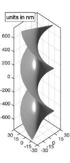
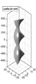
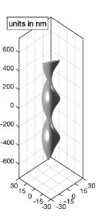
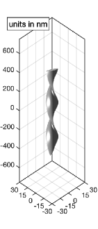
Figure 5.1: Optimized silver nanowires of length $L=2\lambda_{\mathrm{opt}}$ from Example 5.1 for $f_{\mathrm{opt}}=400,500,600,700$ THz (left to right).

In Figure 5.1 we show the optimized twisted silver nanowires obtained by the shape optimization for $L=2\lambda_{\mathrm{opt}}$ and $f_{\mathrm{opt}}=400,500,600$, and $700$ THz (left to right). The direction of the twist of the optimized structure depends on the initial guess. The aspect ratios $b/a$ of the elliptical cross-sections vary between $26.94$ at $f_{\mathrm{opt}}=400$ THz and $5.94$ at $f_{\mathrm{opt}}=700$ THz. The optimized twist rate per wave length of the cross-sections of the four optimized twisted silver nanowires around the straight spine curve is almost constant and virtually the same for all frequencies.

Silver
$f_{\mathrm{opt}}$ [THz]		$400$	$500$	$600$	$700$
$L=\frac{\lambda_{\mathrm{opt}}}{4}$	$J_{2}$	0.26	0.26	0.26	0.26
	$J_{\mathrm{HS}}$	0.12	0.12	0.12	0.12
$L=\frac{\lambda_{\mathrm{opt}}}{2}$	$J_{2}$	0.39	0.39	0.39	0.39
	$J_{\mathrm{HS}}$	0.17	0.17	0.17	0.17
$L=\lambda_{\mathrm{opt}}$	$J_{2}$	0.37	0.37	0.37	0.37
	$J_{\mathrm{HS}}$	0.20	0.20	0.20	0.20
$L=2\lambda_{\mathrm{opt}}$	$J_{2}$	0.32	0.32	0.32	0.32
	$J_{\mathrm{HS}}$	0.19	0.19	0.19	0.19

Gold
$f_{\mathrm{opt}}$ [THz]		$400$	$500$	$600$	$700$
$L=\frac{\lambda_{\mathrm{opt}}}{4}$	$J_{2}$	0.26	0.23	0.09	0.03
	$J_{\mathrm{HS}}$	0.12	0.12	0.02	0.003
$L=\frac{\lambda_{\mathrm{opt}}}{2}$	$J_{2}$	0.39	0.37	0.17	0.06
	$J_{\mathrm{HS}}$	0.17	0.17	0.03	0.004
$L=\lambda_{\mathrm{opt}}$	$J_{2}$	0.36	0.35	0.13	0.03
	$J_{\mathrm{HS}}$	0.20	0.19	0.04	0.003
$L=2\lambda_{\mathrm{opt}}$	$J_{2}$	0.32	0.30	0.08	0.01
	$J_{\mathrm{HS}}$	0.19	0.19	0.03	0.0008

Table 5.1: Normalized em-chirality measures $J_{2}$ and $J_{\mathrm{HS}}$ of optimized silver (left) and gold nanowires (right) from Example 5.1.

In Table 5.1 we collect the values of the normalized em-chirality measures $J_{2}$ and $J_{\mathrm{HS}}$ from (4.5) and (4.6) of the optimized straight twisted silver and gold nanowires for the four different frequencies and the four different length constraints. Each pair of entries in these tables corresponds to a different optimized twisted silver or gold nanowire. For the silver nanowires we observe that the values of $J_{2}$ and $J_{\mathrm{HS}}$ that are reached for the different optimized structures are independent of the frequency. On the other hand, for the optimized gold nanowires these values change significantly with frequency. While at $f_{\mathrm{opt}}=400$ and $500$ THz the normalized em-chirality measures of the optimized twisted gold nanowires are comparable to those of the optimized twisted silver nanowires, the normalized em-chirality measures of the optimized twisted gold nanowires quickly decrease at higher frequencies. This is a consequence of the increasing imaginary part of the relative electric permittivity of gold at higher frequencies (see Table 2.1). For the gold nanowires the aspect ratio $b/a$ of the elliptical cross-section varies between $20.11$ at $f_{\mathrm{opt}}=400$ THz and $1.69$ at $f_{\mathrm{opt}}=700$ THz, i.e., the cross-section is somewhat rounder than for the corresponding silver nanowires.

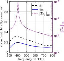
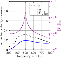
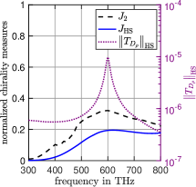
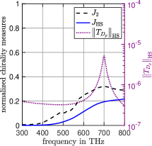
Figure 5.2: Frequency scans for optimized silver nanowires of length $L=2\lambda_{\mathrm{opt}}$ from Example 5.1 at $f_{\mathrm{opt}}=400,500,600,700$ THz (left to right).

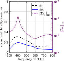
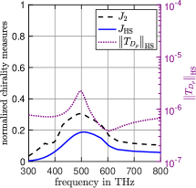
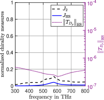
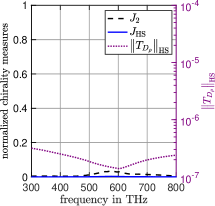
Figure 5.3: Frequency scans for optimized gold nanowires of length $L=2\lambda_{\mathrm{opt}}$ from Example 5.1 at $f_{\mathrm{opt}}=400,500,600,700$ THz (left to right).

Finally, we study the frequency dependence of the normalized em-chirality measures for the optimized twisted silver and gold nanowires of length $L=2\lambda_{\mathrm{opt}}$ that have been optimized at $f_{\mathrm{opt}}=400,500,600$, and $700$ THz. In each of the plots in Figure 5.2 and 5.3 the optimized nanowire is fixed. However, it is illuminated with incident waves of different frequencies, and thus its frequency-dependent relative electric permittivity $\varepsilon_{r}$ varies. In Figure 5.2 we plot the normalized em-chirality measures $J_{2}$ (dashed) and $J_{\mathrm{HS}}$ (solid) and an approximation of the total interaction cross-section (dotted) of the optimized thin twisted silver nanowires shown in Figure 5.1 over a frequency range between $300$ and $800$ THz. The approximation of the total interaction cross-section is obtained by evaluating the Hilbert-Schmidt norm of the operator $\mathcal{T}_{D_{\rho}}$ from (4.1) with $\rho=0.05/(k_{\mathrm{opt}}\sqrt{ab})$. The sharp peak in the total interaction cross-section is exactly at the plasmonic resonance frequency $f_{\mathrm{res}}$ of the corresponding thin silver nanowire. It is important to note that, in contrast to the normalized em-chirality measures, the total interaction cross-section is plotted in a logarithmic scale. We find that $J_{2}$ and $J_{\mathrm{HS}}$ have a peak at the plasmonic resonance frequency $f_{\mathrm{res}}$ as well. This is the frequency that has been used in the shape optimization, i.e., $f_{\mathrm{opt}}=f_{\mathrm{res}}$.

In Figure 5.3 we show the corresponding frequency scans for the optimized thin twisted gold nanowires. For the gold nanowires that have been optimized at $f_{\mathrm{opt}}=400$ and $500$ THz, the results are similar as for the silver nanowires that have been optimized at the same frequencies in Figure 5.2. On the other hand, for the gold nanowires optimized at $f_{\mathrm{opt}}=600$ and $700$ THz, the plasmonic resonance is no longer visible in the plots of the total interaction cross-section. This is a consequence of the larger imaginary part of the electric permittivity of gold at $f_{\mathrm{opt}}=600,700$ THz (see Table 2.1). For these two higher frequencies, the values of the normalized em-chirality measures $J_{2}$ and $J_{\mathrm{HS}}$ are small across the entire frequency band. The plasmonic resonance seems to be required to obtain thin metallic nanowires that exhibit large normalized em-chirality measures.  $\lozenge$

Example 5.2 (Optimizing the shape of the spine curve of the nanowire).

In our second example we consider a free-form shape optimization for the spine curve of thin silver and gold nanowires with elliptical cross sections, but we do not optimize the twist rate of the cross-section of the nanowire along the spine curve. As in the first example, we consider four different frequencies $f_{\mathrm{opt}}=400,500,600$, and $700$ THz, and for each of these frequencies we again choose the aspect ratio of the elliptical cross-section of the nanowire such that $f_{\mathrm{opt}}=f_{\mathrm{res}}$ is a plasmonic resonance frequency for the nanowire. We use the optimization scheme from Section 4. For the regularization parameters in (4.16) we choose $\alpha_{1}=5$, $\alpha_{2}=8\times 10^{-3}$, and $\alpha_{3}=0$.

The length constraint for the nanowire is set to be $L=3\lambda_{\mathrm{opt}}/2$, and, accordingly, we choose the maximal degree $N$ of circularly polarized vector spherical harmonics that is used in the discretization of the operator ${\bm{T}}_{\rho}({\bm{p}},V_{{\bm{p}},\theta})$ and of its Fréchet derivative ${\bm{T}}_{\rho}^{\prime}[{\bm{p}},V_{{\bm{p}},\theta}]({\bm{h}},\phi)$ (see Remark 4.4) to be $N=5$. We use cubic not-a-knot splines with $n=20$ knots to parametrize the spine curve $\Gamma$ and the (fixed) twist function $\theta$ and $11$ quadrature points on each spline segment to discretize line integrals over $\Gamma$. For the initial guess for the spine curve we use a straight line of length $L=3\lambda_{\mathrm{opt}}/2$, and we add a small random perturbation to obtain an em-chiral configuration. The same random perturbation is used for all frequencies. The initial geometry adapted frame is chosen to be rotation minimizing.

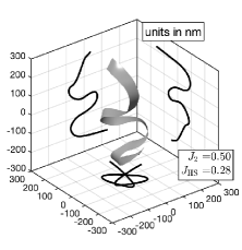
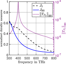
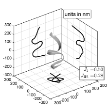
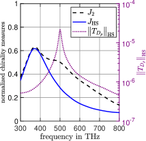
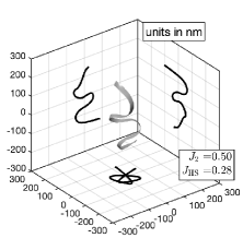
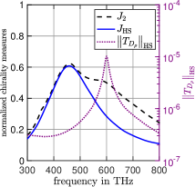
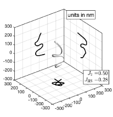
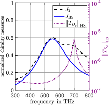
Figure 5.4: Optimized silver nanowires and corresponding frequency scans from Example 5.2 for $f_{\mathrm{opt}}=400,500$ THz (top row) and $f_{\mathrm{opt}}=600,700$ THz (bottom row).

In Figure 5.4 we show the optimized silver nanowires that have been obtained by the shape optimization for $f_{\mathrm{opt}}=400,500,600$, and $700$ THz. The aspect ratios $b/a$ of the elliptical cross-sections are the same as in Example 5.1 and vary between $26.94$ at $f_{\mathrm{opt}}=400$ THz and $5.94$ at $f_{\mathrm{opt}}=700$ THz. For a better three-dimensional impression, we also included the projections of the spine curves of the optimized nanowires on the three coordinate planes in these plots. During the optimization the straight initial guess bends into a rather irregular shape that is difficult to interpret. However the optimized silver nanowires obtained at the four different frequencies have very similar shapes, which seem to be rescaled versions of each other with respect to the wave length.

Figure 5.4 also contains plots illustrating the frequency dependence of the normalized em-chirality measures $J_{2}$ (dashed) and $J_{\mathrm{HS}}$ (solid) as well as of the total interaction cross-section (dotted) of the optimized silver nanowires. The maxima of the normalized em-chirality measures and the plasmonic resonances visible in the plots of the total interaction cross-section are rather localized. It is interesting to observe that, although the shape optimization has been carried out at the plasmonic resonance frequency, i.e., $f_{\mathrm{opt}}=f_{\mathrm{res}}$, the maximum of the normalized em-chirality measures $J_{2}$ and $J_{\mathrm{HS}}$ is attained around $100$ to $150$ THz below the plasmonic resonance frequency in all four examples. This is a common feature that we have observed in several other examples, and we will utilize this phenomenon in Example 5.3 below to design thin silver and gold nanowires with even higher em-chirality measures.

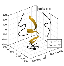
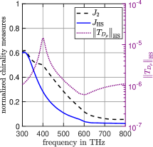
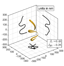
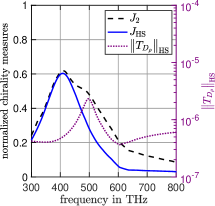
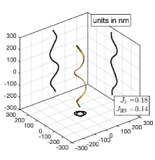
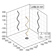
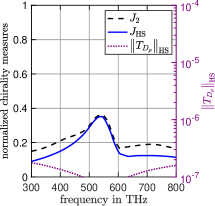
Figure 5.5: Optimized gold nanowires and corresponding frequency scans from Example 5.2 for $f_{\mathrm{opt}}=400,500$ THz (top row) and $f_{\mathrm{opt}}=600,700$ THz (bottom row).

In Figure 5.5 we show the corresponding results of the shape optimization of thin gold nanowires for $f_{\mathrm{opt}}=400,500,600$, and $700$ THz. The shapes of the gold nanowires that have been optimized at $f_{\mathrm{opt}}=400,500$ THz are similar to those of the optimized thin silver nanowires in Figure 5.4. Also the frequency scans in Figure 5.5 show a similar behavior, although the plasmonic resonance is not as pronounced as for the silver nanowires. For $f_{\mathrm{opt}}=600,700$ THz the results are different. The shapes of the optimized gold nanowires look similar to those obtained for dielectric nanowires in [6]. The optimized gold nanowires are helices, and no plasmonic resonances are visible in the plots of the total interaction cross-sections. This different behavior results from the larger imaginary part of the electric permittivity of gold at $f_{\mathrm{opt}}=600,700$ THz (see Table 2.1).  $\lozenge$

Example 5.3 (Optimizing the twist rate of the cross-section and the shape of the spine curve of the nanowire).

The goal of our final example is to design thin silver and gold nanowires with elliptical cross-sections that possess normalized em-chirality measures $J_{2}$ and $J_{\mathrm{HS}}$ as close to $1$ as possible at optical frequencies. We consider a free-form shape optimization for the spine curve of the nanowire, and we optimize the twisting of the elliptical cross-section of the nanowire along the spine curve. As in the previous examples, we discuss four different frequencies $f_{\mathrm{opt}}=400,500,600$, and $700$ THz. For each of these frequencies we choose the aspect ratio of the elliptical cross-section of the nanowire such that its plasmonic resonance frequency $f_{\mathrm{res}}$ is around $100$ to $150$ Thz above the frequency $f_{\mathrm{opt}}$ that is used in the shape optimization, i.e., we use $b/a=12.5$ at $f_{\mathrm{opt}}=400$ THz, $b/a=7.14$ at $f_{\mathrm{opt}}=500$ THz, $b/a=3.85$ at $f_{\mathrm{opt}}=600$ THz, and $b/a=1.92$ at $f_{\mathrm{opt}}=700$ THz. In particular $f_{\mathrm{opt}}\not=f_{\mathrm{res}}$. This is different from the previous two examples, where we optimized the shape of the nanowires directly at the plasmonic resonance frequency. It is motivated by our observations at the end of Example 5.2. We apply the optimization scheme from Section 4. For the regularization parameters in (4.16) we choose $\alpha_{1}=5$, $\alpha_{2}=8\times 10^{-3}$ and $\alpha_{3}=1\times 10^{-6}$.

The outcome of the shape optimization strongly depends on the initial guess for the spine curve. Thus, we consider in this example $100$ different initial spine curves for the optimization scheme at each frequency. These are helices with four turns, where the total height and the radius of the helix are chosen randomly in $[0,2\lambda_{\mathrm{opt}}/3]$ and in $[0,\lambda_{\mathrm{opt}}/2]$, respectively. As before, $\lambda_{\mathrm{opt}}$ denotes the wave length at the frequency $f_{\mathrm{opt}}$. We also add different random twists to these initial guesses. We use cubic not-a-knot splines with $n=40$ knots to parametrize the spine curve and the twist function, and $21$ quadrature points on each spline segment to discretize line integrals over $\Gamma$. We choose the maximal degree $N$ of circularly polarized vector spherical harmonics that is used in the discretization of the operator ${\bm{T}}_{\rho}({\bm{p}},V_{{\bm{p}},\theta})$ and of its Fréchet derivative ${\bm{T}}_{\rho}^{\prime}[{\bm{p}},V_{{\bm{p}},\theta}]({\bm{h}},\phi)$ (see Remark 4.4) to be $N=5$. This gives $100$ different optimized silver and gold nanowires for each frequency $f_{\mathrm{opt}}$, and we finally select those (for each frequency $f_{\mathrm{opt}}$) that attain the highest normalized em-chirality measures.

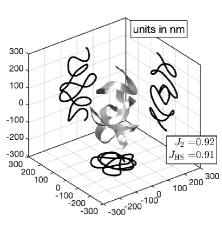
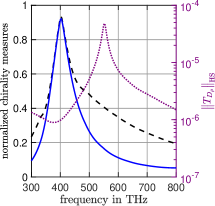
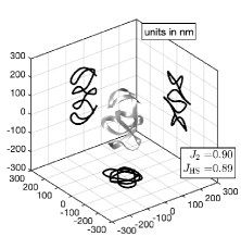
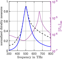
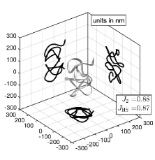
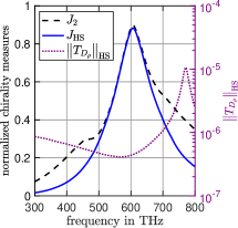
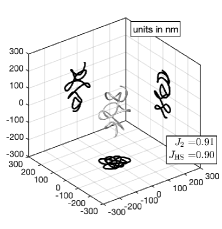
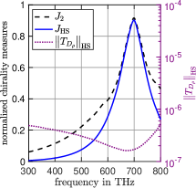
Figure 5.6: Optimized silver nanowires and corresponding frequency scans from Example 5.3 for $f_{\mathrm{opt}}=400,500$ THz (top row) and for $f_{\mathrm{opt}}=600,700$ THz (bottom row).

In Figure 5.6 we show the optimized silver nanowires that have been obtained for $f_{\mathrm{opt}}=400,500$ THz (top row) and for $f_{\mathrm{opt}}=600,700$ THz (bottom row). The shapes of the optimized nanowires look complicated but they show similarities and seem to be scaled according to the wavelength, where the optimization has been carried out. Very high normalized em-chirality measures are being attained by the optimized structures at all four frequencies $f_{\mathrm{opt}}=400,500,600$, and $700$ THz, respectively. Figure 5.6 also shows plots of the normalized em-chirality measures $J_{2}$ (dashed) and $J_{\mathrm{HS}}$ (solid) as well as of the total interaction cross-section (dotted) of the optimized thin silver nanowires as a function of the frequency of the incident waves. The maximal values of the normalized em-chirality measures appear at approximately the same frequency, where the total interaction cross-section of the nanowires has a local minimum. Directly at the plasmonic resonance frequency the normalized em-chirality measures are smaller, but on the other hand the total interaction cross section of the nanowire is much larger.

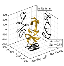
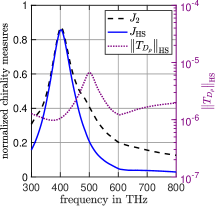
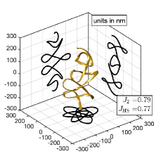
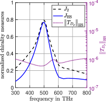
Figure 5.7: Optimized gold nanowires and corresponding frequency scans from Example 5.3 for $f_{\mathrm{opt}}=400,500$ THz.

In Figure 5.7 we show the corresponding results for gold nanowires at $f_{\mathrm{opt}}=400$ and $500$ THz. The obtained normalized em-chirality measures are lower than for silver, which might be explained by the larger imaginary part of the relative electric permittivity of gold at these frequencies. Also the plasmonic resonances are not as pronounced as for the thin silver nanowires. As a consequence of the even larger imaginary part of the electric permittivity of gold at $f_{\mathrm{opt}}=600$ and $700$ THz, the normalized em-chirality measures obtained for thin gold nanowires optimized at these frequencies are rather small. Therefore, we do not show the results for these frequencies.  $\lozenge$

Conclusions

We have optimized the shape of thin free-form silver and gold nanowires to maximize their electromagnetic chirality at particular frequencies in the optical band. Our gradient based shape optimization scheme uses an asymptotic representation formula for scattered electromagnetic fields due to thin bended and twisted metallic nanowires with arbitrary cross-sections to efficiently evaluate the objective functionals and their shape derivatives in each iteration. We have extended the theoretical foundation of this asymptotic representation formula from dielectric materials to noble metals with complex-valued electric permittivities with negative real and positive imaginary parts.

We have demonstrated that the optimized free-form silver and gold nanowires yield significantly enhanced chiral responses, when compared to traditional helical designs. Values larger than $90$% of the maximum possible value of electromagnetic chirality are obtained for optimized silver nanowires with elliptical cross-section across the whole optical band. We have observed an interesting connection between plasmonic resonances (and nearby local minima of the total interaction cross-section) and extremal values of electromagnetic chirality for thin metallic nanowires at optical frequencies. These results are relevant in practice, since the optimized free-form silver and gold nanowires may serve as building blocks of novel metamaterials with an increased chiral response. However, due to the small thickness of our optimized nanowires, the fabrication of these metamaterials might be challenging.

Appendix A Polarization tensor bounds

We show two pointwise bounds for the electric polarization tensor $\mathbb{M}^{\varepsilon}$ that are similar to the bounds that have been established in [12, Thm. 1] but valid for complex valued relative electric permittivities $\varepsilon_{r}$ with negative real and positive imaginary part. Since we will modify the arguments used in the proof of [12, Thm. 1], we work with the following definition of the electric polarization tensor $\mathbb{M}^{\varepsilon}$, which is equivalent to (2.12)–(2.13) (see [13, Lmm. 1]). For any $\bm{\xi}\in{S^{2}}$, we denote by $V_{\rho}^{(\bm{\xi})}\in H^{1}_{\diamond}({B_{R}(0)})$ the corrector potential satisfying

$$\mathrm{div}\bigl{(}\varepsilon_{\rho}\nabla V_{\rho}^{(\bm{\xi})}\bigr{)}\,=\,0\quad\text{in }{B_{R}(0)}\,,\qquad\varepsilon_{\rho}\frac{\partial V_{\rho}^{(\bm{\xi})}}{\partial{\bm{\nu}}}\,=\,\varepsilon_{\rho}\,{\bm{\nu}}\cdot\bm{\xi}\quad\text{on }\partial{B_{R}(0)}\,,$$ (A.1)

where $H^{1}_{\diamond}({B_{R}(0)})$ denotes the space of $H^{1}$-functions on ${B_{R}(0)}$ with vanishing integral mean on $\partial{B_{R}(0)}$. Then, the electric polarization tensor $\mathbb{M}^{\varepsilon}\in L^{2}(\Gamma,{{\mathbb{C}}^{3\times 3}})$ is uniquely determined by

$$\frac{1}{|\Gamma|}\int_{\Gamma}\bm{\xi}\cdot\mathbb{M}^{\varepsilon}\bm{\xi}\,\psi\,\operatorname{d\!}s\,=\,\frac{1}{|D_{\rho}|}\int_{D_{\rho}}\bigl{(}\bm{\xi}\cdot\nabla V^{(\bm{\xi})}_{\rho}\bigr{)}\,\psi\,\operatorname{d\!}{\bm{x}}+o(1)\qquad\text{as }\rho\to 0$$ (A.2)

for all $\psi\in C(\overline{{B_{R}(0)})})$ and any $\bm{\xi}\in{S^{2}}$.

Lemma A.1.

Suppose that $\varepsilon_{r}\in{\mathbb{C}}$ with $\operatorname{Re}(\varepsilon_{r})<0$ and $\operatorname{Im}(\varepsilon_{r})>0$, and for any $0<\rho<r$ let $D_{\rho}\subseteq{{\mathbb{R}}^{3}}$ and $\varepsilon_{\rho}$ be as in (2.4) and (2.9), respectively. As before, we write $\varepsilon_{m}:=\varepsilon_{0}\varepsilon_{r}$ for the electric permittivity of the thin metallic nanowire.

• The electric polarization tensor $\mathbb{M}^{\varepsilon}\in L^{2}(\Gamma,{{\mathbb{C}}^{3\times 3}})$ is symmetric, i.e.,

  $$\mathbb{M}^{\varepsilon}_{ij}({\bm{x}})\,=\,\mathbb{M}^{\varepsilon}_{ji}({\bm{x}})\qquad\text{for }1\leq i,j\leq 3\text{ and a.e.\ }{\bm{x}}\in\Gamma\,.$$ (A.3)

• We have that

  $$\frac{\bm{\xi}\cdot\operatorname{Im}\bigl{(}(\overline{\varepsilon_{m}-\varepsilon_{0}})\mathbb{M}^{\varepsilon}({\bm{x}})\bigr{)}\bm{\xi}}{\operatorname{Im}\left(\overline{\varepsilon_{m}-\varepsilon_{0}}\right)}\,\leq\,|\bm{\xi}|^{2}\qquad\text{for every }\bm{\xi}\in{S^{2}}\text{ and a.e.\ }{\bm{x}}\in\Gamma\,.$$ (A.4)

• There exists $\gamma\in(0,\pi/2)$ such that $\operatorname{Re}(\mathrm{e}^{\mathrm{i}\gamma}\overline{\varepsilon_{0}})>0$, $\operatorname{Re}(\mathrm{e}^{\mathrm{i}\gamma}\overline{\varepsilon_{m}})>0$, and $\operatorname{Re}(\mathrm{e}^{\mathrm{i}\gamma}(\overline{\varepsilon_{m}-\varepsilon_{0}}))<0$. For every $\gamma$ with these properties, we have that

  $$\frac{\bm{\xi}\cdot\operatorname{Re}\bigl{(}\mathrm{e}^{\mathrm{i}\gamma}(\overline{\varepsilon_{m}-\varepsilon_{0}})\mathbb{M}^{\varepsilon}({\bm{x}})\bigr{)}\bm{\xi}}{\operatorname{Re}\left(\mathrm{e}^{\mathrm{i}\gamma}(\overline{\varepsilon_{m}-\varepsilon_{0}})\right)}\,\geq\,|\bm{\xi}|^{2}\qquad\text{for every }\bm{\xi}\in{S^{2}}\text{ and a.e.\ }{\bm{x}}\in\Gamma\,.$$ (A.5)

Proof.

(a)  Let $\bm{\xi}\in{S^{2}}$. We denote by $V_{\rho}^{(\bm{\xi})}\in H^{1}_{\diamond}({B_{R}(0)})$ the corresponding solution to (A.1). Moreover, we define $V_{0}^{(\bm{\xi})}\in H^{1}_{\diamond}({B_{R}(0)})$ by $V_{0}^{(\bm{\xi})}({\bm{x}}):={\bm{x}}\cdot\bm{\xi}$ for all ${\bm{x}}\in{B_{R}(0)}$. Then, $V_{0}^{(\bm{\xi})}$ solves (A.1) with $\varepsilon_{\rho}$ replaced by $\varepsilon_{0}$.

It can be seen as on p. 169 of [12] that, for any two $\bm{\xi},{\bm{\eta}}\in{S^{2}}$ and for all $\psi\in C(\overline{{B_{R}(0)}})$,

$$\frac{1}{|D_{\rho}|}\int_{D_{\rho}}(\varepsilon_{0}-\varepsilon_{m})\nabla V_{0}^{(\bm{\xi})}\cdot\nabla V_{\rho}^{({\bm{\eta}})}\,\psi\,\operatorname{d\!}{\bm{x}}\,=\,\frac{1}{|D_{\rho}|}\int_{D_{\rho}}(\varepsilon_{0}-\varepsilon_{m})\nabla V_{0}^{({\bm{\eta}})}\cdot\nabla V_{\rho}^{(\bm{\xi})}\,\psi\,\operatorname{d\!}{\bm{x}}+o(1)$$

as $\rho\to 0$. Substituting this into (A.2) gives

$$\frac{1}{|\Gamma|}\int_{\Gamma}(\varepsilon_{0}-\varepsilon_{m})\bm{\xi}\cdot\mathbb{M}^{\varepsilon}{\bm{\eta}}\,\psi\,\operatorname{d\!}s\,=\,\frac{1}{|\Gamma|}\int_{\Gamma}(\varepsilon_{0}-\varepsilon_{m}){\bm{\eta}}\cdot\mathbb{M}^{\varepsilon}\bm{\xi}\,\psi\,\operatorname{d\!}s+o(1)\,,$$

which implies (A.3).

(b)  The same calculation as on p. 170 of [12] shows that, for any $\bm{\xi}\in{S^{2}}$,

$$\frac{1}{|\Gamma|}\int_{\Gamma}(\overline{\varepsilon_{m}-\varepsilon_{0}})\bm{\xi}\cdot\mathbb{M}^{\varepsilon}\bm{\xi}\,\psi\,\operatorname{d\!}s\,=\,\frac{1}{|D_{\rho}|}\int_{D_{\rho}}(\overline{\varepsilon_{m}-\varepsilon_{0}})\nabla V_{\rho}^{(\bm{\xi})}\cdot\nabla V_{0}^{(\bm{\xi})}\,\psi\,\operatorname{d\!}{\bm{x}}\\ \,=\,\frac{1}{|D_{\rho}|}\int_{D_{\rho}}(\overline{\varepsilon_{m}-\varepsilon_{0}})|\nabla V_{0}^{(\bm{\xi})}|^{2}\,\psi\,\operatorname{d\!}{\bm{x}}-\frac{1}{|D_{\rho}|}\int_{B_{R}(0)}\overline{\varepsilon_{\rho}}|\nabla(V^{(\bm{\xi})}_{0}-V^{(\bm{\xi})}_{\rho})|^{2}\,\psi\,\operatorname{d\!}{\bm{x}}+o(1)$$ (A.6)

as $\rho\to 0$. From now on we consider non-negative test functions $\psi\in C(\overline{{B_{R}(0)}})$, i.e., $\psi\geq 0$. Taking the imaginary part on both sides of (A.6) and recalling that $\operatorname{Im}(\varepsilon_{\rho})\geq 0$ gives

$$\frac{1}{|\Gamma|}\int_{\Gamma}\bm{\xi}\cdot\operatorname{Im}\bigl{(}(\overline{\varepsilon_{m}-\varepsilon_{0}})\mathbb{M}^{\varepsilon}\bigr{)}\bm{\xi}\,\psi\,\operatorname{d\!}s\,\geq\,\frac{1}{|D_{\rho}|}\int_{D_{\rho}}\operatorname{Im}\bigl{(}\overline{\varepsilon_{m}-\varepsilon_{0}}\bigr{)}|\nabla V_{0}^{(\bm{\xi})}|^{2}\,\psi\,\operatorname{d\!}{\bm{x}}+o(1)$$ (A.7)

as $\rho\to 0$. Passing to the limit on the right hand side of (A.7) then yields (A.4).

(c)  Writing $\overline{\varepsilon_{m}}=|\varepsilon_{m}|\mathrm{e}^{\mathrm{i}\alpha}$ and $\overline{\varepsilon_{m}-\varepsilon_{0}}=|\varepsilon_{m}-\varepsilon_{0}|\mathrm{e}^{\mathrm{i}\beta}$ in polar form, our assumptions on $\varepsilon_{0}$ and $\varepsilon_{m}$ imply that $\alpha,\beta\in(\pi,3\pi/2)$ with $\alpha>\beta$. Accordingly, choosing $\gamma=3\pi/2-(\alpha+\beta)/2$, we obtain that $\gamma\in(0,\pi/2)$ with $\operatorname{Re}(\mathrm{e}^{\mathrm{i}\gamma}\overline{\varepsilon_{0}})>0$, $\operatorname{Re}(\mathrm{e}^{\mathrm{i}\gamma}\overline{\varepsilon_{m}})>0$, and $\operatorname{Re}(\mathrm{e}^{\mathrm{i}\gamma}(\overline{\varepsilon_{m}-\varepsilon_{0}}))<0$. Multiplying both sides of (A.6) with $\mathrm{e}^{\mathrm{i}\gamma}$ and taking the real part gives

$$\frac{1}{|\Gamma|}\int_{\Gamma}\bm{\xi}\cdot\operatorname{Re}\bigl{(}\mathrm{e}^{\mathrm{i}\gamma}(\overline{\varepsilon_{m}-\varepsilon_{0}})\mathbb{M}^{\varepsilon}\bigr{)}\bm{\xi}\,\psi\,\operatorname{d\!}s\,\leq\,\frac{1}{|D_{\rho}|}\int_{D_{\rho}}\operatorname{Re}\bigl{(}\mathrm{e}^{\mathrm{i}\gamma}(\overline{\varepsilon_{m}-\varepsilon_{0}})\bigr{)}|\nabla V_{0}^{(\bm{\xi})}|^{2}\,\psi\,\operatorname{d\!}{\bm{x}}+o(1)$$ (A.8)

as $\rho\to 0$. Passing to the limit on the right hand side of (A.8) then yields (A.5). ∎

References

- [1] G. S. Alberti and Y. Capdeboscq. Lectures on elliptic methods for hybrid inverse problems, volume 25 of Cours Spécialisés. Société Mathématique de France, Paris, 2018.
- [2] H. Ammari, Y. T. Chow, K. Liu, and J. Zou. Optimal shape design by partial spectral data. SIAM J. Sci. Comput., 37(6):B855–B883, 2015.
- [3] H. Ammari, Y. Deng, and P. Millien. Surface plasmon resonance of nanoparticles and applications in imaging. Arch. Ration. Mech. Anal., 220(1):109–153, 2016.
- [4] H. Ammari, K. Hamdache, and J.-C. Nédélec. Chirality in the Maxwell equations by the dipole approximation. SIAM J. Appl. Math., 59(6):2045–2059, 1999.
- [5] H. Ammari and H. Kang. Polarization and moment tensors, volume 162 of Applied Mathematical Sciences. Springer, New York, 2007.
- [6] T. Arens, R. Griesmaier, and M. Knöller. Maximizing the electromagnetic chirality of thin dielectric tubes. SIAM J. Appl. Math., 81(5):1979–2006, 2021.
- [7] T. Arens, F. Hagemann, F. Hettlich, and A. Kirsch. The definition and measurement of electromagnetic chirality. Math. Methods Appl. Sci., 41(2):559–572, 2018.
- [8] E. Beretta, Y. Capdeboscq, F. de Gournay, and E. Francini. Thin cylindrical conductivity inclusions in a three-dimensional domain: a polarization tensor and unique determination from boundary data. Inverse Problems, 25(6):065004, 22, 2009.
- [9] R. L. Bishop. There is more than one way to frame a curve. Amer. Math. Monthly, 82:246–251, 1975.
- [10] M. Brühl, M. Hanke, and M. S. Vogelius. A direct impedance tomography algorithm for locating small inhomogeneities. Numer. Math., 93(4):635–654, 2003.
- [11] Y. Capdeboscq, R. Griesmaier, and M. Knöller. An asymptotic representation formula for scattering by thin tubular structures and an application in inverse scattering. Multiscale Model. Simul., 19(2):846–885, 2021.
- [12] Y. Capdeboscq and M. S. Vogelius. A general representation formula for boundary voltage perturbations caused by internal conductivity inhomogeneities of low volume fraction. M2AN Math. Model. Numer. Anal., 37(1):159–173, 2003.
- [13] Y. Capdeboscq and M. S. Vogelius. Pointwise polarization tensor bounds, and applications to voltage perturbations caused by thin inhomogeneities. Asymptot. Anal., 50(3-4):175–204, 2006.
- [14] D. Colton and R. Kress. Inverse acoustic and electromagnetic scattering theory, volume 93 of Applied Mathematical Sciences. Springer, Cham, fourth edition, 2019.
- [15] K. Eppler and H. Harbrecht. Fast wavelet BEM for 3d electromagnetic shaping. Appl. Numer. Math., 54(3):537–554, 2005.
- [16] I. Fernandez-Corbaton, M. Fruhnert, and C. Rockstuhl. Objects of maximum electromagnetic chirality. Phys. Rev. X, 6(3):031013, 2016.
- [17] I. Fernandez-Corbaton, C. Rockstuhl, P. Ziemke, P. Gumbsch, A. Albiez, R. Schwaiger, T. Frenzel, M. Kadic, and M. Wegener. New twists of 3d chiral metamaterials. Adv. Mater., 31(26):1807742, 2019.
- [18] J. K. Gansel, M. Latzel, A. Frölich, J. Kaschke, M. Thiel, and M. Wegener. Tapered gold-helix metamaterials as improved circular polarizers. Appl. Phys. Lett., 100(10):101109, 2012.
- [19] J. K. Gansel, M. Thiel, M. S. Rill, M. Decker, K. Bade, V. Saile, G. von Freymann, S. Linden, and M. Wegener. Gold helix photonic metamaterial as broadband circular polarizer. Science, 325(5947):1513–1515, 2009.
- [20] J. K. Gansel, M. Wegener, S. Burger, and S. Linden. Gold helix photonic metamaterials: a numerical parameter study. Opt. Express, 18(2):1059–1069, 2010.
- [21] X. Garcia-Santiago, M. Hammerschmidt, J. Sachs, S. Burger, H. Kwon, M. Knöller, T. Arens, P. Fischer, I. Fernandez-Corbaton, and C. Rockstuhl. Toward maximally electromagnetically chiral scatterers at optical frequencies. ACS Photonics, 9(6):1954–1964, 2022.
- [22] J.-J. Greffet. Introduction to surface plasmon theory. In S. Enoch and N. Bonod, editors, Plasmonics: From Basics to Advanced Topics, pages 105–148. Springer Berlin Heidelberg, Berlin, Heidelberg, 2012.
- [23] D. Grieser. The plasmonic eigenvalue problem. Rev. Math. Phys., 26(3):1450005, 26, 2014.
- [24] R. Griesmaier. Reconstruction of thin tubular inclusions in three-dimensional domains using electrical impedance tomography. SIAM J. Imaging Sci., 3(3):340–362, 2010.
- [25] R. Griesmaier. A general perturbation formula for electromagnetic fields in presence of low volume scatterers. ESAIM Math. Model. Numer. Anal., 45(6):1193–1218, 2011.
- [26] R. Griesmaier and N. Hyvönen. A regularized Newton method for locating thin tubular conductivity inhomogeneities. Inverse Problems, 27(11):115008, 22, 2011.
- [27] R. Griesmaier and J. Sylvester. Uncertainty principles for inverse source problems for electromagnetic and elastic waves. Inverse Problems, 34(6):065003, 37, 2018.
- [28] H. Haddar, Z. Jiang, and M. K. Riahi. A robust inversion method for quantitative 3D shape reconstruction from coaxial eddy current measurements. J. Sci. Comput., 70(1):29–59, 2017.
- [29] F. Hagemann. Reconstructing the shape and measuring chirality of obstacles in electromagnetic scattering. PhD thesis, Karlsruhe Institute of Technology (KIT), 2019.
- [30] F. Hagemann, T. Arens, T. Betcke, and F. Hettlich. Solving inverse electromagnetic scattering problems via domain derivatives. Inverse Problems, 35(8):084005, 20, 2019.
- [31] F. Hagemann and F. Hettlich. Application of the second domain derivative in inverse electromagnetic scattering. Inverse Problems, 36(12):125002, 34, 2020.
- [32] M. Hentschel, M. Schäferling, X. Duan, H. Giessen, and N. Liu. Chiral plasmonics. Sci. Adv., 3(5):e1602735, 2017.
- [33] M. Hintermüller, A. Laurain, and I. Yousept. Shape sensitivities for an inverse problem in magnetic induction tomography based on the eddy current model. Inverse Problems, 31(6):065006, 25, 2015.
- [34] K. Höflich, T. Feichtner, E. Hansjürgen, C. Haverkamp, H. Kollmann, C. Lienau, and M. Silies. Resonant behavior of a single plasmonic helix. Optica, 6(9):1098–1105, Sep 2019.
- [35] P. B. Johnson and R. W. Christy. Optical constants of the noble metals. Phys. Rev. B, 6:4370–4379, Dec 1972.
- [36] M. Kadic, G. W. Milton, M. van Hecke, and M. Wegener. 3d metamaterials. Nat. Rev. Phys., 1(3):198–210, 2019.
- [37] J. Kaschke and M. Wegener. Gold triple-helix mid-infrared metamaterial by sted-inspired laser lithography. Opt. Lett., 40(17):3986–3989, 2015.
- [38] N. Lebbe, C. Dapogny, E. Oudet, K. Hassan, and A. Gliere. Robust shape and topology optimization of nanophotonic devices using the level set method. J. Comput. Phys., 395:710–746, 2019.
- [39] D.-H. Li and M. Fukushima. On the global convergence of the BFGS method for nonconvex unconstrained optimization problems. SIAM J. Optim., 11(4):1054–1064, 2001.
- [40] P. Monk. Finite element methods for Maxwell’s equations. Numerical Mathematics and Scientific Computation. Oxford University Press, New York, 2003.
- [41] L. Novotny and B. Hecht. Principles of Nano-Optics. Cambridge University Press, Cambridge, second edition, 2012.
- [42] J. Semmler, L. Pflug, M. Stingl, and G. Leugering. Shape optimization in electromagnetic applications. In A. Pratelli and G. Leugering, editors, New Trends in Shape Optimization, pages 251–269. Springer, Cham, 2015.
- [43] W. Śmigaj, T. Betcke, S. Arridge, J. Phillips, and M. Schweiger. Solving boundary integral problems with BEM++. ACM Trans. Math. Software, 41(2):Art. 6, 40, 2015.
- [44] V. K. Valev, J. J. Baumberg, C. Sibilia, and T. Verbiest. Chirality and chiroptical effects in plasmonic nanostructures: Fundamentals, recent progress, and outlook. Adv. Mater., 25(18):2517–2534, 2013.
- [45] M. Vavilin and I. Fernandez-Corbaton. Multidimensional measures of electromagnetic chirality and their conformal invariance. New J. Phys., 24(3):033022, 2022.
- [46] W. Wang, B. Jüttler, D. Zheng, and Y. Liu. Computation of rotation minimizing frames. ACM Trans. Graph., 27(1):1–18, 2008.