Velocity estimation via model order reduction

Abstract

A novel approach to full waveform inversion (FWI), based on a data driven reduced order model (ROM) of the wave equation operator is introduced. The unknown medium is probed with pulses and the time domain pressure waveform data is recorded on an active array of sensors. The ROM, a projection of the wave equation operator is constructed from the data via a nonlinear process and is used for efficient velocity estimation. While the conventional FWI via nonlinear least-squares data fitting is challenging without low frequency information, and prone to getting stuck in local minima (cycle skipping), minimization of ROM misfit is behaved much better, even for a poor initial guess. For low-dimensional parametrizations of the unknown velocity the ROM misfit function is close to convex. The proposed approach consistently outperforms conventional FWI in standard synthetic tests.

1 Introduction

We consider the inverse problem of velocity estimation from time-domain reflection data recorded by an array of $m$ sensors that can both emit and record. For simplicity we work with the acoustic wave equation with unknown velocity $c({{\itbf x}})$. The proposed approach can be extended to vectorial (elastic) waves.

The model pressure wave $p^{(s)}(t,{{\itbf x}})$ generated by the $s^{\rm th}$ sensor, for $s=1,\ldots,m$, satisfies the initial value problem

$$\big{[}\partial_{t}^{2}-c^{2}({{\itbf x}})\Delta\big{]}p^{(s)}(t,{{\itbf x}}) =f^{\prime}(t)\theta({{\itbf x}}-{{\itbf x}}_{s}),\quad t\in\mathbb{R},$$ (1)

$$p^{(s)}(t,{{\itbf x}}) =0,\quad t<-t_{f},$$ (2)

for ${{\itbf x}}\in\Omega$, a simply connected domain in two or three dimensions, with boundary $\partial\Omega$. We set homogeneous boundary conditions (Dirichlet, Neumann, or a combination thereof) on $\partial\Omega$. We assume the sensors in the array to be identical, modeled by a function $\theta({{\itbf x}})$, with small support around the origin. Each sensor emits the probing pulse $f(t)$, supported on $(-t_{f},t_{f})$. For simplicity we take $f(t)$ to be an even function, with a non-negative Fourier transform $\widehat{f}(\omega)\geq 0$ that is analytic.

The inverse problem is to estimate the velocity $c({{\itbf x}})$ from the measurements

$$\mathcal{M}^{(r,s)}(t)=\int_{\Omega}d{{\itbf x}}\,\theta({{\itbf x}}-{{\itbf x}}_{r})p^{(s)}(t,{{\itbf x}}),$$ (3)

for $s,r=1,\ldots,m$ and $t\in[0,T]$. Conventional FWI approach to velocity estimation, see, e.g., Tarantola, (1984), suffers from a fundamental flaw: the objective function is nonconvex with numerous local minima. This effect makes any local optimization algorithm unlikely to succeed, in the absence of an accurate starting guess, see Santosa and Symes, (1989). We address this issue by reformulating the optimization problem for velocity estimation using ROM.

2 Theory

2.1 Symmetrized wave operator and data model

It is convenient to work with a self-adjoint wave operator

$${\cal A}=-c({{\itbf x}})\Delta\big{[}c({{\itbf x}})\cdot\big{]},$$ (4)

a similarity transformation of $-c^{2}({{\itbf x}})\Delta$, the wave operator of equation 1. To obtain the ROM of ${\cal A}$, we introduce the even in time wave

$${\rm w}^{(s)}(t,{{\itbf x}})=\frac{\big{[}p^{(s)}(t,{{\itbf x}})+p^{(s)}(-t,{{\itbf x}})]}{c({{\itbf x}})},$$ (5)

and “the data”, an $m\times m$ matrix ${\itbf D}(t)$, with entries

$$D^{(r,s)}(t)=\frac{\mathcal{M}^{(r,s)}(t)+\mathcal{M}^{(r,s)}(-t)}{c({{\itbf x}}_{r})c({{\itbf x}}_{s})},$$ (6)

for $s,r=1,\ldots,m$, that can be obtained from the measurements $\mathcal{M}^{(r,s)}(t)$, assuming $c({{\itbf x}})$ is known in the vicinity of sensor center points ${{\itbf x}}_{s}=1,\ldots,m$.

The ROM is computed from $2n-1$ equidistant time samples of the data matrix ${\itbf D}(t)$ and its second derivative

$${\itbf D}_{j}~{}\mbox{and}~{}~{}\ddot{{\itbf D}}_{j}=\partial_{t}^{2}{\itbf D}(j\tau),\quad j=0,\ldots,2n-2,$$ (7)

where the second derivative can be obtained from ${\itbf D}(t)$ via Fourier domain differentiation. The sampling interval $\tau$ should be chosen according to the Nyquist sampling rate for the essential frequency of $f(t)$ (the largest frequency in the interval outside of which $\widehat{f}(\omega)$ is small).

Using the above, we rewrite Equations 1–2 as the initial value problem

$$\big{[}\partial_{t}^{2}+{\cal A}\big{]}u^{(s)}(t,{{\itbf x}})=0,\quad t>0,~{}{{\itbf x}}\in\Omega,$$ (8)

$$u^{(s)}(0,{{\itbf x}})=u_{0}^{(s)}({{\itbf x}}),~{}~{}\partial_{t}u^{(s)}(0,{{\itbf x}})=0,\quad{{\itbf x}}\in\Omega,$$ (9)

where the wavefield

$$u^{(s)}(t,{{\itbf x}})=\cos\big{(}t\sqrt{{\cal A}}\big{)}u_{0}^{(s)}({{\itbf x}}),$$ (10)

is related to the even in time wave via

$${\rm w}^{(s)}(t,{{\itbf x}})=\widehat{f}^{\frac{1}{2}}\big{(}\sqrt{{\cal A}}\big{)}u^{(s)}(t,{{\itbf x}}),$$ (11)

and the initial state is given by

$$u_{0}^{(s)}({{\itbf x}})=\widehat{f}^{\frac{1}{2}}\big{(}\sqrt{{\cal A}}\big{)}\frac{\theta({{\itbf x}}-{{\itbf x}}_{s})}{c({{\itbf x}}_{s})},\quad s=1,\ldots,m,$$ (12)

which is supported in a ball centered at ${{\itbf x}}_{s}$, with radius of order $c({{\itbf x}}_{s})t_{f}$. The details of the above formulation can be found in Borcea et al., (2020).

Working with wavefields $u^{(s)}(t,{{\itbf x}})$ allows to express the data samples in a symmetric inner product form

$$D_{j}^{(r,s)} =\int_{\Omega}d{{\itbf x}}\,u_{0}^{(r)}({{\itbf x}})\cos\big{(}j\tau\sqrt{{\cal A}}\big{)}u_{0}^{(s)}({{\itbf x}}),$$ (13)

$$\ddot{D}_{j}^{(r,s)} =-\int_{\Omega}d{{\itbf x}}\,u_{0}^{(r)}({{\itbf x}}){\cal A}\cos\big{(}j\tau\sqrt{{\cal A}}\big{)}u_{0}^{(s)}({{\itbf x}}),$$ (14)

for $r,s=1,\ldots,m$ and $j=0,\ldots,2n-2$. These formulas can be simplified using block algebra notation. Gathering all the waves $u^{(s)}(j\tau,{{\itbf x}})$ into the row vector field called a snapshot ${{\itbf u}}_{j}({{\itbf x}})=\big{(}u^{(1)}(j\tau,{{\itbf x}}),\ldots,u^{(m)}(j\tau,{{\itbf x}})\big{)}$, we observe that it satisfies

$${{\itbf u}}_{j}({{\itbf x}})=\cos\big{(}j\tau\sqrt{{\cal A}}\big{)}{{\itbf u}}_{0}({{\itbf x}}),\quad j\geq 0,$$ (15)

hence the data matrix samples can be written as

$${\itbf D}_{j} =\langle{{\itbf u}}_{0},{{\itbf u}}_{j}\rangle=\langle{{\itbf u}}_{0},\cos\big{(}j\tau\sqrt{{\cal A}}\big{)}{{\itbf u}}_{0}\rangle,$$ (16)

$$\ddot{\itbf D}_{j} =-\langle{{\itbf u}}_{0},{\cal A}{{\itbf u}}_{j}\rangle,$$ (17)

where we denote by $\langle\boldsymbol{\phi},\boldsymbol{\psi}\rangle=\int_{\Omega}d{{\itbf x}}\,\boldsymbol{\phi}^{T}({{\itbf x}})\boldsymbol{\psi}({{\itbf x}})$ the integral of the outer product of any functions $\boldsymbol{\phi}({{\itbf x}})$ and $\boldsymbol{\psi}({{\itbf x}})$ with values in $\mathbb{R}^{1\times m}$ or $\mathbb{R}^{1\times nm}$ and $T$ stands for the transpose.

2.2 Wave operator ROM

At the core of the proposed approach is the ROM of the wave operator, the orthogonal projection of ${\cal A}$ onto the space

$$\mathbb{S}=\mbox{span}\big{\{}{{\itbf u}}_{0}({{\itbf x}}),\ldots,{{\itbf u}}_{n-1}({{\itbf x}})\big{\}},$$ (18)

spanned by the first $n$ snapshots. Gathering these snapshots into the $nm$-dimensional row vector field

$${\itbf U}({{\itbf x}})=\big{(}{{\itbf u}}_{0}({{\itbf x}}),\ldots,{{\itbf u}}_{n-1}({{\itbf x}})\big{)}\in\mathbb{R}^{1\times nm},$$ (19)

an orthonormal basis for $\mathbb{S}$ can be obtained via the block Gram-Schmidt orthogonalization ${\itbf U}({{\itbf x}})={\itbf V}({{\itbf x}}){\itbf R}$, where $\left\langle{\itbf V},{\itbf V}\right\rangle={\itbf I}_{nm}$ and ${\itbf R}$ is an $nm\times nm$ block upper triangular matrix, a block Cholesky factor of the so-called mass matrix

$${\itbf M}=\left\langle{\itbf U},{\itbf U}\right\rangle={\itbf R}^{T}{\itbf R}\in\mathbb{R}^{nm\times nm}.$$ (20)

A remarkable property of the mass matrix ${\itbf M}$ is that it can be computed from data samples only. Thus, it is possible to obtain the block Cholesky factor ${\itbf R}$ without the knowledge of internal wavefields that is otherwise required for Gram-Schmidt orthogonalization. Explicitly, using the trigonometric identity

$$\cos(\alpha)\cos(\beta)=\frac{1}{2}\left[\cos(\alpha+\beta)+\cos(\alpha-\beta)\right],$$ (21)

the $m\times m$ blocks of the mass matrix can be computed as

$${\itbf M}_{i,j}=\langle{{\itbf u}}_{i},{{\itbf u}}_{j}\rangle=\frac{1}{2}\left({\itbf D}_{i+j}+{\itbf D}_{|i-j|}\right)\in\mathbb{R}^{m\times m},$$ (22)

for $i,j=0,\ldots,n-1$. This computation is the first crucial step in computing the ROM of ${\cal A}$, given by

$$\boldsymbol{\cal A}^{\scalebox{0.5}[0.4]{ROM}}=\langle{\itbf V},\boldsymbol{\cal A}{\itbf V}\rangle=-\int_{\Omega}d{{\itbf x}}\,{\itbf V}^{T}({{\itbf x}})c({{\itbf x}})\Delta\big{[}c({{\itbf x}}){\itbf V}({{\itbf x}})\big{]}.$$ (23)

Indeed, substituting ${\itbf V}({{\itbf x}})={\itbf U}({{\itbf x}}){\itbf R}^{-1}$ into the above expression, we obtain

$$\boldsymbol{\cal A}^{\scalebox{0.5}[0.4]{ROM}}={\itbf R}^{-T}\langle{\itbf U},\boldsymbol{\cal A}{\itbf U}\rangle{\itbf R}^{-1}.$$ (24)

Remarkably, the so-called $nm\times nm$ operator stiffness matrix ${\itbf S}=\langle{\itbf U},\boldsymbol{\cal A}{\itbf U}\rangle$ can also be computed from the data samples using a calculation similar to equation 22 for the mass matrix. Explicitly, the $m\times m$ blocks of ${\itbf S}$ are given by

$${\itbf S}_{i,j}=\langle{{\itbf u}}_{i},{\cal A}{{\itbf u}}_{j}\rangle=-\frac{1}{2}\left(\ddot{\itbf D}_{i+j}+\ddot{\itbf D}_{|i-j|}\right)\in\mathbb{R}^{m\times m},$$ (25)

for $i,j=0,\ldots,n-1$. This explains the need for the second derivative data samples. We summarize the computation of the wave operator ROM $\boldsymbol{\cal A}^{\scalebox{0.5}[0.4]{ROM}}$ in the following algorithm.

Algorithm 1

(Data-driven ROM computation)  
Input: The measurements $\mathcal{M}^{(r,s)}(t)$ for $t\in[0,T]$.
1. Compute $\{{\itbf D}_{j},\ddot{\itbf D}_{j}\}_{j=0}^{2n-2}$ using equation 6 and Fourier domain differentiation.
2. Calculate blocks of mass and stiffness matrices ${\itbf M},{\itbf S}\in\mathbb{R}^{nm\times nm}$ using Equations 22 and 25, respectively.
3. Perform the block Cholesky factorization ${\itbf M}={\itbf R}^{T}{\itbf R}$ using, e.g., Algorithm 5.2 from Druskin et al., (2018).
Output: wave operator ROM $\boldsymbol{\cal A}^{\scalebox{0.5}[0.4]{ROM}}={\itbf R}^{-T}{\itbf S}{\itbf R}^{-1}$.

2.3 ROM based velocity estimation

The proposed approach for velocity estimation is based on minimizing the misfit of operator ROM instead of data misfit. We expect this to outperform the conventional FWI approach due to a simple dependency of $\boldsymbol{\cal A}^{\scalebox{0.5}[0.4]{ROM}}$ on the velocity. In particular, for a fixed projection space $\mathbb{S}$, and thus a fixed basis ${\itbf V}({{\itbf x}})$, the dependency of $\boldsymbol{\cal A}^{\scalebox{0.5}[0.4]{ROM}}$ on $c({{\itbf x}})$ is quadratic, as observed in equation 23. While ${\itbf V}({{\itbf x}})$ also depends on $c({{\itbf x}})$, the numerical examples presented below demonstrate that ROM misfit formulation leads to optimization objective that is close to convex.

Given the above, the basic ROM based velocity estimation is to minimize the misfit of the wave operator ROM

$$\min_{v\in\mathcal{C}}\mathcal{O}^{\scalebox{0.5}[0.4]{ROM}}(v),\quad\mathcal{O}^{\scalebox{0.5}[0.4]{ROM}}(v)=\left\|{\rm Triu}\big{(}\boldsymbol{\cal A}^{\scalebox{0.5}[0.4]{ROM}}(v)-\boldsymbol{\cal A}^{\scalebox{0.5}[0.4]{ROM}}\big{)}\right\|_{2}^{2},$$ (26)

where ${\rm Triu}$ extracts the upper triangular part (including the main diagonal) of a symmetric matrix and stacks the entries in a vector. Hereafter $\|\cdot\|_{2}$ is the Euclidean norm. Here $v$ denotes a velocity model in the search space $\mathcal{C}$ parametrized using appropriately chosen basis functions $\{\phi_{l}({{\itbf x}})\}_{l=1}^{N}$:

$${v}({{\itbf x}};{\boldsymbol{\eta}})=c_{o}({{\itbf x}})+\sum_{l=1}^{N}\eta_{l}\phi_{l}({{\itbf x}}),$$ (27)

where $c_{o}({{\itbf x}})$ is the initial guess. Then, the optimization is for the vector ${\boldsymbol{\eta}}=(\eta_{1},\ldots,\eta_{N})^{T}\in\mathbb{R}^{N}$. The ROM $\boldsymbol{\cal A}^{\scalebox{0.5}[0.4]{ROM}}$ is computed from the measurements with Algorithm 1, and $\boldsymbol{\cal A}^{\scalebox{0.5}[0.4]{ROM}}(v)$ is computed with the same algorithm for the measurements calculated for the velocity model $v$.

In practice, ROM based velocity estimation benefits from a layer stripping formulation. Then, instead of working with the whole matrix $\boldsymbol{\cal A}^{\scalebox{0.5}[0.4]{ROM}}$, we consider the restriction $\big{[}\boldsymbol{\cal A}^{\scalebox{0.5}[0.4]{ROM}}\big{]}_{k}$, an upper left $km\times km$ submatrix of $\boldsymbol{\cal A}^{\scalebox{0.5}[0.4]{ROM}}$, where $k\leq n$ increases gradually as the velocity estimation progresses. Due to causality of wave operator ROM, $\big{[}\boldsymbol{\cal A}^{\scalebox{0.5}[0.4]{ROM}}\big{]}_{k}$ is only affected by the first $2k-1$ data samples, see Borcea et al., (2022) for details. Another modification to the basic formulation in equation 26 is to discard some of the upper triangular entries of $\boldsymbol{\cal A}^{\scalebox{0.5}[0.4]{ROM}}$ from the misfit calculation to decrease the computational burden and storage requirements. We include only the first few $dm$ diagonals in the objective function calculation, where $d$ is an integer between $1$ and $k$. We denote by ${\rm Rest}_{d,k}:\mathbb{R}^{km\times km}\mapsto\mathbb{R}^{dm(km-(dm-1)/2)}$ the mapping that takes a $km\times km$ matrix, keeps only its first $dm$ upper diagonals, including the main one, and puts their entries into a column vector. We use the resulting objective function

$$\mathcal{O}_{d,k}({v})=\left\|\mbox{Rest}_{d,k}\big{(}\left[\boldsymbol{\cal A}^{\scalebox{0.5}[0.4]{ROM}}(v)-\boldsymbol{\cal A}^{\scalebox{0.5}[0.4]{ROM}}\right]_{k}\big{)}\right\|_{2}^{2},$$ (28)

to formulate the following velocity estimation algorithm.

Algorithm 2

(ROM based velocity estimation)  
Input: The ROM $\boldsymbol{\cal A}^{\scalebox{0.5}[0.4]{ROM}}$ computed from the measurements.
1. Set the number $L$ of layers for the layer stripping approach and the number $q$ of iterations per layer.
2. Choose $L$ positive integers $\{k_{l}\}_{l=1}^{L}$, satisfying

$$1\leq k_{1}\leq k_{2}\leq\cdots\leq k_{L}=n.$$

3. Starting with the initial vector ${\boldsymbol{\eta}}^{(0)}={\bf 0}$, proceed:
For $l=1,2,\ldots,L$, and $j=1,\ldots,q$, set the update index $i=(l-1)q+j$. Compute ${\boldsymbol{\eta}}^{(i)}$ as a Gauss-Newton update for minimizing the functional

$$\mathcal{F}_{i}({\boldsymbol{\eta}})=\mathcal{O}_{d,k_{l}}\big{(}v(\cdot;{\boldsymbol{\eta}}))+\mathcal{R}_{i}({\boldsymbol{\eta}}),$$ (29)

linearized about ${\boldsymbol{\eta}}^{(i-1)}$, where $\mathcal{R}_{i}({\boldsymbol{\eta}})$ is a regularization penalty functional.
Output: velocity estimate $c^{\rm est}({{\itbf x}})={v}({{\itbf x}};{\boldsymbol{\eta}}^{(Lq)})$.

Even in the absence of noise, Algorithm 2 requires the use of regularization term $\mathcal{R}_{i}({\boldsymbol{\eta}})$. Note that in the presence of noise a more sophisticated regularization strategy is needed, described in detail in Borcea et al., (2022). We choose Tikhonov regularization $\mathcal{R}_{i}({\boldsymbol{\eta}})=\mu_{i}\|{\boldsymbol{\eta}}\|_{2}^{2}$, where $\mu_{i}$ is chosen adaptively with the following procedure. Denote by

$$\mathcal{G}({\boldsymbol{\eta}};d,k_{l})=\mbox{Rest}_{d,k_{l}}\left(\left[\boldsymbol{\cal A}^{\scalebox{0.5}[0.4]{ROM}}({v}(\cdot;{\boldsymbol{\eta}}))-\boldsymbol{\cal A}^{\scalebox{0.5}[0.4]{ROM}}\right]_{k_{l}}\right)$$ (30)

the residual vector of objective $\mathcal{O}_{d,k_{l}}\big{(}v(\cdot;{\boldsymbol{\eta}}))$. Evaluated at ${\boldsymbol{\eta}}={\boldsymbol{\eta}}^{(i-1)}$, its Jacobian is the matrix

$${\itbf J}^{(i)}=\nabla_{\boldsymbol{\eta}}\mathcal{G}({\boldsymbol{\eta}}^{(i-1)};d,k_{l})\in\mathbb{R}^{dm(km-(dm-1)/2)\times N}.$$ (31)

We choose $N$ so that the Jacobian has more rows than columns. If $\sigma_{1}^{(i)}\geq\sigma_{2}^{(i)}\geq\cdots\geq\sigma_{N}^{(i)}$ are the singular values of ${\itbf J}^{(i)}$, then for a fixed parameter $\gamma\in(0.2,0.4)$ (typically employed values, with smaller $\gamma$ corresponding to more regularization), we take $\mu_{i}=\big{(}\sigma^{(i)}_{\lfloor\gamma N\rfloor}\big{)}^{2}$.

The regularized Gauss-Newton update direction is

$${\itbf d}^{(i)}=-\left(\big{(}{\itbf J}^{(i)}\big{)}^{T}{\itbf J}^{(i)}+\mu_{i}{\itbf I}_{N}\right)^{-1}\big{(}{\itbf J}^{(i)}\big{)}^{T}{\itbf r}^{(i)},$$ (32)

where ${\itbf I}_{N}$ is the $N\times N$ identity matrix and ${\itbf r}^{(i)}=\mathcal{G}({\boldsymbol{\eta}}^{(i-1)};d,k_{l})$. Once the update direction ${\itbf d}^{(i)}$ is computed, we use a line search

$$\alpha^{(i)}=\mathop{\mbox{argmin}}\limits_{\alpha\in(0,\alpha_{\max})}\mathcal{F}_{i}\big{(}{\boldsymbol{\eta}}^{(i-1)}+\alpha{\itbf d}^{(i)}\big{)}$$ (33)

to find the step length $\alpha^{(i)}$, where we take $\alpha_{\max}=3$. This gives the Gauss-Newton update ${\boldsymbol{\eta}}^{(i)}={\boldsymbol{\eta}}^{(i-1)}+\alpha^{(i)}{\itbf d}^{(i)}$.

3 Examples

We illustrate the performance of Algorithm 2 and compare it to conventional FWI, the minimization of data misfit

$$\min_{v\in\mathcal{C}}\mathcal{O}^{\scalebox{0.5}[0.4]{FWI}}({v}),\quad\mathcal{O}^{\scalebox{0.5}[0.4]{FWI}}({v})=\sum_{j=0}^{2n-1}\left\|{\rm Triu}\big{(}{\itbf D}_{j}({v})-{\itbf D}_{j}\big{)}\right\|_{2}^{2},$$ (34)

where ${\itbf D}_{j}({v})$ are the data matrix samples for model velocity. All the results are for a band-limited source pulse

$$f(t)=\cos(\omega_{o}t)\exp\Big{[}-\frac{(2\pi B)^{2}t^{2}}{2}\Big{]},$$ (35)

with central frequency $\omega_{o}/(2\pi)=6$Hz and bandwidth $B=4$Hz. The essential frequency is $\omega_{o}/(2\pi)+B=10$Hz.

3.1 Topography of objective functions

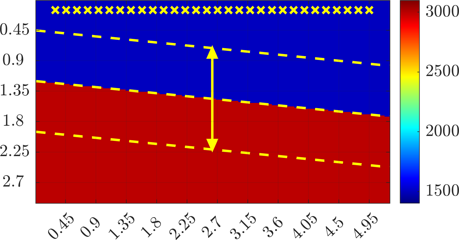
Log of FWI objective $\mathcal{O}^{\scalebox{0.5}[0.4]{FWI}}$	Log of ROM objective $\mathcal{O}^{\scalebox{0.5}[0.4]{ROM}}$

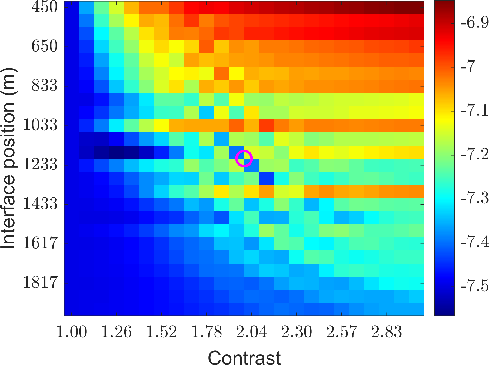
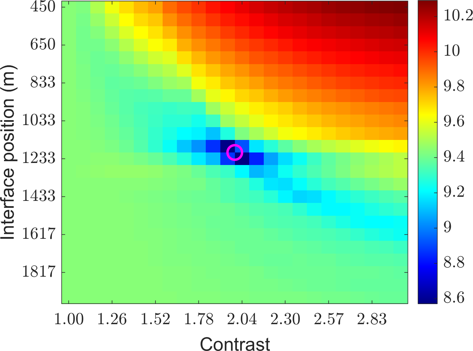
Figure 1: Top: velocity model for objective topography study. Middle dashed line shows the actual interface location; top and bottom dashed lines show the extent of interface location parameter sweep. All $m=30$ sensors are shown as yellow $\times$. Distances are in $\rm{km}$, velocity in $\rm{m/s}$. Bottom: logarithms of objective functions. True parameters are indicated with ${\color[rgb]{1,0,1}\bigcirc}$.

Consider the velocity model displayed in Figure 1 consisting of two regions separated by a slanted interface with velocities $c_{t}=1500$m/s and $c_{b}=3000$m/s above and below the interface, respectively. To compare the objective functions, we sweep a two-parameter search space: the first parameter is the depth of the interface at its leftmost point (actual depth is $1.2\rm{km}$); the second parameter is the contrast $c_{b}/c_{t}$ (actual contrast is $2$).

In Figure 1 we compare the conventional FWI objective $\mathcal{O}^{\scalebox{0.5}[0.4]{FWI}}$ to wave operator ROM objective $\mathcal{O}^{\scalebox{0.5}[0.4]{ROM}}$. We observe that $\mathcal{O}^{\scalebox{0.5}[0.4]{FWI}}$ displays numerous local minima, at points in the search space that are far from the true one. The horizontal stripes in FWI objective plot are manifestations of cycle skipping. The wave operator ROM objective is smooth and has a single minimum, at the true depth and contrast. This confirms that the wave operator ROM misfit minimization is superior to conventional FWI formulation for velocity estimation since $\mathcal{O}^{\scalebox{0.5}[0.4]{ROM}}$ is more friendly towards local optimization algorithms.

3.2 The “Camembert” example

Following Yang et al., (2018) we consider the “Camembert” model with a circular inclusion of radius of $600$m, centered at $(1\rm{km},1\rm{km})$ in $\Omega=[0,2\rm{km}]\times[0,2.5\rm{km}]$, with $c({{\itbf x}})=4000\rm{m/s}$ in the inclusion and $c({{\itbf x}})=3000\rm{m/s}$ outside, see Figure 2. The search space ${\cal C}$ consists of $N=400$ Gaussian basis functions centered at the nodes of a $20\times 20$ uniform grid discretizing $\Omega$. A constant initial guess $c_{o}({{\itbf x}})=3000\rm{m/s}$ is used.

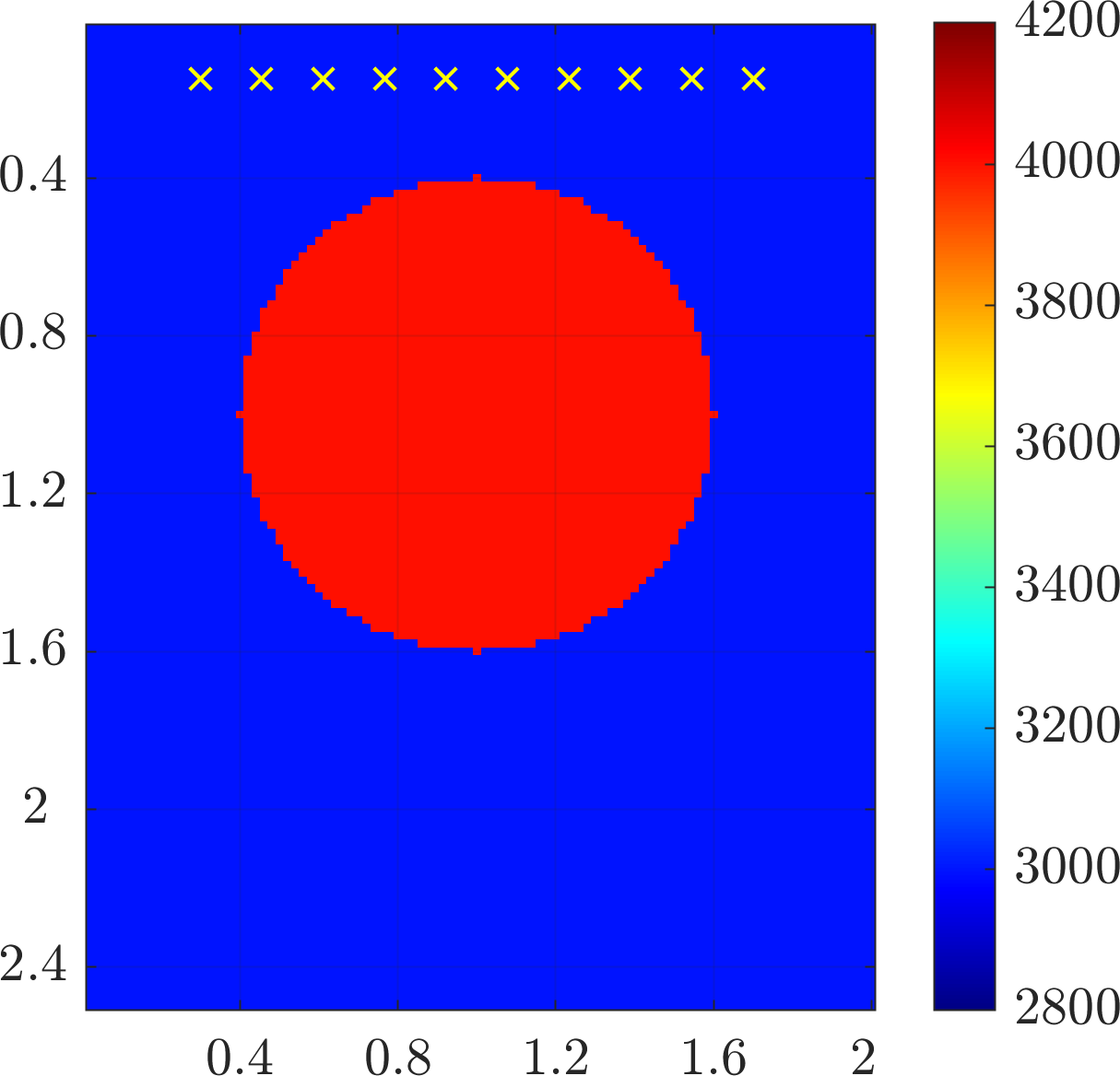
Operator ROM estimate	Conventional FWI estimate

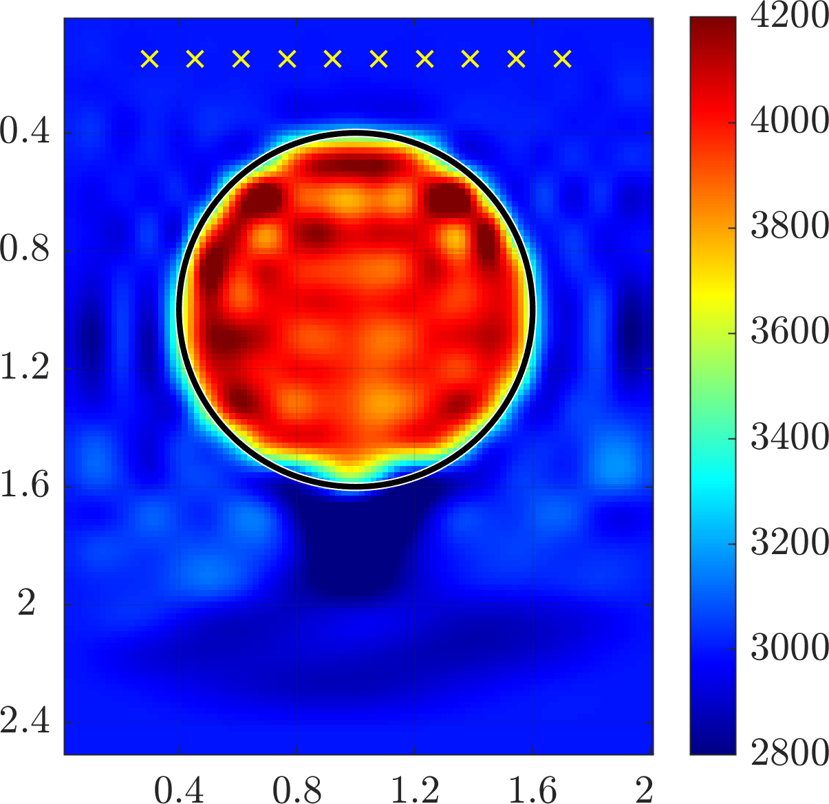
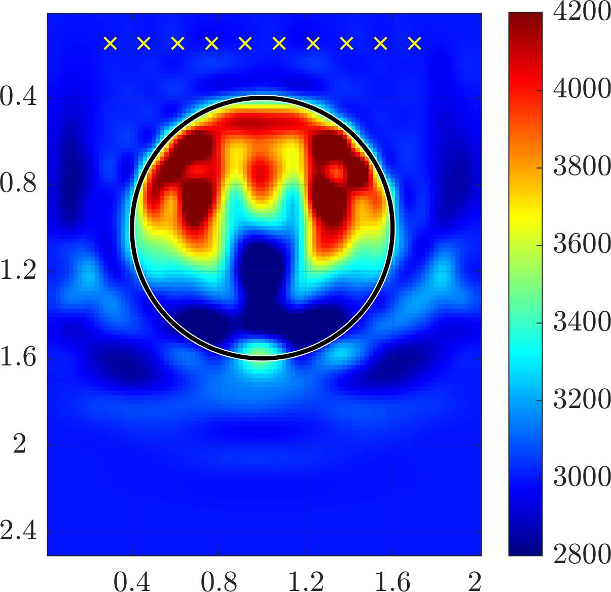
Figure 2: Top: “Camembert” velocity model. All $m=10$ sensors are shown as yellow $\times$. Bottom: estimated velocity after $60$ Gauss-Newton iterations, obtained with Algorithm 2 (left) and conventional FWI (right). True inclusion boundary is shown as a black circle. The axes are in $\rm{km}$, velocity in $\rm{m/s}$.

In the bottom row in Figure 2 we compare the velocity estimates obtained with Algorithm 2 (using parameters $L=9$, $q=4$, $d=n=16$) with conventional FWI regularized with adaptive Tikhonov regularization similarly to operator ROM approach, after performing $60$ Gauss-Newton iterations. We observe that Algorithm 2 gives a much better estimate of $c({{\itbf x}})$ that includes a correct reconstruction of both the top and bottom of the inclusion. Conventional FWI estimate does not improve much after the $10^{\rm th}$ iteration, indicating that it is stuck in a local minimum. Moreover, FWI fails to fill in the inclusion with the correct velocity, overestimating it in the upper half of the disk and underestimating it in the lower half.

3.3 Marmousi example

True velocity	FWI velocity estimate
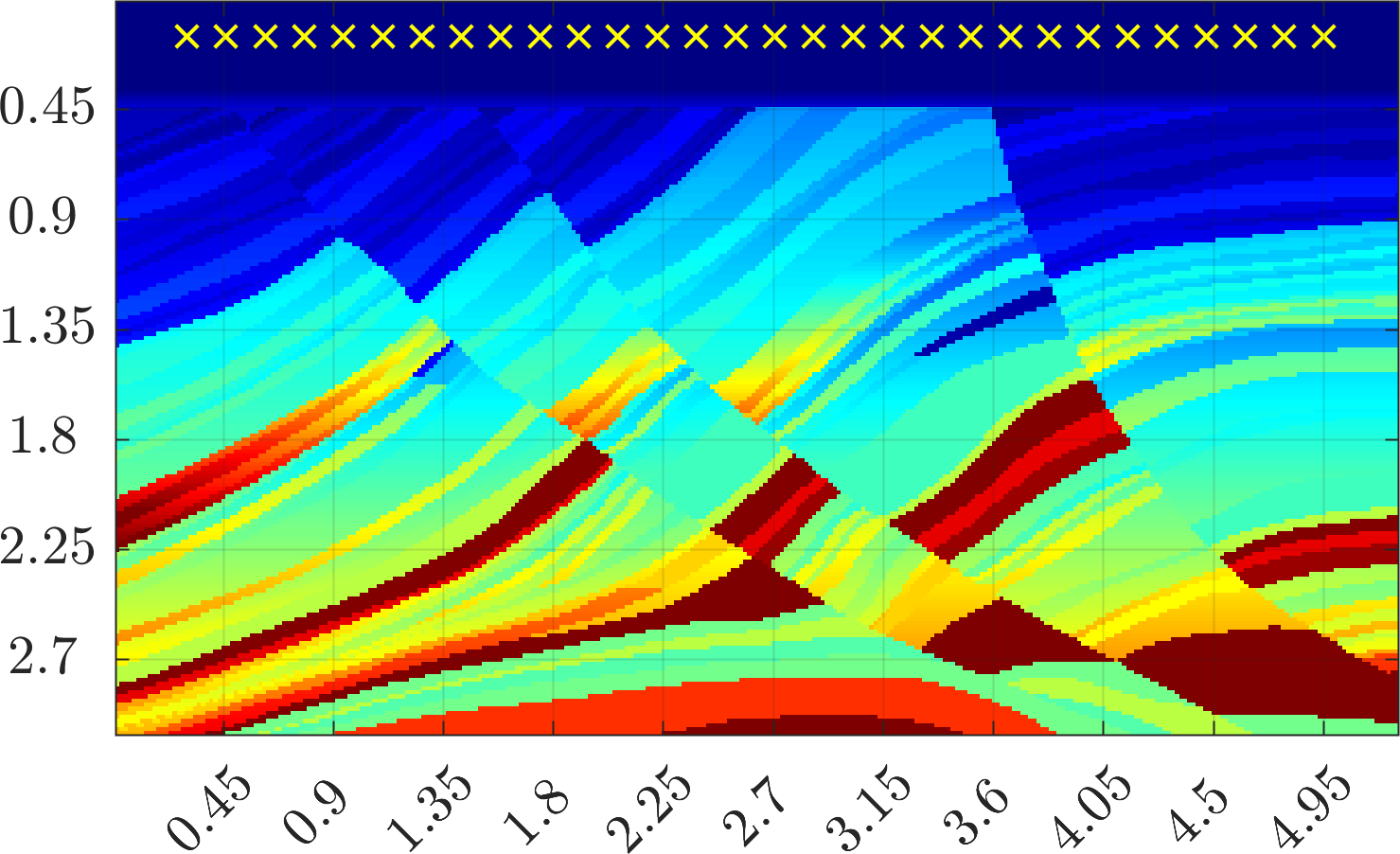
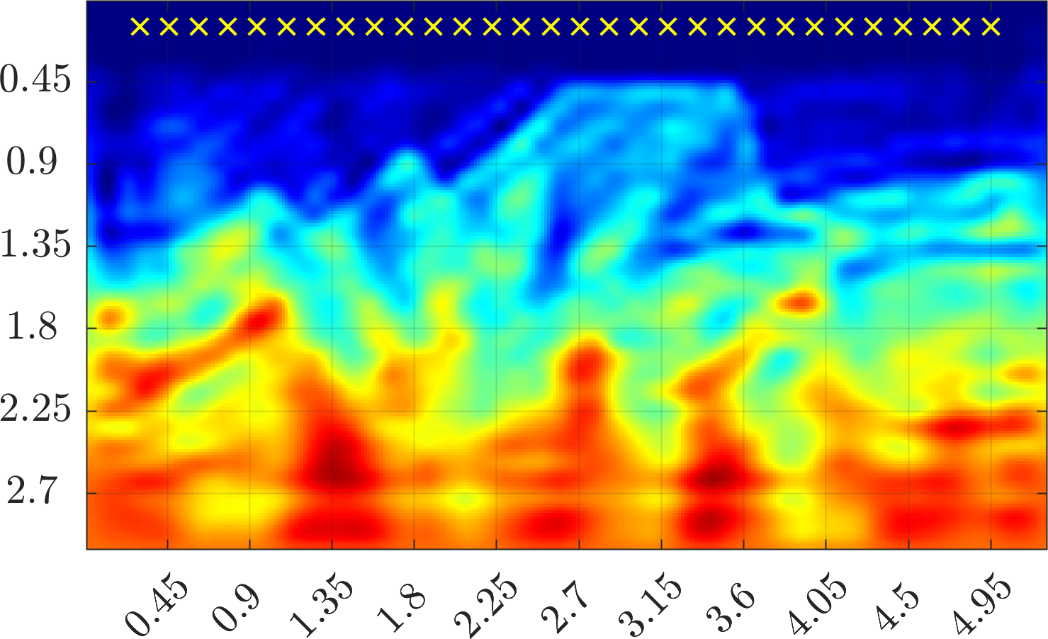
Refined ROM estimate	Operator ROM estimate

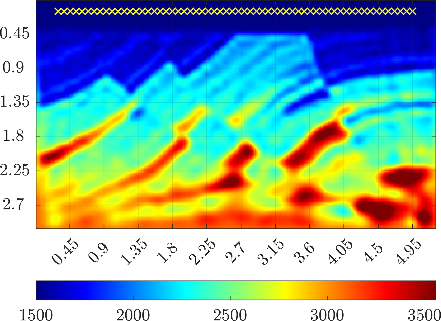
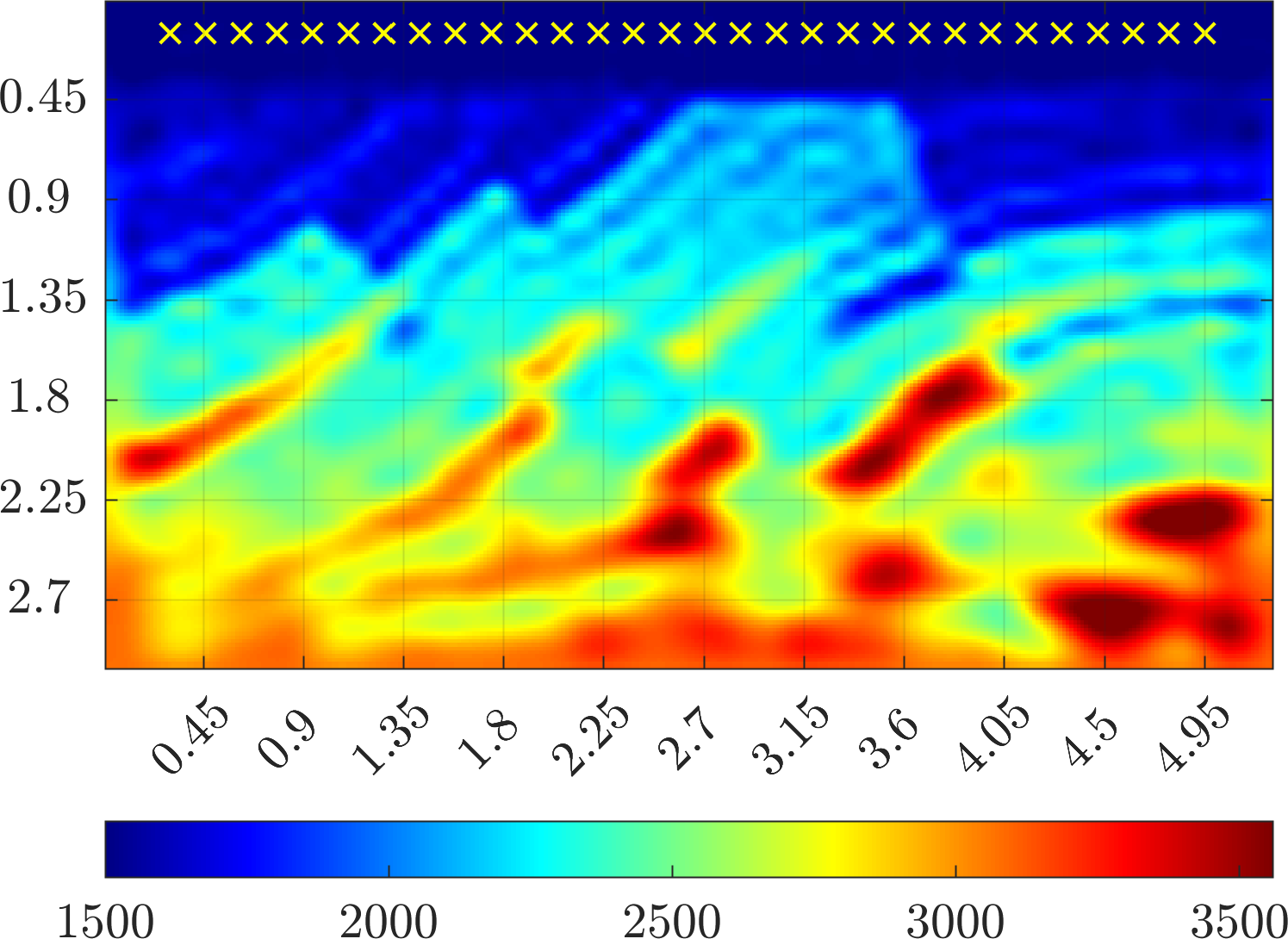
Figure 3: The section of Marmousi model (top left), velocity estimates obtained with Algorithm 2 (bottom row: left $m=60$, right $m=30$) and conventional FWI (top right, $m=30$). The sensors are shown as yellow $\times$. The axes are in $\rm{km}$, velocity in $\rm{m/s}$.

The final example is a section of Marmousi model with water layer down to depth $266{\rm m}$ removed. The domain is $\Omega=[0,5.25{\rm km}]\times[0,3{\rm km}]$. The search space ${\cal C}$ consists of $N=1500$ Gaussian basis functions centered at the nodes of a $50\times 30$ uniform grid discretizing $\Omega$. The initial guess $c_{o}({{\itbf x}})$ is a one dimensional gradient in depth.

In the right column of Figure 3 we compare the velocity estimates obtained from data recorded at $m=30$ sensors with Algorithm 2 (using parameters $L=6$, $q=3$, $d=10$, $n=40$) with conventional FWI regularized with adaptive Tikhonov regularization after $18$ Gauss-Newton iterations. We note that the ROM based inversion captures correctly most of the features of Marmousi model, while the conventional FWI velocity estimate suffers from a number of artifacts. We also display in the bottom left plot in Figure 3 a refinement of operator ROM velocity estimate obtained by injecting more data from $m=60$ sensors and performing $4$ additional Gauss-Newton iterations of Algorithm 2 (using parameters $L=1$, $q=4$, $d=10$, $n=50$) with a refined basis of $N=75\times 38=2850$ Gaussian functions. The resulting refined velocity estimate sharpens the boundaries of the features and improves their contrast.

4 Conclusions

We presented a novel approach for velocity estimation based on the wave operator ROM. The ROM is computed from the data and is used to formulate the optimization problem for velocity estimation as ROM misfit instead of the conventional FWI data misfit minimization. This has a convexification effect on the optimization objective, as shown in a numerical study of objective topography. As a result, the proposed approach outperforms the conventional FWI in synthetic examples such as the “Camembert” and Marmousi models.

5 ACKNOWLEDGMENTS

This material is based upon research supported in part by the U.S. Office of Naval Research under award number N00014-21-1-2370 to Borcea and Mamonov. Borcea, Garnier and Zimmerling also acknowledge support from the AFOSR awards FA9550-21-1-0166 and FA9550-22-1-0077. Zimmerling also acknowledges support from the National Science Foundation under Grant No. 2110265.

References

- Borcea et al., (2020) Borcea, L., V. Druskin, A. Mamonov, M. Zaslavsky, and J. Zimmerling, 2020, Reduced order model approach to inverse scattering: SIAM Journal on Imaging Sciences, 13, 685–723.
- Borcea et al., (2022) Borcea, L., J. Garnier, A. V. Mamonov, and J. Zimmerling, 2022, Waveform inversion via reduced order modeling: arXiv preprint arXiv:2202.01824.
- Druskin et al., (2018) Druskin, V., A. Mamonov, and M. Zaslavsky, 2018, A nonlinear method for imaging with acoustic waves via reduced order model backprojection: SIAM Journal on Imaging Sciences, 11, 164–196.
- Gauthier et al., (1986) Gauthier, O., J. Virieux, and A. Tarantola, 1986, Two-dimensional nonlinear inversion of seismic waveforms: Numerical results: Geophysics, 51, 1387–1403.
- Santosa and Symes, (1989) Santosa, F., and W. W. Symes, 1989, Analysis of least-squares velocity inversion: Society of exploration Geophysicists. Geophysical Monograph 4.
- Tarantola, (1984) Tarantola, A., 1984, Inversion of seismic reflection data in the acoustic approximation: Geophysics, 49, 1259–1266.
- Virieux and Operto, (2009) Virieux, J., and S. Operto, 2009, An overview of full-waveform inversion in exploration geophysics: Geophysics, 74, WCC1–WCC26.
- Yang et al., (2018) Yang, Y., B. Engquist, J. Sun, and B. Hamfeldt, 2018, Application of optimal transport and the quadratic wasserstein metric to full-waveform inversion: Geophysics, 83, R43–R62.