[font=]section

Bremsstrahlung from Neutrino Scattering via Magnetic Dipole Moments

Konstantin Asteriadis${}^{\,a,\,}$, Alejandro Quiroga Triviño${}^{\,b,\,c,\,}$ and Martin Spinrath${}^{\,b,\,c,\,d,\,}$

^aHigh Energy Theory Group, Physics Department,
Brookhaven National Laboratory, Upton, NY 11973, USA

^bDepartment of Physics, National Tsing Hua University, Hsinchu, 30013, Taiwan

^cPhysics Division, National Center for Theoretical Sciences, Taipei 10617, Taiwan

^dCenter for Theory and Computation, National Tsing Hua University, Hsinchu, 30013, Taiwan

Abstract

In this paper we discuss bremsstrahlung induced by neutrino scattering. This process should exist since neutrinos are expected to couple to photons via magnetic dipole and transition moments. These moments are loop-induced and tiny in the Standard Model with neutrino masses but could be significantly enhanced in extended theories. As concrete example we study the scattering of the two largest neutrino fluxes on earth, solar neutrinos and Cosmic Neutrino Background (CNB). It is tempting to consider this as a potential signature for CNB searches but it turns out that the signal is extremely small and unlikely to be observed.

1 Introduction

Neutrinos remain to be among the most fascinating particles due to their importance in particle physics, nuclear physics, astrophysics and cosmology. For instance, they are the only known particles with confirmed properties beyond the Standard Model of particle physics.

In cosmology one of their interesting aspects is that they form their own background, the Cosmic Neutrino Background (CNB), which is the equivalent to the Cosmic Microwave Background. The direct observation of the CNB in a laboratory remains one of the great challenges of experimental particle cosmology. Given the tiny cross sections and energies of CNB neutrinos it was even called an “apparently impossible experiment” [1]. Some recent proposals include detecting the tiny force induced by the CNB “wind” using current gravitational wave detector technology [2, 3], resonant scattering against ultra-high energetic cosmic neutrinos [4], cosmic birefringence induced by the CNB [5] and the absorption of CNB neutrinos on tritium [6, 7]. The last is probably the most promising proposal at this time, see, e.g., Refs. [8, 9, 10, 11] for more comprehensive reviews.

The original motivation for this work was to study an alternative method for its detection.

The idea is to look for a signature of the scattering between the two largest natural neutrino fluxes on earth: solar neutrinos and CNB neutrinos. Since the scattered neutrinos would still be hard to detect, we consider an additional bremsstrahlung photon in the final state that is comparatively easy to detect and that can be produced at any energy. To our knowledge, this is the first time this process was calculated. In other cases neutrinos were considered as the final states of the bremsstrahlung itself, i.e., [12, 13] and references therein.

In the Standard Model of particle physics (SM) including Dirac neutrino masses neutrinos couple to photons via loop induced magnetic dipole moments. The neutrino magnetic moment is tiny and so is the cross section for the considered process. For Majorana neutrinos, however, the magnetic moment is exactly zero. In this case, the scattering cross section is still non-zero if one considers transition magnetic moments, see, e.g. Ref. [14], and we expect the cross sections to be similar to the (simpler) Dirac case. In any case, this process should exist even in the SM and lead to a tiny photon flux throughout the universe. Nevertheless, as we will see the event rate for this process is extremely small and an observation of this photon flux seems rather unlikely even under optimistic assumptions. Although there might be extreme environments with large fluxes of high-energetic neutrinos where the considered process might become interesting.

2 Bremsstrahlung from
neutrino-neutrino scattering

We study the processes

$$\nu_{\odot}\;+\stackrel{{\scriptstyle\scalebox{0.3}{(}\raisebox{-1.7pt}{--}\scalebox{0.3}{)}}}{{\nu}}_{\text{CNB}}\to\nu\;+\stackrel{{\scriptstyle\scalebox{0.3}{(}\raisebox{-1.7pt}{--}\scalebox{0.3}{)}}}{{\nu}}+\;\gamma$$ (1)

at leading order, neglecting the exchanged momentum with respect to the $Z$-boson mass in the propagators, see also the Appendix for more details. Here $\nu_{\odot}$ is a solar neutrino and $\nu_{\text{CNB}}$ and $\bar{\nu}_{\text{CNB}}$ are relic neutrinos and anti-neutrinos, respectively. In the SM and standard cosmology the CNB is expected to consist of neutrinos and anti-neutrinos to equal parts and we assume neutrinos to be left-helical and anti-neutrinos to be right-helical today, cf. Ref. [15]. The solar neutrinos are assumed to be purely left-chiral and for the sake of simplicity we will neglect any flavor effects to get an estimate of the rate of these processes. We will comment later on how a more realistic flavor treatment can modify our results. To that end, we treat solar and CNB neutrinos to consist of only one flavor. We set the neutrino mass to be $m_{\nu}=0.05$ eV which is a mass scale compatible with current limits [16]. For that scale the CNB neutrinos are non-relativistic and we can neglect their velocity in our calculations. Interestingly though, non-vanishing CNB velocities would lead to corrections which would, in principle, allow to measure their velocity distribution.

In our setup, the photons couple to the neutrinos via an effective magnetic dipole moment with the effective Lagrangian [18]

$$\mathcal{L}_{\text{eff}}=-\operatorname{\text{i}}M_{\nu}\,\bar{\nu}\,\sigma_{\alpha\beta}\,q^{\alpha}\nu\,A^{\beta}\;,$$ (2)

where $\sigma_{\alpha\beta}$ is the anti-symmetric combination of $\gamma$-matrices, $q^{\alpha}$ is the momentum carried away by the photon field $A^{\beta}$, and $M_{\nu}$ is the magnetic moment of the neutrino. In general, $M_{\nu}$ is a matrix in flavor space. Since we do a one-flavor approximation $M_{\nu}$ is just a dimensionful number. The coupling then reads

$$\vbox{\hbox{\includegraphics[scale={.41},trim=25.09373pt 0.0pt 0.0pt 0.0pt,clip]{nna}}}\widehat{=}\hskip 7.0pt-\frac{\operatorname{\text{i}}}{2}(\gamma_{\beta}\not{q}-\not{q}\gamma_{\beta})M_{\nu}\;.$$ (3)

In the SM the coupling Eq. (3) occurs for Dirac neutrinos via loops with an effective coupling constant of $M_{\nu}^{\textrm{SM}}\lesssim 3.8\times 10^{-19}\mu_{B}$ [18]. Here we assume it to be additionally enhanced by some new physics. The parameter $M_{\nu}$ has been recently constrained by XENONnT to be $M_{\nu}<6.4\times 10^{-12}\,\mu_{B}$ at 90% CL [17]. In the following, we write $M_{\nu}=f_{M}\times 10^{-12}\,\mu_{B}$ for some $f_{M}\lesssim 6.4$. The total rate within our assumptions is proportional to $|f_{M}|^{2}$ which makes it easy to rescale our results to the true value of $M_{\nu}$. Note that, for Majorana neutrinos $f_{M}=0$, but considering multiple flavors and transition magnetic moments instead would also imply the existence of the considered process with expected results similar to the case of Dirac neutrinos.

Neutrinos can also have other electromagnetic moments. For instance, they could have a tiny electric charge. However, the current upper bound is so low that these contributions should be orders of magnitude smaller (even considering possible enhancements close to infrared singularities). For this reason, and for simplicity, we will neglect such complications here.

For this set of assumptions, the relation between the differential cross sections for CNB neutrinos $\sigma_{\nu\nu}$ and CNB anti-neutrinos $\sigma_{\nu\bar{\nu}}$ and the differential photon production rate $\textrm{d}R$ can be estimated as

$$\begin{split}\textrm{d}R&=n_{\text{CNB}}\int\textrm{d}E_{\nu}\\ &\hphantom{{}={}}\times\frac{\operatorname{\text{d}}\Phi_{\odot}}{\operatorname{\text{d}}E_{\nu}}\,\big{[}\textrm{d}\sigma_{\nu\nu}{(E_{\nu})}+\textrm{d}\sigma_{\nu\bar{\nu}}{(E_{\nu})}\big{]}\;,\end{split}$$ (4)

where the local CNB density is chosen to be $n_{\text{CNB}}=f_{n}\times 168$/cm³. For $f_{n}=1$ this density corresponds to the SM prediction. The factor $f_{n}$ parametrizes potential overdensities which are nevertheless not expected to be very large, see, e.g. Ref. [20]. The scaling factor $f_{n}$ can also depend on the neutrino flavor. Finally, $\operatorname{\text{d}}\Phi_{\odot}/\operatorname{\text{d}}E_{\nu}$ are the differential solar neutrino fluxes which have some energy-dependent flavor dependence in reality due to neutrino oscillations.

In our calculations we consider a target volume of 1 km³, at an earth-like distance from the sun. It is considered isolated from the surroundings while CNB and solar neutrinos can still enter and interact inside the volume. We calculate how many photons are produced in it within a year and how their energies and angles are distributed. The inner surface of the volume could be covered with suitable photon detectors but we do not want to go into further experimental and technical details which are beyond the scope of our theoretical work.

Numerical tables for the solar neutrino fluxes are taken from Ref. [21]. The final state phase space integration is performed numerically and getting the desired distributions is straightforward.

3 Results

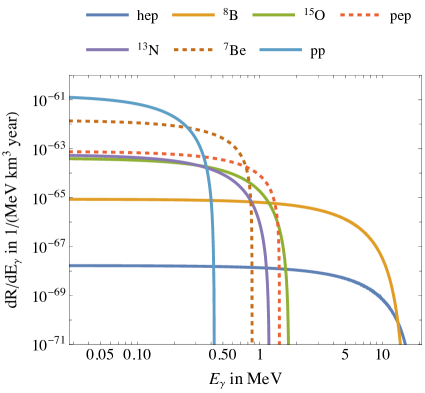
Figure 1: Energy distributions of the emitted bremsstrahlung photons. Here we have set $f_{M}=f_{n}=1$ and we separate the different components of the solar neutrino flux.

For numerical results reported in this section, we set $f_{M}=f_{n}=1$ and use $G_{F}=1.1663787\times 10^{-5}\,\textrm{GeV}^{-2}$ for the Fermi coupling constant and $\mu_{B}=296.238\,\textrm{GeV}^{-1}$ for the Bohr magneton.

In Fig. 1 we show the energy distribution of the emitted bremsstrahlung photons, separating the different components of the solar neutrino flux. It follows from this figure that they could be theoretically distinguished from each other. This is quite a unique feature which could potentially be used to separate the bremsstrahlung photons of this process from other potential backgrounds. We also see that the higher energies of the ⁸B and the hep neutrinos, implying larger cross sections, cannot compensate for the much larger flux of the pp neutrinos. We checked numerically that in the relevant energy range the cross section grows quadratically with the incoming neutrino energy to a good approximation. This increase is much weaker than the flux decrease for the high energy solar neutrinos. For that reason we also do not consider other naturally occurring neutrino fluxes such as atmospheric neutrinos which are much smaller than the solar flux [21].

The energy spectrum can be affected by flavor effects. First of all, the endpoints of the spectra depend on the actual neutrino masses which is a tiny effect considering the size of the neutrino masses compared to the photon energies near the endpoint. Furthermore, the solar neutrino flux has an energy dependent flavor composition which together with a non-trivial flavor structure of the dipole moments matrix might have a larger effect on, e.g., the shape of the energy distribution but is not expected to give an overall strong enhancement. Therefore we chose to keep the discussion of flavor effects simplistic in this work to get a first estimate of the size of this process.

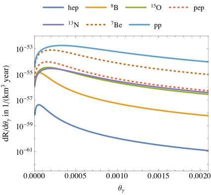
Figure 2: Angular distribution of the emitted bremsstrahlung photons. The angle is chosen such that $\theta_{\gamma}=0$ points away from the sun which is treated as a point source. Here we have set $f_{M}=f_{n}=1$.

In Fig. 2 we show the angular distribution with respect to the direction towards the center of the sun, assuming the incoming neutrino momenta to be parallel. As expected the distributions peak at $\theta_{\gamma}$ very close to zero. which is due to the “fixed target” nature of our setup and the very large energies of the incoming neutrinos compared to the target neutrino mass. This is another feature which could, in principle, be used to distinguish a signal from potential background photons. The width of the angular distribution is similar to the deviations that would be induced by the neutrino production zones in the sun which have a similar angular diameter in the sky [22]. Therefore, a fully realistic treatment would widen the distribution somewhat but there would still be a very strong directional dependence.

We assumed a detector volume that is shielded from any photons from the surroundings. Even in this ideal case there should be other photons, for instance, from neutrino decays ($\nu_{i}\to\nu_{j}+\gamma$) or Bremsstrahlung from neutrinos scattering from residual matter in the considered volume ($\nu+X\to\nu+X+\gamma$). However, these processes have different energy and angular distributions than the considered process and are therefore distinguishable in theory.

What becomes apparent from both figures is that the expected rates are extremely small. In fact, the total expected rate is about $2.1\times 10^{-56}$ bremsstrahlung photons per year and km³ of target volume assuming no neutrino overdensities and a neutrino magnetic dipole moment slightly below the current bound, to be precise $f_{M}=f_{n}=1$. That makes the discovery prospects of the CNB using this signature rather unlikely as one would need a neutrino beam with significantly higher energies, flux and/or observed volume to get a reasonable rate. Even if we consider a target volume as large as the earth covered with photon detector the rate is still of the order of $10^{-42}$ photons per year. Without the enhancement by new physics this number drops by an additional fourteen orders.

The dependence of the rate on the model parameters $f_{M}$ and $f_{n}$ is only quadratic and linear, respectively. Increasing the rate by orders of magnitude would also require increasing these parameters by orders of magnitudes which is not expected neither from experiments nor simulations.

What might be more promising to improve the rate is to increase the neutrino flux. Given that the biggest neutrino flux on earth are the CNB neutrinos themselves, self-scattering of CNB neutrinos may be an option. Such a process with similar kinematics to the process studied above would be a massless neutrino flavor scattering from a massive one. We can provide a rough estimate for this case. The flux would be roughly a factor 25 larger than the solar neutrino flux. On the other hand the cross section would drop by a factor $m_{\nu}^{2}/E_{\odot}^{2}\approx 2.5\times 10^{-15}$ where we used for the neutrino mass $m_{\nu}=0.05$ eV and for the solar neutrino energy $E_{\odot}\approx 10^{6}$ eV. This estimate is only an upper bound because the neutrino mass is used as the energy scale of the CNB self-scattering process instead of the much smaller kinetic energy. We conclude from the above numbers that this process would be even more rare compared to the one involving solar neutrinos. This said, this little thought experiment shows how the rates for other sources can be estimated as long as the center of mass energy is below the $Z$-boson mass and no other new physics scenarios are considered.

4 Conclusions

In this work we calculated for the first time the rate of bremsstrahlung photons produced in neutrino scattering. As concrete example we consider the two largest neutrino fluxes on earth, the solar neutrino flux and CNB neutrinos. Although we chose for our numerical results a magnetic dipole moment which is strongly enhanced compared to the SM and just slightly below the current experimental bound, the obtained cross section and rate is still tiny and somewhat discouraging for any experimental efforts in an earthbound laboratory in that direction. Notwithstanding, this process exists even in the SM and should generate a minuscule photon flux throughout the universe. While our original motivation was to study another way to detect the CNB our proposal fails in that regard and rather serves as a showcase how difficult that endeavour is.

We also showed how the bremsstrahlung photon rate for other energetic neutrino sources can be easily estimated assuming a similar set of assumptions. Other neutrino beams or sources, non-standard cosmology, additional new physics contributions, a larger target volume and a combination thereof could lead to a rate closer to being measurable. In particular, if it would not involve CNB neutrinos. We leave the study of these cases for further investigations.

Appendix: Details on the Cross Section Calculation

We give here the explicit expressions for the matrix elements of the considered processes. We consider a one-flavor approximation of Dirac neutrinos and only neutrino magnetic dipole moments are taken into account. We furthermore neglect the exchanged momentum in the $Z$-boson propagator.

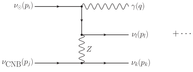
Figure 3: Example Feynman diagram for the bremsstrahlung emission from neutrino-neutrino scattering. We assume in this paper that the photons couple to neutrinos via a magnetic dipole moment, cf. Eq. (3). There are seven more diagrams. Three more diagrams where the photon couples to the other neutrino lines and four more where the indices $k$ and $l$ are interchanged. The latter four would not contribute for different neutrino flavors in the final state.

For the process involving only neutrinos, cf. Fig. 3,

$$\nu_{\odot}(p_{i})+\nu_{\text{CNB}}(p_{j})\to\nu(p_{k})+\nu(p_{l})+\gamma(q)\;,$$ (5)

we find the for the spin-averaged, squared amplitude

$$\frac{|\mathcal{M}(\nu\nu\to\nu\nu\gamma)|^{2}}{128\,G_{F}^{2}\,M_{\nu}^{2}}=6\,(p_{i}\cdot p_{j})(p_{k}\cdot p_{l})$$

$$+m_{\nu}^{2}\biggl{[}2\,(p_{i}\cdot p_{l})+2\,(p_{i}\cdot p_{k})-4\,(p_{i}\cdot p_{j})$$

$$+(p_{j}\cdot p_{l})+(p_{j}\cdot p_{k})-2\,(p_{k}\cdot p_{l})$$

$$-\frac{(p_{i}\cdot p_{k})(p_{j}\cdot q)}{(p_{i}\cdot q)}-\frac{(p_{i}\cdot p_{l})(p_{j}\cdot q)}{(p_{i}\cdot q)}$$

$$+\frac{(p_{j}\cdot q)(p_{k}\cdot p_{l})}{(p_{i}\cdot q)}-2\frac{(p_{i}\cdot q)(p_{j}\cdot p_{k})}{(p_{j}\cdot q)}$$

$$-2\frac{(p_{i}\cdot q)(p_{j}\cdot p_{l})}{(p_{j}\cdot q)}-2\frac{(p_{i}\cdot p_{k})(p_{l}\cdot q)}{(p_{k}\cdot q)}$$

$$-\frac{(p_{j}\cdot p_{k})(p_{l}\cdot q)}{(p_{k}\cdot q)}-2\frac{(p_{i}\cdot p_{l})(p_{k}\cdot q)}{(p_{l}\cdot q)}$$

$$-\frac{(p_{j}\cdot p_{l})(p_{k}\cdot q)}{(p_{l}\cdot q)}+\frac{(p_{i}\cdot p_{k})(p_{j}\cdot q)(p_{l}\cdot q)}{(p_{i}\cdot q)(p_{k}\cdot q)}$$

$$+\frac{(p_{i}\cdot p_{l})(p_{j}\cdot q)(p_{k}\cdot q)}{(p_{i}\cdot q)(p_{l}\cdot q)}$$

$$+2\frac{(p_{i}\cdot q)(p_{j}\cdot p_{k})(p_{l}\cdot q)}{(p_{j}\cdot q)(p_{k}\cdot q)}$$

$$+2\frac{(p_{i}\cdot q)(p_{j}\cdot p_{l})(p_{k}\cdot q)}{(p_{j}\cdot q)(p_{l}\cdot q)}\biggr{]}\;,$$ (6)

where we have used four momentum conservation and the on-shell conditions $q^{2}=0$ and $p_{i}^{2}=p_{j}^{2}=p_{k}^{2}=p_{l}^{2}=m_{\nu}^{2}$. $M_{\nu}$ is the magnetic dipole moment of the neutrino and $G_{F}$ is the Fermi constant.

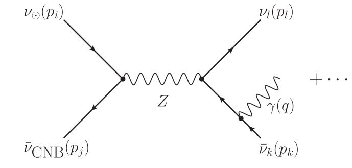
Figure 4: Example Feynman diagram for the Bremsstrahlung emission from neutrino-antineutrino scattering. We assume in this paper that the photons couple to neutrinos and antineutrinos via a magnetic dipole moment, cf. Eq. (3). There are seven more diagrams. Three more diagrams where the photon couples to the other neutrino and anti-neutrino lines and four more similar to the diagram in Fig. 3. The diagrams similar to the one shown in this figure would not contribute for different neutrino flavors in the initial state.

For the process involving anti-neutrinos, cf. Fig. 4,

$$\nu_{\odot}(p_{i})+\bar{\nu}_{\text{CNB}}(p_{j})\to\nu(p_{k})+\bar{\nu}(p_{l})+\gamma(q)\;,$$ (7)

we find

$$\frac{|\mathcal{M}(\nu\bar{\nu}\to\nu\bar{\nu}\gamma)|^{2}}{128\,G_{F}^{2}\,M_{\nu}^{2}}=6\,(p_{i}\cdot p_{l})(p_{j}\cdot p_{k})$$

$$+m_{\nu}^{2}\Biggl{(}2\,(p_{i}\cdot p_{k})-2\,(p_{i}\cdot p_{j})+4\,(p_{i}\cdot p_{l})$$

$$+2\,(p_{j}\cdot p_{k})+(p_{j}\cdot p_{l})-(p_{k}\cdot p_{l})$$

$$-\frac{(p_{i}\cdot p_{j})(p_{l}\cdot q)}{(p_{i}\cdot q)}+\frac{(p_{i}\cdot p_{k})(p_{l}\cdot q)}{(p_{i}\cdot q)}$$

$$+\frac{(p_{j}\cdot p_{k})(p_{l}\cdot q)}{(p_{i}\cdot q)}-2\frac{(p_{i}\cdot p_{j})(p_{k}\cdot q)}{(p_{j}\cdot q)}$$

$$+\frac{(p_{j}\cdot p_{l})(p_{k}\cdot q)}{(p_{j}\cdot q)}+\frac{(p_{i}\cdot p_{k})(p_{j}\cdot q)}{(p_{k}\cdot q)}$$

$$-\frac{(p_{j}\cdot q)(p_{k}\cdot p_{l})}{(p_{k}\cdot q)}+2\frac{(p_{i}\cdot q)(p_{j}\cdot p_{l})}{(p_{l}\cdot q)}$$

$$-2\frac{(p_{i}\cdot q)(p_{k}\cdot p_{l})}{(p_{l}\cdot q)}-\frac{(p_{i}\cdot p_{j})(p_{k}\cdot q)(p_{l}\cdot q)}{(p_{i}\cdot q)(p_{j}\cdot q)}$$

$$+\frac{(p_{i}\cdot p_{k})(p_{j}\cdot q)(p_{l}\cdot q)}{(p_{i}\cdot q)(p_{k}\cdot q)}$$

$$+2\frac{(p_{i}\cdot q)(p_{j}\cdot p_{l})(p_{k}\cdot q)}{(p_{j}\cdot q)(p_{l}\cdot q)}$$

$$-2\frac{(p_{i}\cdot q)(p_{j}\cdot q)(p_{k}\cdot p_{l})}{(p_{k}\cdot q)(p_{l}\cdot q)}\Biggr{)}\;.$$ (8)

In both cases, the matrix element decomposes into a part which is proportional to the neutrino scattering case without additional photon, e.g., $|\mathcal{M}(\nu\nu\to\nu\nu)|^{2}=64\,G_{F}^{2}(p_{i}\cdot p_{j})(p_{k}\cdot p_{l})$, and a part suppressed by neutrino masses.

In most cases, the matrix element is well approximated by the first term. Only in the very forward direction for small scattering angles, the denominators in the suppressed term can become of order $m_{\nu}^{2}$ and they become of similar importance.

With the matrix elements at hand, we can calculate the actual cross section used in Eq. (4)

$$\begin{split}\textrm{d}\sigma_{\nu\nu}{(E_{\nu}=E_{i})}&=\frac{1}{(2\,\pi)^{5}}\int\frac{\operatorname{\text{d}}^{3}p_{k}}{2\,E_{k}}\frac{\operatorname{\text{d}}^{3}p_{l}}{2\,E_{l}}\frac{\operatorname{\text{d}}^{3}q}{2\,E_{\gamma}}\\ &\times\frac{|{\cal M}(\nu\nu\to\nu\nu\gamma)|^{2}}{4\sqrt{(p_{i}\cdot p_{j})^{2}-m_{\nu}^{4}}}\\ &\times\delta^{4}(p_{i}+p_{j}-p_{k}-p_{l}-q)\;,\end{split}$$ (9)

and for $\textrm{d}\sigma_{\nu\bar{\nu}}$ we just replace the matrix element. The calculation of the phase space is difficult analytically and we performed it numerically at the same time with the integration over the energy spectrum of the incoming solar neutrinos to produce the distributions in Figs. 1 and 2.

Actually, we can use the results for the matrix elements to provide a rough estimate for the cross section which is supported by our numerical results. Ignoring the small terms proportional to neutrino masses the momentum structure is the same as for ordinary neutrino scattering which has a cross section of the order of

$$\sigma_{2}\sim\frac{G_{F}^{2}}{4\,\pi}s\;.$$ (10)

Now in our case we need to get an additional factor $M_{\nu}^{2}$ from the coupling to the photon which has units of inverse mass squared. Since the momenta in the matrix elements are all taken care of already by $\sigma_{2}$ we can only compensate it by the neutrino masses. Hence, we can guess the order of the cross section to be

$$\sigma\sim\frac{G_{F}^{2}}{4\,\pi}\frac{M_{\nu}^{2}}{4\,\pi}m_{\nu}^{2}\,s\approx 7.4\times 10^{-93}\,f_{M}^{2}\text{ cm}^{2}\;.$$ (11)

To get the rate we multiply this with the total solar neutrino flux on earth $\Phi_{\odot}\approx 10^{11}$ cm^-2 s^-1 and the total relic neutrino number density $n_{\nu}\approx f_{n}\times 300$ cm^-3 to get

$$R\approx 7.0\times 10^{-57}\,f_{n}\,f_{M}^{2}\frac{1}{\text{km}^{3}\text{ year}}\;.$$ (12)

This is actually close to our true value of $R\approx 2.1\times 10^{-56}\,f_{n}\,f_{M}^{2}$ km^-3 year^-1.

While this estimate is quite simple, we want to emphasize that we can only trust it since it is backed by our full calculation. For instance, if the cross section would scale with $s^{2}$ or $m_{\nu}^{4}$ instead, we would get completely different results which justifies the detailed calculations discussed in the main text.

Nevertheless, should a reader consider this process in a different context the simple estimate presented here might be useful to get a rough idea of the expected rates.

References

- [1] A. C. Melissinos, Contribution to Conference on Probing Luminous and Dark Matter: Adrian Fest (1999), 262-285.
- [2] V. Domcke and M. Spinrath, JCAP 06 (2017), 055 [arXiv:1703.08629 [astro-ph.CO]].
- [3] J. D. Shergold, JCAP 11 (2021) no. 11, 052 [arXiv:2109.07482 [hep-ph]].
- [4] V. Brdar, P. S. B. Dev, R. Plestid and A. Soni, Phys. Lett. B 833 (2022), 137358 [arXiv:2207.02860 [hep-ph]].
- [5] R. Mohammadi, J. Khodagholizadeh, M. Sadegh, A. Vahedi and S. S. Xue, [arXiv:2109.00152 [hep-ph]].
- [6] E. Baracchini et al. [PTOLEMY], [arXiv:1808.01892 [physics.ins-det]].
- [7] S. Betts et al., [arXiv:1307.4738 [astro-ph.IM]].
- [8] G. B. Gelmini, Phys. Scripta T 121 (2005), 131-136 [arXiv:hep-ph/0412305 [hep-ph]].
- [9] A. Ringwald, Nucl. Phys. A 827 (2009), 501C-506C [arXiv:0901.1529 [astro-ph.CO]].
- [10] P. Vogel, AIP Conf. Proc. 1666 (2015) no. 1, 140003.
- [11] M. Bauer and J. D. Shergold, JCAP 01 (2023), 003 [arXiv:2207.12413 [hep-ph]].
- [12] S. Hannestad and G. Raffelt, Astrophys. J. 507 (1998), 339-352 [arXiv:astro-ph/9711132 [astro-ph]].
- [13] I. Bhattacharyya, J. Phys. G 32 (2006), 2167-2180 [arXiv:hep-ph/0512107 [hep-ph]].
- [14] M. Czakon, J. Gluza and M. Zralek, Phys. Rev. D 59 (1999), 013010
- [15] A. J. Long, C. Lunardini and E. Sabancilar, JCAP 08 (2014), 038 [arXiv:1405.7654 [hep-ph]].
- [16] R. L. Workman et al. [Particle Data Group], PTEP 2022 (2022), 083C01
- [17] E. Aprile et al. [XENON], Phys. Rev. Lett. 129 (2022) no.16, 161805 [arXiv:2207.11330 [hep-ex]].
- [18] C. Giunti and A. Studenikin, Rev. Mod. Phys. 87 (2015), 531 [arXiv:1403.6344 [hep-ph]].
- [19] P. A. Zyla et al. [Particle Data Group], PTEP 2020 (2020) no. 8, 083C01.
- [20] A. Ringwald and Y. Y. Y. Wong, JCAP 12 (2004), 005 [arXiv:hep-ph/0408241 [hep-ph]].
- [21] E. Vitagliano, I. Tamborra and G. Raffelt, Rev. Mod. Phys. 92 (2020), 45006 [arXiv:1910.11878 [astro-ph.HE]].
- [22] G. L. Lin, T. T. L. Nguyen, M. Spinrath, T. D. H. Van and T. C. Wang, JCAP 08 (2022), 027 [arXiv:2201.06733 [hep-ph]].