The Effect of Omitted Variables on
the Sign of Regression Coefficients

Abstract

Omitted variables are a common concern in empirical research. We distinguish between two ways omitted variables can affect baseline estimates: by driving them to zero or by reversing their sign. We show that, depending on how the impact of omitted variables is measured, it can be substantially easier for omitted variables to flip coefficient signs than to drive them to zero. Consequently, results which are considered robust to being “explained away” by omitted variables are not necessarily robust to sign changes. We show that this behavior occurs with “Oster’s delta” (Oster 2019), a commonly reported measure of regression coefficient robustness to the presence of omitted variables. Specifically, we show that any time this measure is large—suggesting that omitted variables may be unimportant—a much smaller value reverses the sign of the parameter of interest. Relatedly, we show that selection bias adjusted estimands can be extremely sensitive to the choice of the sensitivity parameter. Specifically, researchers commonly compute a bias adjustment under the assumption that Oster’s delta equals one. Under the alternative assumption that delta is very close to one, but not exactly equal to one, we show that the bias can instead be arbitrarily large. To address these concerns, we propose a modified measure of robustness that accounts for such sign changes, and discuss best practices for assessing sensitivity to omitted variables. We demonstrate this sign flipping behavior in an empirical application to social capital and the rise of the Nazi party, where we show how it can overturn conclusions about robustness, and how our proposed modifications can be used to regain robustness. We analyze three additional empirical applications as well. We implement our proposed methods in the companion Stata module regsensitivity for easy use in practice.

JEL classification: C14; C18; C21; C25; C51

Keywords: Identification, Treatment Effects, Partial Identification, Sensitivity Analysis, Unconfoundedness

1 Introduction

The analysis of causality often relies on untestable assumptions, like the absence of unobserved omitted variables that could bias one’s findings. A large literature in statistics and econometrics now provides many tools that allow researchers to perform sensitivity analyses to assess the importance of these assumptions. Many of these methods use breakdown points as quantitative measures of the robustness of one’s conclusions to departures from the baseline identifying assumptions. These points tell us how much we can depart from our identifying assumptions before our empirical conclusions break down in some way.

In this paper, we distinguish between two specific kinds of breakdown points. The first is the explain away breakdown point. It answers the question

• What is the smallest value of the sensitivity parameter required for the data to be consistent with a zero causal effect?

The second is the sign change breakdown point. It answers the question

• What is the smallest value of the sensitivity parameter required for the data to be consistent with a causal effect that has a different sign from the causal effect we found in the baseline model?

In section 2 we show that these two breakdown points are in general not equivalent. In particular, we show that the sign change breakdown point can be smaller than the explain away breakdown point. Hence it can be easier to reverse the sign of your results than to drive them to zero. This can occur when the omitted variable bias is discontinuous in the sensitivity parameter, allowing the value of the bias adjusted estimand to jump across the horizontal axis at zero as the sensitivity parameter varies. This behavior is illustrated in figure 1, which we discuss more below. Such discontinuities can arise in regression analysis because the sensitivity parameters often involve covariance and variance terms, which lead to nonlinear restrictions on the value of the bias.

We discuss these ideas formally in section 2, in the context of a general model. In sections 3 and 4 we then apply them to study the specific sensitivity analysis of Oster (2019) (hereafter Oster), designed to assess the importance of omitted variables in regression analysis. This approach has been extremely influential, with about 3000 Google Scholar citations as of February 2023. Finkelstein et al. (2021, AER, page 2706) describe it as providing “the now-standard methodology” and “the standard approach” to adjusting for selection on unobservables. Moreover, from 2019–2021, 23 papers published in the top five economics journals formally compute and report the results from this method, while another 8 papers informally reference this method in support of their analysis. Based on the data collected by Blandhol et al. (2022), this is larger than the number of papers that use 2SLS per year, among papers published in top five economics journals. We discuss in detail how Oster’s (2019) results are used in empirical economics in section 7.

In section 3 we review Oster’s (2019) method. The main sensitivity parameter for this method, denoted by $\delta$, is commonly interpreted as the ratio of the magnitude of selection on unobservables to the magnitude of selection on observables. We then study breakdown points for this sensitivity parameter in section 4. Oster’s Proposition 2 characterizes the explain away breakdown point. Following her recommendation, empirical researchers now routinely report estimates of this explain away breakdown point as a measure of robustness to omitted variables. We show that this explain away breakdown point is very different from the sign change breakdown point. In fact, we show that any time the explain away breakdown point is large—suggesting that omitted variables may be unimportant—a much smaller value of her sensitivity parameter can actually change the sign of the parameter of interest. In particular, we prove that the sign change breakdown point is bounded above by $\delta=1$. This is a substantial concern since 1 is often viewed as the cutoff for a robust result. Consequently, if we maintain 1 as the cutoff, our result implies that no empirical results are robust to sign changes, using Oster’s method. Put differently: The true causal effect can have the opposite sign as the baseline estimand any time the magnitude of selection on unobservables is at least as large as the magnitude of selection on observables.

In section 5 we study selection bias adjusted estimands. We show that the most commonly used adjustment is extremely sensitive to perturbations of Oster’s sensitivity parameter. We also show that one of the key assumptions this adjustment relies on is testable and develop a simple hypothesis test for it. We conclude section 5 by explaining a common but incorrect approach to computing explain away breakdown points.

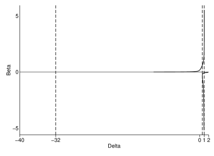
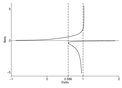
Figure 1: Example of Oster’s identified set $\mathcal{B}_{I}(\delta,R_{\text{long}}^{2})$ for the regression coefficient $\beta$ as a function of the sensitivity parameter $\delta$ (see section 3 for a definition of this set and a description of the $R_{\text{long}}^{2}$ parameter). As we discuss in section 3.3, this identified set always has either one, two, or three elements. Both plots show the same set, but with different horizontal axis ranges. In this example, the explain away breakdown point is $|-32|$. This is shown on the left plot. In contrast, the sign change breakdown point is 0.586, as shown in the right plot. The plot also shows the vertical asymptote at $\delta=1$ which we discuss in section 4.1.

To build intuition for our main results in section 4, consider figure 1. Both plots show the same curve, but with different horizontal axis ranges, to highlight different aspects which we discuss below. This curve is an example from our empirical application in section 6. It shows the pairs of regression coefficient values $\beta$ (on the vertical axis) and Oster’s main sensitivity parameter $\delta$ (on the horizontal axis) that are consistent with the data and assumptions. Importantly, as shown in the right plot, for some values of $\delta$ there are multiple values of $\beta$ that are consistent with the data. This occurs because $\delta$ is defined to be a ratio of two regression coefficients, and hence knowledge of $\delta$’s exact value implies that $\beta$ must satisfy a fairly complicated nonlinear constraint. Specifically, it must be the solution to a cubic equation (see Theorem 2), which can sometimes have multiple roots. This explains the source of the discontinuity in the value of the omitted variable bias that we discussed earlier, and why for this sensitivity parameter it is easier to flip the coefficient sign than to obtain an exact zero.

Concretely, in this example the baseline estimate is the vertical intercept at $\delta=0$. This estimate is positive. How robust is this estimate to the presence of omitted variables? In the left plot we see that we must go all the way to $\delta=-32$ before the value $\beta=0$ is consistent with the data and assumptions. This is the number that researchers commonly report as a measure of robustness. However, from the right plot, we see that we only need to go to $\delta=0.586$ to find a value of $\beta$ that is negative. This value $\delta=0.586$ is the sign change breakdown point. Oster (2019) does not discuss this breakdown point, the companion Stata package psacalc does not compute it, and none of the top five papers we survey in section 7 report it. Yet, as we see here, the sign change breakdown point is substantially smaller than $|-32|$, the explain away breakdown point. Indeed, it is below $\delta=1$, the commonly used cutoff for a robust result. Consequently, in this empirical example, focusing on the sign change breakdown point overturns the authors’ conclusion of robustness: Only a small amount of selection on unobservables relative to observables is necessary to flip the sign of the baseline estimate.

Figure 1 is also useful for building intuition for our results in section 5 on the sensitivity of bias adjustments. In the figure, we see there is an asymptote at $\delta=1$. This implies that bias adjustments computed at $\delta$ exactly equal to one—which is currently standard empirical practice—are not representative of bias adjustments computed at nearby values of $\delta$. This explains our discussion in section 5.5 on why Oster’s (2019) “bounding set” does not correctly represent the values of the regression coefficient consistent with any $\delta$ between 0 and 1. Importantly, all of the coefficient values plotted in figure 1, even the seemingly extreme values, are equally consistent with the data and assumptions. Under the assumptions of Oster’s Proposition 2 (see our Theorem 2), which is used to obtain these plots, there is no justification for ignoring any of these values. The only way to eliminate values is by making additional assumptions. One reasonable assumption, which we consider in section 4.2, is to restrict the magnitude of the omitted variable bias. With this additional assumption, we can justifiably eliminate some of the most extreme values. This assumption does not overturn our main conclusions, however. For example, in figure 1 the coefficient value consistent with $\delta=0.586$ is not extreme at all—it is the same order of magnitude as the baseline estimate. So in this example, the sign change breakdown point is still very different from the explain away breakdown point, even with a substantial restriction on the magnitude of the omitted variable bias. Moreover, magnitude restrictions require researchers to choose a tuning parameter—just how much should they restrict the magnitude? If the magnitude is restricted too much, then this assumption is essentially equivalent to assuming a priori that there is no omitted variable bias, in which case a sensitivity analysis would be unnecessary. But as soon as reasonably sized magnitudes are allowed, the concerns we discuss in sections 4 and 5 arise.

To address the issues described in sections 4 and 5, we propose several simple modifications to the methods in Oster (2019). First, we develop the sign change breakdown point for Oster’s main sensitivity parameter and recommend that researchers report this rather than, or in addition to, the explain away breakdown point. Second, to avoid the sensitivity inherent in the bias adjusted estimands, we recommend gathering all values of the coefficient consistent with a range of sensitivity parameters, and presenting this set. Furthermore, in section 4.2, we provide extensions to these two recommendations to formally incorporate the magnitude restrictions discussed above. We show that the sign change breakdown point can be strictly larger than 1 when a magnitude restriction is imposed. Therefore it is possible to recover findings of robustness even without changing the cutoff for robustness. This is not always the case however, as we saw in figure 1.

In section 6 we illustrate our results using data from Satyanath et al. (2017, Journal of Political Economy), who study the effect of social capital on the rise of the Nazi party. There we show just how different the sign change and explain away breakdown points can be in practice. We then show how magnitude restrictions can sometimes help retain findings of robustness. We also illustrate the extreme sensitivity of bias adjusted estimands to perturbations of the sensitivity parameter. In appendix A we analyze three additional empirical applications, all published in the American Economic Review. Finally, in section 8 we conclude with a discussion of best practices for regression sensitivity analysis.

Additional Technical Contribution

In section 3 we show that the set defined in Oster’s Proposition 2 is in fact sharp, with one minor technical caveat, and therefore equals the identified set under the assumptions of that proposition. In contrast, Oster (2019) only showed that this set was an outer set, containing the true identified set, but did not discuss whether this set was sharp. This sharpness result is important to ensure that Oster’s breakdown analysis is not unnecessarily conservative. Similarly, in section 5 we provide a proof that the result in Oster’s Proposition 1 is sharp.

Related Literature

A wide variety of papers propose methods for analyzing the sensitivity of regression based findings. This includes Mauro (1990), Murphy and Topel (1990), Frank (2000), Imbens (2003), Altonji et al. (2005), Clarke (2009), Bellows and Miguel (2009), Hosman et al. (2010), Gonzalez and Miguel (2015), Krauth (2016), Oster (2019), Cinelli and Hazlett (2020), and Diegert et al. (2022). Many other papers propose sensitivity analyses for nonlinear models, including Rosenbaum and Rubin (1983), Rosenbaum (1995, 2002), Robins et al. (2000), Altonji, Elder, and Taber (2005, 2008), Masten and Poirier (2018), and Altonji et al. (2019).

Our analysis primarily focuses on Oster’s (2019) approach, since it is by far the most popular method for regression sensitivity analysis in economics. That said, our distinction between explain away and sign change breakdown points in section 2 is more general, and therefore can be applied to other methods too. For example, Imbens (2003) studies a model of treatment effects which parameterizes deviations from conditional random assignment. Figures 1–4 in Imbens (2003) plot exact value breakdown curves (curves rather than points because he uses two sensitivity parameters). Because a similar asymptotic phenomenon as shown in our figure 1 occurs in Imbens’ model, these exact value breakdown curves do not capture sign changes. Thus the sign change and explain away breakdown points will generally be quite different in his model as well. As we discuss in section 2, a similar remark generally applies for any sensitivity analysis based on deviations rather than interval relaxations. One exception is Krauth (2016). Like Oster (2019), he starts with a deviation based analysis. His deviations also induce asymptotes (see his figure 1), but he generally works with a convex hull of the identified set (his equations 15 and 16) which ensures that explain away and sign change breakdown points are the same.

The general idea of an explain away type sensitivity analysis goes back to Cornfield et al. (1959). Sign change type breakdown analysis has also been studied before; for example, see the detailed literature review in Masten and Poirier (2020, section 1 and Appendix D). However, we are unaware of any previous papers that explicitly draw the distinction between explain away and sign change breakdown points, and emphasize how different they can be when one is using a deviation based sensitivity analysis.

Notation Remark

For random vectors $A$ and $B$, define $A^{\perp B}=A-[\operatorname*{var}(B)^{-1}\operatorname*{cov}(B,A)]^{\prime}B$. This is the sum of the residual from a linear projection of $A$ onto $(1,B)$ and the intercept in that projection.

2 Measuring Robustness: Sign Changes versus Explaining Away

In this section we formally define and analyze the two kinds of breakdown points discussed in section 1. We then apply this analysis in sections 3 and 4. Consider a model indexed by a scalar sensitivity parameter $r\geq 0$. We focus on the scalar case for simplicity; see Masten and Poirier (2020) for a study of breakdown analysis for vector relaxations. Let $\mathcal{B}_{I}(r^{*})\subseteq\mathbb{R}$ denote the identified set for the parameter of interest $\beta\in\mathbb{R}$ under the assumption $r=r^{*}$. Suppose $r=0$ represents the baseline model, while values $r>0$ represent alternative assumptions about the model.

Definition 1.

Say that $r$ represents a relaxation of the baseline model if $\mathcal{B}_{I}(r_{1})\subseteq\mathcal{B}_{I}(r_{2})$ for any $r_{1}\leq r_{2}$. Otherwise, say that $r$ represents a deviation from the baseline model. Say $r$ is an interval relaxation if it is a relaxation and if $\mathcal{B}_{I}(r)$ is an interval for any $r\geq 0$.

The sensitivity parameter $r$ is a relaxation when larger values lead to weakly less information about the parameter of interest, in the sense that the identified set simply becomes larger. In contrast, the sensitivity parameter $r$ is a deviation when larger values lead to different information about the parameter of interest. These deviations are typically inconsistent with smaller values of $r$, in the sense that the identified sets $\mathcal{B}_{I}(r_{1})$ and $\mathcal{B}_{I}(r_{2})$ for $r_{1}\leq r_{2}$ are not nested and may even be disjoint. As we will show, this distinction is important for understanding when the explain away and sign change breakdown points differ.

Define the exact value breakdown point

$$r^{\text{bp},=}(b)=\inf\{r\geq 0:b\in\mathcal{B}_{I}(r)\}.$$

This is the smallest value of the sensitivity parameter such that the identified set contains $b$. Consequently, for all $r<r^{\text{bp},=}(b)$, we know that $b$ is not in the identified set $\mathcal{B}_{I}(r)$. The exact zero or explain away breakdown point is the special case where $b=0$. Define

$$r^{\text{bp},<}(\overline{b})=\inf\{r\geq 0:b\geq\overline{b}\text{ for some }b\in\mathcal{B}_{I}(r)\}.$$

This is the smallest value of the sensitivity parameter such that the identified set contains values larger than $\overline{b}$. Stated differently, for all $r<r^{\text{bp},<}(\overline{b})$ we know $\beta<\overline{b}$. Similarly, define

$$r^{\text{bp},>}(\underline{b})=\inf\{r\geq 0:b\leq\underline{b}\text{ for some }b\in\mathcal{B}_{I}(r)\}.$$

This is the smallest value of the sensitivity parameter such that the identified set contains values smaller than $\underline{b}$. That is, for all $r<r^{\text{bp},>}(\underline{b})$ we know $\beta>\underline{b}$. Suppose $\beta$ is point identified in the baseline model, so that $\mathcal{B}_{I}(0)=\{\beta_{\text{baseline}}\}$ is a singleton. Define the sign change breakdown point as the value

$$r^{\text{bp},\text{sign}}=\begin{cases}r^{\text{bp},>}(0)&\text{if $\beta_{\text{baseline}}>0$}\\ r^{\text{bp},<}(0)&\text{if $\beta_{\text{baseline}}<0$}.\end{cases}$$

This is the smallest value of the sensitivity parameter such that the identified set contains values of the opposite sign of $\beta_{\text{baseline}}$. That is, for all $r<r^{\text{bp},\text{sign}}$, $\text{sign}(b)=\text{sign}(\beta_{\text{baseline}})$ for all $b$ in the identified set $\mathcal{B}_{I}(r)$. For any larger values of $r$, the sign of the true causal effect can be different from the sign of the baseline estimand. Note that $r^{\text{bp},\text{sign}}$ is not defined if $\beta_{\text{baseline}}=0$, a case in which a sign change sensitivity analysis is unnecessary.

Our first result relates the two kinds of breakdown points defined above.

Theorem 1.

Suppose $\mathcal{B}_{I}(0)=\{\beta_{\text{baseline}}\}$. Suppose $r$ is an interval relaxation. Then

$$\bar{r}^{\text{bf},=}(b)=\begin{cases}\bar{r}^{\text{bf},>}(b)&\text{for $\beta_{\text{baseline}}>b$}\\ \bar{r}^{\text{bf},<}(b)&\text{for $\beta_{\text{baseline}}<b$}\end{cases}$$

for $b\neq\beta_{\text{baseline}}$.

In particular, when $r$ is an interval relaxation, the explain away breakdown point and the sign change breakdown point are the same. However, when $r$ is a non-interval relaxation or a deviation, the result in Theorem 1 generally does not hold. Consequently, in these cases, the explain away breakdown point and sign change breakdown points are generally different. We explore the implications of this difference in a specific model in the next few sections.

Figure 1 illustrates the difference between these two breakdown points, using data from our empirical application in section 6. Here we plot an example of the identified set we study in section 3. In this example, the explain away breakdown point is much larger than the sign change breakdown point. This arises because the identified set $\mathcal{B}_{I}(r)$ is discontinuous in the sensitivity parameter $r$, in the sense that there is a point $r_{0}$ such that the Hausdorff distance between $\mathcal{B}_{I}(r)$ and $\mathcal{B}_{I}(r_{0})$ does not converge to zero as $r\rightarrow r_{0}$.

Another way to understand this distinction between the sign change and explain away breakdown points is to consider the cumulative identified set,

$$\mathcal{B}_{I}(\bar{r})=\bigcup_{|r|\leq\bar{r}}\mathcal{B}_{I}(r).$$

Figure 2 plots this set for the example in figure 1. We discuss this specific application more in section 4.2. The sensitivity parameter $\bar{r}$ is a relaxation since the identified sets $\mathcal{B}_{I}(\bar{r})$ weakly increase as $\bar{r}$ increases. However, it is not an interval relaxation. Consequently, the sign change and explain away breakdown points are still different.

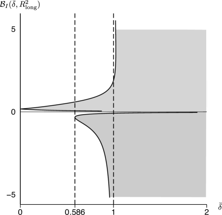
Figure 2: The cumulative identified set for the example of figure 1. Here we see that for large values of $\bar{\delta}$ the identified set includes every value in $\mathbb{R}$ except a small interval around 0. The set includes 0 for $\bar{\delta}\geq 32$, the explain away breakdown point. But the sign change breakdown point occurs much earlier, at $\delta=0.586$. Moreover, note that the identified set at $\bar{\delta}=1$ is $(-\infty,-0.0855]\cup[0.0432,1.8947]$. At $\bar{\delta}=1.05$ it is $(-\infty,-0.0798]\cup[0.0415,\infty)$.

We conclude this section with one additional useful feature of interval relaxations.

Proposition 1.

Suppose $r$ is an interval relaxation. Then

$$\mathcal{B}_{I}(r)=\{b\in\mathbb{R}:r^{\text{bf},=}(b)\leq r\}.$$

Proposition 1 shows that knowledge of the exact value breakdown point can be used to characterize identified sets, when $r$ is an interval relaxation. This is a kind of duality result, which shows that there is a one to one mapping between the identified set and the exact value breakdown point, so long as $r$ is an interval relaxation.

3 Setup and Identification Analysis

In this section we review the main identification results in Oster (2019), including her breakdown analysis. Importantly, we provide one new result in this section: We show that the set of possible biases due to omitted variables given in her Proposition 2 is sharp, up to a minor technical caveat. Consequently, that set can be correctly interpreted as the identified set for the bias. Her proof of Proposition 2 only showed that this set contained the true bias; it did not prove sharpness. This sharpness result is important because it shows that breakdown analysis based on this set is not unnecessarily conservative.

3.1 Regressions of Interest

Let $Y$ be an outcome variable, $X$ a treatment variable, $W_{1}$ a vector of observed covariates, and $W_{2}$ a vector of unobserved covariates. The following assumption ensures that the OLS estimands we will consider are well defined.

Assumption A3.

$\operatorname*{var}(Y,X,W_{1},W_{2})$ is finite. $\operatorname*{var}(X,W_{1},W_{2})$ and $\operatorname*{var}(Y,X,W_{1})$ are positive definite.

A1 allows $Y$ to be perfectly collinear with $(X,W_{1},W_{2})$, but not with $(X,W_{1})$. Collinearity of $Y$ with $(X,W_{1})$ would violate A3 below.

Consider three OLS regressions:

1. The short regression of

   $$Y\text{ on }(1,X).$$

   Let $\beta_{\text{short}}$ denote the corresponding population regression coefficient on $X$. Let $R_{\text{short}}^{2}$ denote the corresponding R-squared.

2. The medium regression of

   $$Y\text{ on }(1,X,W_{1}).$$

   Let $\beta_{\text{med}}$ denote the corresponding population regression coefficient on $X$. Let $R_{\text{med}}^{2}$ denote the corresponding R-squared. Let $\gamma_{1,\text{med}}$ denote the coefficients on $W_{1}$.

3. The long regression of

   $$Y\text{ on }(1,X,W_{1},W_{2}).$$

   Let $\beta_{\text{long}}$ denote the corresponding population regression coefficient on $X$. Let $R_{\text{long}}^{2}$ denote the corresponding R-squared. Note $R_{\text{long}}^{2}\in[R_{\text{med}}^{2},1]$. Let $(\gamma_{1,\text{long}},\gamma_{2,\text{long}})$ denote the coefficients on $(W_{1},W_{2})$.

Suppose $\beta_{\text{long}}$ is the parameter of interest. In particular, we can write the long regression as

$$Y=\beta_{\text{long}}X+\gamma_{1,\text{long}}^{\prime}W_{1}+\gamma_{2,\text{long}}^{\prime}W_{2}+Y^{\perp X,W}$$ (1)

where $Y^{\perp X,W}$ is defined to be the OLS residual plus the intercept term, and hence is uncorrelated with each component of $(X,W_{1},W_{2})$ by construction. The identification problem is that $W_{2}$ is not observed. Instead, we only assume that the joint distribution of $(Y,X,W_{1})$ is known. This allows us to point identify $\beta_{\text{short}}$ and $\beta_{\text{med}}$. These coefficients usually do not equal $\beta_{\text{long}}$, however. The difference between $\beta_{\text{long}}$ and either $\beta_{\text{short}}$ or $\beta_{\text{med}}$ is omitted variable bias. We next consider assumptions that will help us bound the magnitude of this omitted variable bias.

3.2 Comparing Selection on Observables and on Unobservables

Following the analysis of Altonji et al. (2005, pages 175–176), Oster (2019) recommends that we measure the magnitude of selection on unobservables via the parameter

$$\delta=\frac{\operatorname*{cov}(X,\gamma_{2,\text{long}}^{\prime}W_{2})}{\operatorname*{var}(\gamma_{2,\text{long}}^{\prime}W_{2})}\Bigg{/}\frac{\operatorname*{cov}(X,\gamma_{1,\text{long}}^{\prime}W_{1})}{\operatorname*{var}(\gamma_{1,\text{long}}^{\prime}W_{1})}.$$

To allow for cases where the denominator is zero, our formal analysis uses the following assumption.

Assumption A6.

There is a known $\delta\in\mathbb{R}$ such that

$$\delta\cdot\frac{\operatorname*{cov}(X,\gamma_{1,\text{long}}^{\prime}W_{1})}{\operatorname*{var}(\gamma_{1,\text{long}}^{\prime}W_{1})}=\frac{\operatorname*{cov}(X,\gamma_{2,\text{long}}^{\prime}W_{2})}{\operatorname*{var}(\gamma_{2,\text{long}}^{\prime}W_{2})}.$$ (2)

The following assumption, combined with A1, ensures that we are not dividing by zero in equation (2).

Assumption A9.

$\gamma_{1,\text{long}}\neq 0$ and $\gamma_{2,\text{long}}\neq 0$.

The parameter $\delta$ depends on two terms:

1. (“Selection on unobservables”) Regress $X$ on $(1,\gamma_{2,\text{long}}^{\prime}W_{2})$ and get the coefficient on the index $\gamma_{2,\text{long}}^{\prime}W_{2}$.

2. (“Selection on observables”) Regress $X$ on $(1,\gamma_{1,\text{long}}^{\prime}W_{1})$ and get the coefficient on the index $\gamma_{1,\text{long}}^{\prime}W_{1}$.

$\delta$ is the ratio of these two regression coefficients. $\delta$ is not known from the data since it depends on $W_{2}$, which is not observed, and $(\gamma_{1,\text{long}},\gamma_{2,\text{long}})$ which are also unknown. Instead, we will study what can be said about $\beta_{\text{long}}$ under assumptions on $\delta$. Several papers propose alternative sensitivity parameters, including Cinelli and Hazlett (2020) and Diegert et al. (2022). In this paper we instead use the same sensitivity parameter $\delta$ as Oster (2019), since our focus here is to study the implications of using different kinds of breakdown points. See Oster (2019), Cinelli and Hazlett (2020, section 6.3), and Diegert et al. (2022, appendix A.1) for further discussion of the interpretation of $\delta$.

Baseline covariates

$\delta$ is defined to calibrate the magnitude of selection on unobservables by using the observed covariates $W_{1}$. Typically we will have additional covariates $W_{0}$ which we want to include in the analysis, but not use for calibration. Denote these baseline controls by $W_{0}$. To incorporate these covariates, replace $(X,W_{1},W_{2})$ with $(X^{\perp W_{0}},W_{1}^{\perp W_{0}},W_{2}^{\perp W_{0}})$ throughout the entire analysis. See section 3.3 of Diegert et al. (2022) for a justification of this approach and further discussion. For simplicity, we omit $W_{0}$ throughout our theoretical analysis.

3.3 Identification of $\beta_{\text{long}}$

In this section we state a version of the main and most general identification result in Oster (2019). That paper also analyzes several special cases which we do not discuss for brevity. The main substantive assumption is the following.

Assumption A12 (Exogenous controls).

$\operatorname*{cov}(W_{1},W_{2})=0$.

A4 requires that all of the observed covariates are uncorrelated with the omitted variables. Appendix A.1 in Oster (2019) briefly discusses one approach to relaxing A4; see Appendix A of Diegert et al. (2022) for a detailed discussion of this approach. Diegert et al. (2022) also develop an alternative approach to sensitivity analysis that does not rely on A4. In this paper we maintain A4 throughout because our main focus is to study different notions of breakdown. For simplicity, from here on we assume $W_{2}$ is a scalar. All of our results can be generalized to vector $W_{2}$ using the arguments in appendix B of Diegert et al. (2022). We also maintain the following normalization.

Assumption A15 (Normalization).

$\operatorname*{var}(W_{2})=1$.

To state the main result, it is also useful to consider the regression of $X$ on $(1,W_{1})$. Let $\pi_{1}$ denote the coefficient on $W_{1}$. Let $X^{\perp W_{1}}=X-\pi_{1}^{\prime}W_{1}$.

Theorem 2.

Suppose the joint distribution of $(Y,X,W_{1})$ is known. Suppose A1–A5 hold. Suppose $R_{\text{long}}^{2}\in(R_{\text{med}}^{2},1]$ is known. Then the identified set for $\beta_{\text{long}}$ is

$$\mathcal{B}_{I}(\delta,R_{\text{long}}^{2})=\{b\in\mathbb{R}:f(\beta_{\text{med}}-b,\delta,R_{\text{long}}^{2})=0\}\setminus\mathcal{B}_{\text{A3fail}}$$

where

$$\mathcal{B}_{\text{A3fail}}=\{b\in\mathbb{R}:\gamma_{1,\text{med}}+(\beta_{\text{med}}-b)\pi_{1}=0\}$$

and $f(B,\delta,R_{\text{long}}^{2})=f_{0}(B)+\delta\cdot f_{1}(B,R_{\text{long}}^{2})$ with

$$f_{0}(B) =-B\operatorname*{var}(X^{\perp W_{1}})\left(\operatorname*{var}(\gamma_{1,\text{med}}^{\prime}W_{1})+2B\operatorname*{cov}(X,\gamma_{1,\text{med}}^{\prime}W_{1})+B^{2}\operatorname*{var}(\pi_{1}^{\prime}W_{1})\right)$$

$$f_{1}(B,R_{\text{long}}^{2}) =(R_{\text{long}}^{2}-R_{\text{med}}^{2})\operatorname*{var}(Y)\operatorname*{cov}(X,\gamma_{1,\text{med}}^{\prime}W_{1})+B(R_{\text{long}}^{2}-R_{\text{med}}^{2})\operatorname*{var}(Y)\operatorname*{var}(\pi_{1}^{\prime}W_{1})$$

$$\qquad+B^{2}\operatorname*{var}(X^{\perp W_{1}})\operatorname*{cov}(X,\gamma_{1,\text{med}}^{\prime}W_{1})+B^{3}\operatorname*{var}(X^{\perp W_{1}})\operatorname*{var}(\pi_{1}^{\prime}W_{1}).$$

Theorem 2 is a version of Oster’s (2019) Proposition 2. Most importantly, Oster’s Proposition 2 did not prove sharpness. Instead, that result only showed that $\{b\in\mathbb{R}:f(\beta_{\text{med}}-b,\delta,R_{\text{long}}^{2})=0\}$ is an outer set that contains the true parameter. Our Theorem 2 shows that this set is in fact essentially sharp and therefore can correctly be interpreted as the identified set. As we discuss below, this sharpness is important to ensure that breakdown analysis is not unnecessarily conservative. The only caveat is that the set $\mathcal{B}_{\text{A3fail}}$ must be subtracted to obtain sharpness. This set will typically be empty, however. This is a minor technical point so we discuss it at the end of this subsection.

There are several other minor differences between our Theorem 2 and Oster’s (2019) Proposition 2. We do not impose the normalization that $\operatorname*{var}(W_{1})$ is diagonal. Oster’s exogenous controls assumption is stated as $\operatorname*{cov}(W_{1},\gamma_{2,\text{long}}^{\prime}W_{2})=0$, which is equivalent to our A4 given that we are assuming for simplicity $W_{2}$ is scalar throughout the analysis, and since $\gamma_{2,\text{long}}\neq 0$ by A3.

As Oster (2019) discusses, the set

$$\{b\in\mathbb{R}:f(\beta_{\text{med}}-b,\delta,R_{\text{long}}^{2})=0\}$$

is the set of solutions to a cubic equation. Hence the identified set $\mathcal{B}_{I}(\delta,R_{\text{long}}^{2})$ has at most three elements. Figure 1 shows an example of this set, as a function of $\delta$.

Theorem 2 assumed $R_{\text{long}}^{2}>R_{\text{med}}^{2}$. The following result explains why: When $R_{\text{long}}^{2}=R_{\text{med}}^{2}$ the omitted variable bias is zero.

Proposition 2.

Suppose assumption A1 holds. Suppose $R_{\text{long}}^{2}=R_{\text{med}}^{2}$. Then $\beta_{\text{long}}=\beta_{\text{med}}$.

Finally, the analysis simplifies to the baseline case when $\delta=0$.

Corollary 1.

Suppose A1–A5 hold. Suppose $\delta=0$ and $\gamma_{1,\text{med}}\neq 0$. Then $\beta_{\text{long}}=\beta_{\text{med}}$.

The set $\mathcal{B}_{\text{A3fail}}$

Here we explain how to interpret $\mathcal{B}_{\text{A3fail}}$ and how to characterize when it is empty. By Lemma 1 in Appendix B,

$$\gamma_{1,\text{long}}=\gamma_{1,\text{med}}+(\beta_{\text{med}}-\beta_{\text{long}})\pi_{1}.$$ (3)

So $\mathcal{B}_{\text{A3fail}}$ is the set of $\beta_{\text{long}}$ values which would imply $\gamma_{1,\text{long}}=0$, which violates A3; recall that $\delta$ is not defined when A3 fails. This explains why such values must be removed. Next, notice that $\mathcal{B}_{\text{A3fail}}$ is nonempty if and only if there exists a $C\in\mathbb{R}$ such that $\gamma_{1,\text{med}}=C\pi_{1}$. That is, if and only if $\pi_{1}$ and $\gamma_{1,\text{med}}$ are proportional to each other. When $W_{1}$ is a vector, as is usually the case in empirical practice, this proportionality condition will typically not hold, and hence $\mathcal{B}_{\text{A3fail}}$ will be empty. When $W_{1}$ is a scalar, however, $\pi_{1}$ and $\gamma_{1,\text{med}}$ are scalars and hence are always proportional. In this case, the singleton $\mathcal{B}_{\text{A3fail}}=\{\beta_{\text{med}}+\gamma_{1,\text{med}}/\pi_{1}\}$ is not in the identified set. While the appearance of the set $\mathcal{B}_{\text{A3fail}}$ in Theorem 2 is mostly technical, it is nonetheless important, for example, when proving that the identified set is a singleton under the stronger assumptions in Proposition 4 below.

3.4 Oster’s Breakdown Analysis

Thus far we have characterized the identified set for $\beta_{\text{long}}$ when $\delta$ and $R_{\text{long}}^{2}$ are known. Next we consider breakdown analysis. In this section we review the main breakdown point result in Oster (2019). In section 4, we then apply our general analysis in section 2 to better understand the behavior of Oster’s breakdown analysis.

Let $\beta_{\text{hypo}}\in\mathbb{R}$. Define the exact value breakdown point

$$\delta^{\text{bp},=}(\beta_{\text{hypo}},R_{\text{long}}^{2})=\inf\{|\delta|:\delta\in\mathbb{R},\beta_{\text{hypo}}\in\mathcal{B}_{I}(\delta,R_{\text{long}}^{2})\}.$$

This is the smallest magnitude of the sensitivity parameter $\delta$ that is compatible with $\beta_{\text{long}}=\beta_{\text{hypo}}$. That is, for all $\delta$ with $|\delta|<\delta^{\text{bp},=}(\beta_{\text{hypo}},R_{\text{long}}^{2})$, we know that $\beta_{\text{hypo}}$ is not in the identified set $\mathcal{B}_{I}(\delta,R_{\text{long}}^{2})$. The next result gives a closed form solution for this value.

Theorem 3.

Suppose the joint distribution of $(Y,X,W_{1})$ is known. Suppose A1–A5 hold. Suppose $R_{\text{long}}^{2}\in(R_{\text{med}}^{2},1]$ is known. Suppose $\beta_{\text{long}}=\beta_{\text{hypo}}$ for a known $\beta_{\text{hypo}}\in\mathbb{R}\setminus\mathcal{B}_{\text{A3fail}}$. Suppose $\beta_{\text{short}}\neq\beta_{\text{med}}$. Then $\delta$ is point identified and equals

$$\frac{-f_{0}(\beta_{\text{med}}-\beta_{\text{hypo}})}{f_{1}(\beta_{\text{med}}-\beta_{\text{hypo}},R_{\text{long}}^{2})}.$$

Consequently, $\delta^{\text{bp},=}(\beta_{\text{hypo}},R_{\text{long}}^{2})$ equals its absolute value.

Theorem 3 is very similar to Oster’s Proposition 3, with only minor differences. As Oster remarked, this result shows that, even though knowledge of $\delta$ does not point identify $\beta_{\text{long}}$, knowledge of $\beta_{\text{long}}$ does point identify $\delta$. Figure 1 explains why: Fixing $\delta$ is equivalent to placing a vertical line on the plot. This vertical line may intersect the displayed curve up to three times, since $\mathcal{B}_{I}(\delta,R_{\text{long}}^{2})$ can have up to three elements. Fixing the value $\beta_{\text{long}}$ to be equal to some known $\beta_{\text{hypo}}$, however, is equivalent to placing a horizontal line on the plot. This line can only intersect the displayed curve once. The absolute value of the horizontal coordinate at this intersection is precisely $\delta^{\text{bp},=}(\beta_{\text{hypo}},R_{\text{long}}^{2})$.

Setting $\beta_{\text{hypo}}=0$, we get the explain away breakdown point

$$\delta^{\text{bp},\text{exact}}(R_{\text{long}}^{2})\equiv\delta^{\text{bp},=}(0,R_{\text{long}}^{2})=\frac{|f_{0}(\beta_{\text{med}})|}{|f_{1}(\beta_{\text{med}},R_{\text{long}}^{2})|}.$$

Its signed value, $-f_{0}(\beta_{\text{med}})/f_{1}(\beta_{\text{med}},R_{\text{long}}^{2})$, is often called Oster’s delta. Estimates of this value are commonly reported as a measure of the robustness of the baseline model $(\delta=0)$ to the presence of omitted variables. However, Oster’s $\delta$ is a deviation from the baseline model, not a relaxation (following definition 1). Therefore, as discussed in section 2, the explain away and sign change breakdown points are generally not equal. We compare these two breakdown points in the next section.

4 Measuring the Robustness of $\text{sign}(\beta_{\text{long}})$ to Omitted Variables

In this section we analyze the robustness of conclusions about the sign of $\beta_{\text{long}}$ to the presence of omitted variables. In section 4.1 we first show that the sign change breakdown point for $\delta$ can never be larger than 1. This is a concern since $\delta=1$ is often considered the cutoff for robustness, and therefore this result implies that conclusions about the sign of $\beta_{\text{long}}$ are always non-robust. In section 4.2 we propose a simple modification to Oster’s analysis that allows the sign change breakdown point to be larger than 1.

4.1 The Sign Change Breakdown Point for $\delta$

Oster’s delta answers the following question:

• Suppose we knew the exact value of $R_{\text{long}}^{2}$. What is the smallest value of $\delta$ that is required for the data to be consistent with $\beta_{\text{long}}=0$?

We call this the explain away breakdown point. Researchers may also be interested in answering the following question:

• Suppose we knew the exact value of $R_{\text{long}}^{2}$. What is the smallest value of $\delta$ such that $\beta_{\text{long}}$ has a different sign from $\beta_{\text{med}}$?

We call this the sign change breakdown point. Because Oster (2019) considers deviations from the baseline model rather than relaxations, Oster’s delta does not answer this question. In fact, as we next show, the sign change breakdown point is typically much smaller than the explain away breakdown point.

To formalize this claim, let

$$\delta^{\text{bp},\text{sign}}(R_{\text{long}}^{2})=\begin{cases}\delta^{\text{bp},>}(R_{\text{long}}^{2})&\text{if $\beta_{\text{med}}>0$}\\ \delta^{\text{bp},<}(R_{\text{long}}^{2})&\text{if $\beta_{\text{med}}<0$}\end{cases}$$

where

$$\delta^{\text{bp},>}(R_{\text{long}}^{2}) =\inf\{|\delta|:\delta\in\mathbb{R},b\leq 0\text{ for some }b\in\mathcal{B}_{I}(\delta,R_{\text{long}}^{2})\}$$

$$\delta^{\text{bp},<}(R_{\text{long}}^{2}) =\inf\{|\delta|:\delta\in\mathbb{R},b\geq 0\text{ for some }b\in\mathcal{B}_{I}(\delta,R_{\text{long}}^{2})\}.$$

We now state our main theoretical result.

Theorem 4.

Suppose A1–A5 hold. Suppose $\beta_{\text{short}}\neq\beta_{\text{med}}$. Then for any $R_{\text{long}}^{2}\in(R_{\text{med}}^{2},1]$,

$$\delta^{\text{bp},\text{sign}}(R_{\text{long}}^{2})\leq 1.$$

Here we assume $\beta_{\text{short}}\neq\beta_{\text{med}}$ for simplicity only. Theorem 4 shows that, in Oster’s sensitivity analysis, the sign change breakdown point can never be larger than one. In practice, researchers typically consider the value $\delta=1$ to be the cutoff for determining the robustness of a result. That is, they interpret values of $\delta$ greater than 1 as robust and values less than 1 as sensitive. Based on this criterion, Theorem 4 therefore shows that the sign of the parameter of interest is never robust (assuming we require $\delta$ strictly larger than 1 to conclude that the result is robust). In contrast, the explain away breakdown point $\delta^{\text{bp},\text{exact}}(R_{\text{long}}^{2})$ is often substantially larger than one. We illustrate this difference empirically in section 6.

Figure 1 illustrates the intuition for this result: The graph $\{(\delta,b)\in\mathbb{R}^{2}:f(\beta_{\text{med}}-b,\delta,R_{\text{long}}^{2})=0\}$ has an asymptote at $\delta=1$. Consequently, values of $\delta$ close to one—but not equal to one—yield identified sets that contain arbitrarily large or arbitrarily small values. Hence for $\delta$ values near one we cannot point identify the sign of $\beta_{\text{long}}$. Since we are only considering a deviation, however, much larger values of $\delta$ may be needed before the graph crosses the horizontal axis $b=0$ exactly. This explains why the explain away breakdown point can often be much larger than the sign change breakdown point for this model.

4.2 Incorporating Magnitude Restrictions on the Omitted Variable Bias

We have just shown that the sign change breakdown point for $\delta$ can never be larger than one. This negative result can be overturned by adding additional identifying assumptions. We consider the following particularly simple assumption.

Assumption A18.

$|\beta_{\text{long}}-\beta_{\text{med}}|\leq M$ for some known $M\geq 0$.

A6 says that the magnitude of the omitted variable bias is no larger than $M$. We discuss the choice of $M$ below. This assumption can be viewed as formalizing Oster’s (2019) statement that researchers may be “willing to assume that the bias is fairly small” (page 194).

Corollary 2.

Suppose the joint distribution of $(Y,X,W_{1})$ is known. Suppose A1–A6 hold. Suppose $R_{\text{long}}^{2}\in(R_{\text{med}}^{2},1]$ is known. Suppose $\delta\in\mathbb{R}$ is known. Then the identified set for $\beta_{\text{long}}$ is

$$\mathcal{B}_{I}(\delta,R_{\text{long}}^{2},M)=\mathcal{B}_{I}(\delta,R_{\text{long}}^{2})\cap[\beta_{\text{med}}-M,\beta_{\text{med}}+M].$$

Let $\delta^{\text{bp},\text{sign}}(R_{\text{long}}^{2},M)$ denote the corresponding sign change breakdown point. For $0\leq M<\infty$, it is now possible for $\delta^{\text{bp},\text{sign}}(R_{\text{long}}^{2},M)>1$. We illustrate this empirically in section 6.

Thus far we have followed Oster (2019) by considering deviations from the baseline model—our identification results (Theorem 2 and Corollary 2) have assumed the exact value of $\delta$ is known. Consequently, when we also make the magnitude restriction A6 the model can be falsified. To avoid this, we next convert the analysis to a relaxation of the baseline model. Specifically, we make the following assumption.

Assumption A21.

There is a known constant $\bar{\delta}\geq 0$ such that $|\delta|\leq\bar{\delta}$.

This leads to the following identification result.

Corollary 3.

Suppose the joint distribution of $(Y,X,W_{1})$ is known. Suppose A1–A5 and A7 hold. Suppose $R_{\text{long}}^{2}\in(R_{\text{med}}^{2},1]$ is known. Then the identified set for $\beta_{\text{long}}$ is

$$\mathcal{B}_{I}(\bar{\delta},R_{\text{long}}^{2})=\bigcup_{|\delta|\leq\bar{\delta}}\mathcal{B}_{I}(\delta,R_{\text{long}}^{2}).$$

Suppose A6 also holds. Then the identified set for $\beta_{\text{long}}$ is

$$\mathcal{B}_{I}(\bar{\delta},R_{\text{long}}^{2},M)=\bigcup_{|\delta|\leq\bar{\delta}}\mathcal{B}_{I}(\delta,R_{\text{long}}^{2},M).$$

This corollary simply notes that we take the union of the identified sets from Theorem 2 over all allowed values of the sensitivity parameter $\delta$ with magnitude less than $\bar{\delta}$ to obtain the identified set.

Choosing $M$

$M$ is the largest difference between the known $\beta_{\text{med}}$ and the unknown $\beta_{\text{long}}$. The choice of this parameter should therefore reflect the researcher’s beliefs about this difference. If $M=0$ then $\beta_{\text{long}}=\beta_{\text{med}}$ is point identified regardless of the magnitude of selection on unobservables. Therefore $M$ should not be chosen too small. If $M$ is large, the magnitude restriction will not bind and therefore will not affect the sensitivity analysis. We recommend that researchers consider a range of magnitude restrictions, as we illustrate empirically in section 6. One simple approach is to choose $M$ to be multiples of $\beta_{\text{med}}$. That is, let $M=p\cdot\beta_{\text{med}}$ for $p\geq 0$. For this choice, A6 is equivalent to

$$\beta_{\text{long}}\in[(1-p)\beta_{\text{med}},(1+p)\beta_{\text{med}}].$$

Every element of this set has the same sign if and only if $p\leq 1$. For this reason, since we are interested in robustness to sign changes, $p$ should be chosen strictly larger than 1. For example, in section 6 we consider $p=2$, $3$, and $10$.

5 The Sensitivity of Bias Adjusted Estimands

Thus far we have focused on breakdown analysis. Researchers also commonly compute point estimands that adjust for omitted variable bias. See our survey in section 7 for examples from the empirical economics literature. When the sensitivity parameter is a deviation, as in Oster’s (2019) analysis, we show that this kind of bias adjustment can be extremely sensitive to perturbations in the choice of sensitivity parameter. We also discuss several additional concerns about common practice when using Oster’s (2019) results to do bias adjustment. We then make a recommendation which addresses these concerns. We conclude by discussing a common mistake some researchers make when computing explain away breakdown points, along with a remark about the “bounding set” defined in Oster (2019).

5.1 Adding Assumptions to Point Identify $\beta_{\text{long}}$

In this subsection we describe the most common approach by which empirical researchers use Oster’s (2019) results to compute bias adjusted estimands. Theorem 2 generally does not point identify $\beta_{\text{long}}$, which means there is not a unique way to compute a bias adjusted estimand. However, as Oster shows, the identified set in Theorem 2 simplifies to a singleton under two additional assumptions. The first assumption is $\delta=1$. The second assumption is the following, which is equivalent to Oster’s assumption 2 (page 192).

Assumption A24.

There is a constant $C\in\mathbb{R}$ such that $\gamma_{1,\text{long}}=C\cdot\pi_{1}$.

Recall that $\pi_{1}$ denotes the coefficient on $W_{1}$ in the regression of $X$ on $(1,W_{1})$. A8 holds immediately when $W_{1}$ is a scalar, but otherwise is a restriction. In fact, the following result implies that A8 is refutable and confirmable (as defined in Breusch 1986) under exogenous controls. Hence the data alone tells us whether it holds.

Proposition 3.

Suppose A1 and A4 hold. Then A8 holds if and only if there is a constant $C_{\text{med}}\in\mathbb{R}$ such that $\gamma_{1,\text{med}}=C_{\text{med}}\cdot\pi_{1}$.

For vector $W_{1}$, Oster (2019) said A8 “is very unlikely to hold except in pathological cases” (page 192). Proposition 3 shows that researchers do not need to guess about this assumption—it can be directly tested in the data. Such a hypothesis test can be constructed using standard minimum distance methods, by comparing $\widehat{\gamma}_{1,\text{med}}$ with multiples of $\widehat{\pi}_{1}$; we omit a full development for brevity.

Under these two additional assumptions, $\delta=1$ and A8, we can now show that $\beta_{\text{long}}$ is point identified.

Proposition 4.

Suppose the joint distribution of $(Y,X,W_{1})$ is known. Suppose A1, A3, A4, A5, and A8 hold. Suppose A2 holds with $\delta=1$. Suppose $R_{\text{long}}^{2}\in(R_{\text{med}}^{2},1]$ is known. Suppose $\beta_{\text{short}}\neq\beta_{\text{med}}$. Then $\beta_{\text{long}}$ is point identified and

$$\beta_{\text{long}}=\beta_{\text{med}}+(\beta_{\text{med}}-\beta_{\text{short}})\frac{R_{\text{long}}^{2}-R_{\text{med}}^{2}}{R_{\text{med}}^{2}-R_{\text{short}}^{2}}.$$ (4)

This result is a version of Oster’s Proposition 1. Oster’s (2019) proof is slightly incomplete, however, since it only shows that the value in equation (4) is consistent with the data. It does not show that this is the only value that is consistent with the data. Our proof of Proposition 4 shows this last step. In this proof we show how the result follows directly from our Theorem 2: The cubic function $f(\beta_{\text{med}}-b,\delta,R_{\text{long}}^{2})$ is quadratic with two solutions when $\delta=1$ and one of the two solutions is eliminated by subtracting $\mathcal{B}_{\text{A3fail}}$. The remaining solution is equation (4). Finally, in this result we assume $\beta_{\text{short}}\neq\beta_{\text{med}}$ to ensure that $R_{\text{short}}^{2}\neq R_{\text{med}}^{2}$ and hence that the right hand side of (4) is well defined.

5.2 The Sensitivity of the Equation (4) Adjustment

Many papers use equation (4) to produce bias adjusted estimates. There are three issues with this approach. First, it is only valid when A8 holds. Fortunately, as we showed in Proposition 3, we can use the data to directly test this assumption. Second, as discussed in Diegert et al. (2022), equation (4) relies on the exogenous controls assumption A4.

Third, equation (4) is only valid when $\delta=1$. Theorem 2 characterizes the feasible values of $\beta_{\text{long}}$ when $\delta\neq 1$. In our earlier analysis, we saw that when $\delta$ is very close to one, but not equal to one, the identified set for $\beta_{\text{long}}$ will contain values with arbitrarily large magnitudes; note that this is true even when A8 holds. Consequently, bias adjustments based on equation (4) are arbitrarily sensitive to perturbations of $\delta$. Therefore, for researchers to view bias adjusted estimands with $\delta=1$ as useful robustness check, they must believe that $\delta$ exactly equals 1, and is not merely close to 1. We illustrate this sensitivity in table 6.3 in our empirical application.

Importantly, these large values are equally as valid as the smallest element of the identified set. That is, under the assumptions of Theorem 2, there is no justification for ruling out the possibility that the true bias is one of these large values. The only way to rule out these values is to make additional assumptions. One such assumption is the magnitude restriction A6 that we discuss in section 4.2. The identified set $\mathcal{B}_{I}(\bar{\delta},R_{\text{long}}^{2},M)$ that we describe in that section formally incorporates this magnitude restriction. However, even if we impose this magnitude restriction, the cumulative identified set $\mathcal{B}_{I}(\bar{\delta},R_{\text{long}}^{2},M)$ can still easily contain both positive and negative elements even with $\bar{\delta}=1$. This can be seen by superimposing the bound implied by A6 onto figure 2 or 3. Consequently, even with a magnitude restriction, bias adjustments based on equation (4) will be sensitive to changes in $\delta$.

5.3 Recommendations

We have shown that bias corrections based on equation (4) are either not valid because A8 fails, or are highly dependent on $\delta$ being exactly 1, and therefore are extremely sensitive to perturbations of $\delta$. A simple alternative is to present a plot of the identified set $\mathcal{B}_{I}(\bar{\delta},R_{\text{long}}^{2})$ for $\beta_{\text{long}}$ as a function of $\bar{\delta}\geq 0$. We described this set in section 4.2. This set describes the values of $\beta_{\text{long}}$ consistent with any amount of selection on unobservables $\delta$ with magnitude less than $\bar{\delta}$. Hence, unlike a single point estimand for $\delta=1$, it shows how the feasible values of $\beta_{\text{long}}$ vary for a range of $\delta$ values. Moreover, since it is based on Theorem 2, this set does not require assumption A8 to be valid. See figure 2 for an example, and figure 3 for the simpler convex hull of this set. Note that all these recommendations continue to rely on A4, which is not testable. Researchers who wish to relax this assumption should use an alternative method, like Diegert et al. (2022).

5.4 A Common Mistake when Computing Explain Away Breakdown Points

As pointed out in Diegert et al. (2022), several papers compute the explain away breakdown point $\delta^{\text{bp},\text{exact}}(R_{\text{long}}^{2})$ incorrectly (the correct value is given by Theorem 3). We conclude this section by describing the source of this mistake. It can be avoided by using software based on the correct results, such as Oster’s package psacalc or our package regsensitivity in Stata.

Proposition 4 shows how to point identify $\beta_{\text{long}}$ if $\delta=1$, $R_{\text{long}}^{2}$ is known, and A8 is assumed. The identification result in Theorem 2 is strictly more general since it allows for any value of $\delta$ and does not use A8. Because this general theorem holds for any $\delta$, it should be used for breakdown analysis, as we did earlier. However, on page 193 Oster (2019) states the following equation:

$$\beta_{\text{long}}\approx\beta_{\text{med}}+\delta(\beta_{\text{med}}-\beta_{\text{short}})\frac{R_{\text{long}}^{2}-R_{\text{med}}^{2}}{R_{\text{med}}^{2}-R_{\text{short}}^{2}}$$ (5)

where $\delta$ is no longer necessarily equal to one. We are not aware of any formal results which justify this equation—Oster (2019) does not provide any and does not explain the nature of the approximation $\approx$ in this equation. To the contrary, as we explained earlier, Theorem 2 implies that $\beta_{\text{long}}$ can be arbitrarily far from its value at $\delta=1$ even for $\delta$ values arbitrarily close to 1. Moreover, even at $\delta=1$, $\beta_{\text{long}}$ is not necessarily point identified when A8 is not assumed. Consequently, equation (5) should not be used to perform sensitivity analysis (except when $\delta$ is exactly equal to 1 and under the other conditions of Proposition 4).

Several researchers, however, have apparently used equation (5) to compute breakdown points. This includes Satyanath et al. (2017, JPE) and Bazzi et al. (2020, ECMA). Specifically, they fix $R_{\text{long}}^{2}$ and solve

$$\beta_{\text{med}}+\delta(\beta_{\text{med}}-\beta_{\text{short}})\frac{R_{\text{long}}^{2}-R_{\text{med}}^{2}}{R_{\text{med}}^{2}-R_{\text{short}}^{2}}=0$$

for $\delta$. This solution does not equal the explain away breakdown point $\delta^{\text{bp},\text{exact}}(R_{\text{long}}^{2})$. Note that this is true even if A8 holds—Proposition 4 is only about the case $\delta=1$ and does not describe the bias when $\delta\neq 1$.

Equation (5) also explains why some papers do not report the magnitude of their computed $\delta^{\text{bp},\text{exact}}$ when it is negative. For example, Satyanath et al. (2017) report “[$<$ 0]” in their Table A.27 results rather than providing the exact magnitude of negative estimates. In the table footnote, they say

“The entry [$<$0] indicates that the respective Altonji et al. ratio is negative… suggesting a downward bias for our OLS estimates due to unobservables”. (online appendix page 44)

If equation (5) were correct for all $\delta$, then the sign of the omitted variable bias would be determined by the sign of $\delta$ and $\beta_{\text{med}}-\beta_{\text{short}}$. So it is incorrect to conclude that the true bias $\beta_{\text{med}}-\beta_{\text{long}}$ is negative whenever this breakdown point is negative. Regardless, this line of reasoning is all based on equation (5) which, as we explained above, generally does not hold except when $\delta$ is exactly equal to 1 and under the other conditions of Proposition 4.

5.5 Remark on Oster’s “Bounding Set”

Based on the discussion on pages 194–196, Oster (2019) defines

$$\beta^{*}(\delta,R_{\text{long}}^{2})=\operatorname*{argmin}_{b\in\mathcal{B}_{I}(\delta,R_{\text{long}}^{2})}\;|\beta_{\text{med}}-b|.$$

Using this, she defines the set $[\beta_{\text{med}},\beta^{*}(\delta,R_{\text{long}}^{2})]$ (or the reverse if $\beta_{\text{med}}$ is the larger value). She calls this a “bounding set” on page 196, but elsewhere calls it the “identified set” (for example, see her Table 3). The discussion on page 196 suggests that this interval should be interpreted as the identified set for $\beta_{\text{long}}$ under the assumption that $0\leq\delta\leq 1$. As we have shown, this is not the correct interpretation. This follows because Oster’s model is a deviation, not a relaxation, and hence the identified set $\mathcal{B}_{I}(\delta,R_{\text{long}}^{2})$ for a known $\delta$ is not monotonic in $\delta$. Note that this is generally true even if we impose the magnitude constraint A6. The correct identified set under the assumption that $0\leq\delta\leq 1$ is given by $\mathcal{B}_{I}(\bar{\delta},R_{\text{long}}^{2})$ from Corollary 3 with $\bar{\delta}=1$. Figure 2 plots an example of this set; figure 3 plots its convex hull. We recommend that researchers present this set, rather than the “bounding set” described above.

Finally, note that some authors (for example, Mian and Sufi 2014, ECMA, online appendix page 2) define $\beta^{*}(\delta,R_{\text{long}}^{2})$ as the value from equation (4), from Oster’s Proposition 1. This is equivalent to the definition above when $\delta=1$ and A8 holds, but otherwise they are different. Regardless, this approach also leads to an interval that does not have the correct interpretation as an identified set.

6 Empirical Application: Social Capital and the Rise of the Nazi Party

Social capital is typically viewed as a good which leads to good outcomes for countries. For example, de Tocqueville (1835) famously argued that social capital was a key reason why American democracy thrived. More recently, Putnam (2000) argued that the decline in social capital threatened American democracy. Satyanath et al. (2017, JPE) argue the converse: “Our paper is the first to show—on the basis of detailed cross-sectional data—that social capital can undermine and help to destroy a democratic system” (page 482). They specifically look at the rise of the Nazi Party (the National Socialist German Worker’s Party [NSDAP]) in 1933. Overall, they argue that “vibrant networks of clubs and associations facilitated the rise of the Nazi Party” (page 520). In contrast, earlier literature blamed the rise of the Nazis

“on a ‘civic non-age’ of low social capital (Stern 1972) and Nazi entry on rootless, isolated individuals in a modernized society (Shirer 1960; Arendt 1973)” (page 520)

They also qualify their results by arguing that

“where government was more stable, the link between association density and Nazi Party entry was weaker” and hence “the effects of social capital depend crucially on the political and institutional context”

Their paper has a variety of analyses. We focus on their main results, which use a selection on observables identification strategy paired with linear models.

6.1 Data

We first describe the data. See section 3 of Satyanath et al. (2017) for further details. The units of analysis are towns/cities in Germany. The sample size is $n=229$. The outcome variable $Y$ is a measure of how many people in that city joined the Nazi party. The treatment variable $X$ is a measure of social capital. Thus they are interested in whether there was a causal effect of having a large amount of social capital within a city on the rate at which new members joined the Nazi party within that city. Satyanath et al. (2017) use three different measures of social capital. All three are based on “association density,” the number of social clubs and associations per 1,000 city inhabitants. There are 22,127 different associations in the sample. The authors classify these into three types:

1. Military associations: Stahlhelm (“steel helmet”), veterans associations.

2. Civic associations (have “a clearly nonmilitaristic/nationalist outlook”): Animal breeding, music, chess, hiking, women’s, citizens’, and homeland (heimat) clubs, and some others (predominantly civic clubs, many with an artistic or creative pursuit such as gardening, theatre, or photography).

3. Other: Sports, choirs, gymnastics, shooting, students/fraternities, lodges, youth, oldfellows, hunting, gentlemen, corps.

$X$ is then defined to be the density of all associations, of civic associations only, or of military associations only.

Next consider the control variables. Recall from section 3.2 that we distinguish between two kinds of observed control variables: Those which we use for comparison in the sensitivity analysis ($W_{1}$) and those which we do not ($W_{0}$). The baseline controls $W_{0}$ are population, share Catholic, and share blue-collar, all defined for 1925. The comparison covariates $W_{1}$ are

• Socioeconomic controls: share of Jews (1925), share unemployed (1933), welfare recipients per 1000 (1933), war participants per 1000 (1933), social insurance pensioners per 1000 (1933), log average income tax payment (1933), log average property tax payment (1933).

• Political controls: Hitler speeches per 1000 (1932), average DNVP votes 1920–1928, average DVP votes 1920–1928, average SPD votes 1920–1928, average KPD votes 1920–1928.

In their appendix G, Satyanath et al. (2017) also consider using the variables in $W_{0}$ for calibration; we omit this analysis for brevity. In their baseline analysis, they also include state fixed effects as covariates. They do not include these in their sensitivity analysis, however.

6.2 Baseline Model Results

[caption = Baseline results for Satyanath et al. (2017). , remarkNote = These estimates replicate part of table 3 in Satyanath et al. (2017): Column (1) replicates Panel A, columns (4)–(6). Column (3) replicates Panel B, columns (4)–(6). Panel C, column (2) replicates Panel B, column (3). Panels A and B, column (2) were not presented in table 3 of Satyanath et al. (2017). ***, **, *: statistically significant at 1%, 5%, 10%.] p0.20¿ *3¿p0.10 Dependent Variable: Nazi Party Entry, 1925–January 1933
(1) (2) (3)
A. Treatment = All Associations
0.160*** 0.170*** 0.087*
(0.053) (0.050) (0.047)
B. Treatment = Civic Associations
0.430*** 0.439*** 0.284***
(0.130) (0.120) (0.100)
C. Treatment = Military Associations
0.829*** 0.855*** 0.613*
(0.264) (0.263) (0.330)
Controls:
  Baseline X X X
  Socioeconomic X X
  Political X X
  State Fixed Effects X

Table 6.2 shows the baseline regression results. Column (1) shows the estimated coefficient $\widehat{\beta}_{\text{short}}$ on $X$ from OLS of $Y$ on $(1,X,W_{0})$, along with its standard error. Panels A–C show this coefficient for the three different definitions of the treatment variable $X$. First consider Panel A. This is their most broad definition of treatment, accounting for all kinds of associations. We see that the estimated coefficient is positive and statistically significantly different from zero at the 1% level. Thus, adjusting for the baseline controls $W_{0}$, cities with more social capital, as measured by density of all associations, had higher rates of new membership in the Nazi party.

Does this result reflect a broad causal effect of social capital on entry into the Nazi party? One counter-argument is that it may merely reflect the effect of a specific kind of social capital—membership in military specific associations. Indeed, in Panel C we see that, when restricting attention to military associations, the estimated coefficient is again positive and statistically significantly different from zero at the 1% level. However, suppose we restrict attention to civic associations, which are defined to be non-militaristic and non-nationalistic. Panel B shows these estimates. There we continue to see a positive point estimate that is statistically significantly different from zero at the 1% level. This finding suggests that the effect is not driven solely by military specific social capital.

Are these results driven by omitted variable bias? The authors consider a variety of alternative methods to answer this question. We focus on just two: (i) Using additional controls and (ii) Using formal econometric methods for sensitivity analysis. Column (2) of Table 6.2 includes the additional controls $W_{1}$ in the regressions. Specifically, it shows the estimated coefficient $\widehat{\beta}_{\text{med}}$ on $X$ from OLS of $Y$ on $(1,X,W_{0},W_{1})$, along with its standard error. Panels A–C again show this coefficient for the three different versions of treatment. We again see that all of the point estimates are positive and statistically significantly different from zero at the 1% level. Column (3) adds state fixed effects. The point estimates are smaller but still positive and statistically significantly different from zero at the 10% level. On page 500 the authors explain that this drop in precision arises from the fact that some of the historical policies which drove variation in association density often varied at the state level.

6.3 Assessing Selection on Observables with Sensitivity Analysis

Interpreting the results of Table 6.2 as causal effects of social capital requires a selection on observables assumption: Association density is randomly assigned conditional on the included covariates. In their section 6, Satyanath et al. (2017) provide a wide variety of robustness checks to support this causal interpretation. This includes an application of Oster (2019) in subsection 4.D, with details provided in their appendix G. In this section we present the findings from this sensitivity analysis, as informed by the analysis in our paper.

Breakdown Analysis

[talltblr]rowsep=0pt [ caption = Robustness of Satyanath et al. (2017) Results to Omitted Variables., remarkNote = For all specifications, the $W_{0}$ includes the baseline controls while the calibration covariates $W_{1}$ includes the socioeconomic and political controls. See the text for a complete list of these variables. For comparison with column (1), in column (2) we also report the sign of the estimate obtained from Theorem 3. Column (7) reports the estimated breakdown point proposed in the alternative analysis of Diegert et al. (2022)., ]c — c *6¿p0.065 — c Oster (2019) This Paper DMP (2022)
$R_{\text{long}}^{2}$ $\widehat{\delta}^{\text{bp},\text{exact}}(R_{\text{long}}^{2})$ $\widehat{\delta}^{\text{bp},\text{sign}}(R_{\text{long}}^{2},M)$ with $M$ equal to $\widehat{\bar{r}}_{X}^{\text{bp}}$
Reported Correct $+\infty$ $10\widehat{\beta}_{\text{med}}$ $3\widehat{\beta}_{\text{med}}$ $2\widehat{\beta}_{\text{med}}$
(1) (2) (3) (4) (5) (6) (7)
All $1$ $<0$ $-32.0$ 0.586 0.586 0.586 0.676 0.538
$1.3\widehat{R}_{\text{med}}^{2}$ - $-331.5$ 0.953 0.954 1.476 2.829
Civic $1$ $<0$ 0.98 0.736 0.736 0.736 0.745 0.648
$1.3\widehat{R}_{\text{med}}^{2}$ - 9.78 0.994 1.036 1.806 2.986
Military $1$ $<0$ 1.42 0.899 0.899 0.909 0.977 0.761
$1.3\widehat{R}_{\text{med}}^{2}$ - 10.65 0.993 1.035 1.821 3.058

Table 6.3 shows the main breakdown results. This table replicates and extends the bottom half of Panel B in Table A.27 of appendix G in Satyanath et al. (2017). That part of Panel B only uses $W_{1}$ for calibration. The top half uses both $W_{0}$ and $W_{1}$ for calibration; we omit this analysis for brevity. The three rows of Table 6.3 correspond to the three different versions of treatment. All of the cell entries are different kinds of breakdown points.

First consider columns (1) and (2). These show estimates of Oster’s explain away breakdown point. We present estimates for two different choices of $R_{\text{long}}^{2}$, either 1 or Oster’s rule of thumb $1.3\widehat{R}_{\text{med}}^{2}$. Column (1) shows the values reported by Satyanath et al. (2017). As described in section 5.4, these values are incorrect. Column (2) reports the correct values. If we judged robustness by comparing the magnitude of these values of the explain away breakdown point to 1, then all of the results would be deemed robust except one, civic associations with $R_{\text{long}}^{2}=1$, which gives an explain away breakdown point of 0.98.

However, as we have discussed in this paper, the explain away breakdown point can be very different from the sign change breakdown point. Columns (3)–(6) show estimated sign change breakdown points, for four increasingly restrictive choices of the constraint on the magnitude $M$ of OVB: $+\infty$ (no constraint), $10\widehat{\beta}_{\text{med}}$, $3\widehat{\beta}_{\text{med}}$, and $2\widehat{\beta}_{\text{med}}$. First consider column (3), which does not impose any magnitude restriction. As implied by Theorem 4, we see that all of the point estimates are bounded above by 1. Nonetheless, as explained in section 3.3 of Diegert et al. (2022), 1 should not necessarily be viewed as a universal cutoff for robustness. Indeed, for the rule of thumb choice of $R_{\text{long}}^{2}$, all three sign change breakdown points are very close to 1, their largest possible value. This suggests that findings of positive coefficients in Table 6.2 are substantially robust to the presence of omitted variables. This finding is somewhat muted, however, if we consider different choices of $R_{\text{long}}^{2}$. Specifically, for the largest possible choice, $R_{\text{long}}^{2}=1$, the sign change breakdown points shrink a fair amount. Still, the sign change breakdown point when examining civic associations is 0.736, which is reasonably far from zero.

As explained in section 4.2, we can obtain sign change breakdown points larger than 1 if we impose additional restrictions. Columns (4)–(6) show the estimated sign change breakdown points when we restrict the magnitude of OVB to be below $M$. For the relatively unrestrictive value of $M=10\widehat{\beta}_{\text{med}}$, this additional restriction does not change the sign change breakdown points much. However, it is enough such that two of the breakdown points are now slightly above 1. For the more restrictive values $M=3\widehat{\beta}_{\text{med}}$ and $M=2\widehat{\beta}_{\text{med}}$, the breakdown points are now all substantially about 1 for the rule of thumb choice $R_{\text{long}}^{2}=1.3\widehat{R}_{\text{med}}^{2}$. For $R_{\text{long}}^{2}=1$, however, the magnitude restrictions do not affect the values of the sign change breakdown points very much.

The last column of Table 6.3 shows the estimated breakdown point $\widehat{\bar{r}}_{X}^{\text{bp}}$ developed in Diegert et al. (2022). This point does not require the exogenous controls assumption A4. It is based on an interval relaxation, and hence it is a sign change breakdown point. It also does not require a choice of $R_{\text{long}}^{2}$. Like the breakdown points based on Oster (2019), larger values represent larger magnitudes of selection on unobservables relative to selection on observables. Like the sign change breakdown point in column (3), it is also bounded above by 1. In column (7) we see that this alternative sensitivity analysis produces a similar pattern of robustness as the sign change breakdown points in Oster’s model: The results for military associations are most robust, followed by civic associations, and then followed by the overall measure (recall that the overall measure includes associations which are neither military nor civic).

Selection Bias Adjustments

Satyanath et al. (2017) did not present selection bias adjusted estimands; as we document in section 7, it is rare for empirical researchers to present both breakdown analysis and bias adjustments. To illustrate the results of section 5, here we also use bias adjustments to analyze the sensitivity of the results in Satyanath et al. (2017).

Table 6.3 summarizes our bias adjustment results. For brevity, here we focus on just the “all associations” treatment variable and the specification in column (2) of table 6.2, and we only consider $R_{\text{long}}^{2}=1$. Our findings are similar for the other treatment variables, specifications, and $R_{\text{long}}^{2}$ values. For simplicity we also do not present confidence sets for these point estimates. Panel A represents current empirical practice. The first row shows the baseline estimate. The second row shows the selection bias adjusted estimate obtained from Oster’s Proposition 1 (our Proposition 4), which assumes $\delta=1$ and requires A8. Based on this estimate, the researcher would conclude that selection bias only works in their favor—it has the same sign as their baseline estimate and indeed is even larger.

However, now consider the results in Panel B. If we maintain $\delta=1$ but drop A8, then there are now two values of the coefficient that are consistent with the assumptions and the data, and one of them is negative. Hence even this minor change from current practice overturns the robustness finding based on Oster’s Proposition 1 alone. Now, a researcher may claim that the value $-0.0855$ is close to zero, and perhaps is not statistically significantly different from zero, in which case one may argue that Oster’s Proposition 2 with $\delta=1$ still weakly supports a positive effect. So next we consider perturbing $\delta$ a slight amount: If we set $\delta=0.99$ then the identified set now includes a large negative value, $-18.66$. Likewise, if we set $\delta=1.01$ then the identified set includes a large positive value, $15.64$. Thus we see that the magnitude of the bias adjustment is very sensitive to the specific choice of $\delta$. Finally, the last two rows of Panel B show the identified sets when we replace the assumption that $\delta$ is known exactly with the assumption that we only have a bound $\bar{\delta}$ on its magnitude (A7). Here we see that for $\bar{\delta}=1$, almost every negative value is consistent with the data and the assumptions, and many positive values are as well, including some bigger and smaller than the baseline estimate. If we increase this bound slightly to $\bar{\delta}=1.05$ then arbitrarily large values of the coefficient are possible too. In Table 6.3 we have considered just a few values of $\delta$ or $\bar{\delta}$. Figure 2 shows the identified sets from Oster’s proposition 2 for a large range of $\delta$’s. Figure 3 shows the convex hull of the identified sets from our Corollary 3 for a large range of $\bar{\delta}$’s. Note that the magnitude constraint A6 can be imposed by simply superimposing horizontal lines at the largest and smallest feasible values on this plot.

[caption = The Sensitivity of Bias Adjustments. , remarkNote = All estimates are for the “all associations” specification from Satyanath et al. (2017). All sensitivity methods use $R_{\text{long}}^{2}=1$ and require exogenous controls, A4.] p0.38¿ *1¿p0.13 *1¿p0.31 Method Assumptions $\beta_{\text{long}}$ Values
A. Current Practice
Baseline Estimate $\delta=0$ 0.170
Oster’s Prop 1 (our Prop 4) $\delta=1$, A8 0.532
B. Sensitivity to $\delta$ Assumptions
Oster’s Prop 2 (our Thm 2), $\widehat{\mathcal{B}}_{I}(\delta,R_{\text{long}}^{2})$ $\delta=1$ $\{-0.0855,\,1.8947\}$
Oster’s Prop 2, $\widehat{\mathcal{B}}_{I}(\delta,R_{\text{long}}^{2})$ $\delta=0.99$ $\{-18.66,\,-0.0868,\,1.736\}$
Oster’s Prop 2, $\widehat{\mathcal{B}}_{I}(\delta,R_{\text{long}}^{2})$ $\delta=1.01$ $\{-0.0843,\,2.133,\,15.64\}$
Corollary 3, $\widehat{\mathcal{B}}_{I}(\bar{\delta},R_{\text{long}}^{2})$ $|\delta|\leq\bar{\delta}=1$ $(-\infty,-0.0855]\cup[0.0432,1.8947]$
Corollary 3, $\widehat{\mathcal{B}}_{I}(\bar{\delta},R_{\text{long}}^{2})$ $|\delta|\leq\bar{\delta}=1.05$ $(-\infty,-0.0798]\cup[0.0415,\infty)$

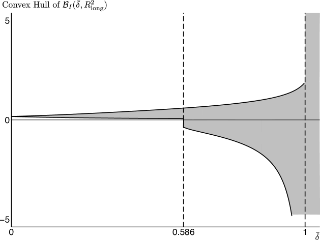
Figure 3: The convex hull of the estimated identified set for $\beta_{\text{long}}$ under the assumption that $R_{\text{long}}^{2}$ is known and $|\delta|\leq\bar{\delta}$. Here we consider the “all associations” specification from Satyanath et al. (2017) and set $R_{\text{long}}^{2}=1$. This plot is the convex hull of the plot in figure 2.

To better understand the estimates in Tables 6.3 and 6.3, we next plot estimated identified sets $\widehat{\mathcal{B}}_{I}(\delta,R_{\text{long}}^{2})$ as a function of $\delta$ for the 3 choices of treatment variables and 2 choices of $R_{\text{long}}^{2}$. Figure 4 shows these plots. These plots show several of the features we discussed earlier in the paper. For example, at $\delta=0$, the identified set is the singleton containing $\widehat{\beta}_{\text{med}}$. This is displayed as the horizontal intercept. The vertical intercept, in contrast, is the explain away breakdown point, as reported in column (2) of Table 6.3. Only two of these intercepts are visible given the range of the plots, however.

As $\delta$ varies, the identified set can contain either 1, 2, or 3 elements. For example, in the top left graph, there are two feasible values of $\beta_{\text{long}}$ at $\delta=1$. We can also see the vertical asymptote at $\delta=1$, which implies that for $\delta$’s very close to 1, the identified set will contain either very large positive values, very large negative values, or both. This explains why the identified set under the restriction $|\delta|\leq\bar{\delta}$ is bounded and finite for $\bar{\delta}<1$ but unbounded for $\bar{\delta}>1$. It also explains why the bias adjustments in Table 6.3 are so sensitive to the exact choice of $\delta$.

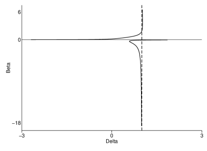
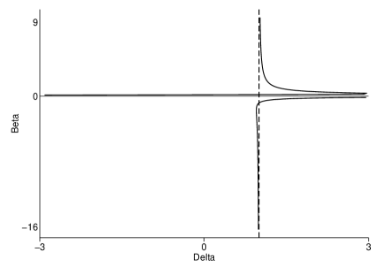
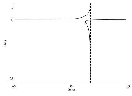
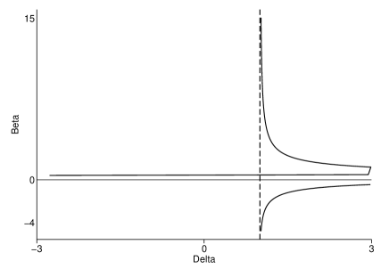
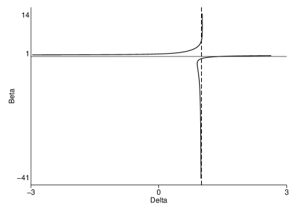
Figure 4: Estimated identified sets $\widehat{\mathcal{B}}_{I}(\delta,R_{\text{long}}^{2})$ for assessing the robustness of Satyanath et al. (2017) results to omitted variables. Left column: $R_{\text{long}}^{2}=1$. Right column: $R_{\text{long}}^{2}=1.3\widehat{R}_{\text{med}}^{2}$. Top row: Treatment variable includes all associations. Middle row: Treatment variable includes civic associations only. Bottom row: Treatment variable includes military associations only.

6.4 Empirical Conclusions

Overall, Table 6.3 shows just how different the explain away and sign change breakdown points can be in practice. By only examining the explain away breakdown point, Satyanath et al. (2017) conclude that

“selection on unobservables would have to be substantially stronger than selection on observables for our main result to be overturned.” (online appendix page 44)

The language “for our main result to be overturned”, however, suggests that they are also interested in the robustness of their point estimates to sign changes. Indeed, if the true coefficient $\beta_{\text{long}}$ was negative then higher social capital would lead to a decrease in Nazi party membership, which would support the opposite of their conclusion that social capital supported the Nazi party and therefore helped to undermine an existing democracy.

When examining the relative robustness of their results for the three versions of the treatment variable, a second concern arises. Based on the explain away breakdown point, they say:

“Note also that for the logic of our argument, the coefficient for military associations is not the most important—what matters is that the civic clubs and associations have an important effect on Nazi Party entry. This is never in doubt in the Altonji-Elder-Taber/Oster exercise.” (online appendix page 44)

When examining the sign change breakdown points, however, we see that the coefficient for military associations is the most robust, among the three versions of treatment. The coefficient for civic clubs and associations, in contrast, is not so obviously robust to omitted variables. Thus the sign change breakdown points suggest a more tentative conclusion about robustness than the definitive one drawn by the authors.

Moreover, our analysis of selection bias adjustments in Table 6.3 illustrates how sensitive these kinds of adjustments can be to the choice of $\delta$ in practice. The bounds presented in Figure 3 provide a modified sensitivity analysis method that accurately represents the impact of omitted variables on the range of possible coefficient values.

7 A Survey of Regression Sensitivity Analysis in Practice

To understand how empirical researchers are using Oster (2019) in practice, we performed a survey of the empirical economics literature. We constructed the sample by looking at all papers published in the three year period from 2019 to 2021, which cite Oster (2019), and which were published in either AER, JPE, QJE, REStud, or ECMA. This gives 35 papers. 1 of these is an econometric theory which cited Oster (2019) as a related method only, and so we drop it from the sample. 3 of these papers used the methods in Oster (2019), but only in working paper drafts, not in the final published version. We drop these 3 from the sample as well. This leaves 31 papers remaining. These papers are listed in Appendix C.

This sample size is similar to the survey of Blandhol et al. (2022), who found 112 papers that use 2SLS in the same five journals, over the 19 year span from January 2000 to October 2018. In fact, since we are only looking at 3 years of data, Oster’s (2019) method is more popular than 2SLS, on average, since 112 papers over 19 years is only about 18 papers every three years. This is perhaps not surprising since Oster’s results can be applied to regressions based on many different identification strategies, including unconfoundedness, instrumental variables, and difference-in-differences (see section 4 of Diegert et al. 2022 for a related discussion).

There are three different ways in which researchers apply the results of Oster (2019):

1. Report the explain away breakdown point.

2. Report a bias adjusted estimand.

3. Informally discuss coefficient stability and cite Oster (2019) as justification.

Table 7 summarizes the distribution of these three methods across the 31 papers in our dataset. We see that roughly 75% of the papers use and report the results of one of the two formal sensitivity analysis methods. Among these, roughly half only report breakdown points, and about half report bias adjusted estimands. Only a few papers do both. The remaining roughly 25% of papers only informally discuss coefficient stability, and refer to Oster (2019) in their discussion. Some of those discussions suggest that they may have used one of the formal methods, but if so they did not report the findings. Although it is not the focus of this paper (cf. Diegert et al. 2022), none of the 31 papers discuss the validity of the exogenous controls assumption A4.

[talltblr]rowsep=0pt [ caption = How Empirical Researchers Use Oster (2019). , remarkNote = Sample contains 31 papers published in AER, QJE, JPE, ECMA, or REStud between 2019–2021 and which use Oster (2019)., ] p0.48¿ — *1¿p0.20 *1¿p0.15 Proportion Count
Total 100% 31
1. Compute Explain Away Breakdown Points 42% 13
And vary $R_{\text{long}}^{2}$ 15% (conditional) 2
2. Compute Bias Adjusted Estimates 39% 12
And vary $\delta$ 17% (conditional) 2
And vary $R_{\text{long}}^{2}$ 42% (conditional) 5
3. Discuss Informally Only 26% 8
Both 1 and 2 6% 2

Consider the papers that report the explain away breakdown point. Very few also vary $R_{\text{long}}^{2}$. Most use either $1.3\widehat{R}_{\text{med}}^{2}$ or 1. One paper also used $2\widehat{R}_{\text{med}}^{2}$. One paper presented the function $\widehat{\delta}^{\text{bp},\text{exact}}(R_{\text{long}}^{2})$ as $R_{\text{long}}^{2}$ varied from $\widehat{R}_{\text{med}}^{2}$ to 1. When discussing their results, researchers used a variety of phrases to describe their estimates of $\delta^{\text{bp},\text{exact}}(R_{\text{long}}^{2})$: It is the amount of selection on unobservables relative to observables needed…

• “to fully explain away the coefficient on the explanatory variable of interest” (Arbatli, Ashraf, Galor, and Klemp 2020, ECMA, page 747)

• “to make our core estimate go away” (Dippel and Heblich 2021, AER, page 491)

• “to drive the results observed” (Valencia Caicedo 2019, QJE, online appendix page 6)

• “for our results to be spuriously generated” (Grosfeld, Sakalli, and Zhuravskaya 2020, REStud, page 296)

• “to reverse the sign of the results” (Hoffman and Tadelis 2021, JPE, page 272)

to give a few examples from our survey. As we have shown in this paper, the last quote is incorrect, because the sign change and explain away breakdown points are not equivalent. The first quote correctly describes it as an explain away breakdown point. The other three quotes are more ambiguous, and the interpretation depends on what it means for an estimate to “go away,” or “to drive the results,” or for the “results to be spuriously generated.” If these statements refer to the sign of the main finding, rather than the conclusion that the effect is not exactly zero (but might be positive or negative), then these descriptions are incorrect. Our paper clarifies that empirical researchers must specify whether they are interested in robustness to sign changes, or merely to an exact zero.

Next consider the papers that report bias adjusted estimands. For any given specification, all of these papers report a scalar bias adjusted estimand. Most papers explicitly say that this is because they use Oster’s Proposition 1 (see our Prop. 4) and assume $\delta=1$. Others do not clearly explain which result they are using to obtain their bias correction. None of the papers that use Oster’s Proposition 1 discuss validity of assumption A8. Nine of the twelve papers use just the single value $\delta=1$. One paper considers $\delta=0.5$ only (and no other values), but also uses the incorrect equation (5) as described in section 5. Two of the papers consider multiple $\delta$ values, but one of them also uses the incorrect equation (5). The other paper uses a variation of Oster’s results, which we have not formally analyzed, although we conjecture that the concerns we raise in our paper will apply to that extension as well. About half of the papers only consider one value of $R_{\text{long}}^{2}$, always either $1.3\widehat{R}_{\text{med}}^{2}$ or 1. In the other half, four papers also consider the second value $2\widehat{R}_{\text{med}}^{2}$, while one paper considers up to 4 different values.

Overall, the results in our paper clarify and improve upon all three of the main ways in which empirical researchers use the methods of Oster (2019).

8 Conclusion: Best Practices for Regression Sensitivity Analysis

We conclude by providing several recommendations for best practices. Here we focus on Oster’s analysis, given its widespread adoption, but these recommendations often apply to other methods as well. Moreover, all of these recommendations are easy to implement using our companion Stata package regsensitivity.

1. Use sign change breakdown points to measure robustness

Throughout this paper we have emphasized the difference between the explain away and sign change breakdown points. Empirical researchers who are interested in the robustness of the sign of $\beta_{\text{long}}$ to omitted variables should use sign change breakdown points, either instead of or in addition to explain away breakdown points. For Oster’s (2019) model, we developed this sign change breakdown point in section 4.

2. Present identified sets for a range of sensitivity parameter values

We showed that bias adjusted estimands can be extremely sensitive to small perturbations of the sensitivity parameter. We therefore recommend that, rather than presenting a single bias corrected estimand, researchers plot sharp bounds on the parameter of interest for a wide range of the sensitivity parameters.

3. Do not rely on coefficient stability alone to assess the role of omitted variables

Oster’s (2019) Proposition 1 (our Prop. 4) is a key result that links omitted variable bias to coefficient stability. She remarks, however, that her analysis “make[s] clear the limits of coefficient stability: it is possible that the coefficient will be completely unchanged with the addition of controls but there may still be a large bias on the treatment effect” (page 188). She later concludes that her “core insight is to recognize that coefficient stability on its own is at best uninformative and at worst very misleading” (page 203). Her caveats are based primarily on two features of her analysis: (i) A8 could be violated (see the first sentence of page 195), in which case her Proposition 1 (our Prop. 4) no longer holds and (ii) Even when A8 holds, the magnitude of the bias in that proposition also depends on $R_{\text{long}}^{2}$.

Our analysis pushes her conclusion even further: We show that, even if the true value of $R_{\text{long}}^{2}$ was known, and even if A8 holds, then the bias adjustment in Oster’s Proposition 1 is extremely sensitive to the assumption that $\delta=1$. In particular, regardless of how close the short and medium regression coefficients are, the true bias can be arbitrarily large when $\delta$ is close but not equal to 1. Moreover, as Diegert et al. (2022) emphasize, Oster’s Proposition 1 also requires the exogenous controls assumption A4.

Overall, the econometric theory evidence to date does not support the conclusion that coefficient stability alone is informative about the magnitude of omitted variable bias. This does not, however, imply that tests of coefficient stability are uninformative more generally. For example, Chen and Pearl (2015) show how coefficient stability tests can be viewed as falsification tests for causal graphs with enough exclusion restrictions to yield several different sets of observed covariates that lead to conditionally independent treatment assignment. Future work in econometrics would be helpful to further clarify the exact nature and value of coefficient stability exercises. In lieu of this, we recommend using a formal regression sensitivity analysis method, like those discussed in this paper and the related literature.

4. Use a range of values for auxiliary sensitivity parameters

Several sensitivity analysis methods focus on a primary sensitivity parameter, like Oster’s $\delta$, but also require assumptions about an auxiliary sensitivity parameter, like $R_{\text{long}}^{2}$. As we saw in section 7, researchers commonly fix this auxiliary parameter to a single value. In section 6, however, we saw that empirical results can often be quite sensitive to the choice of these auxiliary sensitivity parameters. We therefore recommend exploring a range of values for these auxiliary sensitivity parameters.

5. Consider using a variety of methods for sensitivity analysis

There is now a large menu of options for researchers interested in performing a regression sensitivity analysis. These methods are typically not nested, and make different assumptions about the role of omitted variables. Consequently, it can be useful to use several different methods together. We illustrated this in section 6 where we also applied the analysis of Diegert et al. (2022) to address the exogenous controls assumption. In that empirical application we saw that the modifications to Oster’s breakdown analysis developed in section 4 generally leads to similar conclusions about the robustness of the empirical results as Diegert et al. (2022). When a variety of sensitivity analyses all point in the same direction, researchers can be more confident in the robustness of their results.

Appendix A Additional Empirical Applications

Beyond our empirical application in section 6, we also considered all six papers published in the American Economic Review from our section 7 survey which formally implemented the Oster (2019) method. Among these papers, three had complete, publicly available replication data and code. In this section, we apply our methods to the data from these three papers. For brevity we only present the results; see the original papers for a discussion of the full empirical context, analysis, and data. Two of the three papers only presented breakdown point estimates, while the third paper only presented bias adjustments.

1. Squicciarini (2020, AER)

In this paper, the author estimates explain away breakdown points for two different outcome variables, and reports them in table A.11 of the online appendix. Based on these estimates, the author concludes

“that selection on unobservables would have to be at least 4.1 times stronger than selection on observables to explain away the relationship between the [treatment variable] and the outcome variables, making it unlikely that unobserved factors are confounding the results.” (page 20)

In table A, we replicate and extend this analysis. Column (1) shows the explain away breakdown point estimates as reported and correctly computed by the original author. Column (2) shows the estimated sign change breakdown points. Consistent with our theorem 4, these are less than one. However, they are quite close to one. In columns (3)–(5) we add magnitude restrictions. Column (3) shows that even with a fairly loose magnitude restriction we are able to obtain sign change breakdown points above one. And, especially for the first outcome variable, we can substantially increase the breakdown point with further magnitude restrictions. Finally, column (6) shows estimated breakdown points based on the method in Diegert et al. (2022). Recall that these breakdown points account for sign changes, do not rely on magnitude restrictions, and cannot be larger than one without further restrictions. Their values are reasonably large, with one of them above 50% (0.5). That value of $\bar{r}_{X}$ can be interpreted as meaning that selection on observables is twice as large as selection on unobservables.

Overall, our analysis here shows that although the explain away breakdown points are substantially larger than the sign change breakdown points, if one uses the conventional cutoffs for robustness and imposes some magnitude restrictions on the OVB, the author’s conclusion that their results are robust to omitted variables continues to hold.

[talltblr]rowsep=0pt [ caption = Robustness of Squicciarini (2020) Results to Omitted Variables., remarkNote = See original paper for variables included in $W_{1}$. $R_{\text{long}}^{2}=1$ for all results in columns (1)–(5)., ]c — *1¿p0.145 *4¿p0.065 — c Oster (2019) This Paper DMP (2022)
$\widehat{\delta}^{\text{bp},\text{exact}}(R_{\text{long}}^{2})$ $\widehat{\delta}^{\text{bp},\text{sign}}(R_{\text{long}}^{2},M)$ with $M$ equal to $\widehat{\bar{r}}_{X}^{\text{bp}}$
$+\infty$ $10\widehat{\beta}_{\text{med}}$ $3\widehat{\beta}_{\text{med}}$ $2\widehat{\beta}_{\text{med}}$
Outcome variable (1) (2) (3) (4) (5) (6)
Share Ind. Workers 9.09500.99821.36833.44944.69860.4097
Machines 4.06990.99681.07441.83062.44600.5369

2. Dippel and Heblich (2021, AER)

In table 2 on page 491, the authors report estimates of the explain away breakdown point. On that page, they say

“To get a sense for potential selection on unobservables in the full and matched sample, we report Oster’s $\delta$ in the bottom of Table 2. Oster’s $\delta$ measures how large the bias from unobservables would have to be relative to bias from observable to imply a true value of $\beta=0$ in equation (1). In the full sample, $\delta$ is consistently around 0.5. In the matched sample by contrast, $\delta$ ranges between 1.7 and 1.9. This implies a strong sense of robustness in the matched sample, where selection on unobservables would have to be almost twice as strong as selection on observables to make our core estimate go away.” [emphasis added]

Our extended analysis, shown in table A, is qualitatively similar: The results appear robust for the matched sample but not the full sample. Specifically, first consider the full sample. Consider the first line, the core controls; the results are similar for the other two choices of controls. In column (1) we see that the estimated explain away breakdown point is 0.5170. This is also the sign change breakdown point, as shown in column (2). Given that this value is substantially less than 1, where the asymptote in the identified set appears, imposing magnitude constraints (columns (3)–(5)) does not affect the value of the sign change breakdown point. In the last column we see that the breakdown point of Diegert et al. (2022) is less than 50% (0.5). All of these results together suggest that the results for the full sample are not robust.

Next consider the matched sample. Consider the first line, the core controls; the results are similar for the other two choices of controls. Here we see the estimated explain away breakdown point is 1.7073. This is not the sign change breakdown point, however. In this case, the sign change breakdown point is exactly 1. Nonetheless, with even a loose magnitude constraint—assuming the OVB is bounded above by $10\widehat{\beta}_{\text{med}}$—the sign change and explain away breakdown points coincide exactly. Further magnitude restrictions are not helpful because these restrictions only matter insofar as they bring the sign change and explain away breakdown points closer together. Finally, applying the results of Diegert et al. (2022), the matched sample breakdown point is larger than 50% (0.5). Overall, these results suggest that the results for the matched sample are robust.

[talltblr]rowsep=0pt [ caption = Robustness of Dippel and Heblich (2021) Results to Omitted Variables., remarkNote = See original paper for variables included in each choice of $W_{1}$. $R_{\text{long}}^{2}=1$ for all results in columns (1)–(5)., ]c c — *1¿p0.145 *4¿p0.065 — c Oster (2019) This Paper DMP (2022)
$\widehat{\delta}^{\text{bp},\text{exact}}(R_{\text{long}}^{2})$ $\widehat{\delta}^{\text{bp},\text{sign}}(R_{\text{long}}^{2},M)$ with $M$ equal to $\widehat{\bar{r}}_{X}^{\text{bp}}$
$+\infty$ $10\widehat{\beta}_{\text{med}}$ $3\widehat{\beta}_{\text{med}}$ $2\widehat{\beta}_{\text{med}}$
Sample $W_{1}$ (1) (2) (3) (4) (5) (6)
Core controls 0.51700.51700.51700.51700.51700.1570
Full + other Vselect 0.5187 0.51870.51870.51870.51870.1556
All controls 0.5156 0.51560.51560.51560.51560.1533
Core controls 1.7073 1.00001.70731.70731.70730.5337
Matched + other Vselect 1.9654 1.00001.96541.96541.96540.5300
All controls 1.9554 1.00001.95541.95541.95540.5068

3. Gregg (2020, AER)

This paper uses Oster’s results in tables 3, 5, and 7 of the main paper. For brevity we only consider the results in table 3. The author considers three different outcome variables, and two choices of sample and calibration covariates $W_{1}$ for each outcome variable. Unlike the two papers we considered above, Gregg does not estimate breakdown points. Instead, they only present bias adjusted estimates. Specifically, following Oster’s (2019) recommendation and the defaults in the accompanying Stata package psacalc, panel B of table 3 of Gregg (2020) reports the single element of the estimated identified set obtained from Oster’s proposition 2 (our theorem 2) which is closest to $\widehat{\beta}_{\text{med}}$ (this is an estimate of the value $\beta^{*}(\delta,R_{\text{long}}^{2})$ defined in section 5.5). Using these estimates, Gregg provides the following analysis:

Some suggestive evidence on the nature of selection is provided by the Oster (2017) bound listed for each regression in panel B of Table 3. Here I report the estimate of the coefficient on corporation in the case where the selection on unobservables is equal to the selection on observables (when $\delta$ equals 1). The observables in this case are the province, industry, and year controls. These coefficients suggest some positive selection in revenue per worker, but possibly some negative selection in machine power per worker and TFP. Columns 4–6 introduce controls for the factory’s age, which makes little difference for the revenue per worker or power per worker regressions. However, factory age is highly correlated with TFP, since age proxies for survival. Furthermore, with the age control included, the estimated Oster bound indicates positive selection in the TFP regression, likely since selection on the newly included observable, factory age, was substantial.” (pages 414–415)

In this analysis Gregg uses Oster’s method to assess the direction of the selection bias, by comparing the bias adjusted estimates with the baseline estimates. Overall, Gregg concludes that there is positive selection bias, meaning that the baseline estimates are too large. In our analysis, we show that Gregg’s conclusion about the direction of selection bias no longer holds once we account for the sensitivity of the bias adjusted estimands obtained using Oster’s method.

To see this, we replicate and extend her estimates for each of the three outcome variables in table A. First consider panel I, for the $\log(\text{R}/\text{L})$ outcome variable. Consider specification 1. Gregg compared the element of the set $\{0.412,197\}$ that is closest to the baseline estimate 0.495 with that baseline estimate. This gives $0.412<0.495$, suggesting that the baseline estimate is too big. Similarly, in specification 2 we see that $0.331<0.451$, suggesting again that the baseline estimate is too big. There are two main concerns with this comparison, however. First, it ignores the other element of the estimated Proposition 2 identified set. For example, in specification 1 the baseline estimate $0.495$ is smaller than $197$, the other element of the estimated identified set. This comparison suggests that the baseline estimate is too small.

Now, as in our discussion of magnitude restrictions in section 4.2, one might be willing to eliminate this second element by imposing an additional assumption that restrictions the magnitude of the coefficient. This does not salvage the argument, however, because there is a second issue: In the fourth line of panel B we show the estimated cumulative identified set under the assumption that $|\delta|\leq 1$. This set is a union of two intervals. Even if we ignore the upper interval, this set is $[0.412,0.550]$. This set contains values that are smaller and larger than the baseline estimate of 0.495. Thus if we allow for $\delta$ to take any value so long as its magnitude is not larger than 1, rather than assuming that $\delta$ is exactly equal to 1, then we can no longer conclude anything about the direction of the selection bias. A similar analysis holds for the second specification, and the other two outcome variables.

[caption = The Sensitivity of Bias Adjustments in Gregg (2020). , remarkNote = All sensitivity methods use $R_{\text{long}}^{2}=1$. Panel I: Specification 1 corresponds to column (1) of Panel B in table 3 of Gregg (2020) while specification 2 corresponds to column (4). Panel II: Specification 1 corresponds to column (2) of Panel B in table 3 of Gregg (2020) while specification 2 corresponds to column (5). Panel III: Specification 1 corresponds to column (3) of Panel B in table 3 of Gregg (2020) while specification 2 corresponds to column (6).] p0.40¿ *1¿p0.15 *1¿p0.40 *1¿p0.40 $\beta_{\text{long}}$ Values
Method Assumptions Specification 1 Specification 2
I. Outcome variable: $\log(\text{R}/\text{L})$
A. Current Practice
   Baseline Estimate $\delta=0$ 0.495 0.451
   Oster’s Prop 1 (our Prop 4) $\delta=1$, A8 0.434 0.367
B. Sensitivity to $\delta$ Assumptions
   Oster’s Prop 2 (our Thm 2), $\widehat{\mathcal{B}}_{I}(\delta,R_{\text{long}}^{2})$ $\delta=1$ $\{0.412,197\}$ $\{0.331,152\}$
   Oster’s Prop 2, $\widehat{\mathcal{B}}_{I}(\delta,R_{\text{long}}^{2})$ $\delta=0.9999$ $\{0.412,210,3200\}$ $\{0.331,158,3817\}$
   Oster’s Prop 2, $\widehat{\mathcal{B}}_{I}(\delta,R_{\text{long}}^{2})$ $\delta=1.01$ $\{-99.8,0.411,67.1\}$ $\{-99.0,0.329,60.7\}$
   Corollary 3, $\widehat{\mathcal{B}}_{I}(\bar{\delta},R_{\text{long}}^{2})$ $|\delta|\leq\bar{\delta}=1$ $[0.412,0.550]\cup[197,\infty)$ $[0.331,0.526]\cup[152,\infty)$
   Corollary 3, $\widehat{\mathcal{B}}_{I}(\bar{\delta},R_{\text{long}}^{2})$ $|\delta|\leq\bar{\delta}=1.05$ $(-\infty,-39.2]\cup[0.407,0.553]\cup[33.8,\infty)$ $(-\infty,-37.9]\cup[0.323,0.529]\cup[31.4,\infty)$
II. Outcome variable: $\log(\text{HP}/\text{L})$
A. Current Practice
   Baseline Estimate $\delta=0$ 0.250 0.216
   Oster’s Prop 1 (our Prop 4) $\delta=1$, A8 0.804 0.782
B. Sensitivity to $\delta$ Assumptions
   Oster’s Prop 2 (our Thm 2), $\widehat{\mathcal{B}}_{I}(\delta,R_{\text{long}}^{2})$ $\delta=1$ $\{-25.8,0.9532\}$ $\{-39.5,0.9525\}$
   Oster’s Prop 2, $\widehat{\mathcal{B}}_{I}(\delta,R_{\text{long}}^{2})$ $\delta=0.99$ $\{-367,-27.4,0.9449\}$ $\{-393,-43.4,0.9439\}$
   Oster’s Prop 2, $\widehat{\mathcal{B}}_{I}(\delta,R_{\text{long}}^{2})$ $\delta=1.01$ $\{-99.8,0.411,67.1\}$ $\{-36.6,0.961,464\}$
   Corollary 3, $\widehat{\mathcal{B}}_{I}(\bar{\delta},R_{\text{long}}^{2})$ $|\delta|\leq\bar{\delta}=1$ $(-\infty,-25.8]\cup[-0.301,0.9532]$ $(-\infty,-39.4]\cup[-0.358,0.9525]$
   Corollary 3, $\widehat{\mathcal{B}}_{I}(\bar{\delta},R_{\text{long}}^{2})$ $|\delta|\leq\bar{\delta}=1.05$ $(-\infty,-21.0]\cup[-0.326,0.995]\cup[95.0,\infty)$ $(-\infty,-30.2]\cup[-0.383,0.996]\cup[111,\infty)$
III. Outcome variable: TFP
A. Current Practice
   Baseline Estimate $\delta=0$ 0.102 0.015
   Oster’s Prop 1 (our Prop 4) $\delta=1$, A8 0.132 -0.141
B. Sensitivity to $\delta$ Assumptions
   Oster’s Prop 2 (our Thm 2), $\widehat{\mathcal{B}}_{I}(\delta,R_{\text{long}}^{2})$ $\delta=1$ $\{-211,0.163\}$ $\{-0.876,24.3\}$
   Oster’s Prop 2, $\widehat{\mathcal{B}}_{I}(\delta,R_{\text{long}}^{2})$ $\delta=0.99999$ $\{-7090,-218,0.163\}$ $\{-0.876,24.3,22452\}$
   Oster’s Prop 2, $\widehat{\mathcal{B}}_{I}(\delta,R_{\text{long}}^{2})$ $\delta=1.01$ $\{-35.6,0.167,43.0\}$ $\{-35.9,-0.922,14.6\}$
   Corollary 3, $\widehat{\mathcal{B}}_{I}(\bar{\delta},R_{\text{long}}^{2})$ $|\delta|\leq\bar{\delta}=1$ $(-\infty,-212]\cup[0.079,0.163]$ $[-0.876,0.115]\cup[24.3,\infty)$
   Corollary 3, $\widehat{\mathcal{B}}_{I}(\bar{\delta},R_{\text{long}}^{2})$ $|\delta|\leq\bar{\delta}=1.05$ $(-\infty,-16.5]\cup[.079,0.168]\cup[18.0,\infty)$ $(-\infty,-11.0]\cup[-1.16,0.118]\cup[7.93,\infty)$

Appendix B Proofs

Let $\mathbb{L}(A\mid B)$ denote the linear projection of the scalar random variable $A$ on the random column vector $B$, defined as $\mathbb{L}(A\mid B)=\mathbb{E}(AB^{\prime})\mathbb{E}(BB^{\prime})^{-1}B$.

Section 2

Proof of Theorem 1.

Let $b<\beta_{\text{baseline}}$. Define the following sets of relaxations:

$$R =\{r\geq 0:(-\infty,b]\cap\mathcal{B}_{I}(r)\neq\emptyset\}$$

$$\widetilde{R} =\{r\geq 0:\{b\}\cap\mathcal{B}_{I}(r)\neq\emptyset\}.$$

By definition, $r^{\text{bp},>}(b)=\inf(R)$ and $r^{\text{bp},=}(b)=\inf(\widetilde{R})$. By construction, $\widetilde{R}\subseteq R$ and $r^{\text{bp},>}(b)\leq r^{\text{bp},=}(b)$.

Next, we want to show that $R\subseteq\widetilde{R}$ and therefore $r^{\text{bp},>}(b)=r^{\text{bp},=}(b)$. Since $\mathcal{B}_{I}(r)$ is an interval relaxation, $(-\infty,b]\cap\mathcal{B}_{I}(r)$ is an intersection of two intervals, and is thus an interval. Since $\beta_{\text{baseline}}\in\mathcal{B}_{I}(0)$, $\beta_{\text{baseline}}>b$, and by $r$ being an interval relaxation, the set $\mathcal{B}_{I}(r)$ is an interval containing values greater than $b$ for any $r$. Therefore, if $(-\infty,b]\cap\mathcal{B}_{I}(r)\neq\emptyset$, then $b\in\mathcal{B}_{I}(r)$ and therefore $\{b\}\cap\mathcal{B}_{I}(r)\neq\emptyset$. This implies $R\subseteq\widetilde{R}$, and that $r^{\text{bp},>}(b)=r^{\text{bp},=}(b)$.

A similar proof holds when $b>\beta_{\text{baseline}}$. ∎

Proof of Proposition 1.

We have

$$\{b\in\mathbb{R}:r^{\text{bp},=}(b)\leq r\} =\{b\in\mathbb{R}:\inf\{\tilde{r}\geq 0:b\in\mathcal{B}_{I}(\tilde{r})\}\leq r\}$$

$$=\{b\in\mathbb{R}:b\in\mathcal{B}_{I}(r)\}$$

$$=\mathcal{B}_{I}(r).$$

The first equality follows by the definition of $r^{\text{bp},=}(b)$. The second equality follows from the monotonicity of $\mathcal{B}_{I}(\tilde{r})$ in $\tilde{r}$. Specifically, the statement

$$\inf\{\tilde{r}\geq 0:b\in\mathcal{B}_{I}(\tilde{r})\}\leq r$$

means there exists an $\tilde{r}\leq r$ such that $b\in\mathcal{B}_{I}(\tilde{r})$. So monotonicity implies that $b\in\mathcal{B}_{I}(r)$ since $r\geq\tilde{r}$. This is an equivalence because $b\in\mathcal{B}_{I}(r)$ implies there exists $\tilde{r}\leq r$ (namely, $\tilde{r}=r$) such that $b\in\mathcal{B}_{I}(\tilde{r})$. ∎

Section 3

It is useful to also consider the linear projection of $X$ onto $(1,W_{1},W_{2})$:

$$X=\pi_{1,\text{long}}^{\prime}W_{1}+\pi_{2,\text{long}}W_{2}+X^{\perp W}.$$ (6)

Then

$$\pi_{1} \equiv\operatorname*{var}(W_{1})^{-1}\operatorname*{cov}(W_{1},X)$$

$$=\operatorname*{var}(W_{1})^{-1}\operatorname*{cov}(W_{1},W_{1}^{\prime}\pi_{1,\text{long}}+W_{2}\pi_{2,\text{long}}+X^{\perp W})$$

$$=\operatorname*{var}(W_{1})^{-1}(\operatorname*{var}(W_{1})\pi_{1,\text{long}}+\operatorname*{cov}(W_{1},W_{2})\pi_{2,\text{long}}+\operatorname*{cov}(W_{1},X^{\perp W}))$$

$$=\pi_{1,\text{long}}.$$

The third line follows by the exogenous controls assumption A4. Similarly, if we let $\pi_{2}$ denote the coefficient on $W_{2}$ from the linear projection of $X$ onto $(1,W_{2})$ then $\pi_{2}=\pi_{2,\text{long}}$. Given these results, we use $(\pi_{1},\pi_{2})$ to represent the common values of the regression coefficients throughout the proofs.

We denote the omitted variable bias by $B=\beta_{\text{med}}-\beta_{\text{long}}$. We begin by showing the following identities that we’ll use throughout our proofs.

Lemma 1 (Regression Algebra).

Suppose A1, A4, and A5 hold. Then the following hold:

$$\gamma_{1,\text{long}} =\gamma_{1,\text{med}}+B\pi_{1}$$ (7)

$$\pi_{2}\gamma_{2,\text{long}} =B\operatorname*{var}(X^{\perp W_{1}})$$ (8)

$$\operatorname*{cov}(X,\gamma_{1,\text{med}}^{\prime}W_{1}) =(\beta_{\text{short}}-\beta_{\text{med}})\operatorname*{var}(X)$$ (9)

$$(R^{2}_{\text{med}}-R^{2}_{\text{short}})\operatorname*{var}(Y) =\operatorname*{var}(\gamma_{1,\text{med}}^{\prime}W_{1})-\operatorname*{var}(X)(\beta_{\text{short}}-\beta_{\text{med}})^{2}.$$ (10)

Proof of Lemma 1.

Proof of (7)

We have that

$$\gamma_{1,\text{med}}+(\beta_{\text{med}}-\beta_{\text{long}})\pi_{1}$$

$$=\operatorname*{var}(W_{1})^{-1}(\beta_{\text{med}}\operatorname*{cov}(W_{1},X)+\operatorname*{var}(W_{1})\gamma_{1,\text{med}}-\beta_{\text{med}}\operatorname*{cov}(W_{1},X))+B\operatorname*{var}(W_{1})^{-1}\operatorname*{cov}(W_{1},X)$$

$$=\operatorname*{var}(W_{1})^{-1}(\operatorname*{cov}(W_{1},Y)-\beta_{\text{med}}\operatorname*{cov}(W_{1},X))+B\operatorname*{var}(W_{1})^{-1}\operatorname*{cov}(W_{1},X)$$

$$=\operatorname*{var}(W_{1})^{-1}(\operatorname*{cov}(W_{1},Y)-\beta_{\text{long}}\operatorname*{cov}(W_{1},X))$$

$$=\operatorname*{var}(W_{1})^{-1}(\operatorname*{cov}(W_{1},\beta_{\text{long}}X+\gamma_{1,\text{long}}^{\prime}W_{1}+\gamma_{2,\text{long}}W_{2}+Y^{\perp X,W})-\beta_{\text{long}}\operatorname*{cov}(W_{1},X))$$

$$=\gamma_{1,\text{long}}.$$

The second equality follows from

$$\operatorname*{cov}(W_{1},Y) =\operatorname*{cov}(W_{1},\mathbb{L}(Y\mid 1,X,W_{1})+Y^{\perp X,W_{1}})$$

$$=\operatorname*{cov}(W_{1},\beta_{\text{med}}X+\gamma_{1,\text{med}}^{\prime}W_{1})$$

$$=\beta_{\text{med}}\operatorname*{cov}(W_{1},X)+\operatorname*{var}(W_{1})\gamma_{1,\text{med}}.$$

The final equality follows from A4.

Proof of (8)

By definition of $\beta_{\text{med}}$ and the FWL Theorem,

$$\beta_{\text{med}}\operatorname*{var}(X^{\perp W_{1}}) =\operatorname*{cov}(Y,X^{\perp W_{1}})$$

$$=\operatorname*{cov}(\beta_{\text{long}}X+\gamma_{1,\text{long}}^{\prime}W_{1}+\gamma_{2,\text{long}}W_{2}+Y^{\perp X,W},X^{\perp W_{1}})$$

$$=\beta_{\text{long}}\operatorname*{var}(X^{\perp W_{1}})+\gamma_{2,\text{long}}\operatorname*{cov}(W_{2},X^{\perp W_{1}}).$$

To finish the proof, we note that $\operatorname*{cov}(W_{2},X^{\perp W_{1}})=\operatorname*{cov}(W_{2},X-\pi_{1}^{\prime}W_{1})=\operatorname*{cov}(W_{2},\pi_{1}^{\prime}W_{1}+\pi_{2}W_{2}+X^{\perp W}-\pi_{1}^{\prime}W_{1})=\pi_{2}$ by A5.

Proof of (9)

By definition of $\beta_{\text{short}}$,

$$\beta_{\text{short}}\operatorname*{var}(X) =\operatorname*{cov}(Y,X)$$

$$=\operatorname*{cov}(\beta_{\text{med}}X+\gamma_{1,\text{med}}^{\prime}W_{1}+Y^{\perp X,W_{1}},X)$$

$$=\beta_{\text{med}}\operatorname*{var}(X)+\operatorname*{cov}(X,\gamma_{1,\text{med}}^{\prime}W_{1}).$$

Proof of (10)

By the definitions of $R^{2}_{\text{med}}$ and $R^{2}_{\text{short}}$,

$$(R^{2}_{\text{med}}-R^{2}_{\text{short}})\operatorname*{var}(Y)+\operatorname*{var}(X)(\beta_{\text{short}}-\beta_{\text{med}})^{2}$$

$$=(\operatorname*{var}(X\beta_{\text{med}}+\gamma_{1,\text{med}}^{\prime}W_{1})-\operatorname*{var}(X\beta_{\text{short}}))+\operatorname*{var}(X)(\beta_{\text{short}}-\beta_{\text{med}})^{2}$$

$$=\operatorname*{var}(X)(\beta_{\text{med}}^{2}-\beta_{\text{short}}^{2})+2\beta_{\text{med}}\operatorname*{cov}(X,\gamma_{1,\text{med}}^{\prime}W_{1})+\operatorname*{var}(\gamma_{1,\text{med}}^{\prime}W_{1})+\operatorname*{var}(X)(\beta_{\text{short}}-\beta_{\text{med}})^{2}$$

$$=\operatorname*{var}(X)(\beta_{\text{med}}^{2}-\beta_{\text{short}}^{2}+2\beta_{\text{med}}(\beta_{\text{short}}-\beta_{\text{med}})+(\beta_{\text{short}}-\beta_{\text{med}})^{2})+\operatorname*{var}(\gamma_{1,\text{med}}^{\prime}W_{1})$$

$$=\operatorname*{var}(\gamma_{1,\text{med}}^{\prime}W_{1}).$$

The third equality follows from equation (9). ∎

We also use the following lemma in the proof of our main results.

Lemma 2 (Oster’s 3rd Equation).

Suppose assumptions A1–A5 hold. Then

$$(R_{\text{long}}^{2}-R_{\text{med}}^{2})\operatorname*{var}(Y)\delta\operatorname*{cov}(X,\gamma_{1,\text{long}}^{\prime}W_{1})=B\operatorname*{var}(X^{\perp W_{1}})\left(\operatorname*{var}(\gamma_{1,\text{long}}^{\prime}W_{1})-B\delta\operatorname*{cov}(X,\gamma_{1,\text{long}}^{\prime}W_{1})\right).$$

Proof of Lemma 2.

By definition,

$$R_{\text{long}}^{2}\operatorname*{var}(Y)$$

$$=\operatorname*{var}(\beta_{\text{long}}X+\gamma_{1,\text{long}}^{\prime}W_{1}+\gamma_{2,\text{long}}W_{2})$$

$$=\beta_{\text{long}}^{2}\operatorname*{var}(X)+\operatorname*{var}(\gamma_{1,\text{long}}^{\prime}W_{1})+\operatorname*{var}(\gamma_{2,\text{long}}W_{2})$$

$$\qquad+2\operatorname*{cov}(\beta_{\text{long}}X,\gamma_{1,\text{long}}^{\prime}W_{1})+2\operatorname*{cov}(\beta_{\text{long}}X,\gamma_{2,\text{long}}W_{2})+2\operatorname*{cov}(\gamma_{1,\text{long}}^{\prime}W_{1},\gamma_{2,\text{long}}W_{2})$$

$$=\beta_{\text{long}}^{2}\operatorname*{var}(X)+\operatorname*{var}(\gamma_{1,\text{long}}^{\prime}W_{1})+\operatorname*{var}(\gamma_{2,\text{long}}W_{2})$$

$$\qquad+2\beta_{\text{long}}\operatorname*{cov}(X,\gamma_{1,\text{long}}^{\prime}W_{1})+2\beta_{\text{long}}\operatorname*{cov}(X,\gamma_{2,\text{long}}W_{2})$$

$$=\beta_{\text{long}}^{2}\operatorname*{var}(X)+\operatorname*{var}(\gamma_{1,\text{long}}^{\prime}W_{1})+\operatorname*{var}(\gamma_{2,\text{long}}W_{2})+2\beta_{\text{long}}\operatorname*{cov}(X,\gamma_{1,\text{long}}^{\prime}W_{1})+2\beta_{\text{long}}B\operatorname*{var}(X^{\perp W_{1}}).$$

The third equality follows from assumption A4. The fourth follows equation (8). We can show that

$$R_{\text{med}}^{2}\operatorname*{var}(Y)$$

$$=\operatorname*{var}(\beta_{\text{med}}X+\gamma_{1,\text{med}}^{\prime}W_{1})$$

$$=\beta_{\text{med}}^{2}\operatorname*{var}(X)+\operatorname*{var}(\gamma_{1,\text{med}}^{\prime}W_{1})+2\beta_{\text{med}}\operatorname*{cov}(X,\gamma_{1,\text{med}}^{\prime}W_{1})$$

$$=(\beta_{\text{long}}+B)^{2}\operatorname*{var}(X)+\operatorname*{var}((\gamma_{1,\text{long}}-B\pi_{1})^{\prime}W_{1})+2(\beta_{\text{long}}+B)\operatorname*{cov}(X,(\gamma_{1,\text{long}}-B\pi_{1})^{\prime}W_{1})$$

$$=(\beta_{\text{long}}+B)^{2}\operatorname*{var}(X)+\operatorname*{var}(\gamma_{1,\text{long}}^{\prime}W_{1})+B^{2}\big{(}\operatorname*{var}(X)-\operatorname*{var}(X^{\perp W_{1}})\big{)}$$

$$\qquad-2B\operatorname*{cov}(X,\gamma_{1,\text{long}}^{\prime}W_{1})+2(\beta_{\text{long}}+B)\Big{[}\operatorname*{cov}(X,\gamma_{1,\text{long}}^{\prime}W_{1})+B\big{(}\operatorname*{var}(X^{\perp W_{1}})-\operatorname*{var}(X)\big{)}\Big{]}$$

$$=\beta_{\text{long}}^{2}\operatorname*{var}(X)+B^{2}\operatorname*{var}(X)+2\beta_{\text{long}}B\operatorname*{var}(X)+\operatorname*{var}(\gamma_{1,\text{long}}^{\prime}W_{1})+B^{2}\big{(}\operatorname*{var}(X)-\operatorname*{var}(X^{\perp W_{1}})\big{)}$$

$$\qquad-2B\operatorname*{cov}(X,\gamma_{1,\text{long}}^{\prime}W_{1})+2(\beta_{\text{long}}+B)\Big{[}\operatorname*{cov}(X,\gamma_{1,\text{long}}^{\prime}W_{1})+B\big{(}\operatorname*{var}(X^{\perp W_{1}})-\operatorname*{var}(X)\big{)}\Big{]}$$

$$=\beta_{\text{long}}^{2}\operatorname*{var}(X)+\operatorname*{var}(\gamma_{1,\text{long}}^{\prime}W_{1})+(2\beta_{\text{long}}B+B^{2})\operatorname*{var}(X^{\perp W_{1}})+2\beta_{\text{long}}\operatorname*{cov}(X,\gamma_{1,\text{long}}^{\prime}W_{1}).$$

The third equality follows from equation (7). Subtracting this from the R-squared long equation gives

$$(R_{\text{long}}^{2}-R_{\text{med}}^{2})\operatorname*{var}(Y)$$

$$=\beta_{\text{long}}^{2}\operatorname*{var}(X)+\operatorname*{var}(\gamma_{1,\text{long}}^{\prime}W_{1})+\operatorname*{var}(\gamma_{2,\text{long}}W_{2})+2\beta_{\text{long}}\operatorname*{cov}(X,\gamma_{1,\text{long}}^{\prime}W_{1})+2\beta_{\text{long}}B\operatorname*{var}(X^{\perp W_{1}})$$

$$\qquad-\beta_{\text{long}}^{2}\operatorname*{var}(X)-\operatorname*{var}(\gamma_{1,\text{long}}^{\prime}W_{1})-(2\beta_{\text{long}}B+B^{2})\operatorname*{var}(X^{\perp W_{1}})-2\beta_{\text{long}}\operatorname*{cov}(X,\gamma_{1,\text{long}}^{\prime}W_{1})$$

$$=\operatorname*{var}(\gamma_{2,\text{long}}W_{2})-B^{2}\operatorname*{var}(X^{\perp W_{1}}).$$

Then, multiply both sides of this equation by $\delta\operatorname*{cov}(X,\gamma_{1,\text{long}}^{\prime}W_{1})$:

$$(R_{\text{long}}^{2}-R_{\text{med}}^{2})\operatorname*{var}(Y)\delta\operatorname*{cov}(X,\gamma_{1,\text{long}}^{\prime}W_{1})$$

$$=\delta\operatorname*{cov}(X,\gamma_{1,\text{long}}^{\prime}W_{1})\operatorname*{var}(\gamma_{2,\text{long}}W_{2})-B^{2}\operatorname*{var}(X^{\perp W_{1}})\delta\operatorname*{cov}(X,\gamma_{1,\text{long}}^{\prime}W_{1})$$

$$=\operatorname*{cov}(X,\gamma_{2,\text{long}}W_{2})\operatorname*{var}(\gamma_{1,\text{long}}^{\prime}W_{1})-B^{2}\operatorname*{var}(X^{\perp W_{1}})\delta\operatorname*{cov}(X,\gamma_{1,\text{long}}^{\prime}W_{1})$$

$$=\pi_{2}\gamma_{2,\text{long}}\operatorname*{var}(\gamma_{1,\text{long}}^{\prime}W_{1})-B^{2}\operatorname*{var}(X^{\perp W_{1}})\delta\operatorname*{cov}(X,\gamma_{1,\text{long}}^{\prime}W_{1})$$

$$=B\operatorname*{var}(X^{\perp W_{1}})\operatorname*{var}(\gamma_{1,\text{long}}^{\prime}W_{1})-B^{2}\operatorname*{var}(X^{\perp W_{1}})\delta\operatorname*{cov}(X,\gamma_{1,\text{long}}^{\prime}W_{1}).$$

The second equality follows from A2, and the fourth from equation (8). ∎

Proof of Theorem 2.

We split this proof into two parts.

Part 1: First we show that $\beta_{\text{long}}\in\mathcal{B}_{I}(\delta,R_{\text{long}}^{2})$. To prove this, it suffices to show that $B=\beta_{\text{med}}-\beta_{\text{long}}$ satisfies $f(B,\delta,R_{\text{long}}^{2})=0$ and that $\beta_{\text{long}}\notin\mathcal{B}_{\text{A3fail}}$. By Lemma 2 we can write

$$(R_{\text{long}}^{2}-R_{\text{med}}^{2})\operatorname*{var}(Y)\delta\operatorname*{cov}(X,\gamma_{1,\text{long}}^{\prime}W_{1}) =B\operatorname*{var}(X^{\perp W_{1}})\left(\operatorname*{var}(\gamma_{1,\text{long}}^{\prime}W_{1})-B\delta\operatorname*{cov}(X,\gamma_{1,\text{long}}^{\prime}W_{1})\right).$$

Substituting $\gamma_{1,\text{long}}=\gamma_{1,\text{med}}+B\pi_{1}$, as shown in Lemma 1, we obtain the equation

$$\delta(R_{\text{long}}^{2}-R_{\text{med}}^{2})\operatorname*{var}(Y)\left(\operatorname*{cov}(X,\gamma_{1,\text{med}}^{\prime}W_{1})+B\operatorname*{var}(\pi_{1}^{\prime}W_{1})\right)$$

$$=B\operatorname*{var}(X^{\perp W_{1}})\Big{[}\operatorname*{var}(\gamma_{1,\text{med}}^{\prime}W_{1})+2B\operatorname*{cov}(X,\gamma_{1,\text{med}}^{\prime}W_{1})$$

$$\qquad+B^{2}\operatorname*{var}(\pi_{1}^{\prime}W_{1})-B\delta\left(\operatorname*{cov}(X,\gamma_{1,\text{med}}^{\prime}W_{1})+B\operatorname*{var}(\pi_{1}^{\prime}W_{1})\right)\Big{]}$$

where we used that $\operatorname*{cov}(X,\pi_{1}^{\prime}W_{1})=\operatorname*{var}(\pi_{1}^{\prime}W_{1})$, which follows from equation (6) and Assumption A4.

Collecting terms, this equation is equivalent to $f(B,\delta,R_{\text{long}}^{2})=0$ as defined above. Recall that $\gamma_{1,\text{long}}=\gamma_{1,\text{med}}+B\pi_{1}$. By A3, $\gamma_{1,\text{long}}\neq 0$ and thus $\beta_{\text{long}}=\beta_{\text{med}}-B\notin\mathcal{B}_{\text{A3fail}}$. Therefore, $\beta_{\text{long}}\in\mathcal{B}_{I}(\delta,R_{\text{long}}^{2})$.

Part 2: Next we show that $\mathcal{B}_{I}(\delta,R_{\text{long}}^{2})$ is sharp. Let $b\in\mathcal{B}_{I}(\delta,R_{\text{long}}^{2})$ and $B=\beta_{\text{med}}-b$. This implies that $f(B,\delta,R_{\text{long}}^{2})=0$ and $b\notin\mathcal{B}_{\text{A3fail}}$. Fix the distribution of the observables $(Y,X,W_{1})$ and assume that $\operatorname*{var}(Y,X,W_{1})$ is positive definite.

Let

$$g_{1} =\gamma_{1,\text{med}}+B\pi_{1}$$

$$g_{2} =\left((R_{\text{long}}^{2}-R_{\text{med}}^{2})\operatorname*{var}(Y)+B^{2}\operatorname*{var}(X^{\perp W_{1}})\right)^{1/2}$$

$$p_{1} =\operatorname*{var}(W_{1})^{-1}\operatorname*{cov}(W_{1},X)$$

$$p_{2} =\frac{B\operatorname*{var}(X^{\perp W_{1}})}{\left((R_{\text{long}}^{2}-R_{\text{med}}^{2})\operatorname*{var}(Y)+B^{2}\operatorname*{var}(X^{\perp W_{1}})\right)^{1/2}}.$$

Note that $g_{2}$ is well defined and strictly positive by $R_{\text{long}}^{2}>R_{\text{med}}^{2}$ and $\operatorname*{var}(Y)>0$, which follows from A1. $p_{2}$ is well defined by $g_{2}>0$. $g_{1}\neq 0$ by $b\notin\mathcal{B}_{\text{A3fail}}$. Also note that $p_{1}=\pi_{1}$ by our assumptions.

Under these choices, we have

$$b\operatorname*{var}(X)+g_{1}^{\prime}\operatorname*{var}(W_{1})p_{1}+p_{2}g_{2} =(\beta_{\text{med}}-B)\operatorname*{var}(X)+(\gamma_{1,\text{med}}+B\pi_{1})^{\prime}\operatorname*{var}(W_{1})\pi_{1}+B\operatorname*{var}(X^{\perp W_{1}})$$

$$=\beta_{\text{med}}\operatorname*{var}(X)+\gamma_{1,\text{med}}^{\prime}\operatorname*{var}(W_{1})\pi_{1}$$

$$=\beta_{\text{med}}\operatorname*{var}(X)+(\operatorname*{cov}(Y,W_{1})-\beta_{\text{med}}\operatorname*{cov}(X,W_{1}))\operatorname*{var}(W_{1})^{-1}\operatorname*{var}(W_{1})\pi_{1}$$

$$=\beta_{\text{med}}\operatorname*{var}(X^{\perp W_{1}})+\operatorname*{cov}(Y,W_{1})^{\prime}\pi_{1}$$

$$=\operatorname*{cov}(Y,X)$$ (11)

and

$$bp_{1}^{\prime}\operatorname*{var}(W_{1})+g_{1}^{\prime}\operatorname*{var}(W_{1}) =(\beta_{\text{med}}-B)\pi_{1}^{\prime}\operatorname*{var}(W_{1})+(\gamma_{1,\text{med}}+B\pi_{1})^{\prime}\operatorname*{var}(W_{1})$$

$$=\beta_{\text{med}}\pi_{1}^{\prime}\operatorname*{var}(W_{1})+(\operatorname*{cov}(Y,W_{1})-\beta_{\text{med}}\operatorname*{cov}(X,W_{1}))\operatorname*{var}(W_{1})^{-1}\operatorname*{var}(W_{1})$$

$$=\operatorname*{cov}(Y,W_{1}).$$ (12)

Our goal is to construct a joint distribution for $(Y,X,W_{1},W_{2})$ that is consistent with the observed distribution of $(Y,X,W_{1})$, that is such that $\operatorname*{var}(Y,X,W_{1},W_{2})$ is finite, $\operatorname*{var}(X,W_{1},W_{2})$ is positive definite, A3 holds, consistent with the value of $R_{\text{long}}^{2}$, A2 holds, and such that projection equations (1) and (6) hold.

To help define the joint distribution of $(Y,X,W_{1},W_{2})$, let

$$\Sigma =\begin{pmatrix}\operatorname*{var}(Y)&\operatorname*{cov}(Y,X)&\operatorname*{cov}(Y,W_{1})&bp_{2}+g_{2}\\ \operatorname*{cov}(Y,X)&\operatorname*{var}(X)&\operatorname*{cov}(X,W_{1})&p_{2}\\ \operatorname*{cov}(W_{1},Y)&\operatorname*{cov}(W_{1},X)&\operatorname*{var}(W_{1})&0\\ bp_{2}+g_{2}&p_{2}&0&1\end{pmatrix}.$$

The top left $(d_{1}+2)\times(d_{1}+2)$ block is positive definite by assumption. By Sylvester’s criterion, we can then check that this matrix is positive semi-definite by verifying its determinant is nonnegative. Before doing so, we first verify that $\operatorname*{var}(X^{\perp W_{1}})>p_{2}^{2}$:

$$\operatorname*{var}(X^{\perp W_{1}})-p_{2}^{2} =\operatorname*{var}(X^{\perp W_{1}})-\frac{B^{2}\operatorname*{var}(X^{\perp W_{1}})^{2}}{(R_{\text{long}}^{2}-R_{\text{med}}^{2})\operatorname*{var}(Y)+B^{2}\operatorname*{var}(X^{\perp W_{1}})}$$

$$=\operatorname*{var}(X^{\perp W_{1}})\frac{(R_{\text{long}}^{2}-R_{\text{med}}^{2})\operatorname*{var}(Y)}{(R_{\text{long}}^{2}-R_{\text{med}}^{2})\operatorname*{var}(Y)+B^{2}\operatorname*{var}(X^{\perp W_{1}})}$$

$$>0.$$

The inequality follows from the positive-definiteness of $\operatorname*{var}(Y,X,W_{1})$, $R_{\text{long}}^{2}>R_{\text{med}}^{2}$, and by $\operatorname*{var}(Y)>0$.

This inequality allows us to show that the matrix

$$\Sigma^{\prime}=\begin{pmatrix}\operatorname*{var}(X)&\operatorname*{cov}(X,W_{1})&p_{2}\\ \operatorname*{cov}(W_{1},X)&\operatorname*{var}(W_{1})&0\\ p_{2}&0&1\end{pmatrix}$$

is invertible via the partitioned inverse matrix formula:

$$\begin{pmatrix}\operatorname*{var}(X)&\operatorname*{cov}(X,W_{1})&p_{2}\\ \operatorname*{cov}(W_{1},X)&\operatorname*{var}(W_{1})&0\\ p_{2}&0&1\end{pmatrix}^{-1}$$

$$=\left(\operatorname*{var}(X)-\operatorname*{cov}(X,W_{1})\operatorname*{var}(W_{1})^{-1}\operatorname*{cov}(W_{1},X)-p_{2}^{2}\right)^{-1}$$

$$\cdot\begin{pmatrix}1&-\begin{pmatrix}p_{1}^{\prime}&p_{2}\end{pmatrix}\\ \begin{pmatrix}p_{1}\\ p_{2}\end{pmatrix}&\left(\operatorname*{var}(X)-\operatorname*{cov}(X,W_{1})\operatorname*{var}(W_{1})^{-1}\operatorname*{cov}(W_{1},X)-p_{2}^{2}\right)\begin{pmatrix}\operatorname*{var}(W_{1})^{-1}&0\\ 0&1\end{pmatrix}+\begin{pmatrix}p_{1}\\ p_{2}\end{pmatrix}\begin{pmatrix}p_{1}^{\prime}&p_{2}\end{pmatrix}\end{pmatrix}$$

$$=\left(\operatorname*{var}(X^{\perp W_{1}})-p_{2}^{2}\right)^{-1}\begin{pmatrix}1&-p_{1}^{\prime}&-p_{2}\\ -p_{1}&\operatorname*{var}(W_{1})^{-1}\left(\operatorname*{var}(X^{\perp W_{1}})-p_{2}^{2}\right)+p_{1}p_{1}^{\prime}&p_{1}p_{2}\\ -p_{2}&p_{2}p_{1}^{\prime}&\operatorname*{var}(X^{\perp W_{1}})\end{pmatrix}.$$

Since $\Sigma^{\prime}$ is invertible, we can use the partitioned determinant formula to compute the determinant of $\Sigma$.

$$\det(\Sigma)$$

$$=\det\begin{pmatrix}\operatorname*{var}(Y)&\operatorname*{cov}(Y,X)&\operatorname*{cov}(Y,W_{1})&bp_{2}+g_{2}\\ \operatorname*{cov}(Y,X)&\operatorname*{var}(X)&\operatorname*{cov}(X,W_{1})&p_{2}\\ \operatorname*{cov}(W_{1},Y)&\operatorname*{cov}(W_{1},X)&\operatorname*{var}(W_{1})&0\\ bp_{2}+g_{2}&p_{2}&0&1\end{pmatrix}$$

$$=1\cdot\det\left(\operatorname*{var}(Y)-\begin{pmatrix}\operatorname*{cov}(Y,X)&\operatorname*{cov}(Y,W_{1})&bp_{2}+g_{2}\end{pmatrix}\begin{pmatrix}\operatorname*{var}(X)&\operatorname*{cov}(X,W_{1})&p_{2}\\ \operatorname*{cov}(W_{1},X)&\operatorname*{var}(W_{1})&0\\ p_{2}&0&1\end{pmatrix}^{-1}\begin{pmatrix}\operatorname*{cov}(Y,X)\\ \operatorname*{cov}(W_{1},Y)\\ bp_{2}+g_{2}\end{pmatrix}\right)$$

$$=\operatorname*{var}(Y)-\begin{pmatrix}\operatorname*{cov}(Y,X)&\operatorname*{cov}(Y,W_{1})&bp_{2}+g_{2}\end{pmatrix}\left(\operatorname*{var}(X^{\perp W_{1}})-p_{2}^{2}\right)^{-1}$$

$$\cdot\begin{pmatrix}1&-p_{1}^{\prime}&-p_{2}\\ -p_{1}&\operatorname*{var}(W_{1})^{-1}\left(\operatorname*{var}(X^{\perp W_{1}})-p_{2}^{2}\right)+p_{1}p_{1}^{\prime}&p_{1}p_{2}\\ -p_{2}&p_{2}p_{1}^{\prime}&\operatorname*{var}(X^{\perp W_{1}})\end{pmatrix}\begin{pmatrix}\operatorname*{cov}(Y,X)\\ \operatorname*{cov}(W_{1},Y)\\ bp_{2}+g_{2}\end{pmatrix}.$$

Using equations (11)–(12), we can write

$$\begin{pmatrix}1&-p_{1}^{\prime}&-p_{2}\\ -p_{1}&\operatorname*{var}(W_{1})^{-1}\left(\operatorname*{var}(X^{\perp W_{1}})-p_{2}^{2}\right)+p_{1}p_{1}^{\prime}&p_{1}p_{2}\\ -p_{2}&p_{2}p_{1}^{\prime}&\operatorname*{var}(X^{\perp W_{1}})\end{pmatrix}\begin{pmatrix}\operatorname*{cov}(Y,X)\\ \operatorname*{cov}(W_{1},Y)\\ bp_{2}+g_{2}\end{pmatrix}$$

$$=\begin{pmatrix}1&-p_{1}^{\prime}&-p_{2}\\ -p_{1}&\operatorname*{var}(W_{1})^{-1}\left(\operatorname*{var}(X^{\perp W_{1}})-p_{2}^{2}\right)+p_{1}p_{1}^{\prime}&p_{1}p_{2}\\ -p_{2}&p_{2}p_{1}^{\prime}&\operatorname*{var}(X^{\perp W_{1}})\end{pmatrix}\begin{pmatrix}b\operatorname*{var}(X)+g_{1}^{\prime}\operatorname*{var}(W_{1})p_{1}+p_{2}g_{2}\\ b\operatorname*{var}(W_{1})p_{1}+\operatorname*{var}(W_{1})g_{1}\\ bp_{2}+g_{2}\end{pmatrix}$$

$$=\begin{pmatrix}b\operatorname*{var}(X)+g_{1}^{\prime}\operatorname*{var}(W_{1})p_{1}+p_{2}g_{2}-b\operatorname*{var}(p_{1}^{\prime}W_{1})-p_{1}^{\prime}\operatorname*{var}(W_{1})g_{1}-bp_{2}^{2}-g_{2}p_{2}\\[10.00002pt] -p_{1}(\beta_{\text{long}}\operatorname*{var}(X)+g_{1}^{\prime}\operatorname*{var}(W_{1})p_{1}+p_{2}g_{2})+(\operatorname*{var}(X^{\perp W_{1}})-p_{2}^{2})(bp_{1}+g_{1})\\ +bp_{1}\operatorname*{var}(p_{1}^{\prime}W_{1})+p_{1}p_{1}^{\prime}\operatorname*{var}(W_{1})g_{1}+p_{1}p_{2}(bp_{2}+g_{2})\\[10.00002pt] -p_{2}(b\operatorname*{var}(X)+g_{1}^{\prime}\operatorname*{var}(W_{1})p_{1}+p_{2}g_{2})+p_{2}b\operatorname*{var}(p_{1}^{\prime}W_{1})+p_{2}p_{1}^{\prime}\operatorname*{var}(W_{1})g_{1}+\operatorname*{var}(X^{\perp W_{1}})(bp_{2}+g_{2})\end{pmatrix}$$

$$=\begin{pmatrix}b(\operatorname*{var}(X^{\perp W_{1}})-p_{2}^{2})\\ (\operatorname*{var}(X^{\perp W_{1}})-p_{2}^{2})g_{1}\\ -p_{2}(p_{2}g_{2})+\operatorname*{var}(X^{\perp W_{1}})(g_{2})\end{pmatrix}$$

$$=(\operatorname*{var}(X^{\perp W_{1}})-p_{2}^{2})\begin{pmatrix}b\\ g_{1}\\ g_{2}\end{pmatrix}.$$

Therefore,

$$\operatorname*{var}(Y)-\begin{pmatrix}\operatorname*{cov}(Y,X)&\operatorname*{cov}(Y,W_{1})&bp_{2}+g_{2}\end{pmatrix}\left(\operatorname*{var}(X^{\perp W_{1}})-p_{2}^{2}\right)^{-1}$$

$$\cdot\begin{pmatrix}1&-p_{1}^{\prime}&-p_{2}\\ -p_{1}&\operatorname*{var}(W_{1})^{-1}\left(\operatorname*{var}(X^{\perp W_{1}})-p_{2}^{2}\right)+p_{1}p_{1}^{\prime}&p_{1}p_{2}\\ -p_{2}&p_{2}p_{1}^{\prime}&\operatorname*{var}(X^{\perp W_{1}})\end{pmatrix}\begin{pmatrix}\operatorname*{cov}(Y,X)\\ \operatorname*{cov}(Y,W_{1})\\ bp_{2}+g_{2}\end{pmatrix}$$

$$\qquad=\operatorname*{var}(Y)-\begin{pmatrix}b\operatorname*{var}(X)+g_{1}^{\prime}\operatorname*{var}(W_{1})p_{1}+p_{2}g_{2}&b\operatorname*{var}(W_{1})p_{1}+\operatorname*{var}(W_{1})g_{1}&bp_{2}+g_{2}\end{pmatrix}\begin{pmatrix}b\\ g_{1}\\ g_{2}\end{pmatrix}$$

$$\qquad=\operatorname*{var}(Y)-b^{2}\operatorname*{var}(X)-2bg_{1}^{\prime}\operatorname*{var}(W_{1})p_{1}-2bp_{2}g_{2}-\operatorname*{var}(g_{1}^{\prime}W_{1})-g_{2}^{2}.$$

We now substitute the choices for $(b,g_{1},p_{1},p_{2},g_{2})$ and obtain

$$\det(\Sigma)$$

$$=\operatorname*{var}(Y)-(\beta_{\text{med}}-B)^{2}\operatorname*{var}(X)-2(\beta_{\text{med}}-B)(\gamma_{1,\text{med}}+B\pi_{1})^{\prime}\operatorname*{var}(W_{1})\pi_{1}-2(\beta_{\text{med}}-B)B\operatorname*{var}(X^{\perp W_{1}})$$

$$\qquad-\operatorname*{var}((\gamma_{1,\text{med}}+B\pi_{1})^{\prime}W_{1})-(R_{\text{long}}^{2}-R_{\text{med}}^{2})\operatorname*{var}(Y)-B^{2}\operatorname*{var}(X^{\perp W_{1}})$$

$$=\operatorname*{var}(Y)(1-R_{\text{long}}^{2})-\beta_{\text{med}}^{2}\operatorname*{var}(X)+2\beta_{\text{med}}B\operatorname*{var}(X)-B^{2}\operatorname*{var}(X)-2\beta_{\text{med}}\gamma_{1,\text{med}}^{\prime}\operatorname*{var}(W_{1})\pi_{1}$$

$$\qquad-2\beta_{\text{med}}B\operatorname*{var}(\pi_{1}^{\prime}W_{1})+2B\gamma_{1,\text{med}}^{\prime}\operatorname*{var}(W_{1})\pi_{1}+2B^{2}\operatorname*{var}(W_{1}^{\prime}\pi_{1})-2\beta_{\text{med}}B\operatorname*{var}(X^{\perp W_{1}})+2B^{2}\operatorname*{var}(X^{\perp W_{1}})$$

$$\qquad-\operatorname*{var}(\gamma_{1,\text{med}}^{\prime}W_{1})-2B\pi_{1}^{\prime}\operatorname*{var}(W_{1})\gamma_{1,\text{med}}-B^{2}\operatorname*{var}(\pi_{1}^{\prime}W_{1})+R_{\text{med}}^{2}\operatorname*{var}(Y)-B^{2}\operatorname*{var}(X^{\perp W_{1}})$$

$$=\operatorname*{var}(Y)(1-R_{\text{long}}^{2})-\Big{(}\beta_{\text{med}}^{2}\operatorname*{var}(X)+2\beta_{\text{med}}\gamma_{1,\text{med}}^{\prime}\operatorname*{var}(W_{1})\pi_{1}+\operatorname*{var}(\gamma_{1,\text{med}}^{\prime}W_{1})\Big{)}+R_{\text{med}}^{2}\operatorname*{var}(Y)$$

$$=\operatorname*{var}(Y)(1-R_{\text{long}}^{2})-R_{\text{med}}^{2}\operatorname*{var}(Y)+R_{\text{med}}^{2}\operatorname*{var}(Y)$$

$$=\operatorname*{var}(Y)(1-R_{\text{long}}^{2})$$

$$\geq 0$$

by $R_{\text{long}}^{2}\leq 1$. From this, we conclude that $\Sigma$ is positive semidefinite.

To construct $W_{2}$, let

$$\begin{pmatrix}\widetilde{W}_{1}\\ \widetilde{X}\\ \widetilde{Y}\end{pmatrix}=\text{Chol}(\operatorname*{var}(W_{1},X,Y)^{-1})^{\prime}\begin{pmatrix}W_{1}\\ X\\ Y\end{pmatrix}.$$

$\text{Chol}(\cdot)$ is the lower-triangular Cholesky decomposition of a positive-definite matrix. Let $\widetilde{W}_{2}$ be a unit variance random variable that that is uncorrelated with $(\widetilde{W}_{1},\widetilde{X},\widetilde{Y})$ and let

$$\begin{pmatrix}W_{2}\\ W_{1}\\ X\\ Y\end{pmatrix}=\text{Chol}(\Sigma)^{\prime}\begin{pmatrix}\widetilde{W}_{2}\\ \widetilde{W}_{1}\\ \widetilde{X}\\ \widetilde{Y}\end{pmatrix}.$$

This vector has variance matrix $\Sigma$ and leaves $(W_{1},X,Y)$ unchanged due to the triangular structure of $\text{Chol}(\Sigma)$ and $\text{Chol}(\operatorname*{var}(W_{1},X,Y)^{-1})$.

Therefore, this joint distribution of $(Y,X,W_{1},W_{2})$ is consistent with the observed distribution of $(Y,X,W_{1})$ and has a finite variance matrix equal to $\Sigma$. $\operatorname*{var}(X,W_{1},W_{2})=\Sigma^{\prime}$ is positive definite since it is a positive semidefinite matrix satisfying $\det(\Sigma^{\prime})>0$. Therefore, assumption A1 holds.

We now show this joint distribution and $(b,g_{1},p_{2},g_{2})$ are consistent with assumption A3. In what follows, let $(\beta,\gamma_{1,\text{long}},\gamma_{2,\text{long}},\pi_{1},\pi_{2})=(b,g_{1},g_{2},p_{1},p_{2})$. Then $\gamma_{2,\text{long}}\neq 0$ since $g_{2}$ was shown to be strictly positive. Similarly, $\gamma_{1,\text{long}}=\gamma_{1,\text{med}}+B\pi_{1}\neq 0$ by $\beta_{\text{med}}-B\notin\mathcal{B}_{\text{A3fail}}$. Therefore, A3 is satisfied.

We now show this joint distribution and $(\beta,\gamma_{1,\text{long}},\gamma_{2,\text{long}},\pi_{1},\pi_{2})$ are consistent with the definition of $R_{\text{long}}^{2}$ and assumption A2.

For $R_{\text{long}}^{2}$, we have that

$$\beta^{2}\operatorname*{var}(X)+\operatorname*{var}(\gamma_{1,\text{long}}^{\prime}W_{1})+\operatorname*{var}(\gamma_{2,\text{long}}W_{2})+2\beta\operatorname*{cov}(X,\gamma_{1,\text{long}}^{\prime}W_{1})$$

$$\qquad+2\beta\operatorname*{cov}(X,\gamma_{2,\text{long}}W_{2})+2\operatorname*{cov}(\gamma_{1,\text{long}}^{\prime}W_{1},\gamma_{2,\text{long}}W_{2})$$

$$=\beta^{2}\operatorname*{var}(X)+2\beta\gamma_{1,\text{long}}^{\prime}\operatorname*{var}(W_{1})\pi_{1}+2\beta\pi_{2}\gamma_{2,\text{long}}+\operatorname*{var}(\gamma_{1,\text{long}}^{\prime}W_{1})+\gamma_{2,\text{long}}^{2}$$

$$=R_{\text{long}}^{2}\operatorname*{var}(Y)$$

as shown above in the proof of positive semi-definiteness of $\Sigma$.

For $\delta$, using A3 we can write

$$\operatorname*{var}(\gamma_{1,\text{long}}^{\prime}W_{1})\operatorname*{var}(\gamma_{2,\text{long}}W_{2})\left(\frac{\operatorname*{cov}(X,\gamma_{2,\text{long}}W_{2})}{\operatorname*{var}(\gamma_{2,\text{long}}W_{2})}-\delta\cdot\frac{\operatorname*{cov}(X,\gamma_{1,\text{long}}^{\prime}W_{1})}{\operatorname*{var}(\gamma_{1,\text{long}}^{\prime}W_{1})}\right)$$

$$=\pi_{2}\gamma_{2,\text{long}}\operatorname*{var}(\gamma_{1,\text{long}}^{\prime}W_{1})-\delta\operatorname*{cov}(X,\gamma_{1,\text{long}}^{\prime}W_{1})\gamma_{2,\text{long}}^{2}$$

$$=B\operatorname*{var}(X^{\perp W_{1}})\operatorname*{var}((\gamma_{1,\text{med}}+B\pi_{1})^{\prime}W_{1})-\delta\operatorname*{cov}(X,(\gamma_{1,\text{med}}+B\pi_{1})^{\prime}W_{1})(\gamma_{2,\text{long}}^{2})$$

$$=B\operatorname*{var}(X^{\perp W_{1}})\left(\operatorname*{var}(\gamma_{1,\text{med}}^{\prime}W_{1})+2B\operatorname*{cov}(X,\gamma_{1,\text{med}}^{\prime}W_{1})+B^{2}\operatorname*{var}(\pi_{1}^{\prime}W_{1})\right)$$

$$-\delta((R_{\text{long}}^{2}-R_{\text{med}}^{2})\operatorname*{var}(Y)+B^{2}\operatorname*{var}(X^{\perp W_{1}}))(\operatorname*{cov}(X,\gamma_{1,\text{med}}^{\prime}W_{1})+B\operatorname*{var}(\pi_{1}^{\prime}W_{1}))$$

$$=-f_{0}(B)-\delta f_{1}(B,R^{2}_{\text{long}}).$$

By $f(B,\delta,R_{\text{long}}^{2})=f_{0}(B)+\delta f_{1}(B,R_{\text{long}}^{2})=0$ we have that

$$\delta\cdot\frac{\operatorname*{cov}(X,\gamma_{1,\text{long}}^{\prime}W_{1})}{\operatorname*{var}(\gamma_{1,\text{long}}^{\prime}W_{1})}=\frac{\operatorname*{cov}(X,\gamma_{2,\text{long}}W_{2})}{\operatorname*{var}(\gamma_{2,\text{long}}W_{2})}$$

and A2 holds.

To finish the sharpness proof, we verify that this joint distribution is consistent with equations (1) and (6).

To verify equation (1), we show that

$$\operatorname*{cov}\left(Y-bX-g_{1}^{\prime}W_{1}-g_{2}W_{2},\begin{pmatrix}X\\ W_{1}\\ W_{2}\end{pmatrix}\right)=0.$$

To see this, note that

$$\operatorname*{cov}(Y-bX-g_{1}^{\prime}W_{1}-g_{2}W_{2},X) =\operatorname*{cov}(Y,X)-b\operatorname*{var}(X)-g_{1}^{\prime}\operatorname*{var}(W_{1})p_{1}-g_{2}p_{2}$$

$$=0$$

$$\operatorname*{cov}(Y-bX-g_{1}^{\prime}W_{1}-g_{2}W_{2},W_{1}) =\operatorname*{cov}(Y,W_{1})-b\operatorname*{cov}(X,W_{1})-g_{1}^{\prime}\operatorname*{var}(W_{1})$$

$$=0$$

from equations (11) and (12) above. We can directly show that

$$\operatorname*{cov}(Y-bX-g_{1}^{\prime}W_{1}-g_{2}W_{2},W_{2}) =bp_{2}+g_{2}-bp_{2}-g_{2}\operatorname*{var}(W_{2})$$

$$=0$$

since $\operatorname*{var}(W_{2})=1$ by assumption A5.

To verify equation (6), we see that

$$\operatorname*{cov}\left(X-p_{1}^{\prime}W_{1}-p_{2}W_{2},\begin{pmatrix}W_{1}\\ W_{2}\end{pmatrix}\right) =\begin{pmatrix}\operatorname*{cov}(X,W_{1})-p_{1}^{\prime}\operatorname*{var}(W_{1})\\ \operatorname*{cov}(X,W_{2})-p_{2}\operatorname*{var}(W_{2})\end{pmatrix}$$

$$=\begin{pmatrix}p_{1}^{\prime}\operatorname*{var}(W_{1})-p_{1}^{\prime}\operatorname*{var}(W_{1})\\ p_{2}-p_{2}\end{pmatrix}$$

$$=\begin{pmatrix}0\\ 0\end{pmatrix}.$$

∎

Proof of Proposition 2.

Let $A\equiv\mathbb{L}(Y\mid 1,X,W_{1},W_{2})$. Note that $R_{\text{long}}^{2}\operatorname*{var}(Y)=\operatorname*{var}(A)$ and that $R^{2}_{\text{med}}\operatorname*{var}(Y)=\operatorname*{var}(\mathbb{L}(Y\mid 1,X,W_{1}))$. By iterated projections, $\mathbb{L}(A\mid 1,X,W_{1})=\mathbb{L}(Y\mid 1,X,W_{1})$. Therefore,

$$\operatorname*{var}(A-\mathbb{L}(Y\mid 1,X,W_{1}))$$

$$=\operatorname*{var}(A)-2\operatorname*{cov}(A,\mathbb{L}(Y\mid 1,X,W_{1}))+\operatorname*{var}(\mathbb{L}(Y\mid 1,X,W_{1}))$$

$$=\operatorname*{var}(A)-2\operatorname*{cov}(\mathbb{L}(A\mid 1,X,W_{1})+A^{\perp X,W_{1}},\mathbb{L}(Y\mid 1,X,W_{1}))+\operatorname*{var}(\mathbb{L}(Y\mid 1,X,W_{1}))$$

$$=\operatorname*{var}(A)-2\operatorname*{var}(\mathbb{L}(Y\mid 1,X,W_{1}))+\operatorname*{var}(\mathbb{L}(Y\mid 1,X,W_{1}))$$

$$=\operatorname*{var}(A)-\operatorname*{var}(\mathbb{L}(Y\mid 1,X,W_{1}))$$

$$=(R_{\text{long}}^{2}-R^{2}_{\text{med}})\operatorname*{var}(Y).$$

Therefore, $R^{2}_{\text{med}}=R_{\text{long}}^{2}$ implies that $A=\mathbb{L}(Y\mid 1,X,W_{1})$ with probability 1. Rearranging this yields

$$(\beta_{\text{long}}-\beta_{\text{med}})X+(\gamma_{1,\text{long}}-\gamma_{1,\text{med}})^{\prime}W_{1}+\gamma_{2,\text{long}}W_{2} =0$$

with probability 1. By A1, $(X,W_{1},W_{2})$ are not perfectly collinear and therefore $\beta_{\text{long}}=\beta_{\text{med}}$. ∎

Proof of Corollary 1.

When $\delta=0$,

$$f(B,\delta,R^{2}_{\text{long}})=f_{0}(B)=-B\operatorname*{var}(X^{\perp W_{1}})\operatorname*{var}((\gamma_{1,\text{med}}+B\pi_{1})^{\prime}W_{1}),$$

a cubic polynomial. It has up to three roots because $\operatorname*{var}(X^{\perp W_{1}})>0$ by A1. $B=0$ is a solution to the cubic equation $f_{0}(B)=0$. Other solutions must satisfy $\operatorname*{var}((\gamma_{1,\text{med}}+B\pi_{1})^{\prime}W_{1})=0$, or $\gamma_{1,\text{med}}+B\pi_{1}=0$ by $\operatorname*{var}(W_{1})$ being positive definite. Under assumptions A1–A5 and by Theorem 2, $\beta_{\text{long}}\notin\mathcal{B}_{\text{A3fail}}$ so these other solutions do not correspond to elements of $\mathcal{B}_{I}(0,R^{2}_{\text{long}})$. The solution $B=0$, corresponding to $\beta_{\text{long}}=\beta_{\text{med}}$, is part of the identified set provided that $\beta_{\text{med}}\notin\mathcal{B}_{\text{A3fail}}$, or that $\gamma_{1,\text{med}}+(\beta_{\text{med}}-\beta_{\text{med}})\pi_{1}\neq 0$. This is directly assumed in the statement of the corollary, so $\mathcal{B}_{I}(0,R^{2}_{\text{long}})=\{\beta_{\text{med}}\}$. ∎

Proof of Theorem 3.

If $\beta_{\text{long}}=\beta_{\text{hypo}}$, then $\beta_{\text{hypo}}\in\mathcal{B}_{I}(\delta,R^{2}_{\text{long}})$. Then we must have

$$f_{0}(\beta_{\text{med}}-\beta_{\text{hypo}})+\delta f_{1}(\beta_{\text{med}}-\beta_{\text{hypo}},R^{2}_{\text{long}})=0.$$

Because of this, $f_{1}(\beta_{\text{med}}-\beta_{\text{hypo}},R^{2}_{\text{long}})=0$ only if $f_{0}(\beta_{\text{med}}-\beta_{\text{hypo}})=0$. As shown in the proof of Corollary 1, this is the case only when $\beta_{\text{hypo}}=\beta_{\text{med}}$, in which case

$$f_{1}(0,R^{2}_{\text{long}})=(R^{2}_{\text{long}}-R^{2}_{\text{med}})\operatorname*{var}(Y)\operatorname*{cov}(X,\gamma_{1,\text{med}}^{\prime}W_{1})\neq 0$$

since $\beta_{\text{short}}\neq\beta_{\text{med}}$. Therefore, $f_{1}(\beta_{\text{med}}-\beta_{\text{hypo}},R^{2}_{\text{long}})\neq 0$, and

$$\delta=\frac{-f_{0}(\beta_{\text{med}}-\beta_{\text{hypo}})}{f_{1}(\beta_{\text{med}}-\beta_{\text{hypo}},R_{\text{long}}^{2})}$$

is identified.

Finally, by definition, $\{\delta\in\mathbb{R}:\beta_{\text{hypo}}\in\mathcal{B}_{I}(\delta,R_{\text{long}}^{2})\}$ is a singleton equal to

$$\frac{-f_{0}(\beta_{\text{med}}-\beta_{\text{hypo}})}{f_{1}(\beta_{\text{med}}-\beta_{\text{hypo}},R_{\text{long}}^{2})}.$$

Hence the exact value breakdown point equals the absolute value of this singleton. ∎

Section 4

Proof of Theorem 4.

We start this proof by noting that

$$\operatorname*{var}(\pi_{1}^{\prime}W_{1})=\pi_{1}^{\prime}\operatorname*{var}(W_{1})\pi_{1}=\operatorname*{cov}(X,W_{1})\operatorname*{var}(W_{1})^{-1}\operatorname*{cov}(W_{1},X)>0$$

because $\operatorname*{var}(W_{1})^{-1}$ is positive definite by A1, and because $\operatorname*{cov}(X,W_{1})\neq 0$ by $\operatorname*{cov}(X,\gamma_{1,\text{med}}^{\prime}W_{1})\neq 0$.

We also note that $\pi_{1}\neq 0$ implies the set $\mathcal{B}_{\text{A3fail}}$ is a singleton or empty.

Let $B_{n}\uparrow+\infty$ and

$$\delta_{n}=\frac{-f_{0}(B_{n})}{f_{1}(B_{n},R^{2}_{\text{long}})}.$$

By construction, $\beta_{\text{med}}-B_{n}\in\mathcal{B}_{I}(\delta_{n},R^{2}_{\text{long}})\cup\mathcal{B}_{\text{A3fail}}$. Since $\mathcal{B}_{\text{A3fail}}$ contains at most one element, we let $\beta_{\text{med}}-B_{n}\in\mathcal{B}_{I}(\delta_{n},R^{2}_{\text{long}})$ without loss of generality by removing at most one element from this sequence.

Then

$$\delta_{n} =\Bigg{(}B_{n}^{3}\operatorname*{var}(\pi_{1}^{\prime}W_{1})\operatorname*{var}(X^{\perp W_{1}})+2B_{n}^{2}\operatorname*{var}(X^{\perp W_{1}})\operatorname*{cov}(X,\gamma_{1,\text{med}}^{\prime}W_{1})+B_{n}\operatorname*{var}(X^{\perp W_{1}})\operatorname*{var}(\gamma_{1,\text{med}}^{\prime}W_{1})\Bigg{)}$$

$$\qquad\Bigg{/}\Bigg{(}B_{n}^{3}\operatorname*{var}(X^{\perp W_{1}})\operatorname*{var}(\pi_{1}^{\prime}W_{1})+B_{n}^{2}\operatorname*{var}(X^{\perp W_{1}})\operatorname*{cov}(X,\gamma_{1,\text{med}}^{\prime}W_{1})$$

$$\qquad\qquad+B_{n}(R_{\text{long}}^{2}-R^{2}_{\text{med}})\operatorname*{var}(Y)\operatorname*{var}(\pi_{1}^{\prime}W_{1})+(R_{\text{long}}^{2}-R^{2}_{\text{med}})\operatorname*{cov}(X,W_{1}^{\prime}\gamma_{1,\text{med}})\operatorname*{var}(Y)\Bigg{)}$$

$$\to 1$$

as $n\to\infty$ since $\operatorname*{var}(X^{\perp W_{1}})\operatorname*{var}(\pi_{1}^{\prime}W_{1})>0$ multiplies the cubic term in both the numerator and denominator. Note that $\operatorname*{var}(X^{\perp W_{1}})>0$ by A1. Similarly, we have that

$$\tilde{\delta}_{n}\equiv\frac{-f_{0}(-B_{n})}{f_{1}(-B_{n},R^{2}_{\text{long}})}\to 1$$

as $n\to\infty$. Note that $\beta_{\text{med}}+B_{n}\in\mathcal{B}_{I}(\tilde{\delta}_{n},R^{2}_{\text{long}})$ by construction and by the same argument used to show $\beta_{\text{med}}-B_{n}\notin\mathcal{B}_{\text{A3fail}}$.

Moreover, for $n$ sufficiently large we have that

$$\text{sign}(\delta_{n}-1)=\text{sign}(\operatorname*{cov}(X,\gamma_{1,\text{med}}^{\prime}W_{1})).$$

We can see this from

$$\delta_{n}-1 =f_{1}(B_{n},R^{2}_{\text{long}})^{-1}(-f_{0}(B_{n})-f_{1}(B_{n},R^{2}_{\text{long}}))$$

$$=f_{1}(B_{n},R^{2}_{\text{long}})^{-1}\Big{(}B_{n}^{3}\operatorname*{var}(\pi_{1}^{\prime}W_{1})\operatorname*{var}(X^{\perp W_{1}})+2B_{n}^{2}\operatorname*{var}(X^{\perp W_{1}})\operatorname*{cov}(X,\gamma_{1,\text{med}}^{\prime}W_{1})$$

$$\qquad\qquad\qquad\qquad+B_{n}\operatorname*{var}(X^{\perp W_{1}})\operatorname*{var}(\gamma_{1,\text{med}}^{\prime}W_{1})\Big{)}$$

$$-f_{1}(B_{n},R^{2}_{\text{long}})^{-1}\Big{(}B_{n}^{3}\operatorname*{var}(X^{\perp W_{1}})\operatorname*{var}(\pi_{1}^{\prime}W_{1})+B_{n}^{2}\operatorname*{var}(X^{\perp W_{1}})\operatorname*{cov}(X,\gamma_{1,\text{med}}^{\prime}W_{1})$$

$$\qquad\qquad\qquad\qquad+B_{n}(R_{\text{long}}^{2}-R^{2}_{\text{med}})\operatorname*{var}(Y)\operatorname*{var}(\pi_{1}^{\prime}W_{1})+(R_{\text{long}}^{2}-R^{2}_{\text{med}})\operatorname*{cov}(X,W_{1}^{\prime}\gamma_{1,\text{med}})\operatorname*{var}(Y)\Big{)}$$

$$=f_{1}(B_{n},R^{2}_{\text{long}})^{-1}B_{n}^{2}\left(\operatorname*{var}(X^{\perp W_{1}})\operatorname*{cov}(X,\gamma_{1,\text{med}}^{\prime}W_{1})+O(B_{n}^{-1})\right),$$

and from $\operatorname*{var}(X^{\perp W_{1}})>0$, $B_{n}^{2}>0$, $B_{n}^{-1}\to 0$, and $f_{1}(B_{n},R^{2}_{\text{long}})>0$ as $n\to\infty$.

Likewise, for $n$ sufficiently large we have that

$$\text{sign}(\tilde{\delta}_{n}-1)=-\text{sign}(\operatorname*{cov}(X,\gamma_{1,\text{med}}^{\prime}W_{1}))$$

since

$$-(f_{0}(-B_{n})+f_{1}(-B_{n},R^{2}_{\text{long}}))=B_{n}^{2}(\operatorname*{var}(X^{\perp W_{1}})\operatorname*{cov}(X,\gamma_{1,\text{med}}^{\prime}W_{1})+O(B_{n}^{-1})),$$

and since $f_{1}(-B_{n},R^{2}_{\text{long}})<0$ as $n\to\infty$.

Therefore, if $\operatorname*{cov}(X,\gamma_{1,\text{med}}^{\prime}W_{1})>0$, for sufficiently large $n$ the sequence $\delta_{n}$ is such that $\delta_{n}>1$, $\delta_{n}\to 1$, and

$$\min\mathcal{B}_{I}(\delta_{n},R^{2}_{\text{long}})\leq\beta_{\text{med}}-B_{n}\to-\infty$$

as $n\to\infty$. Also let $N$ be such that $\beta_{\text{med}}-B_{n}<0$ and $\delta_{n}>1$ for all $n\geq N$.

Likewise, for sufficiently large $n$ the sequence $\tilde{\delta}_{n}$ is such that $\tilde{\delta}_{n}<1$, $\tilde{\delta}_{n}\to 1$, and

$$\max\mathcal{B}_{I}(\tilde{\delta}_{n},R^{2}_{\text{long}})\geq\beta_{\text{med}}+B_{n}\to+\infty$$

as $n\to\infty$. Also let $\tilde{N}$ be such that $\beta_{\text{med}}+B_{n}>0$ and $\tilde{\delta}_{n}\leq 1$ for all $n\geq\tilde{N}$.

If $\beta_{\text{med}}>0$, then

$$\delta^{\text{bp,sign}}(R^{2}_{\text{long}}) =\delta^{\text{bp},>}(R^{2}_{\text{long}})$$

$$=\inf\{|\delta|:\delta\in\mathbb{R},b\leq 0\text{ for some }b\in\mathcal{B}_{I}(\delta,R_{\text{long}}^{2})\}$$

$$\leq\inf\{|\delta_{n}|:n\geq N\}.$$

The inequality follows from $\mathcal{B}_{I}(\delta_{n},R^{2}_{\text{long}})$ containing a negative number for all $n\geq N$. Since $\delta_{n}\to 1$ and $\delta_{n}>1$ for $n\geq N$, $\inf\{|\delta_{n}|:n\geq N\}=1$ thus $\delta^{\text{bp,sign}}(R^{2}_{\text{long}})\leq 1$.

If $\beta_{\text{med}}<0$, then

$$\delta^{\text{bp,sign}}(R^{2}_{\text{long}}) =\delta^{\text{bp},<}(R^{2}_{\text{long}})$$

$$=\inf\{|\delta|:\delta\in\mathbb{R},b\geq 0\text{ for some }b\in\mathcal{B}_{I}(\delta,R_{\text{long}}^{2})\}$$

$$\leq\inf\{|\tilde{\delta}_{n}|:n\geq\tilde{N}\}$$

$$\leq 1.$$

The first inequality follows from $\mathcal{B}(\delta_{n},R^{2}_{\text{long}})$ containing a positive value for $n\geq\tilde{N}$. The second inequality follows from $\tilde{\delta}_{n}\leq 1$ for all $n\geq\tilde{N}$. An analogous argument shows that this conclusion holds if $\operatorname*{cov}(X,\gamma_{1,\text{med}}^{\prime}W_{1})<0$ as well. ∎

Proof of Corollary 2.

By Theorem 2, $\beta_{\text{long}}\in\mathcal{B}_{I}(\delta,R^{2}_{\text{long}})$. By A6, $\beta_{\text{long}}\in[\beta_{\text{med}}-M,\beta_{\text{med}}+M]$. Combining these yields that $\beta_{\text{long}}$ lies in the intersection of these sets. Sharpness follows from the sharpness of $\mathcal{B}_{I}(\delta,R^{2}_{\text{long}})$, which was established in Theorem 2, and from $\beta_{\text{long}}\in[\beta_{\text{med}}-M,\beta_{\text{med}}+M]$, which implies A6. ∎

Proof of Corollary 3.

This follows directly from Theorem 2 and Corollary 2. ∎

Section 5

Proof of Proposition 3.

1. ($\Rightarrow$) As shown in Lemma 1, $\gamma_{1,\text{long}}=\gamma_{1,\text{med}}+(\beta_{\text{med}}-\beta_{\text{long}})\pi_{1}$ under assumptions A1 and A4. Therefore, if A8 holds, then $\gamma_{1,\text{med}}=\gamma_{1,\text{long}}-(\beta_{\text{med}}-\beta_{\text{long}})\pi_{1}=(C-(\beta_{\text{med}}-\beta_{\text{long}}))\pi_{1}=C_{\text{med}}\cdot\pi_{1}$ with $C_{\text{med}}=C-(\beta_{\text{med}}-\beta_{\text{long}})$.

2. ($\Leftarrow$) If there is a constant $C_{\text{med}}\in\mathbb{R}$ such that $\gamma_{1,\text{med}}=C_{\text{med}}\cdot\pi_{1}$, then we immediately see that $\gamma_{1,\text{long}}=(C_{\text{med}}+(\beta_{\text{med}}-\beta_{\text{long}}))\pi_{1}$ so A8 holds with $C=C_{\text{med}}+(\beta_{\text{med}}-\beta_{\text{long}})$.

∎

Proof of Proposition 4.

From the expression for $f(B,\delta,R^{2}_{\text{long}})$, we note that $f(B,1,R^{2}_{\text{long}})$ is quadratic in $B$ and is equal to

$$f(B,1,R^{2}_{\text{long}})$$

$$=f_{0}(B)+f_{1}(B,R^{2}_{\text{long}})$$

$$=-B^{2}\operatorname*{var}(X^{\perp W_{1}})\operatorname*{cov}(X,\gamma_{1,\text{med}}^{\prime}W_{1})+B\left((R^{2}_{\text{long}}-R^{2}_{\text{med}})\operatorname*{var}(Y)\operatorname*{var}(\pi_{1}^{\prime}W_{1})-\operatorname*{var}(X^{\perp W_{1}})\operatorname*{var}(\gamma_{1,\text{med}}^{\prime}W_{1})\right)$$

$$+(R^{2}_{\text{long}}-R^{2}_{\text{med}})\operatorname*{cov}(X,W_{1}^{\prime}\gamma_{1,\text{med}})\operatorname*{var}(Y).$$

The discriminant of this quadratic polynomial is

$$\Delta \equiv\left((R^{2}_{\text{long}}-R^{2}_{\text{med}})\operatorname*{var}(Y)\operatorname*{var}(\pi_{1}^{\prime}W_{1})-\operatorname*{var}(X^{\perp W_{1}})\operatorname*{var}(\gamma_{1,\text{med}}^{\prime}W_{1})\right)^{2}$$

$$\qquad+4\operatorname*{var}(X^{\perp W_{1}})\operatorname*{cov}(X,\gamma_{1,\text{med}}^{\prime}W_{1})^{2}(R^{2}_{\text{long}}-R^{2}_{\text{med}})\operatorname*{var}(Y)$$

$$=\left((R^{2}_{\text{long}}-R^{2}_{\text{med}})\operatorname*{var}(Y)\operatorname*{var}(\pi_{1}^{\prime}W_{1})\right)^{2}+\left(\operatorname*{var}(X^{\perp W_{1}})\operatorname*{var}(\gamma_{1,\text{med}}^{\prime}W_{1})\right)^{2}$$

$$\qquad-2(R^{2}_{\text{long}}-R^{2}_{\text{med}})\operatorname*{var}(Y)\operatorname*{var}(\pi_{1}^{\prime}W_{1})\operatorname*{var}(X^{\perp W_{1}})\operatorname*{var}(\gamma_{1,\text{med}}^{\prime}W_{1})$$

$$\qquad+4\operatorname*{var}(X^{\perp W_{1}})\operatorname*{cov}(X,\gamma_{1,\text{med}}^{\prime}W_{1})^{2}(R^{2}_{\text{long}}-R^{2}_{\text{med}})\operatorname*{var}(Y).$$

To simplify this expression, we show that $\operatorname*{cov}(X,\gamma_{1,\text{med}}^{\prime}W_{1})^{2}=\operatorname*{var}(\pi_{1}^{\prime}W_{1})\operatorname*{var}(\gamma_{1,\text{med}}^{\prime}W_{1})$. To see this, note that A8 and Proposition 3 implies that $\gamma_{1,\text{med}}=C_{\text{med}}\pi_{1}$. Therefore

$$\operatorname*{cov}(X,\gamma_{1,\text{med}}^{\prime}W_{1})^{2}-\operatorname*{var}(\pi_{1}^{\prime}W_{1})\operatorname*{var}(\gamma_{1,\text{med}}^{\prime}W_{1}) =C_{\text{med}}^{2}\operatorname*{cov}(X,\pi_{1}^{\prime}W_{1})^{2}-C_{\text{med}}^{2}\operatorname*{var}(\pi_{1}^{\prime}W_{1})\operatorname*{var}(\pi_{1}^{\prime}W_{1})$$

$$=C_{\text{med}}^{2}\left(\operatorname*{cov}(\pi_{1}^{\prime}W_{1}+\pi_{2}W_{2}+X^{\perp W},\pi_{1}^{\prime}W_{1})^{2}-\operatorname*{var}(\pi_{1}^{\prime}W_{1})^{2}\right)$$

$$=C_{\text{med}}^{2}\left(\operatorname*{var}(\pi_{1}^{\prime}W_{1})^{2}-\operatorname*{var}(\pi_{1}^{\prime}W_{1})^{2}\right)$$

$$=0.$$

The fourth equality follows from A4. Therefore,

$$\operatorname*{cov}(X,\gamma_{1,\text{med}}^{\prime}W_{1})^{2}=\operatorname*{var}(\pi_{1}^{\prime}W_{1})\operatorname*{var}(\gamma_{1,\text{med}}^{\prime}W_{1})$$ (13)

which implies that the discriminant can be written as

$$\Delta =\left((R^{2}_{\text{long}}-R^{2}_{\text{med}})\operatorname*{var}(Y)\operatorname*{var}(\pi_{1}^{\prime}W_{1})\right)^{2}+\left(\operatorname*{var}(X^{\perp W_{1}})\operatorname*{var}(\gamma_{1,\text{med}}^{\prime}W_{1})\right)^{2}$$

$$+2(R^{2}_{\text{long}}-R^{2}_{\text{med}})\operatorname*{var}(Y)\operatorname*{var}(\pi_{1}^{\prime}W_{1})\operatorname*{var}(X^{\perp W_{1}})\operatorname*{var}(\gamma_{1,\text{med}}^{\prime}W_{1})$$

$$=\left((R^{2}_{\text{long}}-R^{2}_{\text{med}})\operatorname*{var}(Y)\operatorname*{var}(\pi_{1}^{\prime}W_{1})+\operatorname*{var}(X^{\perp W_{1}})\operatorname*{var}(\gamma_{1,\text{med}}^{\prime}W_{1})\right)^{2}.$$

Therefore, the quadratic equation $f(B,1,R^{2}_{\text{long}})=0$ has the following two solutions

$$\Bigg{(}(R^{2}_{\text{long}}-R^{2}_{\text{med}})\operatorname*{var}(Y)\operatorname*{var}(\pi_{1}^{\prime}W_{1})-\operatorname*{var}(X^{\perp W_{1}})\operatorname*{var}(\gamma_{1,\text{med}}^{\prime}W_{1})$$

$$\qquad\pm\sqrt{\left((R^{2}_{\text{long}}-R^{2}_{\text{med}})\operatorname*{var}(Y)\operatorname*{var}(\pi_{1}^{\prime}W_{1})+\operatorname*{var}(X^{\perp W_{1}})\operatorname*{var}(\gamma_{1,\text{med}}^{\prime}W_{1})\right)^{2}}\Bigg{)}\Bigg{/}2\operatorname*{var}(X^{\perp W_{1}})\operatorname*{cov}(X,\gamma_{1,\text{med}}^{\prime}W_{1})$$

$$=\Bigg{(}(R^{2}_{\text{long}}-R^{2}_{\text{med}})\operatorname*{var}(Y)\operatorname*{var}(\pi_{1}^{\prime}W_{1})-\operatorname*{var}(X^{\perp W_{1}})\operatorname*{var}(\gamma_{1,\text{med}}^{\prime}W_{1})$$

$$\qquad\pm\left((R^{2}_{\text{long}}-R^{2}_{\text{med}})\operatorname*{var}(Y)\operatorname*{var}(\pi_{1}^{\prime}W_{1})+\operatorname*{var}(X^{\perp W_{1}})\operatorname*{var}(\gamma_{1,\text{med}}^{\prime}W_{1})\right)\Bigg{)}\Bigg{/}2\operatorname*{var}(X^{\perp W_{1}})\operatorname*{cov}(X,\gamma_{1,\text{med}}^{\prime}W_{1})$$

$$=\{B_{1},B_{2}\}$$

where

$$B_{1}=\frac{(R^{2}_{\text{long}}-R^{2}_{\text{med}})\operatorname*{var}(Y)\operatorname*{var}(\pi_{1}^{\prime}W_{1})}{\operatorname*{var}(X^{\perp W_{1}})\operatorname*{cov}(X,\gamma_{1,\text{med}}^{\prime}W_{1})}\qquad\text{and}\qquad B_{2}=-\frac{\operatorname*{var}(\gamma_{1,\text{med}}^{\prime}W_{1})}{\operatorname*{cov}(X,\gamma_{1,\text{med}}^{\prime}W_{1})}.$$

These are well defined by $\operatorname*{cov}(X,\gamma_{1,\text{med}}^{\prime}W_{1})=\operatorname*{var}(X)(\beta_{\text{short}}-\beta_{\text{med}})\neq 0$. They are distinct by $\Delta>0$. We now simplify the expressions for $B_{1}$ and $B_{2}$. Combining equations (9), (10), and (13), we can write

$$\operatorname*{var}(\gamma_{1,\text{med}}^{\prime}W_{1}) =(R^{2}_{\text{med}}-R^{2}_{\text{short}})\operatorname*{var}(Y)+\operatorname*{var}(X)(\beta_{\text{short}}-\beta_{\text{med}})^{2}$$

$$=(R^{2}_{\text{med}}-R^{2}_{\text{short}})\operatorname*{var}(Y)+\frac{\operatorname*{cov}(X,\gamma_{1,\text{med}}^{\prime}W_{1})^{2}}{\operatorname*{var}(X)}$$

$$=(R^{2}_{\text{med}}-R^{2}_{\text{short}})\operatorname*{var}(Y)+\frac{\operatorname*{var}(\pi_{1}^{\prime}W_{1})\operatorname*{var}(\gamma_{1,\text{med}}^{\prime}W_{1})}{\operatorname*{var}(X)}.$$

Solving the previous equation for $\operatorname*{var}(\gamma_{1,\text{med}}^{\prime}W_{1})$ yields

$$\operatorname*{var}(\gamma_{1,\text{med}}^{\prime}W_{1}) =(R^{2}_{\text{med}}-R^{2}_{\text{short}})\operatorname*{var}(Y)\left(1-\frac{\operatorname*{var}(\pi_{1}^{\prime}W_{1})}{\operatorname*{var}(X)}\right)^{-1}$$

$$=(R^{2}_{\text{med}}-R^{2}_{\text{short}})\operatorname*{var}(Y)\frac{\operatorname*{var}(X)}{\operatorname*{var}(X)-\operatorname*{var}(\pi_{1}^{\prime}W_{1})}$$

$$=(R^{2}_{\text{med}}-R^{2}_{\text{short}})\operatorname*{var}(Y)\frac{\operatorname*{var}(X)}{\operatorname*{var}(X^{\perp W_{1}})}.$$

This equality can be used to simplify $B_{1}$ as follows:

$$B_{1} =\frac{(R^{2}_{\text{long}}-R^{2}_{\text{med}})\operatorname*{var}(Y)\operatorname*{var}(\pi_{1}^{\prime}W_{1})}{\operatorname*{var}(X^{\perp W_{1}})\operatorname*{cov}(X,\gamma_{1,\text{med}}^{\prime}W_{1})}$$

$$=\frac{(R^{2}_{\text{long}}-R^{2}_{\text{med}})\operatorname*{var}(Y)\operatorname*{cov}(X,\gamma_{1,\text{med}}^{\prime}W_{1})}{\operatorname*{var}(X^{\perp W_{1}})\operatorname*{var}(\gamma_{1,\text{med}}^{\prime}W_{1})}$$

$$=\frac{(R^{2}_{\text{long}}-R^{2}_{\text{med}})\operatorname*{var}(Y)(\beta_{\text{short}}-\beta_{\text{med}})\operatorname*{var}(X)}{\operatorname*{var}(X^{\perp W_{1}})(R^{2}_{\text{med}}-R^{2}_{\text{short}})\operatorname*{var}(Y)\frac{\operatorname*{var}(X)}{\operatorname*{var}(X^{\perp W_{1}})}}$$

$$=(\beta_{\text{short}}-\beta_{\text{med}})\frac{R^{2}_{\text{long}}-R^{2}_{\text{med}}}{R^{2}_{\text{med}}-R^{2}_{\text{short}}}.$$

The second equality follows from equation (13), and the third follows from our expression for $\operatorname*{var}(\gamma_{1,\text{med}}^{\prime}W_{1})$.

Meanwhile, we can show that $\beta_{\text{med}}-B_{2}\in\mathcal{B}_{\text{A3fail}}$ and thus $\beta_{\text{med}}-B_{2}\notin\mathcal{B}_{I}(1,R^{2}_{\text{long}})$. To see this, note that

$$\operatorname*{var}\left((\gamma_{1,\text{med}}+B_{2}\pi_{1})^{\prime}W_{1}\right)$$

$$=\operatorname*{var}\left(\gamma_{1,\text{med}}^{\prime}W_{1}-\frac{\operatorname*{var}(\gamma_{1,\text{med}}^{\prime}W_{1})}{\operatorname*{cov}(X,\gamma_{1,\text{med}}^{\prime}W_{1})}\pi_{1}^{\prime}W_{1}\right)$$

$$=\operatorname*{var}(\gamma_{1,\text{med}}^{\prime}W_{1})-2\frac{\operatorname*{var}(\gamma_{1,\text{med}}^{\prime}W_{1})}{\operatorname*{cov}(X,\gamma_{1,\text{med}}^{\prime}W_{1})}\operatorname*{cov}(\gamma_{1,\text{med}}^{\prime}W_{1},\pi_{1}^{\prime}W_{1})+\frac{\operatorname*{var}(\gamma_{1,\text{med}}^{\prime}W_{1})^{2}}{\operatorname*{cov}(X,\gamma_{1,\text{med}}^{\prime}W_{1})^{2}}\operatorname*{var}(\pi_{1}^{\prime}W_{1})$$

$$=\operatorname*{var}(\gamma_{1,\text{med}}^{\prime}W_{1})-2\frac{\operatorname*{var}(\gamma_{1,\text{med}}^{\prime}W_{1})}{\operatorname*{cov}(X,\gamma_{1,\text{med}}^{\prime}W_{1})}\operatorname*{cov}(\gamma_{1,\text{med}}^{\prime}W_{1},X)+\frac{\operatorname*{var}(\gamma_{1,\text{med}}^{\prime}W_{1})^{2}}{\operatorname*{cov}(X,\gamma_{1,\text{med}}^{\prime}W_{1})^{2}}\operatorname*{var}(\pi_{1}^{\prime}W_{1})$$

$$=\operatorname*{var}(\gamma_{1,\text{med}}^{\prime}W_{1})-2\operatorname*{var}(\gamma_{1,\text{med}}^{\prime}W_{1})+\frac{\operatorname*{var}(\gamma_{1,\text{med}}^{\prime}W_{1})^{2}\operatorname*{var}(\pi_{1}^{\prime}W_{1})}{\operatorname*{var}(\gamma_{1,\text{med}}^{\prime}W_{1})\operatorname*{var}(\pi_{1}^{\prime}W_{1})}$$

$$=0.$$

The fourth equality follows from equation (13) and from $\operatorname*{cov}(X,\gamma_{1,\text{med}}^{\prime}W_{1})\neq 0$. Therefore, $\gamma_{1,\text{med}}+B_{2}\pi_{1}=0$, which implies that $\beta_{\text{med}}-B_{2}\notin\mathcal{B}_{I}(1,R^{2}_{\text{long}})$. Since $\pi_{1}\neq 0$ and $\gamma_{1,\text{med}}\neq 0$, which follows from $\beta_{\text{short}}\neq\beta_{\text{med}}$, the set $\mathcal{B}_{\text{A3fail}}$ is a singleton. Since $B_{1}$ and $B_{2}$ are distinct, $\beta_{\text{med}}-B_{1}\notin\mathcal{B}_{\text{A3fail}}=\{\beta_{\text{med}}-B_{2}\}$. By Theorem 2, we conclude that $\beta_{\text{med}}-B_{1}$ is the unique element of the identified set. ∎

Tabellini2020 DippelHeblich2021 Chen2021 GoldsmithSorkinSwitft2020 FinkelsteinEtAl2021 AbdulkadirougluEtAl2020 Squicciarini2020 VernerGrongyosi2020 Gregg2020 Couttenier2019 Arbatli2020 HoffmanTadelis2021 Enke2020 Eugster2019 Guriev2021 AbaluckEtAl2021 Weigel2020 AllcottEtAl2019 Valencia2019 AllcottEtAl2019sin Enke2019 BlouinMacchiavello2019 Heldring2021 SchindlerWestcott2021 BladerEtAl2020 MurphyWeinhardt2020 BertrandEtAl2020 GrosfeldEtAl2020 GrosjeanKhattar2019 GavazzaEtAl2019 BFG2020

econometrica OsterSignChange

References

- Altonji et al. (2019) Altonji, J. G., T. Conley, T. E. Elder, and C. R. Taber (2019): “Methods for using selection on observed variables to address selection on unobserved variables,” Working paper.
- Altonji et al. (2005) Altonji, J. G., T. E. Elder, and C. R. Taber (2005): “Selection on observed and unobserved variables: Assessing the effectiveness of Catholic schools,” Journal of Political Economy, 113, 151–184.
- Altonji et al. (2008) ——— (2008): “Using selection on observed variables to assess bias from unobservables when evaluating swan-ganz catheterization,” American Economic Review P&P, 98, 345–50.
- Bazzi et al. (2020) Bazzi, S., M. Fiszbein, and M. Gebresilasse (2020): “Frontier culture: The roots and persistence of “rugged individualism” in the United States,” Econometrica, 88, 2329–2368.
- Bellows and Miguel (2009) Bellows, J. and E. Miguel (2009): “War and local collective action in Sierra Leone,” Journal of Public Economics, 93, 1144–1157.
- Blandhol et al. (2022) Blandhol, C., J. Bonney, M. Mogstad, and A. Torgovitsky (2022): “When is TSLS actually late?” Working paper.
- Breusch (1986) Breusch, T. S. (1986): “Hypothesis testing in unidentified models,” Review of Economic Studies, 53, 635–651.
- Chen and Pearl (2015) Chen, B. and J. Pearl (2015): “Exogeneity and robustness,” Working paper.
- Cinelli and Hazlett (2020) Cinelli, C. and C. Hazlett (2020): “Making sense of sensitivity: Extending omitted variable bias,” Journal of the Royal Statistical Society: Series B (Statistical Methodology), 82, 39–67.
- Clarke (2009) Clarke, K. A. (2009): “Return of the phantom menace: Omitted variable bias in political research,” Conflict Management and Peace Science, 26, 46–66.
- Cornfield et al. (1959) Cornfield, J., W. Haenszel, E. C. Hammond, A. M. Lilienfeld, M. B. Shimkin, and E. L. Wynder (1959): “Smoking and lung cancer: Recent evidence and a discussion of some questions,” Journal of the National Cancer Institute, 22, 173–203.
- de Tocqueville (1835) de Tocqueville, A. (1835): De La Démocratie en Amérique.
- Diegert et al. (2022) Diegert, P., M. A. Masten, and A. Poirier (2022): “Assessing omitted variable bias when the controls are endogenous,” arXiv preprint arXiv:2206.02303.
- Dippel and Heblich (2021) Dippel, C. and S. Heblich (2021): “Leadership in Social Movements: Evidence from the “Forty-Eighters” in the Civil War,” American Economic Review, 111, 472–505.
- Finkelstein et al. (2021) Finkelstein, A., M. Gentzkow, and H. Williams (2021): “Place-based drivers of mortality: Evidence from migration,” American Economic Review, 111, 2697–2735.
- Frank (2000) Frank, K. A. (2000): “Impact of a confounding variable on a regression coefficient,” Sociological Methods & Research, 29, 147–194.
- Gonzalez and Miguel (2015) Gonzalez, F. and E. Miguel (2015): “War and local collective action in Sierra Leone: A comment on the use of coefficient stability approaches,” Journal of Public Economics, 128, 30–33.
- Gregg (2020) Gregg, A. G. (2020): “Factory productivity and the concession system of incorporation in late imperial Russia, 1894–1908,” American Economic Review, 110, 401–27.
- Hosman et al. (2010) Hosman, C. A., B. B. Hansen, and P. W. Holland (2010): “The sensitivity of linear regression coefficients’ confidence limits to the omission of a confounder,” The Annals of Applied Statistics, 4, 849–870.
- Imbens (2003) Imbens, G. W. (2003): “Sensitivity to exogeneity assumptions in program evaluation,” American Economic Review P&P, 126–132.
- Krauth (2016) Krauth, B. (2016): “Bounding a linear causal effect using relative correlation restrictions,” Journal of Econometric Methods, 5, 117–141.
- Masten and Poirier (2018) Masten, M. A. and A. Poirier (2018): “Identification of treatment effects under conditional partial independence,” Econometrica, 86, 317–351.
- Masten and Poirier (2020) ——— (2020): “Inference on breakdown frontiers,” Quantitative Economics, 11, 41–111.
- Mauro (1990) Mauro, R. (1990): “Understanding LOVE (left out variables error): A method for estimating the effects of omitted variables.” Psychological Bulletin, 108, 314.
- Mian and Sufi (2014) Mian, A. and A. Sufi (2014): “What explains the 2007–2009 drop in employment?” Econometrica, 82, 2197–2223.
- Murphy and Topel (1990) Murphy, K. M. and R. H. Topel (1990): “Efficiency wages reconsidered: Theory and evidence,” in Advances in the Theory and Measurement of Unemployment, Springer, 204–240.
- Oster (2019) Oster, E. (2019): “Unobservable selection and coefficient stability: Theory and evidence,” Journal of Business & Economic Statistics, 37, 187–204.
- Putnam (2000) Putnam, R. D. (2000): Bowling Alone: The Collapse and Revival of American Community, Simon and Schuster.
- Robins et al. (2000) Robins, J. M., A. Rotnitzky, and D. O. Scharfstein (2000): “Sensitivity analysis for selection bias and unmeasured confounding in missing data and causal inference models,” in Statistical models in epidemiology, the environment, and clinical trials, Springer, 1–94.
- Rosenbaum (1995) Rosenbaum, P. R. (1995): Observational Studies, Springer.
- Rosenbaum (2002) ——— (2002): Observational Studies, Springer, second ed.
- Rosenbaum and Rubin (1983) Rosenbaum, P. R. and D. B. Rubin (1983): “Assessing sensitivity to an unobserved binary covariate in an observational study with binary outcome,” Journal of the Royal Statistical Society, Series B, 212–218.
- Satyanath et al. (2017) Satyanath, S., N. Voigtländer, and H.-J. Voth (2017): “Bowling for fascism: Social capital and the rise of the Nazi Party,” Journal of Political Economy, 125, 478–526.
- Squicciarini (2020) Squicciarini, M. P. (2020): “Devotion and development: Religiosity, education, and economic progress in nineteenth-century France,” American Economic Review, 110, 3454–91.