Dimensionless solutions of the wave equation

Abstract

Plane waves are regarded as the general solution of the wave equation. However the plane wave expansion of standing waves by means of complex phasors leads to a theory in which the time coordinate does not receive the same treatment as the three space coordinates. An equal treatment is possible using our alternative approach built upon the dimensionless version of the wave equation. As a result, the usual standing wave solution written as sum of plane waves is just one of the available geometrical projections and therefore removes a part of the available information. The existence of these alternative projections and the constraints that they introduce, produce verifiable consequences. We present an experimental verification of one of this consequences by means of acoustic waves. In particular a resonant cavity is radiated from an external source through a squared aperture. The predicted flows of phase based on Pólya potentials allow us to find the direction of arrival without using temporal coordinates. Although this work is limited to the wave equation, the background concept is the relationship between space and time and therefore could have far reaching consequences in other physical models.

I Introduction

It is usual to think of the basic quaternionic imaginary units $i$, $j$, $k$ [1] as referring to three mutually perpendicular (right-handed) axes in ordinary Euclidean three-dimensional space [2, p. 8]. If we take the real axis to represent the time coordinate, these quaternions would describe a four-dimensional space-time. But it turns out that quaternions are not appropiate for the description of spacetime in this way because their natural quadratic form has an incorrect signature for relativity theory [3]. So the standard treatment is to identify a vector from $\mathbb{R}^{3}$ with a purely vectorial quaternion, without real part. A complex quaternion $q$ is an object of the form $q=q_{0}+q_{1}i+q_{2}j+q_{3}k$, where $q0$,$q1$,$q2$ and $q3$ are complex numbers. In this case, we must establish the conmutation rule for the usual complex imaginary unit with the quaternionic imaginary units. When both types of imaginary units anticommute one obtains octonions [4, 5, 6] which are nonassociative but form a division algebra. In contrast, if they do not commute we obtain complex quaternions. They enjoy the property of associativity but there exist non-zero elements which do not have inverses [2, p. 11]. Using complex quaternions and the differential operator $D$ [7, 8]:

$$D=i\frac{\partial}{\partial x}+j\frac{\partial}{\partial y}+k\frac{\partial}{\partial z},$$ (1)

so $D^{2}=-\Delta$ would be the usual Laplace operator from $\mathbb{R}^{3}$. It is possible to generalize one-dimensional complex analysis in $\mathbb{R}^{3}$ and $\mathbb{R}^{4}$ by means of hyperholomorphic functions [9]. Modeling spatial dimensions using imaginary units provides powerful insights that make possible to treat rotational and divergence operators as different aspects of the same operation, paving the way to the compact expressions of vectorial algebra.

In contrast with the aforementioned approaches, in this work the orthogonality between $i,j,k$ is used to model the orthogonality between diferent components of the phase space instead of modeling spatial dimensions. In order to establish the need for this multidimensional phase space, consider the perfect mathematical balance between space and time coordinates in the wave equation:

$$\lambda^{2}\frac{\partial^{2}p}{\partial x^{2}}=T^{2}\frac{\partial^{2}p}{\partial t^{2}}.$$ (2)

Here $\lambda$ is the spatial period, $T$ is the temporal period, $x$ is one of the three independent variables of the Cartesian coordinate system, $t$ is the time variable and $p(x,t)$ is a one-dimensional wave. Both $\lambda$ and $T$ represent the completion of a cycle, and can make space and time dimensionless quantities [10]. In other words, their relationship does not depend on the arbitrary choice of units. Therefore space $\bar{x}=x/\lambda$ and time $\bar{t}=t/T$, as dimensionless quantities, are clearly interchangeable in (2):

$$\frac{\partial^{2}p}{\partial\bar{x}^{2}}=\frac{\partial^{2}p}{\partial\bar{t}^{2}}.$$ (3)

The point that we will try to show in this work is that this interchangeability is a fundamental property that cannot be violated in any expression deduced from (3). This principle, hereinafter referred to as Space-Time Interchangeability Principle (STIP), involves implicit constrains which are far from being trivial.

If the time dependence is assumed to be in the form $e^{-i2\pi\bar{t}}$ and is suppressed below, (3) reduces to:

$$\frac{\partial^{2}\tilde{p}}{\partial\bar{x}^{2}}+(2\pi)^{2}\tilde{p}=0,$$ (4)

where $\tilde{p}$ is a phasor. (4) is a second-order homogeneous linear ordinary differential equation with constant coefficients and therefore its characteristic equation is a quadratic with two roots [11], namely $\pm i2\pi$. The general solution of (4) is the sum of progressive and regressive waves with complex coefficients $A$ and $B$:

$$Ae^{-i2\pi\bar{t}}e^{i2\pi\bar{x}}+Be^{-i2\pi\bar{t}}e^{-i2\pi\bar{x}}.$$ (5)

The sign of $-i2\pi\bar{t}$ is not an issue when the time-reversal counterpart of (5) is taken into consideration. Equally harmless are in appearance an isolated progressive wave ($Ae^{-i2\pi\bar{t}}e^{i2\pi\bar{x}}$) or an isolated regressive ($Be^{-i2\pi\bar{t}}e^{-i2\pi\bar{x}}$) wave. For any of them, space and time produce rotations of their phasors in the complex plane and therefore the STIP is apparently satisfied. However, a contradiction arises if $A=B$ in (5) and therefore:

$$Ae^{-i2\pi\bar{t}}(e^{i2\pi\bar{x}}+e^{-i2\pi\bar{x}})=Ae^{-i2\pi\bar{t}}2\cos(2\pi\bar{x}),$$ (6)

now the STIP is clearly violated, since $\bar{t}$ variations are associated with a phasor rotation in the complex plane, while $\bar{x}$ variations are not [12, p. 11-14]. There are two options: either STIP is not always true or the solution with $A=B$ has missing terms, since a fundamental feature has mysteriously disappeared. The aim of this paper is to establish that the second option is the correct one.

II Hypercomplex solutions of the wave equation

The dimensionless version of the wave equation presented in (3) can be solved preserving the equal treatment of space and time by means of hypercomplex phasors. A quaternion has three imaginary units, namely $i,j,k$ while the scalar $1$ represents the unit of the real part. These units obey the product rules given by Hamilton: $i^{2}=j^{2}=k^{2}=-1$, $i=jk=-kj$, $j=ki=-ik$, $k=ij=-ji$. A general superposition of progressive and regressive standing waves would be written as:

$$e^{j2\pi\bar{x}}Ae^{-i2\pi\bar{t}}+e^{-j2\pi\bar{x}}Be^{-i2\pi\bar{t}},$$ (7)

where $A,B\in\mathbb{H}$ are constant quaternions and the first addend represents a standing wave whose source is the plane $x=-\infty$ (progressive sense) while the second addend corresponds to a standing wave whose source plane is $x=\infty$ (regressive sense). Evident sources of standing waves are resonant cavities, for example. This description guaranties an equal treatment of space and time because both, $\bar{x}$ and $\bar{t}$ variations, always produce rotations of the four-dimensional hypercomplex phasor. However, in contrast with the plane waves in (5), these rotations can happen in orthogonal hyperplanes instead of sharing the same plane.

	Space	Time
$\pm 1$	Antinode	Antinode
$\pm i$	Antinode	Node
$\pm j$	Node	Antinode
$\pm k$	Node	Node

Table 1: Symmetry for the different types of zero amplitude (nodes) of a standing wave

A fundamental consequence of (7) is that each type of imaginary unit represents a different type of zero in the amplitude of the wave. A closer look to a progressive standing wave reveals that

$$e^{j2\pi\bar{x}}e^{-i2\pi\bar{t}} = \left[\cos 2\pi\bar{x}+j\sin 2\pi\bar{x}\right]\left[\cos 2\pi\bar{t}-i\sin 2\pi\bar{t}\right]=$$ (8)

$$= \cos 2\pi\bar{x}\cos 2\pi\bar{t}-i\cos 2\pi\bar{x}\sin 2\pi\bar{t}$$

$$+ j\sin 2\pi\bar{x}\cos 2\pi\bar{t}+k\sin 2\pi\bar{x}\sin 2\pi\bar{t}.$$

The imaginary units $j$ and $k$ are simply necessary to represent the perfect orthogonality between space an time as is sumarized in Table 1. Given that $e^{j2\pi\bar{x}}e^{-i2\pi\bar{t}}$ is a four-dimensional (4-D) sphere, due to its unit modulus, then any change in the time coordinate or in the space coordinate represents a rotation of the 4D-phasor. On the contrary, the usual phasor $2Ae^{-i2\pi\bar{t}}\cos(2\pi\bar{x})$ becomes zero at a standing wave node and lacks of amplitude, phase or energy. This is extremely suspicious, because energy usually tends to fill the available space. In contrast, by using 4D-phasors, the amplitude of the 4-D phasor is constant in space-time using Eq. 8 and the phase has no discontinuities.

A wave with the same appearance as a plane wave can be obtained adding standing waves that are orthogonal between them in their space and time rotations:

$$e^{j2\pi\bar{x}}e^{-i2\pi\bar{t}}+e^{j2\pi\bar{x}}ije^{-i2\pi\bar{t}} =$$

$$\left[\cos 2\pi\bar{x}+j\sin 2\pi\bar{x}\right] \left[\cos 2\pi\bar{t}-i\sin 2\pi\bar{t}\right]$$

$$+\left[\cos 2\pi\bar{x}+j\sin 2\pi\bar{x}\right] \left[k\cos 2\pi\bar{t}-j\sin 2\pi\bar{t}\right]=$$

$$=\cos 2\pi\bar{x}\cos 2\pi\bar{t} - i\cos 2\pi\bar{x}\sin 2\pi\bar{t}$$

$$+j\sin 2\pi\bar{x}\cos 2\pi\bar{t} + k\sin 2\pi\bar{x}\sin 2\pi\bar{t}$$

$$+\sin 2\pi\bar{x}\sin 2\pi\bar{t} + i\sin 2\pi\bar{x}\cos 2\pi\bar{t}$$

$$-j\cos 2\pi\bar{x}\sin 2\pi\bar{t} + k\cos 2\pi\bar{x}\cos 2\pi\bar{t}$$

$$=\cos(2\pi\bar{x}-2\pi\bar{t}) + i\sin(2\pi\bar{x}-2\pi\bar{t})$$

$$+j\sin(2\pi\bar{x}-2\pi\bar{t}) + k\cos(2\pi\bar{x}-2\pi\bar{t}),$$ (9)

(9) is not just a plane wave, because a plane wave would be only the term $\cos(2\pi\bar{x}-2\pi\bar{t})+i\sin(2\pi\bar{x}-2\pi\bar{t})$. This equation shows that the coefficients of $j$ and $k$ are different from zero. Therefore there are compensated forces underlying which are not present in an ordinary plane wave expression. In contrast, using the ordinary complex phasors for the same aim:

$$\cos(2\pi\bar{x})e^{-i2\pi\bar{t}}+i\sin(2\pi\bar{x})e^{-i2\pi\bar{t}}=e^{i2\pi\bar{x}}e^{-i2\pi\bar{t}}.$$ (10)

A pure plane wave appears, without a description of the compensated forces. Thus it provides again an incomplete representation: remember that a compensated force is not the same as a nonexistent force.

In conclusion, using quaternionic standing waves every location in space and every moment in time have their own phase, even standing wave nodes. Every displacement in space or time produces always and everywhere a rotation of the 4-D phasor without exceptions. From this perspective, standing waves are at least as powerful in terms of information as plane waves are. The usual standing wave phasor in the complex plane is just a 2-D projection of this 4-D phasor and therefore drops a lot of information.

Table 1 shows that $i$ and $j$ and $k$ are necessary to obtain rotations that preserve an equal treatment of time and space variations. However, the interpretation of $k$ is somewhat more elusive. To cast some light on this issue, it must be said that the action of substituting time for space and space for time can be expressed as another rotation of $\pi/2$. Remember that $j=ki$ and $i=jk$. For example, Nature employs this rotation to codify the relationship between electric and magnetic fields so they also preserve an equal treatment of time a space.

Maxwell equations relating electric and magnetic fields in absence of sources are:

$$\nabla\times{\mathbf{E}} = -\frac{\partial\mathbf{B}}{\partial t}$$ (11)

$$\nabla\times{\mathbf{H}} = \frac{\partial\mathbf{D}}{\partial t}.$$ (12)

Therefore a standing wave could be written also when time and space are dimensionless as:

$$j\mathbf{r}\times{\tilde{\mathbf{E}}} = i\tilde{\mathbf{B}}$$ (13)

$$j\mathbf{r}\times{\tilde{\mathbf{H}}} = -i\tilde{\mathbf{D}}$$ (14)

where $\tilde{\mathbf{E}}$ and $\tilde{\mathbf{H}}$ are 4-D phasors. In consequence:

$$\mathbf{r}\times{\tilde{\mathbf{E}}} = k\tilde{\mathbf{B}}$$ (15)

$$\mathbf{r}\times{\tilde{\mathbf{H}}} = -k\tilde{\mathbf{D}}$$ (16)

where $\mathbf{r}$ is the unit vector in the direction of propagation and therefore $\mathbf{r}\times$ represents another $\pi/2$ rotation in our three-dimensional space, while $k$ is a $\pi/2$ rotation in the hypercomplex phase space. The presence of $\mathbf{r}\times$ is clearly an implicit $\pi/2$ rotation in our three-dimensional space.

In particular, this rotations in our three-dimensional space fit very well in the mathematics of geometric algebra. In the case of plane waves it is customary[13, p. 64-68] to define a bivector $I\mathbf{k}$, where $I$ is the unit pseudoscalar and $\mathbf{k}$ is the propagation vector, from which we can generate a pseudoscalar factor $I\mathbf{k}\cdot\mathbf{r}$ that will determine the phase of some wave-front traveling along $\mathbf{k}$. As a bivector, $I\mathbf{k}$ is actually associated with the plane of the wavefront, whereas $\mathbf{k}$ points along the axis of propagation and is therefore perpendicular to the wavefront. Solving the scalar wave equation for the electromagnetic field $\bm{F}$, that is to say, for $\mathbf{E}$ and $\mathbf{B}$ jointly yields:

$$\bm{F}=(\mathbf{E}_{0}+I\mathbf{B}_{0})e^{I\left(\mathbf{k}\mathbf{r}-\omega t\right)}.$$ (17)

The plane wave represented by (17) is inherently circularly polarized. Taking $\mathbf{E}_{0}$ as lying in the $I\mathbf{k}$ plane, then at any fixed point $\mathbf{r}$, the vectors $\mathbf{E}$ and $\mathbf{B}$ rotate in quadrature about the $\mathbf{k}$ axis with frequency $\omega$. The geometric algebra language represents this spinning as the plane wave progresses as due to a duality transformation rather than the usual kind of spatial rotation[14]. However, here we deal with quadratures of phase in 4-D which is a different concept. The combination of both types of rotations –4-D rotation and spatial rotation– under a unified mathematical language is out of the scope of this work.

If the momentum eigenstate for a plain wave is:

$$e^{-i2\pi Et/h}e^{i2\pi\mathbf{P}\cdot\mathbf{r}/h}$$ (18)

where $\mathbf{P}$ is the spatial 3-momentum, $E$ is the energy, $h$ is the Planck’s constant, then for a standing wave the momentum eigenstate should be:

$$e^{-i2\pi Et/h}e^{j2\pi\mathbf{P}\cdot\mathbf{r}/h}.$$ (19)

This would be another immediate consequence due to the wave-particle duality which also preserves an equal treatment of time and space. A detailed discussion is also out of the scope of this work.

III Complex potential for the wave flow based on phase

Let us consider the wave equation in time-harmonic regime and three-dimensional space (a generalization of (4)):

$$\nabla^{2}U(\mathbf{r})=-(2\pi)^{2}U(\mathbf{r}),$$ (20)

where $U$ represents a solution which is a superposition of hypercomplex phasors at location $\mathbf{r}$. Time dependence $e^{-i\omega t}=e^{-i2\pi\bar{t}}$ is implicit as usual. The projection of $U(\mathbf{r})$ onto the $1i$ plane, also known as complex plane would be:

$$U_{t}(\mathbf{r})=A_{t}(\mathbf{r})e^{i\psi_{t}(\mathbf{r})}$$ (21)

where $A_{t}(\mathbf{r})$ is the resultant phasor amplitude and $\psi_{t}(\mathbf{r})$ is the resultant phase, both of them on the complex plane. Alternatively, there is another proyection onto the $1j$ plane of the same solution $U$:

$$U_{s}(\mathbf{r})=A_{s}(\mathbf{r})e^{j\psi_{s}(\mathbf{r})}$$ (22)

where $A_{s}(\mathbf{r})$ is the resultant phasor amplitude and $\psi_{s}(\mathbf{r})$ is the resultant spatial phase, both of them on the $1j$ plane. Both projections, $U_{t}$ and $U_{s}$, must satisfy the wave equation separately. In the case of $U_{t}$ there is no doubt. In contrast, $U_{s}$ must also satisfy the wave equation only if our assumption is correct and the STIP holds:

$$\nabla^{2}U_{s}(\mathbf{r})=-(2\pi)^{2}U_{s}(\mathbf{r}),$$ (23)

The left-hand side of (23) can be expanded using the Laplacian operator definition:

$$\nabla\cdot(\nabla U_{s}(\mathbf{r}))=-(2\pi)^{2}U_{s}(\mathbf{r}).$$ (24)

By replacing (22) in (24) and omitting dependence on $\mathbf{r}$:

$$\nabla\cdot(e^{j\psi_{s}}\nabla A_{s}+jA_{s}e^{j\psi_{s}}\nabla\psi_{s})=-(2\pi)^{2}A_{s}e^{j\psi_{s}}.$$ (25)

Extracting common factor $A_{s}e^{j\psi_{s}}$:

$$\nabla\cdot\left[\left(\frac{\nabla A_{s}}{A_{s}}+j\nabla\psi_{s}\right)A_{s}e^{j\psi_{s}}\right]=-(2\pi)^{2}A_{s}e^{j\psi_{s}}.$$ (26)

The term $\nabla A_{s}$ appears divided by $A_{s}$ and represents an equivalent angular gradient of phase, $\nabla\phi_{s}$, which can be added with $j\nabla\psi_{s}$. Analogously, in polar coordinates $rd\theta=dr\implies d\theta=dr/r$. In other words, there exist a more general phase that includes $\phi_{s}+j\psi_{s}=\ln A_{s}+j\psi_{s}$ in its definition. The complex logarithm is uniquely defined (up to constants) as the conformal mapping sending concentric circles with constant $\phi_{s}$ to parallel lines. In other words, the logarithm is an analytic function. The logarithmic mapping could be consulted for reference in [12, p. 100].

Our hypothesis is that $\phi_{s}+j\psi_{s}$ must provide also a conformal mapping in our three-dimensional space in order to satisfy the STIP. An analytic function of an analytic function is also analytic [15, p. 97]. Lets see in which way (26) is consistent with this hypothesis. The left hand side of (26) after applying $\nabla$ and extracting common factor $U_{s}=A_{s}e^{j\psi_{s}}$ is:

$$\!\!\nabla^{2}U_{s} = \left[\frac{A_{s}\nabla^{2}A_{s}-\nabla A_{s}\cdot\nabla A_{s}}{A_{s}^{2}}+j\nabla^{2}\psi_{s}+\right.$$ (27)

$$+ \!\!\left.\left(\frac{\nabla A_{s}}{A_{s}}+j\nabla\psi_{s}\right)\!\cdot\!\left(\frac{\nabla A_{s}}{A_{s}}+j\nabla\psi_{s}\right)\right]U_{s}$$

Due to the right-hand side of (23), $\nabla^{2}$ is an operator that can only change the amplitude of $U(\mathbf{r})$ and not its phase, so the term in square brackets of (27) has no imaginary part. The Cauchy-Riemann condition requires that both, the real and imaginary parts of a differentiable complex function, such as $\phi_{s}+j\psi_{s}$ must satisfy Laplace’s equation [15, p. 95-96]:

$$\Delta\psi_{s}=\Delta\phi_{s}=0.$$ (28)

As a consequence, the condition to cancel the imaginary part of (27) becomes:

$$\operatorname{Im}\left\{\left(\frac{\nabla A_{s}}{A_{s}}+j\nabla\psi_{s}\right)\cdot\left(\frac{\nabla A_{s}}{A_{s}}+j\nabla\psi_{s}\right)\right\}=0$$ (29)

and therefore

$$2j\frac{\nabla A_{s}}{A_{s}}\cdot\nabla\psi_{s}=0,$$ (30)

that is, $\nabla A_{s}$ and $\nabla\psi_{s}$ are orthogonal when they are defined and are non-zero.

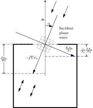
Figure 1: Resonant cavity with aperture. An external plane wave crosses the aperture and impinges on a corner reflector which sends back a reflected wave, providing a maximum of spatial phase variation in this direction. In contrast, the gradient of the phasor amplitude, which is another form of phase variation, has its maximum in the orthogonal direction.

For example, consider a plane wave impinging on the aperture of a cavity, as it is shown in Figure 1. The external plane wave crosses the aperture and impinges on a corner reflector which sends back a reflected wave, providing a maximum of $\psi_{s}$ variation in this direction. In contrast, the gradient of the phasor amplitude, which is another form of phase variation, has its maximum in the orthogonal direction. The gradients would follow straight lines in the space and differential squares would become aligned with the gradients. This conformal mapping has an associated Pólya complex potential (using $j$ instead of $i$ because we are on the $1j$ plane). In this case we have a uniform flow of phase and the complex potential is $f=2\pi(\bar{x}+j\bar{y})+\text{constant}$. Thus the velocity of the fluid $f^{\prime}$ is everywhere constant and equals $2\pi$ in terms of adimensional space coordinates. Using this terminology, stream lines appear when $\psi_{s}=0,\pm\kappa,\pm 2\kappa,\ldots$ while equipotencial lines appear when $\phi_{s}=0,\pm\kappa,\pm 2\kappa$ where $\kappa$ is a constant. The speed of the flow is represented by the crowding together of the streamlines. No fluid can cross them. While equipotential lines would represent a velocity potential.

The condition for the real part of $\nabla\cdot\nabla$ in (27) is also important:

$$\nabla^{2}U_{s}=\left(\frac{\nabla^{2}A_{s}}{A_{s}}-(\nabla\psi_{s})^{2}\right)U_{s}=-(2\pi)^{2}U_{s}$$ (31)

If we have a Pólya complex potential, then $A_{s}$ must also be harmonic, and therefore $\nabla^{2}A_{s}=0$. This restriction together with ($\ref{eq:nabla2comparison})$ implies that:

$$(\nabla\psi_{s})^{2}=(2\pi)^{2}$$ (32)

In our example, a monochromatic plane wave is assumed to impinge on the external surface of this aperture. In turn, the wave that crosses the aperture bounces in the inner corner reflector inside the cavity. As a consequence, there exists a strong reflection in the opposite direction so the gradient of spatial phase $\nabla\psi_{s}$ reaches its maximum which equals the wave number of the medium, satisfying (32) and therefore forcing $\nabla^{2}A_{s}=0$ which is consistent with a Pólya complex potential.

Figure 2: Images of subapertures seen from the aperture center. The aperture wall and the cavity roof are not depicted to show the sampling points. Almost zenithal view. There are three vertical layers with 72, $81\times 2$ and $81\times 2$ aperture images, 396 images in total and 1584 subapertures.

IV Verifiable consequences using divergence theorem

The Kirchhoff boundary conditions for the aperture have been found to yield remarkably accurate results and are widely used in practice in spite of their internal inconsistencies. So we consider unperturbed plane waves on the aperture surface. Additionally, the aperture provides an environment in which $\nabla A_{s}/A_{s}$ is expected to be non-zero due to the presence of evanescent modes. As stated in (30), $\nabla A_{s}$ and $\nabla\psi_{s}$ should be orthogonal when they are non-zero.

Applying the divergence theorem to (26):

$$\oiint_{S}U_{s}\left(\frac{\nabla A_{s}}{A_{s}}+j\nabla\psi_{s}\right)\cdot d\mathbf{s}=-(2\pi)^{2}\iiint_{V}U_{s}dv,$$ (33)

where $S$ is a closed surface with differential surface normal $d\mathbf{s}$, with modulus $ds$ and unit vector $\mathbf{n}$, bounding the volume $V$. (33) in terms of normal derivatives is therefore:

$$\oiint_{S}\!\!U_{s}\left(\frac{1}{A_{s}}\frac{\partial A_{s}}{\partial n}+j\frac{\partial\psi_{s}}{\partial n}\right)ds=-(2\pi)^{2}\iiint_{V}U_{s}dv,$$ (34)

According to the Helmholtz equivalency theorem[16], an aperture can be treated as a collection of secondary sources. In this context, the Kirchhoff boundary conditions have been found to yield remarkably accurate results and are widely used in practice in spite of their internal inconsistencies. The Kirchhoff solution is the arithmetic average of the two Rayleigh-Sommerfeld solutions which have consistent boundary conditions [17]. We consider plane waves on the aperture surface $S^{\prime}$, neglecting fringing effects, as first approximation. Under these conditions (34) can be reduced to:

$$\left(\frac{1}{A_{s}}\frac{\partial A_{s}}{\partial n}+j\frac{\partial\psi_{s}}{\partial n}\right)\!\!\iint_{S^{\prime}}U_{s}ds^{\prime}=-(2\pi)^{2}\!\iiint_{V}\!\!U_{s}dv,$$ (35)

where the first factor would be constant on the aperture surface $S^{\prime}$ due to the unperturbed plane wave approximation, therefore it can be expressed as follows:

$$\left(\frac{1}{A_{s}}\frac{\partial A_{s}}{\partial n}+j\frac{\partial\psi_{s}}{\partial n}\right)=\frac{-(2\pi)^{2}\iiint_{V}U_{s}dv}{\iint_{S^{\prime}}U_{s}ds^{\prime}}.$$ (36)

The argument of the right hand side of (36) can be simplified as follows:

$$\arg\left\{\frac{\iiint_{V}U_{s}dv}{\iint_{S^{\prime}}U_{s}ds^{\prime}}\right\} = \arg\left\{\iiint_{V}U_{s}dv\right\}$$ (37)

$$- \arg\left\{\iint_{S^{\prime}}U_{s}ds^{\prime}\right\},$$

where the limits of the last integral correspond to the aperture surface $S^{\prime}$. On this surface, the unperturbed plane wave approximation provides a linear phase distribution which is symmetric respect to the center of the aperture $(0,0,0)$ and therefore:

$$\arg\left\{\iint_{S^{\prime}}U_{s}ds^{\prime}\right\}=\arg\left\{U_{s}(0,0,0)\right\}=\psi_{s}(0,0,0).$$ (38)

The subtrahend of the right hand side of (37) takes out the influence of the actual value of $\psi_{s}(0,0,0)$. Therefore, without loss of generality, it will be considered hereafter that: $\psi_{s}(0,0,0)=0$ at the aperture center. The fact that $\psi_{s}(0,0,0)=0$ is of great importance because for each point within the cavity there exists only one phase $\psi_{s}(x,y,z)$ which is consistent with this phase at the aperture center. Moreover $\psi_{s}(x,y,z)$ can be calculated in advance using geometric information. In particular, after using $\psi_{s}(0,0,0)=0$ at the aperture center, the points inside the cavity have negative phase in order to represent an outgoing flow of standing waves, which is generated inside the cavity. Thus, with this new phase reference, (36) would be:

$$\left(\frac{1}{A_{s}}\frac{\partial A_{s}}{\partial n}-j\frac{\partial\psi_{s}}{\partial n}\right)=\frac{-(2\pi)^{2}\iiint_{V}A_{s}e^{-j\psi_{s}}dv}{\iint_{S^{\prime}}A_{s}e^{-j\psi_{s}}ds^{\prime}}.$$ (39)

The projection of $\frac{\nabla A_{s}}{A_{s}}-j\nabla\psi_{s}$ onto the unit normal $\mathbf{n}$ is shown in Figure 1 and is given by:

$$\frac{1}{A_{s}}\frac{\partial A_{s}}{\partial n}-j\frac{\partial\psi_{s}}{\partial n}=2\pi(-\sin\alpha-j\cos\alpha),$$ (40)

where the sense of $\nabla\psi_{s}$ is consistent with increasing phases in the sense of the outgoing flow and the sense of $\nabla{A_{s}}$ is due to an exponential decay of the amplitude in the outward direction. The real and the imaginary parts of this number represent the two legs of the same right triangle with hypotenuse $2\pi$, since we are assuming a uniform flow through the aperture. Therefore we obtain a verifiable consequence: this right triangle should determine the angle of incidence $\alpha$ of the original plane wave which comes from the external source:

$$\alpha=\frac{\pi}{2}-\arg\left\{\frac{\iiint_{V}A_{s}e^{-j\psi_{s}}dv}{\iint_{S^{\prime}}A_{s}e^{-j\psi_{s}}ds^{\prime}}\right\}.$$ (41)

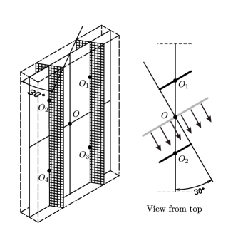
Figure 3: Contributions from an aperture can be divided into several subwindows.

As stated before, measurements inside the cavity must be performed in far field conditions. This requirement can be addressed treating the aperture as a collection of subapertures [18, 19]. For example, Figure 3 shows an aperture which has been divided in four subapertures. The zenithal view under far field approximation illustrates parallel propagation vectors from secondary sources radiating towards the target point. The superposition of the secondary sources at the subapertures is equivalent to the superposition of the secondary sources on the original aperture. In this example, the waves departing from secondary sources at subapertures $1$ and $3$ have longer path lengths than if they were to depart from the original aperture. However, in turn, subapertures $2$ and $4$ have a shorter pathlength. So the error of phase of each subaperture is compensated globally because under unperturbed plane wave approximation all the secondary sources have the same amplitude. As a conclusion, under far field conditions, the original aperture with null phase at its aperture center $O$ is equivalent to the four subapertures with null phase at their subaperture centers $O_{1}$, $O_{2}$, $O_{3}$ and $O_{4}$.

The presence of walls in the cavity has an important influence on the amplitude distribution inside the cavity. Walls behavior can be modeled by acoustic images of the real aperture that take into account reflections in the walls. In summary we substitute the effect of the walls by the effect of these equivalent apertures. Our aim is to find $\psi_{s}$ for each sampling point inside the cavity provided that $\psi_{s}=0$ at the aperture center. In order to find this phase, we need to identify which images must be taken into account. This approach simplifies the numerical solution because wall influence is treated using essentially the same tools that are needed to solve an isolated aperture.

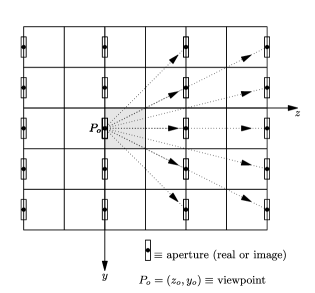
Figure 4: Only some acoustic images are source of waves that leave the cavity. Images with $z>0$ can send energy through the aperture because they are seen from the real aperture center $P_{o}$ looking inward.

However, not all the acoustic images of the real aperture in the six walls can be considered as sources of standing waves that impinge on the aperture surface in the outgoing direction. In the example shown in figure 4, only those images with $z>0$, or equivalently those apertures whose center is visible from the real aperture center viewpoint while looking inward should be taken into account. Those images with $z<0$ represent energy reflected in the aperture wall which does not leave the cavity and does not contribute to the outgoing flux of spatial waves. Only energy coming from the rest of the walls is eligible for modeling outgoing standing waves.

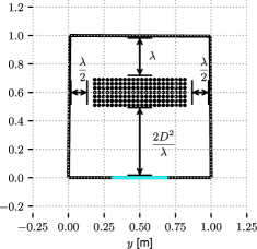
Figure 5: Sampling grid (height above the cavity ground of $0.545\text{\,}\mathrm{m}$).

V Experimental verification

The experimental verification of (23) and (41), which are backed up by the STIP, has been carried out by means of a resonant cavity with a squared aperture centered on the frontal wall of the cavity. A high-fidelity tweeter located outside the cavity radiated a pure tone with $\lambda=$0.3\text{\,}\mathrm{m}$$ through this aperture. The aperture was surrounded by an acoustic adsorbing material to prevent waves from entering the cavity other than through the aperture. The cavity was approximately a cube of edge $1\text{\,}\mathrm{m}$ although three of the four vertical faces were slightly rotated so that opposite faces were not parallel and consequently the interference pattern inside the cavity were more chaotic. A microphone (Earthworks M23) with a typical sensitivity of $34\text{\,}\mathrm{mV}\text{\,}{\mathrm{Pa}}^{-1}$ and uniform polar pattern was used. Its unique circuitry excludes the transconductance of the input FET from the overall gain structure. This means the sensitivity remains very stable when the microphone is subjected to variations in ambient temperature. The microphone was connected to a phantom power supply (Triton Audio True Phantom) with low noise components to achieve low distortion and improve the signal-to-noise ratio. The microphone signal was made available to a dynamic signal analyzer (HP 35670A) by means of an impedance transformer with $110\text{\,}\mathrm{\SIUnitSymbolOhm}$ input and $75\text{\,}\mathrm{\SIUnitSymbolOhm}$ output. For each sample, the analyzer averaged 5 time records using power averaging mode.

The microphone was carried on a rail guided vehicle to take spatial samples of acoustic intensity level inside the cavity. This vehicle was driven by three stepper motors, controlled by a laptop which dealt with the synchronization of measurements and displacements. The external acoustic source was also moved by means of another rail-guided vehicle. The source begins its motion in front of the center of the aperture, at a distance of $1.2\text{\,}\mathrm{m}$. Its trajectory was parallel to the aperture surface using discrete increments of $5\text{\,}\mathrm{cm}$. A servomotor was used to point the tweeter to the center of the aperture after each step automatically. Temperature and humidity conditions were also monitored in order to detect variations during the experiment. In addition a second microphone was placed outside the cavity at a fixed location to verify the absence of other external acoustic sources.

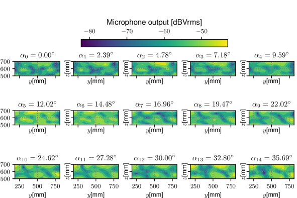
Figure 6: Measurements inside the cavity. Source location $y_{s}=0.5-0.05n\,\text{[m]},z_{s}=1.2\,\text{[m]}$ with $n=0,1,2,\ldots,14$. Angle of incidence $\alpha_{n}$.

Under ordinary conditions, there are temperature and humidity variations in the cavity over time that modify the wavelength of the acoustic field during the experiment. In order to avoid those wavelength variations, the temporal frequency $f$ of the wave generator was tuned for each sample in order to keep the wavelength $\lambda$ constant. This is possible using $f=v/\lambda$, where $f$ is the temporal frequency, $v$ is the speed of sound and $\lambda$ is a constant. In particular, we calculated the speed of sound in humid air as a function of the instantaneous temperature, relative humidity and pressure [20]. The saturation vapor pressure was taken from [21].

The sampling grid to measure sound intensity inside the cavity had 154 measurement points, as shown in Figure 5. We treat the aperture as a collection of 4 sub-apertures. Each sub-aperture is a square with side $19.5\text{\,}\mathrm{cm}$, each one satisfying the conventional far-field criteria. Therefore the distance from the sampling grid to the sub-apertures is:

$$\frac{2D^{2}}{\lambda}\approx$0.51\text{\,}\mathrm{m}$,$$ (42)

where the diagonal of each sub-aperture is $D\approx$0.276\text{\,}\mathrm{m}$$ and $\lambda=$0.3\text{\,}\mathrm{m}$$ is the wavelength.

The microphone and the rail-guided vehicle inside the cavity occupy some space, so there are points near the walls which are out of reach. Anyway, the measurements taken too close to the cavity walls are unreliable, as a result, some points must be left out of the sampling grid. The distance between samples is $0.1\lambda=$3\text{\,}\mathrm{cm}$$, which is the usual distance employed to retain enough information about the spatial distribution of the fields.

In general, in order to implement the divergence theorem, we would need a three-dimensional sampling volume inside the cavity instead of a two-dimensional sampling area. However, in our experimental setup, the direction of incidence was restricted to a horizontal plane, and under those conditions, the spatial distribution of the fields in a horizontal plane near the center of the cavity is assumed to contain enough information to estimate the angle of incidence. This assumption is based on our previous experiments [18, 19]. In those previous works we found that two-dimensional sampling areas in far field conditions provide an electric field envelope Cumulative Distribution Function (CDF) which identifies statistically the angle of incidence, independently of the precise location of each sample and regardless of not covering all the space near the cavity walls.

The lateral walls of the experimental cavity are not parallel as shown in Figure 5. Thus lateral images are seen from the real aperture center in contrast with the previous example in Figure 4. In turn, those lateral images have very close images due to the wall of the real aperture. But given that this second row of images are behind the real aperture, they are not seen directly from the real aperture. However, their reflections on the back wall, opposite to the aperture wall are necessary to represent certain geometrical conditions of the phase of the outgoing signal due to the lack of parallelism between walls. This is the reason why some images have a close duplicate in the layers of images which represent the back wall effect in Figure 2, which includes all the images taken into account. It is not necessary to include all the images which are seen from the real aperture. Although there is an infinite number of them, not all the images are equally important. For example those that are far away have a weaker influence and their geometrical description tends to be more prone to cumulative errors.

Our experimental approximation to (41) for the angle of incidence $\alpha$ is:

$$\alpha=\frac{\pi}{2}-\arg\left\{\sum_{n\mathop{=}1}^{N}|U_{s}(n)|\,e^{j\psi_{n}}\right\}$$ (43)

where $N=154$ is the total number of sampling points, $|U_{s}(n)|$ is the amplitude measured in the $n^{\rm{th}}$ sampling point and $\psi_{n}$ is the phase calculated assuming $\psi_{s}=0$ at the supaperture center and the same amplitude in every image. In particular, the expression for $\psi_{n}$ can be calculated in anticipation using only geometrical data and is calculated only once:

$$\psi_{n}=\arg\left\{\sum_{m\mathop{=}1}^{M}\frac{e^{-j\frac{2\pi}{\lambda}d_{nm}}}{d_{nm}}\right\},$$ (44)

where $\lambda=$0.3\text{\,}\mathrm{m}$$ is the wavelength, $d_{mn}$ is the distance between the $n^{\rm{th}}$ sampling point and the center of the $m^{\rm{th}}$ subaperture image. $M=1584$ is the total number of images which are taken into account (shown in Figure 2).

Ideal result	0.0	2.4	4.8	7.1	9.5	11.8	14.0	16.3	18.4	20.6	22.6	24.6	26.6	28.4	30.3
Regression 1	0.5	2.8	5.1	7.3	9.6	11.8	14.0	16.2	18.3	20.3	22.3	24.3	26.2	28.0	29.7
Regression 2	2.1	4.4	6.6	8.8	11.0	13.1	15.2	17.3	19.3	21.3	23.2	25.1	26.9	28.7	30.4
Raw result 1	4.0	7.7	7.5	6.3	2.0	2.0	6.5	15.3	25.5	29.0	26.9	23.7	23.5	27.5	29.0
Raw result 2	4.5	14.5	12.3	6.6	4.0	3.5	4.8	13.1	21.8	26.0	25.3	25.5	28.5	32.2	31.0

Table 2: Numerical comparison between the angles of incidence in degrees, the raw angles obtained from (43) and the estimated angles using a linear regression of the raw angles.

VI Results and conclusions

The experimental results are summarized in Figure 7. We provide a comparison between the real angles of incidence and those predicted by means of (43). Our sampling region does not cover all the space inside the cavity and there are several approximations, therefore it is not possible to obtain an accurate prediction for each isolated location of the external source. However, by using a linear regression we can compensate the errors.

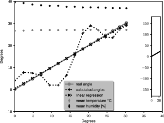
Figure 7: Comparison between the real angle of incidence and the calculated ones. The prediction is finally fitted using a linear regression. The inset shows a general view covering all the possible values.

The fitted prediction follows with accuracy the external source displacements of $\lambda/6$ using a $3.3\lambda\times 3.3\lambda$ cavity. All the calculated angles were the result of considering a fixed set of 243936 hypercomplex numbers that provide a description of the geometry of the cavity in terms of the location of the sampling points.

If (43) were not related to the angle of incidence we would expect a much more chaotic distribution of predictions. In fact, the argument of a random complex number could have any value in $[$$,$$)$. In contrast, instead of a chaotic distribution we obtain a set of points oscillating around a regression line which predicts fairly close the ideal dataset. Moreover, the same experiment was repeated, with different profiles of temperature and humidity. Due to the environmental variations, each realization of the same experiment provided a different prediction, however they were quite similar as can be seen in Table 2.

In conclusion, we have provided a mathematical formalism and a physical interpretation for solving the adimensional version of the wave equation in compliance with the Space-Time Interchangeability Principle, which in turn, is strongly backed by other well proven physical theories such as Relativity. This formalism has been validated by providing experimental data which confirm its predictions. The solution is based on quaternions and predicts additional forms of phase which are necessary to obtain a more complete description of the wave phenomena. Evanescent waves which are presently not fully understood play an important role in the experimental model. The concept of phase flow in terms of Pólya potential, helps to integrate the wave phenomena with other related physical phenomena, such as electrostatics and fluid motion. Although this work is limited to the wave equation, the background concept is the relationship between space and time and therefore could have far reaching consequences in other physical models.

References

- Altmann [1986] S. Altmann, Rotations, quaternions and double groups (Clarendon Press, 1986) pp. 9–28.
- Kravchenko [2003] V. V. Kravchenko, Applied Quaternionic Analysis (Heldermann, 2003).
- Penrose [2004] R. Penrose, The Road to Reality: A Complete Guide to the Laws of the Universe (Random House, 2004) pp. 201–203.
- Kantor and Solodovnikov [1989] I. L. Kantor and A. S. Solodovnikov, Hypercomplex numbers (Springer, 1989) pp. 41–51.
- Dixon [1994] G. Dixon, Division algebras: octonions, quaternions, complex numbers, and the algebraic design of physics (Springer, 1994) pp. 31–49.
- Ward [1997] J. Ward, Quaternions and Cayley Numbers (Springer, 1997) pp. 105–213.
- Moisil and Théodoresco [1931] G. Moisil and N. Théodoresco, Functions holomorphes dans l’espace, Mathematica Cluj 5, 142 (1931).
- Gürlebeck and Sprössig [1997] K. Gürlebeck and W. Sprössig, Quaternionic and Clifford Calculus for Physicists and Engineers (John Wiley & Sons, 1997) pp. 37–74.
- Kravchenko and Shapiro [1996] V. V. Kravchenko and M. Shapiro, Integral Representations for Spatial Models of Mathematical Physics (Longman, 1996) pp. 1–11.
- Langtangen and Pedersen [2016] H. P. P. Langtangen and G. K. Pedersen, Scaling of Differential Equations (Springer, 2016) p. 71.
- Tahir-Kheli [2018] R. Tahir-Kheli, Ordinary Differential Equations: Mathematical Tools for Physicists, 1st ed. (Springer, 2018).
- Needham [1998] T. Needham, Visual Complex Analysis (Clarendon Press, 1998).
- Arthur [2011] J. W. Arthur, Understanding Geometric Algebra for Electromagnetic Theory (John Wiley & Sons, 2011).
- Hestenes and Lasenby [2015] D. Hestenes and A. Lasenby, Space-Time Algebra (Birkhäuser, 2015) pp. 31–33.
- Polya and Latta [1974] G. Polya and G. Latta, Complex Variables (John Wiley & Sons, 1974).
- Baker and Copson [1939] B. B. Baker and E. T. Copson, The Mathematical Theory of Huygens’ Principle (Oxford, University Press, 1939) p. 23.
- Goodman [1968] J. Goodman, Introduction to Fourier Optics Goodman (McGraw-Hill, 1968) pp. 40–51.
- Blas et al. [2008] J. Blas, P. Fernández, R. M. Lorenzo, E. J. Abril, S. Mazuelas, A. Bahillo, and D. Bullido, Progress In Electromagnetics Research 85, 147 (2008).
- Blas et al. [2009] J. Blas, R. M. Lorenzo, P. Fernández, E. J. Abril, A. Bahillo, S. Mazuelas, and D. Bullido, Progress In Electromagnetics Research 91, 101 (2009).
- Cramer [1993] O. Cramer, The variation of the specific heat ratio and the speed of sound in air with temperature, pressure, humidity, and co2 concentration, The Journal of the Acoustical Society of America 93, 2510 (1993).
- Davis [1992] R. S. Davis, Equation for the determination of the density of moist air (1981/91), Metrologia 29, 67 (1992).