Quadratically enriched tropical intersections

Abstract

Using tropical geometry one can translate problems in enumerative geometry to combinatorial problems. Thus tropical geometry is a powerful tool in enumerative geometry over the complex and real numbers. Results from $\mathbb{A}^{1}$-homotopy theory allow to enrich classical enumerative geometry questions and get answers over an arbitrary field. In the resulting area, $\mathbb{A}^{1}$-enumerative geometry, the answer to these questions lives in the Grothendieck-Witt ring of the base field $k$. In this paper, we use tropical methods in this enriched set up by showing Bézout’s theorem and a generalization, namely the Bernstein-Kushnirenko theorem, for tropical hypersurfaces enriched in $\operatorname{GW}(k)$.

1 Introduction

Classically, Bézout’s theorem states that any $n$ hypersurfaces in $\mathbb{P}^{n}_{\mathbb{C}}$ of degrees $d_{1},\ldots,d_{n}$ that intersect transversally, intersect in $d_{1}\cdot\ldots\cdot d_{n}$ points. The count is invariant of the choice of hypersurfaces. This invariance breaks down if we replace the base field $\mathbb{C}$ by a non-algebraically closed field $k$. For example for $k=\mathbb{R}$ some of the intersections might only be defined over the complex numbers. Motivated by results from $\mathbb{A}^{1}$-homotopy theory there is a new way of counting geometric objects when the base field $k$ is not algebraically closed. The resulting count is valued in the Grothendieck-Witt ring $\operatorname{GW}(k)$ of $k$. This way of counting restores the invariance in the “relatively oriented” case.

Recall that the Grothendieck-Witt ring $\operatorname{GW}(k)$ is generated by $\left\langle a\right\rangle$ with $a\in k^{\times}/(k^{\times})^{2}$ and that $h\coloneqq\left\langle 1\right\rangle+\left\langle-1\right\rangle$ denotes the hyperbolic form. In [McK21] Stephen McKean proves Bézout’s theorem enriched in $\operatorname{GW}(k)$: Let $V_{1},\ldots,V_{n}$ be hypersurfaces in $\mathbb{P}^{n}_{k}$ defined by homogeneous polynomials $F_{1},\ldots,F_{n}$ of degrees $d_{1},\ldots,d_{n}$, respectively, such that $\sum_{i=1}^{n}d_{i}\equiv n+1\mod 2$. Assume that all the common zeros of $F_{1},\ldots,F_{n}$ lie in $U_{0}=\{x_{0}\neq 0\}\subset\mathbb{P}^{n}_{k}$ and set polynomials on the affine chart $f_{i}(x_{1},\ldots,x_{n})\coloneqq F_{i}(1,x_{1},\ldots,x_{n})$. Furthermore, assume that the hypersurfaces intersect transversally at every intersection point, then

$$\sum_{p\in V_{1}\cap\ldots\cap V_{n}}\operatorname{Tr}_{k(p)/k}\left\langle\det\operatorname{Jac}(f_{1},\ldots,f_{n})(p)\right\rangle=\frac{d_{1}\cdot d_{2}\cdots d_{n}}{2}\cdot h\in\operatorname{GW}(k).$$ (1)

In this paper we reprove (1) and generalize the result using tropical geometry. To do this, we define enriched tropical hypersurfaces. The definition is motivated by Viro’s patchworking.

Definition 1.1.

An enriched tropical hypersurface $\widetilde{V}=(V,(\alpha_{I}))$ in $\mathbb{R}^{n}$ is a tropical hypersurface $V$ in $\mathbb{R}^{n}$ together with an element $\alpha_{I}\in k^{\times}/(k^{\times})^{2}$ assigned to each connected component of $\mathbb{R}^{n}\setminus V$.

Recall that connected components of $\mathbb{R}^{n}\setminus V$ correspond to vertices in the dual subdivision of $V$. So we can alternatively assign coefficients $\alpha_{v}$ to each vertex $v$ in the dual subdivision of $V$. An enriched tropical hypersurface can be seen as a homotopy equivalence class of Viro polynomials associated to the dual subdivision of an embedded tropical hypersurface in $\mathbb{R}^{n}$ and a choice of coefficients in $k^{\times}$ for each vertex in the dual subdivision. These Viro polynomials are of the form

$$\sum_{I\in A}\alpha_{I}x^{I}t^{\varphi(I)}$$

where $A$ is a finite subset of $\mathbb{Z}^{n}$, $\alpha_{I}\in k^{\times}$ for any $I\in A$, $x=(x_{1},\ldots,x_{n})$ and $\varphi:A\rightarrow\mathbb{Q}$ is a convex function that assigns a rational number to each exponent $I\in A$. These Viro polynomials can be viewed as polynomials over the field of Puiseux series

$$k\{\{t\}\}=\left\{\sum_{i=i_{0}}^{\infty}c_{i}t^{\frac{i}{n}}\mid c_{i}\in k,i_{0}\in\mathbb{Z},n\in\mathbb{N}\right\}$$

over (the base field) $k$.

Let $\widetilde{V}_{1},\ldots,\widetilde{V}_{n}$ be $n$ enriched tropical hypersurfaces in $\mathbb{R}^{n}$ with Viro polynomials $f_{1},\ldots,f_{n}$ in $k\{\{t\}\}[x_{1},\ldots,x_{n}]$. Inspired by (1) we define the enriched intersection multiplicity of $\widetilde{V}_{1},\ldots,\widetilde{V}_{n}$ at an intersection point $p$ to be

$$\widetilde{\operatorname{mult}}_{p}(\widetilde{V}_{1},\ldots,\widetilde{V}_{n})\coloneqq\operatorname{Tr}_{E_{t}/k\{\{t\}\}}\left\langle\det\operatorname{Jac}(f_{1},\ldots,f_{n})(p)\right\rangle\in\operatorname{GW}(k\{\{t\}\})\cong\operatorname{GW}(k)$$ (2)

where $E_{t}$ is the coordinate ring of the closed subscheme of the points that tropicalize to $p$. Note that taking the rank of (2) recovers the classical (tropical) intersection multiplicity.

It is rather tedious to compute this enriched intersection multiplicity. The main theorem of this paper finds a purely combinatorial rule to determine it.

Definition 1.2.

Let $\Lambda^{\text{odd}}$ be the subset of $\mathbb{Z}^{n}$ consisting of tuples $(a_{1},\ldots,a_{n})$ with $a_{i}\equiv 1\mod 2$ for $i=1,\ldots n$. We call the elements of $\Lambda^{\mathrm{odd}}$ odd lattice points.

Our Main Theorem states that the enriched intersection multiplicity is determined by the coefficients of the odd vertices of the dual subdivision. To avoid confusion, we say that the vertices of a polytope that belong to a minimal generating set with respect to the convex hull are its corner vertices.

Theorem 1.3 (Main Theorem).

Let $P$ be the parallelepiped in the dual subdivision of the union $\widetilde{V}_{1}\cup\widetilde{V}_{2}\cup\ldots\cup\widetilde{V}_{n}$ corresponding to the intersection point $p$. Assume that the volume of $P$ equals $m$. Let $r$ be the number of corners of $P$ that are elements of $\Lambda^{\text{odd}}$. Then

$$\widetilde{\operatorname{mult}}_{p}(V_{1},\ldots,V_{n})=\sum_{v\text{ an odd corner of }P}\left\langle\epsilon(v)\alpha_{v}\right\rangle+\frac{m-r}{2}\cdot h\in\operatorname{GW}(k).$$

Here, $\alpha_{v}$ denotes the coefficient of the vertex $v$ and $\epsilon(v)$ is a sign determined by the intersection.

There is an easy proof for Bézout’s theorem for tropical curve (not enriched in $\operatorname{GW}(k)$) by Bernd Sturmfels: The intersection points of two tropical curves $C_{1}$ and $C_{2}$ with Newton polygons $\Delta_{d_{1}}$ and $\Delta_{d_{2}}$, respectively, correspond to parallelograms in the dual subdivision of $C_{1}\cup C_{2}$. The area of such a parallelogram is equal to the intersection multiplicity at the corresponding intersection point and the rest of the dual subdivision of $C_{1}\cup C_{2}$ consists of the dual subdivisions of $C_{1}$ and $C_{2}$. Thus the number of intersections counted with multiplicities is

$$\operatorname{Area}(\Delta_{d_{1}+d_{2}})-\operatorname{Area}(\Delta_{d_{1}})-\operatorname{Area}(\Delta_{d_{2}})=\frac{(d_{1}+d_{2})^{2}}{2}-\frac{d_{1}^{2}}{2}-\frac{d_{2}^{2}}{2}=d_{1}\cdot d_{2}.$$

This is a particular instance of a more general statement. Two tropical curves $C_{1}$ and $C_{2}$ in $\mathbb{R}^{2}$ of with Newton polygons $\Delta_{1}$ and $\Delta_{2}$, respectively, intersect in a number of points counted with multiplicities equal to the mixed volume

$$\operatorname{MVol}(\Delta_{1},\Delta_{2})=\operatorname{Area}(\Delta_{1}+\Delta_{2})-\operatorname{Area}(\Delta_{1})-\operatorname{Area}(\Delta_{2}),$$ (3)

where $\Delta_{1}+\Delta_{2}$ is the Minkowski sum of the polygons $\Delta_{1}$ and $\Delta_{2}$.

Two tropical curves embedded in $\mathbb{R}^{2}$ intersect tropically transversely if they intersect in a finite number of points and every point of the intersection belongs to an edge in each of the curves. A direct consequence of our Main Theorem 1.3 is that we can quadratically enrich Sturmfels’ proof for enriched tropical curves that intersect tropically transversally at every intersection point. Theorem 1.3 implies that the only non-hyperbolic contribution to (1) comes from odd points on the boundary of $\Delta_{1}+\Delta_{2}$ (see Proposition 6.1 and Corollary 6.5). Hence, we get the following.

Theorem 1.4.

Let $\widetilde{C}_{1}$ and $\widetilde{C}_{2}$ be two enriched tropical curves with Newton polygons $\Delta_{1}$ and $\Delta_{2}$, respectively. Assume that they intersect tropically transversally at every intersection point and that $\partial(\Delta_{1}+\Delta_{2})\cap\Lambda^{\mathrm{odd}}=\emptyset$. Then

$$\sum_{p\in\widetilde{C}_{1}\cap\widetilde{C}_{2}}\widetilde{\operatorname{mult}}_{p}(\widetilde{C}_{1},\widetilde{C}_{2})=\frac{\operatorname{MVol}(\Delta_{1},\Delta_{2})}{2}\cdot h\in\operatorname{GW}(k).$$

In particular, we recover (1) for curves, since the condition $d_{1}+d_{2}$ being odd implies that $\partial(\Delta_{d_{1}}+\Delta_{d_{2}})\cap\Lambda^{\mathrm{odd}}=\partial(\Delta_{d_{1}+d_{2}})\cap\Lambda^{\mathrm{odd}}=\emptyset$.

Corollary 1.5.

Let $\widetilde{C}_{1}$ and $\widetilde{C}_{2}$ be enriched tropical curves over $k$ of with Newton polygons $\Delta_{d_{1}}$ and $\Delta_{d_{2}}$, respectively. If $d_{1}+d_{2}\equiv 1\mod 2$, then

$$\sum_{p\in C_{1}\cap C_{2}}\widetilde{\operatorname{mult}}_{p}(\widetilde{C}_{1},\widetilde{C}_{2})=\frac{d_{1}\cdot d_{2}}{2}h\in\operatorname{GW}(k).$$

When $d_{1}+d_{2}\equiv 0\mod 2$, we are dealing with the non-relatively orientable case, in which the left hand side in (1) depends on choice of coefficients. However, the left hand side of (1) can not equal any element of $\operatorname{GW}(k)$. More precisely, we have the following possibilities for the intersection of two enriched tropical curves.

Corollary 1.6.

Let $\widetilde{C}_{1}$ and $\widetilde{C}_{2}$ be enriched tropical curves over $k$ with Newton polygons $\Delta_{d_{1}}$ and $\Delta_{d_{2}}$, respectively. If $\widetilde{C}_{1}$ and $\widetilde{C}_{2}$ intersect tropically transversally and $d_{1}+d_{2}\equiv 0\mod 2$, then

$$\sum_{p\in C_{1}\cap C_{2}}\widetilde{\operatorname{mult}}_{p}(\widetilde{C}_{1},\widetilde{C}_{2})=\frac{d_{1}\cdot d_{2}-\min(d_{1},d_{2})}{2}h+\left\langle a_{1},\dots,a_{\min(d_{1},d_{2})}\right\rangle\in\operatorname{GW}(k),$$

where $a_{1},\ldots,a_{\min(d_{1},d_{2})}$ can be any element in $k^{\times}/(k^{\times})^{2}$.

Sturmfels’ argument also works in higher dimensions (see [HS95]): Let $V_{1},\ldots,V_{n}$ be tropical hypersurfaces in $\mathbb{R}^{n}$ with Newton polytopes $\Delta_{1},\ldots,\Delta_{n}$. Then the number of intersection points counted with multiplicities equals the mixed volume

$$\operatorname{MVol}(\Delta_{1},\ldots,\Delta_{n})\coloneqq\text{coefficient of $\lambda_{1}\cdots\lambda_{n}$ in $R(\lambda_{1},\ldots,\lambda_{n})\coloneqq\operatorname{vol}(\lambda_{1}\Delta_{1}+\ldots+\lambda_{n}\Delta_{n})$.}$$ (4)

This agrees with (3) in dimension $2$.

We replace the relative orientation condition by a purely combinatorial condition, namely we assume that

$$\partial(\Delta_{1}+\ldots+\Delta_{n})\cap\Lambda^{\mathrm{odd}}=\emptyset.$$

In this case our Main Theorem 1.3 implies.

Corollary 1.7.

Let $\widetilde{V}_{1},\ldots,\widetilde{V}_{n}$ be $n$ tropical hypersurfaces with Newton polytopes $\Delta_{1},\ldots,\Delta_{n}$, respectively, such that $\partial(\Delta_{1}+\ldots+\Delta_{n})\cap\Lambda^{\mathrm{odd}}=\emptyset$. Assume that $\widetilde{V}_{1},\ldots,\widetilde{V}_{n}$ intersect tropically transversally at every point. Then

$$\sum_{p\in\widetilde{V}_{1}\cap\ldots\cap\widetilde{V}_{n}}\widetilde{\operatorname{mult}}_{p}(\widetilde{V}_{1},\ldots,\widetilde{V}_{n})=\frac{\operatorname{MVol}(\Delta_{1},\ldots,\Delta_{n})}{2}h\in\operatorname{GW}(k).$$

From this we can derive a quadratic enrichment of a Theorem of Bernstein and Kushnirenko.

Corollary 1.8 (Enriched Bernstein-Kushnirenko Theorem).

Let $f_{1},\ldots,f_{n}$ be Laurent polynomials in $n$ variables with Newton polytopes $\Delta_{1},\ldots,\Delta_{n}$, respectively. If ${\partial(\Delta_{1}+\ldots+\Delta_{n})\cap\Lambda^{\mathrm{odd}}=\emptyset}$, then

$$\sum_{z}\operatorname{Tr}_{k(z)/k}\left\langle\det\operatorname{Jac}(f_{1},\ldots,f_{n})(z)\right\rangle=\frac{\operatorname{MVol}(\Delta_{1},\ldots,\Delta_{n})}{2}h\in\operatorname{GW}(k).$$

Here, the sum runs over all solutions $z$ to $f_{1}=\ldots=f_{n}=0$ in $\operatorname{Spec}k[x_{1}^{\pm 1},\ldots,x_{n}^{\pm 1}]$.

1.1 Related work and the a general strategy for quadratically enriched tropical counts

In [MPS22] Markwig, Payne and Shaw use tropical methods to redo the quadratically enriched count of bitangents to a quartic curve by Larson-Vogt [LV19]. Their strategy is similar to ours, they also use enriched tropical curves: In many cases, questions in enumerative geometry can be solved by counting zeros of a general section of some vector bundle. This is the case for Bézout’s theorem and the count of bitangents to a quartic curve. Hence, these counts equal the degree of the Euler class of the respective vector bundles and their quadratic enrichments are the degree of the “$\mathbb{A}^{1}$-Euler class” of the respective vector bundles. There is a “Poincaré-Hopf Theorem” (see Theorem 2.15 for the classical Poincaré-Hopf Theorem) for the degree of the $\mathbb{A}^{1}$-Euler class of a vector bundle, that is, the degree of the $\mathbb{A}^{1}$-Euler class equals the sum of “local indices” at the zeros of a chosen section. One can write down explicit polynomials to compute these local indices and then interpret them tropically. In our case, the local index is what we call the enriched tropical multiplicity defined in (2) and its tropical interpretation is our Main Theorem 1.3.

1.2 Outline

We start by recalling the prerequisites from $\mathbb{A}^{1}$-enumerative geometry in section 2 and tropical geometry in section 3. In section 4 we prove our Main Theorem for tropical curves and generalize is to any dimension in section 5. In section 6 we use our Main theorem to prove the enriched tropical Bézout theorem and the enriched Bernstein-Kushnirenko theorem.

1.3 Acknowledgements

Both authors have been supported by the ERC programme QUADAG. This paper is part of a project that has received funding from the European Research Council (ERC) under the European Union’s Horizon 2020 research and innovation programme (grant agreement No. 832833).

The second author acknowledges the support of the Centre for Advanced Study at the Norwegian Academy of Science and Letters in Oslo, Norway, which funded and hosted the research project “Motivic Geometry” during the 2020/21 academic year.

The second author would like to thank the Isaac Newton Institute for Mathematical Sciences, Cambridge, for support and hospitality during the programme “K-theory, algebraic cycles and motivic homotopy theory” where work on this paper was undertaken. This work was supported by EPSRC grant no EP/R014604/1.&#34.

We would like to thank Marc Levine, Stephen McKean and Kris Shaw for fruitful discussions.

2 Introduction to $\mathbb{A}^{1}$-enumerative geometry

In $\mathbb{A}^{1}$-enumerative geometry one uses machinery from $\mathbb{A}^{1}$-homotopy theory to enrich classical results from enumerative geometry yielding results over an arbitrary field $k$. In this section, we introduce one way of doing this following the work of Jesse Kass and Kirsten Wickelgren in [KW21, KW19].

2.1 The Grothendieck-Witt ring

The enriched enumerative results will be valued in the Grothendieck-Witt ring. We recall the definition of $\operatorname{GW}(R)$ where $R$ is a commutative ring with $1$.

Definition 2.1.

The Grothendieck-Witt ring $\operatorname{GW}(R)$ of a ring $R$ is the group completion of the semi-ring of isometry classes of non-degenerate symmetric bilinear forms over $R$ under the direct sum $\oplus$ and tensor product $\otimes$.

We are mainly interested in the case when $R$ is a field $k$ of characteristic not equal to $2$ in which case we have a nice presentation of $\operatorname{GW}(k)$: Let $k^{\times}=k\setminus\{0\}$ be the set of units in $k$. If $\operatorname{char}k\neq 2$, any form can be diagonalized, i.e., for any symmetric bilinear form $\beta:V\times V\rightarrow k$. Hence, we can find a basis for the $k$-vector space $V$, such that

$$\beta((x_{1},\ldots,x_{n}),(y_{1},\ldots,y_{n}))=a_{1}x_{1}y_{1}+\ldots+a_{n}x_{n}y_{n}$$ (5)

for some $a_{1},\ldots,a_{n}\in k^{\times}$ in this basis. Also note that if we replace one of the $a_{i}$ by $a_{i}b^{2}$ for some $b\in k^{\times}$, the resulting form is in the same isometry class as $\beta$. Thus the form $\beta$ above (5) can be expressed as the direct sum of $n$ symmetric bilinear form on a one-dimensional $k$-vector space. Indeed $\operatorname{GW}(k)$ is generated by the classes of bilinear forms

$$\left\langle a\right\rangle\colon k\times k\rightarrow k\text{, }(x,y)\mapsto axy$$

for $a\in k^{\times}/(k^{\times})^{2}$ (since classes in $\operatorname{GW}(k)$ are non-degenerate, we need $a\neq 0$) subject to the following two relations

1. $\left\langle a\right\rangle\left\langle b\right\rangle=\left\langle ab\right\rangle$ for $a,b\in k^{\times}$

2. $\left\langle a\right\rangle+\left\langle b\right\rangle=\left\langle a+b\right\rangle+\left\langle ab(a+b)\right\rangle$ for $a,b,a+b\in k^{\times}$.

We use the notation $\left\langle a_{1},\ldots,a_{s}\right\rangle\coloneqq\left\langle a_{1}\right\rangle+\ldots+\left\langle a_{s}\right\rangle\in\operatorname{GW}(k)$.

Definition 2.2.

We write $h$ for the hyperbolic form, that is the form on a $2$-dimensional $k$-vector space (or free rank $2$ R-module over $R$ when $R$ is not a field), with Gram matrix $\begin{pmatrix}0&1\\ 1&0\end{pmatrix}$.

Remark 2.3.

1. Assume $a$ is a unit in $R$, then the class of the symmetric bilinear form on a rank $2$ $R$-module defined by $\begin{pmatrix}0&a\\ a&0\end{pmatrix}$ equals $h$.

2. If $k$ is a field of characteristic not equal to $2$, then after diagonalizing, we get that the hyperbolic form equals

   $$h=\left\langle 1\right\rangle+\left\langle-1\right\rangle.$$

   Furthermore, one can deduce from relation $2$ above that for $a\in k^{\times}$ the equality

   $$\left\langle a\right\rangle+\left\langle-a\right\rangle=\left\langle 1\right\rangle+\left\langle-1\right\rangle=h$$

   holds in $\operatorname{GW}(k)$.

Definition 2.4.

We say that the rank of a symmetric bilinear form

$$\beta:V\times V\rightarrow R$$

is the rank of the $R$-module $V$.

Taking the rank extends to a homomorphism

$$\operatorname{rank}:\operatorname{GW}(R)\rightarrow\mathbb{Z}.$$

Example 2.5.

Let $k=\mathbb{C}$. Since $\mathbb{C}$ is algebraically closed, there is only one generator $\left\langle 1\right\rangle\in\operatorname{GW}(k)$ and thus $\operatorname{GW}(k)\cong\mathbb{Z}$ where the isomorphism is the rank homomorphism. In particular, results in classical enumerative geometry coincide with the counts enriched in $\operatorname{GW}(k)$ for an algebraically closed field $k$ by taking the rank.

Example 2.6.

For $k=\mathbb{R}$, $\operatorname{GW}(k)$ has two generators, namely $\left\langle 1\right\rangle$ and $\left\langle-1\right\rangle$. In fact, an element in $\operatorname{GW}(\mathbb{R})$ is completely determined by its rank and its signature.

Example 2.7.

The Grothendieck-Witt ring of the field $k\{\{t\}\}$ of Puiseux series over $k$ is isomorphic to $\operatorname{GW}(k)$. This is because $k\{\{t\}\}^{\times}/(k\{\{t\}\}^{\times})^{2}=k^{\times}/(k^{\times})^{2}$. More precisely when $a_{m}\in k^{\times}$,

$$\sum_{i=m}^{\infty}a_{i}t^{\frac{i}{n}}=a_{m}\cdot\left(t^{\frac{m}{n}}+\sum_{i=m+1}^{\infty}\frac{a_{i}}{a_{m}}t^{\frac{i}{n}}\right)$$

and $\left(t^{\frac{m}{n}}+\sum_{i=m+1}^{\infty}\frac{a_{i}}{a_{m}}t^{\frac{i}{n}}\right)$ is a square in $k\{\{t\}\}$. So $\sum_{i=m}^{\infty}a_{i}t^{\frac{i}{n}}$ equals $a_{m}$ in $k\{\{t\}\}^{\times}/(k\{\{t\}\}^{\times})^{2}$. This yields the following isomorphism

$$\operatorname{In}\colon\begin{array}[]{ccc}\operatorname{GW}\left(k\{\{t\}\}\right)&\longrightarrow&\operatorname{GW}\left(k\right)\\ \left\langle\sum_{i=m}^{\infty}a_{i}t^{\frac{1}{n}}\right\rangle&\longmapsto&\left\langle a_{m}\right\rangle\end{array}$$

sending a generator to its initial.

2.1.1 The Witt ring

A non-degenerate symmetric bilinear form $\beta:V\times V\rightarrow R$ over a ring $R$ is split if there exists a submodule $N\subset V$ such that $N$ is a direct summand of $V$ and $N$ is equal to its orthogonal complement $N^{\bot}$. We say that two non-degenerate symmetric bilinear forms $\beta\colon V\times V\rightarrow R$ and ${\beta^{\prime}\colon V^{\prime}\times V^{\prime}\rightarrow R}$ are stably equivalent if there exist split symmetric bilinear forms $s$ and $s^{\prime}$ such $\beta\oplus s\cong\beta^{\prime}\oplus s^{\prime}$.

Definition 2.8.

The Witt ring of $R$ is the set of classes of stably equivalent non-degenerate symmetric bilinear forms with addition the direct sum $\oplus$ and multiplcation the tensor product $\otimes$.

Remark 2.9.

If $R$ is a field of characteristic not equal to $2$, then the split non-degenerate symmetric bilinear forms are exactly the multiples of the hyperbolic form $h$. Recall that in this case we have that $\langle a\rangle+\langle-a\rangle=h$ for any unit $a$ and hence

$$\operatorname{W}(k)\coloneqq\frac{\operatorname{GW}(k)}{\mathbb{Z}\cdot h}.$$

More generally, if $R$ is local and $2$ is invertible then an element of $\operatorname{GW}(R)$ is completely determined by its rank and element of $\operatorname{W}(R)$.

Example 2.10.

The Witt ring of $\mathbb{C}$ is isomorphic to $\mathbb{Z}/2\mathbb{Z}$.

2.1.2 Trace

Assume that $R$ is a commutative ring. We are particularly interested in the case that $R$ is a finite étale $k$-algebra. For a finite projective $R$-algebra $L$ one can define the trace $\operatorname{Tr}_{L/R}:L\rightarrow R$ that sends $b\in L$ to the trace of the multiplication map $m_{b}(x)=b\cdot x$. If $L$ is étale over $R$ this induces the trace map $\operatorname{Tr}_{L/R}\colon\operatorname{GW}(L)\rightarrow\operatorname{GW}(R)$ which sends the class of a bilinear form $\beta\colon V\times V\rightarrow L$ over $L$ to the form

$$V\times V\xrightarrow{\beta}L\xrightarrow{\operatorname{Tr}_{L/R}}R$$

over $R$.

We will compute several trace forms in our main result. So we already collect some facts and computations about the trace form here. Let $E$ be a finite étale $R$-algebra. Then

1. If $R=k$ is a field, then $E=L_{1}\times\ldots\times L_{s}$ for some finite separable field extensions $L_{1},\ldots,L_{s}$ of $k$ and the trace map $\operatorname{Tr}_{E/k}:E\rightarrow k$ equal to the sum of field traces $\operatorname{Tr}_{E/k}=\sum_{i=1}^{s}\operatorname{Tr}_{L_{i}/k}$.

2. $\operatorname{Tr}_{E/R}$ is $R$-linear.

3. Let $F$ be a finite étale $E$-algebra. Then

   $$\operatorname{Tr}_{F/R}=\operatorname{Tr}_{E/R}\circ\operatorname{Tr}_{F/E}.$$

From now on let $k$ be a field.

Lemma 2.11.

Let $L$ be a finite étale $k$-algebra. Let $E=\frac{L[x]}{(x^{m}-D)}$m for some $D\in L$, and assume that $E$ is étale over $L$. Then $\operatorname{Tr}_{E/L}(1)=m$ and $\operatorname{Tr}_{E/L}(x^{s})=0$ for $s\in\{1,\ldots,m-1\}$.

Proof.

We have the following $L$-basis for $E$: $1,x,x^{2},\ldots,x^{m-1}$. Recall that $\operatorname{Tr}_{E/L}(a)$ for $a\in E$ is the trace of the $L$-linear map $m_{a}:E\rightarrow E$ defined by $m_{a}(y)=a\cdot y$. So we are looking for the matrix of $m_{a}$ with respect to the basis $1,x,\ldots,x^{m-1}$.

1. If $a=1$, then this matrix is the identity matrix and its trace equals the $L$-dimension of $E$, namely $m$.

2. If $a=x^{s}$ for some $s\in\{1,\ldots,m-1\}$, then every entry of the diagonal of this matrix equals $0$.

∎

Since the trace $\operatorname{Tr}_{E/L}$ is $L$-linear, Lemma 2.11 tells us what $\operatorname{Tr}_{E/L}(a)$ is for any element $a\in E$ in case $E=\frac{L[x]}{(x^{m}-D)}$.

Lemma 2.12.

Let $E$ be a finite étale $R$-algebra of rank $m$. Then $\operatorname{Tr}_{E/R}(h)=m\cdot h$.

Proof.

This follows directly from the fact that the hyperbolic form $h$ is split. ∎

Proposition 2.13.

Let $L$ be a finite étale $k$-algebra and let $E=\frac{L[x]}{(x^{m}-D)}$, for some $D\in L$. Further, assume that $\operatorname{char}k$ does not divide $m$. Then for $a\in L$ we get

1. $\operatorname{Tr}_{E/L}(\left\langle m\cdot a\right\rangle)=\begin{cases}\left\langle a\right\rangle+\frac{m-1}{2}h&m\text{ odd}\\ \left\langle a\right\rangle+\left\langle a\cdot D\right\rangle+\frac{m-2}{2}h&m\text{ even.}\end{cases}$

2. $\operatorname{Tr}_{E/L}(\left\langle m\cdot a\cdot x\right\rangle)=\begin{cases}\left\langle a\cdot D\right\rangle+\frac{m-1}{2}h&m\text{ odd}\\ \frac{m}{2}h&m\text{ even.}\end{cases}$

Proof.

We have the following $L$-basis for $E$: $1,x,\ldots,x^{m-1}$. Let $M=(M_{ij})$ be the Gram matrix of $\operatorname{Tr}_{E/L}(\left\langle m\cdot a\right\rangle)$. Then the $(i,j)$th entry $M_{ij}$ of $M$ equals $\operatorname{Tr}_{E/L}(m\cdot a\cdot b_{i}\cdot b_{j})=\operatorname{Tr}_{E/L}(m\cdot a\cdot x^{i-1}\cdot x^{j-1})$, where $b_{i}=x^{i-1}$ is the $i$th basis element of the chosen $L$-basis of $L$. In particalur, we have

$$M_{ij}=\begin{cases}m^{2}\cdot a&\text{if }i=j=1\\ m^{2}\cdot a\cdot D&\text{if }i+j=m+1\\ 0&\text{otherwise}\end{cases}$$

by Lemma 2.11 and thus the Gram matrix of $\operatorname{Tr}_{E/L}(\left\langle m\cdot a\right\rangle)$ looks like

$$M=\begin{pmatrix}m^{2}\cdot a&0&\ldots&\ldots&\ldots&0\\ 0&\ldots&\ldots&\ldots&0&m^{2}\cdot a\cdot D\\ \ldots&\ldots&\ldots&\ldots&m^{2}\cdot a\cdot D&0\\ \ldots&\ldots&\ldots&\iddots&\ldots&\ldots\\ \ldots&0&m^{2}\cdot a\cdot D&\ldots&\ldots&\ldots\\ 0&m^{2}\cdot a\cdot D&0&\ldots&\ldots&0\end{pmatrix}.$$

By Remark 2.3 this is equivalent in $\operatorname{GW}(L)$ to $\left\langle a\right\rangle+\frac{m-1}{2}h$ if $m$ is odd, or to $\left\langle a\right\rangle+\left\langle a\cdot D\right\rangle+\frac{m-2}{2}h$ if $m$ is even. Now let $M$ be the Gram matrix of $\operatorname{Tr}_{E/L}(\left\langle m\cdot a\cdot x\right\rangle)$. Then the $(i,j)$-th entry equals

$$M_{ij}=\begin{cases}m^{2}\cdot a\cdot D&\text{if }i+j=n\\ 0&\text{otherwise.}\end{cases}$$

by Lemma 2.11 and we get that

$$M=\begin{pmatrix}0&0&\ldots&\ldots&\ldots&m^{2}\cdot a\cdot D\\ 0&\ldots&\ldots&\ldots&m^{2}\cdot a\cdot D&0\\ \ldots&\ldots&\ldots&m^{2}\cdot a\cdot D&0&0\\ \ldots&\ldots&\ldots&\ldots&\ldots&\ldots\\ 0&m^{2}\cdot a\cdot D&0&\ldots&\ldots&\ldots\\ m^{2}\cdot a\cdot D&0&\ldots&\ldots&\ldots&0\end{pmatrix}$$

which is the Gram matrix of a quadratic form with class in $\operatorname{GW}(L)$ equal to $\left\langle a\cdot D\right\rangle+\frac{m-1}{2}h$ if $m$ is odd, or to $\frac{m}{2}h$ if $m$ is even, by Remark 2.3. ∎

2.2 The $\mathbb{A}^{1}$-degree

$\mathbb{A}^{1}$-homotopy theory is a new branch of mathematics in which one aims to apply techniques from homotopy theory to the category of smooth algebraic varieties over a field $k$. Most constructions from classical homotopy theory work in this set up. In particular, we have an analog of the Brouwer degree. Recall (for example from [Hat02]) that the Brouwer degree from classical topology is an isomorphism from the homotopy classes of the endomorphisms of the $n$-sphere to the integers

$$\deg:[S^{n},S^{n}]\overset{\cong}{\rightarrow}\mathbb{Z}$$

for $n\geq 1$. Morel defines the $\mathbb{A}^{1}$-analog in [Mor12]. His $\mathbb{A}^{1}$-degree assigns an element of $\operatorname{GW}(k)$ to an $\mathbb{A}^{1}$-homotopy class of an endomorphism of the motivic sphere $\mathbb{P}^{n}_{k}/\mathbb{P}^{n-1}_{k}$

$$\deg^{\mathbb{A}^{1}}:[\mathbb{P}^{n}_{k}/\mathbb{P}^{n-1}_{k},\mathbb{P}^{n}_{k}/\mathbb{P}^{n-1}_{k}]_{\mathbb{A}^{1}}\rightarrow\operatorname{GW}(k).$$

Just like for the classical Brouwer degree, the $\mathbb{A}^{1}$-degree splits up as a sum of local $\mathbb{A}^{1}$-degrees. We refer to [KW19] for the definition of the local $\mathbb{A}^{1}$-degree and merely recall some of their formulas to compute the local $\mathbb{A}^{1}$-degree $\deg_{x}f$ of a map $f:\mathbb{A}^{n}_{k}\rightarrow\mathbb{A}^{n}_{k}$ at an isolated zero $x$.

2.2.1 Formulas for the local $\mathbb{A}^{1}$-degree

Assume $f:\mathbb{A}^{n}_{k}\rightarrow\mathbb{A}^{n}_{k}$ has an isolated $k$-rational zero $x$. Furthermore, assume that the determinant of the Jacobian $\operatorname{Jac}(f)$ of $f$ at $x$ does not vanish. In this case the local $\mathbb{A}^{1}$-degree at $x$ equals

$$\deg^{\mathbb{A}^{1}}_{x}f=\left\langle\det\operatorname{Jac}f(x)\right\rangle\in\operatorname{GW}(k).$$ (6)

Example 2.14.

Let $f:\mathbb{A}^{1}_{k}\rightarrow\mathbb{A}^{1}_{k}$ be defined by $f(x)=ax$ for some $a\in k^{\times}$. Then the local $\mathbb{A}^{1}$-degree at $x=0$ equals

$$\left\langle\det\operatorname{Jac}f(0)\right\rangle=\left\langle a\right\rangle\in\operatorname{GW}(k).$$

In the case when $k(x)$ is separable over $k$, the local $\mathbb{A}^{1}$-degree of $f$ at $x$ is given by

$$\deg^{\mathbb{A}^{1}}_{x}f=\operatorname{Tr}_{k(x)/k}\left(\left\langle\det\operatorname{Jac}f(x)\right\rangle\right)\in\operatorname{GW}(k).$$ (7)

There are also formulas for the local $\mathbb{A}^{1}$-degree in case $\det\operatorname{Jac}f(x)=0$ or $k(x)$ is not separable over $k$ [KW19, BBM⁺21, BMP21], but in this paper we restrict to the case of zeros with a non-vanishing Jacobican determinant with residue field separable over our base field $k$.

2.3 The Poincaré-Hopf theorem and the $\mathbb{A}^{1}$-Euler number

2.3.1 Motivation from classical topology

Let $V\rightarrow X$ be an oriented vector bundle of rank $r$ on a smooth, closed, connected, oriented manifold $X$ of dimension $r$. The Euler number $n(V)$ is the Poincaré dual of the Euler class $e(V)$

$$n(V):=e(V)\cap[X]\in H_{0}(X,\mathbb{Z})\cong\mathbb{Z}.$$

Assume $\sigma:X\rightarrow V$ is a section and $x\in X$ an isolated zero of $\sigma$. Choose oriented coordinates around $x$ and a trivialization of $V$ in a neighborhood around $x$ compatible with the orientation of $V$. In these coordinates and trivialization, the section $\sigma$ is a map $\sigma:\mathbb{R}^{r}\rightarrow\mathbb{R}^{r}$. The local index $\operatorname{ind}_{x}\sigma$ of $\sigma$ at $x$ is the local Brouwer degree of $\sigma$ at $x$.

Theorem 2.15 (Poincaré-Hopf Theorem).

Let $\sigma:X\rightarrow V$ be a section of $V\rightarrow X$ with only isolated zeros. Then

$$n(V)=\sum_{x:\sigma(x)=0}\operatorname{ind}_{x}\sigma.$$

2.3.2 $\mathbb{A}^{1}$-Euler number

Kass and Wickelgren define the $\mathbb{A}^{1}$-Euler number of a relatively oriented vector bundle $V\rightarrow X$ of rank $r$ on a $r$-dimensional smooth, proper variety $X$ over $k$ as the sum of local indices defined using the local $\mathbb{A}^{1}$-degree analogous to the Poincaré-Hopf theorem. We recall the following definitions from [KW21].

Definition 2.16.

Let $V\rightarrow X$ be a vector bundle. A relative orientation of $V\rightarrow X$ consists of a line bundle $\mathcal{L}\rightarrow X$ and an isomorphism $\rho:\det V\otimes\omega_{X/k}\rightarrow\mathcal{L}^{\otimes 2}$. Here $\omega_{X/k}$ is the canonical line bundle on $X$.

Example 2.17.

Since $\omega_{\mathbb{P}^{1}_{k}/k}=\mathcal{O}_{\mathbb{P}^{1}_{k}}(-2)$, the line bundle $\mathcal{O}_{\mathbb{P}^{1}_{k}}(n)\rightarrow\mathbb{P}^{1}_{k}$ is relatively oriented if and only if $n$ is even.

We need to restrict to relatively oriented bundles since otherwise we would not have a well-defined local index: In order to define the local indices at all the zeros in a consistent way, we need to choose coordinates (called Nisnevich coordinates) and a trivialization of the vector bundle compatible with the coordinates and the relative orientation. This means that the section of ${\det V\otimes\omega_{X/k}}$ defined by the chosen coordinates and the chosen trivialization is sent to a square in $\mathcal{L}^{\otimes 2}$ by $\rho$. Hence, different choices of coordinates and trivializations compatible with the relative orientation only differ by a square, so they do not differ in $\operatorname{GW}(k)$.

Definition 2.18.

Let $X$ be a smooth and proper $k$-scheme of dimension $r$ and let $x\in X$ be a closed point. An étale map $\psi:U\rightarrow\mathbb{A}^{r}_{k}$ from a Zariski neighborhood $U$ of $x$ which induces an isomorphism of residue fields of $x$ is called Nisnevich coordinates around $x$.

Remark 2.19.

Nisnevich coordinates always exist given that $r\geq 1$ by [KW21, Lemma 19]. Since $\psi$ in the definition of Nisnevich coordinates is étale, the standard basis for the tangent space of $\mathbb{A}^{r}_{k}$ defines a trivialization of $TX|_{U}$ where $TX$ is the tangent bundle of $X$.

Definition 2.20.

Let $V\rightarrow X$ be a vector bundle of rank $r$ over an $r$-dimensional scheme $X$ over $k$ equipped with a relative orientation $\rho:\det V\otimes\omega_{X/k}\rightarrow\mathcal{L}^{\otimes 2}$ and let $\psi:U\rightarrow\mathbb{A}^{r}_{k}$ be Nisnevich coordinates around a closed point $x\in X$. By Remark 2.19, a choice of Nisnevich coordinates defines a section of $\det TX|_{U}$. A trivialization $V|_{U}\cong U\times\mathbb{A}^{r}$ defines a section of $\det V|_{U}$. We say a trivialization of $V|_{U}$ is compatible with the relative orientation $\rho$ and the Nisnevich coordinates if the section of $\det V|_{U}\otimes(\det TX|_{U})^{\vee}=\det V|_{U}\otimes\omega_{X/k}|_{U}$ defined by the trivialization and the Nisnevich coordinates is sent to a square by $\rho$.

We are now ready to define the local index at an isolated zero $x$ of a section $\sigma$ valued in $\operatorname{GW}(k)$. Let $\sigma$ be a section of a relatively oriented vector bundle $V\rightarrow X$ and let $x$ be an isolated zero of $\sigma$. Choose Nisnevich coordinates $\psi:U\rightarrow\mathbb{A}^{r}_{k}$ and a trivilization $\phi$ of $V|_{U}$ compatible with the relative orientation of $V\rightarrow X$ and the Nisnevich coordinates around $x$.

Definition 2.21.

The local index $\operatorname{ind}_{x}\sigma$ of $\sigma$ at $x$ is the local $\mathbb{A}^{1}$-degree of

$$U\xrightarrow{\sigma|_{U}}V|_{U}\cong U\times\mathbb{A}^{r}\xrightarrow{\operatorname{pr}_{2}}\mathbb{A}^{r}$$

at $x$.

Now assume that $V\rightarrow X$ is a relatively oriented vector bundle of rank $r$ over a smooth proper $r$-dimensional $k$-scheme $X$ and $\sigma$ is a section with only isolated zeros.

Definition 2.22 (Kass-Wickelgren).

The $\mathbb{A}^{1}$-Euler number of $V\rightarrow X$ is the sum of local indices at the zeros of $\sigma$

$$n^{\mathbb{A}^{1}}(V)\coloneqq\sum_{x:\sigma(x)=0}\operatorname{ind}_{x}\sigma\in\operatorname{GW}(k).$$

By [BW21, Theorem 1.1], this is independent of the choice of section.

2.4 Bézout’s Theorem enriched in $\operatorname{GW}(k)$

The classical Bézout theorem counts the intersections points of $n$ hypersurfaces in $\mathbb{P}^{n}$ defined by homogeneous polynomials $f_{1},\ldots,f_{n}$ of degrees $d_{1},\ldots,d_{n}$, respectively. A homogeneous polyonomial $f$ in $n+1$ variables of degree $d$ defines a section of $\mathcal{O}_{\mathbb{P}^{n}}(d)\rightarrow\mathbb{P}^{n}$. So $f_{1},\ldots,f_{n}$ define a section of

$$V:=\mathcal{O}_{\mathbb{P}^{n}}(d_{1})\oplus\ldots\oplus\mathcal{O}_{\mathbb{P}^{n}}(d_{n})\rightarrow\mathbb{P}^{n}$$

and the zeros of this section are exactly the intersection points of $f_{1},\ldots,f_{n}$. Since we have that $\omega_{\mathbb{P}^{n}/k}\cong\mathcal{O}(-n-1)$, the bundle $V$ is relatively oriented if and only if $\sum_{i=1}^{n}d_{i}-n-1$ is even. In this case, Stephen McKean computes the $\mathbb{A}^{1}$-Euler number yielding an enrichment of Bézout’s theorem in $\operatorname{GW}(k)$.

Theorem 2.23 (McKean).

$$n^{\mathbb{A}^{1}}(V)=\sum\operatorname{ind}_{x}(f_{1},\ldots,f_{n})=\frac{d_{1}\cdot\ldots\cdot d_{n}}{2}\cdot h\in\operatorname{GW}(k)$$

where the sum runs over the intersection points of $f_{1},\ldots,f_{n}$.

McKean uses the standard open affine subsets $U_{i}=\{x_{i}\neq 0\}$ of $\mathbb{P}^{n}_{k}$ as Nisnevich coordinates and the usual trivialization of $V|_{U_{i}}$. In particular, the section $(f_{1},\ldots,f_{n})$ in these coordinates and trivialization becomes

$$(f_{1},\ldots,f_{n})\colon U_{i}\cong\mathbb{A}^{n}\rightarrow\mathbb{A}^{n}$$

setting $x_{i}=1$.

2.4.1 Non-orientable case and representability of the $\mathbb{A}^{1}$-degree

In case $V$ is not relatively orientable, McKean shows that one can still orient $V$ relative to the divisor $D=\{x_{0}=0\}$ in the sense of Larson and Vogt [LV19]. Geometrically, this counts the intersection points in $\mathbb{A}^{n}\cong U_{0}=\{x_{0}\neq 0\}\subset\mathbb{P}^{n}$. In section 6.1.1 we explain how to get all possible counts for Bézout in this case using (enriched) tropical methods. In particular, we will see that we cannot get any element of $\operatorname{GW}(k)$. More precisely, we show find a lower bound for the number of hyperbolic summands in Corollary 6.8.

3 Introduction to Tropical Geometry

In this section we introduce the basic notions of tropical geometry we use in the subsequent sections. For more details in tropical geometry we refer the reader to [BIMS15], [IMS07] and [Mik06].

3.1 Toric deformations

Given a polynomial $f=\sum_{I\in A}\alpha_{I}x^{i_{1}}y^{i_{2}}\in k[x,y]$, where $A\subset\mathbb{Z}_{\geq 0}^{2}$ is a finite set of tuples $I=(i_{1},i_{2})$, we consider a toric deformation of $f$, that is a family of polynomials given by

$$f_{t}(x,y)=\sum_{I\in A}\alpha_{I}x^{i_{1}}y^{i_{2}}t^{\varphi(I)},$$

where $\varphi:A\longrightarrow\mathbb{Q}$ is the restriction of a convex rational function to the set of indices $A$. We can think of the variable $t$ as the variable of $\mathbb{G}_{m}$ whose specialization to $t=1$ is our initial polynomial.

The family $f_{t}$ can be seen as an element of the polynomial ring $k\{\{t\}\}[x,y]$ with coefficients in the field of Puiseux series $k\{\{t\}\}$. The field of Puiseux series has a valuation given by

$$\operatorname{val}\colon\begin{array}[]{ccc}k\{\{t\}\}&\longrightarrow&\mathbb{Q}\cup\{\infty\}\\ \sum_{i=i_{0}}^{\infty}a_{i}t^{i/N}&\longmapsto&i_{0}/N\end{array}$$

given that $a_{i_{0}}\neq 0$. Let $\nu\coloneqq-\operatorname{val}\colon k\{\{t\}\}\rightarrow\mathbb{Q}\cup\{-\infty\}$. Then $\nu$ satisfies

$$\begin{array}[]{rcl}\nu(x+y)&=&\max\{\nu(x),\nu(y)\}\quad\text{ if }\nu(x)\neq\nu(y),\\ \nu(xy)&=&\nu(x)+\nu(y).\end{array}$$

Note that these are exactly the operations in the tropical semifield introduced the next subsection.

Given two toric deformations $f_{t},g_{t}\in k\{\{t\}\}[x,y]$ as above, we have that the system

$$f_{t}(x,y)=\sum_{I\in A}\alpha_{I}x^{i_{1}}y^{i_{2}}t^{\varphi(I)}=0\text{ and }g_{t}(x,y)=\sum_{J\in B}\beta_{J}x^{j_{1}}y^{j_{2}}t^{\psi(J)}=0$$

has a solution in $\overline{k}\{\{t\}\}^{2}$ given by

$$\begin{array}[]{rcl}x(t)&=&x_{0}t^{i_{0}}+\text{ higher order terms in }t,\\ y(t)&=&y_{0}t^{j_{0}}+\text{ higher order terms in }t,\end{array}$$

that is,

$$0=f_{t}(x(t),y(t)) =\sum_{I\in A}\left(\alpha_{I}x_{0}^{i_{1}}y_{0}^{i_{2}}t^{\varphi(I)-i_{1}\nu(x)-i_{2}\nu(y)}+\text{ higher order terms in }t\right)$$

$$0=g_{t}(x(t),y(t)) =\sum_{J\in B}\left(\beta_{J}x_{0}^{j_{1}}y_{0}^{j_{2}}t^{\psi(J)-j_{1}\nu(x)-j_{2}\nu(y)}+\text{ higher order terms in }t\right),$$

if and only if the term of lowest power in $t$, that is where $t$ has the exponent

$$\{\varphi(I)-i_{1}\nu(x)-i_{2}\nu(y):I\in A\}$$

and

$$\{\psi(J)-j_{1}\nu(x)-j_{2}\nu(y):J\in B\}$$

appears at least twice in $f_{t}(x(t),y(t))$ and $g_{t}(x(t),y(t))$. Equivalently, the maximum of

$$\{-\varphi(I)+i_{1}\nu(x)+i_{2}\nu(y):I\in A\}$$

and

$$\{-\psi(J)+j_{1}\nu(x)+j_{2}\nu(y):J\in B\}$$

has to be attained at least twice. This is exactly the definition of the tropical vanishing locus in the next section. This notion extends naturally to more variables.

3.2 Tropical curves and tropicalization maps

3.2.1 Tropical curves

The tropical semifield is the set $\mathbb{T}=\mathbb{R}\cup\{-\infty\}$ endowed with the operations (denoted by “$+$” and “$\cdot$”)

$$\begin{array}[]{rcl}``x+y"&=&\max\{x,y\},\\ ``x\cdot y"&=&x+y.\end{array}$$

The set $\mathbb{T}$ is a semifield, i.e., it satisfies all axioms of a field but the existence of additive inverse. We write $\mathbb{T}^{*}$ for $\mathbb{T}\setminus\{-\infty\}=\mathbb{R}$. A tropical polynomial in $n$ variables is a polynomial $p\in\mathbb{T}[x_{1},\ldots,x_{n}]$.

Example 3.1.

A polynomial $p\in\mathbb{T}[x]$ in one variable has the form

$$p(x)=``\sum_{i=0}^{d}a_{i}x^{i}"=\max_{i=o}^{d}\{a_{i}+ix\}.$$

We will first consider tropical curves and are therefore interested in polynomials in two variables, that is polynomials $p\in\mathbb{T}[x,y]$ of the form

$$p(x,y)=``\sum_{I\in A}a_{I}x^{i_{1}}y^{i_{2}}"=\max_{I\in A}\{a_{I}+i_{1}x+i_{2}y\}.$$

Here, $A$ is a finite set of tuples $I=(i_{1},i_{2})$ in $\mathbb{Z}^{2}_{\geq 0}$. The polynomial $p$ defines a function in $(\mathbb{T}^{*})^{2}=\mathbb{R}^{2}$ that is piecewise linear. Its tropical locus is defined as the locus of non-differentiability, i.e., the points in $\mathbb{R}^{2}$ such that the maximum is obtained at least twice. We denote this locus by $V_{\operatorname{Trop}}$, and it is expressed by

$$V_{\mathrm{Trop}}(p)=\{(x,y)\in\mathbb{R}^{2}\mid\exists I,I^{\prime}\in A\colon I\neq I^{\prime},\left(p(x,y)=a_{I}+i_{1}x+i_{2}y=a_{I^{\prime}}+i_{1}^{\prime}x+i_{2}y^{\prime}\right)\}.$$

Example 3.2.

Let

$$p(x,y)=``(-3)x+(-3)y+0"=\max\{x-3,y-3,0\}.$$

Then $V_{\operatorname{Trop}}(p)$ is the tropical line in Figure 1 (a). In the left lower component of $\mathbb{R}^{2}\setminus V_{\operatorname{Trop}}(p)$, $0$ is maximal, in the component on the right, $x-3$ is maximal and in the upper left component, $y-3$ is maximal. The right picture in Figure 1 shows a tropical conic, i.e., it is the tropical vanishing locus of a tropical polynomial of degree $2$.

(a) tropical line

(b) tropical conic

Figure 1: Examples of tropical curves

3.2.2 Tropicalization maps

Using the aforementioned map

$$\nu\colon k\{\{t\}\}\longrightarrow\mathbb{Q}\cup\{-\infty\}$$

we can tropicalize a polynomial over $k\{\{t\}\}$ by taking $\nu=-\operatorname{val}$ of its coefficients and reinterpreting the addition and multiplication

$$``\cdot"\colon\begin{array}[]{cccl}k\{\{t\}\}[x,y]&\longrightarrow&\mathbb{T}[x,y]&\\ \sum_{I\in A}\alpha_{I}(t)x^{i_{1}}y^{i_{2}}&\longmapsto&``\displaystyle\sum_{I\in A}\nu(\alpha_{I}(t))x^{i_{1}}y^{i_{2}}"&=\displaystyle\max_{I\in A}\{\nu(\alpha_{I}(t))+{i_{1}}x+{i_{2}}y\}\end{array}.$$

We can also tropicalize the solutions to a polynomial $f(x,y)=\sum_{I\in A}\alpha_{I}(t)x^{i_{1}}y^{i_{2}}$, at the level of sets, by taking the closure of the image of the valuation taken point-wise in $\mathbb{R}^{2}$. More precisely, let $X=V(f)\subset\mathbb{A}^{2}_{k\{\{t\}\}}$ be defined by the vanishing of $f$. Then

$$\operatorname{Trop}(X)\coloneqq\overline{\left\{(\nu(\alpha),\nu(\beta))\mid(\alpha,\beta)\in X\right\}}\subset\mathbb{R}^{2}$$

and the tropicalization map

$$\operatorname{Trop}\colon X\rightarrow\operatorname{Trop}(X)$$

maps $(\alpha,\beta)\in X$ to $(\nu(\alpha),\nu(\beta))\in\operatorname{Trop}(X)$.

If $X$ is an algebraic curve, its tropicalization is a tropical curve, defined by the tropicalization of a defining polynomial for $X$, given that $k$, and thus also $k\{\{t\}\}$, is algebraically closed. In other words, we have the following theorem.

Theorem 3.3 (Kapranov).

If $k\{\{t\}\}$ is algebraically closed, then

$$V_{\operatorname{Trop}}(``f")=\operatorname{Trop}(V(f)).$$

3.3 Combinatorics of tropical curves

We redefine the concept of a tropical curve from a combinatorial point of view. The following definition coincides with the definition of a tropical curve in $\mathbb{R}^{2}$ defined algebraically as before and it is known in the literature as an embedded abstract tropical curve.

Definition 3.4.

A tropical curve $C$ is a finite weighted graph $(V,E,\omega)$ embedded in $\mathbb{R}^{n}$, where the set $E=E^{\circ}\cup E^{\infty}$ is the disjoint union of non-directed edges $E^{\circ}\subset\{e\subset V\mid\operatorname{Card}(e)=2\}$ and univalent edges $E^{\infty}\subset V$, such that every edge $e\in E^{\circ}$ embeds into a segment of the graph of an integer line, i.e. given by $\bar{a}_{e}\cdot t+\bar{b}_{e}$ with $\bar{a}_{e}\in\mathbb{Z}^{n}\setminus\{\bar{0}\},\bar{b}_{e}\in\mathbb{Q}^{n}$, every edge $l\in E^{\infty}$ embeds into a ray of an integer line, and every vertex $v\in V$ satisfies the balancing condition

$$\sum_{e\in E,v\in e}\omega(e)\cdot\mathrm{u}_{e}=0$$

where $\mathrm{u}_{e}=\displaystyle\frac{\pm 1}{\gcd(\bar{a}_{e})}\bar{a}_{e}$ oriented outwards from $v$, and $\omega:E\longrightarrow\mathbb{Z}$ is the non-negative function. We call $\bar{a}_{e}$ a director vector of $e$ and $\mathrm{u}_{e}$ a primitive vector of $e$ at $v$. When drawing a tropical curve we write the weights not equal to $1$ next to the edges.

Example 3.5.

Figure 2 shows a 3-valent vertex $v$ with its three primitive vectors in blue. The one edge labeled $2$ has weight $2$ while the other edges have weight $1$. The balancing condition is satisfied since

$$1\cdot\begin{pmatrix}-1\\ 0\end{pmatrix}+1\cdot\begin{pmatrix}1\\ 2\end{pmatrix}+2\cdot\begin{pmatrix}0\\ -1\end{pmatrix}=\begin{pmatrix}0\\ 0\end{pmatrix}.$$

Figure 2: Balancing condition

Definition 3.6.

We call the degree of the tropical curve $C$ the multiset of primitive vectors associated to its legs $\{\mathrm{u}_{l}\mid l\in E^{\infty}\}$, counted with multiplicities.

3.3.1 Dual subdivision

Let

$$p=``\sum_{I\in A}a_{I}x^{i_{1}}y^{i_{2}}",a_{I}\neq-\infty$$

be a tropical polynomial.

Definition 3.7.

The Newton polygon $\operatorname{NP}(p)$ of $p$ is the convex hull

$$\operatorname{NP}(p)=\operatorname{Conv}\left(\{(i_{1},i_{2})\mid a_{(i_{1},i_{2})}\neq-\infty\}\right)=\operatorname{Conv}(A).$$

Example 3.8.

Let $A=\{(i,j)\in\mathbb{Z}^{2}_{\geq 0}\mid i+j\leq d\}$ and let

$$p=``\sum_{I\in A}a_{I}x^{i_{1}}y^{i_{2}}",a_{I}\neq-\infty,$$

i.e., $p$ is a polynomial of degree $d$. Then

$$\operatorname{NP}(p)=\Delta_{d}\coloneqq\operatorname{Conv}\{(0,0),(d,0),(0,d)\}.$$

To a polynomial $p\in\mathbb{T}[x,y]$ given by

$$p=``\sum_{I\in A}a_{I}x^{i_{1}}y^{i_{2}}",a_{I}\neq-\infty$$

we associate a refinement of the Newton polygon $\operatorname{NP}(p)$ called the dual subdivision $\operatorname{DS}(p)$ of $p$. The refinement is given by the projection to $\mathbb{R}^{2}$ of the edges of the upper faces of the polyhedron

$$\operatorname{Conv}\left(\{(i_{1},i_{2},a_{(i_{1},i_{2})})\mid a_{(i_{1},i_{2})}\neq-\infty\}\right).$$

There is a one-to-one correspondance of the elements

$V_{Trop}(p)$	$\operatorname{DS}(p)$
vertex $v$	connected component of $\operatorname{NP}(p)\setminus\operatorname{DS}(p)$
edge $e$	edge $e^{\prime}$
connected component $K$ of $\mathbb{R}^{2}\setminus V_{\operatorname{Trop}}(p)$	vertex $v_{K}$

Moreover, the corresponding edges $e$ and $e^{\prime}$ are perpendicular and inclusions are inverted. The Newton polygon $\operatorname{NP}(p)$ is dual to the degree of the tropical curve $C=V_{\operatorname{Trop}}(``p")$ defined by $p$ via this correspondence. In particular, one can be obtained from the other. We call the polygon dual to the degree of a tropical curve $C$ the Newton polygon of $C$.

Figure 3 shows a tropical conic with its dual subdivision. Figure 4 shows the dual subdivion of a reducible quintic.

(a) Tropical conic

(b) Dual subdivision

Figure 3: A tropical conic with its dual subdivision.

3.3.2 Tropical intersections

Definition 3.9.

We say that two curves intersect tropically transversely if they intersect in finitely many points, and every point in this intersection is not a vertex of any of the curves. If two such curves intersect transversely at a point $p$, the multiplicity of the intersection at this point is given by

$$\operatorname{mult}_{p}(C_{1},C_{2})=\omega_{1}(e_{1})\omega_{2}(e_{2})\left|\det(\mathrm{u}_{e_{1}},\mathrm{u}_{e_{2}})\right|,$$

where $e_{1}$ and $e_{2}$ are the edges of $C_{1}$ and $C_{2}$ containing $p$, $\omega_{1}$ and $\omega_{2}$ are the weight functions, and $\mathrm{u}_{e_{1}}$ and $\mathrm{u}_{e_{2}}$ are any primitive vectors of $e_{1}$ and $e_{2}$, respectively.

Locally, a tropically transverse intersection looks like the one in Figure 7.

Remark 3.10.

The definition of the intersection multiplicity is motivated by the following. Assume $k$ is algebraically closed and let $f_{1},f_{2}\in k\{\{t\}\}[x,y]$. Let $X_{1}=V(f_{1})\subset\mathbb{A}^{2}_{k\{\{t\}\}}$ and ${X_{2}=V(f_{2})\subset\mathbb{A}^{2}_{k\{\{t\}\}}}$ be defined by the vanishing loci of $f_{1}$ and $f_{2}$, respectively. Let $C_{1}=\operatorname{Trop}(X_{1})$ and $C_{2}=\operatorname{Trop}(X_{2})$ the tropical curves one obtains from tropicalizing $X_{1}$ and $X_{2}$. Then the intersection points $x\in X_{1}\cap X_{2}$ tropicalize to points in the intersection $C_{1}\cap C_{2}$ and the number of points in $X_{1}\cap X_{2}$ that tropicalize to $p\in C_{1}\cap C_{2}$ equals the intersection multiplicity $\operatorname{mult}_{p}(C_{1},C_{2})$ at $p$.

Assume that two tropical curves $C_{1}$ and $C_{2}$ intersect tropically transversely at $p$. Then $p$ is a vertex of $C_{1}\cup C_{2}$ and corresponds to parallelogram in the dual subdivision. In figure 4 there is an example of a tropical conic intersecting a tropical cubic transversely together with the dual subdivision of the union of the conic and the cubic. The parallelograms dual to the intersection points are highlighted.

The intersection multiplicity at a point where two tropical curves intersect transversely equals the area of the parallelogram corresponding this point in the dual subdivision.

$$\operatorname{mult}_{p}(C_{1},C_{2})=\operatorname{Area}(\text{parallelogram dual to $p$ in $\operatorname{SD}(C_{1}\cup C_{2})$})$$ (8)

This has the following consequence.

Theorem 3.11 (Tropical Bézout, Bernstein–Kushnirenko theorem for Curves).

Let $C_{1}$ and $C_{2}$ be tropical curves with Newton polygons $\Delta_{1}$ and $\Delta_{2}$, respectively. If $C_{1}$ and $C_{2}$ intersect tropically transversely, then

$$C_{1}\cdot C_{2}=\sum_{p\in C_{1}\cap C_{2}}\omega_{1}(e_{1})\omega_{2}(e_{2})\left|\det(\mathrm{u}_{e_{1}},\mathrm{u}_{e_{2}})\right|=\operatorname{Area}(\Delta_{1}+\Delta_{2})-\operatorname{Area}(\Delta_{1})-\operatorname{Area}(\Delta_{2}).$$

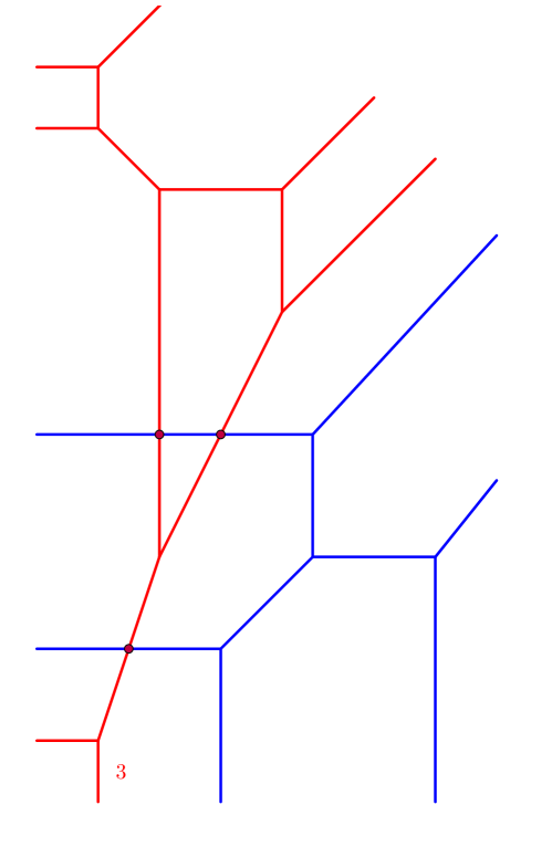
(a) A cubic curve and a conic curve.

(b) The dual subdivision of the union of the curves in (a).

Figure 4: Example of the dual subdivision.

Here, the polygon $\Delta_{1}+\Delta_{2}$ is the Minkowski sum of the polygons.

Bézout’s theorem for tropical curves is the following special instance. Assume that the degrees $\Delta_{1}=\Delta_{d_{1}}=\operatorname{Conv}(\{(0,0),(d_{1},0),(0,d_{1})\})$ and $\Delta_{2}=\Delta_{d_{2}}=\operatorname{Conv}(\{(0,0),(d_{2},0),(0,d_{2})\})$, i.e, the tropical curves $C_{1}$ and $C_{2}$ correspond to curves in the projective plane. Since

$$\Delta_{d_{1}}+\Delta_{d_{2}}=\operatorname{Conv}(\{(0,0),(d_{1}+d_{2},0),(0,d_{1}+d_{2})\})=\Delta_{d_{1}+d_{2}},$$

then we have that in this case

$$C_{1}\cdot C_{2}=\operatorname{Area}(\Delta_{d_{1}+d_{2}})-\operatorname{Area}(\Delta_{d_{1}})-\operatorname{Area}(\Delta_{d_{2}})=\frac{(d_{1}+d_{2})^{2}}{2}-\frac{d_{1}}{2}-\frac{d_{2}^{2}}{2}=d_{1}\cdot d_{2}.$$

3.4 Enriched tropical curves and Viro Polynomials

Viro’s patchworking is a combinatorial construction yielding topological properties of real algebraic curves. It is an algorithmic construction whose input is a subdivision of a polygon and a set of signs $\sigma(I)$ (either plus or minus) for every integer point $I$ in the dual subdivision of the polygon. A Viro polynomial associated to this data is a polynomial

$$\sum_{I\in\operatorname{DS}(\Delta)\cap\mathbb{Z}^{2}}\sigma(I)x^{i_{1}}y^{i_{2}}t^{\varphi(I)}$$

where $\varphi$ is a convex piece-wise linear function inducing the subdivision and such that tropicalizing the polynomial yields back a defining polynomial for the tropical curve. Based on this ideas, we generalize this concept by replacing the signs $\sigma(I)$ with elements $\alpha_{I}\in k^{\times}/(k^{\times})^{2}$ and call the following enriched Viro polynomial

$$\sum_{I\in\Delta\cap\mathbb{Z}^{2}}\alpha_{I}x^{i_{1}}y^{i_{2}}t^{\varphi(I)}.$$ (9)

Note that if $k=\mathbb{R}$, then this coincides with the original definition of a Viro polynomial since $\mathbb{R}^{\times}/(\mathbb{R}^{\times})^{2}=\{\pm 1\}$.

Tropicalization gives back a tropical curve $C$ which has the dual subdivision we started with. However, in the tropicalization process one loses information, namely the elements in $k^{\times}/(k^{\times})^{2}$. We would like to remember these coefficients by assigning them to the corresponding connected component in $\mathbb{R}^{2}\setminus C$, that is we assign the coefficient $\alpha_{I}$ of a monomial $x^{i_{1}}y^{i_{2}}t^{\varphi(I)}$ to the component where the $\nu(x^{i_{1}}y^{i_{2}}t^{\varphi(I)})=i_{1}\nu(x)+i_{2}\nu(y)-\varphi(I)$ attains the maximum. Equivalently, one can assign the coefficients $\alpha_{I}$ to the corresponding vertex $I$ in the dual subdivision. This gives rise to the following definition.

Definition 3.12.

An enriched tropical curve $\widetilde{C}=(C,(\alpha_{I}))$ over $k$ is a tropical curve $C$ with an element of $\alpha_{I}\in k^{\times}/(k^{\times})^{2}$ assigned to each connected component of $\mathbb{R}^{2}\setminus C$, or equivalently, to each vertex in the dual subdivision. We call such element $\alpha_{I}$ of $k^{\times}/(k^{\times})^{2}$ the coefficient of the component/vertex of the dual subdivision. We write $C$ for the underlying (classical) tropical curve.

To each enriched tropical curve $\widetilde{C}$ we can assign an (enriched) Viro polynomial of the form (9) such that tropicalizing and remembering the coefficients gives back $\widetilde{C}$.

Example 3.13.

Figure 5 shows an enriched tropical line and an enriched tropical conic with enriched Viro polynomials

$$\alpha_{(0,0)}+\alpha_{(1,0)}xt^{3}+\alpha_{(0,1)}yt^{3},$$

and respectively

$$\beta_{(0,0)}+\beta_{(1,0)}x+\beta_{(0,1)}y+\beta_{(2,0)}x^{2}t^{4}+\beta_{(1,1)}xyt^{2}+\beta_{(0,2)}y^{2}t^{4}.$$

Tropicalizing the enriched Viro polynomial of the line yields the tropical polynomial

$$``0+(-3)x+(-3)y"=\max\{0,x-3,y-3\}$$

which has tropical vanishing locus the tropical line with $3$-valent vertex at $(3,3)$ displayed in Figure 5. The enrichment remembers the coefficients of the enriched Viro polynomials and assigns them to the connected components where the tropicalization of the corresponding monomial attains the maximum.

Similarly, one can see that the tropicalization of the enriched Viro polynomial of the conic yields the tropical conic in Figure 5 as well as the coefficients of the connected components.

Definition 3.14.

Two enriched tropical curves $\widetilde{C}_{1}$ and $\widetilde{C}_{2}$ over $k$ intersect tropically transversally if the underlying tropical curves intersect tropically transversally and at every point $p$ in the intersection $C_{1}\cap C_{2}$, the intersection multiplicity $\operatorname{mult}_{p}(C_{1},C_{2})$ is not divisible by the characteristic of $k$.

(a) An enriched tropical line.

(b) An enriched tropical conic.

Figure 5: Examples of enriched tropical curves

In section 6 we want to quadratically enrich Theorem 3.11. In order to do this, we need to know the coefficients of the union $\widetilde{C}_{1}\cup\widetilde{C}_{2}$ of two enriched tropical curves $\widetilde{C}_{1}$ and $\widetilde{C}_{2}$. Let

$$f_{1}(x,y)=\sum_{I\in A}\alpha_{I}x^{i_{1}}y^{i_{2}}t^{\varphi(I)}\text{ and }f_{2}(x,y)=\sum_{J\in B}\beta_{J}x^{j_{1}}y^{j_{2}}t^{\psi(J)}$$ (10)

be enriched Viro polynomials of $\widetilde{C}_{1}$ and $\widetilde{C}_{2}$, respectively. Tropicalizing $f_{1}\cdot f_{2}$ yields the (non-enriched) tropical curve $C_{1}\cup C_{2}$. However the coefficients of the monomials of $f_{1}\cdot f_{2}$ are no longer elements of $k^{\times}$ but elements of $k\{\{t\}\}$. Recall from Example 2.7 that

$$k\{\{t\}\}^{\times}/(k\{\{t\}\}^{\times})^{2}\xrightarrow{\cong}k^{\times}/(k^{\times})^{2}\text{, }a=\sum_{i=m}^{\infty}a_{i}t^{i/N}\mapsto\operatorname{In}(a)=a_{m}$$

Hence, we want to find the initials of the coefficients of monomials of $f_{1}\cdot f_{2}$. It turns out that these initials are the product of coefficients of $\widetilde{C}_{1}$ and $\widetilde{C}_{2}$ where ”the intersection happens” (see Figure 6) as the following Lemma shows.

Lemma 3.15.

Let $\widetilde{C}_{1}$ and $\widetilde{C}_{2}$ be two enriched tropical curves with enriched Viro polynomials $f_{1}$ and $f_{2}$ as in (10). One can read of the coefficients of the enriched tropical curve $\widetilde{C}_{1}\cup\widetilde{C}_{2}$ as follows. Let $K=(k_{1},k_{2})\in\mathbb{Z}^{2}$ be a vertex of the dual subdivision of $C_{1}\cup C_{2}$. There are $I,J\in\mathbb{Z}^{2}$ such that $I$ is a vertex in the dual subdivision of $C_{1}$ and $J$ is a vertex in the dual subdivision of $C_{2}$, $K=I+J$ and such that the component dual to $K$ is a subset of the components dual to $I$ and $J$. Then the coefficient at the vertex $K$ of $\widetilde{C}_{1}\cup\widetilde{C}_{2}$ equals $\alpha_{I}\beta_{J}$.

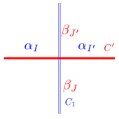
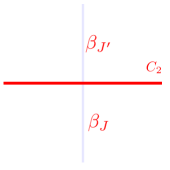
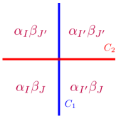
Figure 6: Coefficients of the union $\widetilde{C}_{1}\cup\widetilde{C}_{2}$ around an intersection point.

Proof.

We want to find the coefficients of the vertex $K$ in the dual subdivision of $\widetilde{C}_{1}\cup\widetilde{C}_{2}$. Let $(r,s)$ be a point in the interior of the component dual to $K$. Then $(r,s)$ is in the interior of the component in $\mathbb{R}^{2}\setminus C_{1}$ dual $I$ and in the interior of the component of $\mathbb{R}^{2}\setminus C_{2}$ dual to $J$. So $(r,s)$ is in the component where the tropicalizations of the monomials $\alpha_{I}x^{i_{1}}y^{i_{2}}t^{\varphi(I)}$ respectively $\beta_{J}x^{j_{1}}y^{j_{2}}t^{\psi(J)}$ are maximal. In other words,

$$i_{1}\cdot r+i_{2}\cdot s-\varphi(I)>i_{1}^{\prime}\cdot r+i_{2}^{\prime}\cdot s-\varphi(I^{\prime})$$

for any vertex $I^{\prime}\neq I$ in the dual subdivision of $C_{1}$ and

$$j_{1}\cdot r+j_{2}\cdot s-\psi(J)>j_{1}^{\prime}\cdot r+j_{2}^{\prime}\cdot s-\psi(J^{\prime})$$

for any vertex $J^{\prime}\neq J$ in the dual subdivision of $C_{2}$. Hence,

$$(i_{1}+j_{1})\cdot r+(i_{2}+j_{2})\cdot s-\varphi(I)-\psi(J)>(i_{1}^{\prime}+j_{1}^{\prime})\cdot r+(i_{2}^{\prime}+j_{2}^{\prime})\cdot s-\varphi(I^{\prime})-\psi(J^{\prime})$$

for any $(I^{\prime},J^{\prime})\neq(I,J)$. In particular for $(I^{\prime},J^{\prime})$ such that $I^{\prime}+J^{\prime}=I+J=K$ we get

$$\varphi(I)+\psi(J)<\varphi(I^{\prime})+\psi(J^{\prime}).$$

Hence, the monomial with exponent $K$ in $f_{1}\cdot f_{2}$ equals

$$\left(\alpha_{I}\beta_{J}t^{\varphi(I)+\psi(J)}+\text{higher order terms in }t\right)\cdot x^{k_{1}}y^{k_{2}}$$

and thus, the coefficient of $\widetilde{C}_{1}\cup\widetilde{C}_{2}$ at the vertex $K$ is $\alpha_{I}\beta_{J}$. ∎

3.5 Tropical hypersurfaces

Everything we did in this section, can also be generalized to other dimensions. Let $x=(x_{1},\ldots,x_{n})$ and

$$p(x)=``\sum_{I\in A}a_{I}x^{I}"\coloneqq``\sum_{I\in A}a_{I}x_{1}^{I_{1}}\cdots x_{n}^{I_{n}}"\in\mathbb{T}[x_{1},\ldots,x_{n}]$$ (11)

be a tropical polynomial in $n$ variables, i.e., $A$ is a finite set of tuples $I=(I_{1},\ldots,I_{n})\in\mathbb{Z}_{\geq 0}^{n}$ and $a_{I}\neq-\infty$ for $I\in A$.

Definition 3.16.

A tropical hypersurface in $\mathbb{R}^{n}$ is the tropical vanishing locus of a tropical polynomial in $n$ variables.

The tropical hypersurface defined by $p$ defined in (11) is of the form

$$V_{\operatorname{Trop}}(p)=\{(y_{1},\ldots,y_{n})\in\mathbb{R}^{n}\mid\exists I,I^{\prime}\in A:I\neq I^{\prime},p(y)=I\cdot\bar{y}+a_{I}=I^{\prime}\cdot\bar{y}+a_{I^{\prime}}\},$$

where $I\cdot\bar{y}=I_{1}y_{1}+\ldots+I_{n}y_{n}$ and $I^{\prime}\cdot\bar{y}=I_{1}^{\prime}y_{1}+\ldots+I_{n}^{\prime}y_{n}$.

Definition 3.17.

The Newton polytope of $V_{\operatorname{Trop}}(p)$ is the convex hull of the exponents of $p$ in $\mathbb{R}^{n}$,

$$\operatorname{NP}(p)\coloneqq\operatorname{Conv}(A).$$

As before we have a dual subdivision $\operatorname{DS}(p)$ of the Newton polytope $\operatorname{NP}(p)$. Just as in the case for curves, the connected components of $\mathbb{R}^{n}\setminus V_{\operatorname{Trop}}(p)$ correspond to vertices in $\operatorname{DS}(p)$ and the vertices of $V_{\operatorname{Trop}}(p)$ correspond to the maximal cells of $\operatorname{DS}(p)$.

We say that $n$ tropical hypersurfaces $V_{1},\ldots,V_{n}$ in $\mathbb{R}^{n}$ intersect tropically transversely at $p\in V_{1}\cap\ldots\cap V_{n}$ if the point $p$ belongs to the interior of a top dimensional face of $V_{i}$, for every $i=1,\dots,n$. In particular, for $n$ tropical hypersurfaces $V_{1},\ldots,V_{n}$ in $\mathbb{R}^{n}$ that intersect tropically transversely at $p\in V_{1}\cap\ldots\cap V_{n}$, i.e., the point $p$ corresponds to a parallelepiped in the dual subdivision of the union $V_{1}\cup\ldots\cup V_{n}$. Just as in the case for curves (8) one can identify the intersection multiplicity of $V_{1},\ldots,V_{n}$ at $p$ with the volume of the parallelepiped dual to $p$:

$$\operatorname{mult}_{p}(V_{1},\dots,V_{n})=\operatorname{\text{ Parallelepiped dual to }Vol}(p).$$

There is an analog of Theorem 3.11 in higher dimensions. Recall that the mixed volume $\operatorname{MVol}(\Delta_{1},\ldots,\Delta_{n})$ of $n$ polytopes in $\mathbb{R}^{n}$ is the coefficient of $\lambda_{1}\cdots\lambda_{n}$ in the polynomial $R(\lambda_{1},\ldots,\lambda_{n})$ given by $\operatorname{Vol}(\lambda_{1}\Delta_{1}+\ldots+\lambda_{n}\Delta_{n})$.

Theorem 3.18 (Tropical Bézout and Bernstein-Kushnirenko Theorem).

Let $V_{1},\ldots,V_{n}$ be tropical hypersurfaces in $\mathbb{R}^{n}$ with Newton polytopes $\Delta_{1},\ldots,\Delta_{n}$, respectively. Then

$$\sum_{p}\operatorname{mult}_{p}(V_{1},\ldots,V_{n})=\operatorname{MVol}(\Delta_{1},\ldots,\Delta_{n}).$$

In particular, if $\Delta_{i}=\Delta_{d_{i}}=d_{i}\cdot\Delta_{1}$ where $\Delta_{1}$ is the standard $n$-simplex for $i=1,\ldots,n$, then we get the tropical Bézout theorem

$$\sum_{p}\operatorname{mult}_{p}(V_{1},\ldots,V_{n})=d_{1}\cdots d_{n}.$$

3.5.1 Enriched tropical hypersurfaces

In section 6 we quadratically refine Theorem 3.18. Hence, we need to define enriched tropical hypersurfaces.

Definition 3.19.

An enriched tropical hypersurface $\widetilde{V}=(V,(\alpha_{I}))$ in $\mathbb{R}^{n}$ is a tropical hypersurface $V$ in $\mathbb{R}^{n}$ together with a coefficient $\alpha_{I}$ assigned to each connected component of $\mathbb{R}^{n}\setminus V$.

Just like in the case of curves, we can assign an enriched Viro polynomial

$$\sum_{I}\alpha_{I}x_{1}^{I_{1}}\dots x_{n}^{I_{n}}t^{\varphi(I)}$$ (12)

to an enriched tropical hypersurface $\widetilde{V}$ such that tropicalizing and remembering the coefficients yields back our enriched tropical hypersurface $\widetilde{V}$. Here, the sum is over a finite number of $n$-tuples $I\in\mathbb{Z}^{n}$, and $\varphi\colon\mathbb{Z}^{n}\rightarrow\mathbb{Q}$ is convex. The following is the higher dimensional analog of Lemma 3.15.

Lemma 3.20.

Let $\widetilde{V}_{1},\ldots,\widetilde{V}_{n}$ be $n$ enriched tropical hypersurfaces in $\mathbb{R}^{n}$ with enriched Viro polynomials

$$f_{i}(x)=\sum_{I^{i}\in A_{i}}x^{I^{i}}t^{\varphi_{i}(I^{i})}$$

for $i=1,\ldots,n$. Then one can read the coefficients of the enriched tropical hypersurface given by the union $\widetilde{V}_{1}\cup\widetilde{V}_{2}\cup\ldots\cup\widetilde{V}_{n}$ as follows. Let $K$ be a vertex in the dual subdivision of $\widetilde{V}_{1}\cup\widetilde{V}_{2}\cup\ldots\cup\widetilde{V}_{n}$. Let $J^{i}$ be the vertex in the dual subdivision of $\widetilde{V}_{i}$ such that the connected component dual to $K$ in $\mathbb{R}^{n}\setminus(\widetilde{V}_{1}\cup\ldots\widetilde{V}_{n})$ is a subset of the connected component in $\mathbb{R}^{n}\setminus\widetilde{V}_{i}$ dual to $J^{i}$ for each $i=1,\ldots,n$. Then the coefficient of the vertex $K$ of $\widetilde{V}_{1}\cup\widetilde{V}_{2}\cup\ldots\cup\widetilde{V}_{n}$ equals $\prod_{i=1}^{n}\alpha_{J^{i}}$.

Proof.

Let $p=(p_{1},\ldots,p_{n})$ be a point in the interior of the connected component in the complement $\mathbb{R}^{n}\setminus(\widetilde{V}_{1}\cup\ldots\cup\widetilde{V}_{n})$ that is dual to $K$. Then $p$ is in the interior of the connected component dual to $J^{i}$ in $\mathbb{R}^{n}\setminus\widetilde{V}_{i}$ for $i=1,\ldots,n$. That means that

$$\sum_{j=1}^{n}J^{i}_{j}\cdot p_{j}-\varphi_{i}(J^{i})>\sum_{j=1}^{n}I^{i}_{j}\cdot p_{j}-\varphi_{i}(I^{i})$$

for any $I^{i}\neq J^{i}$ and all $i=1,\ldots,n$. Hence,

$$\sum_{i=1}^{n}\left(\sum_{j=1}^{n}J^{i}_{j}\cdot p_{j}\right)-\sum_{i=1}^{n}\varphi_{i}(J^{i})>\sum_{i=1}^{n}\left(\sum_{j=1}^{n}I^{i}_{j}\cdot p_{j}\right)-\sum_{i=1}^{n}\varphi_{i}(I^{i})$$

for any $(I^{1},\ldots,I^{n})\neq(J^{1},\ldots,J^{n})$. In particular for $(I^{1},\ldots,I^{n})$ such that $\sum_{i=1}^{n}I^{i}=\sum_{i=1}^{n}J^{i}=K$ we get

$$\sum_{i=1}^{n}\varphi_{i}(J^{i})<\sum_{i=1}^{n}\varphi_{i}(I^{i})$$

and thus, the coefficient of $K$ equals $\prod_{i=1}^{n}\alpha_{J^{i}}$. ∎

4 Enriched tropical intersection multiplicity for curves

For expository reasons, we first prove our main theorem for tropical curves and do the general case in section 5. Throughout this section we will consider tropical curves enriched over a perfect field $k$ of characteristic not equal to $2$. However, our computations hold as long as the fields of definition of the intersection points are separable extensions of $k$.

Let $\widetilde{C}_{1}$ and $\widetilde{C}_{2}$ be two enriched tropical curves with enriched Viro polynomials

$$f_{1}=\sum_{I\in A}\alpha_{I}x^{i_{1}}y^{i_{2}}t^{\phi(I)}\text{ and }f_{2}=\sum_{J\in B}\beta_{I}x^{j_{1}}y^{j_{2}}t^{\psi(J)},$$

respectively, where both sums are over some finite subsets $A,B$ of $\mathbb{Z}^{2}$ and $\phi\colon A\rightarrow\mathbb{Z}$ and $\psi\colon B\rightarrow\mathbb{Z}$ are convex functions.

Definition 4.1.

We define the enriched intersection multiplicity of $\widetilde{C}_{1}$ and $\widetilde{C}_{2}$ at $p\in\widetilde{C}_{1}\cap\widetilde{C}_{2}$ to be

$$\widetilde{\operatorname{mult}}_{p}(\widetilde{C}_{1},\widetilde{C}_{2})\coloneqq\operatorname{Tr}_{E_{t}/k\{\{t\}\}}\left\langle\det\operatorname{Jac}(f_{1},f_{2})(z)\right\rangle\in\operatorname{GW}(k\{\{t\}\})$$

where $z$ is a solution to $f_{1}=f_{2}=0$ with $-\operatorname{val}(z)=p$ and $E_{t}$ is the coordinate ring of all such $z$.

Remark 4.2.

With the notation above, let $d_{1}=\deg f_{1}$ and $d_{2}=\deg f_{2}$ (in $x$ and $y$, not in $t$) and note that our definition of the enriched intersection multiplicity $\widetilde{\operatorname{mult}}_{p}(\widetilde{C}_{1},\widetilde{C}_{2})$ equals the local index (see Definition 2.21) of the section defined by $(f_{1},f_{2})$ of $\mathcal{O}_{\mathbb{P}^{2}_{k\{\{t\}\}}}(d_{1})\oplus\mathcal{O}_{\mathbb{P}^{2}_{k\{\{t\}\}}}(d_{2})$ at the zeros that tropicalize to $p$.

Assume that $\widetilde{C}_{1}$ and $\widetilde{C}_{2}$ intersect tropically transversally at $p$ and assume $z\in\bar{k}\{\{t\}\}^{2}$ tropicalizes to $p$. Then the maximum of $-\operatorname{val}(f_{1}(z))$ and $-\operatorname{val}(f_{2})(z)$ is attained exactly twice. This implies that the initial $z_{\circ}=(z_{1},z_{2})$ of $z$ has to satisfy binomial equations (by a binomial we mean a polynomial with two summands)

$$f_{1}^{\prime}=\alpha_{I}z_{1}^{i_{1}}z_{2}^{i_{2}}+\alpha_{I^{\prime}}z_{1}^{i_{1}^{\prime}}z_{2}^{i_{2}^{\prime}}=0$$

and

$$f_{2}^{\prime}=\beta_{J}z_{1}^{j_{1}}z_{2}^{j_{2}}+\beta_{J^{\prime}}z_{1}^{j_{1}^{\prime}}z_{2}^{j_{2}^{\prime}}=0.$$

These are exactly the summands of $f_{1}(x,y)$ and $f_{2}(x,y)$ for which the maximum of $-\operatorname{val}$ is attained. We call

$$f_{1}^{\prime}=\alpha_{I}x^{i_{1}}y^{i_{2}}+\alpha_{I^{\prime}}x^{i_{1}^{\prime}}y^{i_{2}^{\prime}}=0$$

and

$$f_{2}^{\prime}=\beta_{J}x^{j_{1}}y^{j_{2}}+\beta_{J^{\prime}}x^{j_{1}^{\prime}}y^{j_{2}^{\prime}}=0.$$

local binomial equations at $p$. In particular, we get that the coordinate ring of the initials of the points that tropicalize to $p$ equals

$$E\coloneqq\frac{k[x^{\pm 1},y^{\pm 1}]}{(f_{1}^{\prime},f_{2}^{\prime})}$$

where $f_{1}^{\prime},f_{2}^{\prime}\in k[x,y]$ are the local binomial equations at $p$.

Recall from Example 2.7 that $\operatorname{GW}(k)\cong\operatorname{GW}(k\{\{t\}\})$. The next theorem identifies the enriched intersection multiplicity $\widetilde{\operatorname{mult}}_{p}(\widetilde{C}_{1},\widetilde{C}_{2})\in\operatorname{GW}(k\{\{t\}\})$ with an element of $\operatorname{GW}(k)$ via this isomorphism.

Theorem 4.3.

Let $\widetilde{C}_{1}$ and $\widetilde{C}_{2}$ be enriched tropical curves in $\mathbb{R}^{2}$ with Newton polygons $\Delta_{1}$ and $\Delta_{2}$, respectively. If $\widetilde{C}_{1}$ and $\widetilde{C}_{2}$ intersect transversely at $p=(p_{1},p_{2})\in\mathbb{R}^{2}$, then the enriched intersection multiplicity $\widetilde{\operatorname{mult}}_{p}(\widetilde{C}_{1},\widetilde{C}_{2})$ at $p$ is given by

$$\operatorname{Tr}_{E/k}\left(\left\langle\det\left(\Delta I,\Delta J\right)\alpha_{I}\beta_{J}z_{\circ}^{I+J-e_{1}-e_{2}}\right\rangle\right)\in\operatorname{GW}(k)$$

where $\operatorname{Tr}$ is the trace map, $E$ the coordinate ring of all $z_{\circ}$ which are initials of solutions ${z\in\bar{k}\{\{t\}\}^{2}}$ with $-\operatorname{val}(z)=p$, $f_{1}^{\prime}=\alpha_{I}x^{i_{1}}y^{i_{2}}+\alpha_{I^{\prime}}x^{i_{1}^{\prime}}y^{i_{2}^{\prime}}$ and $f_{2}^{\prime}=\beta_{J}x^{j_{1}}y^{j_{2}}+\beta_{J^{\prime}}x^{j_{1}^{\prime}}y^{j_{2}^{\prime}}$ are the local binomial equation of $\widetilde{C}_{1}$ at $p$ and of $\widetilde{C}_{2}$ at $p$, respectively, and $\Delta I=I-I^{\prime}$, $\Delta J=J-J^{\prime}$.

Remark 4.4.

In particular, we see that if the two enriched tropical curves $\widetilde{C}_{1}$ and $\widetilde{C}_{2}$ intersect tropically transversally at $p$, then $\det\operatorname{Jac}(\widetilde{p})\neq 0$ and we can use (7).

Proof.

In order to compute the evaluation of the determinant of the Jacobian, let us remark that we have an isomorphism between the Grothendieck-Witt ring of the field of Puiseux series over $k$ and the Grothendieck-Witt ring of the field $k$ given by the initial map

$$\operatorname{In}\colon\begin{array}[]{ccc}\operatorname{GW}\left(k\{\{t\}\}\right)&\longrightarrow&\operatorname{GW}\left(k\right)\\ f(t)&\longmapsto&\operatorname{In}(f)\end{array}.$$

Hence, it suffices to compute the initial of the to the evaluation of the Jacobian of the equations defining the curves at the intersection point. Let $\widetilde{p}(t)\in\bar{k}\{\{t\}\}^{2}$ such that

$$\sum_{K\in\Delta_{1}\cap\Lambda}\alpha_{K}\widetilde{p}^{K}t^{\phi(K)}=\sum_{K\in\Delta_{2}\cap\Lambda}\beta_{K}\widetilde{p}^{K}t^{\varphi(K)}=0,$$

and such that $-val(\widetilde{p})=p$ and let $z_{\circ}=\operatorname{In}(\widetilde{p})$ be the initial of the lifting $\widetilde{p}$.

Since $\alpha_{I}z^{I}t^{\phi(I)}+\alpha_{I^{\prime}}z^{I^{\prime}}t^{\phi(I^{\prime})}$ is the local equation of $\widetilde{C}_{1}$ at $p$, and $\beta_{J}z^{J}t^{\varphi(J)}+\beta_{J^{\prime}}z^{J^{\prime}}t^{\varphi(J^{\prime})}$ is the local equation of $\widetilde{C}_{2}$ at $p$, the Jacobian of the intersection at $\widetilde{p}$ is given by the determinant

$$\begin{vmatrix}i_{1}\alpha_{I}z^{I-e_{1}}t^{\phi(I)}+i_{1}^{\prime}\alpha_{I^{\prime}}z^{I^{\prime}-e_{1}}t^{\phi(I^{\prime})}&i_{2}\alpha_{I}z^{I-e_{2}}t^{\phi(I)}+i_{2}^{\prime}\alpha_{I^{\prime}}z^{I^{\prime}-e_{2}}t^{\phi(I^{\prime})}\\ j_{1}\beta_{J}z^{J-e_{1}}t^{\varphi(J)}+j_{1}^{\prime}\beta_{J^{\prime}}z^{J^{\prime}-e_{1}}t^{\varphi(J^{\prime})}&j_{2}\beta_{J}z^{J-e_{2}}t^{\varphi(J)}+j_{2}^{\prime}\beta_{J^{\prime}}z^{J^{\prime}-e_{2}}t^{\varphi(J^{\prime})}\end{vmatrix},$$ (13)

evaluated at $\widetilde{p}$. To compute its initial we should first compute its valuation. We have that $\widetilde{p}$ satisfies

$$\alpha_{I}\widetilde{p}^{I}t^{\phi(I)}+\alpha_{I^{\prime}}\widetilde{p}^{I^{\prime}}t^{\phi(I^{\prime})}=0,\quad\beta_{J}\widetilde{p}^{J}t^{\varphi(J)}+\beta_{J^{\prime}}\widetilde{p}^{J^{\prime}}t^{\varphi(J^{\prime})}=0.$$ (14)

Then, we have that $\operatorname{val}\left(\alpha_{I}\widetilde{p}^{I}t^{\phi(I)}\right)=\operatorname{val}\left(\alpha_{I^{\prime}}\widetilde{p}^{I^{\prime}}t^{\phi(I^{\prime})}\right)$, and $\operatorname{val}\left(\beta_{J}\widetilde{p}^{J}t^{\varphi(J)}\right)=\operatorname{val}\left(\beta_{J^{\prime}}\widetilde{p}^{J^{\prime}}t^{\phi(J^{\prime})}\right)$. Equivalently,

$$-p_{1}i_{1}-p_{2}i_{2}+\phi(I)=-p_{1}i_{1}^{\prime}-p_{2}i_{2}^{\prime}+\phi(I^{\prime}),\text{ and }-p_{1}j_{1}-p_{2}j_{2}+\varphi(J)=-p_{1}j_{1}^{\prime}-p_{2}j_{2}^{\prime}+\phi(J^{\prime}),$$

where $I=(i_{1},i_{2})$, $I=(i_{1}^{\prime},i_{2}^{\prime})$, $J=(J_{1},J_{2})$, and $J^{\prime}=(J_{1}^{\prime},J_{2}^{\prime})$. This implies

$$\operatorname{val}(i_{1}\alpha_{I}\widetilde{p}^{I-e_{1}}t^{\phi(I)})=-p_{1}(i_{1}-1)-p_{2}i_{2}+\phi(I)=-p_{1}(i_{1}^{\prime}-1)-p_{2}i_{2}^{\prime}+\phi(I^{\prime})=\operatorname{val}(i_{1}^{\prime}\alpha_{I^{\prime}}\widetilde{p}^{I^{\prime}-e_{1}}t^{\phi(I^{\prime})}),$$

$$\operatorname{val}(i_{2}\alpha_{I}\widetilde{p}^{I-e_{2}}t^{\phi(I)})=-p_{1}i_{1}-p_{2}(i_{2}-1)+\phi(I)=-p_{1}i_{1}^{\prime}-p_{2}(i_{2}^{\prime}-1)+\phi(I^{\prime})=\operatorname{val}(i_{2}^{\prime}\alpha_{I^{\prime}}\widetilde{p}^{I^{\prime}-e_{2}}t^{\phi(I^{\prime})}),$$

$$\operatorname{val}(j_{1}\beta_{J}\widetilde{p}^{J-e_{1}}t^{\varphi(J)})=-p_{1}(j_{1}-1)-p_{2}j_{2}+\varphi(J)=-p_{1}(j_{1}^{\prime}-1)-p_{2}j_{2}^{\prime}+\varphi(J^{\prime})=\operatorname{val}(j_{1}^{\prime}\beta_{J^{\prime}}\widetilde{p}^{J^{\prime}-e_{1}}t^{\varphi(J^{\prime})}),$$

$$\operatorname{val}(j_{2}\beta_{J}\widetilde{p}^{J-e_{2}}t^{\varphi(J)})=-p_{1}j_{1}-p_{2}(j_{2}-1)+\varphi(J)=-p_{1}j_{1}^{\prime}-p_{2}(j_{2}^{\prime}-1)+\varphi(J^{\prime})=\operatorname{val}(j_{2}^{\prime}\beta_{J^{\prime}}\widetilde{p}^{J^{\prime}-e_{2}}t^{\varphi(J^{\prime})}).$$

Let us remark that, since the valuation of the product is the sum of the valuation of the factors, the valuation of the product of the entries in the diagonal is equal to the valuation of the product of the entries in the antidiagonal. Hence, the valuation of the determinant of the Jacobian (13) equals $-p_{1}(i_{1}-1)-p_{2}i_{2}+\phi(I)+-p_{1}j_{1}-p_{2}(j_{2}-1)+\varphi(J)$ given that the corresponding term does not vanish.

Let us start by computing the terms of every entry of degree corresponding to the calculated valuations. Using (14) the sum $i_{1}\alpha_{I}z^{I-e_{1}}t^{\phi(I)}+i_{1}^{\prime}\alpha_{I^{\prime}-e_{1}}z^{I^{\prime}}t^{\phi(I^{\prime})}$ evaluated at $\widetilde{p}$ equals

$$i_{1}\alpha_{I}\widetilde{p}^{I-e_{1}}t^{\phi(I)}+i_{1}^{\prime}\alpha_{I^{\prime}}\widetilde{p}^{I^{\prime}-e_{1}}t^{\phi(I^{\prime})} =i_{1}\alpha_{I}\widetilde{p}^{I-e_{1}}t^{\phi(I)}+i_{1}^{\prime}\widetilde{p}^{-e_{1}}\left(\alpha_{I^{\prime}}\widetilde{p}^{I^{\prime}}t^{\phi(I^{\prime})}\right)$$

$$=i_{1}\alpha_{I}\widetilde{p}^{I-e_{1}}t^{\phi(I)}+i_{1}^{\prime}\widetilde{p}^{-e_{1}}\left(-\alpha_{I}\widetilde{p}^{I}t^{\phi(I)}\right)$$

$$=\left(i_{1}-i_{1}^{\prime}\right)\left(\alpha_{I}\widetilde{p}^{I-e_{1}}t^{\phi(I)}\right),$$

whose term of degree $\operatorname{val}(i_{1}\alpha_{I}\widetilde{p}^{I-e_{1}}t^{\phi(I)})$ is $\left(i_{1}-i_{1}^{\prime}\right)\left(\alpha_{I}z_{\circ}^{I-e_{1}}\right)$. Similarly, the term of degree $\operatorname{val}(i_{2}\alpha_{I}\widetilde{p}^{I-e_{2}}t^{\phi(I)})$ of the sum $i_{2}\alpha_{I}z^{I-e_{2}}t^{\phi(I)}+i_{2}^{\prime}\alpha_{I^{\prime}}z^{I^{\prime}-e_{2}}t^{\phi(I^{\prime})}$ is $\left(i_{2}-i_{2}^{\prime}\right)\left(\alpha_{I}z_{\circ}^{I-e_{2}}\right)$; the term of degree $\operatorname{val}(j_{1}\beta_{J}\widetilde{p}^{J-e_{1}}t^{\varphi(J)})$ of the sum $j_{1}\beta_{J}z^{J-e_{1}}t^{\varphi(J)}+j_{1}^{\prime}\beta_{J^{\prime}}z^{J^{\prime}-e_{1}}t^{\varphi(J^{\prime})}$ is $\left(j_{1}-j_{1}^{\prime}\right)\left(\beta_{J}z_{\circ}^{J-e_{1}}\right)$; and lastly, the term of degree $\operatorname{val}(j_{2}\beta_{J}\widetilde{p}^{J-e_{2}}t^{\varphi(J)})$ of the sum $j_{2}\beta_{J}z^{J-e_{2}}t^{\varphi(J)}+j_{2}^{\prime}\beta_{J^{\prime}}z^{J^{\prime}-e_{2}}t^{\varphi(J^{\prime})}$ is  $\left(j_{2}-j_{2}^{\prime}\right)\left(\beta_{J}z_{\circ}^{J-e_{2}}\right)$. Therefore, the initial of the determinant of the Jacobian (13) is

$$\left[\left(i_{1}-i_{1}^{\prime}\right)\left(j_{2}-j_{2}^{\prime}\right)-\left(i_{2}-i_{2}^{\prime}\right)\left(j_{1}-j_{1}^{\prime}\right)\right]\left(\alpha_{I}\beta_{J}z_{\circ}^{I+J-e_{1}-e_{2}}\right),$$

which is non-zero since $\alpha_{I},\beta_{J},z_{\circ}\in k^{*}$, and the curves $C_{1}$ and $C_{2}$ intersect tropically transversally. ∎

Lemma 4.5.

If we exchange the roles of $I$ and $I^{\prime}$, or those of $J$ and $J^{\prime}$, the product

$$\det\left(\Delta I,\Delta J\right)\alpha_{I}\beta_{J}z_{\circ}^{I+J-e_{1}-e_{2}}$$

is invariant.

Proof.

This follows directly from equation (14). Indeed, the initial $z_{\circ}$ satisfies $\alpha_{I}z_{\circ}^{I}+\alpha_{I^{\prime}}z_{\circ}^{I^{\prime}}=0$. Hence, if we exchange the roles of $I$ and $I^{\prime}$ we have

$$\det((I^{\prime}-I),\Delta J)\alpha_{I^{\prime}}\beta_{J}z_{\circ}^{I^{\prime}+J-e_{1}-e_{2}} =\det((I^{\prime}-I),\Delta J)\left(\alpha_{I^{\prime}}z_{\circ}^{I^{\prime}}\right)\beta_{J}z_{\circ}^{J-e_{1}-e_{2}}$$

$$=\det((I^{\prime}-I),\Delta J)\left(-\alpha_{I}z_{\circ}^{I}\right)\beta_{J}z_{\circ}^{J-e_{1}-e_{2}}$$

$$=\det((I-I^{\prime}),\Delta J)\alpha_{I}\beta_{J}z_{\circ}^{I+J-e_{1}-e_{2}}.$$

The same argument proves the invariance with respect to the exchange of $J$ and $J^{\prime}$. ∎

4.1 A combinatorial formula for $\widetilde{\operatorname{mult}}_{p}(\widetilde{C}_{1},\widetilde{C}_{2})$

Recall that the intersections of two tropical curves $C_{1}$ and $C_{2}$ correspond to parallelograms in the dual subdivision of $C_{1}\cup C_{2}$ and that the classical tropical intersection multiplicity at an intersection point equals the area of this parallelogram, that means the interesection multiplicity can be read of the dual subdivision $\operatorname{DS}(C_{1}\cup C_{2})$ of $C_{1}\cup C_{2}$. Our goal is to find a way to determine the enriched intersection multiplicity with the help of the dual subdivision of two enriched tropical curves $\widetilde{C}_{1}$ and $\widetilde{C}_{2}$.

Each tropically transverse intersection point $p$ of $\widetilde{C}_{1}$ and $\widetilde{C}_{2}$ lies on an edge of $C_{1}$, respectively $C_{2}$, which separates two connected components of $\mathbb{R}^{2}\setminus C_{1}$, respectively of $\mathbb{R}^{2}\setminus C_{2}$. Each of these connected components has a coefficient assigned. Let us call these coefficients $\alpha_{I}$ and $\alpha_{I^{\prime}}$, respectively $\beta_{J}$ and $\beta_{J^{\prime}}$, as in Figure 6. Recall from Lemma 3.15 that the coefficients of the components of $\widetilde{C}_{1}\cup\widetilde{C}_{2}$ adjacent to intersection point $p$ are $\alpha_{I}\beta_{J}$, $\alpha_{I^{\prime}}\beta_{J}$, $\alpha_{I}\beta_{J^{\prime}}$ and $\alpha_{I^{\prime}}\beta_{J^{\prime}}$ as in figure 6. In particular, the vertices $I+J$, $I^{\prime}+J$, $I+J^{\prime}$ and $I^{\prime}+J^{\prime}$ of the parallelogram dual to $p$ in the dual subdivision of $\widetilde{C}_{1}\cup\widetilde{C}_{2}$ have coefficients $\alpha_{I}\beta_{J}$, $\alpha_{I^{\prime}}\beta_{J}$, $\alpha_{I}\beta_{J^{\prime}}$ and $\alpha_{I^{\prime}}\beta_{J^{\prime}}$, respectively.

Let $v$ be a corner vertex of a parallelogram $P$ in $\operatorname{DS}(\widetilde{C}_{1}\cup\widetilde{C}_{2})$ dual to a point $p\in\widetilde{C}_{1}\cap\widetilde{C}_{2}$. Set

$$\epsilon_{P}(v)\coloneqq\begin{cases}+1&\text{first $C_{1}$ then $C_{2}$}\\ -1&\text{first $C_{2}$ then $C_{1}$}\end{cases}$$ (15)

when walking around the vertex inside the parallelogram anticlockwise (see Figure 7) and note that this equals the sign of $\det(\pm\Delta I,\pm\Delta J)$, where each $\Delta I,\Delta J$ is oriented in a way that the vertices $v\pm\Delta I,v\pm\Delta J\in P$.

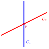
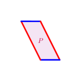
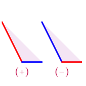
Figure 7: The dual parallelogram associated to an intersection point and a local picture of signed vertices.

Remark 4.6.

Note that the sign of the vertex $I+J$ is the same as the sign of $I^{\prime}+J^{\prime}$ and opposite of the sign of $I^{\prime}+J$ and $I+J^{\prime}$.

We are now ready to state our main theorem for in the case of curves. Recall that we say that a vertex $v\in\mathbb{Z}^{2}$ is odd if $v\equiv(1,1)$ in $(\mathbb{Z}/2\mathbb{Z})^{2}$.

Theorem 4.7.

Let $q$ be the number of odd corner vertices of the parallelogram $P$ dual to $p$ in the dual subdivision of $\widetilde{C}_{1}\cup\widetilde{C}_{2}$. Let $m$ be the classical intersection multiplicity at $p$ given by the area of the parallelogram $P$. Then,

$$\widetilde{\operatorname{mult}}_{p}(\widetilde{C}_{1},\widetilde{C}_{2})=\sum_{v\text{ odd}}\left\langle\epsilon_{P}(v)\alpha_{v}\right\rangle+\frac{m-q}{2}h\in\operatorname{GW}(k)$$

where the sum runs over all odd corners of $P$ and $\alpha_{v}=\alpha_{I}\beta_{J}$ is the coefficient of $v=I+J$.

Example 4.8.

Figure 8 shows the dual subdivision of the union of the tropical cubic and tropical conic in Figure 4. The parallelograms corresponding to the intersections are highlighted. Let $\alpha_{(3,1)}$ and $\alpha_{(1,3)}$ be the coefficients of the two odd vertices $(3,1)$ and $(1,3)$ of the dual subdivision. Then the intersection corresponding to the upper left parallelogram has enriched intersection multiplicity $\left\langle\alpha_{(1,3)}\right\rangle$, the one corresponding to the upper right parallelogram has enriched intersection multiplicity $\left\langle-\alpha_{(1,3)}\right\rangle+\left\langle-\alpha_{(3,1)}\right\rangle$ and the last one has enriched intersection multiplicity $h+\left\langle\alpha_{(3,1)}\right\rangle$.

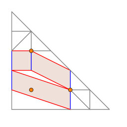
Figure 8: Odd vertices and their adjacent parallelograms in the dual subdivision of the curves in Figure 4.

4.2 Proof of Theorem 4.7

Recall that

$$E=\frac{k[x^{\pm 1},y^{\pm 1}]}{(f_{1}^{\prime},f_{2}^{\prime})}$$

with $f_{1}^{\prime}=\alpha_{I}x^{i_{1}}y^{i_{2}}+\alpha_{I^{\prime}}x^{i_{1}^{\prime}}y^{i_{2}^{\prime}}$ and $f_{2}^{\prime}=\beta_{J}x^{j_{1}}y^{j_{2}}+\beta_{J^{\prime}}x^{j_{1}^{\prime}}y^{j_{2}^{\prime}}$ the local binomial equations at $p$, is the coordinate ring of the initials of points that tropicalize to $p$. In Theorem 4.3 we computed the enriched intersection multiplicity of $\widetilde{C}_{1}$ and $\widetilde{C}_{2}$ at $p$ to be

$$\operatorname{Tr}_{E/k}\left\langle\det\left(\Delta I,\Delta J\right)\alpha_{I}\beta_{J}z_{\circ}^{I+J-e_{1}-e_{2}}\right\rangle\in\operatorname{GW}(k).$$

We use the notation

$$\Delta i_{1}=i_{1}-i_{1}^{\prime}\text{, }\Delta i_{2}=i_{2}-i_{2}^{\prime}\text{, }\Delta j_{1}=j_{1}-j_{1}^{\prime}\text{, }\Delta j_{2}=j_{2}-j_{2}^{\prime}.$$

In order to use our formulas for the trace in Proposition 2.13, we first show that $E$ is of the following form.

Proposition 4.9.

Let $m=\operatorname{mult}_{p}(C_{1},C_{2})$ be the classical intersection multiplicity of $C_{1}$ and $C_{2}$ at $p$. Then there is $d\in\mathbb{Z}_{\geq 1}$ such that $d$ divides $m$, and there are $D_{1}\in k$ and $D_{2}\in L\coloneqq\frac{k[w]}{(w^{\frac{m}{d}}-D_{1})}$ such that $E=\frac{L[w]}{(w^{d}-D_{2})}$.

Proof.

We aim to solve for $x$ and $y$ given the two equations

$$\alpha_{I}x^{i_{1}}y^{i_{2}}+\alpha_{I^{\prime}}x^{i_{1}^{\prime}}y^{i_{2}^{\prime}}=0\Leftrightarrow-\frac{\alpha_{I}}{\alpha_{I^{\prime}}}=x^{\Delta i_{1}}y^{\Delta i_{2}}$$ (16)

and

$$\beta_{J}x^{j_{1}}y^{j_{2}}+\beta_{J^{\prime}}x^{j_{1}^{\prime}}y^{j_{2}^{\prime}}=0\Leftrightarrow-\frac{\beta_{J}}{\beta_{J^{\prime}}}=x^{\Delta j_{1}}y^{\Delta j_{2}}.$$ (17)

We know that $\det\left(\Delta I,\Delta J\right)=\Delta i_{1}\Delta j_{2}-\Delta i_{2}\Delta j_{1}=\pm m$.

Let $d=\operatorname{gcd}(\Delta i_{1},\Delta j_{1})$. Then $\eqref{eq:alpha}^{-\frac{\Delta j_{1}}{d}}\cdot\eqref{eq:beta}^{\frac{\Delta i_{1}}{d}}$ yields

$$y^{\frac{m}{d}}=\left(-\frac{\alpha_{I^{\prime}}}{\alpha_{I}}\right)^{\frac{\Delta j_{1}}{d}}\cdot\left(-\frac{\beta_{J}}{\beta_{J^{\prime}}}\right)^{\frac{\Delta i_{1}}{d}}\eqqcolon D_{1}.$$

So $y\in L=\frac{k[w]}{(w^{\frac{m}{d}}-D_{1})}$. Since $\operatorname{gcd}(\frac{\Delta i_{1}}{d},\frac{\Delta j_{1}}{d})=1$ , there are $r,s\in\mathbb{Z}$ such that

$$r\cdot\frac{\Delta i_{1}}{d}+s\cdot\frac{\Delta j_{1}}{d}=1.$$

Now $\eqref{eq:alpha}^{r}\cdot\eqref{eq:beta}^{s}$ yields

$$x^{d}=y^{-\Delta i_{2}\cdot r-\Delta j_{2}\cdot s}\cdot\left(-\frac{\alpha_{I^{\prime}}}{\alpha_{I}}\right)^{r}\cdot\left(-\frac{\beta_{J^{\prime}}}{\beta_{J}}\right)^{s}\eqqcolon D_{2}$$

and thus $x\in\frac{L[w]}{(w^{d}-D_{2})}$.

∎

It follows that

$$\operatorname{Tr}_{E/k}\left(\left\langle\det(\Delta I,\Delta J)\alpha_{I}\beta_{J}z_{\circ}^{I+J-e_{1}-e_{2}}\right\rangle\right)=\operatorname{Tr}_{L/k}\circ\operatorname{Tr}_{E/L}\left(\left\langle\det(\Delta I,\Delta J)\alpha_{I}\beta_{J}z_{\circ}^{I+J-e_{1}-e_{2}}\right\rangle\right),$$

which we can compute with the help of Proposition 2.13.

Lemma 4.10.

The classical intersection multiplicity $m=\operatorname{mult}_{p}(C_{1},C_{2})$ is odd if and only if the parallelogram $P$ dual to $p$ has exactly one odd vertex.

Proof.

We first show that if $m$ is odd, then all four vertices of $P$ are pairwise different in ${(\mathbb{Z}/2\mathbb{Z})^{2}}$, and thus there is exactly one odd vertex. We know that $\Delta I\cdot\Delta J^{\bot}=\Delta i_{1}\cdot\Delta j_{2}-\Delta i_{2}\cdot\Delta j_{1}$ is odd. So one of the summands must be odd and the other even. Without loss of generality we can assume that both $\Delta i_{1}$ and $\Delta j_{2}$ are odd. Then at least one out of $\Delta i_{2}$ and $\Delta j_{1}$ is even. So there are three cases we need to check. In all the cases

$$\begin{pmatrix}0\\ 0\end{pmatrix},\begin{pmatrix}\Delta i_{1}\\ \Delta i_{2}\end{pmatrix},\begin{pmatrix}\Delta j_{1}\\ \Delta j_{2}\end{pmatrix},\begin{pmatrix}\Delta i_{1}+\Delta j_{1}\\ \Delta i_{2}+\Delta j_{2}\end{pmatrix}$$ (18)

are pairwise different in $(\mathbb{Z}/2\mathbb{Z})^{2}$. It follows that

$$I+J,I+J+\Delta I=I^{\prime}+J,I+J+\Delta J=I+J^{\prime},I+J+\Delta I+\Delta J=I^{\prime}+J^{\prime}$$

are pairwise different.

Now assume that there is exactly one odd vertex. This implies that the four vectors in (18) are pairwise different in $\mathbb{Z}/2\mathbb{Z}\times\mathbb{Z}/2\mathbb{Z}$. The area of this parallelogram is a non-zero element in $\mathbb{Z}/2\mathbb{Z}$, hence it is odd. ∎

Proof of Theorem 4.7.

(a) Intersection at $p$

(b) Dual parallelogram $P$

Figure 9: An enriched tropical intersection together with the dual parallelogram.

Recall from the proof of Proposition 4.9 that

$$D_{1}=\left(-\frac{\alpha_{I^{\prime}}}{\alpha_{I}}\right)^{\frac{\Delta j_{1}}{d}}\cdot\left(-\frac{\beta_{J}}{\beta_{J^{\prime}}}\right)^{\frac{\Delta i_{1}}{d}}$$ (19)

and

$$D_{2}=z_{2}^{-\Delta i_{2}\cdot r-\Delta j_{2}\cdot s}\cdot\left(-\frac{\alpha_{I}}{\alpha_{I^{\prime}}}\right)^{r}\cdot\left(-\frac{\beta_{J}}{\beta_{J^{\prime}}}\right)^{s},$$ (20)

where $r$ and $s$ are integers such that

$$r\cdot\frac{\Delta i_{1}}{d}+s\cdot\frac{\Delta j_{1}}{d}=1.$$ (21)

Furthermore, we set

$$D_{2}^{\prime}\coloneqq\left(-\frac{\alpha_{I}}{\alpha_{I^{\prime}}}\right)^{r}\cdot\left(-\frac{\beta_{J}}{\beta_{J^{\prime}}}\right)^{s}.$$ (22)

Recall that

$$m=|\Delta i_{1}\cdot\Delta j_{2}-\Delta i_{2}\cdot\Delta j_{1}|$$ (23)

equals the classical intersection multiplicity of $C_{1}$ and $C_{2}$ at $p$, and that

$$d=\gcd(\Delta i_{1},\Delta j_{1}).$$ (24)

Let $\epsilon\coloneqq\epsilon_{P}(I+J)$ be the sign of the vertex $I+J$ of $P$ and write $z_{\circ}=(z_{1},z_{2})\in\bar{k}^{2}$.

We prove the Theorem step by step going through all possible cases. We already know that the rank of the resulting form is $m=\operatorname{dim}_{k}E$. So we can compute everything in $\operatorname{W}(k)$, and then add hyperbolic summands to get an element of $\operatorname{GW}(k)$ of the correct rank.

$P$ has no odd vertex: First observe that $P$ has an odd vertex if $m$ is odd by Lemma 4.10, so we know that $m$ is even in this case.

1. If $d$ is odd, then at least one out of $\Delta i_{1}$ and $\Delta j_{1}$ must be odd and we can choose $I$ and $J$ such that $i_{1}+j_{1}-1$ is even by Lemma 4.5. In this case $i_{2}+j_{2}-1$ is odd otherwise there would be an odd vertex. Then

   $$\operatorname{Tr}_{E/L}\left(\left\langle\epsilon m\alpha_{I}\beta_{J}z_{\circ}^{I+J-e_{1}-e_{2}}\right\rangle\right)) =\operatorname{Tr}_{E/L}\left(\left\langle\epsilon m\alpha_{I}\beta_{J}z_{1}^{i_{1}+j_{1}-1}z_{2}^{i_{2}+j_{2}-1}\right\rangle\right)$$

   $$=\operatorname{Tr}_{E/L}\left(\left\langle\epsilon m\alpha_{I}\beta_{J}z_{2}\right\rangle\right)$$

   $$=\left\langle\epsilon md\alpha_{I}\beta_{J}z_{2}\right\rangle$$

   in $\operatorname{W}(L)$. Taking $\operatorname{Tr}_{L/k}$ we get $0\in\operatorname{W}(k)$ by Proposition 2.13 since $z_{2}\not\in k$ and $\frac{m}{d}$ must be even because $m$ is even.

2. If $d$ is even, then $\Delta i_{1}$ and $\Delta j_{1}$ are both even. So $i_{1}+j_{1}-1,i_{1}^{\prime}+j_{1}-1,i_{1}+j_{1}^{\prime}-1,i_{1}^{\prime}+j_{1}^{\prime}-1$ are either all even or all odd. If they are all odd, then

   $$\operatorname{Tr}_{E/L}\left(\left\langle\epsilon m\alpha_{I}\beta_{J}z_{\circ}^{I+J-e_{1}-e_{2}}\right\rangle\right)=\operatorname{Tr}_{E/L}\left(\left\langle\epsilon m\alpha_{I}\beta_{J}z_{2}^{i_{2}+j_{2}-1}z_{1}\right\rangle\right)=0$$

   in $\operatorname{W}(L)$ for any choice of $I$ and $J$ by Proposition 2.13 and our statement holds.

3. If $i_{1}+j_{1}-1,i_{1}^{\prime}+j_{1}-1,i_{1}+j_{1}^{\prime}-1,i_{1}^{\prime}+j_{1}^{\prime}-1$ are all even, then $i_{2}+j_{2}-1,{i_{2}^{\prime}+j_{2}-1},{i_{2}+j_{2}^{\prime}-1},$ ${i_{2}^{\prime}+j_{2}-1}$ must all be odd, otherwise there would be an odd vertex. This implies that $\Delta i_{2}$ and $\Delta j_{2}$ are both even and hence, both $d$ and $\frac{m}{d}$ are even. Thus

   $$\operatorname{Tr}_{E/L}\left(\left\langle\epsilon m\alpha_{I}\beta_{J}z_{\circ}^{I+J-e_{1}-e_{2}}\right\rangle\right)=\operatorname{Tr}_{E/L}\left(\left\langle\epsilon m\alpha_{I}\beta_{J}z_{2}\right\rangle\right)=\left\langle\epsilon md\alpha_{I}\beta_{J}z_{2}\right\rangle+\left\langle\epsilon md\alpha_{I}\beta_{J}D_{1}z_{2}\right\rangle$$

   and applying $\operatorname{Tr}_{L/k}$ we get $0\in\operatorname{W}(k)$ since $y\not\in k$.

$P$ has at least one odd vertex: we can assume that be $I+J$ is odd by Lemma 4.5. Then $\operatorname{Tr}_{E/k}\left\langle\epsilon\alpha_{I}\beta_{J}z_{\circ}^{I+J-e_{1}-e_{2}}\right\rangle=\operatorname{Tr}_{E/k}\left\langle\epsilon\alpha_{I}\beta_{J}\right\rangle$ is equal to

$d$ odd	$\frac{m}{d}$ odd	$\left\langle\epsilon\alpha_{I}\beta_{J}\right\rangle$
	$\frac{m}{d}$ even	$\left\langle\epsilon\alpha_{I}\beta_{J}\right\rangle+\left\langle\epsilon\alpha_{I}\beta_{J}D_{1}\right\rangle$
$d$ even	$\frac{m}{d}$ odd	$\Delta i_{2}\cdot r+\Delta j_{2}\cdot s$ odd	$\left\langle\epsilon\alpha_{I}\beta_{J}\right\rangle$+$\left\langle\epsilon\alpha_{I}\beta_{J}D_{2}^{\prime}D_{1}\right\rangle$
		$\Delta i_{2}\cdot r+\Delta j_{2}\cdot s$ even	$\left\langle\epsilon\alpha_{I}\beta_{J}\right\rangle$+$\left\langle\epsilon\alpha_{I}\beta_{J}D_{2}^{\prime}\right\rangle$
	$\frac{m}{d}$ even	$\Delta i_{2}\cdot r+\Delta j_{2}\cdot s$ odd	$\left\langle\epsilon\alpha_{I}\beta_{J}\right\rangle$+$\left\langle\epsilon\alpha_{I}\beta_{J}D_{1}\right\rangle$
		$\Delta i_{2}\cdot r+\Delta j_{2}\cdot s$ even	$\left\langle\epsilon\alpha_{I}\beta_{J}\right\rangle$+$\left\langle\epsilon\alpha_{I}\beta_{J}D_{1}\right\rangle$+$\left\langle\epsilon\alpha_{I}\beta_{J}D_{2}^{\prime}\right\rangle$+$\left\langle\epsilon\alpha_{I}\beta_{J}D_{2}^{\prime}D_{1}\right\rangle$

in $\operatorname{W}(k)$ by Proposition 2.13 and (19), (20) and (22).

By Lemma 4.10, our statement follows if $m$ is odd: For $m$ odd, both $d$ and $\frac{m}{d}$ must be odd. Thus we get

$$\widetilde{\operatorname{mult}}_{p}(C_{1},C_{2})=\left\langle\epsilon\alpha_{I}\beta_{J}\right\rangle+\frac{m-1}{2}h\in\operatorname{GW}(k)$$

where $I$ and $J$ are the unique choice such that $I+J=(1,1)$ in $\mathbb{Z}/2\mathbb{Z}\times\mathbb{Z}/2\mathbb{Z}$.

Assume $d$ is odd and $\frac{m}{d}$ is even: Since we assume $d=\gcd(\Delta i_{1},\Delta j_{1})$ to be odd, at least one out of $\Delta i_{1}$ and $\Delta j_{1}$ must be odd. Furthermore, we know that $\Delta i_{1}\cdot\Delta j_{2}\equiv\Delta i_{2}\cdot\Delta j_{2}\mod 2$ by (23). There are three possible cases.

1. $\Delta i_{1}\equiv\Delta j_{2}\equiv\Delta i_{2}\equiv\Delta j_{1}\equiv 1\mod 2$: Then $I+J$ and $I^{\prime}+J^{\prime}$ are odd and $I+J^{\prime}$ and $I^{\prime}+J$ are not. In this case, $\frac{\Delta i_{1}}{d}$ and $\frac{\Delta j_{1}}{d}$ are both odd, and thus

   $$\left\langle\epsilon\alpha_{I}\beta_{J}\right\rangle+\left\langle\epsilon\alpha_{I}\beta_{J}D_{1}\right\rangle=\left\langle\epsilon\alpha_{I}\beta_{J}\right\rangle+\left\langle\epsilon\alpha_{I^{\prime}}\beta_{J^{\prime}}\right\rangle.$$

2. $\Delta i_{1}\equiv 1\mod 2$ and $\Delta j_{2}\equiv\Delta j_{1}\equiv 0\mod 2$: Then $I+J$ and $I+J^{\prime}$ are odd while $I^{\prime}+J$ and $I^{\prime}+J^{\prime}$ are not. Then $\frac{\Delta i_{1}}{d}$ is odd and $\frac{\Delta j_{1}}{d}$ is even and

   $$\left\langle\epsilon\alpha_{I}\beta_{J}\right\rangle+\left\langle\epsilon\alpha_{I}\beta_{J}D_{1}\right\rangle=\left\langle\epsilon\alpha_{I}\beta_{J}\right\rangle+\left\langle-\epsilon\alpha_{I}\beta_{J^{\prime}}\right\rangle.$$

3. $\Delta j_{1}\equiv 1\mod 2$ and $\Delta i_{1}\equiv\Delta i_{2}\equiv 0\mod 2$: Then $I+J$ and $I^{\prime}+J$ are odd while $I+J^{\prime}$ and $I^{\prime}+J^{\prime}$ are not. Then $\frac{\Delta i_{1}}{d}$ is even and $\frac{\Delta j_{1}}{d}$ is odd and

   $$\left\langle\epsilon\alpha_{I}\beta_{J}\right\rangle+\left\langle\epsilon\alpha_{I}\beta_{J}D_{1}\right\rangle=\left\langle\epsilon\alpha_{I}\beta_{J}\right\rangle+\left\langle-\epsilon\alpha_{I^{\prime}}\beta_{J}\right\rangle.$$

$d$ is even and $\frac{m}{d}$ is odd: Since $d$ is even, both $\Delta i_{1}$ and $\Delta j_{1}$ are even and since $\frac{m}{d}$ equals $|\frac{\Delta i_{1}}{d}\cdot\Delta j_{2}-\frac{\Delta j_{1}}{d}\cdot\Delta i_{2}|$ and is odd, at least one out of $\Delta i_{2}$ and $\Delta j_{2}$ is odd.

1. If $\Delta i_{2}\equiv\Delta j_{2}\equiv 1\mod 2$, then $I+J$ and $I^{\prime}+J^{\prime}$ are odd, but $I+J^{\prime}$ and $I^{\prime}+J$ are not. Then $\Delta i_{2}\cdot r+\Delta j_{2}\cdot s\equiv r+s\mod 2$.

   1. If $r+s$ is odd, then either $r$ is odd and $s$ is even or the other way round. If $r$ is odd and $s$ is even, then $\frac{\Delta i_{1}}{d}$ must be odd because of (21). Furthermore, $\frac{\Delta j_{1}}{d}$ must be even, otherwise $\frac{m}{d}=|\frac{\Delta i_{1}}{d}\Delta j_{2}-\frac{\Delta j_{1}}{d}\Delta i_{2}|$ would be even. Thus, we get

      $$\left\langle\epsilon\alpha_{I}\beta_{J}\right\rangle+\left\langle\epsilon\alpha_{I}\beta_{J}D_{2}^{\prime}D_{1}\right\rangle=\left\langle\epsilon\alpha_{I}\beta_{J}\right\rangle+\left\langle\epsilon\alpha_{I^{\prime}}\beta_{J^{\prime}}\right\rangle.$$

      By the same argument, we get the same if $r$ is even and $s$ is odd.

   2. If $r+s$ is even, then both $r$ and $s$ must be odd since they cannot both be even because of (21). In this case we get

      $$\left\langle\epsilon\alpha_{I}\beta_{J}\right\rangle+\left\langle\epsilon\alpha_{I}\beta_{J}D_{2}^{\prime}\right\rangle=\left\langle\epsilon\alpha_{I}\beta_{J}\right\rangle+\left\langle\epsilon\alpha_{I^{\prime}}\beta_{J^{\prime}}\right\rangle.$$

2. If $\Delta i_{2}$ is odd and $\Delta j_{2}$ is even, then $I+J$ and $I+J^{\prime}$ are odd and $I^{\prime}+J$ and $I^{\prime}+J^{\prime}$ are not.

   1. If $r\cdot\Delta i_{2}+s\cdot\Delta j_{2}\equiv r\cdot\Delta i_{2}\equiv r\equiv 1\mod 2$, then also $\frac{\Delta j_{1}}{d}\equiv 1\mod 2$ since we have that $\frac{\Delta i_{1}}{d}\Delta j_{2}+\frac{\Delta j_{1}}{d}\Delta i_{2}\equiv\frac{m}{d}\equiv 1\mod 2$. Thus $r+\frac{\Delta j_{1}}{d}\equiv 0\mod 2$. Furthermore, in this case $s+\frac{\Delta i_{1}}{d}\equiv 1\mod 2$, since otherwise $\frac{\Delta i_{1}}{d}\cdot r+\frac{\Delta j_{1}}{d}\cdot s=1$ would be even. So we get in this case that

      $$\left\langle\epsilon\alpha_{I}\beta_{J}\right\rangle+\left\langle\epsilon\alpha_{I}\beta_{J}D_{1}D_{2}^{\prime}\right\rangle=\left\langle\epsilon\alpha_{I}\beta_{J}\right\rangle+\left\langle-\epsilon\alpha_{I}\beta_{J^{\prime}}\right\rangle.$$

   2. If $\Delta i_{2}\cdot r+\Delta j_{2}\cdot s\equiv 0\mod 2$ then $r$ must be even. Thus $s$ must be odd by (21) and we get

      $$\left\langle\epsilon\alpha_{I}\beta_{J}\right\rangle+\left\langle\epsilon\alpha_{I}\beta_{J}D_{2}^{\prime}\right\rangle=\left\langle\epsilon\alpha_{I}\beta_{J}\right\rangle+\left\langle-\epsilon\alpha_{I}\beta_{J^{\prime}}\right\rangle.$$

3. In case $\Delta i_{2}$ is even and $\Delta j_{2}$ is odd, we have that $I+J$ and $I^{\prime}+J$ are odd, and $I+J^{\prime}$ and $I^{\prime}+J^{\prime}$ are not and we get

   $$\left\langle\epsilon\alpha_{I}\beta_{J}\right\rangle+\left\langle-\epsilon\alpha_{I^{\prime}}\beta_{J}\right\rangle$$

   by the same argument as in the case above.

$d$ even and $\frac{m}{d}$ even:

1. If $\Delta i_{2}\cdot r+\Delta j_{2}\cdot s$ is odd, then at least one out of $\Delta i_{2}$ and $\Delta j_{2}$ must be odd.

   1. $\Delta i_{2}\equiv\Delta j_{2}\equiv 1\mod 2$: Then $\frac{\Delta j_{1}}{d}\equiv\frac{\Delta i_{1}}{d}\equiv 1\mod 2$ since $\frac{m}{d}$ is even and $\frac{\Delta j_{1}}{d}$ and $\frac{\Delta i_{1}}{d}$ cannot both be even since they are coprime. In this case, $I+J$ and $I^{\prime}+J^{\prime}$ are odd and $I+J^{\prime}$ and $I^{\prime}+J$ are not. We get

      $$\left\langle\epsilon\alpha_{I}\beta_{J}\right\rangle+\left\langle\epsilon\alpha_{I}\beta_{J}D_{1}\right\rangle=\left\langle\epsilon\alpha_{I}\beta_{J}\right\rangle+\left\langle\epsilon\alpha_{I^{\prime}}\beta_{J^{\prime}}\right\rangle.$$

   2. If $\Delta i_{2}$ is odd and $\Delta j_{2}$ is even, then $\frac{\Delta j_{1}}{d}$ is even, since $\frac{m}{d}$ is even. Then $\frac{\Delta i_{1}}{d}$ must be odd since $\gcd(\frac{\Delta i_{1}}{d},\frac{\Delta j_{1}}{d})=1$. So $I+J$ and $I+J^{\prime}$ are even while $I^{\prime}+J$ and $I^{\prime}+J^{\prime}$ are not. We get

      $$\left\langle\epsilon\alpha_{I}\beta_{J}\right\rangle+\left\langle\epsilon\alpha_{I}\beta_{J}D_{1}\right\rangle=\left\langle\epsilon\alpha_{I}\beta_{J}\right\rangle+\left\langle-\epsilon\alpha_{I}\beta_{J^{\prime}}\right\rangle.$$

   3. If $\Delta i_{2}$ is even and $\Delta j_{2}$ is odd, we know that $\frac{\Delta i_{1}}{d}$ is even and thus $\frac{\Delta j_{1}}{d}$ is odd by the same argument as in the case above. We get that $I+J$ and $I^{\prime}+J$ are odd while $I+J^{\prime}$ and $I^{\prime}+J^{\prime}$ are not and

      $$\left\langle\epsilon\alpha_{I}\beta_{J}\right\rangle+\left\langle\epsilon\alpha_{I}\beta_{J}D_{1}\right\rangle=\left\langle\epsilon\alpha_{I}\beta_{J}\right\rangle+\left\langle-\epsilon\alpha_{I^{\prime}}\beta_{J}\right\rangle.$$

2. If $\Delta i_{2}\cdot r+\Delta j_{2}\cdot s$ is even, then $\Delta i_{2}$ and $\Delta j_{2}$ must both be even:
   We know that $\frac{\Delta i_{1}}{d}\cdot r+\frac{\Delta j_{1}}{d}\cdot s=1$ and $\frac{\Delta i_{1}}{d}\cdot\Delta j_{2}\equiv\frac{\Delta j_{1}}{d}\cdot\Delta i_{2}\mod 2$ and one gets a contradiction to $\Delta i_{2}\cdot r+\Delta j_{2}\cdot s$ being even if one assumes that $\Delta i_{2}$ or $\Delta j_{2}$ is odd.
   So we get

   $$\left\langle\epsilon\alpha_{I}\beta_{J}\right\rangle+\left\langle\epsilon\alpha_{I}\beta_{J}D_{1}\right\rangle+\left\langle\epsilon\alpha_{I}\beta_{J}D_{2}^{\prime}\right\rangle+\left\langle\epsilon\alpha_{I}\beta_{J}D_{1}D_{2}^{\prime}\right\rangle$$

   $$= \left\langle\epsilon\alpha_{I}\beta_{J}\right\rangle+\left\langle-\epsilon\alpha_{I^{\prime}}\beta_{J}\right\rangle+\left\langle-\epsilon\alpha_{I}\beta_{J^{\prime}}\right\rangle+\left\langle\epsilon\alpha_{I^{\prime}}\beta_{J^{\prime}}\right\rangle.$$

∎

5 Higher Dimensions

We do an analog of the precedent section in higher dimensions. In this section we define the enriched intersection multiplicity $\widetilde{\operatorname{mult}}_{p}(V_{1},\dots,V_{n})$ of $n$ tropical hypersurfaces in $\mathbb{R}^{n}$ at an intersection point $p$ in terms of their defining polynomials. We prove that it can be computed by a purely combinatorial formula.

5.1 Notation

We start by establishing notation for the rest of the paper. This notation does not agree with the notation for curves, but both are natural notations for the cases they address. We use $\widetilde{V}$ for enriched tropical hypersurfaces. We write $V$ for the underlying (non-enriched) tropical hypersuface. Let $\widetilde{V}$ be an enriched tropical hypersurface in $\mathbb{R}^{n}$. Then we use the notation

$$\sum_{I\in A}\alpha_{I}x^{I}t^{\phi(I)}$$

for its enriched Viro equation. Here, the sum is over a finite set $A$ of $n$-tuples $I=(I_{1},\ldots,I_{n})\in\mathbb{Z}^{n}$, the map $\phi:A\rightarrow\mathbb{Q}$ the restriction of a rational convex function to $A$ and $x^{I}=x_{1}^{I_{1}}\cdots x_{n}^{I_{n}}$. The coefficients $\alpha_{I}$ are elements of $k^{\times}$. Now assume we have $n$ tropical hypersurfaces $\widetilde{V}_{1},\ldots,\widetilde{V}_{n}$ in $\mathbb{R}^{n}$ with enriched Viro equations

$$f_{i}=\sum_{I^{i}\in A_{i}}\alpha_{I^{i}}x^{I^{i}}t^{\phi_{i}(I^{i})}$$

for $i=1,\ldots,n$ and assume that $\widetilde{V}_{1},\ldots,\widetilde{V}_{n}$ intersect tropically transversally at $p$. Then for each $i\in\{1,\ldots,n\}$, the point $p$ lies on a top dimensional face of $\widetilde{V}_{i}$ separating two connected components of $\mathbb{R}^{n}$. Assume these components are the components where $I_{1}^{i}x_{1}+\ldots+I_{n}^{i}x_{n}-\phi_{i}(I^{i})$ and $J_{1}^{i}x_{1}+\ldots+J_{n}^{i}x_{n}-\phi_{i}(J^{i})$ attain the maximum for some $I^{i},J^{i}\in A_{i}$. Then we say that

$$f_{i}^{\prime}\coloneqq\alpha_{i}x^{I^{i}}+\beta_{i}x^{J^{i}}$$

is the local binomial equation of $\widetilde{V}_{i}$ at $p$. Put $\Delta^{i}\coloneqq I^{i}-J^{i}$ (the order of $I,J$ matters) and write $\det(\Delta^{i})$ for the determinant of the matrix with rows $\Delta^{1},\ldots,\Delta^{n}$. For an intersection point $p$ of $\widetilde{V}_{1},\ldots,\widetilde{V}_{n}$, we write $P$ for the parallelepiped in the dual subdivision of $\widetilde{V}_{1}\cup\ldots\cup\widetilde{V}_{n}$ dual to $p$. The parallelepiped $P$ is given by

$$P=\left\{\sum_{i=1}^{n}K^{i}\middle|K^{i}=I^{i}orJ^{i}\right\}.$$

For $z\in\macc@depth\char 1\relax\frozen@everymath{\macc@group}\macc@set@skewchar\macc@nested@a 111{k}\{\{t\}\}^{n}$ write $z_{\circ}\coloneqq(z_{1},\ldots,z_{n})=\operatorname{In}z\in\bar{k}^{n}$ for the initial of $z$. Furthermore, we let $e=(1,\ldots,1)\in\mathbb{Z}^{n}$ and $e_{i}=(0,\ldots,0,1,0,\ldots,0)$ with $1$ in the $i$th position. We set the vector $\hat{e}=(1,\ldots,1)\in\mathbb{Z}^{n-1}$ and write $\hat{x}=(x_{1},\ldots,x_{n-1})$. For $I\in\mathbb{Z}^{n}$, we put $\hat{I}\coloneqq(I_{1},\ldots,I_{n-1})\in\mathbb{Z}^{n-1}$.

5.2 Enriched tropical intersection multiplicity

We want to define the enriched intersection multiplicity to agree with the local index, as defined in Definition 2.21, at the zero of the section of $V\coloneqq\mathcal{O}(d_{1})\oplus\mathcal{O}(d_{2})\oplus\ldots\oplus\mathcal{O}(d_{n})\rightarrow\mathbb{P}^{n}_{k\{\{t\}\}}$ defined by the $n$ hypersurfaces in $\mathbb{P}^{n}_{k\{\{t\}\}}$. Assume our tropical hypersurfaces have enriched Viro equations $f_{1},\ldots,f_{n}\in k\{\{t\}\}[x_{1},\ldots,x_{n}]$. We have seen that the local index for the Poincaré-Hopf theorem for the vector bundle $V$ equals the local $\mathbb{A}^{1}$-degree of $(f_{1},\ldots,f_{n})\colon\mathbb{A}^{n}_{k\{\{t\}\}}\rightarrow\mathbb{A}^{n}_{k\{\{t\}\}}$ for which we have an explicit formula, namely the trace of the determinant of the Jacobian evaluated at the zero (see (7)). This motivates the following definition.

Definition 5.1.

Let $\widetilde{V}_{1},\ldots,\widetilde{V}_{n}$ be $n$ tropical hypersurfaces in $\mathbb{R}^{n}$ with defining polynomials $f_{1},\ldots,f_{n}\in k\{\{t\}\}[x_{1},\ldots,x_{n}]$. For an intersection point $p$, let $z$ be a closed point in $\mathbb{A}^{n}_{k\{\{t\}\}}$ such that $-\operatorname{val}(z)=p$ and such that $z$ is a zero of $f_{1}=\ldots=f_{n}=0$. We define the enriched intersection multiplicity of $\widetilde{V}_{1},\ldots,\widetilde{V}_{n}$ at $p$ to be

$$\widetilde{\operatorname{mult}}_{p}(\widetilde{V}_{1},\ldots,\widetilde{V}_{n})\coloneqq\operatorname{Tr}_{E_{t}/k\{\{t\}\}}\left\langle\det\operatorname{Jac}(f_{1},\ldots,f_{n})(z)\right\rangle\in\operatorname{GW}(k\{\{t\}\})$$ (25)

where $E_{t}$ is the coordinate ring of closed points in $\operatorname{Spec}k\{\{t\}\}[x_{1},\ldots,x_{n}]$ that are are zeros of $f_{1},\ldots,f_{n}$ with minus the valuation equal to $p$.

Recall that we write $z_{\circ}=(z_{1},\ldots,z_{n})$ for the closed point in $\mathbb{A}^{n}_{k}$ defined by the initials of $z$. Further, let $E$ be the coordinate ring of all $z_{\circ}$’s such that $z$ is a zero of $f_{1},\ldots,f_{n}$ and such that $-\operatorname{val}(z)=p=(p_{1},\ldots,p_{n})$. Let

$$f_{i}^{\prime}=\alpha_{i}z^{I^{i}}+\beta_{i}z^{J^{i}}$$ (26)

be the local binomial equation of $\widetilde{V}_{i}$ at $p$, for $i=1,\ldots,n$. The following Theorem is the $n$-dimensional analog of Theorem 4.3 for curves.

Theorem 5.2.

With the notation from Definition 25, if $\widetilde{V}_{1},\ldots,\widetilde{V}_{n}$ intersect tropically transversely at $p$, then

$$\left\langle\det\operatorname{Jac}(f_{1},\ldots,f_{n})(z)\right\rangle=\left\langle\det(\Delta^{i})\prod_{i=1}^{n}\alpha_{i}\cdot z_{\circ}^{\sum_{i=1}^{n}I^{i}-e}\right\rangle\in\operatorname{GW}(k\{\{t\}\})\cong\operatorname{GW}(k),$$

where $e=(1,1,\ldots,1)\in\mathbb{Z}^{n}$. In particular, the enriched intersection multiplicity at $p$ equals

$$\widetilde{\operatorname{mult}}_{p}(\widetilde{V}_{1},\ldots,\widetilde{V}_{n})=\operatorname{Tr}_{E/k}\left(\left\langle\det(\Delta^{i})\prod_{i=1}^{n}\alpha_{i}z_{\circ}^{\sum_{i=1}^{n}I^{i}-e}\right\rangle\right)\in\operatorname{GW}(k)$$

where $E$ is the coordinate ring of all such $z_{\circ}$.

Proof.

Just as in the proof of Theorem 4.3 it suffices to compute $\det\frac{\partial f_{i}^{\prime}}{\partial x_{j}}(z_{\circ})$. Using Equations 26 we have that

$$\det\frac{\partial f_{i}^{\prime}}{\partial x_{j}}(z_{\circ})_{i,j} =\det(I^{i}_{j}\alpha_{i}z_{\circ}^{I^{i}-e_{j}}+J^{i}_{j}\beta_{i}z_{\circ}^{J^{i}-e_{j}})_{i,j}$$

$$=\det(I^{i}_{j}\alpha_{i}z_{\circ}^{I^{i}-e_{j}}-J^{i}_{j}\alpha_{i}z_{\circ}^{I^{i}-e_{j}})_{i,j}$$

$$=\prod_{i=1}^{n}\alpha_{i}\cdot z_{\circ}^{\sum_{i=1}^{n}I^{i}-e}\cdot\det(I^{i}_{j}-J^{i}_{j})_{i,j}.$$

∎

The following Lemma shows that the enriched intersection multiplicity as calculated in Theorem 5.2 is independent of the choice of of the exponent vector $I^{j}$ or $J^{j}$, for $j=1,\ldots,n$.

Lemma 5.3.

The determinant of the Jacobian

$$\det\Delta^{i}\cdot\prod_{i=1}^{n}\alpha_{i}\cdot z_{\circ}^{\sum_{i=1}^{n}I^{i}-e}$$

is invariant under the exchange of the roles of $I^{j}$ and $J^{j}$ for any $j\in\{1,\ldots,n\}$.

Proof.

Recall that we have

$$f_{i}^{\prime}(z_{\circ})=\alpha_{i}z_{\circ}^{I^{i}}+\beta_{i}z_{\circ}^{J^{i}}=0$$

for $i=1,\ldots,n$, or equivalently,

$$-\frac{\beta_{i}}{\alpha_{i}}z_{\circ}^{J^{i}-I^{i}}=1.$$ (27)

If we exchange the roles of $I^{j}$ and $J^{j}$, we replace $\Delta^{j}=J^{j}-I^{j}$ by $-\Delta^{j}=I^{j}-J^{j}$ and then $\det\Delta^{i}\cdot\prod_{i=1}^{n}\alpha_{i}\cdot z_{\circ}^{\sum_{i=1}^{n}I^{n}-e}$ becomes

$$(-\det\Delta^{i})\cdot\prod_{\begin{subarray}{c}i=1\\ i\neq j\end{subarray}}^{n}\alpha_{i}\cdot\beta_{j}\cdot z_{\circ}^{\sum_{i=1}^{n}I^{i}-e+J^{j}-I^{j}}$$

$$= \left(-\frac{\beta_{j}}{\alpha_{j}}z_{\circ}^{J^{j}-I^{j}}\right)\cdot\det\Delta^{i}\cdot\prod_{i=1}^{n}\alpha_{i}\cdot z_{\circ}^{\sum_{i=1}^{n}I^{i}-e}$$

$$\overset{\eqref{eq:replaceIbyJ}}{=} \det\Delta^{i}\cdot\prod_{i=1}^{n}\alpha_{i}\cdot z_{\circ}^{\sum_{i=1}^{n}I^{i}-e}.$$

∎

5.3 A combinatorial formula for $\widetilde{\operatorname{mult}}_{p}(\widetilde{V}_{1},\ldots,\widetilde{V}_{n})$

Recall that an intersection of $n$ tropical hypersurfaces correspond to a parallelepiped in the dual subdivision of $V_{1}\cup\ldots\cup V_{n}$ and the volume of this parallelepiped equals the classical tropical intersection multiplicity. Theorem 5.2 assigns an enriched intersection multiplicity $\widetilde{\operatorname{mult}}_{p}(\widetilde{V}_{1},\ldots,\widetilde{V}_{n})$ to each intersection point $p$. We want to identify this enriched intersection multiplicity from Theorem 5.2 with an element of $\operatorname{GW}(k)$ which can be read of the dual subdivision of $\widetilde{V}_{1}\cup\ldots\cup\widetilde{V}_{n}$ just like in the case for curves. We will see that the intersection multiplicity we computed in Theorem 4.3 is determined by the odd vertices, in the sense of the following definition, in the dual subdivision of $\widetilde{V}_{1}\cup\ldots\cup\widetilde{V}_{n}$ in arbitrary dimension.

Definition 5.4.

We call a vertex $v=(v_{1},v_{2},\ldots,v_{n})\in\mathbb{Z}^{n}$ in the dual subdivision odd, if its class equals $(1,1,\ldots,1)$ in $(\mathbb{Z}/2\mathbb{Z})^{n}$.

Let $p$ be an intersection point of enriched tropical hypersurfaces $\widetilde{V}_{1},\ldots,\widetilde{V}_{n}$ and let $P$ be the parallelepiped in the dual subdivision of $\widetilde{V}_{1}\cup\ldots\cup\widetilde{V}_{n}$ dual to $p$. Let $q\in\{0,1,\ldots,2^{n}\}$ be the number of odd vertices $v_{1},\ldots,v_{q}$ of $P$. For $l=1,\ldots,q$ let $\alpha_{l}\coloneqq\prod_{i=1}^{n}\alpha^{(l)}_{I^{i}}$ be the coefficient of $v_{l}$. Furthermore, we assign a sign to the vertices $v_{1},\ldots,v_{q}$: Recall that locally at $p$ the Viro equations of $\widetilde{V}_{i}$ are of the form

$$f_{i}^{\prime}=\alpha_{i}x^{I^{i}}+\beta_{i}x^{J^{i}}$$

and

$$\Delta^{i}=I^{i}-J^{i}.$$

Let $v=\sum_{i=1}^{n}K^{i}$ be a vertex of $P$. Then the vertex $v$ can be expressed uniquely as

$$v=\sum_{i=1}^{n}I^{i}-\delta_{K^{i},J^{i}}\Delta^{i},$$

where $\delta_{K^{i},J^{i}}$ is the Kronecker delta. We define the sign of the vertex $v$ with respect to the parallelepiped $P$ as

$$\epsilon_{P}(v)\coloneqq\left(\prod_{i=1}^{n}(-1)^{\delta_{K^{i},J^{i}}}\right)\operatorname{sign}(\det\Delta^{i}).$$ (28)

Geometrically, the sign of the vertex $v$ with respect to the parallelepiped $P$ is the sign of the determinant of the edges of the parallelepiped $P$ adjacent to $v$ oriented outwards from $v$. Namely, if for every $i=1,\dots,n$ we put $\epsilon_{i}$ as the sign $\pm 1$ such that $v+\epsilon_{i}\Delta^{i}\in P$, then $\epsilon_{P}(v)=\operatorname{sign}(\det\epsilon_{i}\Delta^{i})$.

In particular, we have that

$$\epsilon_{P}(\sum_{i=1}^{n}I^{i})\cdot\operatorname{mult}_{p}(V_{1},\ldots,V_{n})=\det\Delta^{i},$$

and the sign, as defined here, agrees with the definition of the sign (15) for curves.

Remark 5.5.

Note that the sign of the vertex $\sum_{i=1}^{n}I^{i}$ is the opposite of the sign of $\sum_{i=1}^{n}I^{i}+J^{j}-I^{j}$ for any $j\in\{1,\ldots,n\}$. For example in the case of curves, we have that the sign of the vertex $I^{1}+I^{2}$ is the same as the sign of $J^{1}+J^{2}$ and opposite of the sign of $I^{1}+J^{2}$ and $J^{1}+I^{2}$ (compare with Remark 4.6).

Theorem 5.6 (Main theorem).

Let $p$ be an intersection point of enriched tropical hypersurfaces $\widetilde{V}_{1},\ldots,\widetilde{V}_{n}$ that intersect tropically transversally at $p$. Let $P$ be the parallelepiped corresponding to $p$ in the dual subdivision of $\widetilde{V}_{1},\ldots,\widetilde{V}_{n}$ corresponding to $p$ and let $v_{1},\ldots,v_{q}$ be the odd vertices of $P$. If the classical intersection multiplicity $\operatorname{mult}_{p}(V_{1},\ldots,V_{n})$ equals $m$, then

$$\widetilde{\operatorname{mult}}_{p}(\widetilde{V}_{1},\ldots,\widetilde{V}_{n})=\sum_{l=1}^{q}\left\langle\epsilon_{P}(v_{l})\alpha_{l}\right\rangle+\frac{m-q}{2}h\in\operatorname{GW}(k),$$

where $\alpha_{l}=\prod_{i=1}^{n}\alpha^{(l)}_{I^{i}}$ is the coefficient of the odd vertex $v_{l}$, for $l=1,\ldots,q$.

We are now ready to prove Theorem 5.6. Let

$$E=\frac{k[x_{1}^{\pm 1},\ldots,x_{n}^{\pm 1}]}{(\alpha_{i}x^{\Delta^{i}}+\beta_{i})_{i=1,\ldots,n}}.$$

Then $E$ is the coordinate ring of all initials $z_{\circ}$ of $z\in\bar{k}\{\{t\}\}^{n}$ such that $-\operatorname{val}(z)=p$.

Assume that $E$ is finite étale over $k$. Recall that we computed the intersection multiplicity of $\widetilde{V}_{1},\ldots,\widetilde{V}_{n}$ at $p$ to be

$$\operatorname{Tr}_{E/k}\left(\left\langle\det(\Delta^{i})\alpha_{v}z_{\circ}^{v-e}\right\rangle\right)\in\operatorname{GW}(k)$$

where $v=\sum_{i=1}^{n}I^{i}$ in Theorem 5.2. In order to use our formulas for the trace in Proposition 2.13, we first show that $E$ is of the following form.

Proposition 5.7.

Let $m=\operatorname{mult}_{p}(V_{1},\ldots,V_{n})$ be the classical intersection multiplicity of $V_{1},\ldots,V_{n}$ at $p$. Then there is a finite étale algebra $L$ over $k$ and $d\in\mathbb{Z}_{\geq 1}$ such that $d$ divides $m$ and $E=\frac{L[w^{\pm 1}]}{(w^{d}-D)}$ for some $D\in L$.

Proof.

The algebra $E$ is defined by the equations

$$\alpha_{i}x^{\Delta^{i}}+\beta_{i}\Leftrightarrow x^{\Delta^{i}}=-\frac{\beta_{i}}{\alpha_{i}}$$ (29)

for $i=1,\ldots,n$. Let $d=\gcd((\Delta^{1})_{n},(\Delta^{2})_{n},\dots,(\Delta^{n})_{n})$. Set $D\coloneqq x_{n}^{d}.$ Then the $n$ equations in $\eqref{eq:alphai}$ equal

$$\begin{split}\hat{x}^{\hat{\Delta}^{i}}\cdot D^{\frac{\Delta^{i}_{n}}{d}}=\left(-\frac{\beta_{i}}{\alpha_{i}}\right)\end{split}$$ (30)

for $i=1,\ldots,n$. Set

$$L\coloneqq\frac{k[x_{1}^{\pm 1},\ldots,x_{n-1}^{\pm 1},D^{\pm 1}]}{\left(\hat{x}^{\hat{\Delta}^{i}}\cdot D^{\frac{\Delta^{i}_{n}}{d}}+\frac{\beta_{i}}{\alpha_{i}}\right)_{i=1}^{n}}$$

and $d\coloneqq\operatorname{gcd}(\Delta_{n}^{1},\ldots,\Delta_{n}^{n})$. Pick integers $r_{1},\ldots,r_{n}$ such that $r_{1}\cdot(\Delta^{1})_{n}+\ldots+r_{n}\cdot(\Delta^{n})_{n}=d$. The product $\prod_{i=1}^{n}\eqref{eq:alphai}^{r_{i}}_{i}$ yields the equation

$$D=x_{n}^{d}=\hat{x}^{-\sum_{i=1}^{n}r_{i}\cdot\hat{\Delta}^{i}}\cdot\prod_{i=1}^{n}\left(-\frac{\beta_{i}}{\alpha_{i}}\right)^{r_{i}}\in L.$$ (31)

In particular, the map from $\frac{L[w^{\pm 1}]}{(w^{d}-D)}$ to $E$ determined by sending $w$ to $x_{n}$ is an isomorphism. ∎

Hence, we have a chain of field extensions $k<L<E$. It follows that

$$\operatorname{Tr}_{E/k}\left(\left\langle\det(\Delta^{i})\prod_{i=1}^{n}\alpha_{i}z_{\circ}^{\sum_{i=1}^{n}I^{i}-e}\right\rangle\right)=\operatorname{Tr}_{L/k}\circ\operatorname{Tr}_{E/L}\left(\left\langle\det(\Delta^{i})\prod_{i=1}^{n}\alpha_{i}z_{\circ}^{\sum_{i=1}^{n}I^{i}-e}\right\rangle\right)$$

which we can compute with the help of Proposition 2.13. Moreover, by defining

$$E^{i}\coloneqq\hat{\Delta}^{i}-\frac{\Delta^{i}_{n}}{d}\left(\sum_{j=1}^{n}r_{j}\hat{\Delta}^{j}\right),$$

we have that the equations (30) are equivalent to

$$\hat{x}^{E^{i}}=\left(\prod_{j=1}^{n}\left(-\frac{\beta_{j}}{\alpha_{j}}\right)^{r_{j}}\right)^{-\frac{\Delta^{i}_{n}}{d}}\left(-\frac{\beta_{i}}{\alpha_{i}}\right)$$ (32)

for $i=1,\dots,n$. These are equations in $n-1$ variables, defined over the field $k$. The determinant of the matrix formed by the vectors $\left(E^{i}\right)_{\begin{subarray}{c}i=1\\ i\neq j\end{subarray}}^{n}$ has determinant equal to $\pm r_{j}\frac{m}{d}$. Therefore, picking $j_{0}\in\{1,\dots,n\}$ such that $r_{j_{0}}\neq 0$, we have that the the equations (32) for $i=1,\dots,n,i\neq j_{0}$ are $n-1$ linearly independent equations in $n-1$ variables defining $L$ as a subalgebra of $E$. We will prove Theorem 5.6 by applying this reduction and using an inductive argument.

Proof of Theorem 5.6.

We prove the Theorem 5.6 by induction on $n$. Assume $n$ equals $1$. Then we have one equation

$$\alpha_{1}+\beta_{1}x^{\Delta^{1}}=0\Leftrightarrow x^{\Delta^{1}}=-\frac{\alpha_{1}}{\beta_{1}}\in k.$$

If $\Delta^{1}\in\mathbb{Z}^{1}=\mathbb{Z}$ is odd, then either $I^{1}$ or $J^{1}$ is odd. Assume $I^{1}$ is odd (if not change the roles of $I^{1}$ and $J^{1}$) and set $L=\frac{k[x^{\pm 1}]}{(\alpha_{1}+\beta_{1}x^{\Delta^{1}})}$. Note that $\epsilon(I^{1})\cdot m=\Delta$ and $\epsilon(I^{1})=\operatorname{sign}(I^{1})$ in case $n=1$. Then

$$\operatorname{Tr}_{L/k}\left(\left\langle\Delta^{1}\cdot\alpha_{1}z_{\circ}^{I^{1}-1}\right\rangle\right) =\operatorname{Tr}_{L/k}\left(\left\langle\Delta^{1}\cdot\alpha_{1}\right\rangle\right)$$

$$=\left\langle\epsilon(I^{1})\alpha_{1}\right\rangle+\frac{m-1}{2}h\in\operatorname{GW}(k)$$

by Proposition 2.13.

If $\Delta^{1}$ is even then either both $I^{1}$ and $J^{1}$ are even or both are odd. If both are even, then

$$\operatorname{Tr}_{L/k}\left(\left\langle\Delta^{1}\cdot\alpha_{1}z_{\circ}^{I^{1}-1}\right\rangle\right) =\operatorname{Tr}_{L/k}\left(\left\langle\Delta^{1}\cdot\alpha_{1}z_{\circ}\right\rangle\right)$$

$$=\frac{m}{2}h\in\operatorname{GW}(k)$$

by Proposition 2.13 since $z_{\circ}\not\in k$. If both $I^{1}$ and $J^{1}$ are odd, then

$$\operatorname{Tr}_{L/k}\left(\left\langle\Delta^{1}\cdot\alpha_{1}z_{\circ}^{I^{1}-1}\right\rangle\right) =\operatorname{Tr}_{L/k}\left(\left\langle\Delta^{1}\cdot\alpha_{1}\right\rangle\right)$$

$$=\left\langle\epsilon(I^{1})\alpha_{1}\right\rangle+\left\langle\epsilon(I^{1})\alpha_{1}\cdot(-\frac{\alpha_{1}}{\beta_{1}})\right\rangle+\frac{m-2}{2}h$$

$$=\left\langle\epsilon(I^{1})\alpha_{1}\right\rangle+\left\langle\epsilon(J^{1})\beta_{1}\right\rangle+\frac{m-2}{2}h\in\operatorname{GW}(k)$$

by Proposition 2.13.

Alternatively, we can use the case $n=2$ (Theorem 4.7) as our base for the induction.

Induction hypothesis: Assume we have an étale algebra $L$ over $k$ defined by $n-1$ linearly independent equations in $n-1$ variables with an isolated zero $\hat{z}_{\circ}$.

Further, assume that there exist a non-degenerated parallelepiped $P_{L}$ whose corners $\Lambda_{L}$ form a set of lattice points such that there exist coefficients $\alpha_{v}\in k^{\times}$, for $v\in\Lambda_{L}$, satisfying

$$\alpha_{v}\cdot\hat{z}_{\circ}^{v-\hat{e}}=\alpha_{w}\cdot\hat{z}_{\circ}^{w-\hat{e}}\in L^{\times}/(L^{\times})^{2}$$ (33)

for any $v,w\in\Lambda_{L}$. This implies that for any $v\in\Lambda_{L}$,

$$\operatorname{Tr}_{L/k}\left(\left\langle\operatorname{dim}_{k}L\cdot\alpha_{v}\cdot\hat{z}_{\circ}^{v-\hat{e}}\right\rangle\right)=\sum\left\langle\alpha_{v}\right\rangle\text{ in }\operatorname{W}(k),$$ (34)

where the sum runs over all lattice points $v\in\Lambda_{L}$ such that $v\equiv(1,\ldots,1)$ in $(\mathbb{Z}/2\mathbb{Z})^{n-1}$.

(a) $d$ odd, $\Delta^{2}_{3}$ even, $\Delta^{1}_{3}$ odd

(b) $d$ even, $I^{1}_{3}+I^{2}_{3}+I^{3}_{3}$ odd

Figure 10: Two examples of the reduction from a $3$-dimensional parallelepiped to the shaded ($2$-dimensional) parallelogram(s).

Induction step: Recall from Proposition 5.7 that $E=\frac{L[x]}{(x^{d}-D)}$ where $L$ is a finite étale algebra over $k$ and $d\in\mathbb{Z}_{\geq 1}$ divides $m$.

Recall also from the proof of Proposition 5.7 that $d=\gcd(\Delta_{n}^{i})_{i=1,\ldots,n}$. We also recall the following notation: $\hat{z}_{\circ}=(z_{1},\ldots,z_{n-1})$, $\hat{e}=(1,\ldots,1)\in\mathbb{Z}^{n-1}$ and ${\hat{I}^{i}=(I_{1}^{i},\ldots,I_{n-1}^{i})\in\mathbb{Z}^{n-1}}$. Further, recall that $\hat{z}_{\circ}$ is defined over $L$ and that $D=z_{n}^{d}\in L$.

Case 1: $d$ is odd. If $d$ is odd then we know that at least one of the $\Delta_{n}^{i}$ is odd. We can without loss of generality assume that $\Delta_{n}^{n}$ is odd. Then either $I^{n}_{n}$ or $J^{n}_{n}$ is odd (recall that $\Delta_{n}^{i}=I^{i}_{n}-J^{i}_{n}$). After possibly changing the roles of $I^{n}$ and $J^{n}$ which we can do by Lemma 5.3, we can assume that $\sum_{i=1}^{n}I^{i}_{n}$ is odd. Recall that $z_{i}\in L$ for $i=1,\ldots,n-1$ by the proof of Proposition 5.7. So we get

$$\operatorname{Tr}_{E/L}\left(\left\langle\det\Delta^{i}\prod_{i=1}^{n}\alpha_{i}z_{\circ}^{\sum_{i=1}^{n}I^{i}-e}\right\rangle\right) =\operatorname{Tr}_{E/L}\left(\left\langle\det\Delta^{i}\prod_{i=1}^{n}\alpha_{i}\hat{z}_{\circ}^{\sum_{i=1}^{n}\hat{I}^{i}-\hat{e}}z_{n}^{\sum_{i=1}^{n}I_{n}^{i}-1}\right\rangle\right)$$

$$=\operatorname{Tr}_{E/L}\left(\left\langle\det\Delta^{i}\prod_{i=1}^{n}\alpha_{i}\hat{z}_{\circ}^{\sum_{i=1}^{n}\hat{I}^{i}-\hat{e}}\right\rangle\right)$$

$$\overset{\ref{prop:traces}}{=}\left\langle\frac{\det\Delta^{i}}{d}\prod_{i=1}^{n}\alpha_{i}\hat{z}_{\circ}^{\sum_{i=1}^{n}\hat{I}^{i}-\hat{e}}\right\rangle\in\operatorname{W}(k)$$

by Proposition 2.13. Let $P_{L}$ be the convex hull of the set

$$\Lambda_{L}=\left\{\sum_{i=1}^{n}K^{i}_{n}\middle|K^{i}=I^{i}\text{ or }J^{i},\sum_{i=1}^{n}K^{i}_{n}\equiv 1\mod(2)\right\}.$$

In figure 10 (a) there is an example of the reduction from the $3$-dimensional parallelepiped $P$ to the shaded $2$-dimensional parallelepiped (shaded) $P_{L}$. In this example $\Delta_{3}^{1}$ and $\Delta_{3}^{3}$ (and thus also $d$) are odd, and $\Delta_{3}^{2}$ is even. The set $\Lambda_{L}$ has cardinality $2^{n-1}$ and the parallelepided $P_{L}$ can be seen as a transversal cut of the convex hull of $P=\left\{\sum_{i=1}^{n}{K}^{i}_{n}\middle|K^{i}=I^{i}\text{ or }J^{i}\right\}$, whose volume is $m$, hence $P_{L}$ is not degenerated. To use our induction hypothesis (34) we have to show that the set $\Lambda_{L}$ along with the coefficients

$$\alpha_{v}=\prod_{i=1}^{n}(\alpha_{i})^{\delta_{{K}^{i},{I}^{i}}}(-\beta_{i})^{\delta_{{K}^{i},{J}^{i}}},\text{ for }{v=\sum_{i=1}^{n}{K}^{i}}\in\Lambda_{L},$$ (35)

satisfy the equation (33). Put $v_{\circ}=\sum_{i=1}^{n}{I}^{i}\in\Lambda_{L}$. Then, we have that for any $v\in\Lambda_{L}$

$$\alpha_{v}\hat{z}_{\circ}^{\hat{v}-\hat{e}} =\alpha_{v}\cdot\hat{z}_{\circ}^{\sum_{i=1}^{n}\hat{K}^{i}-\hat{e}}$$

$$=\alpha_{v}\cdot z_{\circ}^{\sum_{i=1}^{n}K^{i}-e}\cdot z_{n}^{-(\sum_{i=1}^{n}K^{i}_{n}-1)}$$

$$=\alpha_{v}\cdot z_{\circ}^{\sum_{i=1}^{n}I^{i}-\delta_{{K}^{i},{J}^{i}}\cdot\Delta^{i}-e}\cdot z_{n}^{-(\sum_{i=1}^{n}I^{i}_{n}-\delta_{{K}^{i},{J}^{i}}\cdot\Delta^{i}_{n}-1)}$$

$$=\alpha_{v}\cdot\hat{z}_{\circ}^{\hat{v}_{\circ}-\hat{e}}\cdot z_{\circ}^{-\sum_{i=1}^{n}\delta_{{K}^{i},{J}^{i}}\cdot\Delta^{i}}\cdot z_{n}^{\sum_{i=1}^{n}\delta_{{K}^{i},{J}^{i}}\cdot\Delta^{i}_{n}}$$

$$=\prod_{i=1}^{n}(\alpha_{i})^{\delta_{{K}^{i},{I}^{i}}}(-\beta_{i})^{\delta_{{K}^{i},{J}^{i}}}\cdot\hat{z}_{\circ}^{\hat{v}_{\circ}-\hat{e}}\cdot\prod_{i=1}^{n}\left(-\frac{\beta_{i}}{\alpha_{i}}\right)^{-\delta_{{K}^{i},{J}^{i}}}\cdot z_{n}^{\sum_{i=1}^{n}\delta_{{K}^{i},{J}^{i}}\cdot\Delta^{i}_{n}}$$

$$=\prod_{i=1}^{n}(\alpha_{i})^{\delta_{{K}^{i},{I}^{i}}}(\alpha_{i})^{\delta_{{K}^{i},{J}^{i}}}\cdot\hat{z}_{\circ}^{\hat{v}_{\circ}-\hat{e}}\cdot z_{n}^{\sum_{i=1}^{n}\delta_{{K}^{i},{J}^{i}}\cdot\Delta^{i}_{n}}$$

$$=\alpha_{v_{\circ}}\cdot\hat{z}_{\circ}^{\hat{v}_{\circ}-\hat{e}}\cdot z_{n}^{\sum_{i=1}^{n}\delta_{{K}^{i},{J}^{i}}\cdot\Delta^{i}_{n}}.$$

Since $v,v_{\circ}\in\Lambda_{L}$, we have that $\sum_{i=1}^{n}\delta_{{K}^{i},{J}^{i}}\cdot\Delta^{i}_{n}=\sum_{i=1}^{n}I^{i}_{n}-\sum_{i=1}^{n}K^{i}_{n}\equiv 0\mod(2)$. Furthermore, since $\Delta^{i}_{n}\equiv 0\mod(d)$ and $d$ is odd, then $\sum_{i=1}^{n}\delta_{{K}^{i},{J}^{i}}\cdot\Delta^{i}_{n}\equiv 0\mod(2d)$ and

$$z_{n}^{\sum_{i=1}^{n}\delta_{{K}^{i},{J}^{i}}\cdot\Delta^{i}_{n}}=\left(D^{\frac{\sum_{i=1}^{n}\delta_{{K}^{i},{J}^{i}}\cdot\Delta^{i}_{n}}{2d}}\right)^{2}\in(L^{\times})^{2}.$$

By the induction hypothesis

$$\operatorname{Tr}_{L/k}\left\langle\frac{\det\Delta^{i}}{d}\prod_{i=1}^{n}\alpha_{i}\hat{z}_{\circ}^{\sum_{i=1}^{n}\hat{I}^{i}-\hat{e}}\right\rangle=\sum\left\langle\alpha_{v}\right\rangle\text{ in }\operatorname{W}(k),$$

where the sum runs over all $v\in\Lambda_{L}$ that are odd. Since every odd corner vertex of $P$ belongs to $\Lambda_{L}$, and for every $l\in\{1,\dots,q\}$ the coefficient $\alpha_{v_{l}}=\epsilon_{P}(v_{l})\cdot\alpha_{l}$, our statement follows.

Case 2: $d$ is even. This implies that $\Delta^{i}_{n}\equiv 0\mod(2)$, for all $i\in\{1,\dots,n\}$, and that $\sum_{i=1}^{n}K^{i}_{n}=\sum_{i=1}^{n}I^{i}_{n}-\delta_{{K}^{i},{J}^{i}}\Delta^{i}_{n}\equiv\sum_{i=1}^{n}I^{i}_{n}\mod(2)$.

If $\sum_{i=1}^{n}I^{i}_{n}\equiv 0\mod(2)$, then

$$\operatorname{Tr}_{E/L}\left\langle\det\Delta^{i}\prod_{i=1}^{n}\alpha_{i}z_{\circ}^{\sum_{i=1}^{n}I^{i}-e}\right\rangle =\operatorname{Tr}_{E/L}\left\langle\det\Delta^{i}\prod_{i=1}^{n}\alpha_{i}\hat{z}_{\circ}^{\sum_{i=1}^{n}\hat{I}^{i}-\hat{e}}z_{n}^{\sum_{i=1}^{n}I_{n}^{i}-1}\right\rangle$$

$$=\operatorname{Tr}_{E/L}\left\langle\det\Delta^{i}\prod_{i=1}^{n}\alpha_{i}\hat{z}_{\circ}^{\sum_{i=1}^{n}\hat{I}^{i}-\hat{e}}\cdot z_{n}\right\rangle$$

$$\overset{\ref{prop:traces}}{=}\frac{d}{2}h\in\operatorname{GW}(k),$$

which implies that

$$\operatorname{Tr}_{E/k}\left\langle\det\Delta^{i}\prod_{i=1}^{n}\alpha_{i}z_{\circ}^{\sum_{i=1}^{n}I^{i}-e}\right\rangle=0\in\operatorname{W}(k),$$

by Proposition 2.13. On the other hand, there are not odd vertices of $P$ since for every vertex the sum $\sum_{i=1}^{n}K^{i}_{n}\equiv\sum_{i=1}^{n}I^{i}_{n}\equiv 0\mod(2)$ and our statement follows.

Alternatively, if $\sum_{i=1}^{n}I^{i}_{n}\equiv 1\mod(2)$, then

$$\operatorname{Tr}_{E/L}\left\langle\det\Delta^{i}\prod_{i=1}^{n}\alpha_{i}z_{\circ}^{\sum_{i=1}^{n}I^{i}-e}\right\rangle =\operatorname{Tr}_{E/L}\left\langle\det\Delta^{i}\prod_{i=1}^{n}\alpha_{i}\hat{z}_{\circ}^{\sum_{i=1}^{n}\hat{I}^{i}-\hat{e}}z_{n}^{\sum_{i=1}^{n}I_{n}^{i}-e_{n}}\right\rangle$$

$$=\operatorname{Tr}_{E/L}\left\langle\det\Delta^{i}\prod_{i=1}^{n}\alpha_{i}\hat{z}_{\circ}^{\sum_{i=1}^{n}\hat{I}^{i}-\hat{e}}\right\rangle$$

$$\overset{\ref{prop:traces}}{=}\left\langle\det\Delta^{i}\prod_{i=1}^{n}\alpha_{i}\hat{z}_{\circ}^{\sum_{i=1}^{n}\hat{I}^{i}-\hat{e}}\right\rangle+\left\langle\det\Delta^{i}\prod_{i=1}^{n}\alpha_{i}\hat{z}_{\circ}^{\sum_{i=1}^{n}\hat{I}^{i}-\hat{e}}D\right\rangle,$$

in $\operatorname{W}(k)$. Let $P_{L_{0}}$ and $P_{L_{1}}$ be the convex hull of the sets

$$\Lambda_{L_{0}}=\left\{\sum_{i=1}^{n}{K}^{i}_{n}\middle|K^{i}=I^{i}\text{ or }J^{i},\sum_{i=1}^{n}\delta_{{K}^{i},{J}^{i}}\left(\frac{\Delta^{i}_{n}}{d}\right)\equiv 0\mod(2)\right\}\text{ and }$$

$$\Lambda_{L_{1}}=\left\{\sum_{i=1}^{n}{K}^{i}_{n}\middle|K^{i}=I^{i}\text{ or }J^{i},\sum_{i=1}^{n}\delta_{{K}^{i},{J}^{i}}\left(\frac{\Delta^{i}_{n}}{d}\right)\equiv 1\mod(2)\right\},$$

respectively. Figure 10 (b) shows an example of a parallelepiped $P$ and $P_{L_{0}}$ (the shaded parallelogram on the bottom) and $P_{L_{1}}$ (the shaded parallelogram on top). Each set of corners $\Lambda_{L_{i}}$ have $2^{n-1}$ elements and, analogously, each parallelepided $P_{L_{i}}$ can be seen as a transversal cut of $P$, whose volume is $m$, hence $P_{L_{i}}$ is not degenerated. To use our induction hypothesis (34) we have to show that each set $\Lambda_{L_{i}}$ along with the coefficients $\alpha_{v}$ defined as in (35) satisfy the equation (33). There exists an index $i_{0}\in\{1,\dots,n\}$ such that $\left(\frac{\Delta^{i_{0}}_{n}}{d}\right)\equiv 1\mod(2)$. Without loss of generality, assume that $i_{0}=n$. Put $v_{\circ}=\sum_{i=1}^{n}{I}^{i}\in\Lambda_{L_{0}}$ and $w_{\circ}=\sum_{i=1}^{n-1}\hat{I}^{i}+\hat{J}^{n}\in\Lambda_{L_{1}}$. An analogous computation as in the precedent case yields

$$\alpha_{v}\hat{z}_{\circ}^{\hat{v}-\hat{e}}=\alpha_{v_{\circ}}\cdot\hat{z}_{\circ}^{\hat{v}_{\circ}-\hat{e}}\cdot z_{n}^{\sum_{i=1}^{n}\delta_{{K}^{i},{J}^{i}}\cdot\Delta^{i}_{n}}=\alpha_{w_{\circ}}\cdot\hat{z}_{\circ}^{\hat{w}_{\circ}-\hat{e}}\cdot z_{n}^{\sum_{i=1}^{n}\delta_{{K}^{i},{J}^{i}}\cdot\Delta^{i}_{n}-\Delta^{n}_{n}}.$$

If $v\in\Lambda_{L_{0}}$, then

$$z_{n}^{\sum_{i=1}^{n}\delta_{{K}^{i},{J}^{i}}\cdot\Delta^{i}_{n}}=D^{\sum_{i=1}^{n}\delta_{{K}^{i},{J}^{i}}\cdot\frac{\Delta^{i}_{n}}{d}}\in(L^{\times})^{2}.$$

If $v\in\Lambda_{L_{1}}$, then

$$z_{n}^{\sum_{i=1}^{n}\delta_{{K}^{i},{J}^{i}}\cdot\Delta^{i}_{n}-\Delta^{n}_{n}}=D^{\sum_{i=1}^{n}\delta_{{K}^{i},{J}^{i}}\cdot\frac{\Delta^{i}_{n}}{d}-\frac{\Delta^{n}_{n}}{d}}\in(L^{\times})^{2}.$$

Furthermore, we have that

$$\alpha_{v_{\circ}}\cdot\hat{z}_{\circ}^{\hat{v}_{\circ}-\hat{e}}\cdot D=\alpha_{w_{\circ}}\cdot\hat{z}_{\circ}^{\hat{w}_{\circ}-\hat{e}}\cdot z_{n}^{-\Delta^{n}_{n}}\cdot D=\alpha_{w_{\circ}}\cdot\hat{z}_{\circ}^{\hat{w}_{\circ}-\hat{e}}\cdot D^{-\frac{\Delta^{n}_{n}}{d}+1}=\alpha_{w_{\circ}}\cdot\hat{z}_{\circ}^{\hat{w}_{\circ}-\hat{e}}\in L^{\times}/(L^{\times})^{2}.$$

Therefore,

$$\operatorname{Tr}_{E/k}\left\langle\det\Delta^{i}\prod_{i=1}^{n}\alpha_{i}z_{\circ}^{\sum_{i=1}^{n}I^{i}-e}\right\rangle =\operatorname{Tr}_{L/k}\left(\left\langle\det\Delta^{i}\alpha_{v_{\circ}}\hat{z}_{\circ}^{\hat{v}_{\circ}-\hat{e}}\right\rangle+\left\langle\det\Delta^{i}\alpha_{\hat{w}_{\circ}}\hat{z}_{\circ}^{w_{\circ}-\hat{e}}\right\rangle\right)$$

$$=\sum\left\langle\alpha_{v}\right\rangle\in\operatorname{W}(k)$$

where the sum runs over all lattice points $v\in\Lambda_{L_{0}}$ and $v\in\Lambda_{L_{1}}$ such that are odd. Those are exactly the odd vertices in $P$ since every vertex in $P$ has an odd $n$-th entry in this case.

∎

6 Enriched Tropical Bézout and Bernstein-Kushnirenko theorems

In sections 4 and 5 we assumed our algebras $E$ to be finite étale over the field $k$ in order to take the trace. Since we need this assumption for any point of intersection, we assume from now on that $k$ is a perfect field of characteristic not equal to $2$. We use properties of toric varieties to give applications of the computation we obtained in the precedent sections. For more details on toric varieties we refer to [Ful16] and [GKZ94].

6.1 A tropical proof of Bézout’s theorem enriched in $\operatorname{GW}(k)$

With the combinatorial formulas in Theorem 4.7 and in Theorem 5.6 for the enriched intersection multiplicity, we can quadratically enrich Bernd Sturmfels’ proof of the tropical Bézout theorem. The resulting count agrees with Stephen McKean’s nontropical Bézout’s theorem 2.23 in the relatively orientable case. In the non-relatively orientable case, we do not get an invariant result for the sum of enriched intersection multiplicities at the intersection points. However, our methods tell us all possible counts for this sum.

The proof of the enriched tropical Bézout theorem for curves is an easy corollary of the following Proposition.

Proposition 6.1.

Let $C_{1}$ and $C_{2}$ be tropical curves with Newton polygons $\Delta_{1}$ and $\Delta_{2}$, respectively. Let $v$ be a lattice point in the interior of $\Delta_{1}+\Delta_{2}$. Let

$$P_{v}\coloneqq\{\text{$P$ in $\operatorname{DS}(C_{1}\cup C_{2})$ dual to some $p\in C_{1}\cap C_{2}$, s.t. $v$ is a corner vertex of $P$}.\}$$

If the curves intersect tropically transversally, then

1. The cardinality $\operatorname{Card}(P_{v})$ is even.

2. There are equally many parallelograms $P$ in $P_{v}$ such that the sign $\epsilon(v)$ (as defined in (15)) in $P$ is positive as there are with negative sign

   $$\operatorname{Card}(\{P\in P_{v}\mid\epsilon_{P}(v)=+1\})=\operatorname{Card}(\{P\in P_{v}\mid\epsilon_{P}(v)=-1\}).$$

Proof.

Assume there are $N$ edges in the dual subdivision $\operatorname{DS}(C_{1}\cup C_{2})$ with vertex $v$. Each of these edges either corresponds to an edge of $C_{1}$ or an edge of $C_{2}$. We assign an element $i\in\mathbb{Z}/N\mathbb{Z}$ to each edge by walking around $v$ anticlockwise starting at some arbitrary edges with vertex $v$. Then the edges $i$ and $i+1$ correspond to different curves if and only if they are edges of a parallelogram corresponding to an intersection of $C_{1}$ and $C_{2}$. Since, $N+1=1$ in $\mathbb{Z}/N\mathbb{Z}$, there needs to be an even number of $i\in\mathbb{Z}/N\mathbb{Z}$ such that $i$ and $i+1$ correspond to different curves. Hence, there is an even number of parallelograms with vertex $v$ which correspond to an intersection of $C_{1}$ and $C_{2}$. Furthermore, the number of $i$ where $i$ corresponds to an edge in $C_{1}$ and $i+1$ corresponds to an edge in $C_{2}$ must be equal to the number of $i$ where $i$ corresponds to an edge in $C_{2}$ and $i+1$ corresponds to an edge in $C_{1}$. Now note that the first case corresponds to an intersection with positive sign and the latter to an intersection with negative sign (see (15)). ∎

Example 6.2.

In Figure 8 there are three odd points in the interior of the Newton polygon. The points $(3,1)$ and $(1,3)$ are both vertices of two parallelograms corresponding to intersection points, while $(1,1)$ is not a vertex of a parallelogram. Summing up the intersection multiplicities found in Example 4.8 we get $3h$ which coincides with Stephen McKean’s enriched (non-tropical) Bézout Theorem 2.23.

Let

$$\Delta_{d}=\operatorname{Conv}\{(0,0),(d,0),(0,d)\}\subset\mathbb{R}^{2}$$

be the Newton polygon of a general degree $d$ polynomial in $2$ variables. Note that if $C_{1}$ and $C_{2}$ are tropical curves with Newton polygons $\Delta_{d_{1}}$ and $\Delta_{d_{2}}$ than $C_{1}\cup C_{2}$ has Newton polygon $\Delta_{d_{1}+d_{2}}$.

Corollary 6.3 (Enriched tropical Bézout for curves).

Let $\widetilde{C}_{1}$ and $\widetilde{C}_{2}$ be two enriched tropical curves with Newton polygons $\Delta_{d_{1}}$ and $\Delta_{d_{2}}$, respectively, such that $d_{1}+d_{2}\equiv 1\mod 2$. Further, assume that $\widetilde{C}_{1}$ and $\widetilde{C}_{2}$ intersect tropically transversely at every intersection point $p\in\widetilde{C}_{1}\cap\widetilde{C}_{2}$. Then

$$\sum_{p\in\widetilde{C}_{1}\cap\widetilde{C}_{2}}\widetilde{\operatorname{mult}}_{p}(\widetilde{C}_{1},\widetilde{C}_{2})=\frac{d_{1}\cdot d_{2}}{2}h\in\operatorname{GW}(k).$$

Proof.

For $v$ in the interior of $\Delta_{d_{1}+d_{2}}$ let $N(v)$ be the number of parallelograms in the dual subdivision of $\widetilde{C}_{1}\cup\widetilde{C}_{2}$ which correspond to an intersection of $\widetilde{C}_{1}$ and $\widetilde{C}_{2}$. Call the coefficient of $v$ in $\operatorname{DS(\widetilde{C}_{1}\cup\widetilde{C}_{2})}$ $\alpha_{v}$. By Theorem 4.7 and Proposition 6.1 we have

$$\sum_{p}\widetilde{\operatorname{mult}}_{p}(\widetilde{C}_{1},\widetilde{C}_{2})=\sum_{v}\left(\frac{N(v)}{2}\left\langle\alpha_{v}\right\rangle+\frac{N(v)}{2}\left\langle-\alpha_{v}\right\rangle\right)\text{ in }\operatorname{W}(k)$$

where the first sum runs over the intersection points of $\widetilde{C}_{1}$ and $\widetilde{C}_{2}$ and the second sum runs over the odd vertices in the interior of $\Delta_{d_{1}+d_{2}}$. Since $\left\langle a\right\rangle+\left\langle-a\right\rangle=0$ in $\operatorname{W}(k)$, we get that $\sum_{v}\left(\frac{n(v)}{2}\left\langle\alpha_{v}\right\rangle+\frac{n(v)}{2}\left\langle-\alpha_{v}\right\rangle\right)=0$ in $\operatorname{W}(k)$ and thus $\sum_{p}\widetilde{\operatorname{mult}}_{p}(\widetilde{C}_{1},\widetilde{C}_{2})$ equals a multiple of $h$ in $\operatorname{GW}(k)$. By Example 2.5 the classical tropical Bézout theorem tells us the rank of the sum $\sum_{p}\widetilde{\operatorname{mult}}_{p}(\widetilde{C}_{1},\widetilde{C}_{2})$, which equals $\sum_{p}\operatorname{mult}_{p}(C_{1},C_{2})=d_{1}\cdot d_{2}$. Recall that an element of $\operatorname{GW}(k)$ is determined by its rank and its image in the Witt group $\operatorname{W}(k)$ (see Remark 2.9). Thus we get

$$\sum_{p}\widetilde{\operatorname{mult}}_{p}(\widetilde{C}_{1},\widetilde{C}_{2})=\frac{d_{1}\cdot d_{2}}{2}\cdot h\text{ in }\operatorname{GW}(k).$$

∎

We can generalize the proof of Proposition 6.1 to higher dimensions.

Proposition 6.4.

Let $V_{1},\ldots,V_{n}$ be $n$ tropical hypersurfaces in $\mathbb{R}^{n}$ with associated Newton polytopes $\Delta_{1},\ldots,\Delta_{n}$, respectively. Let $v$ be an odd lattice point in the interior of $\Delta_{1}+\ldots+\Delta_{n}$ and let

$$P_{v}\coloneqq\{\text{$P$ in $\operatorname{DS}(V_{1}\cup\ldots\cup V_{n})$ dual to some $p\in V_{1}\cap\ldots\cap V_{n}$, s.t. $v$ is a corner vertex of $P$}\}.$$

If the hypersurfaces $V_{1},\ldots,V_{n}$ intersect tropically transversely, then

1. The cardinality $\operatorname{Card}(P_{v})$ of $P_{v}$ is even.

2. There are equally many parallelepipeds $P$ in $P_{v}$ such that the sign $\epsilon_{P}(v)$ (as defined in (28)) in $P$ is positive as there are with negative sign

   $$\operatorname{Card}(\{P\in P_{v}\mid\epsilon_{P}(v)=+1\})=\operatorname{Card}(\{P\in P_{v}\mid\epsilon_{P}(v)=-1\}).$$

Proof.

Due to the transversality hypothesis, the hypersurfaces $V_{1},\ldots,V_{n-1}$ intersect along a tropical curve $C\subset\mathbb{R}^{n}$. This curve intersects $V_{n}$ tropically transversely. Let us denote by $R_{v}\subset\mathbb{R}^{n}$ the region where the monomial of exponent $v$ is maximal in the product of defining equations of the hypersurfaces $V_{1},\ldots,V_{n}$. Since $v$ is an inner lattice point of the dual polytope, the region $R_{v}$ is a bounded polytope. If $P_{v}$ is empty, our assertion follows. Otherwise, let $p\in C\cap V_{n}$ be an intersection point such that its dual polytope $P\in P_{v}$. Let $\gamma$ be the connected component of $C\cap\partial R_{v}$ containing the point $p$. We claim that $\gamma$ is a piece-wise linear path. Namely, the set $\gamma$ is formed by two segments of edges of $C$ containing intersection points with $V_{n}$, together with bounded edges. If a vertex $w$ of $C$ is in $\gamma$, its valency in $\gamma$ is $2$, corresponding to the edges in $C$ adjacent to the region where the monomial corresponding to $R_{v}$ is maximal. Since $R_{v}$ is a bounded polytope, the curve $\gamma$ is compact, having an endpoint $q$ that is in $V_{n}$. Indeed, the point $q\neq p$ cannot be a vertex of $C$, or its valency in $\gamma$ would be $1$, hence it is an inner point of an edge of $C$. Since there are no changes in the monomials where the maximum is achieved in the interior of an edge, this change is produced by the hypersurface $V_{n}$. Therefore, these paths $\gamma$ establish a pairing between the intersection points of $C\cap V_{n}$ adjacent to $R_{v}$.

We transfer the frame in $p$ through $\gamma$ to show that the polytopes corresponding to the endpoints of $\gamma$ have opposite sign at the vertex $V$. For that, let us start by recalling that the sign $\epsilon_{P}(v)$ is the sign of the determinant $\left(\Delta^{i}\right)_{i=1}^{n}$, where every $\Delta^{i}$ has been oriented in such a way that ${v+\Delta^{i}\in P}$. This oriented vector is the normal vector of the facet of $V_{i}$ pointing outwards to the region $R_{v}$. Let us define $w_{p}\coloneqq\bigwedge_{i=1}^{n-1}\Delta^{i}$ (the vector of alternating minors of the $n-1\times n$ matrix $\left(\pm\Delta^{i}\right)_{i=1}^{n-1}$). The vector $w_{p}$ is a director vector of the edge of $C$ containing $p$, albeit not a primitive one. Moreover, the sign $\epsilon_{P}(V)=\operatorname{sign}(\det\left(\Delta^{i}\right)_{i=1}^{n})=\operatorname{sign}(w_{p}\cdot\Delta^{n})$ can be computed as the sign of the inner product of $w_{p}$ with the normal vector of the facet of $V_{n}$ containing $p$, oriented outwards the region $R_{v}$. We can define $w_{\gamma(t)}$ for every point of $\gamma$ that is an inner point of an edge of $C$. If we oriented $\gamma$ as a path starting at $p$, at every point $\gamma(t)$, the orientations of $w_{\gamma(t)}$ and $\gamma$ would have the same relation (either coincide or differ), since the relative position of the normal vectors of the facets of $V^{i}$ at $\gamma(t)$ does not change in the boundary of $R_{v}$. This implies that exactly one of the vectors $w_{p}$ at $p\in V_{n}$ or $w_{q}$ at $q\in V_{n}$ is oriented towards the region $R_{v}$ while the other one is not. Hence, the endpoints of $\gamma$ have opposite signs. ∎

As a corollary we get an enriched tropical Bézout theorem. For this let

$$\Delta_{d}=\operatorname{Conv}\{(0,0,\ldots,0),(d,0,\ldots,0),(0,d,0,\ldots,0),\ldots,(0,\ldots,0,d)\}\subset\mathbb{R}^{n}.$$

Corollary 6.5 (Enriched tropical Bézout).

Let $\widetilde{V}_{1},\ldots,\widetilde{V}_{n}$ be enriched tropical hypersurfaces in $\mathbb{R}^{n}$ with Newton polytopes $\Delta_{d_{1}},\ldots,\Delta_{d_{n}}$ such that $\sum_{i=1}^{n}d_{i}\equiv n+1\mod 2$ and assume that $\widetilde{V}_{1},\ldots,\widetilde{V}_{n}$ intersect tropically transversally at every intersection point. Then

$$\sum_{p\in\widetilde{V}_{1}\cap\ldots\cap\widetilde{V}_{n}}\widetilde{\operatorname{mult}}_{p}(\widetilde{V}_{1},\ldots,\widetilde{V}_{n})=\frac{d_{1}\cdots d_{n}}{2}h\in\operatorname{GW}(k).$$

Proof.

Note that in the relatively orientable case, that is when $\sum_{i=1}^{n}d_{i}\equiv n+1\mod 2$ all odd points in the dual subdivision of $\widetilde{V}_{1}\cup\ldots\cup\widetilde{V}_{n}$ lie in the interior of $\Delta_{d_{1}+\ldots+d_{n}}=\Delta_{1}+\ldots+\Delta_{n}$ and none on the boundary. Now the proof follows from Proposition 6.4 by the same arguments as in the proof of Corollary 6.3. ∎

Remark 6.6.

This yields a new proof for Bézout’s theorem enriched in $\operatorname{GW}(k)$. Let

$$V\coloneqq\mathcal{O}_{\mathbb{P}^{n}_{k}}(d_{1})\oplus\ldots\oplus\mathcal{O}_{\mathbb{P}^{n}_{k}}(d_{n})\rightarrow\mathbb{P}_{k}^{n}$$

and let $V_{k\{\{t\}\}}$ be its base change to the field $k\{\{t\}\}$ of Puiseux series. Recall that McKean showed the enriched Bézout theorem by computing the $\mathbb{A}^{1}$-Euler number of $V$. Furthermore, recall that the $\mathbb{A}^{1}$-Euler number of $V_{k\{\{t\}\}}$ equals the sum of local indices at the zeros of a general section of $V_{k\{\{t\}\}}$. A general section of $V_{k\{\{t\}\}}$ is defined by $n$ general polynomials over $k\{\{t\}\}$ which give rise to enriched tropical hypersurfaces $\widetilde{V}_{1},\ldots,\widetilde{V}_{n}$. We defined the enriched intersection multiplicities of the corresponding enriched tropical hypersurface to be this local index. Thus it follows directly from Corollary 6.5 that

$$n^{\mathbb{A}^{1}}(V_{k\{\{t\}\}})=\sum_{p\in\widetilde{V}_{1}\cap\ldots\cap\widetilde{V}_{n}}\widetilde{\operatorname{mult}}_{p}(\widetilde{V}_{1},\ldots,\widetilde{V}_{n})=\frac{d_{1}\cdots d_{n}}{2}h\in\operatorname{GW}(k\{\{t\}\}).$$

Euler classes commute with base change. Hence, the image of the Euler class $n^{\mathbb{A}^{1}}(V)$ under the map $\operatorname{GW}(k)\rightarrow\operatorname{GW}(V_{k\{\{t\}\}})$ induced by $k\rightarrow k\{\{t\}\}$ is $n^{\mathbb{A}^{1}}(V_{k\{\{t\}\}})$. Since this map is an isomorphism and it sends a generator $\left\langle a\right\rangle$ of $\operatorname{GW}(k)$ to $\left\langle a\right\rangle\in\operatorname{GW}(k\{\{t\}\})$, we conclude that

$$n^{\mathbb{A}^{1}}(V)=\frac{d_{1}\cdots d_{n}}{2}h\in\operatorname{GW}(k).$$

6.1.1 Non-relatively orientable case

In the non-relatively orientable case, that is when $\sum_{i=1}^{n}d_{i}\not\equiv n+1\mod 2$, we do not get an invariant count. This can also be seen in our proof for the enriched tropical Bézout theorem: In case $\sum_{i=1}^{n}d_{i}\not\equiv n+1\mod 2$, not all odd points are in the interior of $\Delta_{d_{1}+\ldots+d_{n}}$, but some are on the boundary. For these points on the boundary, we cannot apply Proposition 6.1.

Example 6.7.

Figure 11 shows the intersection of two tropical conics and the dual subdivision of the union of the conics. There are two odd points on the boundary of the Newton polygon of the union. We enrich the two tropical conics by assigning coefficients. Then the sum over the enriched intersection multiplicities equals

$$h+\left\langle\alpha_{(3,1)},-\alpha_{(1,3)}\right\rangle$$

where $\alpha_{(3,1)}$ is the coefficient of the vertex $(3,1)$ and $\alpha_{(1,3)}$ is the coefficient of the vertex $(1,3)$ in the dual subdivision. Hence, the sum depends on the choice of coefficients of the enriched tropical conics, but there is always a hyperbolic summand.

(a) Intersection

(b) Dual subdivision

Figure 11: Intersection of two tropical conics

Let $\widetilde{V}_{1},\ldots,\widetilde{V}_{n}$ be enriched tropical hypersurfaces in $\mathbb{R}^{n}$ with Newton polytopes $\Delta_{d_{1}},\ldots,\Delta_{d_{n}}$ such that $\sum d_{i}\not\equiv n+1\mod 2$. As suggested in the example, we can find a lower bound for the number of hyperbolic summands in $\sum_{p}\widetilde{\operatorname{mult}}_{p}(\widetilde{V}_{1},\ldots,\widetilde{V}_{n})$. For $n$ odd let $m\in\mathbb{Z}$ such that the sum $d_{1}+\ldots+d_{n}=2m$ and for $n$ even let $m\in\mathbb{Z}$ such that the sum $d_{1}+\ldots+d_{n}=2m+1$. Set

$$N(m)\coloneqq\text{the number of odd points on }\Delta_{d_{1}+\ldots+d_{n}}.$$

The following table computes $N(m)$ for $n\leq 6$.

$$\begin{array}[]{cc}d_{1}=2m+1&1\\ d_{1}+d_{2}=2m&m\\ d_{1}+d_{2}+d_{3}=2m+1&\displaystyle\frac{m(m+1)}{2}\\ d_{1}+\dots+d_{4}=2m&\displaystyle\frac{m(m+1)(m+1)}{3!}\\ d_{1}+\dots+d_{5}=2m+1&\displaystyle\frac{m(m+1)(m-1)(m+2)}{4!}\\ d_{1}+\dots+d_{6}=2m&\displaystyle\frac{m(m+1)(m-1)(m+2)(m-2)}{5!}\\ \end{array}$$

Since the only non-hyperbolic contribution to $\sum_{p\in\widetilde{V}_{1}\cap\ldots\cap\widetilde{V}_{n}}\widetilde{\operatorname{mult}}_{p}(\widetilde{V}_{1},\ldots,\widetilde{V}_{n})$ comes from the odd points on the boundary, we get the following Corollary.

Corollary 6.8 (Enriched tropical Bézout in the non-relatively orientable case).

Let $\widetilde{V}_{1},\ldots,\widetilde{V}_{n}$ be enriched tropical hypersurfaces in $\mathbb{R}^{n}$ with Newton polygons $\Delta_{d_{1}},\ldots,\Delta_{d_{n}}$ such that $\sum_{i=1}^{n}d_{i}\not\equiv n+1\mod 2$. Then

$$\sum_{\text{intersections }p}\widetilde{\operatorname{mult}}_{p}(\widetilde{V}_{1},\ldots,\widetilde{V}_{n})=\frac{d_{1}\cdots d_{n}-r}{2}h+\left\langle a_{1},\ldots,a_{r}\right\rangle\in\operatorname{GW}(k)$$

where $r$ has to be smaller or equal the number $N(m)$ of odd points on $\partial\Delta_{d_{1}+\ldots+d_{n}}$.

Remark 6.9.

In the non-relatively orientable case McKean shows that one can orient the vector bundle

$$V=\mathcal{O}_{\mathbb{P}^{n}}(d_{1})\oplus\ldots\oplus\mathcal{O}_{\mathbb{P}^{n}}(d_{n})\rightarrow\mathbb{P}^{n}$$

relative to a divisor at infinity and compute the $\mathbb{A}^{1}$-Euler number of $V$ relative to this divisor in the sense of Larson-Vogt [LV19]. Corollary 6.8 gives us a lower bound for the number of hyperbolic forms in this $\mathbb{A}^{1}$-Euler number.

The lower bound on the number of hyperbolic summands is in Corollary 6.8 is not necessarily strict. For enriched tropical curves we find a better, strict bound.

Corollary 6.10 (Enriched tropical Bézout for curves in the non-relatively orientable case).

Let $\widetilde{C}_{1}$ and $\widetilde{C}_{2}$ be two enriched tropical curves of degree $\Delta_{d_{1}}$ and $\Delta_{d_{2}}$, respectively, with $d_{1}+d_{2}\equiv 0\mod 2$ that intersect tropically transversely. Let $d\coloneqq\min\{d_{1},d_{2}\}$. Then

$$\sum_{p\in\widetilde{C}_{1}\cap\widetilde{C}_{2}}\widetilde{\operatorname{mult}}_{p}(\widetilde{C}_{1},\widetilde{C}_{2})=\frac{d_{1}\cdot d_{2}-d}{2}h+\left\langle a_{1},\ldots,a_{d}\right\rangle\in\operatorname{GW}(k)$$

for some $a_{1},\ldots,a_{d}\in k^{\times}/(k^{\times})^{2}$.

Proof.

In case, $d_{1}+d_{2}\equiv 0\mod 2$, there are $\frac{d_{1}+d_{2}}{2}$ odd points on the boundary of $\Delta_{d_{1}}+\Delta_{d_{2}}$, all lying on the hypotenuse. To get a non-hyperbolic summand, one of the two edges adjacent to an odd vertex on the hypotenuse has to belong $\widetilde{C}_{1}$ and the other one has to belong to $\widetilde{C}_{2}$. This can happen at most $d=\min(d_{1},d_{2})$ times since only $d_{1}$ segments on the hypotenuse of $\Delta_{d_{1}}+\Delta_{d_{2}}$ correspond to edges of $\widetilde{C}_{1}$ and $d_{2}$ correspond to edges of $\widetilde{C}_{2}$. ∎

6.2 Bernstein-Kushnirenko theorem

The results above do not restrict to hypersurfaces in $\mathbb{P}^{n}$. The tools of tropical geometry can be applied to toric varieties, where the action of the torus yields a combinatorial approach to their study.

Example 6.11.

Let $C_{1}$ and $C_{2}$ be two curves in $\mathbb{P}^{1}\times\mathbb{P}^{1}$ defined by $f_{1}$ and $f_{2}$ of bidegree $(d_{1},d_{2})$ and $(e_{1},e_{2})$, respectively. Then $f_{1}$ and $f_{2}$ define a section of

$$V\coloneqq\mathcal{O}(d_{1},d_{2})\oplus\mathcal{O}(e_{1},e_{2})\rightarrow\mathbb{P}^{1}\times\mathbb{P}^{1}$$

where $\mathcal{O}(a,b)=\pi_{1}^{*}\mathcal{O}_{\mathbb{P}^{1}}(a)\otimes\pi_{2}^{*}\mathcal{O}_{\mathbb{P}^{1}}(b)$ and $\pi_{i}:\mathbb{P}^{1}\times\mathbb{P}^{1}\rightarrow\mathbb{P}^{1}$ is the $i$th projection for $i=1,2$. The vector bundle $V$ is relatively orientable if and only if $\det V\otimes\omega_{\mathbb{P}^{1}\times\mathbb{P}^{1}}=\mathcal{O}(d_{1}+e_{1}-2,d_{2}+e_{2}-2)$ is a square which is the case if and only if both $d_{1}+e_{1}$ and $d_{2}+e_{2}$ are even. The Newton polygons $\operatorname{NP}(f_{1})$ and $\operatorname{NP}(f_{2})$ are rectangles with corners $(0,0),(d_{1},0),(0,d_{2}),(d_{1},d_{2})$, respectively with corners $(0,0),(e_{1},0),(0,e_{2}),(e_{1},e_{2})$. The Minkowski sum $\operatorname{NP}(f_{1})+\operatorname{NP}(f_{2})$ is the rectangle with corners $(0,0),(d_{1}+e_{1},0),(0,d_{2}+e_{2}),(d_{1}+e_{1},d_{2}+e_{2})$. This rectangle $\operatorname{NP}(f_{1})+\operatorname{NP}(f_{2})$ has no odd vertices on the boundary if and only if both $d_{1}+e_{1}$ and $d_{2}+e_{2}$ are even, that is exactly when the vector bundle $V$ is relatively orientable. Let $\widetilde{C}_{1}$ and $\widetilde{C}_{2}$ be two enriched tropical curves with Newton polytopes equal to $\operatorname{NP}(f_{1})$ and $\operatorname{NP}(f_{2})$ and assume that both $d_{1}+e_{1}$ and $d_{2}+e_{2}$ are even. Then Proposition 6.1 implies that

$$\sum_{p\in C_{1}\cap C_{2}}\widetilde{\operatorname{mult}}_{p}(\widetilde{C}_{1},\widetilde{C}_{2})=\frac{d_{1}e_{2}+d_{2}e_{1}}{2}h\in\operatorname{GW}(k).$$

Equivalently, we get that the $\mathbb{A}^{1}$-Euler number of the vector bundle $V$ equals

$$n^{\mathbb{A}^{1}}(V)=\sum_{p\in C_{1}\cap C_{2}}\operatorname{ind}_{p}(f_{1},f_{2}) =\frac{\operatorname{Area}(\operatorname{NP}(f_{1})+\operatorname{NP}(f_{2}))-\operatorname{Area}(\operatorname{NP}(f_{1}))-\operatorname{Area}(\operatorname{NP}(f_{2}))}{2}h$$

$$=\frac{d_{1}e_{2}+d_{2}e_{1}}{2}h\in\operatorname{GW}(k)$$

which yields an enriched count of intersection points of two curves in $\mathbb{P}^{1}\times\mathbb{P}^{1}$.

Example 6.12.

Let $C_{1}$ and $C_{2}$ be two curves in the Hirzebruch surface $\Sigma_{n}$ defined by $f_{1}$ and $f_{2}$ of bidegree $(a_{1},b_{1})$ and $(a_{2},b_{2})$, respectively, where $a_{i}=C_{i}\cdot F,b_{i}=C_{i}\cdot E+na_{i}$, for $F$ a generic fiber and $E$ the exceptional divisor of $\Sigma_{n}$. Then $f_{1}$ and $f_{2}$ define a section of

$$V\coloneqq\mathcal{O}(a_{1}E+b_{1}F)\oplus\mathcal{O}(a_{2}E+b_{2}F)\rightarrow\Sigma_{n}.$$

The vector bundle $V$ is relatively orientable if and only if

$$\det V\otimes\omega_{\Sigma_{n}}=\mathcal{O}\left((a_{1}+a_{2}-2)E+(b_{1}+b_{2}-(n+2)F)\right)$$

is a square, which is the case if and only if $a_{1}+a_{2}$ is even and $b_{1}+b_{2}\equiv n\mod 2$. The Newton polygons $\operatorname{NP}(f_{1})$ and $\operatorname{NP}(f_{2})$ are trapezia with corners $(0,0),(a_{1}n+b_{1},0),(b_{1},a_{1}),(0,a_{1})$ and $(0,0),(a_{2}n+b_{2},0),(b_{2},a_{2}),(0,a_{2})$, respectively. The Minkowski sum $\operatorname{NP}(f_{1})+\operatorname{NP}(f_{2})$ is the trapezium with corners $(0,0),((a_{1}+a_{2})n+b_{1}+b_{2},0),(b_{1}+b_{2},a_{1}+a_{2}),(0,a_{1}+a_{2})$. This trapezium $\operatorname{NP}(f_{1})+\operatorname{NP}(f_{2})$ has no odd vertices on the boundary if and only if $a_{1}+a_{2}$ is even and $b_{1}+b_{2}\equiv n\mod 2$, that is exactly when $V$ is relatively orientable. Let $\widetilde{C}_{1}$ and $\widetilde{C}_{2}$ be two tropical curves with Newton polytopes equal to $\operatorname{NP}(f_{1})$ and $\operatorname{NP}(f_{2})$ and assume that $a_{1}+a_{2}$ is even and $b_{1}+b_{2}\equiv n\mod 2$. Then Proposition 6.1 implies that

$$\sum_{p\in\widetilde{C}_{1}\cap\widetilde{C}_{2}}\widetilde{\operatorname{mult}}_{p}(\widetilde{C}_{1},\widetilde{C}_{2})=\frac{a_{1}a_{2}n+a_{1}b_{2}+a_{2}b_{1}}{2}h\in\operatorname{GW}(k).$$

Equivalently, as in the previous example, this coincides with $n^{\mathbb{A}^{1}}(V)$ and yields an enriched count of intersection points of two curves in $\Sigma_{n}$.

The examples above as well as Bézout’s theorem are special cases of a quadratic enrichment of the Bernstein-Kushnirenko theorem. We recall the classical statement of this theorem. Let $A$ be a finite subset of $\mathbb{Z}^{n}$ and let

$$L_{A}\coloneqq\left\{f\middle|f(x)=\sum_{I\in A}c_{I}x^{I}=\sum_{I\in A}c_{I}x_{1}^{I_{1}}\ldots x_{n}^{I_{n}}\text{, }c_{I}\in k^{\times}\right\}$$

be the space of Laurent polynomials whose exponents are in $A$. Let $\Delta_{A}$ be the convex hull of the points in $A$. The classical Bernstein-Kushnirenko theorem says.

Theorem 6.13 (Bernstein-Kushnirenko theorem).

For $n$ finite subsets $A_{1},\ldots,A_{n}$ of $\mathbb{Z}^{n}$ and for a generic system of equations

$$f_{1}(x)=\ldots=f_{n}(x)=0$$

where $f_{i}\in L_{A_{i}}$, the number of solutions in $(\mathbb{C}\setminus\{0\})^{n}$ equals the mixed volume

$$\operatorname{MVol}(\Delta_{A_{1}},\ldots,\Delta_{A_{n}}).$$

Before we state the quadratically enriched version of this theorem, we define the following condition that can be seen as the combinatorial analogue of relative orientability.

Definition 6.14.

We say that the tuple $(A_{1},\ldots,A_{n})$ is combinatorially oriented if the Minkowski sum $\Delta_{A_{1}}+\ldots+\Delta_{A_{n}}$ has no odd points on the boundary.

Example 6.15 (Bézout).

Let $A_{i}=\Delta_{d_{i}}\cap\mathbb{Z}^{n}$ for some positive integer $d_{i}$, i.e., $\Delta_{A_{i}}=\Delta_{d_{i}}$, for $i=1,\ldots,n$. Then $(A_{1},\ldots,A_{n})$ is combinatorially oriented if and if $\Delta_{d_{1}}+\ldots+\Delta_{d_{n}}$ has no odd boundary points which is exactly the case if $d_{1}+\ldots+d_{n}\equiv n+1\mod 2$, i.e., exactly when the vector bundle

$$\mathcal{O}_{\mathbb{P}^{n}}(d_{1})\oplus\ldots\oplus\mathcal{O}_{\mathbb{P}^{n}}(d_{n})\rightarrow\mathbb{P}^{n}$$

is relatively orientable.

In all examples 6.15, 6.11 and 6.12 above the condition of being combinatorially oriented coincides with the condition for the corresponding vector bundle to be relatively orientable which motivates the following conjecture.

Conjecture 6.16.

Let $X$ be a smooth toric variety of dimension $n$ and let $f_{1},\ldots,f_{n}$ be regular functions on $X$ such that $f_{i}$ is a non-trivial section of a line bundle $\mathcal{L}_{i}\rightarrow X$ such that the system $f_{1}=\dots=f_{n}=0$ has a non-empty solution set formed of isolated zeros. Furthermore, let $A_{i}\coloneqq\{\text{exponents of }f_{i}\}\subset\mathbb{Z}^{n}$. Then $(A_{1},\ldots,A_{n})$ is combinatorially oriented if and only if the vector bundle $\mathcal{L}_{1}\oplus\ldots\oplus\mathcal{L}_{n}\rightarrow X$ is relatively orientable.

Let us say that a variety has the combinatorially orientability property if it this conjecture holds for every sum of $\dim X$ line bundles satisfying the hypothesis. We prove in the following theorem that the class of varieties that satisfy this conjecture is closed under products. In particular, this property holds on products of projective spaces and Hirzebruch surfaces.

Theorem 6.17.

If $X_{1}$ and $X_{2}$ are smooth toric varieties that satisfy the combinatorially orientability property, then $X_{1}\times X_{2}$ also satisfies the combinatorially orientability property.

Proof.

The product $X\coloneqq X_{1}\times X_{2}$ has a toric structure given by the product of the toric structures on each component. Since $X$ is smooth, we have that

$$\operatorname{Pic}(X)\simeq H^{2}(X,\mathbb{Z})=H^{2}(X_{1},\mathbb{Z})\oplus H^{2}(X_{2},\mathbb{Z}).$$

by the Künneth formula and the fact that $H^{1}(X_{i},\mathbb{Z})=0$ due to $X_{i}$ being smooth, $i=1,2$. Hence, through this isomorphism, every line bundle $\mathcal{L}$ is determined by its bidegree $\bar{d}=(d_{1},d_{2})$, where each degree class $d_{i}\in H^{2}(X_{i},\mathbb{Z}),i=1,2$. Therefore, for every line bundle $\mathcal{L}$ over $X$ of degree $\bar{d}$, there are line bundles $\mathcal{L}^{1}$ and $\mathcal{L}^{2}$ over $X_{1}$ and $X_{2}$ of degree $d_{1}$ and $d_{2}$, respectively, such that

$$\mathcal{L}=p_{1}^{*}\mathcal{L}^{1}\otimes p_{2}^{*}\mathcal{L}^{2}$$

where $p_{i}:X\longrightarrow X_{i},i=1,2$ is the component projection. Given this decomposition, the line bundle $\mathcal{L}$ is a square if and only if each $\mathcal{L}^{i}$, $i=1,2$, is a square. Moreover, the polytope $\Delta$ associated to $\mathcal{L}$ in $\Lambda\otimes\mathbb{R}$ is the product of the polytopes $\Delta_{1}$ and $\Delta_{2}$ associated to $\mathcal{L}_{1}$ and $\mathcal{L}_{2}$ in $\Lambda_{1}\otimes\mathbb{R}$ and $\Lambda_{2}\otimes\mathbb{R}$, where $\Lambda_{1}$ and $\Lambda_{2}$ are the lattices associated to $X_{1}$ and $X_{2}$, respectively, and the lattice $\Lambda\coloneqq\Lambda_{1}\times\Lambda_{2}$ is the one associated to $X$. The polytope $\Delta$ has boundary

$$\partial(\Delta)=\partial(\Delta^{1}\times\Delta^{2})=(\partial(\Delta^{1})\times\Delta^{2})\cup(\Delta^{1}\times\partial(\Delta^{2})),$$

and so, the odd lattice points are $\partial(\Delta)^{\mathrm{odd}}=(\partial(\Delta^{1})^{\mathrm{odd}}\times(\Delta^{2})^{\mathrm{odd}})\cup((\Delta^{1})^{\mathrm{odd}}\times\partial(\Delta^{2})^{\mathrm{odd}}).$ Now, let $V$ be the vector bundle $\mathcal{L}_{1}\oplus\ldots\oplus\mathcal{L}_{n}\rightarrow X$, where $n=\dim X$, $L_{i}$ is a line bundle over $X$ and $A_{i}$ is the exponent set of a generic section $f_{i}$ of $\mathcal{L}_{i},i=1,\dots,n$. Put $\Delta_{i}=\operatorname{Conv}(A_{i})$ the convex hull of the set $A_{i}$ in $\Lambda\otimes\mathbb{R}.$ Assume that the system $f_{1}=f_{2}=\dots=f_{n}=0$ has an isolated zero. In this case we have that $(\sum_{i=1}^{n}\Delta_{i})^{\mathrm{odd}}\neq\emptyset$, otherwise there would be an $i_{0}$ for which $\Delta_{i_{0}}=\{\mathrm{pt}\}$ or there would be a vector subspace $H\subset\Lambda\otimes\mathbb{R}$ of lower dimension, containing all $\Delta_{i}\subset H$, which contradicts the fact that the system has only isolated zeros. This implies that $(\sum_{i=1}^{n}\Delta_{i}^{1})^{\mathrm{odd}}\neq\emptyset$ and $(\sum_{i=1}^{n}\Delta_{i}^{2})^{\mathrm{odd}}\neq\emptyset$. Lastly, since the Minkowski sum commutes with products, the odd lattice points in the boundary of the Minkowski sum satisfy

$$\partial(\sum_{i=1}^{n}\Delta_{i})^{\mathrm{odd}}=(\partial(\sum_{i=1}^{n}\Delta_{i}^{1})^{\mathrm{odd}}\times(\sum_{i=1}^{n}\Delta_{i}^{2})^{\mathrm{odd}})\cup((\sum_{i=1}^{n}\Delta_{i=1}^{1})^{\mathrm{odd}}\times\partial(\sum_{i=1}^{n}\Delta_{i}^{2})^{\mathrm{odd}}).$$

These facts imply our statement, namely if the $n$-tuple $(A_{1},\ldots,A_{n})$ is combinatorially oriented, then $\partial(\sum_{i=1}^{n}\Delta_{i})^{\mathrm{odd}}=\emptyset$ by definition. Since $(\sum_{i=1}^{n}\Delta_{i}^{1})^{\mathrm{odd}}\neq\emptyset$ and $(\sum_{i=1}^{n}\Delta_{i}^{2})^{\mathrm{odd}}\neq\emptyset$ in this case, we have that the $n$-tuple $(A_{1},\ldots,A_{n})$ is combinatorially oriented if and only if both of the sets $\partial(\sum_{i=1}^{n}\Delta_{i}^{1})^{\mathrm{odd}}$ and $\partial(\sum_{i=1}^{n}\Delta_{i}^{2})^{\mathrm{odd}}$ are empty. Since $X_{1}$ and $X_{2}$ satisfy the combinatorially orientability property, the sets $(\partial(\sum_{i=1}^{n}\Delta_{i}^{1})^{\mathrm{odd}}$ and $(\partial(\sum_{i=1}^{n}\Delta_{i}^{2})^{\mathrm{odd}}$ are empty if and only if the vector bundles given by the direct sum of the components of each of the line bundles ${V^{1}\coloneqq\mathcal{L}_{1}^{1}\oplus\ldots\oplus\mathcal{L}_{n}^{1}\rightarrow X_{1}}$ and $V^{2}\coloneqq\mathcal{L}_{1}^{2}\oplus\ldots\oplus\mathcal{L}_{n}^{2}\rightarrow X_{2}$ are relatively orientable. Finally, the vector bundles $V_{1}$ and $V_{2}$ are relatively orientable if and only the vector bundle $V$ is relatively orientable since $\det V=p_{1}^{*}\det V^{1}\otimes p_{2}^{*}\det V^{2}$ and $\omega_{X}=p_{1}^{*}\omega_{X_{1}}\otimes p_{2}^{*}\omega_{X_{2}}$, so

$$\det V\otimes\omega_{X}=p_{1}^{*}(\det V^{1}\otimes\omega_{X_{1}})\otimes p_{2}^{*}(\det V^{2}\otimes\omega_{X_{2}})$$

is a square if and only if $\det V^{1}\otimes\omega_{X_{1}}$ and $\det V^{2}\otimes\omega_{X_{2}}$ are squares. ∎

Example 6.18.

Let $C_{1},C_{2},\dots,C_{n}$ be curves in $(\mathbb{P}^{1})^{n}$ defined by $f_{i}$ of degree $(d_{1}^{i},d_{2}^{i},\dots,d_{n}^{i})$, for $i=1,2,\dots,n$. Then $(f_{1},f_{2},\dots,f_{n})$ defines a section of

$$V\coloneqq\bigoplus_{i=1}^{n}\mathcal{O}(d_{1}^{i},d_{2}^{i},\dots,d_{n}^{i})\rightarrow(\mathbb{P}^{1})^{n}$$

where $\mathcal{O}(d_{1}^{i},d_{2}^{i},\dots,d_{n}^{i})=\bigotimes_{j=1}^{n}\pi_{j}^{*}\mathcal{O}_{\mathbb{P}^{1}}(d_{j}^{i})$ and $\pi_{j}:(\mathbb{P}^{1})^{n}\rightarrow\mathbb{P}^{1}$ is the $j$th projection. The vector bundle $V$ is relatively orientable if and only if

$$\det V\otimes\omega_{(\mathbb{P}^{1})^{n}}=\mathcal{O}\left(\sum_{i=1}^{n}d_{1}^{i}-2,\sum_{i=1}^{n}d_{2}^{i}-2,\dots,\sum_{i=1}^{n}d_{n}^{i}-2\right)$$

is a square, which is the case if and only if $\sum_{i=1}^{n}d_{j}^{i}-2$ even for every $j=1,2,\dots,n$. For every $i=1,2,\dots,n$, the Newton polygon $\operatorname{NP}(f_{i})$ is the parallelepiped with a corner in $\bar{0}$ and side edges $d_{j}^{i}\mathrm{e}_{j}$, where $\{\mathrm{e}_{j}\}_{j=1}^{n}$ is the standard basis. The Minkowski sum $\sum_{i=1}^{n}\operatorname{NP}(f_{i})$ is the parallelepiped with a corner in $\bar{0}$ and side edges $\sum_{i=1}^{n}d_{j}^{i}\mathrm{e}_{j}$. This parallelepiped $\sum_{i=1}^{n}\operatorname{NP}(f_{i})$ has no odd vertices on the boundary if and only if every $\sum_{i=1}^{n}d_{j}^{i},j=1,2,\dots,n$ is even, that is exactly when $V$ is relatively orientable. Let $\widetilde{C}_{i},i=1,2,\dots,n$ be enriched tropical curves with Newton polytope equal to $\operatorname{NP}(f_{i})$ and assume that $\sum_{i=1}^{n}d_{j}^{i},j=1,2,\dots,n$ is even. Then, Proposition 6.4 implies that

$$\sum_{p\in\bigcap_{i=1}^{n}C_{i}}\widetilde{\operatorname{mult}}_{p}(\widetilde{C}_{1},\widetilde{C}_{2},\dots,\widetilde{C}_{n})=\frac{1}{2}\left(\sum_{\sigma\in\mathcal{S}_{n}}d_{\sigma(1)}^{1}d_{\sigma(2)}^{2}\cdots d_{\sigma(n)}^{n}\right)h=n^{\mathbb{A}^{1}}(V)\in\operatorname{GW}(k).$$

Equivalently, this coincides with $n^{\mathbb{A}^{1}}(V)$ and yields an enriched count of intersection points of $n$ curves in $(\mathbb{P}^{1})^{n}$.

For $(A_{1},\ldots,A_{n})$ combinatorially oriented, we get that the enriched count of zeros of the system of equations $f_{1}=\ldots=f_{n}=0$ is independent of the coefficients of $f_{1},\ldots,f_{n}$.

Theorem 6.19 (Enriched Bernstein-Kushnirenko theorem).

For a combinatorially oriented $n$-tuple of indexing sets $(A_{1},\ldots,A_{n})$ and for a generic system of equations

$$f_{1}(x)=\ldots=f_{n}(x)=0$$

where $f_{i}\in L_{A_{i}}$, the enriched count of solutions in $\operatorname{Spec}k[x_{1}^{\pm 1},\ldots,x_{n}^{\pm 1}]$ equals

$$\sum_{p}\operatorname{Tr}_{k(p)/k}\left\langle\det\operatorname{Jac}(f_{1},\ldots,f_{n})(p)\right\rangle)=\frac{\operatorname{MVol}(\Delta_{A_{1}},\ldots,\Delta_{A_{n}})}{2}h\in\operatorname{GW}(k).$$

We can also say something about the non-orientable case. Just like in the case of Bézout, then the enriched count depends on the choice of coefficients of $f_{1},\ldots,f_{n}$. However, we still get a lower bound for the number of hyperbolic summands depending on the number of odd points on the boundary of $\Delta_{A_{1}}+\ldots+\Delta_{A_{n}}$.

Theorem 6.20.

Let $(A_{1},\ldots,A_{n})$ be a sequence of finite subsets of $\mathbb{Z}^{n}$. Let

$$N\coloneqq\operatorname{Card}(\partial(\Delta_{A_{1}}+\ldots+\Delta_{A_{n}})\cap\Lambda^{\text{odd}})$$

be the number of odd points on the boundary of $\Delta_{A_{1}}+\ldots+\Delta_{A_{n}}$. Then for a generic system of equations

$$f_{1}(x)=f_{2}(x)=\ldots=f_{n}(x)=0$$

where $f_{i}\in L_{A_{i}}$, we get that the enriched count of solutions in $\operatorname{Spec}k[x_{1}^{\pm 1},\ldots,x_{n}^{\pm 1}]$ equals

$$\sum_{p}\operatorname{Tr}_{k(p)/k}\left\langle\det\operatorname{Jac}(f_{1},\ldots,f_{n})(p)\right\rangle=\frac{\operatorname{MVol}(\Delta_{A_{1}},\ldots,\Delta_{A_{n}})-r}{2}h+\left\langle a_{1},\ldots,a_{r}\right\rangle\in\operatorname{GW}(k)$$ (36)

for some $r\leq N$ and $a_{1},\ldots,a_{r}\in k^{\times}$.

Proof of Theorem 6.19 and Theorem 6.20.

Let

$$f_{i}\coloneqq\sum_{I\in A_{i}}c_{i,I}x^{I}.$$

We quadratically enrich the proof of [HS95]. Huber and Sturmfels look at toric deformations

$$f_{i,t}\coloneqq\sum_{I\in A_{i}}c_{i,I}x^{I}t^{\omega_{i}(I)}$$

of the $f_{i}$ for a general choice $\omega_{i}(I)\in\mathbb{Q}$ and count the number of algebraic functions $x(t)$ that are solutions to

$$f_{1,t}=\ldots=f_{n,t}=0.$$ (37)

Tropicalizing the $f_{i,t}$ yields enriched tropical hypersurfaces $\widetilde{V}_{i}$. Huber and Sturmfels show that the number of algebraic functions $x(t)$ that are solutions to the system (37) and tropicalize to a point ${p\in\widetilde{V}_{1}\cap\ldots\cap\widetilde{V}_{n}}$ equals the intersection multiplicity $\operatorname{mult}_{p}(V_{1},\ldots,V_{n})$. Similarly, the enriched count of algebraic functions $x(t)$ that solve $\eqref{eq:toric deformation}$ equals the sum of enriched intersection multiplicities $\widetilde{\operatorname{mult}}_{p}(\widetilde{V}_{1},\ldots,\widetilde{V}_{n})$ at the intersections points. Our Main Theorem 5.6 and Proposition 6.1 yields the result. ∎

We provide examples where (36) is invariant, i.e., does not depend of the coefficients of the $f_{i}$ and where it depends on the coefficients.

(a) $\operatorname{NP}(g)+\operatorname{NP}(h)$

(b) $\operatorname{NP}(g)+\operatorname{NP}(h^{\prime})$

Figure 12: Newton polygons

Example 6.21.

The following is the leading example in [Stu98] Let

$$g(x,y)=a_{1}+a_{2}x+a_{3}xy+a_{4}y$$

and

$$h(x,y)=b_{1}+b_{2}x^{2}y+b_{3}xy^{2}.$$

By Theorem 6.13 the number of solutions in $\operatorname{Spec}\mathbb{C}[x^{\pm 1},y^{\pm 1}]$ to $g(x,y)=h(x,y)=0$ is equals the mixed volume $\operatorname{MVol}(\operatorname{NP}(g),\operatorname{NP}(h))$ of the Newton polygons $\operatorname{NP}(g)$ and $\operatorname{NP}(h)$ of $g$ and $h$ for a generic choice of coefficients $a_{1},a_{2},a_{3},a_{4},b_{1},b_{2},b_{3}$. The enriched count of solutions to $g(x,y)=0$ and $h(x,y)=0$ depends on the choice of coefficients since there are $2$ odd points on the boundary of $\operatorname{NP}(g)+\operatorname{NP}(h)$ as shown the first picture in Figure 12. For example if $k=\mathbb{R}$ and $a_{1}=a_{2}=a_{3}=a_{3}=a_{4}=b_{1}=b_{2}=b_{3}=1$ we get that the enriched count of zeros equals $2h$. However, if we set $b_{3}=-1$ (all other coefficients are still equal to $1$), then the enriched count of zeros equals $h+\left\langle 1,1\right\rangle$.

If we replace $h$ by $h^{\prime}(x,y)=b_{1}+b_{2}x^{3}+b_{3}x^{3}y$, the Minkowski sum $\operatorname{NP}(g)+\operatorname{NP}(h^{\prime})$ of the Newton polygons $\operatorname{NP}(g)$ and $\operatorname{NP}(h^{\prime})$ of $g$ and $h^{\prime}$ has no odd points on the boundary as one can see in the second picture of Figure 12. The mixed volume of $\operatorname{NP}(g)$ and $\operatorname{NP}(h^{\prime})$ equals $4$, hence the enriched count of solutions to $g(x,y)=h^{\prime}(x,y)=0$ in $\operatorname{Spec}(k[x^{\pm 1},y^{\pm 1}])$ equals $2h$ and this is independent of the choice of coefficients.

References

- [BBM+21] Thomas Brazelton, Robert Burklund, Stephen McKean, Michael Montoro, and Morgan Opie. The trace of the local -degree. Homology, Homotopy and Applications, 23(1):243–255, 2021.
- [BIMS15] Erwan Brugallé, Ilia Itenberg, Grigory Mikhalkin, and Kris Shaw. Brief introduction to tropical geometry. Proceedings of the Gökova Geometry-Topology Conference 2014, pages 1–75, 2015.
- [BMP21] Thomas Brazelton, Stephen McKean, and Sabrina Pauli. Bézoutians and the -degree, 2021.
- [BW21] Tom Bachmann and Kirsten Wickelgren. Euler classes: Six-functors formalism, dualities, integrality and linear subspaces of complete intersections. Journal of the Institute of Mathematics of Jussieu, pages 1–66, 2021.
- [Ful16] William Fulton. Introduction to Toric Varieties. (AM-131). Princeton University Press, 2016.
- [GKZ94] I.M. Gelfand, M.M. Kapranov, and A.V. Zelevinsky. Discriminants, Resultants, and Multidimensional Determinants. Mathematics (Birkhäuser). Springer, 1994.
- [Hat02] Allen Hatcher. Algebraic topology. Cambridge University Press, Cambridge, 2002.
- [HS95] Birkett Huber and Bernd Sturmfels. A polyhedral method for solving sparse polynomial systems. Math. Comp., 64(212):1541–1555, 1995.
- [IMS07] Ilia Itenberg, Grigory Mikhalkin, and Eugenii Shustin. Tropical Algebraic Geometry, volume 35 of Oberwolfach Seminars. Birkhäuser Verlag, 2007.
- [KW19] Jesse Leo Kass and Kirsten Wickelgren. The class of eisenbud–khimshiashvili–levine is the local a1-brouwer degree. Duke Mathematical Journal, 168(3), Feb 2019.
- [KW21] Jesse Leo Kass and Kirsten Wickelgren. An arithmetic count of the lines on a smooth cubic surface. Compositio Mathematica, 157(4):677–709, Apr 2021.
- [LV19] Hannah Larson and Isabel Vogt. An enriched count of the bitangents to a smooth plane quartic curve, 2019.
- [McK21] Stephen McKean. An arithmetic enrichment of bézout’s theorem. Mathematische Annalen, 379(1-2):633–660, Jan 2021.
- [Mik06] Grigory Mikhalkin. Tropical geometry and its applications. Invited lectures v. II, Proceedings of the ICM Madrid, page 827–852, 2006.
- [Mor12] Fabien Morel. -algebraic topology over a field, volume 2052 of Lecture Notes in Mathematics. Springer, Heidelberg, 2012.
- [MPS22] Hannah Markwig, Sam Payne, and Kris Shaw. Bitangents to plane quartics via tropical geometry: rationality, -enumeration, and real signed count, 2022.
- [Stu98] Bernd Sturmfels. Polynomial equations and convex polytopes. The American Mathematical Monthly, 105(10):907–922, 1998.