The Schwarzian octahedron recurrence (dSKP equation) I: explicit solutions

Abstract

We prove an explicit expression for the solutions of the discrete Schwarzian octahedron recurrence, also known as the discrete Schwarzian KP equation (dSKP), as the ratio of two partition functions. Each one counts weighted oriented dimer configurations of an associated bipartite graph, and is equal to the determinant of a Kasteleyn matrix. This is in the spirit of Speyer’s result on the dKP equation, or octahedron recurrence [Spe07]. One consequence is that dSKP has zero algebraic entropy, meaning that the growth of the degrees of the polynomials involved is only polynomial. There are cancellations in the partition function, and we prove an alternative, cancellation free explicit expression involving complementary trees and forests. Using all of the above, we show several instances of the Devron property for dSKP, i.e., that certain singularities in initial data repeat after a finite number of steps. This has many applications for discrete geometric systems and is the subject of the companion paper [AdTM22]. We also prove limit shape results analogous to the arctic circle of the Aztec diamond. Finally, we discuss the combinatorics of all the other octahedral equations in the classification of Adler, Bobenko and Suris [ABS12].

1 Introduction

The dSKP equation is a relation on six variables that arises as a discretization of the Schwarzian Kadomtsev-Petviashvili hierarchy [BK98a, BK98b], hence its name. It appears in a number of systems such as: Menelaus’ theorem and Clifford configurations [KS02], evolutions of $t$-embeddings of dimer models (or Miquel dynamics) [KLRR18, Aff21], consistent octahedral equations [ABS12]. These examples and many more are described in the companion paper [AdTM22].

In this paper we embed this relation on a lattice to get the so-called dSKP recurrence. Formally, we consider the octahedral-tetrahedral lattice $\mathcal{L}$ defined as:

$$\mathcal{L}=\left\{p=(i,j,k)\in\mathbb{Z}^{3}:i+j+k\in 2\mathbb{Z}\right\}.$$

Consider a function $x:\mathcal{L}\to\hat{\mathbb{C}}$. We say that $x$ satisfies the dSKP recurrence, or Schwarzian octahedron recurrence, if

$$\frac{(x_{-e_{3}}-x_{e_{2}})(x_{-e_{1}}-x_{e_{3}})(x_{-e_{2}}-x_{e_{1}})}{(x_{e_{2}}-x_{-e_{1}})(x_{e_{3}}-x_{-e_{2}})(x_{e_{1}}-x_{-e_{3}})}=-1,$$ (1.1)

where $(e_{1},e_{2},e_{3})$ is the canonical basis of $\mathbb{Z}^{3}$, $x_{q}(p):=x(p+q)$ for every $q\in\{e_{i}\}_{i=1}^{3}$, and the relation is evaluated at any $p\in\mathbb{Z}^{3}\setminus\mathcal{L}$. The target space $\hat{\mathbb{C}}$ is an affine chart of ${\mathbb{C}\mathrm{P}}^{1}$, which for the moment may be thought of as $\mathbb{C}\cup\{\infty\}$.

Suppose that we are given an initial data $a=\left(a_{i,j}\right)_{i,j\in\mathbb{Z}^{2}}$ located at vertices $(i,j,h(i,j))\in\mathcal{L}$ for some height function $h$, see Section 2 for definition. One starts with values $(x(i,j,h(i,j)))=(a_{i,j})$ and apply the dSKP recurrence to get any value $x(i,j,k)$ with $(i,j,k)\in\mathcal{L}$ and $k>h(i,j)$. This takes the form of a rational function in the variables $a$. One of the main purposes of this paper is to prove a combinatorial expression of this rational function. The corresponding problem has been solved for various similar recurrences [CS04, Spe07, KP16, Mel18], and has led to fruitful developments such as limit shapes results [PS05, DFSG14, Geo21].

It turns out that the combinatorics fitted to the dSKP recurrence leads to the introduction of the oriented dimer model. Consider a finite planar graph $G=(V,E)$, and let $F$ be its faces, equipped with weights $(a_{f})_{f\in F}$. Suppose that we are given a particular orientation known as a Kasteleyn orientation, seen as a skew symmetric function $\varphi:\vec{E}\to\{-1,1\}$. An oriented dimer configuration is a subset of oriented edges $\vec{\mathsf{M}}$ such that every vertex is either the origin or the tip of an oriented edge in $\vec{\mathsf{M}}$. For an oriented edge $\vec{e}$, we denote by $f(\vec{e})$ the face to the right of $\vec{e}$. Then we define the weight of $\vec{\mathsf{M}}$ as

$$w(\vec{\mathsf{M}})=\prod_{\vec{e}\in\vec{\mathsf{M}}}\varphi_{\vec{e}}\ a_{f(\vec{e})},$$

and the corresponding partition function is

$$Z(G,a,\varphi)=\sum_{\vec{\mathsf{M}}}w(\vec{\mathsf{M}}).$$

The following is a loose statement of one of our main results, see Theorem 3.4 for a precise statement.

Theorem 1.1.

Let $x:\mathcal{L}\rightarrow\hat{\mathbb{C}}$ be a function that satisfies the dSKP recurrence. Let $h$ be a height function and consider an initial data $a=(a_{i,j})=(x(i,j,h(i,j)))$. Then, for every point $(i,j,k)\in\mathcal{L}$ with $k>h(i,j)$, the value $x(i,j,k)$ is expressed as a function of $(a_{i,j})$ as

$$x(i,j,k)=C(G,a)\ \frac{Z(G,a^{-1},\varphi)}{Z(G,a,\varphi)},$$

where $G$ is the crosses and wrenches graph explicitly constructed from $(i,j,k)$ and $h$ [Spe07], whose faces are indexed by a subset of $\mathbb{Z}^{2}$, and equipped with weights $a=(a_{i,j})$; $C(G,a)$ is the product of all face weights with some exponents.

An immediate consequence of Theorem 1.1 and the construction of the graph is that the dSKP recurrence has zero algebraic entropy [BV99], meaning that the degree of the function $x(i,j,k)$ in the initial data grows sub-exponentially (and, in fact, polynomially) in $k$. This unusual property is typical of integrable rational systems.

Example 1.2.

As an example, let us take $h(i,j)=[i+j]_{2}$, where $[n]_{p}\in\{0,1,\dots,p-1\}$ denotes the value of $n$ modulo $p$. Then $x(0,0,2)$ may be expressed as a function of $a_{0,0}=x(0,0,0),a_{1,0}=x(1,0,1),a_{-1,0}=x(-1,0,1),a_{0,1}=x(0,1,1),a_{0,-1}=x(0,-1,1)$, namely

$$\frac{a_{1,0}a_{-1,0}a_{0,1}+a_{1,0}a_{-1,0}a_{0,-1}-a_{0,0}a_{1,0}a_{-1,0}-a_{-1,0}a_{0,1}a_{0,-1}-a_{1,0}a_{0,1}a_{0,-1}-a_{0,0}a_{0,1}a_{0,-1}}{a_{0,0}a_{0,-1}+a_{0,0}a_{0,1}-a_{0,1}a_{0,-1}-a_{0,0}a_{1,0}-a_{0,0}a_{-1,0}+a_{1,0}a_{-1,0}}.$$

The corresponding graph is shown in Figure 1, with the list of its oriented dimer configurations and their weights, whose sum is indeed the denominator. To check that the numerator of Theorem 1.1 also matches, let us mention that in this case, $C(G,a)=a_{0,0}a_{0,1}a_{0,-1}a_{1,0}a_{-1,0}$, so that the denominator is the “complement polynomial” of the numerator – meaning that every monomial is replaced by its complement in the five variables, since the maximum degree of each variable is $1$ in this case.

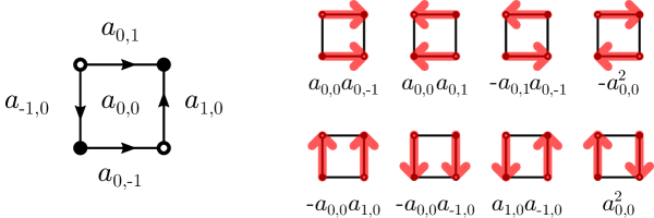
Figure 1: Left: the graph $G$ corresponding to one application of the dSKP equation, with a Kasteleyn orientation (showing the oriented edges $\vec{e}$ such that $\varphi_{\vec{e}}=1$). Right: its eight oriented dimers configurations, and their weights.

Another contribution of this paper is to show that the partition function $Z(G,a)$ can be expressed as a determinant. More precisely, the crosses and wrenches graph $G$ is bipartite so that its vertex set can be split into $V=W\sqcup B$; consider the weighted adjacency $K=(K_{w,b})$ of $G$, whose rows are indexed by white vertices of $W$, columns by black vertices of $B$, and whose non-zero entries are given by, for every edge $wb$ of $G$,

$$K_{w,b}=a_{f(w,b)}-a_{f(b,w)}.$$ (1.2)

Then, in Proposition 3.2, we prove that

$$Z(G,a,\varphi)=\pm\det(K).$$

It is to be noted that this exact matrix $K$ appears in the recent introduction of Coulomb gauges, or $t$-embeddings of dimer models. In [KLRR18] the authors start with a planar graph equipped with a standard dimer model, and (under some conditions) find an embedding of the dual graph: every face $f$ is sent to a point $a_{f}$. The Kasteleyn matrix of the initial dimer model is gauge equivalent to a matrix $K$ that is then exactly (1.2), therefore $\det(K)$ is the partition function of the initial dimer model. As a result, our approach may be seen as a way to expand the partition function of the initial dimer model in terms of these variables $a_{f}$, taken as formal variables, instead of the usual edge weights.

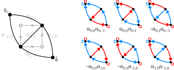
Figure 2: Left: the graph $G^{\bullet}$ in the running example; two vertices $b_{r},\tilde{b}$ have been added at the boundary. Right: its six complementary trees and forests configurations, and their weights. Forests are shown in red and may be rooted at $b_{r}$ or $\tilde{b}$, while trees are shown in blue and may only be rooted at $b_{r}$. Roots are represented by small loops.

Note that in the previous example, two configurations have weights that cancel each other. This is a generic fact which, for instance, occurs at all faces of degree 4 of $G$. Our next main contribution consists in introducing another model, whose partition function is equal to $Z(G,a,\varphi)$, but whose configurations are in one-to-one correspondence with the monomials in the $a$ variables. More precisely, in Section 4, for any quadrangulation $G$ of the sphere, we introduce a model of complementary trees and forests on the graph $G^{\bullet}$ formed by the black vertices of $G$ and diagonals joining them, with some boundary conditions. A configuration consists of two subsets $(\mathsf{T},\mathsf{F})$ of edges of $G^{\bullet}$ such that $\mathsf{T}$ is a spanning tree, and its complement $\mathsf{F}$ is a spanning forest, rooted at some specific vertices, see Section 4 for details, and Figure 2 for an example. We show the following, see also Theorem 4.2.

Theorem 1.3.

For any Kasteleyn orientation $\varphi$, the oriented dimer partition function is equal to

$$Z(G,a,\varphi)=\pm\sum_{(\mathsf{T},\mathsf{F})}\operatorname{sign}(\mathsf{T},\mathsf{F})\prod_{\vec{e}\in\mathsf{F}}a_{f_{\vec{e}}},$$

where the sum is over all complementary trees and forests configurations of $G^{\bullet}$. Moreover, there is a bijection between terms in the sum on the right-hand-side and monomials of $Z(G,a,\varphi)$ in the variables $a$.

The tools we develop to get the previous two results have several applications, in particular they allow us to study singularities of the dSKP recurrence. Although interesting in their own respect, the introduction of such singularities is motivated by their occurrence in geometric systems. The study of these systems and their singularities is the subject of the companion paper [AdTM22].

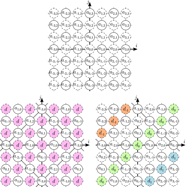
Figure 3: Initial data $(a_{i,j})$ for the dSKP recurrence, with height function $h(i,j)=[i+j]_{2}$. Variables in dashed circles lie at height $k=0$, while those in solid circles lie at height $k=1$. Top: generic. Bottom left: $3$-Dodgson; an elementary pattern is shown as a dashed square, and particular values at height $0$ are shown in purple. Bottom right: $(3,2)$-Devron; constant “columns” shown in orange, green, blue.

Consider the height function $h(i,j)=[i+j]_{2}$, so that the initial data $a=(a_{i,j})=(x(i,j,[i+j]_{2}))$ occupies heights $k=0$ and $k=1$ in $\mathcal{L}$. Suppose that all of the values at height $k=0$ are equal to a single value $d\in\hat{\mathbb{C}}$, and that values at height $k=1$ are $m$-doubly periodic, meaning that $a_{i,j}=a_{i+m,j+m}=a_{i+m,j-m}$; see Figure 3, bottom left. We call such initial data $m$-Dodgson initial conditions. In this case, the dSKP recurrence fails to define $x(i,j,k)$ for $k<0$, as trying to apply (1.1) leads to a singularity. However, getting the values at heights $k>1$ seems possible. As the dSKP recurrence is one of the octahedral consistent equations [ABS12], it is expected to have features common to integrable system, one of them being the Devron property [Gli15]: if some data is singular for the backwards dynamics, it should become singular after a finite number of applications of the forward dynamics. In our case, this means that at some height $k\geq 1$ (i.e. after $k-1$ iterations, understood as applications of the recurrence (1.1) to a whole level), all values of $x(i,j,k)$ will be equal. After this point the forward dynamics becomes impossible. We prove this Devron property, see also Section 5.5.

Theorem 1.4.

For $m$-Dodgson initial data, the values of $x$ are constant after $m-1$ iterations of the dSKP recurrence. In other words, for every $(i,j)\in\mathbb{Z}^{2}$ such that $(i,j,m)\in\mathcal{L}$, $x(i,j,m)$ is independent of $(i,j)$.

In fact, we prove a stronger invariance result for the corresponding partition function $Z(G,a,\varphi)$ itself (and not only the ratio), via the combinatorics of particular trees and forests configurations named permutation spanning forests, see Section 5.2, Theorems 5.4 and 5.6. As a consequence, we are able to explicitly compute this final value using the determinant and minors of the $m\times m$ matrix with entries $\frac{1}{a_{i,j}-d}$, which is reminiscent of Dodgson’s condensation [Dod67], hence the name of these initial data; see Corollary 5.7. Note that this matrix is much smaller than the previous matrix $K$, whose size is roughly $m^{2}\times m^{2}$. For instance, when $m=2$, a single iteration produces a constant layer; this can be seen in the running example, with $a_{0,0}$ playing the role of $d$. In this case, the explicit value of Corollary 5.7 uses the matrix

$$N=\begin{pmatrix}\frac{1}{a_{0,1}-a_{0,0}}&\frac{1}{a_{1,0}-a_{0,0}}\\ \frac{1}{a_{-1,0}-a_{0,0}}&\frac{1}{a_{0,-1}-a_{0,0}}\end{pmatrix}.$$ (1.3)

It states that

$$Z(G,a,\varphi)=\pm\prod_{i,j}(a_{i,j}-a_{0,0})\cdot\det N,$$

and that for any $(i,j)\in\mathbb{Z}^{2}$ with $[i+j]_{2}=0$,

$$x(i,j,2)=a_{0,0}+\sum_{i,j}\left(N^{-1}\right)_{i,j},$$ (1.4)

with the sum and product being over $(i,j)\in\{(0,1),(1,0),(0,-1),(-1,0)\}$.

Assuming more symmetries in the initial data, we prove an even simpler form for the final value.

Corollary 1.5.

For $m$-Dodgson initial data, suppose in addition that for some $p\not\in m\mathbb{Z}$, when $[i+j]_{2}=1$, $a_{i,j}=a_{i+p+1,j-p+1}$. Then after $m-1$ iterations of the dSKP recurrence, $x(i,j,m)$ is the shifted harmonic mean of the $m$ different values of the initial data:

$$x(i,j,m)=d+\left(\frac{1}{m}\sum_{i=0}^{m-1}\frac{1}{a_{i,1-i}-d}\right)^{-1}.$$

We then consider a generalization of Dodgson initial conditions. Suppose that the initial data is $m$-simply periodic, meaning that for all $(i,j)\in\mathbb{Z}^{2}$, $a_{i,j}=a_{i+m,j+m}$. We also assume that for some $p\geq 1$, for all $(i,j)\in\mathbb{Z}^{2}$ with $[i-j]_{2p}=0$, $a_{i,j}=a_{i+1,j+1}$. This amounts to having every $p$-th SW-NE diagonal at height $0$ constant, see Figure 3, bottom right; we denote these constant values by $a_{i,j}=:d_{(j-i)/(2p)}$. In this case, it is convenient to rotate the lattice by $45$ degrees, so the singularity becomes constant columns, which are easier to visualize; every $p$ column of height $0$ is constant. We call these $(m,p)$-Devron initial data. Again, we expect a Devron property to hold for this kind of singular data, which here means that at some height $k\geq 1$, values of $x(i,j,k)$ also have $p$-periodic constant columns.

Theorem 1.6.

For $(m,p)$-Devron initial data, let $k=(m-2)p+2$. Then after $k-1$ iterations of the dSKP recurrence, the values of $x$ also have $p$-periodic constant columns.

More precisely, for all $(i,j)\in\mathbb{Z}^{2}$ such that $[i-j-mp]_{2p}=0$,

$$x(i,j,k)=x(i+1,j+1,k).$$

When $p=1$, i.e., when all columns at height $0$ are constant, the proof of the strong invariance result of the $m$-Dodgson case also works, meaning that we have invariance of the partition function itself. For generic $p$ we cannot provide such a combinatorial proof – in fact the values of $Z(G,a,\varphi)$ are generically not invariant, while their ratio in Theorem 1.1 is – and we resort to more algebraic tools, in particular to Theorem 5.3.

Another case of study is when the initial data is periodic with respect to two non-colinear vectors $(s,t)$ and $(u,v)$ in $\mathbb{Z}^{2}$. We can also predict at which height singularities reoccur in that case, as consequences of Theorem 1.6; see Corollary 5.12.

As mentioned, such combinatorial solutions of discrete evolution equations are often related to limit shapes phenomena for the associated statistical mechanics models, which generalize the celebrated arctic circle phenomenon for tiling of the Aztec diamond [CEP⁺96, DFSG14, PS05, Mel18, Geo21]. In our case, it is unclear if one can hope for probabilistic interpretations of this sort for oriented dimers or complementary trees and forests, first because the solution is not a partition function but a ratio of partition functions, and second because configurations come with signs. However, by adapting the techniques developed in the previous references, we can compute the asymptotic behaviour of

$$\rho(i,j,k)=\dfrac{\partial x(i,j,k)}{\partial x(0,0,0)},$$

where $x(i,j,k)$ is understood as a function of initial conditions, among which $x(0,0,0)$. More precisely, we are able to study $\rho(i,j,k)$ when evaluated at some specific solutions of the dSKP recurrence, namely $x(i,j,k)=ia+jb+kc+d$ and $x(i,j,k)=a^{i}b^{j}c^{k}d$, where $a,b,c,d$ are real parameters, and $h(i,j)=[i+j]_{2}$. In these cases, we compute the asymptotics of $\rho(xk,yk,k)$ when $k\to\infty$, which depend on $x,y$. In some regimes of the $a,b,c,d$ parameters, this quantity behaves like $k^{-1}$ in some region of $x,y$ corresponding to an “arctic ellipse”, and decays exponentially outside of this region. For other choices of $a,b,c,d$, the behaviour is always exponential and sometimes divergent; all the exponential rates and prefactors are explicit. This is made precise in Proposition 6.1. In the absence of a probabilistic interpretation, we may still view this as a way to quantify the influence of initial conditions on solutions of the dSKP recurrence, in particular, an exponential divergence is indicative of a chaotic behaviour.

Finally, we give exact solutions for all other equations of the classification of integrable equations of octahedron type by Adler, Bobenko and Suris [ABS12]. In this reference the authors classify all equations on octahedra that satisfy some multi-dimensional consistency condition, up to admissible transformations, and come up with a finite list $\chi_{1},\dots,\chi_{5}$. Equation $\chi_{1}$ is the standard octahedron, or dKP, equation, whose solution was found by Speyer [Spe07] in terms of the dimer model; $\chi_{2}$ is the dSKP equation. In Theorem 7.2, we show how explicit solutions of the $\chi_{3},\chi_{4}$ and $\chi_{5}$ recurrences can be found from our $\chi_{2}$ solution as leading coefficient in certain expansions. Then, for $\chi_{4}$ and $\chi_{5}$, we also give direct combinatorial descriptions of these solutions, at least in the case of the height function $h(i,j)=[i+j]_{2}$.

Plan of the paper

In Section 2 we set up the definitions and recall Speyer’s solution of the dKP recurrence [Spe07]. In Section 3 we introduce the oriented dimer model, prove its determinantal structure, and state Theorem 3.4 (Theorem 1.1 of the introduction); we then prove it, extending some of Speyer’s tools and techniques. In Section 4 we introduce the complementary trees and forests model; we show how it relates generically to oriented dimers and Kasteleyn matrices, and we prove Theorem 4.2 (Theorem 1.3 of the introduction). Then in Section 5 we turn to the study of singularities of the dSKP recurrence, by studying oriented dimers, or trees and forests, on Aztec diamonds; we prove Theorem 1.4, Theorem 1.6, and Corollary 1.5. Section 6 is concerned with “limit shapes” phenomena, with a proper statement of the asymptotic behaviour of $\rho(i,j,k)$. Finally, in Section 7 we extend the combinatorial solution to all consistent equations of the octahedral family of [ABS12].

Acknowledgments

The first author would like to thank Boris Springborn and Sanjay Ramassamy for helpful discussions. He is supported by the Deutsche Forschungsgemeinschaft (DFG) Collaborative Research Center TRR 109 “Discretization in Geometry and Dynamics” as well as the by the MHI and Foundation of the ENS through the ENS-MHI Chair in Mathematics. The second and third authors are partially supported by the DIMERS project ANR-18-CE40-0033 funded by the French National Research Agency.

2 The dSKP recurrence & some tools of Speyer

In Section 2.1, we give a precise definition of the dSKP recurrence then, in Section 2.2, we introduce the crosses and wrenches construction of Speyer [Spe07] and, in order to put one of our main results (Theorem 3.4) into perspective, we state the result of [Spe07] on the dKP recurrence in Section 2.3.

2.1 Definition

The dSKP recurrence lives on vertices of the octahedral-tetrahedral lattice $\mathcal{L}$ defined as:

$$\mathcal{L}=\left\{p=(i,j,k)\in\mathbb{Z}^{3}:i+j+k\in 2\mathbb{Z}\right\}.$$

Projecting $\mathcal{L}$ vertically onto the plane yields the lattice $\mathbb{Z}^{2}$, whose bipartite coloring of the vertices corresponds to even and odd levels of $\mathcal{L}$.

Remark 2.1.

A somewhat more symmetric lattice that is in fact isomorphic to $\mathcal{L}$ is defined in [ABS12] as the root lattice:

$$Q(A_{3})=\{n=(n_{0},n_{1},n_{2},n_{3})\in\mathbb{Z}^{4}\mid n_{0}+n_{1}+n_{2}+n_{3}=0\}.$$

More precisely, an octahedral cell in $\mathcal{L}$ is given by six vertice $p\pm e_{i}$, where $p\in\mathbb{Z}^{3}\setminus\mathcal{L}$ and $(e_{i})_{i=1}^{3}$ is the canonical basis of $\mathbb{Z}^{3}$; in $Q(A_{3})$ they are $n+e_{i}+e_{j}$ where $n_{0}+n_{1}+n_{2}+n_{3}=-2$ and $\{i,j\}$ runs through the $6$ pair sets in $\{0,1,2,3\}$. An example of a graph isomorphism between $Q(A_{3})$ and $\mathcal{L}$ is $(n_{0},n_{1},n_{2},n_{3})\mapsto(n_{0}+n_{1},n_{0}+n_{2},n_{0}+n_{3})$ with inverse given by $(i,j,k)\mapsto\frac{1}{2}(i+j+k,i-j-k,-i+j-k,-i-j+k)$. These will be useful to translate some results of [ABS12] into our setting, see Section 7.

In this paper we use $\mathcal{L}$ even though its symmetries are less apparent, as we are interested in iterating an equation on octahedra towards the distinguished $e_{3}$ direction.

Up to now we have discussed the definition space of the dSKP recurrence, we now turn to the natural target space: the complex projective line ${\mathbb{C}\mathrm{P}}^{1}$. Consider the equivalence relation $\sim$ on $\mathbb{C}^{2}$ such that for $v,v^{\prime}\in\mathbb{C}^{2}$ we have $v\sim v^{\prime}$ if there is a $\lambda\in\mathbb{C}\setminus\{0\}$ such that $v=\lambda v^{\prime}$. Every point in the projective line is an equivalence class $[v]=\{v^{\prime}:v^{\prime}\sim v\}$ for some $v\in\mathbb{C}^{2}\setminus\{(0,0)\}$, thus

$${\mathbb{C}\mathrm{P}}^{1}=\{[v]:v\in\mathbb{C}^{2}\setminus\{(0,0)\}\}=\left(\mathbb{C}^{2}\setminus\{(0,0)\}\right)/\sim.$$

It is practical to consider an affine chart $\hat{\mathbb{C}}=\mathbb{C}\cup\{\infty\}$ of ${\mathbb{C}\mathrm{P}}^{1}$. Every point $z\in\mathbb{C}\subset\hat{\mathbb{C}}$ corresponds to $[z,1]$ in ${\mathbb{C}\mathrm{P}}^{1}$ and $\infty\in\hat{\mathbb{C}}$ corresponds to $[1,0]$. In the affine chart one can perform the usual arithmetic operations on ${\mathbb{C}\mathrm{P}}^{1}$. One can even apply the naive calculation rules $z+\infty=\infty,z/\infty=0$ etc., see [RG11, Section 17].

Definition 2.2.

A function $x:\mathcal{L}\rightarrow\hat{\mathbb{C}}$ satisfies the dSKP recurrence, if

$$\frac{(x_{-e_{3}}-x_{e_{2}})(x_{-e_{1}}-x_{e_{3}})(x_{-e_{2}}-x_{e_{1}})}{(x_{e_{2}}-x_{-e_{1}})(x_{e_{3}}-x_{-e_{2}})(x_{e_{1}}-x_{-e_{3}})}=-1.$$ (2.1)

holds evaluated at every point $p$ of $\mathbb{Z}^{3}\setminus\mathcal{L}$, where $x_{q}(p):=x(q+p)$ for every $q\in\{\pm e_{i}\}_{i=1}^{3}$. More generally, if $A\subset\mathcal{L}$ and $x:A\to\hat{\mathbb{C}}$, we say that $x$ satisfies the dSKP recurrence on $A$ when (2.1) hold whenever all the points are in $A$.

Remark 2.3.

1. By direct calculation, one sees that the dSKP recurrence features octahedral symmetry, i.e., if it holds then it is also satisfied for any permutation of the unit vectors $\{e_{1},e_{2},e_{3}\}$, and for any reflection $e_{i}\mapsto-e_{i}$.

2. A projective transformation $f:{\mathbb{C}\mathrm{P}}^{1}\rightarrow{\mathbb{C}\mathrm{P}}^{1}$ is a bijection such that there is a matrix $F\in\mathbb{C}^{2}\times\mathbb{C}^{2}$ with $f([v])=[Fv]$ for all $[v]\in{\mathbb{C}\mathrm{P}}^{1}$. Conversely, any matrix $F$ with $\det F\neq 0$ defines a projective transformation of ${\mathbb{C}\mathrm{P}}^{1}$. In an affine chart $\hat{\mathbb{C}}$, any projective transformation acts by $f(z)=\frac{az+b}{cz+d}$ for some $a,b,c,d\in\mathbb{C}$ with $ad-bc\neq 0$ and some special rules for $\infty$, in particular $f(\infty)=\frac{a}{c}$ and $f(-\frac{d}{c})=\infty$. It is a direct calculation to verify that the dSKP recurrence is invariant under projective transformations of $\hat{\mathbb{C}}$, and even by Möbius transformations, which are projective transformations possibly composed with complex conjugation $z\mapsto\bar{z}$. This is the first reason why $\hat{\mathbb{C}}$ is the natural target space for the dSKP recurrence.

3. The other reason is that if $x_{-e_{1}},x_{-e_{2}},x_{-e_{3}},x_{e_{1}},x_{e_{2}}$ are given such that

   $$x_{e_{1}}\neq x_{e_{2}},\ x_{e_{2}}\neq x_{-e_{1}},\ x_{-e_{1}}\neq x_{-e_{2}},\ x_{-e_{2}}\neq x_{e_{1}},$$

   then $x_{e_{3}}$ is well-defined by the dSKP recurrence, while this is not generally true in $\mathbb{C}$. In fact, if the condition above is satisfied, then there is a unique projective involution $f$ of ${\mathbb{C}\mathrm{P}}^{1}$ such that $f(x_{e_{1}})=x_{-e_{1}}$ and $f(x_{e_{2}})=x_{-e_{2}}$. A quick calculation shows that $f(x_{e_{3}})=x_{-e_{3}}$ if and only if dSKP is satisfied. However, $f(x_{e_{3}})$ may be $\infty$ which is fine in ${\mathbb{C}\mathrm{P}}^{1}$ but not in $\mathbb{C}$.

Example 2.4.

If $a,b,c,d\in\hat{\mathbb{C}}$, the function $x:\mathcal{L}\to\hat{\mathbb{C}}$ given by $x(i,j,k)=ia+jb+kc+d$ satisfies the dSKP recurrence. The same is true for the function $x(i,j,k)=a^{i}b^{j}c^{k}d$.

Following [Spe07, Section 2.1], we now define initial conditions for this recurrence. Let $h:\mathbb{Z}^{2}\to\mathbb{Z}$ be a function such that, forall $(i,j)\in\mathbb{Z}^{2}$, $(i,j,h(i,j))\in\mathcal{L}$, and consider the following subset of $\mathbb{Z}^{3}$ that will play the role of initial data locations for the dSKP recurrence:

$$\mathcal{I}_{h}=\{(i,j,h(i,j))\mid(i,j)\in\mathbb{Z}^{2}\}.$$ (2.2)

The idea is that, provided $h$ satisfies some extra conditions, fixing the values of $x$ at the points of $\mathcal{I}_{h}$ is enough to define $x$ on the upper set $\mathcal{U}_{h}$ of $h$, defined as

$$\mathcal{U}_{h}=\{(i,j,k)\in\mathcal{L}\mid k>h(i,j)\}.$$ (2.3)

When there is no ambiguity, we will simply denote these by $\mathcal{I},\mathcal{U}$.

To define these extra conditions on $h$, we introduce the closed (resp. open) square cone of a vertex $(i,j,k)\in\mathcal{L}$ (roughly speaking a semi-infinite square-pyramid with its tip at $(i,j,k)$, see Figure 4):

$$\begin{split}\mathcal{C}_{(i,j,k)}&=\{(i^{\prime},j^{\prime},k^{\prime})\in\mathcal{L}\mid k^{\prime}\leq k-|i-i^{\prime}|-|j-j^{\prime}|\}\\ \mathring{\mathcal{C}}_{(i,j,k)}&=\{(i^{\prime},j^{\prime},k^{\prime})\in\mathcal{L}\mid k^{\prime}<k-|i-i^{\prime}|-|j-j^{\prime}|\}.\end{split}$$ (2.4)

We say that $h$ is a height function if the following holds:

1. If $(i,j)$ and $(i^{\prime},j^{\prime})$ are neighbors in $\mathbb{Z}^{2}$, then $|h(i,j)-h(i^{\prime},j^{\prime})|=1$,

2. $\lim_{|i|+|j|\to\infty}h(i,j)+|i|+|j|=\infty$.

Consider a height function $h$, and an initial condition $a$, that is a function $a:\mathbb{Z}^{2}\rightarrow\mathbb{C}$ such that on $\mathcal{I}$,

$$x(i,j,h(i,j))=a_{i,j}.$$

Our goal is to analyze the solution $x$ to the dSKP recurrence on the set $\mathcal{I}\cup\mathcal{U}$ when the initial condition on $\mathcal{I}$ is given by $a$. Note that Condition 2. is equivalent to the fact that for any $p\in\mathcal{L}$, $\mathcal{C}_{p}\cap\mathcal{U}$ is finite [Spe07].

2.2 Crosses and wrenches construction

Let us now turn to the crosses and wrenches construction of Speyer [Spe07, Section 3]. All graphs considered are simple, connected, planar and embedded, implying that they also have faces; in order to alleviate the text, these assumptions will not be repeated.

We first need the definition of a graph with open faces. Consider a finite graph $G=(V,E)$. Denote by $F^{i}$ the set of internal faces. Partition the external boundary into sets of adjacent edges; this partitions the outer face into a finite number of faces referred to as open faces and denoted by $F^{o}$. Set $F=F^{i}\cup F^{o}$.

Given a height function $h$, Speyer defines an infinite graph $\mathcal{G}$, referred to as the (infinite) crosses and wrenches graph, in the following way. Faces of $\mathcal{G}$ are indexed by points of $\mathcal{I}$, and are in bijection with $\mathbb{Z}^{2}$: the face corresponding to $(i,j,h(i,j))$ is centered at the vertex $(i,j)$ of $\mathbb{Z}^{2}$. Every unit square of $\mathbb{Z}^{2}$ is bounded by four vertices corresponding to four faces of $\mathcal{G}$; the way the four faces meet depends on the values of $h$ at the vertices. Since $h$ is a height function, we are in one of the following cases: either both diagonally opposite heights are equal (and differ by 1), in which case we put a “cross” (a vertex of degree $4$) at the intersection of the four faces; or two diagonally-opposite faces have the same height $h_{0}$, and the other two have heights $h_{0}-1$ and $h_{0}+1$ respectively, in which case we put a “wrench” (an edge with two endpoints of degree $3$) where those four faces meet, with the “handle” separating the faces of height $h_{0}$, see Figure 4 (center) for an example, and [Spe07] for more details. Note that the graph $\mathcal{G}$ is bipartite with faces of degree 4, 6 or 8.

Then, to every point $p$ of $\mathcal{U}$, one assigns a finite subgraph with open faces of $\mathcal{G}$, denoted by $G_{p}=(V_{p},E_{p})$ and referred to as the crosses and wrenches graph corresponding to $p$, constructed as follows. The internal faces $F_{p}^{i}$ are indexed by elements of $\mathcal{I}\cap\mathring{\mathcal{C}}_{p}$, and the edges $E_{p}$ and vertices $V_{p}$ are those of $\mathcal{G}$ that belong to at least one of these faces. The open faces $F_{p}^{o}$ are indexed by the elements of $\mathcal{I}$ that share some (but not all) edge(s) with $E_{p}$; note that there are no edges separating open faces. We have $F_{p}=F_{p}^{i}\cup F_{p}^{o}$. The vertices of the external face that separate open faces are called boundary vertices and their set is denoted by $\partial V_{p}\subset V_{p}$; see again Figure 4. Whenever no confusion occurs, we will remove the subscript $p$ from the notation. Each face $f$ of $F$ corresponds to some $(i,j,h(i,j))$ in $\mathcal{I}$ and to some $(i,j)$ in $\mathbb{Z}^{2}$, and we assign it a weight

$$a_{f}=a_{i,j}=x(i,j,h(i,j)),$$

corresponding to the initial condition $a$ for the dSKP recurrence. The degree $d(f)$ of the face $f$ is defined as the number of edges of $G_{p}$ adjacent to $f$.

Figure 4: Left: for $(i,j,k)=(0,0,4)$, the function $(i^{\prime},j^{\prime})\mapsto k-|i-i^{\prime}|-|j-j^{\prime}|$ that defines the closed square cone $\mathcal{C}_{(0,0,4)}$. Center: a height function $h:\mathbb{Z}^{2}\to\mathbb{Z}$, with the corresponding crosses and wrenches graph $\mathcal{G}$; the places where $(i^{\prime},j^{\prime},h(i^{\prime},j^{\prime}))\in\mathring{\mathcal{C}}_{(0,0,4)}$, i.e., where the height is strictly smaller than on the left, are colored in gray. Right: the graph $G_{(0,0,4)}$, equipped with the corresponding variables $a_{i,j}=x(i,j,h(i,j))$. The vertices of $\partial V_{(0,0,4)}$ are shown in blue and joined by a dashed “boundary”.

2.3 dKP recurrence

In [Spe07], Speyer solved the case of the dKP or octahedron recurrence , and a correspondence with the dimer model was established. In order to make the context of the present paper more clear, and to put our forthecoming Theorem 3.4 into perspective, we rephrase these results in our notation.

Definition 2.5.

A function $x:\mathcal{L}\rightarrow\hat{\mathbb{C}}$ satisfies the dKP or octahedron recurrence if

$$x_{e_{3}}x_{-e_{3}}=x_{e_{1}}x_{-e_{1}}+x_{e_{2}}x_{-e_{2}},$$

holds evaluated at any $p$ of $\mathbb{Z}^{3}\setminus\mathcal{L}$.

The main result of Speyer [Spe07] relies on the following definitions. Let $G$ be a finite graph. Then, a dimer configuration $\mathsf{M}$ of $G$, or perfect matching, is a subset of edges such that every vertex of $G$ is incident to exactly one edge of $\mathsf{M}$; we denote by $\mathscr{M}$ the set of dimer configurations of $G$. When $G$ is a graph with open faces $F=F^{i}\cup F^{o}$, equipped with face weights $(a_{f})_{f\in F}$, define the weight of $\mathsf{M}$ as

$$w(\mathsf{M})=\prod_{e\in\mathsf{M}}\frac{1}{a_{f(e)}a_{f^{\prime}(e)}},$$

where $f(e),f^{\prime}(e)$ denote the two faces adjacent to $e$. The corresponding partition function, denoted $Z_{\text{dim}}(G,a)$, is

$$Z_{\mathrm{dim}}(G,a)=\sum_{\mathsf{M}\in\mathscr{M}}w(\mathsf{M}).$$

Theorem 2.6 ([Spe07]).

Let $x:\mathcal{L}\rightarrow\hat{\mathbb{C}}$ be a function that satisfies the dKP recurrence. Let $h$ be a height function, and $\mathcal{I},\mathcal{U}$ be defined as in Equations (2.2), (2.3). Let $a=(a_{i,j})=(x(i,j,h(i,j)))$ be the initial data indexed by points of $\mathcal{I}$. Then for every point $p$ of $\mathcal{U}$,

$$x(p)=C_{\mathrm{dim}}(G_{p},a)\cdot\ Z_{\mathrm{dim}}(G_{p},a),$$

where

$$C_{\mathrm{dim}}(G_{p},a)=\prod_{f=(i,j)\in F_{p}^{i}}a_{i,j}^{\frac{d(f)}{2}-1}\prod_{f=(i,j)\in F_{p}^{o}}a_{i,j}^{\lceil\frac{d(f)}{2}\rceil},$$

and $G_{p}$ is the crosses and wrenches graph corresponding to $p$.

3 dSKP: combinatorial solution I - oriented dimers

In Section 3.1, we state Theorem 3.4, our main result on the dSKP recurrence. In Section 3.2, we introduce the ratio function of oriented dimers in the setting of infinite completions, a tool that allows to smoothly handle boundary issues. Then, in Section 3.3, we prove invariance of the ratio function under two types of moves on the underlying graph, namely contraction/expansion of a degree 2 vertex and urban renewal. Using all this we proceed with the proof of Theorem 3.4 in Section 3.4, following an argument of [Spe07].

3.1 Definitions and main dSKP theorem

Consider a finite, bipartite graph $G$ with open faces $F=F^{i}\cup F^{o}$, equipped with faces weights $(a_{f})_{f\in F}$. The set of vertices $V$ is naturally split into black and white, $V=B\sqcup W$, and from now on we assume that $|W|=|B|$. Denote by $\vec{E}$ the set of directed edges of $G$, i.e., given an edge $wb$ of $E$ there corresponds two directed edges $(w,b)$, $(b,w)$ of $\vec{E}$; when vertices are not specified a directed edge is also denoted as $\vec{e}$.

A Kasteleyn orientation [Kas61] is a skew-symmetric function $\varphi$ from $\vec{E}$ to $\{-1,1\}$ such that, for every internal face $f$ of $F^{i}$ of degree $2k$, we have

$$\prod_{wb\in\partial f}\varphi_{(w,b)}=(-1)^{k+1}.$$

This corresponds to an orientation of edges of the graph: an edge $e=wb$ is oriented from $w$ to $b$ when $\varphi_{(w,b)}=1$, and from $b$ to $w$ when $\varphi_{(w,b)}=-1$. By Kasteleyn [Kas67], such an orientation exists when $G$ is planar.

An oriented dimer configuration of $G$ is a subset of oriented edges $\vec{\mathsf{M}}$ such that its undirected version $\mathsf{M}$ is a dimer configuration. Denote by $\vec{\mathscr{M}}$ the set of oriented dimer configurations of $G$. Note that given a dimer configuration $\mathsf{M}$ there corresponds $2^{|\mathsf{M}|}$ oriented dimer configurations, where $|\mathsf{M}|$ denotes the number of edges of $\mathsf{M}$.

Given a Kasteleyn orientation $\varphi$, and an oriented edge $\vec{e}$, denote by $f(\vec{e})$ the (inner or open) face to the right of $\vec{e}$. The weight of an oriented dimer configurations $\vec{\mathsf{M}}$ is

$$w(\vec{\mathsf{M}})=\prod_{\vec{e}\in\vec{\mathsf{M}}}\varphi_{\vec{e}}\ a_{f(\vec{e})},$$

and the corresponding partition function is

$$Z(G,a,\varphi)=\sum_{\vec{\mathsf{M}}\in\vec{\mathscr{M}}}w(\vec{\mathsf{M}}).$$

Remark 3.1.

By grouping the two possible orientations of an edge, the partition function can be rewritten as

$$Z(G,a,\varphi)=\sum_{\mathsf{M}\in\mathscr{M}(G)}\prod_{wb\in\mathsf{M}}\varphi_{(w,b)}(a_{f(w,b)}-a_{f(b,w)}).$$ (3.1)

It is thus the partition function of usual dimers, with edge weights $(\varphi_{(w,b)}(a_{f(w,b)}-a_{f(b,w)}))_{wb\in E}$.

As we will now see, this quantity depends on $\varphi$ only up to a global sign.

Let $K=(K_{w,b})$ be the weighted adjacency matrix of $G$, whose rows are indexed by white vertices of $W$, columns by black vertices of $B$, and whose non-zero entries are given by, for every edge $wb$ of $G$,

$$K_{w,b}=a_{f(w,b)}-a_{f(b,w)}.$$

Then we prove the following.

Proposition 3.2.

For every finite, bipartite graph $G$ with open faces, weights $a=(a_{f})_{f\in F}$ on the faces, and Kasteleyn orientation $\varphi$, there exists $\epsilon(\varphi)\in\{-1,+1\}$ depending on $\varphi$ only, such that

$$Z(G,a,\varphi)=\epsilon(\varphi)\det(K).$$

Proof.

Using the alternative expression (3.1) and the Kasteleyn theory [Kas61], see also [TF61, Per69], we know that, up to a sign depending on $\varphi$ only, the partition function $Z(G,a,\varphi)$ is equal to the determinant of the Kasteleyn matrix corresponding to $\varphi$, which is the weighted adjacency matrix whose non-zero coefficients are given by, for every edge $wb$,

$$\varphi_{(w,b)}\cdot\varphi_{(w,b)}(a_{f(w,b)}-a_{f(b,w)})=a_{f(w,b)}-a_{f(b,w)},$$

i.e., it is equal to the determinant of the matrix $K$. ∎

Definition 3.3.

Consider a finite, bipartite graph $G$ with open faces, together with face weights $a=\left(a_{f}\right)_{f\in F}$ in $\hat{\mathbb{C}}$, and a Kasteleyn orientation $\varphi$. When it is well-defined in $\hat{\mathbb{C}}$, we denote the ratio function of oriented dimers as

$$Y(G,a)=C(G,a)\ \frac{Z(G,a^{-1},\varphi)}{Z(G,a,\varphi)},$$ (3.2)

where $a^{-1}=\bigl{(}a^{-1}_{f}\bigr{)}_{f\in F}$ and

$$C(G,a)=i^{|V|}\prod_{f\in F^{i}}a_{f}^{\frac{d(f)}{2}-1}\prod_{f\in F^{o}}a_{f}^{\lceil\frac{d(f)}{2}\rceil}.$$

By Proposition 3.2, the ratio in Equation (3.2) does not depend on $\varphi$, hence the same goes for $Y(G,a)$. The normalization $C(G,a)$, as we will see in the next paragraph, is such that $Y(G,a)$ is invariant under several local modifications of the weighted graph $(G,a)$.

We can now precisely state the main result of this section, which is the pendent of Speyer’s Theorem 2.6 in the case of the dSKP recurrence. Note that it involves a ratio of partition functions rather than only a partition function as in [Spe07].

Theorem 3.4.

Let $x:\mathcal{L}\rightarrow\hat{\mathbb{C}}$ be a function that satisfies the dSKP recurrence. Let $h$ be a height function, and $\mathcal{I},\mathcal{U}$ be defined as in Equations (2.2), (2.3). Let $(a_{i,j})=(x(i,j,h(i,j)))$ be the initial data indexed by points of $\mathcal{I}$. Then for every point $p$ of $\mathcal{U}$,

$$x(p)=Y(G_{p},a),$$

where $G_{p}$ is the crosses and wrenches graph corresponding to $p$.

Before proving Theorem 3.4, let us illustrate this theorem with an example.

Example 3.5 (Aztec diamond).

Consider the height function $h:\mathbb{Z}^{2}\to\{0,1\}$, given by $h(i,j)=[i+j]_{2}$. Let $x:\mathcal{L}\to\hat{\mathbb{C}}$ be a function that satisfies the dSKP recurrence. The initial data are again $(a_{i,j})=(x(i,j,h(i,j)))$. For $p=(i,j,k+1)\in\mathcal{L}$, let us explicitly describe $x(p)$ in terms of the initial data.

In the cross and wrenches construction, this height function $h$ only produces crosses. The crosses and wrenches graph $G_{p}$ is commonly known as the Aztec diamond of size $k$, where the size is the number of squares per “side” of the Aztec diamond, and the central face is at $(i,j)$; in this case, the graph $G_{p}$ is commonly denoted by $A_{k}$; see Figure 5. Using Theorem 3.4 and computing the prefactor in Equation (3.2), we get that for $k\geq 1$, the value of $x(p)$ is

$$x(p)=Y(A_{k},a)=\biggl{(}\,\prod_{f\in F_{p}}a_{f}\biggr{)}\frac{Z(A_{k},a^{-1},\varphi)}{Z(A_{k},a,\varphi)},$$ (3.3)

where the product is over all faces of $A_{k}$, internal or open, and the values of $a$ are displayed in Figure 5.

Figure 5: Left: the cross and wrenches graphs in Example 3.5, for $k=3,p=(0,0,4)$. The height function $h$ is shown in black, and the function defining $\mathcal{C}_{p}$ is shown in red, giving the finite graph with open faces $G_{p}$ (gray); in this case, it is an Aztec diamond of size $k=3$ centered at face $(i,j)=(0,0)$, denoted by $A_{k}$. Right: the same graph with open faces with its face weights $a$; every gray dot represents a face (inner or open) and is equipped with a weight.

Remark 3.6.

Note that oriented dimer configurations and monomials of $Z(A_{k},a,\varphi)$ in the $a$ variables in the denominator of Equation (3.3) are not in one-to-one correspondence. The same of course also holds true for the numerator of (3.3). For instance, for $k=1$ there are $8$ oriented dimer configurations but $6$ monomials; for $k=2$ there are $512$ configurations but $220$ monomials; for $k=3$ there are $262144$ configurations but $49224$ monomials. Unfortunately the sequence of number of monomials is not in OEIS.

What happens is that several oriented dimer configurations cancel each other. An example is when a square face is surrounded by two clockwise dimers. Changing these dimers by the other two edges, oriented clockwise, has the effect of negating the weight. As a result, the variables $a$ can only appear with exponent $1$ in the monomials.

Finding a model that gives such a one-to-one correspondence is one of the goals of Section 4, and the final statement for the Aztec diamond is given in Corollary 5.1.

The proof of Theorem 3.4 is the subject of the next three sections. The method follows that of Speyer [Spe07]. The first part, Section 3.2, relates dimers on $G_{p}$ to dimers on an infinite graph, with some asymptotic conditions; this trick is useful to get rid of issues at the boundary. The second part, Section 3.3, consists in proving that $Y(G,a)$ is invariant under natural modifications of the underlying graph and weight function. The third part, Section 3.3, relies on the first two and is an induction argument on the height functions. Note that the main contributions of Theorem 3.4 are the identification of the function $Y(G_{p},a)$ satisfying the invariance relations and handling ratios of partition functions in the proof.

3.2 Infinite completions

We follow [Spe07, Section 4.1] for the following definition. Consider a height function $h$, a point $p=(i,j,k)\in\mathcal{U}_{h}$, and introduce the function

$$h_{p}(i^{\prime},j^{\prime})=\min\left(h(i^{\prime},j^{\prime}),k-|i-i^{\prime}|-|j-j^{\prime}|\right).$$ (3.4)

Note that the minimum is between $h$ and the function defining $\mathcal{C}_{p}$. Then $h_{p}$ is not a height function, as it does not satisfy Condition 2. but, since it still satisfies Condition 1., we may produce an infinite graph $\mathcal{G}_{p}$ from $h_{p}$ using the method of crosses and wrenches. Then $G_{p}$ is also a subgraph of $\mathcal{G}_{p}$, consisting of hexagons at face distance 1 from $G_{p}$, see Figure 6.

Figure 6: The function $h_{p}$ and the corresponding infinite graph $\mathcal{G}_{p}$, using the same example as Figure 4. The subgraph $G_{p}$ is colored in gray. An admissible dimer configuration is shown in red.

A perfect matching $\mathsf{M}$ on $\mathcal{G}_{p}$ is said to be acceptable if there exists a finite subgraph outside of which $\mathsf{M}$ contains only the middle edge of every wrench. We denote by $\mathscr{M}_{\infty}\bigl{(}\mathcal{G}_{p}\bigr{)}$ the set of acceptable perfect matchings of $\mathcal{G}_{p}$. By [Spe07, Proposition 6], acceptable perfect matchings on $\mathcal{G}_{p}$ are in bijection with perfect matchings of $G_{p}$, and can in fact always be obtained by extending a perfect matching of $G_{p}$ to $\mathcal{G}_{p}$ using all wrenches of $\mathcal{G}_{p}\setminus G_{p}$; see also Figure 6.

The introduction of ratios of partition functions on the infinite graph $\mathcal{G}_{p}$ requires a bit more care than in [Spe07], as we would like to develop and factor infinite products of face weights in two partition functions, and then simplify them; these last steps were not required in [Spe07]. We proceed in the following way: fix an acceptable perfect matching $\mathsf{M}_{0}\in\mathscr{M}_{\infty}\bigl{(}\mathcal{G}_{p}\bigr{)}$, then for any $\mathsf{M}\in\mathscr{M}_{\infty}\bigl{(}\mathcal{G}_{p}\bigr{)}$, $\mathsf{M}_{0}$ and $\mathsf{M}$ differ only at a finite number of edges, hence the following ratio of weights is well-defined:

$$\frac{w_{\infty}(\mathsf{M})}{w_{\infty}(\mathsf{M}_{0})}=\frac{\prod_{wb\in\mathsf{M}\setminus\mathsf{M}_{0}}\varphi_{(w,b)}\left(a_{f(w,b)}-a_{f(b,w)}\right)}{\prod_{wb\in\mathsf{M}_{0}\setminus\mathsf{M}}\varphi_{(w,b)}\left(a_{f(w,b)}-a_{f(b,w)}\right)}.$$ (3.5)

We define the partition function relative to $\mathsf{M}_{0}$ as

$$Z_{\infty}\left(\mathcal{G}_{p},a,\varphi,\mathsf{M}_{0}\right)=\sum_{\mathsf{M}\in\mathscr{M}_{\infty}\left(\mathcal{G}_{p}\right)}\frac{w_{\infty}(\mathsf{M})}{w_{\infty}(\mathsf{M}_{0})}.$$ (3.6)

Let $\mathcal{F}_{p}$ be the set of faces of $\mathcal{G}_{p}$. For any $f\in\mathcal{F}_{p}$, let $d_{\mathsf{M}_{0}}(f)$ be the number of dimers in $\mathsf{M}_{0}$ adjacent to $f$. Note that all but a finite number of faces $f\in\mathcal{F}_{p}$ have degree $6$ and are such that $d_{\mathsf{M}_{0}}(f)=2$. This implies that the prefactor in the following expression is well-defined:

$$Y_{\infty}\left(\mathcal{G}_{p},a\right)=\left(\prod_{f\in\mathcal{F}_{p}}a_{f}^{\frac{d(f)}{2}-1-d_{\mathsf{M}_{0}}(f)}\right)\frac{Z_{\infty}\left(\mathcal{G}_{p},a^{-1},\varphi,\mathsf{M}_{0}\right)}{Z_{\infty}\left(\mathcal{G}_{p},a,\varphi,\mathsf{M}_{0}\right)}.$$ (3.7)

As suggested by the notation, $Y_{\infty}\left(\mathcal{G}_{p},a\right)$ does not depend on $\mathsf{M}_{0}$ nor on $\varphi$; this will be a consequence of the forthcoming Proposition 3.7.

The main point of this construction is that, since $\mathcal{G}_{p}$ has no outer face, the quantity $Y_{\infty}$ treats internal and outer faces in the same way. Together with the next proposition, which states that using $\mathcal{G}_{p}$ we recover the usual ratio of partition functions on $G_{p}$, this allows us to avoid tedious case handling at the boundary.

Proposition 3.7.

Let $h$ be a height function, let $p\in\mathcal{U}_{h}$, let $h_{p}$ be defined by (3.4), and let $\mathcal{G}_{p}$ be the crosses and wrenches graph corresponding to $h_{p}$. Then

$$Y_{\infty}\left(\mathcal{G}_{p},a\right)=Y(G_{p},a).$$

Proof.

Recall that $E_{p}$ are the edges of the finite subgraph $G_{p}$. Again by [Spe07, Proposition 6],

$$Z_{\infty}\left(\mathcal{G}_{p},a,\varphi,\mathsf{M}_{0}\right)=\frac{Z(G_{p},a,\varphi)}{\prod_{wb\in\mathsf{M}_{0}\cap E_{p}}\varphi_{(w,b)}\left(a_{f(w,b)}-a_{f(b,w)}\right)}.$$

Doing the same for face weights $a^{-1}$ and taking the ratio, we get

$$\begin{split}\frac{Z_{\infty}\left(\mathcal{G}_{p},a^{-1},\varphi,\mathsf{M}_{0}\right)}{Z_{\infty}\left(\mathcal{G}_{p},a,\varphi,\mathsf{M}_{0}\right)}=&\biggl{(}\,\prod_{wb\in\mathsf{M}_{0}\cap E_{p}}\frac{a_{f(w,b)}-a_{f(b,w)}}{a^{-1}_{f(w,b)}-a^{-1}_{f(b,w)}}\biggr{)}\frac{Z(G_{p},a,\varphi)}{Z(G_{p},a^{-1},\varphi)},\\ =&(-1)^{|\mathsf{M}_{0}\cap E_{p}|}\biggl{(}\,\prod_{wb\in\mathsf{M}_{0}\cap E_{p}}a_{f(w,b)}a_{f(b,w)}\biggr{)}\frac{Z(G_{p},a,\varphi)}{Z(G_{p},a^{-1},\varphi)}.\end{split}$$ (3.8)

Therefore,

$$Y_{\infty}\left(\mathcal{G}_{p},a\right)=(-1)^{|\mathsf{M}_{0}\cap E_{p}|}\biggl{(}\,\prod_{f\in\mathcal{F}_{p}}a_{f}^{\frac{d(f)}{2}-1-d_{\mathsf{M}_{0}}(f)}\biggr{)}\biggl{(}\,\prod_{wb\in\mathsf{M}_{0}\cap E_{p}}a_{f(w,b)}a_{f(b,w)}\biggr{)}\frac{Z(G_{p},a,\varphi)}{Z(G_{p},a^{-1},\varphi)}.$$

We claim that

$$(-1)^{|\mathsf{M}_{0}\cap E_{p}|}\biggl{(}\,\prod_{f\in\mathcal{F}_{p}}a_{f}^{\frac{d(f)}{2}-1-d_{\mathsf{M}_{0}}(f)}\biggr{)}\biggl{(}\,\prod_{wb\in\mathsf{M}_{0}\cap E_{p}}a_{f(w,b)}a_{f(b,w)}\biggr{)}=i^{|V_{p}|}\prod_{f\in F_{p}^{i}}a_{f}^{\frac{d(f)}{2}-1}\prod_{f\in F_{p}^{o}}a_{f}^{\lceil\frac{d(f)}{2}\rceil},$$ (3.9)

which implies that $Y_{\infty}\left(\mathcal{G}_{p},a\right)=Y(G_{p},a)$. First, $\mathsf{M}_{0}$ reduces to a perfect matching of $G_{p}$, so $|M_{0}\cap E_{p}|=\frac{|V_{p}|}{2}$, proving that the complex prefactors are the same. Then, let $f\in\mathcal{F}_{p}$. If $f\notin F_{p}$, as argued previously, $a_{f}$ has exponent $0$ in the left-hand side of (3.9), in accordance with the right-hand side. If $f\in F_{p}^{i}$, then the second product on the left-hand side of (3.9) produces a factor $a_{f}^{d_{\mathsf{M}_{0}}(f)}$, simplifying with the first product to give $a_{f}^{\frac{d(f)}{2}-1}$ as on the right-hand side. Finally, if $f\in F_{p}^{o}$, then by the same argument, the left-hand side gives an exponent $\frac{d(f)}{2}-1-d_{\mathsf{M}_{0}\setminus E_{p}}(f)$, which exactly corresponds to the normalization obtained for acceptable dimers in [Spe07, Section 4.1] (we recall that in Speyer’s case, the weight of an edge $wb$ is $\frac{1}{a_{f(w,b)}a_{f(b,w)}}$, so the dimers in $\mathsf{M}$ outside of $G_{p}$ contribute with a factor $a_{f}^{-d_{\mathsf{M}\setminus E_{p}}(f)}$). By Speyer’s computation, this is equal to the normalization in $C_{\mathrm{dim}}(G_{p},a)$ for this face, which is also $\lceil\frac{d(f)}{2}\rceil$. ∎

3.3 Invariance of ratio function of oriented dimers

In this section, $G$ is a finite bipartite graph with open faces $F=F^{i}\cup F^{o}$, equipped with face weights $a=\left(a_{f}\right)_{f\in F}$. We will often identify the names of faces with the weights attached to it.

3.3.1 Contraction/Expansion of a vertex of degree 2

In the graph $G$, consider a vertex $v$ adjacent to at least two distinct inner faces with respective weights $a_{1},a_{2}$. A new graph $G^{\prime}$ can be obtained by replacing $v$ with two vertices $v_{1},v_{2}$ joined by a vertex $u$ of degree $2$, such that the two new edges separate $a_{1}$ from $a_{2}$; see Figure 7.

This produces $G^{\prime}$ which is also bipartite, and naturally equipped with face weights still denoted by $a$. The graphs $G$ and $G^{\prime}$ are said to be related by the contraction/expansion of a vertex of degree $2$.

Figure 7: Local operation of contracting/expanding a vertex of degree $2$, with an example Kasteleyn orientation on the expanded side.

Proposition 3.8.

Let $G$, $G^{\prime}$ be two graphs as above related by the contraction/expansion of a vertex of degree $2$. Then

$$Y(G,a)=Y(G^{\prime},a).$$

Proof.

Suppose that the vertex $v$ is black, the case where $v$ is white being similar. Let $\varphi$ be a Kasteleyn orientation on $G$. We can get a Kasteleyn orientation of $G^{\prime}$, also denoted $\varphi$, by setting $\varphi_{(u,v_{1})}=1$, $\varphi_{(u,v_{2})}=-1$, see Figure 7. As $Y(G^{\prime},a)$ does not depend on the Kasteleyn orientation, we can use $\varphi$ in the proof.

We claim that $Z(G^{\prime},a,\varphi)=(a_{2}-a_{1})Z(G,a,\varphi)$. Indeed, using Expression (3.1) for the partition function, in a perfect matching of $G^{\prime}$, $u$ has to be matched either to $v_{1}$ or to $v_{2}$. In the first case, this gives a contribution $(a_{2}-a_{1})$ that factors in the corresponding sub-sum of $Z(G^{\prime},a,\varphi)$, and in the second case, it gives a contribution $-1(a_{1}-a_{2})=a_{2}-a_{1}$ to the second sub-sum. As the sum of these two sub-sums is $Z(G,a,\varphi)$, we get the claim.

Therefore, $Z(G^{\prime},a^{-1},\varphi)=\left(a_{2}^{-1}-a_{1}^{-1}\right)Z(G,a^{-1},\varphi)$, from which we get

$$-a_{1}a_{2}\frac{Z(G^{\prime},a^{-1},\varphi)}{Z(G^{\prime},a,\varphi)}=\frac{Z(G,a^{-1},\varphi)}{Z(G,a,\varphi)}.$$

Accounting for the discrepancy of degree of faces $a_{1},a_{2}$ between $G$ and $G^{\prime}$, it is straightforward to check that $Y(G,a)=Y(G^{\prime},a)$. Note that this is where we use the hypothesis that faces $a_{1},a_{2}$ are inner faces. ∎

3.3.2 Urban renewal

We state the central invariance result, which is the application of an urban renewal, also known as a square move, a spider move [Pro03, Ciu03]. Suppose that $G$ contains a face of degree four, with vertices $\{v_{1},v_{2},v_{3},v_{4}\}$ in counterclockwise cyclic order, surrounded by four distinct (inner or open) faces; the vertices $v_{i}$ may belong to $\partial V$ or not. Then we replace this square with a smaller one surrounded by four edges, as in Figure 8, and obtain a graph denoted by $G^{\prime}$.

Suppose that $G$ has face weights $a$; denote by $a_{0,0}$ the weight of the center face, and by $a_{-1,0},a_{0,-1},a_{1,0},a_{0,1}$ the weights at the four boundary faces. Then, we set $G^{\prime}$ to have a weight function $a^{\prime}$ equal to $a$ everywhere except at the center face where it is equal to $a_{0,0}^{\prime}$.

Definition 3.9.

Under the above assumptions, the weight functions $a$ and $a^{\prime}$ are said to satisfy the dSKP relation if:

$$\frac{(a_{0,0}-a_{0,1})(a_{-1,0}-a_{0,0}^{\prime})(a_{0,-1}-a_{1,0})}{(a_{0,1}-a_{-1,0})(a_{0,0}^{\prime}-a_{0,-1})(a_{1,0}-a_{0,0})}=-1.$$ (3.10)

Remark 3.10.

Note that by setting $x_{i,j,0}=a_{i,j}$ whenever $i$ or $j$ is equal to $\pm 1$, and $x_{-e_{3}}=x_{0,0,-1}=a_{0,0}$, $x_{e_{3}}=x_{0,0,1}=a_{0,0}^{\prime}$, we recover the dSKP recurrence of Definition 2.2 evaluated at the point $p=(0,0,0)$.

Figure 8: The “urban renewal” transformation; the Greek letters represent the Kasteleyn orientation, and non-indexed edges on the right-hand side are given orientation $1$, i.e., from white to black.

Proposition 3.11.

Let $G,G^{\prime}$ be two graphs as above related by an urban renewal, and suppose that the respective weight functions $a$ and $a^{\prime}$ (as in Figure 8) satisfy the dSKP relation (3.10). Then

$$Y(G,a)=Y(G^{\prime},a^{\prime}).$$

Proof.

Fix a Kasteleyn orientation $\varphi$ on $G$. We get a Kasteleyn orientation on $G^{\prime}$ as in Figure 8, by multiplying $\varphi$ by $-1$ on the square and setting it to $1$ on the four newly created edges; we denote it by $\varphi^{\prime}$.

Consider a perfect matching on $G$ or $G^{\prime}$. In both cases, among $\{v_{1},v_{2},v_{3},v_{4}\}$, those matched inside the center region are either all of them, none of them, or some $\{v_{i},v_{i+1}\}$ (taken cyclically); see Figure 9. We partition $Z(G,a,\varphi)$ and $Z(G^{\prime},a^{\prime},\varphi^{\prime})$, each into six sub-sums, depending on these six cases. We show that, for each case, the sub-sum of $Z(G,a,\varphi)$ is proportional to that of $Z(G^{\prime},a^{\prime},\varphi^{\prime})$, with a common factor

$$\lambda=\alpha\gamma\frac{a_{0,1}a_{0,-1}-a_{1,0}a_{-1,0}-a_{0,0}a_{0,1}+a_{0,0}a_{-1,0}-a_{0,0}a_{0,-1}+a_{0,0}a_{1,0}}{(a_{0,1}-a_{1,0})(a_{0,1}-a_{-1,0})(a_{0,-1}-a_{-1,0})(a_{0,-1}-a_{1,0})}.$$

Figure 9: Corresponding matchings between $G$ and $G^{\prime}$. Three extra symmetries of the last row have to be considered.

Consider the first case (all of the $v_{i}$ are matched internally). In the sub-sum of $Z(G,a,\varphi)$, taking into account the possible orientations of each dimer, we can factor in

$$\alpha(a_{0,1}-a_{0,0})\gamma(a_{0,-1}-a_{0,0})+\beta(a_{0,0}-a_{-1,0})\delta(a_{0,0}-a_{1,0}).$$ (3.11)

In that of $Z(G^{\prime},a^{\prime},\varphi^{\prime})$, we can factor in

$$(a_{0,1}-a_{1,0})(a_{0,1}-a_{-1,0})(a_{0,-1}-a_{-1,0})(a_{0,-1}-a_{1,0}).$$ (3.12)

After this factorization, what is left of both sub-sums is equal. We claim that the term (3.11) is equal to $\lambda$ times the term (3.12), which implies that the two sub-sums indeed differ by a multiplicative factor $\lambda$. This relation can be checked by a direct computation, using the fact that $\alpha\beta\gamma\delta=-1$.

The same can be done in the other five cases, with the same constant $\lambda$ appearing; we omit computations here: they only use Equation (3.10) and polynomial manipulations. By summing all cases, this implies

$$Z(G,a,\varphi)=\alpha\gamma\frac{a_{0,1}a_{0,-1}-a_{1,0}a_{-1,0}-a_{0,0}a_{0,1}+a_{0,0}a_{-1,0}-a_{0,0}a_{0,-1}+a_{0,0}a_{1,0}}{(a_{0,1}-a_{1,0})(a_{0,1}-a_{-1,0})(a_{0,-1}-a_{-1,0})(a_{0,-1}-a_{1,0})}\ Z(G^{\prime},a^{\prime},\varphi^{\prime}).$$

Therefore,

$$Z(G,a^{-1},\varphi)=\alpha\gamma\frac{a_{0,1}^{-1}a_{0,-1}^{-1}-a_{1,0}^{-1}a_{-1,0}^{-1}-a_{0,0}^{-1}a_{0,1}^{-1}+a_{0,0}^{-1}a_{-1,0}^{-1}-a_{0,0}^{-1}a_{0,-1}^{-1}+a_{0,0}^{-1}a_{1,0}^{-1}}{(a_{0,1}^{-1}-a_{1,0}^{-1})(a_{0,1}^{-1}-a_{-1,0}^{-1})(a_{0,-1}^{-1}-a_{-1,0}^{-1})(a_{0,-1}^{-1}-a_{1,0}^{-1})}\ Z(G^{\prime},a^{\prime-1},\varphi^{\prime}).$$

By taking the ratio of the last two equations, and after some computations that again use Equation (3.10), we get

$$\frac{Z(G,a^{-1},\varphi)}{Z(G,a,\varphi)}=\frac{a_{0,1}a_{-1,0}a_{0,-1}a_{1,0}a_{0,0}}{a_{0,0}^{\prime}}\ \frac{Z(G^{\prime},a^{\prime-1},\varphi^{\prime})}{Z(G^{\prime},a^{\prime},\varphi^{\prime})}.$$

Accounting for the degree of each face in the prefactors $C(G,a)$ and $C(G^{\prime},a^{\prime})$, this directly gives $Y(G,a)=Y(G^{\prime},a^{\prime})$. ∎

We now extend the two previous invariance results to the setting of infinite graphs. Recall the infinite graph $\mathcal{G}_{p}$ of Section 3.2 and its weight function $a$. A series of contractions/expansions of vertices of degree $2$, and urban renewals, can also be defined on $\mathcal{G}_{p}$, giving a new graph $\mathcal{G}_{p}^{\prime}$, and the dSKP relation (3.10) allows one to define its weight function $a^{\prime}$. One can still use (3.5), (3.6), (3.7) to define quantities $Z_{\infty}(\mathcal{G}_{p}^{\prime},a^{\prime})$ and $Y_{\infty}(\mathcal{G}_{p}^{\prime},a^{\prime})$ on this new weighted graph. We claim that the invariance also holds in this infinite setting:

Corollary 3.12.

Let $\mathcal{G}_{p}^{\prime}$ be obtained from $\mathcal{G}_{p}$ by a finite number of contractions/expansions of vertices of degree $2$, and of urban renewals with the weight functions $a^{\prime},a$ satisfying the dSKP relation (3.10). Then

$$Y_{\infty}(\mathcal{G}_{p}^{\prime},a^{\prime})=Y_{\infty}(\mathcal{G}_{p},a).$$ (3.13)

Proof.

We first suppose that $\mathcal{G}_{p}^{\prime}$ is obtained from $\mathcal{G}_{p}$ by expanding a vertex $v$ of degree $2$, with the same notation as Figure 7. We fix acceptable perfect matchings $\mathsf{M}_{0}$ (resp. $\mathsf{M}^{\prime}_{0}$) on $\mathcal{G}_{p}$ (resp. $\mathcal{G}_{p}^{\prime}$); note that they may differ only at a finite number of edges. Then the same argument as in Proposition 3.8 give

$$Z_{\infty}(\mathcal{G}_{p}^{\prime},a,\varphi,\mathsf{M}^{\prime}_{0})=(a_{2}-a_{1})\ \frac{w_{\infty}(\mathsf{M}_{0})}{w_{\infty}(\mathsf{M}^{\prime}_{0})}Z_{\infty}(\mathcal{G}_{p},a,\varphi,\mathsf{M}_{0}).$$

Doing the same for $a^{-1}$ and taking the ratio, we get after computations analogous to (3.8)

$$-a_{1}a_{2}\biggl{(}\,\frac{\prod_{wb\in\mathsf{M}_{0}\setminus\mathsf{M}^{\prime}_{0}}(-a_{f_{w,b}}a_{f_{b,w}})}{\prod_{wb\in\mathsf{M}^{\prime}_{0}\setminus\mathsf{M}_{0}}(-a_{f_{w,b}}a_{f_{b,w}})}\biggr{)}\frac{Z_{\infty}(\mathcal{G}_{p}^{\prime},a^{-1},\varphi,\mathsf{M}^{\prime}_{0})}{Z_{\infty}(\mathcal{G}_{p}^{\prime},a,\varphi,\mathsf{M}^{\prime}_{0})}=\frac{Z_{\infty}(\mathcal{G}_{p},a^{-1},\varphi,\mathsf{M}_{0})}{Z_{\infty}(\mathcal{G}_{p},a,\varphi,\mathsf{M}_{0})}.$$

After putting in the prefactors, we get that $Y_{\infty}(\mathcal{G}_{p},a)=Y_{\infty}(\mathcal{G}_{p}^{\prime},a)$ is equivalent to

$$-a_{1}a_{2}\biggl{(}\,\frac{\prod_{wb\in\mathsf{M}_{0}\setminus\mathsf{M}^{\prime}_{0}}(-a_{f_{w,b}}a_{f_{b,w}})}{\prod_{wb\in\mathsf{M}^{\prime}_{0}\setminus\mathsf{M}_{0}}(-a_{f_{w,b}}a_{f_{b,w}})}\biggr{)}\biggl{(}\,\prod_{f\in\mathcal{F}_{p}}a_{f}^{\frac{d_{\mathcal{G}_{p}}(f)-d_{\mathcal{G}_{p}^{\prime}}(f)}{2}-d_{\mathsf{M}_{0}}(f)+d_{\mathsf{M}^{\prime}_{0}}(f)}\biggr{)}=1.$$

To check this last equation, first note that $|\mathsf{M}^{\prime}_{0}|=|\mathsf{M}_{0}|+1$, which implies that $\left[|\mathsf{M}^{\prime}_{0}\setminus\mathsf{M}_{0}|\right]_{2}\neq\left[|\mathsf{M}_{0}\setminus\mathsf{M}^{\prime}_{0}|\right]_{2}$, and this implies that the factors $-1$ cancel out. Then, the only faces that have a different degree in $\mathcal{G}_{p},\mathcal{G}_{p}^{\prime}$ are $a_{1}$ and $a_{2}$, and for these the factor $a_{1}a_{2}$ cancels $a_{f}^{\frac{d_{\mathcal{G}_{p}}(f)-d_{\mathcal{G}_{p}^{\prime}}(f)}{2}}$. Finally, the ratio of products is equal to $\prod_{f\in\mathcal{F}_{p}}a_{f}^{d_{\mathsf{M}_{0}}(f)-d_{\mathsf{M}^{\prime}_{0}}(f)}$, canceling out with the remaining part of the product over $\mathcal{F}_{p}$.

Now suppose that $\mathcal{G}_{p}$ and $\mathcal{G}_{p}^{\prime}$ are related by an urban renewal, with the respective weight functions $a,a^{\prime}$ satisfying the dSKP equation, with the notation of Figure 8. Similarly, the same argument as Proposition 3.11 give

$$\frac{Z_{\infty}(\mathcal{G}_{p},a^{-1},\varphi,\mathsf{M}_{0})}{Z_{\infty}(\mathcal{G}_{p},a,\varphi,\mathsf{M}_{0})}=\frac{a_{0,1}a_{-1,0}a_{0,-1}a_{1,0}a_{0,0}}{a_{0,0}^{\prime}}\biggl{(}\,\frac{\prod_{wb\in\mathsf{M}_{0}\setminus\mathsf{M}^{\prime}_{0}}(-a_{f_{w,b}}a_{f_{b,w}})}{\prod_{wb\in\mathsf{M}^{\prime}_{0}\setminus\mathsf{M}_{0}}(-a^{\prime}_{f_{w,b}}a^{\prime}_{f_{b,w}})}\biggr{)}\frac{Z_{\infty}(\mathcal{G}_{p}^{\prime},a^{\prime-1},\varphi^{\prime},\mathsf{M}^{\prime}_{0})}{Z_{\infty}(\mathcal{G}_{p}^{\prime},a^{\prime},\varphi^{\prime},\mathsf{M}^{\prime}_{0})}.$$

Then one concludes exactly as in the previous case: the contributions of $\mathsf{M}_{0},\mathsf{M}^{\prime}_{0}$ cancel out with the prefactor.

Successive applications of the previous two operations show that Equation (3.13) holds. ∎

3.4 Proof of Theorem 3.4

With the propositions of Sections 3.2 and 3.3 proved, the argument now follows Speyer’s Proof I of the Main Theorem [Spe07]. Consider a point $p=(i_{0},j_{0},k_{0})$ of $\mathcal{L}$ and the closed square cone $\mathcal{C}_{p}$ defined in Equation (2.4). Given a height function $h$ recall the definition of $\mathcal{U}_{h}$, the upper set corresponding to $h$, defined in Equation (2.3). The proof is by induction on $\#\left(\mathcal{U}_{h}\cap\mathcal{C}_{p}\right)$, where $h$ is a height function such that $p\in$ $\mathcal{U}_{h}$.

$\bullet$ If $\#\left(\mathcal{U}_{h}\cap\mathcal{C}_{p}\right)=1$ (its minimal value given that $p\in\mathcal{U}_{h}$), then $\mathcal{U}_{h}\cap\mathcal{C}_{p}=\{p\}$. This implies that $h(i_{0},j_{0})=k_{0}-2$, and $h(i_{0}-1,j_{0})=h(i_{0}+1,j_{0})=h(i_{0},j_{0}-1)=h(i_{0},j_{0}+1)=k_{0}-1$; the values of $h$ at other points of $\mathbb{Z}^{2}$ do not affect the intersection $\mathcal{U}_{h}\cap\mathcal{C}_{p}$. Denote by $a$ the associated initial condition. Let us now return to the construction of the crosses and wrenches graph $G_{p}$, see Section 2.2: the internal faces of $G_{p}$ are indexed by points of $\mathring{\mathcal{C}}_{p}\cap\mathcal{I}$, that is by the unique vertex $(i_{0},j_{0},k_{0}-2)$ and has weight $a_{i_{0},j_{0}}$; the open faces are indexed by points of $\mathcal{C}_{p}\cap\mathcal{I}$, that is by the four vertices $(i_{0}-1,j_{0},k_{0}-1),\dots,(i_{0},j_{0}+1,k_{0}-1)$, and have face weights $a_{i_{0}-1,j_{0}},\dots,a_{i_{0},j_{0}+1}$. Then, using Proposition 3.7, we know that

$$Y(G_{p},a)=Y_{\infty}(\mathcal{G}_{p},a).$$

where $\mathcal{G}_{p}$ is the infinite graph shown in Figure 10 (left).

Figure 10: Left: the graph $\mathcal{G}_{p}$ when $\#\left(\mathcal{U}_{h}\cap\mathcal{C}_{p}\right)=1$; the finite graph with open faces $G_{p}$ is shown in gray. Right: the graph $\mathcal{G}_{p}^{\prime}$ obtained after an urban renewal at $(i_{0},j_{0})$, and its unique acceptable perfect matching.

We then apply an urban renewal at the face $a_{i_{0},j_{0}}$ in $\mathcal{G}_{p}$. This yields the graph $\mathcal{G}_{p}^{\prime}$ with weight function $a^{\prime}$ equal to $a$ except at the center vertex where $a^{\prime}_{i_{0},j_{0}}$ is chosen so as to satisfy the dSKP relation (3.10) translated from $(0,0)$ to $(i_{0},j_{0})$. By Corollary 3.12, we get

$$Y(G_{p},a)=Y_{\infty}(\mathcal{G}_{p}^{\prime},a^{\prime}).$$

On $\mathcal{G}_{p}^{\prime}$ there is only one acceptable perfect matching consisting of the four small edges; an explicit computation yields:

$$Y_{\infty}(\mathcal{G}_{p}^{\prime},a^{\prime})=a_{i_{0},j_{0}}^{\prime}.$$

The proof is concluded by using Remark 3.10 to note that $a_{i_{0},j_{0}}^{\prime}$ is also equal to $x(i_{0},j_{0},k_{0})$ the solution at $p$ of the dSKP recurrence with initial condition $a$.

$\bullet$ If $\#(\mathcal{U}_{h}\cap\mathcal{C}_{p})>1$, then as argued in [Spe07, Section 5.3] there exists $(i,j)$ such that $(i,j,h(i,j))\in\mathcal{C}_{p}$ and $h(i-1,j)=h(i+1,j)=h(i,j-1)=h(i,j+1)=h(i,j)+1$. In other words, $(i,j)$ is a “local minimum”, and we can define a height function $h^{\prime}$ that is equal to $h$ everywhere except at $(i,j)$, where $h^{\prime}(i,j)=h(i,j)+2$. Then $\#(\mathcal{U}_{h^{\prime}}\cap\mathcal{C}_{p})=\#(\mathcal{U}_{h}\cap\mathcal{C}_{p})-1$, and $p\in\mathcal{U}_{h^{\prime}}$ (otherwise we would have $\#(\mathcal{U}_{h}\cap\mathcal{C}_{p})=1$). Denote by $G_{p}^{\prime}$ the crosses and wrenches graph corresponding to $h^{\prime}$, and by $a^{\prime}$ the initial condition equal to $a$ everywhere except at the point $(i,j)$ where it is equal to the solution $x(i,j,h(i,j)+2)$ at $(i,j,h(i,j)+2)$ of the dSKP recurrence with initial condition $a$. By induction we have

$$Y(G_{p}^{\prime},a^{\prime})=x(p),$$

where $x(p)$ is the solution at $p$ of the dSKP recurrence with initial condition $a^{\prime}$ which, by our choice of initial condition $a^{\prime}$, is equal to the solution at $p$ of the dSKP recurrence with initial condition $a$. The proof is thus concluded if we can prove that $Y(G_{p},a)=Y(G_{p}^{\prime},a^{\prime}),$ which by Proposition 3.7 is equivalent to $Y_{\infty}(\mathcal{G}_{p},a)=Y_{\infty}(\mathcal{G}_{p}^{\prime},a^{\prime})$ where $\mathcal{G}_{p}^{\prime}$ is the infinite completion corresponding to $h^{\prime}$.

Figure 11: Example local minimum of $h$. An urban renewal and three contractions are applied to get to the cross-wrenches graph of $h^{\prime}$.

To see why this last equation holds, note that the effect of going from $h$ to $h^{\prime}$ on the cross-wrenches graphs is exactly to perform an urban renewal at the face $(i,j)$, followed by contractions of vertices of degree $2$ around the newly created square; see Figure 11 for an example. By Remark 3.10, when performing an urban renewal, the corresponding weight functions $a$ and $a^{\prime}$ satisfy the dSKP equation (3.10) translated from $(0,0)$ to $(i,j)$. Thus, by Corollary 3.12, we conclude that indeed $Y_{\infty}(\mathcal{G}_{p},a)=Y_{\infty}(\mathcal{G}_{p}^{\prime},a^{\prime})$. ∎

4 dSKP: combinatorial solution II - trees and forests

Let us recall, see also Remark 3.6, that in the case of the Aztec diamond of size $k$, oriented dimer configurations that occur in the expansion of $Z(A_{k},a,\varphi)$ are not in one-to-one correspondence with the monomials in $a$. Several oriented dimer configurations cancel.

The goal of this section is to give a combinatorial interpretation of the oriented dimer partition function $Z(A_{k},a,\varphi)$, i.e., we introduce combinatorial objects, called complementary trees and forests, that are in bijection with monomials in the expansion of $Z(A_{k},a,\varphi)$. Actually, the setting where this result can be obtained is more general that that of the Aztec diamond. In Section 4.1 below, we define this setting and state our main result; it is then proved in Section 4.2; in Section 5, we deduce the Aztec diamond applications, and use them to prove Devron properties.

4.1 Complementary trees and forests

Consider a simple quadrangulation $\tilde{G}$ of the sphere with vertices colored in white and black. The set of faces is written as $F$, and the notation $f$ is used for a face of $F$ as well as for the corresponding dual vertex. Assume that faces are equipped with weights $(a_{f})_{f\in F}$. For the sequel, let us emphasize the following easy fact: every directed edge $(w,b)$ has a unique face on the left and on the right.

Further suppose that the quadrangulation $\tilde{G}$ has two marked adjacent vertices $w_{r},b_{r}$, and denote its vertex set by $\{W,w_{r}\}\sqcup\{\tilde{B},b_{r}\}$. Without loss of generality, assume that $|W|\leq|\tilde{B}|$, otherwise exchange the black and white colors, see Figure 12 (left).

Let $G^{\bullet}$, resp. $G^{\circ}$, be the graph consisting of the diagonals of the quadrangles of $\tilde{G}$ joining black, resp. white, vertices. Note that $G^{\bullet}$ and $G^{\circ}$ are dual graphs. We consider $G^{\bullet}$ and $G^{\circ}$ as embedded in the plane in such a way that $w_{r}$ corresponds to the outer face of $G^{\bullet}$ and $b_{r}$ is a vertex on the boundary of the outer face of $G^{\circ}$; the vertex $w_{r}$ is represented in a spreadout way, see Figure 12 (center).

Consider a subset $B\subset\tilde{B}$ of black vertices, and let $G$ be the graph obtained from $\tilde{G}$ by removing the black vertices $\{\tilde{B},b_{r}\}\setminus B$, the white vertex $w_{r}$ and their incident edges; the vertex set of $G$ is $W\sqcup B$, see Figure 12 (right).

\begin{overpic}[width=147.95424pt]{fig_G_tilde.pdf} \put(7.0,25.0){\scriptsize$b_{r}$} \put(3.0,58.0){\scriptsize$w_{r}$} \end{overpic}

\begin{overpic}[width=147.95424pt]{fig_G_Gdual.pdf} \put(7.0,25.0){\scriptsize$b_{r}$} \put(3.0,58.0){\scriptsize$w_{r}$} \end{overpic}

\begin{overpic}[width=147.95424pt]{fig_G.pdf} \put(7.0,25.0){\scriptsize$b_{r}$} \put(3.0,58.0){\scriptsize$w_{r}$} \end{overpic}

Figure 12: Left: the quadrangulation $\tilde{G}$ with marked vertices $w_{r},b_{r}$ ($w_{r}$ is represented in a spreadout way by a dotted line) and the corresponding faces (pictured with diamonds). Center: the graph $G^{\bullet}$ and its dual graph $G^{\circ}$. Right: a subset of black vertices $B\subset\tilde{B}$ (pictured as green bullets) and the associated graph $G$ (full edges), dotted edges are those of $\tilde{G}$ that have been removed.

The graph $G$ plays the role of the graph with open faces of Section 2.2. Let us recall the definition of the matrix $K=(K_{w,b})$: it is the weighted adjacency matrix of $G$, whose rows are indexed by vertices of $W$, columns by those of $B$, and whose non zero coefficients correspond to edges of $G$. Observing that edges of $G$ are also edges of $\tilde{G}$, non-zero entries are given by, for every edge $wb$ of $G$,

$$K_{w,b}=a_{f(w,b)}-a_{f(b,w)},$$ (4.1)

where $f(w,b)$, resp. $f(b,w)$ denotes the face on the right of $(w,b)$, resp. $(b,w)$ in $\tilde{G}$.

For the remainder of this section, suppose that $|B|=|W|$ to ensure that the matrix $K$ is square. Our main result is a combinatorial interpretation of $\det K$ establishing a bijection between combinatorial objects and monomials of $\det K$ in the $a$ variables. In order to state it, we need the following definitions.

Given a subset of vertices $\{b_{1},\dots,b_{\ell}\}$ of $G^{\bullet}$, referred to as root vertices or root set, a directed spanning forest rooted at $\{b_{1},\dots,b_{\ell}\}$ is a collection of $\ell$ connected components, all of which are subsets of directed edges, such that the $i$-th component: contains the vertex $b_{i}$, is a tree, i.e., has no cycle, and has edges oriented towards the root vertex $b_{i}$; moreover, the union of the $\ell$ components covers all vertices of $G^{\bullet}$. Note that the $i$-th component is allowed to be reduced to the point $b_{i}$. If the root set is reduced to a single vertex $\{b_{1}\}$, we speak of a directed spanning tree rooted at the vertex $b_{1}$. From now on, we will omit the term “directed” in the definitions. We will also use the fact that a spanning forest of $G^{\bullet}$ rooted on $\ell$ vertices has $|\tilde{B}|+1-\ell$ edges.

Let $\mathscr{F}$ be the set of pairs $(\mathsf{T},\mathsf{F})$ of edge configurations of $G^{\bullet}$ such that:

• $\mathsf{T}$ is a spanning tree of $G^{\bullet}$ rooted at $b_{r}$, $\mathsf{F}$ is a spanning forest of $G^{\bullet}$ rooted at $\{\tilde{B},b_{r}\}\setminus B$,

• the edge intersection of $\mathsf{T}$ and $\mathsf{F}$ is empty,

We refer to $\mathscr{F}$ as the set of complementary tree/forest configurations of $G^{\bullet}$ (rooted at $b_{r}$, $\{\tilde{B},b_{r}\}\setminus B$), omitting the bracketed part whenever no confusion occurs, see Figure 13 (left) for an example.

\begin{overpic}[width=170.71652pt]{fig_Compl_trees_1.pdf} \put(7.0,25.0){\scriptsize$b_{r}$} \put(3.0,58.0){\scriptsize$w_{r}$} \end{overpic}

Figure 13: A pair $(\mathsf{T},\mathsf{F})$ of complementary tree (blue) /forest (red) of $G$ rooted at $b_{r}$, $\{\tilde{B},b_{r}\}\setminus B$; the set $B$ consists of the full green bullets. Roots are pictured with a loop.

Remark 4.1.

All edges of the graph $G^{\bullet}$ are covered by the superimposition $\mathsf{T}\cup\mathsf{F}$ of both configurations. Indeed, since $\mathsf{T},\mathsf{F}$ are disjoint, we have

$$|\mathsf{T}\cup\mathsf{F}|=|\mathsf{T}|+|\mathsf{F}|=(|\tilde{B}|+1)-1+(|\tilde{B}|+1)-(|\tilde{B}|+1-|B|)=|\tilde{B}|+|W|,$$

where in the last equality we used that $|B|=|W|$. Now by Euler’s formula we know that this is equal to the number of edges of $G^{\bullet}$ (or $G^{\circ}$).

Note that every (directed) edge $\vec{e}$ of $G^{\bullet}$ crosses a unique face $f$ of $F$, which we denote by $f_{\vec{e}}$. We are now ready to state our main result, see Equation (4.4) for a precise definition of $\operatorname{sign}(\mathsf{T},\mathsf{F})$, a function taking values in $\{-1,1\}$.

We can now precisely state the main result of this section:

Theorem 4.2.

For any Kasteleyn orientation $\varphi$, the oriented dimer partition function is the following sum:

$$Z(G,a,\varphi)=\pm\sum_{(\mathsf{T},\mathsf{F})\in\mathscr{F}}\operatorname{sign}(\mathsf{T},\mathsf{F})\prod_{\vec{e}\in\mathsf{F}}a_{f_{\vec{e}}}.$$

Moreover, there is a bijection between terms in the sum on the right-hand-side and monomials of $Z(G,a,\varphi)$ in the variables $a$.

The proof of this theorem is a consequence of intermediate results that are interesting in their own respect. This is the subject of the next section.

4.2 Proof of Theorem 4.2

Recall that by Proposition 3.2, up to a sign, the oriented dimer partition function $Z(G,a,\varphi)$ is equal to $\det(K)$, where $\varphi$ is any choice of Kasteleyn orientation.

Theorem 4.2 is a consequence of Proposition 4.3 proving a matrix relation, its immediate Corollary 4.4 and a combinatorial argument. As prerequisites, we need the generalized form of Temperley’s bijection [Tem74] due to Kenyon, Propp and Wilson; [KPW00], and a few notation used in the statement of Proposition 4.3.

Extended Temperley’s bijection [KPW00].

Given a spanning tree of $G^{\bullet}$ rooted at $b_{r}$, the dual edge configuration, consisting of the dual edges of the edges absent in the tree is a spanning tree of $G^{\circ}$; let us orient it towards the root vertex $w_{r}$. This pair is referred to as a pair of dual spanning trees of $G^{\bullet},G^{\circ}$ (rooted at $b_{r},w_{r}$). Note the difference between complementary trees/forests that live on the same graph $G^{\bullet}$, and pairs of dual spanning trees that live on $G^{\bullet}$, $G^{\circ}$. Note also that, given a spanning tree of $G^{\bullet}$, its complementary configuration might not be a spanning forest, whereas its dual configuration will always be a tree.

The double graph, denoted by $G^{D}$ is the graph consisting of the diagonals of the quadrangles of $\tilde{G}$ with additional vertices at the crossings of the diagonals, see Figure 14 (left: full and dotted edges). Vertices of $G^{D}$ are of three types: black vertices $\{\tilde{B},b_{r}\}$ of $G^{\bullet}$, white vertices $\{W,w_{r}\}$ of $G^{\circ}$ and additional vertices corresponding to faces of $\tilde{G}$ labeled as $F$. The graph $G^{D}$ is bipartite with vertices split as $\{\tilde{B},b_{r},W,w_{r}\}\sqcup F$. Let $G^{D}_{r}$ be the graph obtained from $G^{D}$ by removing the vertices $w_{r},b_{r}$ and their incident edges, see Figure 14 (left: full edges).

Recall that by Euler’s formula, we have $|W|+|\tilde{B}|=|F|$. By [KPW00] perfect matchings of $G^{D}_{r}$ are in bijection with pairs of dual spanning trees of $G^{\bullet}$, $G^{\circ}$ rooted at $b_{r},w_{r}$. Given a perfect matching of $G^{D}_{r}$, the pair of dual spanning trees is obtained by adding the half-edge in the prolongation of each dimer edge, thus giving an edge of $G^{\bullet}$ or $G^{\circ}$, and orienting it in the direction of the prolongation. This procedure is naturally reversible, see Figure 14. We refer to these constructions as the Temperley and reverse Temperley tricks.

\begin{overpic}[width=170.71652pt]{fig_Temp_2.pdf} \put(7.0,25.0){\scriptsize$b_{r}$} \put(3.0,58.0){\scriptsize$w_{r}$} \end{overpic}

\begin{overpic}[width=170.71652pt]{fig_Temp_1.pdf} \put(7.0,25.0){\scriptsize$b_{r}$} \put(3.0,58.0){\scriptsize$w_{r}$} \end{overpic}

Figure 14: Temperley’s bijection [KPW00]. Left: a perfect matching of $G^{D}_{r}$; its restriction to the light magenta edges corresponds to the non-zero coefficients of the matrix $M$. Right: the corresponding pair of dual spanning trees of $G^{\bullet},G^{\circ}$ rooted at $b_{r},w_{r}$.

Definition of the matrix $M$.

Fix a pair of reference dual spanning trees rooted at $b_{r},w_{r}$, and the corresponding perfect matching of $G^{D}_{r}$. Let $M$ be the matrix whose rows are indexed by $\tilde{B}$, columns by $F$, whose non-zero coefficients are equal to 1 and correspond to the restriction of the dimer configuration to vertices of $\tilde{B}$, see Figure 14 (left).

Definition of the matrix $C(a)$.

Recall that $B$ is a subset of vertices of $\tilde{B}$. For the moment, we do not assume that $|B|=|W|$. Let $C(a)$ be the weighted adjacency matrix of $G^{D}$, with rows indexed by vertices of $F$, columns by vertices of $\{W,w_{r},\tilde{B},b_{r}\}$, and whose non-zero coefficients are given by, for every edge $fw$, resp. $fb$, of $G^{D}$,

$$C(a)_{f,w}=\pm a_{f},\,C(a)_{f,b}=\pm a_{f};$$ (4.2)

the signs of coefficients are chosen so that, when going counterclockwise around each vertex $f$, two consecutive edges $fb$, $fw$ have the same sign and two consecutive edges $fw,fb$ have opposite signs, see Figure 15.

\begin{overpic}[width=256.0748pt]{fig_C_matrix.pdf} \end{overpic}

Figure 15: Weights of the matrix $C(a)$ (left), $C(1)$ (right).

Let $C(1)$ be the matrix $C(a)$ in the case where all faces weights $(a_{f})_{f\in F}$ are equal to 1. Let $C(1)^{t}_{W}$ be the transpose of $C(1)$ with rows restricted to $W$. In a similar way, $C(1)^{\tilde{B}}$ is the matrix $C(1)$ with columns restricted to $\tilde{B}$, and $C(a)^{B}$ is the matrix $C(a)$ with columns restricted to $B$.

Proposition 4.3.

The following matrix relation holds,

$$\blockarray{cc}&\scriptstyle{F}\\ \block{c(c)}\scriptstyle{W}\!C(1)^{t}_{W}\\ \scriptstyle{\tilde{B}}\!M\\ \blockarray{ccc}&\scriptstyle{\tilde{B}}\scriptstyle{B}\\ \block{c(cc)}\scriptstyle{F}C(1)^{\tilde{B}}C(a)^{B}\\ =\blockarray{ccc}&\scriptstyle{\tilde{B}}\scriptstyle{B}\\ \block{c(cc)}\scriptstyle{W}0K\\ \scriptstyle{\tilde{B}}\bigstar\lozenge\\ .$$

Moreover,

$$\det\begin{pmatrix}C(1)^{t}_{W}\\ M\end{pmatrix}=\pm 1,\quad\det(\bigstar)=\pm 1.$$

Before turning to the proof of this proposition, let us state an immediate corollary.

Corollary 4.4.

If the subset $B$ of black vertices of $\tilde{B}$ is such that $|B|=|W|$, then

$$\det K=\pm\det\begin{pmatrix}C(1)^{\tilde{B}}&C(a)^{B}\end{pmatrix}.$$ (4.3)

Proof of Prosition 4.3.

Let us show the identity for the first block row. We consider $w$ a white vertex of $W$, and $b$ a black vertex of $\tilde{B}$, resp. $B$. If $w$ and $b$ are not adjacent in $\tilde{G}$, then

$$(C(1)^{t}_{W}\,C(1)^{\tilde{B}})_{w,b}=0,\text{ resp. }(C(1)^{t}_{W}\,C(a)^{B})_{w,b}=0.$$

Else, if $w$ and $b$ are adjacent in $\tilde{G}$, there are exactly two vertices $f$, $f^{\prime}$ of $G^{D}$ that are adjacent to both $w$ and $b$ in $G^{D}$; let us say that $f$ is on the right of the directed edge $(w,b)$ and $f^{\prime}$ on the left, see Figure 15. When $b\in\tilde{B}$ (first block column), the matrix product is

$$C(1)_{w,f}C(1)_{f,b}+C(1)_{w,f^{\prime}}C(1)_{f^{\prime},b}=+1-1=0,$$

using our convention for the choice of sign. In a similar way, when $b\in B$ (second block column), we have

$$C(1)_{w,f}C(a)_{f,b}+C(1)_{w,f^{\prime}}C(a)_{f^{\prime},b}=a_{f}-a_{f^{\prime}}=K_{w,b}.$$

Since we are interested in determinants, we do not need to care about the matrix $\lozenge$. We now describe the matrix $\bigstar$ and prove that its determinant is equal to $\pm 1$. We will compute it “graphically” by considering the matrix as a weighted adjacency matrices of a graph. Recall that $M$ is the restriction to $\tilde{B}$ of the perfect matching corresponding to a pair of fixed dual spanning trees of $G^{\bullet}$, $G^{\circ}$. As a consequence, when computing $\bigstar=M\cdot C(1)^{\tilde{B}}$ we have, for every vertices $b,b^{\prime}$ in $\tilde{B}$,

$$\bigstar_{b,b^{\prime}}=\begin{cases}\pm 1&\text{ if $b=b^{\prime}$}\\ \pm 1&\text{ if $(b,b^{\prime})$ is a directed edge of the spanning tree of $G^{\bullet}$}\\ 0&\text{otherwise}\end{cases}.$$

Writing $\det(\bigstar)$ as a sum over permutations, which decompose as cycles, and noting that apart from the diagonal terms, we have no cycle in the graph corresponding to this matrix, we deduce that the only non-zero contribution to the determinant comes from the identity permutation; it is equal to the product of the diagonal terms, that is $\pm 1$.

We are left with proving that

$$\det\begin{pmatrix}C(1)^{t}_{W}\\ M\end{pmatrix}=\pm 1.$$

Again we expand this determinant as a sum over permutations and compute it graphically. Since the graph corresponding to this matrix is bipartite, non-zero terms in the expansion correspond to perfect matchings. Now, this graph is a subgraph of $G^{D}_{r}$, and recall that perfect matchings of $G^{D}_{r}$ are in one-to-one correspondence with pairs of dual spanning trees of $G^{\bullet},G^{\circ}$ by Temperley’s bijection [KPW00]. But the submatrix $M$ is the restriction to $\tilde{B}$ of the perfect matching corresponding to a fixed reference pair of dual spanning trees of $G^{\bullet},G^{\circ}$. This implies that the primal tree is fixed, and hence the dual too. As a consequence, there is only one non-zero term, corresponding to the perfect matching arising from the fixed pair of dual spanning trees of $G^{\bullet},G^{\circ}$. Given that coefficients are all equal to $\pm 1$, this contribution is $\pm 1$. ∎

We now restrict to the case where $|B|=|W|$. Our goal is to prove Theorem 4.2 establishing a combinatorial interpretation of $\det K$, but we first need to precisely define $\operatorname{sign}(\mathsf{T},\mathsf{F})$.

Definition of $\operatorname{sign}(\mathsf{T},\mathsf{F})$.

Denote by $\mathscr{M}^{\dagger}$ the set of pairs of (non perfect) matchings $(\mathsf{M}_{1},\mathsf{M}_{2})$ of $G^{D}_{r}$ such that: $\mathsf{M}_{1}$ joins every black vertex of $\tilde{B}$ to a vertex of $F$, $\mathsf{M}_{2}$ joins every black vertex of $B$ to a vertex of $F$, and the superimposition $\mathsf{M}_{1}\cup\mathsf{M}_{2}$ is such that every vertex of $F$ is incident to exactly one edge of $\mathsf{M}_{1}$ or $\mathsf{M}_{2}$, see Figure 16 (right) for an example.

Suppose that $|F|=\ell$, $|\tilde{B}|=m$ for some $1<m<\ell$. Label the vertices of $F$ as $\{f_{1},\dots,f_{\ell}\}$, those of $\tilde{B}$ as $\{b_{1},\dots,b_{m}\}$ and those of $B$ as $\{b_{m+1},\dots,b_{\ell}\}$, keeping in mind that $B\subset\tilde{B}$, so that vertices of $B$ receive two labels. Then, every pair $(\mathsf{M}_{1},\mathsf{M}_{2})$ of matchings of $\mathscr{M}^{\dagger}$ naturally yields a permutation $\sigma\in\mathscr{S}_{\ell}$ where, for every $1\leq j\leq\ell$, $b_{j}$ and $f_{\sigma(j)}$ is a matched edge of $\mathsf{M}_{1}$, resp. $\mathsf{M}_{2}$, if $1\leq j\leq m$, resp. $m+1\leq j\leq\ell$.

Consider a pair $(\mathsf{T},\mathsf{F})$ of complementary tree/forest of $G^{\bullet}$ rooted at $b_{r},\{\tilde{B},b_{r}\}\setminus B$. Using the reverse Temperley trick on $(\mathsf{T},\mathsf{F})$ yields a pair of matching $(\mathsf{M}_{1},\mathsf{M}_{2})$ of $\mathscr{M}^{\dagger}$, see Figure 16.

\begin{overpic}[width=170.71652pt]{fig_Compl_trees_0.pdf} \put(7.0,25.0){\scriptsize$b_{r}$} \put(3.0,58.0){\scriptsize$w_{r}$} \end{overpic}

\begin{overpic}[width=170.71652pt]{fig_Compl_trees_2.pdf} \put(7.0,25.0){\scriptsize$b_{r}$} \put(3.0,58.0){\scriptsize$w_{r}$} \end{overpic}

Figure 16: Left: a pair $(\mathsf{T},\mathsf{F})$ of complementary tree (blue) /forest (red) of $G^{\bullet}$ rooted at $b_{r}$, $\{\tilde{B},b_{r}\}\setminus B$; the set $B$ consists of the green vertices; roots are not pictured in any specific way as was the case in Figure 13. Right: corresponding pair of matchings $(\mathsf{M}_{1},\mathsf{M}_{2})$ of $\mathscr{M}^{\dagger}$ obtained by Temperley’s reverse trick.

Let $\sigma$ be the associated permutation of $\mathscr{S}_{\ell}$ as above. Define the sign of $(\mathsf{T},\mathsf{F})$, denoted $\operatorname{sign}(\mathsf{T},\mathsf{F})$, to be

$$\operatorname{sign}(\mathsf{T},\mathsf{F})=\operatorname{sgn}(\sigma)C(1)_{f_{\sigma(1)},b_{1}}\dots C(1)_{f_{\sigma(\ell)},b_{\ell}}.$$ (4.4)

We are now ready to prove Theorem 4.2.

Proof of Theorem 4.2.

We use Corollary 4.4 and graphically compute the determinant

$$\det\begin{pmatrix}C(1)^{\tilde{B}}&C(a)^{B}\end{pmatrix}.$$

Non-zero terms in the permutation expansion of the determinant correspond to pairs of matchings of $\mathscr{M}^{\dagger}$. Consider such a pair $(\mathsf{M}_{1},\mathsf{M}_{2})$ and do the Temperley trick for $\mathsf{M}_{1}$. This gives a directed edge configurations $\bar{\mathsf{M}}_{1}$ of $G^{\bullet}$ such that every black vertex of $\tilde{B}$ has an outgoing edge, known as a directed cycle rooted spanning forest (CRSF) rooted at $b_{r}$. It consists of connected components covering all vertices of $G^{\bullet}$ each of which is: either a directed tree rooted at $b_{r}$ or a directed tree rooted on a simple cycle not containing $b_{r}$, where the cycle is oriented in one of the two possible directions. Note that there is exactly one directed tree component rooted at $b_{r}$ (which may consist of the vertex $b_{r}$ only). In a similar way, to the configuration $\mathsf{M}_{2}$ corresponds a directed cycle rooted spanning forest rooted at $\{\tilde{B},b_{r}\}\setminus B$, consisting of connected components covering all vertices of $G^{\bullet}$ each of which is: either a directed tree rooted at a vertex of $\{\tilde{B},b_{r}\}\setminus B$, or a directed tree rooted on a simple cycle not containing any of the vertices of $\{\tilde{B},b_{r}\}\setminus B$. There is one directed tree component for each vertex of $\{\tilde{B},b_{r}\}\setminus B$ but it can be reduced to a single vertex. Note that since $G^{\bullet}$ is assumed to be simple, all cycles are of length greater or equal to 3.

Fix a pair of matchings $(\mathsf{M}_{1},\mathsf{M}_{2})$ of $\mathscr{M}^{\dagger}$, and suppose that $\bar{\mathsf{M}}_{1}$ contains a cycle of length $n\geq 3$. Then, consider the CRSF obtained from $\bar{\mathsf{M}}_{1}$ by reversing the orientation of the cycle. By using the reverse Temperley trick on $\bar{\mathsf{M}}_{1}$, this yields a pair of matchings $(\mathsf{M}_{1}^{\prime},\mathsf{M}_{2})$ which also contributes to the determinant. Let us look at the quotient of the contributions of $(\mathsf{M}_{1},\mathsf{M}_{2})$ and $(\mathsf{M}_{1}^{\prime},\mathsf{M}_{2})$ to the determinant. The associated permutations differ by a cycle of length $n$, giving a factor $(-1)^{n+1}$. The only edge-weights contributing to the quotient arise from the matched edges associated to the cycle. Now, by our choice of signs for the matrix $C(1)$, the pair of half-edges of $G^{D}$ corresponding to each edge of $G^{\bullet}$ have opposite signs implying that the contribution of the edge-weights to the quotient is $(-1)^{n}$. As a consequence, the quotient of the contributions is equal to $(-1)^{2n+1}=(-1)$, and we deduce that the terms corresponding to $(\mathsf{M}_{1},\mathsf{M}_{2})$ and $(\mathsf{M}_{1}^{\prime},\mathsf{M}_{2})$ cancel out. This argument holds as soon as $\bar{\mathsf{M}}_{1}$ has a cycle, so that there only remains configurations where $\bar{\mathsf{M}}_{1}$ is a CRSF rooted at $b_{r}$ with no cycle, i.e., a spanning tree rooted at $b_{r}$.

Since the sign convention for $C(a)$ is the same as that of $C(1)$, a similar argument can be done for the matching $\mathsf{M}_{2}$. We deduce that the only configurations remaining are such that $\bar{\mathsf{M}}_{2}$ is a CRSF rooted at $\{\tilde{B},b_{r}\}\setminus B$ containing no cycle, i.e., a spanning forest rooted at $\{\tilde{B},b_{r}\}\setminus B$. Since every vertex of $F$ is incident to exactly one edge of $\mathsf{M}_{1}$ or $\mathsf{M}_{2}$, we know that the edge intersection of the corresponding directed spanning trees/forests is empty.

Summarizing, applying Temperley’s trick to pairs of matchings $(\mathsf{M}_{1},\mathsf{M}_{2})$ of $\mathscr{M}^{\dagger}$ that contribute to the determinant, we obtain pairs of complementary trees/forests of $G$ rooted at $b_{r}$, $\{\tilde{B},b_{r}\}\setminus B$. To compute the contribution of such a configuration, we also use that $C(a)_{f_{\sigma(j)},b_{j}}=C(1)_{f_{\sigma(j)},b_{j}}a_{f_{\sigma(j)}}$. Using the reverse Temperley trick yields the converse thus ending the proof of the combinatorial formula.

To establish the bijection between terms in the sum on the right-hand-side and monomials in the variables $a$ it suffices to notice that if we have two distinct pairs $(\mathsf{T},\mathsf{F})$, $(\mathsf{T}^{\prime},\mathsf{F}^{\prime})$ of complementary trees/forests of $G^{\bullet}$, then $\mathsf{F}\neq\mathsf{F}^{\prime}$ implying that there is at least on edge $e$ such that $\vec{e}$ or   $\textstyle\vec{\reflectbox{$\mkern-3.0mu\textstyle e\mkern 3.0mu$}}$ is present in $\mathsf{F}$ and not in $\mathsf{F}^{\prime}$, giving a contribution $a_{f_{\vec{e}}}$ or $a_{f_{\mathchoice{\mkern 3.0mu\reflectbox{$\displaystyle\vec{\reflectbox{$\mkern-3.0mu\displaystyle e\mkern 3.0mu$}}$}\mkern-3.0mu}{\mkern 3.0mu\reflectbox{$\textstyle\vec{\reflectbox{$\mkern-3.0mu\textstyle e\mkern 3.0mu$}}$}\mkern-3.0mu}{\mkern 2.0mu\reflectbox{$\scriptstyle\vec{\reflectbox{$\mkern-2.0mu\scriptstyle e\mkern 2.0mu$}}$}\mkern-2.0mu}{\mkern 2.0mu\reflectbox{$\scriptscriptstyle\vec{\reflectbox{$\mkern-2.0mu\scriptscriptstyle e\mkern 2.0mu$}}$}\mkern-2.0mu}}}$ (both are equal) to one and not to the other. ∎

Remark 4.5.

In this Section, we started with a quadrangulation $\tilde{G}$, and considered a subgraph $G$ on which we defined the matrix (4.1). However, we can switch perspective and think that we start with a graph $G$ whose internal faces have degree $4$, equipped with a usual dimer model. Then, finding a family of complex numbers $a$ such that the Kasteleyn matrix is (gauge equivalent to) (4.1) is the point of the construction of Coulomb gauges, or of t-embeddings [KLRR18, CLR20]. Therefore, Theorem 5.4 may be seen as a way to combinatorially expand the partition function of usual dimers in terms of the $a$ variables, taken as formal variables.

This seems to be limited to dimer graphs $G$ with internal faces of degree $4$, but in fact, if $G$ is only bipartite, one can always quadrangulate its internal faces, and give the same value $a_{f}$ to all quadrangles coming from an initial face $f$ of $G$. In this way, the matrix $K$ defined by (4.1) get entries $0$ on newly added edges, so it is not affected. Therefore, we can also write the partition function of usual dimers on $G$ as a sum over complementary trees and forests on diagonals of the quadrangulation of $G$. However, since we set several faces to the same weight $a_{f}$, it is no longer the case that configurations are in one-to-one correspondence with monomials.

5 Aztec diamond case and Devron property

In all of this section we consider an Aztec diamond of size $k\geq 1$, denoted $A_{k}$. We will picture $A_{k}$ turned by $45^{\circ}$ with respect to its introduction in Figure 5 for instance, and we change the labelling of variables $a$ accordingly, see Figure 17. The previous representation naturally came from the crosses and wrenches construction. Here we need simple indexing of diagonals, which is much easier to do when considering them as columns of the $45^{\circ}$-rotated Aztec diamond.

\begin{overpic}[width=136.5733pt]{fig_Aztec_0.pdf} \put(-5.0,-4.0){\scriptsize$a_{0,0}$} \put(20.0,-4.0){\scriptsize$a_{2,0}$} \put(45.0,-4.0){\scriptsize$a_{4,0}$} \put(70.0,-4.0){\scriptsize$a_{6,0}$} \put(95.0,-4.0){\scriptsize$a_{8,0}$} \put(-5.0,21.0){\scriptsize$a_{0,2}$} \put(-5.0,46.0){\scriptsize$a_{0,4}$} \put(-5.0,69.0){\scriptsize$a_{0,6}$} \put(-5.0,93.0){\scriptsize$a_{0,8}$} \put(9.0,8.0){\scriptsize$a_{1,1}$} \put(33.0,8.0){\scriptsize$a_{3,1}$} \put(55.0,8.0){\scriptsize$a_{5,1}$} \put(80.0,8.0){\scriptsize$a_{7,1}$} \put(10.0,33.0){\scriptsize$a_{1,3}$} \put(10.0,58.0){\scriptsize$a_{1,5}$} \put(10.0,81.0){\scriptsize$a_{1,7}$} \end{overpic}

\begin{overpic}[width=136.5733pt]{fig_Aztec_0.pdf} \put(-5.0,-4.0){\scriptsize$c_{0,0}$} \put(20.0,-4.0){\scriptsize$c_{1,0}$} \put(45.0,-4.0){\scriptsize$c_{2,0}$} \put(70.0,-4.0){\scriptsize$c_{3,0}$} \put(95.0,-4.0){\scriptsize$c_{4,0}$} \put(-5.0,21.0){\scriptsize$c_{0,1}$} \put(-5.0,46.0){\scriptsize$c_{0,2}$} \put(-5.0,69.0){\scriptsize$c_{0,3}$} \put(-5.0,93.0){\scriptsize$c_{0,4}$} \put(9.0,8.0){\scriptsize$d_{0,0}$} \put(33.0,7.0){\scriptsize$d_{1,0}$} \put(55.0,8.0){\scriptsize$d_{2,0}$} \put(80.0,8.0){\scriptsize$d_{3,1}$} \put(9.0,32.0){\scriptsize$d_{0,1}$} \put(9.0,57.0){\scriptsize$d_{0,2}$} \put(9.0,80.0){\scriptsize$d_{0,3}$} \end{overpic}

Figure 17: Left: Aztec diamond $A_{k}$, $k=4$, with coordinates for face weights rotated by $45^{\circ}$. Right: notation $(c_{i,j})_{0\leq i,j\leq 4},\,(d_{i,j})_{0\leq i\leq 3}$ for faces weights

Face weights are now $\left(a_{i,j}\right)$ where $0\leq i,j\leq 2k$ and $[i+j]_{2}=0$. Another way to see this is to consider two sets of weights, $\left(c_{i,j}\right)_{0\leq i,j\leq k}$, and $\left(d_{i,j}\right)_{0\leq i,j\leq k-1}$, on even and odd faces, that is

$$\begin{split}\forall\,i,j\in\{0,\dots,k\},&\quad a_{2i,2j}=:c_{i,j},\\ \forall\,i,j\in\{0,\dots,k-1\},&\quad a_{2i+1,2j+1}=:d_{i,j},\end{split}$$

see also Figure 17. We are interested in special cases of weights motivated by their occurrence in geometric systems, which are studied in the companion paper [AdTM22], where they lead to new incidence theorems and Devron properties.

The first goal is to specify Theorem 4.2 and Corollary 4.4 to the case of the Aztec diamond with no additional assumption on the weights; we do this in Section 5.1, and also prove matrix identities for the ratio function of oriented dimers $Y(A_{k},a)$ of Definition 3.2. Next in Section 5.2 we consider the case where columns of $d$ are constant, i.e., $d_{i,j}$ is independent of $j$, half of the column weights are constant, and prove Theorem 5.6 which is a combinatorial identity for the partition function of oriented dimers involving simpler objects referred to as permutation spanning forests. In Section 5.3 we specify further to all variables $d_{i,j}$ being equal, and prove Corollary 5.7 which is similar to classical Dodgson condensation [Dod67]; this shows that $Z(A_{k},a,\varphi)$ and $Y(A_{k},a)$ have way more symmetries in the $\left(c_{i,j}\right)$ variables than one would expect. Finally in Section 5.4 we suppose that for some $p\geq 1$, every $p$-th column of $\left(d_{i,j}\right)$ is set to a constant, and prove another invariance result for $Y(A_{k},a)$ in Theorem 5.8.

5.1 Aztec diamond case

We use the notation and constructions of Section 4.1. Since $k$ is fixed, we remove the dependence in $k$ in the following notation except from $A_{k}$.

Let $W\sqcup B$ be the set of black and white vertices of $A_{k}$. Consider two additional black vertices $b_{r},\tilde{b}$ such that $b_{r}$, resp. $\tilde{b}$, is on the left, resp. right, and all white vertices of $A_{k}$ on the left, resp. right, are connected to $b_{r}$, resp. $\tilde{b}$; denote by $\tilde{B}:=\{B,\tilde{b}\}$. Let $w_{r}$ be an additional white vertex connected to $b_{r},\tilde{b}$, and to all black vertices of $A_{k}$ on the top and bottom rows. This defines a quadrangulation of the sphere $\tilde{G}$ with vertex set $\{W,w_{r}\}\sqcup\{\tilde{B},b_{r}\}$, with two adjacent marked vertices $w_{r},b_{r}$ as in Section 4.1, see Figure 18 (left). As previously the set of faces is denoted by $F$, the notation $f$ is used for a face of $F$ and for the corresponding dual vertex, and faces are equipped with weights $(a_{f})_{f\in F}$, see Figure 18 (left).

\begin{overpic}[width=199.16928pt]{fig_Aztec_1.pdf} \put(2.0,31.0){\scriptsize$b_{r}$} \put(8.0,74.0){\scriptsize$w_{r}$} \put(96.0,31.0){\scriptsize$\tilde{b}$} \end{overpic}

\begin{overpic}[width=199.16928pt]{fig_Aztec_2.pdf} \put(1.0,31.0){\scriptsize$b_{r}$} \put(8.0,74.0){\scriptsize$w_{r}$} \put(96.0,31.0){\scriptsize$\tilde{b}$} \end{overpic}

Figure 18: Left: quadrangulation $\tilde{G}$ (plain and dotted lines) with marked vertices $w_{r},b_{r}$, and the corresponding faces (pictured with diamonds); the Aztec diamond graph $G=A_{k}$ (plain lines), $k=4$. Right: the graph $G^{\bullet}$ with a pair of complementary tree (blue) and forest (red) rooted at $b_{r}$, $\{\tilde{b},b_{r}\}$, and the dual graph $G^{\circ}$.

Trivially, we have that $B$ is a subset of $\tilde{B}$, and the graph $G$ obtained from $\tilde{G}$ by removing the vertices $\{\tilde{b},b_{r},w_{r}\}$ and all of its incident edges is exactly the Aztec diamond $A_{k}$. Recall that $K$ denotes the weighted adjacency matrix of $A_{k}$ with non-zero coefficients given by, for every $b\in B$, $w\in W$ such that $w\sim b$, $K_{w,b}=a_{f(w,b)}-a_{f(b,w)}$.

The corresponding graphs $G^{\bullet},G^{\circ}$ of Section 4.1 are pictured in Figure 18 (right). The set $\mathscr{F}$ of complementary tree/forest configurations of $G^{\bullet}$ (rooted at $b_{r}$ and $\{\tilde{b},b_{r}\}$) is the set of pairs $(\mathsf{T},\mathsf{F})$ such that: $\mathsf{T}$ is a spanning tree of $G^{\bullet}$ rooted at $b_{r}$, and $\mathsf{F}$ is a spanning forest of $G^{\bullet}$ (with two components) rooted at $\{\tilde{b},b_{r}\}$, see Figure 18 for an example. As an immediate corollary to Proposition 3.2 and Theorem 4.2 we have

Corollary 5.1.

For every Kasteleyn orientation $\varphi$,

$$Z(A_{k},a,\varphi)=\pm\sum_{(\mathsf{T},\mathsf{F})\in\mathscr{F}}\operatorname{sign}(\mathsf{T},\mathsf{F})\prod_{\vec{e}\in\mathsf{F}}a_{f_{\vec{e}}},$$

where $\operatorname{sign}(\mathsf{T},\mathsf{F})$ is defined in Equation (4.4), and the sum is over all pairs of complementary trees/forests of $G^{\bullet}$ rooted at $b_{r}$, $\{\tilde{b},b_{r}\}$. Moreover, there is a bijection between terms in the sum on the right-hand-side and monomials of $Z(A_{k},a,\varphi)$ in the variables $a$.

Using Corollary 4.4, we prove two interesting identities for the ratio function $Y(A_{k},a)$ of oriented dimers defined in Equation (3.2), see also Equation (3.3). This is the content of Propositions 5.2 and Theorem 5.3 below. The second is used in Section 5.4 to prove invariance of $Y(A_{k},a)$ when columns are shifted periodically.

To simplify notation, choose the signs of Equation (4.4) defining the matrices $C(a)$ as in Figure 19, and recall that face weights of the right most column are labeled $a_{2k,0},\dots,a_{2k,2k}$.

\begin{overpic}[width=199.16928pt]{fig_Aztec_3.pdf} \put(1.0,31.0){\scriptsize$b_{r}$} \put(8.0,74.0){\scriptsize$w_{r}$} \put(96.0,31.0){\scriptsize$\tilde{b}$} \put(81.0,5.0){\scriptsize$a_{2k,0}$} \put(81.0,19.0){\scriptsize$a_{2k,2}$} \put(81.0,66.0){\scriptsize$a_{2k,2k}$} \end{overpic}

Figure 19: Left: The double graph $G^{D}$ whose edges correspond to non-zero coefficients of the matrix $C(a)$; thicker lines indicate edges corresponding to non-zero coefficients of $C(a)^{\tilde{B}}$. On the edges, is the choice of signs of Equation (4.4) defining $C(a)$ in the case of the Aztec diamond.

Proposition 5.2.

The ratio function of oriented dimers satisfies the following identity:

$$Y(A_{k},a)=\sum_{j=0}^{k}a_{2k,2j}\cdot C_{1,j}^{-1},$$

where $C=\begin{pmatrix}C(1)^{\tilde{B}}&C(a)^{B}\end{pmatrix}$, and its $k+1$ first rows correspond to $f_{2k,0},\dots,f_{2k,2k}$.

Proof.

Observe that the matrix $C$ can be written as

$$C=\begin{pmatrix}C(1)^{\tilde{b}}&C(1)^{B}&C(a)^{B}\end{pmatrix}.$$

Fix a Kasteleyn orientation $\varphi$. By Corollary 4.4,

$$Z(A_{k},a,\varphi)=\pm\det(C).$$ (5.1)

Now, applying Equation (5.1) to the variables $a^{-1}$, we compute the numerator in the Aztec diamond Equation (3.3):

$$\begin{split}\bigl{(}\prod_{f\in F}a_{f}\bigr{)}Z\Bigl{(}A_{k},a^{-1},\varphi\Bigr{)}&=\pm\bigl{(}\prod_{f\in F}a_{f}\bigr{)}\det\begin{pmatrix}C(1)^{\tilde{b}}&C(1)^{B}&C(a^{-1})^{B}\end{pmatrix}\\ &=\pm\det\begin{pmatrix}C(a)^{\tilde{b}}&C(a)^{B}&C(1)^{B}\end{pmatrix}\\ &=\pm\det\begin{pmatrix}C(a)^{\tilde{b}}&C(1)^{B}&C(a)^{B}\end{pmatrix},\end{split}$$ (5.2)

where in the penultimate equality we have multiplied, for every vertex $f$ of $F$, the row of $C$ corresponding to $f$ by $a_{f}$. The signs on the right are all equal, because the number of column transpositions between the last two matrices is $|B|=k(k+1)$ which is even. Expanding the determinant over the first column, and using Equation (5.1) gives

$$Y(A_{k},a)=\sum_{j=0}^{k}a_{2k,2j}(-1)^{j}\frac{\det(C_{j}^{1})}{\det(C)}=\sum_{j=0}^{k}a_{2k,2j}\cdot C_{1,j}^{-1}.\qed$$

The next statement is central in proving Devron properties and exact values for the singularities of the dSKP recurrence. We state it as a theorem although its proof is short.

Let us denote by $D=\begin{pmatrix}C(1)^{B}&C(a)^{B}\end{pmatrix}$, the matrix obtained from $C$ by removing the first column. Seen as a linear operator, $D$ takes as input a vector in $\mathbb{C}^{B\sqcup B}$ and its output is a vector in $\mathbb{C}^{F}$. The following proposition relates the kernel of $D^{T}$ with $Y(A_{k},a)$. Note that $D^{T}$ has a nontrivial kernel, because it goes from a space of dimension $|F|=2k(k+1)+1$ to a space of dimension $2|B|=2k(k+1)$.

Theorem 5.3.

Let $v\in\mathbb{C}^{F}$ be a nonzero vector such that

$$D^{T}\ v=0.$$ (5.3)

Let $v_{2k,0},\dots,v_{2k,2k}$ be the entries of $v$ corresponding to the $k+1$ elements of $F$ with face weights $a_{2k,0},\dots,a_{2k,2k}$ as in Figure 19. Then, the ratio function of oriented dimers can be expressed as:

$$Y(A_{k},a)=\frac{\sum_{j=0}^{k}a_{2k,2j}\,v_{2k,2j}}{\sum_{j=0}^{k}v_{2k,2j}}.$$

Proof.

By transposing Equation (5.3), because of the choice of signs, we get

$$v^{T}\ C=\begin{pmatrix}\sum_{j=0}^{k}v_{2k,2j}&0&\dots&0\end{pmatrix}.$$ (5.4)

For generic $a$ variables, we have $\det C\neq 0$ (as we can use (5.1) and the fact that there exists at least one complementary tree/forest configuration), in particular by (5.4), $\sum_{j=0}^{k}v_{2k,2j}\neq 0$. Similarly, using (5.2), for generic $a$, $\sum_{j=0}^{k}a_{2k,2j}v_{2k,2j}\neq 0$.

We right multiply both sides of equation (5.4) by $C^{-1}w$, where $w\in\mathbb{C}^{F}$ is the vector whose only non-zero entries are equal to $a_{2k,0},\dots,a_{2k,2k}$. This gives

$$v^{T}\ \begin{pmatrix}a_{2k,0}\\ \vdots\\ a_{2k,2k}\\ 0\\ \vdots\\ 0\end{pmatrix}=\begin{pmatrix}\sum_{j=0}^{k}v_{2k,2j}&0&\dots&0\end{pmatrix}C^{-1}\begin{pmatrix}a_{2k,0}\\ \vdots\\ a_{2k,2k}\\ 0\\ \vdots\\ 0\end{pmatrix}.$$

By Proposition 5.2, the right-hand side is just $\left(\sum_{j=0}^{k}v_{2k,2j}\right)\cdot Y(A_{k},a)$, while the left-hand side is $\sum_{j=0}^{k}a_{2k,2j}\,v_{2k,2j}$. This shows that, at least as formal expression in the $a$ variables, the two sides of the statement of the theorem are equal. Since they are both analytic, this also holds when the ratio on the right is well-defined in $\hat{\mathbb{C}}$, moreover it is undefined in $\hat{\mathbb{C}}$ iff $Y(A_{k},a)$ is undefined. ∎

5.2 Constant columns

We consider the special case where columns of $d$ are constant, i.e. for some $(d_{i})_{0\leq i\leq k-1}$, see also Figure 20,

$$\forall\,0\leq i,j\leq k-1,\quad d_{i,j}=d_{i}.$$ (5.5)

Denote by $\tilde{a}=(\tilde{a}_{i,j})$ face weights obtained by a vertical cyclic shift:

$$\forall 0\leq i,j\leq 2k\,\text{ s.t. }[i+j]_{2}=0,\quad\quad\tilde{a}_{i,j}=a_{i,\,[j+2]_{2(k+1)}},$$ (5.6)

then we have the following.

Theorem 5.4.

Suppose that odd columns of the Aztec diamond $A_{k}$ have constant weights $(d_{i})_{0\leq i\leq k-1}$ as in Equation (5.5). Then, for every Kasteleyn orientation $\varphi$, the partition function of oriented dimers associated to face weights $a$, resp. to vertically shifted face weights $\tilde{a}$ of Equation (5.6), are equal up to an explicit sign:

$$Z(A_{k},a,\varphi)=(-1)^{k}Z(A_{k},\tilde{a},\varphi).$$

Furthermore, the corresponding ratio functions of oriented dimers are equal:

$$Y(A_{k},a)=Y(A_{k},\tilde{a}).$$

Theorem 5.4 is a consequence of Theorem 5.6 below, which we state and prove first. We need the following definition. A permutation spanning forest $\mathsf{F}$ of $G^{\bullet}$ (rooted at $b_{r}$, $\tilde{b}$) is a spanning forest $\mathsf{F}$ of $G^{\bullet}$ (with two connected components) rooted at $b_{r},b$, such that:

• it contains no vertical edge,

• it has one absent edge per row, and absent edges form a permutation of $\{0,\dots,k\}$. More precisely, the graph $G^{\bullet}$ has $k+1$ edge-rows, each having $k+1$ edges. These edges are written as $(e_{i,j})_{0\leq i,j\leq k}$, where $i$ represents the column from left to right, and $j$ the row from bottom to top. Note that horizontal edges $(e_{i,j})_{0\leq i,j\leq k}$ of $G^{\bullet}$ are in correspondence with face weights $(c_{i,j})_{0\leq i,j\leq k}$ as defined in Equation (5.5). For the permutation spanning forest $\mathsf{F}$, denote by $e_{\tau(0),0},\dots,e_{\tau(k),k}$ the absent edges, then $\tau$ is a permutation of $\mathscr{S}_{k+1}$, see Figure 20 for an example.

Remark 5.5.

 

• Given a permutation $\tau\in\mathscr{S}_{k+1}$, the edge configuration of $G^{\bullet}$ with only horizontal edges and absent edges $e_{\tau(0),0},\dots,e_{\tau(k),k}$ is a spanning forest rooted at $b_{r},\tilde{b}$, i.e., a permutation spanning forest, denoted by $\mathsf{F}(\tau)$.

• Let $\mathsf{F}$ be a permutation spanning forest of $G^{\bullet}$, and let $\mathsf{T}$ be the complementary edge configuration in $G^{\bullet}$. Then, $\mathsf{T}$ is spanning tree of $G^{\bullet}$ containing all vertical edges of $G^{\bullet}$, and we consider it as rooted towards $b_{r}$. That is, $(\mathsf{T},\mathsf{F})$ is a pair of complementary spanning tree/forest of $G^{\bullet}$ rooted at $b_{r}$, $\{b_{r},\tilde{b}\}$.

\begin{overpic}[width=199.16928pt]{fig_Aztec_4.pdf} \put(1.0,31.0){\scriptsize$b_{r}$} \put(8.0,74.0){\scriptsize$w_{r}$} \put(96.0,31.0){\scriptsize$\tilde{b}$} \put(17.0,4.0){\scriptsize$c_{0,0}$} \put(31.0,4.0){\scriptsize$c_{1,0}$} \put(46.0,4.0){\scriptsize$c_{2,0}$} \put(61.0,4.0){\scriptsize$c_{3,0}$} \put(75.0,4.0){\scriptsize$c_{4,0}$} \put(17.0,18.0){\scriptsize$c_{0,1}$} \put(17.0,33.0){\scriptsize$c_{0,2}$} \put(17.0,47.0){\scriptsize$c_{0,3}$} \put(17.0,61.0){\scriptsize$c_{0,4}$} \put(23.0,11.0){\scriptsize$d_{0}$} \put(38.0,11.0){\scriptsize$d_{1}$} \put(52.0,11.0){\scriptsize$d_{2}$} \put(67.0,11.0){\scriptsize$d_{3}$} \put(23.0,25.0){\scriptsize$d_{0}$} \put(23.0,40.0){\scriptsize$d_{0}$} \put(23.0,55.0){\scriptsize$d_{0}$} \put(38.0,25.0){\scriptsize$d_{1}$} \put(38.0,40.0){\scriptsize$d_{1}$} \put(38.0,55.0){\scriptsize$d_{1}$} \put(52.0,25.0){\scriptsize$d_{2}$} \put(52.0,40.0){\scriptsize$d_{2}$} \put(52.0,55.0){\scriptsize$d_{2}$} \put(67.0,25.0){\scriptsize$d_{3}$} \put(67.0,40.0){\scriptsize$d_{3}$} \put(67.0,55.0){\scriptsize$d_{3}$} \put(23.0,69.0){\scriptsize$\operatorname{col}=0$} \put(39.0,69.0){\scriptsize$\operatorname{col}=1$} \put(53.0,69.0){\scriptsize$\operatorname{col}=2$} \put(68.0,69.0){\scriptsize$\operatorname{col}=3$} \put(63.0,38.0){\scriptsize$\vec{e}$} \put(53.0,32.0){\scriptsize$b(\vec{e})$} \put(61.0,32.0){\scriptsize$f(\vec{e})$} \end{overpic}

Figure 20: Case $n=4$; notation $(c_{i,j})_{0\leq i,j\leq 4},\,(d_{i})_{0\leq i\leq 3}$ for faces weights; permutation spanning forest $\mathsf{F}$ (red) corresponding to the permutation $\tau=\scriptsize{\begin{pmatrix}0&1&2&3&4\\ 3&0&1&2&4\end{pmatrix}}$, and its complementary tree (blue); a directed edge $\vec{e}$ such that $\operatorname{col}b(\vec{e})=2$.

We need one more notation. Using the reverse Temperley trick, every directed edge $\vec{e}$ of $G^{\bullet}$ is in correspondence with an edge $b(\vec{e})f(\vec{e})$ of $G^{D}$ where $b(\vec{e})$ is a vertex of $G^{\bullet}$, $f(\vec{e})$ is a vertex of type $F$ of $G^{D}$, and the directed edge $(b(\vec{e}),f(\vec{e}))$ has the same orientation as $\vec{e}$, see Figure 20. Now, the graph $G^{\bullet}$ has $k$ columns of $k$ vertical edges, labeled $\{0,\dots,k-1\}$ from left to right. For every directed edge $\vec{e}$ not oriented away from $b_{r}$ or $\tilde{b}$, we have $b(\vec{e})\notin\{b_{r},\tilde{b}\}$, and we let $\operatorname{col}b(\vec{e})$ be the label of the column to which the vertex $b(\vec{e})$ belongs. Then, we prove the following.

Theorem 5.6.

Suppose that odd columns of the Aztec diamond $A_{k}$ have constant weights $(d_{i})_{0\leq i\leq k-1}$ as in Equation (5.5). Then, for every Kasteleyn orientation $\varphi$, the following combinatorial identity holds for the partition function of oriented dimers:

$$Z(A_{k},a,\varphi)=\pm\sum_{\tau\in\mathscr{S}_{k+1}}\operatorname{sgn}(\tau)\prod_{\vec{e}\in\mathsf{F}(\tau)}(a_{f(\vec{e})}-d_{\operatorname{col}b(\vec{e})}).$$ (5.7)

Proof.

We start from Corollary 4.4:

$$Z(A_{k},a,\varphi)=\pm\det(C)=\pm\det\begin{pmatrix}C(1)^{\tilde{b}}&C(1)^{B}&C(a)^{B}\end{pmatrix}.$$

For every $0\leq i\leq k-1$, consider the black vertices $\{b_{i,0},\dots,b_{i,k}\}$ belonging to the column $i$ of vertical edges of $G^{\bullet}$, and do the following operations: for every $0\leq j\leq k$, multiply the column corresponding to $b_{i,j}$ in $C(1)^{B}$ by $d_{i}$ and subtract it from the corresponding column in $C(a)^{B}$; the column in $C(1)^{B}$ is left unchanged. This operation yields a matrix $C^{\prime}(a)^{B}$ and does not change the determinant. We have

$$Z(A_{k},a,\varphi)=\pm\det\begin{pmatrix}C(1)^{\tilde{b}}&C(1)^{B}&C^{\prime}(a)^{B}\end{pmatrix},$$

where for every $f\in F$, every $b\in B$,

$$C^{\prime}(a)^{B}_{f,b}=\begin{cases}0&\text{ if $fb$ corresponds to a vertical edge by the Temperley trick}\\ \pm(a_{f}-d_{\operatorname{col}b})&\text{ if $fb$ corresponds to a horizontal edge by the Temperley trick},\end{cases}$$

where the sign is defined as for the matrix $C(a)$, see Equation (4.2).

We now compute the determinant similarly to what we have done in the proof of Theorem 4.2, using the notation introduced for that purpose. Non-zero terms in the permutation expansion of the determinant correspond to pairs of matchings of $\mathscr{M}^{\dagger}$. Then, applying Temperley’s trick, we show that the only remaining configurations are pairs of complementary spanning trees/forests rooted at $b_{r}$ and $\{b_{r},\tilde{b}\}$. But, in the present setting, because of the definition of $C^{\prime}(a)^{B}$, the graph $(G^{\prime})^{\bullet}$, on which spanning forests rooted at $\{b_{r},\tilde{b}\}$ live, is the graph $G^{\bullet}$ with no vertical edge (since they have weight 0 in the matrix). Returning to the definition of a spanning forest rooted at $\{b_{r},\tilde{b}\}$, we deduce that this component must contain exactly $n$ edges per row. Consider such a spanning forest $\mathsf{F}$. Then we know that the complementary configuration $\mathsf{T}$ must be a spanning tree rooted at $b_{r}$. Since all vertical edges are absent from $(G^{\prime})^{\bullet}$, they must all be present in $\mathsf{T}$. Suppose now that the absent horizontal edges of $\mathsf{F}$ do not form a permutation, then $\mathsf{T}$ must contain two horizontal edges $e_{i,j}$ $e_{i,j^{\prime}}$ for some column $i$ and some distinct $j,j^{\prime}$. This implies that $\mathsf{T}$ has a cycle which contradicts it being a spanning tree. Thus $\mathsf{F}$ must be a permutation spanning forest of $G^{\bullet}$ rooted at $\{b_{r},\tilde{b}\}$. By Remark 5.5, we then have that $\mathsf{T}$ is indeed a spanning tree rooted at $b_{r}$. Using the specific form of the matrix $C^{\prime}(a)$, we have so far proved that,

$$Z(A_{k},a,\varphi)=\pm\sum_{(\mathsf{T},\mathsf{F})\in\mathscr{F}^{\prime}}\operatorname{sign}(\mathsf{T},\mathsf{F})\prod_{\vec{e}\in\mathsf{F}}(a_{f(\vec{e})}-d_{\operatorname{col}b(\vec{e})}),$$

where $\mathscr{F}^{\prime}$ is the set of pairs of complementary spanning trees/forests rooted at $b_{r}$, $\{b_{r},\tilde{b}\}$, such that $\mathsf{F}$ is a permutation spanning forest rooted at $\{b_{r},\tilde{b}\}$.

We are thus left with showing that $\operatorname{sign}(\mathsf{T},\mathsf{F})$ is equal to the signature of the permutation $\tau$ corresponding to $\mathsf{F}$ (up to a global $\pm$ sign). To this purpose, it suffices to show that if $\tau,\tau^{\prime}$ are two permutations differing by a transposition, corresponding to two permutation spanning forests $\mathsf{F},\mathsf{F}^{\prime}$, then the product of $\operatorname{sign}(\mathsf{T},\mathsf{F})$ and $\operatorname{sign}(\mathsf{T}^{\prime},\mathsf{F}^{\prime})$ is equal to $-1$. Let $j<j^{\prime}\in\{0,\dots,k\}$ be the indices of the rows such that $\tau(j)=\tau^{\prime}(j^{\prime})=i$, $\tau(j^{\prime})=\tau^{\prime}(j)=i^{\prime}$, for $i,i^{\prime}\in\{0,\dots,k\}$, and without loss of generality suppose that $i<i^{\prime}$.

Denote by $(\mathsf{M}_{1},\mathsf{M}_{2})$, resp. $(\mathsf{M}_{1}^{\prime},\mathsf{M}_{2}^{\prime})$, the pair of matchings of $\mathscr{M}^{\dagger}$ corresponding to $(\mathsf{F},\mathsf{T})$, resp. $(\mathsf{F}^{\prime},\mathsf{T}^{\prime})$, and by $\sigma$, resp. $\sigma^{\prime}$, the permutation associated to $(\mathsf{M}_{1},\mathsf{M}_{2})$, resp. $(\mathsf{M}_{1}^{\prime},\mathsf{M}_{2}^{\prime})$, see Equation (4.4) for definition. Our goal is to prove that

$$\operatorname{sgn}(\sigma)\operatorname{sgn}(\sigma^{\prime})C(1)_{f_{\sigma(1),b_{1}}}\dots C(1)_{f_{\sigma(\ell),b_{\ell}}}C(1)_{f_{\sigma^{\prime}(1),b_{1}}}\dots C(1)_{f_{\sigma^{\prime}(\ell),b_{\ell}}}=-1.$$ (5.8)

To this purpose, we need to study the superimposition of $(\mathsf{M}_{1},\mathsf{M}_{2})$ and $(\mathsf{M}_{1}^{\prime},\mathsf{M}_{2}^{\prime})$, see Figure 21. By definition of $\mathscr{M}^{\dagger}$, we know that it consists of cycles such that: each vertex of $B$ has degree 4 (1 from each of $\mathsf{M}_{1},\mathsf{M}_{2},\mathsf{M}_{1}^{\prime},\mathsf{M}_{2}^{\prime}$), each vertex of $F$ has degree 2 (1 from each of $(\mathsf{M}_{1},\mathsf{M}_{2})$, $(\mathsf{M}_{1}^{\prime},\mathsf{M}_{2}^{\prime})$), $\tilde{b}$ has degree 2 (1 from each of $\mathsf{M}_{1}$, $\mathsf{M}_{1}^{\prime}$), $b_{r}$ has degree $0$. Recall that vertices of $B$ receive two labels; using colors, this translates in the fact that blue edges incident to a vertex of $B$ and red ones come from the two copies of that vertex.

\begin{overpic}[width=433.62pt]{fig_Aztec_5.pdf} \put(5.0,6.0){\scriptsize$e_{0,1}$} \put(15.0,17.0){\scriptsize$e_{2,3}$} \put(37.0,14.0){\scriptsize$e_{0,3}$} \put(47.0,6.0){\scriptsize$e_{2,1}$} \put(73.0,22.0){\scriptsize$\operatorname{col}=0$} \put(83.0,22.0){\scriptsize$\operatorname{col}=2$} \end{overpic}

Figure 21: Left and middle: permutation spanning forests $\mathsf{F},\mathsf{F}^{\prime}$ (red) differing by a transposition: the associated permutations $\tau,\tau^{\prime}$ are such that $\tau(1)=\tau^{\prime}(3)=0$, $\tau(3)=\tau^{\prime}(1)=2$, i.e., $i=0,i^{\prime}=2,j=1,j^{\prime}=3$, and their complementary spanning trees $\mathsf{T},\mathsf{T}^{\prime}$ (blue). Right: corresponding superimposition of $(\mathsf{M}_{1},\mathsf{M}_{2}),(\mathsf{M}_{1}^{\prime},\mathsf{M}_{2}^{\prime})$.

Looking at the orientation of the edges of $(\mathsf{T},\mathsf{F})$, $(\mathsf{T}^{\prime},\mathsf{F}^{\prime})$, and using that the permutation spanning forests $\mathsf{F}$, $\mathsf{F}^{\prime}$ differ by a transposition, we have that the superimposition of $(\mathsf{M}_{1},\mathsf{M}_{2})$ and $(\mathsf{M}_{1}^{\prime},\mathsf{M}_{2}^{\prime})$ consists of doubled edges of the same color, and a cycle of $G^{D}$ between the $i$-th and $i^{\prime}$-th columns of $G^{\bullet}$, and the $j$-th and $j^{\prime}$-th rows of $G^{\bullet}$, with two length-two detours on the left, at the level of the $j$-th and $j^{\prime}$-th rows, see Figure 21 (right). When $i^{\prime}\neq k$, resp. $i^{\prime}=k$, the cycle has length $4[(i^{\prime}-i)+(j^{\prime}-j)+1]$, resp. $4(i^{\prime}-i)+2(j^{\prime}-j)+4$ (the last column of the cycle is reduced to a point). This implies that

$$\operatorname{sgn}(\sigma)\operatorname{sgn}(\sigma^{\prime})=\begin{cases}(-1)^{2[(i^{\prime}-i)+(j^{\prime}-j)]+1}&\text{ if $i^{\prime}\neq k$},\\ (-1)^{2(i^{\prime}-i)+(j^{\prime}-j)+1}&\text{ if $i^{\prime}=k$}.\end{cases}$$

Observing that by our choice of signs for the matrix $C(a)$, the two half edges of $G^{D}$ corresponding to an edge of $G^{\bullet}$ have opposite signs, we deduce that

$$C(1)_{f_{\sigma(1),b_{1}}}\dots C(1)_{f_{\sigma(\ell),b_{\ell}}}C(1)_{f_{\sigma^{\prime}(1),b_{1}}}\dots C(1)_{f_{\sigma^{\prime}(\ell),b_{\ell}}}=\begin{cases}(-1)^{2[(i^{\prime}-i)+(j^{\prime}-j)]}&\text{ if $i^{\prime}\neq k$},\\ (-1)^{2(i^{\prime}-i)+(j^{\prime}-j)}&\text{ if $i^{\prime}=k$}.\end{cases}$$

Taking the product of the signature and coefficients contributions, we deduce that Equation (5.8) is indeed true. ∎

We are now ready to prove Theorem 5.4.

Proof of Theorem 5.4.

Let $c=(0\,\dots\,k)$ be the permutation cycle corresponding to the vertical cyclic shift of the weights. Then, there is a bijection between $\{\tau:\tau\in\mathscr{S}_{k+1}\}$ and $\{\tau\circ c:\tau\in S_{k+1}\}$. Moreover, given $\tau\in\mathscr{S}_{k+1}$, the product of the directed edge weights of $\mathsf{F}(\tau)$ in the expansion (5.7) with weight function $a$, is equal to that of $\mathsf{F}(\tau\circ c)$ with weight function $\tilde{a}$. As a consequence, by Equation (5.7), we have that the oriented dimer partition functions are related by:

$$Z(A_{k},\tilde{a},\varphi)=\operatorname{sgn}(c)Z(A_{k},a,\varphi)=(-1)^{k}Z(A_{k},a,\varphi).$$ (5.9)

The equality between the ratio functions $Y(A_{k},a)$ and $Y(A_{k},\tilde{a})$ is obtained by returning to Equation (3.3), giving the explicit computation of $Y(A_{k},a)$ in the Aztec diamond case, applying Equation (5.9) to the face weights $(a^{-1})$, and using that $(\prod_{f\in F}a_{f})=(\prod_{f\in F}\tilde{a}_{f})$. ∎

5.3 Schwarzian Dodgson condensation

We now suppose that all odd columns are set to the same value, that is, for some $d$,

$$\forall\,0\leq i,j\leq k-1,\quad d_{i,j}=d.$$ (5.10)

Let $N$ be the matrix of size $(k+1)\times(k+1)$ whose coefficients are defined by

$$\forall\,0\leq i,j\leq k,\quad N_{i,j}=\frac{1}{c_{i,j}-d}.$$

Then, as a consequence of Theorem 5.6, we obtain

Corollary 5.7.

Suppose that all odd columns of the Aztec diamond $A_{k}$ have constant weight $d$ as in Equation (5.10). Then, for every Kasteleyn orientation $\varphi$, the following combinatorial identity holds for the partition function of oriented dimers:

$$Z(A_{k},a,\varphi)=\pm\prod_{0\leq i,j\leq k}(c_{i,j}-d)\cdot\det N.$$

Moreover, for the ratio function of oriented dimers, we have

$$Y(A_{k},a)=d+\sum_{0\leq i,j\leq k}\left(N^{-1}\right)_{i,j}.$$

Proof.

We start from Equation (5.7) of Theorem 5.6. Let $\tau$ be a permutation of $\mathscr{S}_{k+1}$, and recall that the permutation spanning forest $\mathsf{F}(\tau)$ contains all horizontal edges except $\{e_{\tau(0),0},\dots,e_{\tau(k),k}\}$. Since the weight of the white faces of the Aztec diamond are all equal to $d$, the product on the right-hand-side of Equation (5.7) is independent of the orientation of the edges of $\mathsf{F}(\tau)$. As a consequence, we can write

$$\prod_{e\in\mathsf{F}(\tau)}(a_{f(e)}-d)=\prod_{0\leq i,j\leq k}(c_{i,j}-d)\prod_{e\notin\mathsf{F}(\tau):\,e\text{ horizontal}}\frac{1}{a_{f(e)}-d}.$$

Observing that

$$\prod_{e\notin\mathsf{F}(\tau):\,e\text{ horizontal}}\frac{1}{a_{f(e)}-d}=\prod_{j=0}^{k}\frac{1}{c_{\tau(j),j}-d},$$

we deduce from Equation (5.7) that,

$$Z(A_{k},a)=\pm\prod_{0\leq i,j\leq k}(c_{i,j}-d)\sum_{\tau\in\mathscr{S}_{k+1}}\operatorname{sgn}(\tau)\prod_{j=0}^{k}\frac{1}{c_{\tau(j),j}-d}=\pm\prod_{0\leq i,j\leq k}(c_{i,j}-d)\cdot\det(N^{t}).$$ (5.11)

To compute $Y(A_{k},a)$, recalling (3.3), we first compute the numerator. Since there are $k^{2}$ faces with weight $d$, and using Equation (5.11), it is equal to

$$\begin{split}\prod_{0\leq i,j\leq k}c_{i,j}\ \cdot d^{k^{2}}\cdot Z(A_{k},a^{-1},\varphi)=&\pm\prod_{0\leq i,j\leq k}c_{i,j}\left(c_{i,j}^{-1}-d^{-1}\right)\ \cdot d^{k^{2}}\cdot\det\left((c_{i,j}^{-1}-d^{-1})^{-1}\right)_{0\leq i,j\leq k}\\ =&\pm\prod_{0\leq i,j\leq k}(d-c_{i,j})\ \cdot d^{-1-2k}\cdot\det\left(\frac{dc_{i,j}}{d-c_{i,j}}\right)_{0\leq i,j\leq k}\\ =&\pm\prod_{0\leq i,j\leq k}(c_{i,j}-d)\ \cdot d^{-k}\cdot\det\left(\frac{c_{i,j}}{c_{i,j}-d}\right)_{0\leq i,j\leq k}.\end{split}$$

In the last line, we moved the factor $d$ out of the determinant, and we changed the sign in both the product and the matrix, which gives signs that cancel out. Then, we write $\frac{c_{i,j}}{c_{i,j}-d}=1+\frac{d}{c_{i,j}-d}$, and we use multi-linearity of the columns in the determinant. In the resulting expression, terms with at least two columns of ones disappear. When there is exactly one column of ones, we may expand on this column, and get a sum on minors of size $k$. This gives

$$\det\left(\frac{c_{i,j}}{c_{i,j}-d}\right)_{0\leq i,j\leq k}=\det\left(\frac{d}{c_{i,j}-d}\right)_{0\leq i,j\leq k}+\sum_{0\leq i_{0},j_{0}\leq k}(-1)^{i_{0}+j_{0}}\det\left(\frac{d}{c_{i,j}-d}\right)_{i\neq i_{0},j\neq j_{0}}.$$

Putting this back into the previous equation, and extracting again the factors $d$ from the matrices, we recognize $N$ and the entries of $N^{-1}$:

$$\prod_{0\leq i,j\leq k}c_{i,j}\ \cdot d^{k^{2}}\cdot Z(A_{k},a^{-1},\varphi)=\pm\prod_{0\leq i,j\leq k}(c_{i,j}-d)\ \cdot\det N\cdot\left(d+\sum_{0\leq i_{0},j_{0}\leq k}N^{-1}_{i_{0},j_{0}}\right).$$

Dividing by Equation (5.11) gives the formula for $Y(A_{k},a)$. ∎

5.4 Periodically constant columns

We turn to a case where constant columns appear periodically, which is a generalization of Section 5.2.

Let $m\geq 2,p\geq 1$, and let $k=mp-2p+1$. Suppose that the weights $\left(c_{i,j}\right),\left(d_{i,j}\right)$ are $(0,m)$-periodic (or equivalently that $\left(a_{i,j}\right)$ are $(0,2m)$-periodic), and that every $p$-th odd column is constant, that is

$$\begin{split}\forall i,j,\quad\ &c_{i,j}=c_{i,j+m},\\ &d_{i,j}=d_{i,j+m},\\ &\text{if }[i]_{p}=0,\text{ then }d_{i,j}=d_{i/p},\end{split}$$ (5.12)

whenever these are well-defined, see Figure 22, left; note that we switched the role of black and white vertices compared to Figure 18, which will be useful in the forthcoming proof.

We again consider translated weights, taking periodicity into account:

$$\forall i,j\in\mathbb{Z}\,\text{ s.t. }[i+j]_{2}=0,\,\quad\quad\ \tilde{a}_{i,j}=a_{i,[j+2]_{2m}},$$ (5.13)

see Figure 22, right.

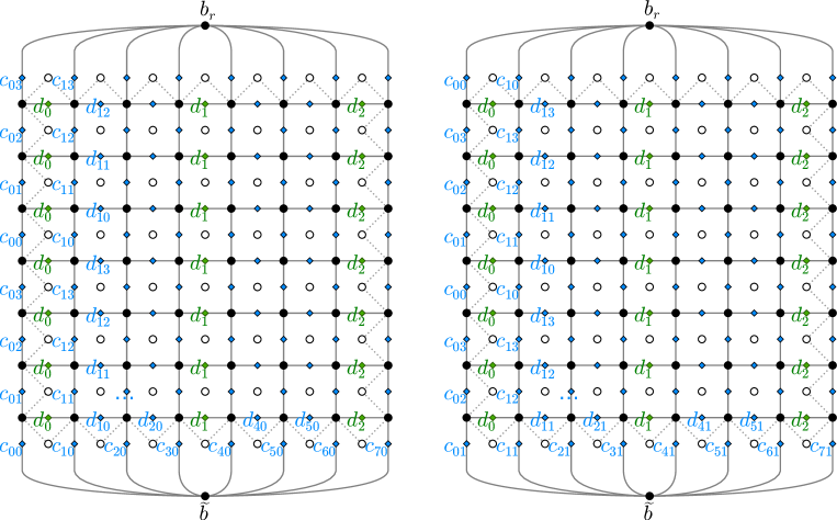
Figure 22: Left: the weights $a$ corresponding to the application of Theorem 5.8. Here $m=4$ and $p=3$, so the Aztec diamond $A_{k}$ has size $k=mp-2p+1=7$; its boundary is shown in dotted lines. The graph $G^{\bullet}$ is shown in solid lines and black dots, recall that its vertices are $\{B,\tilde{b},b_{r}\}$. The weights $(c_{i,j})$ and $(d_{i,j})$ are attached to elements of $F$, or equivalently edges of $G^{\bullet}$, shown as green and blue diamonds. The weights are periodic with period $(0,4)$. In $(d_{i,j})$, constant columns appear every $3$ columns, and correspond to green diamonds. No other periodicity is assumed on the weights. Right: the shifted weights $\tilde{a}$ on the same graph.

Theorem 5.8.

Let $m\geq 2,p\geq 1$, and let $k=mp-2p+1$. Suppose that the weights of the Aztec diamond $A_{k}$ satisfy (5.12). Then the ratio function of oriented dimers associated to face weights $a$ and translated weights $\tilde{a}$ of (5.13) are equal:

$$Y(A_{k},a)=Y(A_{k},\tilde{a}).$$

The proof is more abstract than those of the previous sections. It uses Theorem 5.3, the matrix $C$ defined in Sections 4.2 and the associated matrix $D$ of Section 5.1; but this time, the proof is not based on a combinatorial identification of the ratios of partition functions. A purely combinatorial proof still eludes us.

Proof.

Recall that Theorem 5.3 expresses the ratio function $Y(A_{k},a)$ of oriented dimers using a non-zero vector $v\in\mathbb{C}^{F}$ in the kernel of $D^{T}$, where $D=\begin{pmatrix}C(1)^{B}&C(a)^{B}\end{pmatrix},$ is the matrix obtained from the matrix $C$ by removing the column corresponding to $\tilde{b}$. The proof consists in creating such a vector $v$ that is in addition $(0,m)$-periodic, and using it to prove the invariance result.

For that purpose, we consider a graph $\bar{G^{\bullet}}$ on a cylinder, obtained as a quotient of $G^{\bullet}\setminus\{b_{r},\tilde{b}\}$ by $(0,m)$, see Figure 23. This graph has vertices $\bar{B}$ and edges $\bar{F}$ equipped with weights inherited from that of $G^{\bullet}$. On $\bar{G^{\bullet}}$ we define the analogous operators $\bar{C}(1)^{\bar{B}},\bar{C}(a)^{\bar{B}},$ and $\bar{D}=\begin{pmatrix}\bar{C}(1)^{\bar{B}}&\bar{C}(a)^{\bar{B}}\end{pmatrix}$. Our goal is to find a vector in $\ker\bar{D}^{T}$, and lift it to a vector in $\ker D^{T}$.

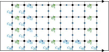
Figure 23: The quotient graph $\bar{G^{\bullet}}$, defined on a cylinder, corresponding to the setting of Figure 22. Constant columns are shown with green diamonds.

We claim that

$$\dim\ker\bar{D}^{T}\geq 1.$$ (5.14)

To show this, let us first compute the dimensions of the initial and target space of $\bar{D}$. Simple counting shows that $2|\bar{B}|=2mk+2m$ and $|\bar{F}|=2mk+m$. Then, applying the rank-nullity theorem to $\bar{D}$ and $\bar{D}^{T}$, we get that the statement (5.14) is equivalent to $\dim\ker\bar{D}\geq 1+2|\bar{B}|-|\bar{F}|=m+1$. Let us find $m+1$ free vectors in $\ker\bar{D}=\ker\begin{pmatrix}\bar{C}(1)^{\bar{B}}&\bar{C}(a)^{\bar{B}}\end{pmatrix}$. Again we are considering these vectors as defined on two copies of $\bar{B}$.

Consider the connected components of black vertices obtained by removing the horizontal edges on the “constant columns” (shown in green in Figure 23). Using the exact value of $k=mp-2p+1$, we get that there are $m$ such connected components. Consider a vector that is equal to $\alpha_{i}$ (resp. $\beta_{i}$) on the whole $i$-th connected component, in the first (resp. second) copy of $\bar{B}$. Then, for any edge in $\bar{F}$ that is not in one of the constant columns, this vector will produce a zero (as $\bar{C}(1)^{\bar{B}}$ outputs the difference of the two values adjacent to $f$, and $\bar{C}(a)^{\bar{B}}$ outputs this difference multiplied by $a_{f}$). So this vector is in $\ker\bar{D}$ iff edges in the constant columns also output zeros, which amounts to

$$\forall i\in\{0,\dots,m-2\},\ \alpha_{i+1}-\alpha_{i}+d_{i}\left(\beta_{i+1}-\beta_{i}\right)=0.$$

This is a system of $m-1$ equation on $2m$ variables $\left(\alpha_{i},\beta_{i}\right)$, so it has rank at most $m-1$, and its kernel has dimension at least $2m-(m-1)=m+1$. It is clear that these $m+1$ free solutions produce $m+1$ free vectors in $\ker\bar{D}$. This proves Equation (5.14).

Therefore, we can fix a nonzero vector $\bar{v}\in\ker\bar{D}^{T}$. Consider the weight-preserving quotient by $(0,m)$, which maps $F$ onto $\bar{F}$. Using this application, we can lift the vector $\bar{v}\in\mathbb{C}^{\bar{F}}$ to a vector $v\in\mathbb{C}^{F}$, by setting the value $v_{f}$ to be $\bar{v}_{\bar{f}}$, for any $f\in F$. The crucial observation is that $v\in\ker D^{T}$. Indeed, for any vertex $b\in B$, the neighbouring elements of $F$ are the same in the initial graph $G^{\bullet}$ as in the quotient graph $\bar{G^{\bullet}}$, so the computation of rows labeled $b$ in the expression $D^{T}v$ is the same as that labeled $\bar{b}$ in $\bar{D}^{T}\bar{v}$. Therefore, by Theorem 5.3,

$$Y(A_{k},a)=-\frac{\sum_{j=0}^{k}c_{j,0}\bar{v}_{j,0}}{\sum_{j=0}^{k}\bar{v}_{j,0}},$$ (5.15)

where $\bar{v}_{j,0}$ is the value of $\bar{v}$ at the element of $\bar{F}$ with weight $c_{j,0}$; note that the indices and the sign have been adapted due to the choice of the position of $\tilde{b}$ in Figure 22.

Now consider the Aztec diamond with shifted weights $\tilde{a}$ (see Figure 22, right). Its quotient graph on the cylinder is exactly the same graph $\bar{G}^{\bullet}$, with the same weights. Therefore we can use the same vector $\bar{v}$ to apply the previous procedure, which gives

$$Y(A_{k},\tilde{a})=-\frac{\sum_{j=0}^{k}c_{j,1}\bar{v}_{j,1}}{\sum_{j=0}^{k}\bar{v}_{j,1}}.$$ (5.16)

Since $\bar{v}\in\ker{\bar{D}^{T}}$, in particular $\bar{v}\in\ker\left(\bar{C}(1)^{\bar{B}}\right)^{T}$. Writing what this means for the $k+1$ elements of $\bar{B}$ shown as the bottom row in Figure 23, and summing all these equations, we get

$$\sum_{j=0}^{k}\bar{v}_{j,0}=\sum_{j=0}^{k}\bar{v}_{j,1}.$$ (5.17)

Doing the same for $\left(\bar{C}(a)^{\bar{B}}\right)^{T}$ gives

$$\sum_{j=0}^{k}c_{j,0}\bar{v}_{j,0}=\sum_{j=0}^{k}c_{j,1}\bar{v}_{j,1}.$$ (5.18)

Using Equations (5.17), (5.18), we get that (5.15), (5.16) are equal. ∎

Remark 5.9.

Note that this generalizes the second result of Theorem 5.4. Nevertheless, we chose a combinatorial approach there, providing an invariance result for the partition function $Z(A_{k},a)$ itself, which is stronger, and cannot be reached by this technique.

5.5 dSKP Devron properties

We finish this section with the proofs of Devron properties as they are stated in the introduction, namely Theorem 1.4, Theorem 1.6 and Corollary 1.5. For this purpose, we go back to the initial convention for indices on the lattice $\mathcal{L}$. We first rephrase Corollary 5.7 in terms of the dSKP solution. Consider again some function $x:\mathcal{L}\to\hat{\mathbb{C}}$ satisfying the dSKP recurrence, the height function $h(i,j)=[i+j]_{2}$, and initial data $(a_{i,j})=(x(i,j,h(i,j)))$, with no periodicity assumption.

Corollary 5.10.

Suppose that the initial data are such that for some $d\in\hat{\mathbb{C}}$, for all $(i,j)\in\mathbb{Z}^{2}$ such that $[i+j]_{2}=0$, $a_{i,j}=d$. Let $(i,j,k)\in\mathcal{L}$ with $k\geq 1$. Consider the matrix $N=\left(N_{i^{\prime},j^{\prime}}\right)_{0\leq i^{\prime},j^{\prime}\leq k-1}$ with entries

$$N_{i^{\prime},j^{\prime}}=\left(a_{i-i^{\prime}+j^{\prime},j+k-1-i^{\prime}-j^{\prime}}-d\right)^{-1}.$$

Then

$$x(i,j,k)=d+\sum_{0\leq i^{\prime},j^{\prime}\leq k-1}\left(N^{-1}\right)_{i^{\prime},j^{\prime}},$$

where the sum is over entries of the inverse matrix $N^{-1}$.

Proof.

With the stated hypothesis, via Theorem 3.4 as in Example 3.5, the value of $x(i,j,k)$ is $Y(A_{k-1},a)$ for Aztec diamond of size $k-1$, with the central face labeled $a_{i,j}$. This Aztec diamond has face weights as in Corollary 5.7. Rewriting the matrix $N$ in the original coordinate system gives the result. ∎

Proof of Theorem 1.4.

We use Corollary 5.10. In the lattice $\mathcal{L}$, going from $(i,j,m)$ to $(i+1,j+1,m)$ changes the matrix $N$ simply by a cyclic permutation of the rows, which does not change the value of the sum of coefficients of $N^{-1}$. Therefore $x(i,j,m)=x(i+1,j+1,m)$, and similarly $x(i,j,m)=x(i+1,j-1,m)$, which proves that this value is independent of $i,j$ as long as $(i,j,m)\in\mathcal{L}$. ∎

Proof of Theorem 1.6.

The argument is almost the same, except now the weights on the corresponding Aztec diamond of size $k-1=(m-2)p+1$ satisfy the hypothesis of Theorem 5.8, in particular the fact that $[i-j-mp]_{2p}=0$ translates into the fact that constant columns appear at the leftmost and rightmost columns of inner faces, as in (5.12) and Figure 22. Going in $\mathcal{L}$ from $(i,j,k)$ to $(i+1,j+1,k)$ has the effect of changing the Aztec diamond weights $a$ into $\tilde{a}$, so the result is a rephrasing of Theorem 5.8. ∎

For the proof of Corollary 1.5, we need the following basic lemma:

Lemma 5.11.

Let $N$ be an invertible $m\times m$ matrix. Suppose that there is a $\lambda\in\mathbb{C}^{*}$ such that for all $i,$ $\sum_{j}N_{ij}=\lambda$. Then $\sum_{i,j}(N^{-1})_{ij}=n\lambda^{-1}$.

Proof.

The vector $o\in\mathbb{C}^{m}$ with $o_{i}=1$ for all $i$ is clearly an eigenvector of $N$ for the eigenvalue $\lambda$. Therefore $\lambda^{-1}$ is an eigenvalue to eigenvector $o$ for the inverse matrix $N^{-1}$. Thus

$$\sum_{i,j}(N^{-1})_{ij}=o^{T}M^{-1}o=o^{T}\lambda^{-1}o=m\lambda^{-1}.$$

∎

Proof of Corollary 1.5.

For $m$-Dodgson initial conditions, the value of $x(i,j,m)$ whenever $(i,j,m)\in\mathcal{L}$ is given by Corollary 5.10. Under the condition $a_{i,j}=a_{i+p+1,j-p+1}$, note that the successive rows of $N$ contain the same variables, shifted by $p$ from one row to the next. Therefore $N$ satisfies the conditions of Lemma 5.11 with $\lambda$ being the sum of the $\frac{1}{a-d}$ on one row of $N$. ∎

Finally, we describe how these singularities occur for initial data with two different periodicities. For a vector $(s,t)$ in $\mathbb{Z}^{2}$ with $[s+t]_{2}=0$, we say that the initial data is $(s,t)$-periodic if $a_{i,j}=a_{i+s,j+t}$ for all $(i,j)\in\mathbb{Z}^{2}$. The following describes how many steps one has to go until singularities reoccur when initial conditions have two such periodicities.

Corollary 5.12.

Let $(s,t)$ and $(u,v)$ be two noncolinear vectors in $\mathbb{Z}^{2}$, with $[s+t]_{2}=[u+v]_{2}=0$. Suppose that the initial condition is both $(s,t)$ and $(u,v)$ periodic. Let $g=\gcd(s-t,u-v)$, and $\mathcal{A}=|sv-tu|$.

• If the initial data is such that for all $(i,j)\in\mathbb{Z}^{2}$ with $[i+j]_{2}=0$,

  $$a(i,j)=a(i+1,j+1),$$

  then for $k=\frac{\mathcal{A}}{g}$ the same is true at height $k$. More precisely,

  $$\forall i,j\text{ s.t. }(i,j,k)\in\mathcal{L},\ x(i,j,k)=x(i+1,j+1,k).$$

• If the initial data is such that

  $$\forall i\in\mathbb{Z},a_{i,i}=a_{i+1,i+1},$$

  then let $k=\frac{\mathcal{A}}{2}-g+2$. After $k-1$ iterations of the dSKP recurrence, the values of $x$ have $\frac{g}{2}$-periodic constant columns. More precisely, for all $i,j$ such that $\left[i-j-\frac{\mathcal{A}}{2}\right]_{\frac{g}{2}}=0$,

  $$x(i,j,k)=x(i+1,j+1,k).$$

Proof.

We are relating the initial data $a$ to the hypothesis of Theorem 1.6. First we are looking for $m$ such that $a$ is $m$-simply periodic. This is equivalent to

$$(m,m)\in\mathbb{Z}(s,t)+\mathbb{Z}(u,v).$$

Classical arithmetic computations show that the smallest positive such $m$ is $\frac{\mathcal{A}}{g}$. In the first point, this shows that the initial data is $(m,1)$-Devron, and we get the result by applying Theorem 1.6.

In the second point, we want to find $p$ such that the constant “column” $(a_{i,i})_{i\in\mathbb{Z}}$ repeats every $p$ even column. Since the initial data is $(s,t)$-periodic, this is true for $p_{1}=\frac{s-t}{2}$, and similarly for $p_{2}=\frac{u-v}{2}$, so the smallest positive $p$ is $\gcd\left(p_{1},p_{2}\right)=\frac{g}{2}$. For these values of $m$ and $p$, the initial data is $(m,p)$-Devron, and we apply Theorem 1.6. ∎

6 Limit shapes

Suppose that $x:\mathcal{L}\to\hat{\mathbb{C}}$ satisfies the dSKP recurrence. Let $h(i,j)=[i+j]_{2}$ then for any $p\in\mathcal{U}_{h}$, we may consider $x(p)$ as a function of the $(a_{i,j})=(x(i,j,h(i,j)))$, given by Theorem 3.4 We are interested in the effect of the initial condition at $(0,0,0)$ on the value of $x_{p}$. Let

$$\rho(i,j,k)=\dfrac{\partial x(i,j,k)}{\partial x(0,0,0)}.$$ (6.1)

We are looking for the order of magnitude of $\rho(i,j,k)$ when $k\to\infty$ and $i/k,j/k$ both converge to some constants. This behaviour is made explicit in the forthcoming Proposition 6.1, when the derivative (6.1) is evaluated at specific dSKP solutions of Example 2.4. By a slight abuse of notation, for $x,y\in\mathbb{R}$, we denote $\rho(xk,yk,k):=\rho\left(\lfloor xk\rfloor,\lfloor yk\rfloor,k\right)$.

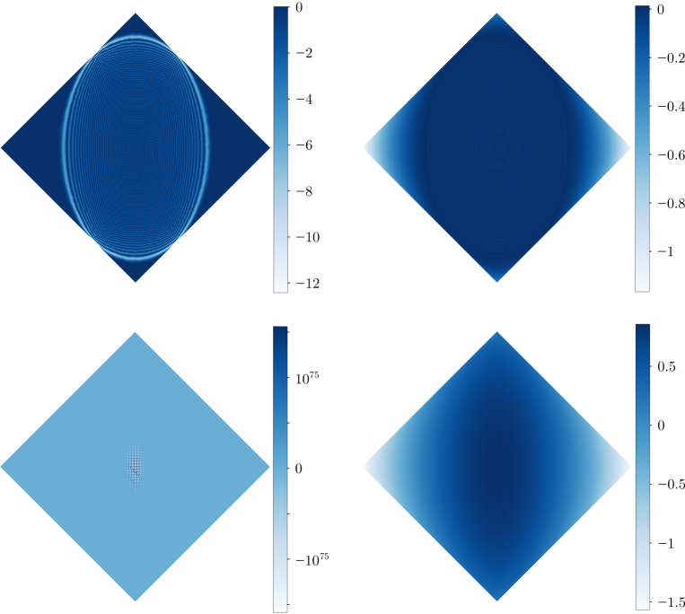
Figure 24: Values of $k\rho(i,j,k)$ (left) and $\frac{\log|k\rho(i,j,k)|}{k}$ (right) for $k=200$, evaluated at the solution $x(i,j,k)=ia+jb+kc+d$, with $q:=\frac{c^{2}-b^{2}}{a^{2}-b^{2}}=0.7$ (top) and $q=1.2$ (bottom).

The identification of the asymptotic behaviour of $\rho(xk,yk,k)$ when $k\to\infty$ follows the plan of [DFSG14, Section 2.3], that treats the analogous problem in the dKP relation. In fact both cases produce almost the same generating functions, however we use different references to deduce the asymptotics. We mainly identify the generating functions with that of [BBC⁺17] (although they were probably known way before, see references therein), from which point the asymptotic behaviour can be recovered almost directly from [CEP⁺96].

Proposition 6.1.

Let $a,b,c,d\in\mathbb{R}$. Let $q=\frac{c^{2}-b^{2}}{a^{2}-b^{2}}$. Consider the partial derivatives $\rho(i,j,k)$ evaluated at $x(i,j,k)=ia+jb+kc+d$. Let $x,y\in\mathbb{R}$ be such that $|x+y|<1$ and $|x-y|<1$.

1. If $q\in(0,1)$,

   1. for all $x,y$ such that $\frac{x^{2}}{1-q}+\frac{y^{2}}{q}<1$ and $(kx,ky,k)\in\mathcal{L}$,

      $$\rho(xk,yk,k)=\frac{2\cos^{2}(\Phi_{q}(xk,yk,k))}{k\pi\sqrt{q(1-q)-qx^{2}-(1-q)y^{2}}}\left(1+O\left(k^{-1}\right)\right)),$$ (6.2)

      where the function $\Phi_{q}:\mathcal{L}\to\mathbb{R}$ can be determined explicitly.

   2. for all $x,y$ such that $\frac{x^{2}}{1-q}+\frac{y^{2}}{q}>1$,

      $$\rho(xk,yk,k)=\pm\frac{c_{q}(x,y)}{k}\exp(\xi_{q}(x,y)k)\ \left(1+o(1)\right),$$ (6.3)

      where $\xi_{q}(x,y)<0$ and $c_{q}(x,y)\in\mathbb{R}$ can be determined explicitly.

2. If $q\in(-\infty,0)\cup(1,\infty)$, for all $x,y$,

   $$\rho(xk,yk,k)=\pm\frac{c_{q}(x,y)}{k}\exp(\xi_{q}(x,y)k)\ \left(1+o(1)\right),$$ (6.4)

   where $\xi_{q}(x,y)\in\mathbb{R}$ and $c_{q}(x,y)\in\mathbb{R}$ can be determined explicitly. Moreover, $\xi_{q}(x,y)>0$ in a neighbourhood of $(0,0)$.

Proof.

Let us differentiate (2.1) with respect to $x(0,0,0)$. This gives the following, evaluated at any $p=(i,j,k)\in\mathbb{Z}^{3}\setminus\mathcal{L}$ with $k\geq 1$:

$$\begin{split}0=&\rho_{-e_{0}}\frac{x_{e_{2}}-x_{-e_{1}}}{(x_{-e_{0}}-x_{-e_{1}})(x_{e_{2}}-x_{-e_{0}})}+\rho_{-e_{1}}\frac{x_{-e_{2}}-x_{-e_{0}}}{(x_{-e_{1}}-x_{-e_{0}})(x_{-e_{2}}-x_{-e_{1}})}\\ &+\rho_{-e_{2}}\frac{x_{-e_{1}}-x_{e_{0}}}{(x_{-e_{2}}-x_{e_{0}})(x_{-e_{1}}-x_{-e_{2}})}+\rho_{e_{0}}\frac{x_{e_{1}}-x_{-e_{2}}}{(x_{e_{0}}-x_{-e_{2}})(x_{e_{1}}-x_{e_{0}})}\\ &+\rho_{e_{1}}\frac{x_{e_{0}}-x_{e_{2}}}{(x_{e_{1}}-x_{e_{2}})(x_{e_{0}}-x_{e_{1}})}+\rho_{e_{2}}\frac{x_{-e_{0}}-x_{e_{1}}}{(x_{e_{2}}-x_{e_{1}})(x_{-e_{0}}-x_{e_{2}})}.\end{split}$$ (6.5)

After evaluating at $x(i,j,k)=ia+jb+kc+d$, the relation becomes

$$\rho_{-e_{2}}+\rho_{e_{2}}=q\left(\rho_{-e_{0}}+\rho_{e_{0}}\right)+(1-q)\left(\rho_{-e_{1}}+\rho_{e_{1}}\right),$$ (6.6)

where $q=\frac{c^{2}-b^{2}}{a^{2}-b^{2}}$. From this linear relation, and handling separately the case of $\rho(i,j,k)$ with $k=0$ or $1$, we deduce the generating function:

$$\begin{split}F(u,v,t):=&\sum_{\begin{subarray}{c}(i,j,k)\in\mathcal{L},\\ k\geq 0\end{subarray}}\rho(i,j,k)u^{i}v^{j}t^{k}\\ =&1-\frac{t^{2}}{1+t^{2}-qt(x+x^{-1})-(1-q)t(y+y^{-1})}.\end{split}$$ (6.7)

This is directly related to the generating function of the creation rate of the Aztec diamond that can be found in [BBC⁺17, Remark 23] for $\lambda=\frac{1-q}{q}$. By this identification and [BBC⁺17, Proposition 21], we get

$$\forall(i,j,k)\in\mathcal{L},k\geq 1,\ \rho(i,j,k)=-(1-q)^{k-2}C_{q}(A,B,k-2)C_{q}(B,A,k-2),$$ (6.8)

where $C_{q}(A,B,n)$ is the coefficient of $z^{A}$ in $(1-z)^{B}\left(1+\frac{q}{1-q}z\right)^{n-B}$, and $A=\frac{k-2-i-j}{2}$, $B=\frac{k-2+i-j}{2}$.

The asymptotics of $C_{q}(A,B,n)$ when $n\to\infty$ and $A,B$ are proportional to $n$ can be analyzed by the saddle point method (see e.g. [FS09, Section VIII]). In case 1a, this is done in [CEP⁺96, Proposition 24], which gives the result after changing variables back to our setting. Case 1b follows closely the proof of [CEP⁺96, Proposition 8], the main difference being that we apply the full saddle-point method instead of just looking for an upper bound; therefore, we only give details for case 2 below.

Let us suppose that $q>1$, the case $q<0$ being almost identical. We are looking for the asymptotics of $C_{q}(A,B,k-2)$, when $k\to\infty$ and $A\sim\frac{1-x-y}{2}k,B\sim\frac{1+x-y}{2}k$. Performing a contour integral of

$$f(z)=\frac{1}{2i\pi}(1-z)^{B}\left(1-\frac{q}{q-1}z\right)^{k-2-B}z^{-A-1},$$ (6.9)

around $0$ gives $C_{q}(A,B,k-2)$. It is easy to check that $f$ has critical points at $1,\frac{q-1}{q}$, and two other points that are both real. Up to $O(k^{-1})$, these two points are

$$z_{\pm}=\frac{(q-1)x+qy\pm\sqrt{(1-q)x^{2}+qy^{2}-q(1-q)}}{q(x+y+1)}.$$ (6.10)

In fact the points $1,\frac{q-1}{q}$ are minima of $|f|$, while $z_{\pm}$ are saddle points. Then, studying $|f|$ on the real axis, we get that $z_{-}<0<\frac{q-1}{q}<z_{+}<1$. From this observation, we can chose a contour of integration going through $z_{-}$, such that $z_{-}$ is the position of a maximum of $|f|$ on this contour. Around the saddle-point $z_{-}$, $f(z)$ can be written as $f(z)=\pm\frac{1}{2i\pi}\exp\left(kg(z)+O(1)\right)$, where

$$g(z)=\frac{1+x-y}{2}\log(1-z)+\frac{1-x+y}{2}\log\left(1-\frac{q}{q-1}z\right)-\frac{1-x-y}{2}\log(-z),$$ (6.11)

taking $\log$ to be the principal value of the complex logarithm.

The setup of the saddle-point method is complete, and it gives

$$C_{q}(A,B,k-2)=\pm\frac{1}{\sqrt{2\pi|g^{\prime\prime}(z_{-})|k}}\exp\left[g(z_{-})k\right]\ \left(1+o(1)\right).$$ (6.12)

Combining (6.12) and (6.8) yields the asymptotic for $\rho(xk,yk,k)$. Moreover, it shows that $c_{q},\xi_{q}$ are explicit and continuous functions, so to get the last claim, it suffices to show that $\xi_{q}(0,0)>0$. For $x=y=0$, an explicit computation shows that $z_{-}=-\sqrt{\frac{q-1}{q}},$ then $g(z_{-})=\log\left(1+\sqrt{\frac{q}{q-1}}\right),$ and then $\xi_{q}(0,0)=2\log\left(\sqrt{q}+\sqrt{q-1}\right)>0$.

∎

Remark 6.2.

The case $q\in(0,1)$ exhibits a phenomenon commonly known as a limit shape. The decay of $\rho(xk,yk,k)$ to zero is either of order $k^{-1}$ inside the arctic ellipse $\frac{x^{2}}{1-q}+\frac{y^{2}}{q}=1$, or exponential outside the ellipse. By contrast, for $q\in(-\infty,0)\cup(1,\infty)$, the derivative $\rho(xk,yk,k)$ always has an exponential behaviour, with a positive rate on some neighbourhood of $(0,0)$ (and for some values of $q$, it seems, for all possible $x,y$). This is indicative of a chaotic behaviour of the dSKP recurrence. Proposition 6.1, although restricted to very special initial conditions, gives quantitative estimates for such a chaotic behaviour.

Remark 6.3.

In the case of the other special solution of Example 2.4, $x(i,j,k)=a^{i}b^{j}c^{k}d$, relation (6.6) is satisfied for the following logarithmic derivative:

$$\tilde{\rho}(i,j,k):=\frac{x(0,0,0)}{x(i,j,k)}\dfrac{\partial x(i,j,k)}{\partial x(0,0,0)},$$ (6.13)

with $q=\frac{a(c-b)(bc-1)}{c(a-b)(ab-1)}$. The rest of the proof is unchanged, so Proposition 6.1 applies to $\tilde{\rho}(i,j,k)$, governed by that value of $q$. Of course, using the asymptotics of $\tilde{\rho}(i,j,k)$ and the explicit value of $x(i,j,k)$, one also gets the asymptotics of $\rho(i,j,k)$ in that case. On the other hand, for other recurrences where there is a probabilistic interpretation such as dKP, $\tilde{\rho}$ is a commonly considered observable that carries a statistical meaning sufficient to describe the existence of a limit shape with high probability; see again [DFSG14].

7 The other consistent equations of octahedron type

In [ABS12], Adler, Bobenko and Suris introduce the notion of multidimensional consistency for system of equations on the root lattice $Q(A_{3})$, see Remark 2.1. They show that up to a set of transformations called admissible, any such system can be transformed into a system belonging to a finite list $\{\chi_{1},\chi_{2},\chi_{3},\chi_{4},\chi_{5}\}$. By changing variables into the lattice $\mathcal{L}$ using Remark 2.1, $\chi_{1}$ corresponds to the dKP recurrence (Definition 2.5), and $\chi_{2}$ to the dSKP recurrence (Definition 2.2). We now turn our attention to the last three systems. Translated into $\mathcal{L}$, they give the following definitions:

Definition 7.1.

A function $x:\mathcal{L}\rightarrow\hat{\mathbb{C}}$ satisfies the $\chi_{3}$, resp. $\chi_{4},\chi_{5}$ recurrence if

$$\chi_{3}:\ \ (x_{e_{3}}-x_{-e_{2}})x_{-e_{1}}+(x_{-e_{2}}-x_{e_{1}})x_{-e_{3}}+(x_{e_{1}}-x_{e_{3}})x_{e_{2}}=0,$$

$$\text{resp. }\chi_{4}:\ \ \frac{x_{e_{3}}-x_{-e_{2}}}{x_{-e_{1}}}+\frac{x_{-e_{2}}-x_{e_{1}}}{x_{-e_{3}}}+\frac{x_{e_{1}}-x_{e_{3}}}{x_{e_{2}}}=0,$$

$$\text{resp. }\chi_{5}:\ \ \frac{x_{e_{3}}-x_{e_{1}}}{x_{e_{2}}}=x_{-e_{2}}\left(\frac{1}{x_{-e_{3}}}-\frac{1}{x_{-e_{1}}}\right),$$

holds evaluated at any $p$ of $\mathbb{Z}^{3}\setminus\mathcal{L}$.

For $\varepsilon>0$ and a rational fraction $Q(\varepsilon)$, we denote by $\operatorname{lc}_{\epsilon}Q(\varepsilon)$ the leading coefficient in $\varepsilon$ in the asymptotic development of $Q(\varepsilon)$ at $\varepsilon\to 0$. Solutions of the $\chi_{3},\chi_{4}$ and $\chi_{5}$ recurrences can be deduced from that of dSKP by taking successive leading terms in $\varepsilon$ limits of the initial conditions:

Theorem 7.2.

Let $x:\mathcal{L}\rightarrow\hat{\mathbb{C}}$ be a function that satisfies the $\chi_{3}$, resp. $\chi_{4},\chi_{5}$ recurrence. Let $h$ be a height function, and $\mathcal{I},\mathcal{U}$ be defined as in Equations (2.2), (2.3). Let $(a_{i,j})=(x(i,j,h(i,j)))$ be the initial data indexed by points of $\mathcal{I}$. For $\varepsilon,\delta,\rho>0$, let

$$\begin{split}a_{i,j}^{\epsilon,\rho}&=(1+\rho\epsilon^{i-j+k}a_{i,j}),\\ a_{i,j}^{\epsilon}&=\epsilon^{i-j+k}a_{i,j},\\ a_{i,j}^{\epsilon,\delta}&=\epsilon^{i-j+k}\delta^{i+j+k}a_{i,j}.\end{split}$$ (7.1)

Then for every point $p$ of $\mathcal{U}$,

$$\begin{split}\chi_{3}:\ \ x(p)&=\operatorname{lc}_{\rho}\left(\operatorname{lc}_{\epsilon}Y(G_{p},a^{\epsilon,\rho})-1\right),\\ \text{resp. }\chi_{4}:\ \ x(p)&=\operatorname{lc}_{\epsilon}Y(G_{p},a^{\epsilon}),\\ \text{resp. }\chi_{5}:\ \ x(p)&=\operatorname{lc}_{\delta}\left(\operatorname{lc}_{\epsilon}Y(G_{p},a^{\epsilon,\delta})\right),\end{split}$$ (7.2)

where $G_{p}$ is the crosses and wrenches graph corresponding to $p$.

Proof.

We use [ABS12, Remark 3]. Changing variables using Remark 2.1, it states that if one starts with the initial data $a^{\varepsilon}_{i,j}$ and applies the dSKP recurrence, then the leading coefficient in $\varepsilon$ satisfies the $\chi_{4}$ recurrence. More precisely, it can be checked directly by induction that if $x$ is the solution of the $\chi_{4}$ recurrence with initial data $a$, and $x^{\varepsilon}$ is the solution of the dSKP recurrence with initial data $a^{\varepsilon}$, then for any $p=(i,j,k)$, $x^{\varepsilon}(p)=\varepsilon^{i-j+k}\left(x(p)+O(\varepsilon^{2})\right)$. Therefore, the formula for $x(p)$ in the $\chi_{4}$ case is a consequence of Theorem 3.4.

The $\chi_{5}$ and $\chi_{3}$ cases are then limits from the $\chi_{4}$ solution itself. For $\chi_{5}$, it can also be deduced from [ABS12, Remark 3], where the expression as a $\delta$ limit from $\chi_{4}$ is stated; the proof is identical to the previous one. For $\chi_{3}$, the $\rho$ limit seems to be new. The proof consists in checking that if $x$ is the solution of the $\chi_{3}$ recurrence with initial data $b$, and if $x^{\rho}$ is the solution of the $\chi_{4}$ recurrence with initial data $1+\rho b$, then for any $p,x^{\rho}(p)=1+\rho x(p)+O(\rho^{2})$. ∎

	Aztec diamond size	$1$	$2$	$3$	$4$
$\chi_{2}$	numerator	$6$	$220$	$49224$	?
	denominator	$6$	$220$	$49224$	?
$\chi_{3}$	numerator	$4$	$30$	$680$	$45188$
	denominator	$2$	$14$	$300$	$19044$
$\chi_{4}$	numerator	$4$	$56$	$2656$	?
	denominator	$2$	$14$	$328$	?
$\chi_{5}$	numerator	$3$	$23$	$433$	$19705$
	denominator	$1$	$3$	$23$	$433$

Table 1: Number of contributing configurations of Aztec diamonds of small size.

In fact, at least in the case where the crosses and wrenches graph is the Aztec diamond (as in Example 3.5), it is relatively easy to describe exactly the combinatorics of configurations that appear in the leading terms of Theorem 7.2, at least in the $\chi_{4}$ and $\chi_{5}$ cases. We describe these configurations here. We leave the $\chi_{3}$ case as an open problem, as well as the case of more generic height functions.

Recall that for the height function $h(i,j)=[i+j]_{2}$, the solution of the dSKP recurrence at $p=(i,j,k+1)$ is expressed as $Y(A_{k},a)$ for an Aztec diamond of size $k$. By Equation (3.3) and Corollary 5.1, this solution may be expressed as

$$Y(A_{k},a)=\biggl{(}\,\prod_{f\in F_{p}}a_{f}\biggr{)}\frac{Z(A_{k},a^{-1},\varphi)}{Z(A_{k},a,\varphi)}=\frac{\sum_{(\mathsf{T},\mathsf{F})\in\mathscr{F}}\operatorname{sign}(\mathsf{T},\mathsf{F})\prod_{\vec{e}\in\mathsf{T}}a_{f_{\vec{e}}}}{\sum_{(\mathsf{T},\mathsf{F})\in\mathscr{F}}\operatorname{sign}(\mathsf{T},\mathsf{F})\prod_{\vec{e}\in\mathsf{F}}a_{f_{\vec{e}}}},$$

where the sums are over pairs of complementary trees/forests on $G^{\bullet}$, with a one-to-one correspondence between configurations and monomials. To identify the terms that contribute in the $\chi_{4}$ case, let us apply the previous equation at $a_{i,j}^{\epsilon}=\epsilon^{i-j+k}a_{i,j}$, and look for the terms that minimize the $\epsilon$ exponent. We do this first in the denominator, so we are looking for configurations $(\mathsf{T},\mathsf{F})$ such that the $\epsilon$ exponent of variables in $\mathsf{F}$ is minimal. Recall that in the forest $\mathsf{F}$, every black vertex has one outgoing edge. Looking at the exponents of $\epsilon$ around a black vertex in Figure 25, top left, this exponent is minimal if the forest never has an edge oriented towards the South-East. We claim that there exist such configurations, an example is displayed in Figure 25, top left. Thus, the previous constraint completely characterize those configurations that appear in the denominator of the solution of the $\chi_{4}$ recurrence.

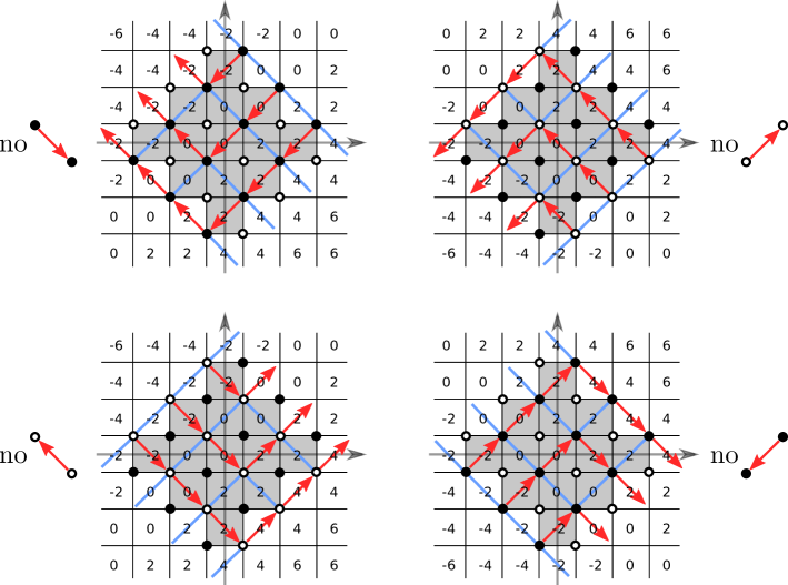
Figure 25: Example configurations contributing to the solutions of the $\chi_{4}$ and $\chi_{5}$ recurrence, for the initial data of Example 3.5. Top left: the numbers indicate the exponent of $\epsilon$ in $a^{\epsilon}_{i,j}$; a tree/forest configuration on $G^{\bullet}$ is shown, with the forest shown in red and oriented, and vertices $b_{r},\tilde{b}$ thought of as being “at infinity”; this configuration minimizes the $\epsilon$ exponent, so it contributes to the denominator of the $\chi_{4}$ solution. Top right: the exponent of $\delta$ in $a^{\epsilon,\delta}_{i,j}$; the tree/forest configuration on $G^{\circ}$ minimizes the $\delta$ exponent, and corresponds to the top left configuration via the bijection; hence it also contributes to the denominator for $\chi_{5}$. Bottom: similarly, a configuration shown either on $G^{\circ}$ or on $G^{\bullet}$, such that the forest maximizes the $\epsilon$ and $\delta$ exponents, hence contributing to the numerator of both $\chi_{4}$ and $\chi_{5}$.

For the numerator, we have to minimize the $\epsilon$ exponent in $\mathsf{T}$ instead, so have to maximize it in $\mathsf{F}$. Consider the graph $G^{\circ}$ analogous to $G^{\bullet}$ for white vertices. There is a bijection between pairs of complementary trees/forests on $G^{\bullet}$ and those on $G^{\circ}$, obtained by replacing every black diagonal in $\mathsf{F}$ into the corresponding white diagonal. Therefore, we may consider configurations on $G^{\circ}$. On that graph, the same argument shows that the $\epsilon$ exponent in $\mathsf{F}$ is maximal when there is no edge oriented towards the North-West. An example is shown in Figure 25, bottom left.

For the $\chi_{5}$ case, we now have to minimize both the $\epsilon$ exponent and the $\delta$ exponent. Similar considerations show that contributing configurations for the denominator are those for which in $G^{\bullet}$, $\mathsf{F}$ has no South-East going edge (to minimize the $\epsilon$ exponent as before), and for the corresponding forest on $G^{\circ}$, the forest has no North-East going edge (to minimize the $\delta$ exponent). The previous example satisfies both these constraint, see Figure 25, top right. In the numerator, the contributing configurations are such that in the forest on $G^{\circ}$ there is no North-West going edge, and in the corresponding forest on $G^{\bullet}$ there is no South-West going edge, see Figure 25, bottom right.

As for the $\chi_{3}$ case, note that we would have to consider the configurations coming from $\chi_{4}$ and write their weight in variables $1+\rho a_{i,j,k}$, in order to expand each weight and find the leading coefficient in $\rho$. Computing these by hand for small values of $k$, it turns out that both in the numerator and denominator, the coefficient in $\rho^{0}$ vanishes. We were not able to find a simple combinatorial identification for the coefficients in $\rho^{1}$ (which a priori may come from the expansion of several of the $\chi_{4}$ configurations).

The number of contributing configurations for the first Aztec diamond sizes (i.e. the number of monomials in the corresponding solution of the $\chi_{i}$ recurrences) that we were able to compute are given in Table 1. For $\chi_{5}$, it seems that there are as many monomials in the numerator for $A_{k}$ as in the denominator for $A_{k+1}$, but we do not see a simple explanation for this pattern, and we do not know if it continues.

References

- [ABS12] Vsevolod E. Adler, Alexander I. Bobenko, and Yuri B. Suris. Classification of Integrable Discrete Equations of Octahedron Type. International Mathematics Research Notices, 2012(8):1822–1889, 01 2012.
- [AdTM22] Niklas C. Affolter, Béatrice de Tilière, and Paul Melotti. The Schwarzian octahedron recurrence (dSKP equation) II: geometric systems. 2022. Preprint on arXiv.
- [Aff21] Niklas C. Affolter. Miquel dynamics, Clifford lattices and the Dimer model. Letters in Mathematical Physics, 111:1–23, 2021.
- [BBC+17] Cédric Boutillier, Jérémie Bouttier, Guillaume Chapuy, Sylvie Corteel, and Sanjay Ramassamy. Dimers on rail yard graphs. Annales de l’Institut Henri Poincaré D, 4(4):479–539, 2017.
- [BK98a] Leonid V. Bogdanov and Boris G. Konopelchenko. Analytic-bilinear approach to integrable hierarchies. I. Generalized KP hierarchy. Journal of Mathematical Physics, 39(9):4683–4700, 1998.
- [BK98b] Leonid V. Bogdanov and Boris G. Konopelchenko. Analytic-bilinear approach to integrable hierarchies. II. Multicomponent KP and 2D Toda lattice hierarchies. Journal of Mathematical Physics, 39(9):4701–4728, 1998.
- [BV99] Marc P. Bellon and Claude-Michel Viallet. Algebraic entropy. Communications in mathematical physics, 204(2):425–437, 1999.
- [CEP+96] Henry Cohn, Noam Elkies, James G. Propp, et al. Local statistics for random domino tilings of the aztec diamond. Duke Mathematical Journal, 85(1):117–166, 1996.
- [Ciu03] Mihai Ciucu. Perfect matchings and perfect powers. Journal of Algebraic Combinatorics, 17(3):335–375, 2003.
- [CLR20] Dmitry Chelkak, Benoît Laslier, and Marianna Russkikh. Dimer model and holomorphic functions on t-embeddings of planar graphs, 2020. Preprint, arXiv:2001.11871.
- [CS04] Gabriel D. Carroll and David E Speyer. The cube recurrence. the electronic journal of combinatorics, 11(R73):1, 2004.
- [DFSG14] Philippe Di Francesco and Rodrigo Soto-Garrido. Arctic curves of the octahedron equation. Journal of Physics A: Mathematical and Theoretical, 47(28):285204, 2014.
- [Dod67] Charles L. Dodgson. IV. Condensation of determinants, being a new and brief method for computing their arithmetical values. Proceedings of the Royal Society of London, (15):150–155, 1867.
- [FS09] Philippe Flajolet and Robert Sedgewick. Analytic Combinatorics. Cambridge University Press, 2009.
- [Geo21] Terrence George. Grove arctic curves from periodic cluster modular transformations. International Mathematics Research Notices, 2021(20):15301–15336, 2021.
- [Gli15] Max Glick. The Devron property. Journal of Geometry and Physics, 87:161–189, 2015.
- [Hir81] Ryogo Hirota. Discrete analogue of a generalized Toda equation. Journal of the Physical Society of Japan, 50(11):3785–3791, 1981.
- [Kas61] Pieter W. Kasteleyn. The statistics of dimers on a lattice : I. The number of dimer arrangements on a quadratic lattice. Physica, 27:1209–1225, December 1961.
- [Kas67] Pieter W. Kasteleyn. Graph theory and crystal physics. In Graph Theory and Theoretical Physics, pages 43–110. Academic Press, London, 1967.
- [KLRR18] Richard W. Kenyon, Wai Yeung Lam, Sanjay Ramassamy, and Marianna Russkikh. Dimers and Circle patterns, 10 2018. Preprint on arXiv:1810.05616.
- [KP16] Richard W. Kenyon and Robin Pemantle. Double-dimers, the ising model and the hexahedron recurrence. Journal of Combinatorial Theory, Series A, 137:27–63, 2016.
- [KPW00] Richard W. Kenyon, James G. Propp, and David B. Wilson. Trees and matchings. Electron. J. Combin, 7(1):R25, 2000.
- [KS02] Boris G. Konopelchenko and Wolfgang K. Schief. Menelaus’ theorem, Clifford configurations and inversive geometry of the Schwarzian KP hierarchy. Journal of Physics A: Mathematical and General, 35(29):6125–6144, 07 2002.
- [Mel18] Paul Melotti. The free-fermionic loop model, double dimers and Kashaev’s recurrence. Journal of Combinatorial Theory, Series A, 158:407–448, 2018.
- [Per69] Jerome K. Percus. One More Technique for the Dimer Problem. J. Math. Phys., 10(10):1881–1884, 1969.
- [Pro03] James G. Propp. Generalized domino-shuffling. Theor. Comput. Sci., 303:267–301, 2003.
- [PS05] T. Kyle Petersen and David E Speyer. An arctic circle theorem for groves. Journal of Combinatorial Theory, Series A, 111(1):137–164, 2005.
- [RG11] Jürgen Richter-Gebert. Perspectives on Projective Geometry: A Guided Tour Through Real and Complex Geometry. Springer Publishing Company, Incorporated, 1st edition, 2011.
- [Spe07] David E Speyer. Perfect matchings and the octahedron recurrence. Journal of Algebraic Combinatorics, 25(3):309–348, 2007.
- [Tem74] Harold N. V. Temperley. In Combinatorics: Proceedings of the British combinatorial conference 1973. page 202–204, 1974.
- [TF61] Harold N. V. Temperley and Michael E. Fisher. Dimer problem in statistical mechanics – an exact result. The Philosophical Magazine: A Journal of Theoretical Experimental and Applied Physics, 6(68):1061–1063, 1961.