Rapid-flooding Time Synchronization
for Large-scale Wireless Sensor Networks

Abstract

Accurate and fast-convergent time synchronization is very important for wireless sensor networks. The flooding time synchronization converges fast, but its transmission delay and by-hop error accumulation seriously reduce the synchronization accuracy. In this paper, a rapid-flooding multiple one-way broadcast time-synchronization (RMTS) protocol for large-scale wireless sensor networks is proposed. To minimize the by-hop error accumulation, the RMTS uses maximum likelihood estimations for clock skew estimation and clock offset estimation, and quickly shares the estimations among the networks. As a result, the synchronization error resulting from delays is greatly reduced, while faster convergence and higher-accuracy synchronization is achieved. Extensive experimental results demonstrate that, even over 24-hops networks, the RMTS is able to build accurate synchronization at the third synchronization period, and moreover, the by-hop error accumulation is slower when the network diameter increases.

I Introduction

Time synchronization is very important to wireless sensor network (WSN) applications, e.g., data acquisition [1, 2], low power [3, TII_7], location services [4, 5], security [6, TII_6], networked control [9, 10], industrial WSNs [11, 12], and smart grid measurement [13, 14]. The traditional network time synchronization protocols, e.g., network time protocol and global positioning system (GPS), may not meet the synchronization requirements in energy-constrained WSN applications resulting from the extra hardware needed or complex protocol employed [16]. The aim of time synchronization algorithms is to correct the local time information on nodes and drive the entire network to obtain a time notion of consistent values.

Low synchronization error, rapid synchronization convergence, and weak-dependency topology management are very important requirements of robust time synchronization in large-scale WSN applications. A faster-convergence approach may adapt rapidly to the changes in clock drifts and network topology, and recover quickly from loss of synchronization.

It is difficult to meet all of the above requirements due to the transmission delay, topology changes, and clock drifts. The RBS [17] and CESP [20] broadcast periodically to build accurate time synchronization among all of the receivers, while fail to meet the synchronization requirements over larger distances [28]. The TPSN [18] is more accurate than the RBS due to less clock offset estimation error on two-way message exchange models, but it is not a distributed approach as topology management is needed to maintain a spanning tree. Average-consensus-based protocols, e.g., GTSP [19], ATS [21], CCS [22], DISTY [TII_5], and DiStiNCT [23], are completely independent of topology and more robust to a dynamic WSN, but they cost many more synchronization periods to build the time synchronization. For instance, the synchronization convergence time is up to 120 rounds of synchronization periods in a $5\times 7$ grid (diameter of 10) for ATS [21]. At present, there is no good method to shorten the convergence time for these approaches. The maximum-consensus-based protocols MTS [24] and SMTS [SMTS] converge faster than ATS, but they still cost approximately 90 rounds to converge in a 20-node ring network (diameter of 10), and their convergence time is linear growth of the diameter [24].

The flooding time synchronization protocols, e.g., FTSP [25], EGSync [26], Glossy [27], PulseSync [28], FCSA [29], PISync (FloodPISync and PulsePISync) [PISync], attracted our attention because they have the potential to be a fast-convergence, accurate, and distributed time synchronization algorithm. The FTSP, FCSA and FloodPISync are slow-flooding protocols, in which the nodes broadcast their local time information periodically and asynchronously, and all of the network nodes synchronize with the root node (reference) when the synchronization is convergent. However, the time information on the root cannot be flooded with the multiple hop nodes quickly, and the accuracy of the time information is reduced by the clock drift on the flooding path. Additionally, the FCSA must maintain the neighbor node table. A rapid-flooding time synchronization protocol (e.g., PulsePISync, PulseSync or Glossy), in which the time information of the root is forwarded to every node as fast as possible, can adapt quickly to changes in clock drift. If the time information is flooded with nodes in a very short time, then there is minimization error on clock drift.

The key idea of flooding time synchronization can be briefly described as follows. All of the nodes synchronize themselves to the reference node that is unique, and the time information of the reference is flooded to the network nodes along multi-hop paths. The synchronization error of adjacent nodes is determined by the time of radio message delivery, which has been carefully analyzed in [26]. The synchronization error of multi-hop nodes depends on the flooding time and flooding path. Thus, the synchronization errors are passed to the next hop node and are accumulated hop by hop. Specifically,

1) the closer the node to the reference node, the higher the node synchronization accuracy [18, 26, 29]; and

2) the longer the flooding path and the slower the flooding speed, the worse the time information accuracy [18, 29].

Moreover, if a node fails to synchronize to the reference, then all of the nodes on the flooding paths with the failed node will also fail, and even worse. Thus it may take a long time to recover from the damage. Unfortunately, although the time of radio message delivery can be assumed as the Gaussian distribution [30], it may be very large due to the uncertain software delay. The uncertain delay will be discussed in details in Section II. Therefore, delays remain the major challenge to flooding synchronization approaches in large-scale WSN.

In this paper, we focus on adopting robust and accurate clock parameter estimations to develop the reliable flooding time synchronization for the large-scale WSN. A new rapid-flooding multiple one-way broadcast time synchronization (RMTS) protocol is proposed, which is much more accurate and faster-converging than existing flooding approaches. The multiple one-way broadcast model is proposed to generate time information observations, and only the packet that arrives first will be handled by receivers. Based on the observations, the relative clock skew maximum likelihood estimation (MLE) is used to generate accurate clock skew estimation, and the clock skew estimation sharing is used to guarantee rapid convergence. Furthermore, the relative clock offset MLE is used to guarantee accurate time synchronization, by which the estimation error due to variable delay and uncertain delay is minimized. Even for a 24-hop network (the network capacity reaches $2^{25}-1$ on the binary tree network), the proposed protocol is able to achieve accurate time synchronization at the third round of synchronization periods, i.e., the proposed RMTS takes approximately $3\times$ period time to synchronize all the nodes in the network. The following aspects of RMTS are noteworthy:

1) the clock offset estimation error caused by delay can be minimized, and the RMTS has better time synchronization convergence accuracy than previous approaches;

2) the uncertain delay can be removed from the error link, and the by-hop synchronization error and the probability of adverse effects caused by uncertain delays are significantly reduced; and

3) the convergence rate is significantly improved, and does not depend on the diameter of networks.

The remainder of this paper is organized as follows. We analyze the challenges in flooding time synchronization in Section II and provide the system model in Section III. The RMTS is presented and analyzed in Section IV. Section V provides the implementation and experimental results, in which we also compare the proposed RMTS with FTSP, FCSA, PulseSync and PulsePISync. Finally, some concluding remarks are given in Section VI.

II Challenges in Flooding Time Synchronization

II-A Overview

The basic flooding model for time synchronization in WSNs is shown in Fig. 1. Considering a large-scale WSN, which always has one or more paths to connect any pair of nodes, the diameter of the WSN is defined as the maximal hop between reference and nodes. The reference node, which can be synchronized with the external clock (e.g., GPS and Coordinated Universal Time), provides the reference clock (global clock) for the networks. The main idea of flooding synchronization is to synchronize every node to the reference, and the basic way is to flood the time information of the reference to the entire network based on one-way broadcast packet transmission.

The experimental results in [29] and [28] show that the synchronization errors of flooding synchronization are mainly caused by delay and clock shift, and they are always accumulating as the hop increases. Nodes that are closer to the reference may receive more accurate time information, e.g., node $B$ receives more accurate time information than $A$.

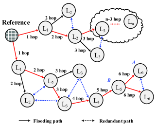
Figure 1: Network topology and flood model (diameter of $n$, e.g., $n\geq 6$), in which time information received from the reference is more accurate than that received from closer to the reference.

Therefore, both flooding path and time cost are important to flooding synchronization. In large-scale WSN applications, there are more than one paths between nodes and the flooding time costs are different on each path. Due to the clock shifting, the time information along the path that costs less time is more accurate [26, 27, 28]. Moreover, the clock drift is always changing, and as a result, the time information is becoming inaccurate, until it is forwarded, and it is likely that the longer the waiting time of time information forwarding, the worse the accuracy.

II-B Delay on One-Way Broadcast Model

A one-way broadcast model is used to collect timestamps in many time synchronization algorithms. The model broadcasts time packets at the real time $t$ to generate pairs of timestamps, e.g., $T_{s}$ (at the sender) and $T_{r}$ (at the receiver). If $D$ is the packet transmission delay and $\theta_{r}^{s}(t)$ is the relative clock offset, then $T_{r}-T_{s}=D+\theta_{r}^{s}(t)$. The relative clock offset estimation $\hat{\theta}_{r}^{s}(t)$ in one-way-broadcast-based time synchronization is

$$\hat{\theta}_{r}^{s}(t)=D+\theta_{r}^{s}(t).$$ (1)

In our previous experiments, we used the Start Frame Delimiter (SFD) interrupt to create MAC-layer timestamps and test $D$ when nodes ran in multi-tasking mode. Three interrupt sources were set for the testbed and three different priority levels configured for the test sequence, i.e., equal priority level for all of interrupt sources and lowest or highest priority level for SFD interrupt. Based on the experimental results (more than 500,000 observations were collected), we found that $D$ on one-way broadcast comprises two portions, i.e.,

$$D=D_{var}+D_{unc},$$ (2)

where $D_{var}$ is the variable delay and $D_{unc}$ is the uncertain delay. A summary of $D$ is shown in Table I.

TABLE I:
Summary of delay $D$ on one-way broadcast model. $D_{var}$, variable delay of $D$; $D_{unc}$, uncertain delay of $D$.

SFD	Variable delay $D_{var}$			Uncertain delay $D_{unc}$
interrupt priority	Probability	Mean (µs)	STD	Probability	Max. (µs)
Equal	0.8825	3.322	0.075	0.1175	910
Lowest	0.9463	3.330	0.075	0.0537	732
Highest	0.9987	3.312	0.072	0.0013	910

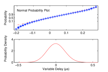
Figure 2: Probability and probability density of $d$. Parameter $d$ denotes the variable part of $D_{var}$. The Normal Probability Plot indicates that $d$ is gaussian, and $d\sim N(0,0.0049)$.

It is clear that $D_{var}$ is the main portion of $D$, and $D_{var}=D_{fixed}+d$, where $D_{fixed}$ is the fixed portion of $D_{var}$, and $d$ is the variable portion [30]. The maximum value of $D_{var}$ is approximately 3.6 µs and that of $\hat{D}_{fixed}$ (i.e., the mean of $D_{var}$) is 3.3 µs. After calculating the probability density of variable delay $d$, the results are shown in the bottom part of Fig. 2. The mean of $d$ is $0$ µs and the variance $\sigma^{2}$ is 0.0049. Using the t-test tool to test $d$, we obtained that $d$ is normal distribution with 99.99% confidence. The normal probability plot of $d$ is shown in the top part of Fig. 2 and indicates that all of the observations are close to the line and $d$ is Gaussian distributed, i.e., $d\sim N(0,\sigma^{2})$. Meanwhile, $D_{unc}$ has no statistical characteristics and is much larger than $D_{var}$, and it depends strictly on the implementation of timestamp, e.g., the software, interrupt nesting, and priority levels.

II-C Error Analysis

We define the synchronization error as $E$. Considering the multi-hop one-way broadcast flooding time synchronization (Synchronization interval of $T_{b}$), inevitable delay occurs when node floods the reference’s time information to its neighbors, which is defined as the flood waiting time $T_{wait}$ $(0<T_{wait}<T_{b})$. The clock offset estimation is calculated as in (1). Then the synchronization error on a single hop is $E[1]$, and

$$E[1]=D.$$ (3)

The relative clock frequency speed between $h$-hop and $(h-1)$-hop nodes is $a_{h}$. Then, the by-hop error accumulation on $k$ hops is

$$E[k]=\sum_{h=0}^{k-1}D[h]+\frac{\sum_{h=0}^{k-1}{(a[h]\times T_{wait}[h])}}{10^{6}},$$ (4)

where $D[h]$ is the delay on the $h$-hop ($D[h]=D_{fixed}+d[h]+D_{unc}[h]$), and $T_{wait}[h]$ is the corresponding forward latency.

The synchronization error of flooding time synchronization (FTSP) can be calculated by (4). It is clear that the synchronization error is determined by the delay $D$ and forward latency $T_{wait}$. The rapid-flooding protocols (e.g., Glossy, PulseSync and PulsePISync) minimize $T_{wait}$, and the FCSA and FloodPISync minimize $a[h]$. The FCSA employs the clock speed agreement to maintain $\hat{a}[h]$, and makes all of the nodes at the same speed. Then the synchronization error in FCSA and FloodPISync are given by

$$E_{F}[h]=\sum_{h=0}^{k-1}D[h]+\frac{\sum_{h=0}^{k-1}{((|a[h]-\hat{a}[h]|)\times T_{wait}[h])}}{10^{6}}.$$ (5)

The rapid-flooding algorithms minimize the forward latency, i.e., $T_{wait}[h]\rightarrow 0$. If the clock skew estimation is accurate enough, i.e., $\hat{a}[h]\rightarrow a[h]$, then the synchronization error in PulsePISync is

$$E_{PI}[h]\thickapprox\sum_{h=0}^{k-1}D[h].$$ (6)

Moreover, the PulseSync employs $\hat{D}_{fixed}$ to compensate for the delay $D$, then the synchronization error in PulseSync is

$$E_{P}[h]\thickapprox\sum_{h=0}^{k-1}(D[h]-\hat{D}_{fixed}).$$ (7)

However, the effect of variable $D_{unc}$ is much larger than that of $D_{var}$, and $D_{unc}$ is not considered in previous flooding time synchronization approaches. Specifically, $D_{var}$ is the main source of error for multi-hop time synchronization, which limits the time synchronization convergence accuracy. Meanwhile $D_{unc}$ may cause the entire network to be out of synchronization. According to (4), (5), (6), and (7), if a $D_{unc}$ is generated at the intermediate node of the flooding path, then all of the next hop nodes of this flooding path will be out of synchronization, and it will take a very long time to re-synchronize these nodes. According to (5) and (6), the PulsePISync is more accurate than FloodPISync, thus we will use PulsePISync to compare with RMTS.

III System Model

The WSN in this paper is modeled as the graph $G=(\mathcal{N},\mathcal{E})$, where $\mathcal{N}=\{1,2,\ldots\mathcal{N}\}$ represents the nodes of the WSN and $\mathcal{E}$ defines the available communication links. The set of neighbors for $v_{i}$ is $\mathcal{N}_{i}=\{j|(i,j)\in\mathcal{E},i\neq j\}$, where nodes $v_{i}$ and $v_{j}$ belong to $\mathcal{N}$, and $j\in\mathcal{N}_{i}$. There are two time notions defined for the time synchronization algorithm, i.e., the hardware clock $H(t)$ and logical clock $L(t)$.

The hardware clock $H(t)$ is defined as

$$H(t)=\int_{0}^{t}h(\tau)d\tau+\theta(t_{0}),$$ (8)

where $h(\tau)$ is the hardware clock rate, and it is the inherent attribute of the crystal oscillator and can never be changed or measured. Every node considers itself the ideal clock frequency (nominal frequency), i.e., $h(\tau)=1$. Constant $t_{0}$ is the moment that a node is powered on and $\theta(t_{0})$ is the initial relative clock offset. Therefore, $H(t)$ cannot be changed, and timestamps on $H(t)$ are used to estimate the relative clock speed for the proposed algorithm.

The logical clock $L(t)$ is defined as

$$L(t)=\varphi\times H(t),$$ (9)

where $\varphi$ is the logical clock rate multiplier and can be changed to speed up or slow down $L(t)$. The timestamps on $L(t)$ are created for clock offset estimation.

Considering the arbitrary nodes $v_{i}$ and $v_{j}$, $L_{i}(t)$ and $L_{j}(t)$ are the respective logical times, and $\varphi_{i}^{j}$ is the relative clock rate, which is

$$\varphi_{i}^{j}=1+\theta_{\Delta}/\tau,(\tau>0),$$ (10)

where $\theta_{\Delta}$ is the relative clock offset increment, and $\theta_{\Delta}=(H_{j}(t)-H_{i}(t))-(H_{j}(t-\tau)-H_{i}(t-\tau))$.

IV Proposed RMTS Algorithm

IV-A Proposed Multiple One-Way Broadcast

In multiple-one-way-broadcast model, nodes broadcast $N$ time information packets at very short time in a single synchronization period, and $N$ timestamps are generated at both sender and receivers. As shown in Fig. 3, $\{T_{k,x}[n]\}_{n=1}^{N}$ is set of timestamps on $v_{k}$ $(k\in G)$, where $x$ is the identity of the different synchronization process, and $n$ $(n\leq N)$ is the serial number of the one-way broadcast in the same synchronization process.

There are two important processes in the proposed multiple-one-way-broadcast model, i.e., $U$ and $V$, in which an observation set is collected for clock skew estimation and clock offset estimation, e.g., $\langle\{T_{r,1}[n]\}_{n=1}^{N},\{T_{j,1}[n]\}_{n=1}^{N}\rangle$ and $\langle\{T_{r,2}[n]\}_{n=1}^{N},\{T_{j,2}[n]\}_{n=1}^{N}\rangle$, respectively.

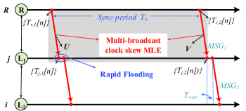
Figure 3: Multiple-one-way-broadcast model. Nodes broadcast $N$ times of information packets in a short time interval, then $n$ $(n\leq N)$ pairs of timestamps are generated for the RMTS, e.g., the $T_{r,1}[n]$ and $T_{j,1}[n]$ in process $U$.

IV-B Clock Skew Estimation

Here, we introduce MLE of relative clock skew $\hat{\varphi}_{j}^{r}$ for $v_{r}$ and $v_{j}$, which had been proposed in our previous work and proved to be more accurate than the Linear regression. Based on the down link $U$ and $V$ in Fig. 3, the clock skew estimation observations set $\{u[n],v[n]\}_{n=1}^{N}$ is calculated by

$$u[n]=T_{j,u}[n]-T_{r,u}[n]=D_{u}+\theta_{u}+d_{u}[n],$$ (11)

$$v[n]=T_{j,v}[n]-T_{r,v}[n]=D_{v}+\theta_{u}+\theta_{\Delta}+d_{v}[n],$$ (12)

where $D:\{D_{u},D_{v}\}$ are the fixed components of $D_{var}$ and $\{d_{u}[n],d_{v}[n]\}_{n=1}^{N}$ are the variable components of $D$. The parameter $\theta_{u}$ is the clock offset at $U$ and $\theta_{\Delta}$is the clock offset increment from $U$ to $V$. It is assumed that $D_{u}=D_{v}=D_{fixed}$ [30, 32] and $d$ can be modeled by Gaussian distribution. If $\hat{\theta}_{\Delta}=v[k]-u[k]$ and $\hat{\tau}=T_{j,v}[k]-T_{j,u}[k]$ $(k\in(0,N))$, then $\hat{\varphi}_{j}^{r}$, according to (10), is given by

$$\hat{\varphi}_{j}^{r}=\frac{\hat{\theta}_{\Delta}}{T_{j,v}[k]-T_{j,u}[k]}+1,$$ (13)

where $T_{j,v}[k]-T_{j,u}[k]\rightarrow T_{b}$. The estimation errors of $\hat{\varphi}_{j}^{r}$ completely depend on $\hat{\theta}_{\Delta}$, which is given as

$$\hat{\theta}_{\Delta}=\theta_{\Delta}+(d_{v}[k]-d_{u}[k]).$$ (14)

We define $P:\{p[k]=\theta_{\Delta}+(d_{v}[k]-d_{u}[k])\}_{k=1}^{N}.$ Since $d\sim N(\mu,\sigma^{2})$, then the probability distribution function of $\{d_{v}[k]-d_{u}[k]\}_{k=1}^{N}$ is given as

$$f(P)=\frac{1}{2\sqrt{\pi}\sigma}\exp(-\frac{p^{2}}{4\sigma^{2}}).$$ (15)

The likelihood function for $(\theta_{\Delta},\alpha,\sigma^{2})$ is given as

$$L(P;\theta_{\Delta},\alpha, \sigma^{2})$$ (16)

$$=\frac{1}{(2\sqrt{\pi}\sigma)^{N}}\exp(-\frac{\sum_{s=1}^{N}(p-\theta_{\Delta})^{2}}{4\sigma^{2}}).$$

Differentiating the log-likelihood function yields

$$\frac{\partial\ln L(P;\theta_{\Delta},\alpha,\sigma^{2})}{\partial\theta_{\Delta}}=\frac{1}{2\sigma^{2}}\sum_{s=1}^{N}(p-\theta_{\Delta}).$$ (17)

Therefore, the MLE of $\hat{\theta}_{\Delta}$ is given as

$$\hat{\theta}_{\Delta(MLE)} =\arg{\max{[\ln L(P;\theta_{\Delta},\alpha,\sigma^{2})]}}$$ (18)

$$=\frac{\sum_{s=1}^{N}p}{N}=\bar{P}.$$

The MLE of $\hat{\varphi}_{j}^{r}$ with the Gaussian delay model is given as

$$\hat{\varphi}_{j(MLE)}^{r}=\frac{\bar{P}}{\hat{\tau}},$$ (19)

where $\hat{\varphi}_{j(MLE)}^{r}$ is independent of clock offset estimation.

IV-C Clock Offset Estimation

Rewriting (1), the clock offset estimation error on a single hop is calculated as $D$. The MLE of clock offset estimation is simply calculated based on the multiple-one-way- broadcast model and the observations in (11) (i.e., $\{u[n]\}_{n=1}^{N}$), and is given by

$$\hat{\theta}_{i(MLE)}^{j}=\min_{1\leq n\leq N}{\{u[n]\}_{n=1}^{N}},$$ (20)

where the estimate error is $D_{fixed}+\min(\{d_{u}[n]\}_{n=1}^{N}),d\sim N(0,\sigma^{2})$. When using the statistical average of delays during a calibration phase [28, 29], i.e., $\hat{D}_{fixed}$ is rewritten as

$$\hat{\theta}_{i(MLE)}^{j}=\min_{1\leq n\leq N}{\{u[n]\}_{n=1}^{N}}-\hat{D}_{fixed}.$$ (21)

The clock offset estimate error is then $\min{(\{d-u[n]\}_{n=1}^{N})}$.

IV-D Proposed RMTS

A root (reference) algorithm and non-root algorithm are designed in the RMTS protocol.

1) Root algorithm

The root only broadcasts the time information packets and never handles the received time information packets. The pseudo-code of the root algorithm is presented in Algorithm 1. The $\varphi_{R}$ of the root is a constant value and can never be changed, i.e., $\varphi_{R}=1$ (Algorithm 1, Line IV-D). If there is an external clock $L_{ExtRef}$ for the root, such as GPS, the root can synchronize its logical time $L_{R}$ to $L_{ExtRef}$ (Algorithm 1, Lines IV-D and IV-D). Then, the logical time of the root is updated by $L_{R}(t+\tau)=(H_{R}(t+\tau)-H_{R}(t))+L_{ExtRef}(t),\tau\geq 0$; else, $L_{R}(t)=H_{R}(t)$.

The root broadcasts periodically to distribute the reference time information packets to neighbors, as in Algorithm 1, Lines LABEL:alg1.6-LABEL:alg1.11. Once the broadcast task is triggered, the root rapidly broadcasts $N$ packets in a very short time interval (there is a fixed clock offset for each broadcast), as in Algorithm 1, Lines LABEL:alg1.7-LABEL:alg1.9. Two groups of timestamps are created over the phase of broadcasting, i.e., timestamp $H_{R}[n]$ (created on $H_{R}(t)$) and timestamp $L_{R}[n]$ (created on $L_{R}(t)$). The basic information of the broadcast packets comprises four parts: $H_{R}[n]$, $L_{R}[n]$, $\varphi_{R}$, and $ID_{R}$ (Algorithm 1, Line LABEL:alg1.8).

2) Non-root algorithm

The pseudo-code of the non-root algorithm is presented in Algorithm 2. Node $v_{i}$ is synchronized to the root by calibrating $L_{i}(t)$ based on the rate multiplier $\varphi_{i}$ and clock offset estimation $\hat{\theta}_{i(MLE)}^{j}$, where $v_{j}$ is the neighbor of $v_{i}$ and is closer to the root.

1 Initialization:

2  Set $\varphi_{R}=1$, $ID_{R}=1$, $n=0$

3  Start periodic broadcast task, period of $T_{b}$

4 if external clock is used then

5       Set $L_{R}(t)\leftarrow L_{ExtRef}(t)$

6      

7 end if

Algorithm 1 Root algorithm pseudo-code for RMTS. $v_{R}$ is the root node and $N$ is the maximal number of multiple broadcasts.