Excitation Spectra of one-dimensional spin-1/2 Fermi gas with an attraction

Abstract

Using exact Bethe ansatz solution, we rigorously study excitation spectra of the spin-1/2 Fermi gas (called Yang-Gaudin model) with an attractive interaction. Elementary excitations of this model involve particle-hole excitation, hole excitation and adding particles in the Fermi seas of pairs and unpaired fermions. The gapped magnon excitations in spin sector show a ferromagnetic coupling to the Fermi sea of the single fermions. By numerically and analytically solving the Bethe ansatz equations and the thermodynamic Bethe ansatz equations of this model, we obtain excitation energies for various polarizations in the phase of the Fulde-Ferrell-Larkin-Ovchinnikov (FFLO)-like state. For a small momentum (long-wavelength limit) and in the strong interaction regime, we analytically obtained their linear dispersions with curvature corrections, effective masses as well as velocities in particle-hole excitations of pairs and unpaired fermions. Such a type of particle-hole excitations display a novel separation of collective motions of bosonic modes within paired and unpaired fermions. Finally, we also discuss magnon excitations in spin sector and the application of the Bragg spectroscopy for testing such separated charge excitation modes of pairs and single fermions.

Keywords: Yang-Gaudin Model, quantum integrability, the Bethe ansatz, excitation spectrum

I Introduction

The quantum many-body systems manifest abundant physical phenomena, such as Bose-Einstein Condensation (BEC), superfluidity, superconductivity, and quantum phase transition, etc., which are regarded as the emergent phenomena in modern physics. However, the complexity of many-body systems, involving a huge internal degrees of freedom, quantum statistics and interaction, alway brings us a formidable task to access their physics of interest. Among the known many-body theories, there are two universal low energy effective theories, i.e. Fermi liquid and Tomonaga-Luttinger liquid that capture significant different features of many-body correlations in one dimension (1D) and higher dimensions. Landau Fermi Liquid theory baym2008landau ; landau1957oscillations ; landau1956fermi remarkably describes metallic behaviour of interacting fermions in 2D and 3D. In this theory the concept of quasiparticles reveals the essence of individual particle excitations close to the Fermi surface in the interacting fermions. In contrast, when the degrees of freedom are reduced to 1D, the elementary excitations in 1D systems strikingly form collective motions of bosons, which are named the Tomonaga-Luttinger liquid (TLL) in the long-wavelength limit tomonaga1950remarks ; luttinger1963exactly . In the TLL theory, the low energy behaviour of 1D systems can be universally described by the bosonic fields of quantized sound waves or phonons. Early theoretical frame work of the TLL for various 1D problems was developed by Lieb and Mattismattis1994exact , Haldane haldane1981luttinger and others, see reviews giamarchi2003quantum ; Cazalilla2011one . The TLL has become the main theme in the study of critical behaviour of 1D many-body systems.

On the other hand, integrable models provide significant insight into the emergent phenomena driven by interactions and quantum statistics in low and higher dimensions essler2005one ; Cazalilla2011one ; guan2013fermi . The quantum integrability should trace back to H. Bethe’s work in 1931 when he solved the eigenvalue problem of 1D spin-1/2 Heisenberg chain bethe1931theorie by writing the wave function of the model as the superposition of all possible plane waves. It was over 30 years after Bethe’s work that this method was coined as the BA (Bethe ansatz) by C. N. Yang and C. P. Yang in their series of publications in mid-60’s YY-1 ; YY-2 ; YY-3 . Using Bethe’s method, Lieb and Liniger lieb1963exact solved the 1D Bose gas with a $\delta$-function interaction, which is now called the Lieb-Liniger model. In 1964 J. Mcguiremcguire1964study studied the 1D Fermi gas with the $\delta$-function interaction by considering the exact solution of one spin-up fermion interacting with $N-1$ spin-down fermions. The exact solution of the 1D Fermi gas with arbitrary numbers of spin-up and spin-down particles was solved by Yang yang1967some ; yang1968s , while at that time M. Gaudin gaudin1967systeme obtained the BA solution for the model with a spin balance. This model is now named the Yang-Gaudin model. In C. N. Yang’s seminal work yang1967some , a key discovery of the necessary condition for the BA solvability was surprisingly found. In 1972, R. J. Baxter baxter1972partition independently showed that such a factorization relation also occurred as the conditions for commuting transfer matrices in 2D vertex models in statistical mechanics. It is now known as the Yang-Baxter equation, i.e. the factorization condition. The Yang-Baxter equation has laid out a profound legacy in a variety of fields in mathematics and physics.

In 1969, C. N. Yang and C. P. Yang yang1969thermodynamics obtained the thermodynamics of the Lieb-Liniger Bose gas at finite temperatures. They found that the thermodynamics of the model can be determined by the minimisation conditions of the Gibbs free energy in terms of the microscopic states determined by the BA equations. M. Takahashi generalized Yang and Yang’s method to deal with the thermodynamics of the 1D Heisenberg spin chain and 1D Hubbard model though introducing string hypotheses takahashi2005thermodynamics ; takahashi1970ground ; takahashi1970many ; takahashi1994one ; takahashi1970magnetic . He coined the method as the Yang-Yang thermodynamic Bethe ansatz (TBA), see a feature review guan2019professor . Further developments of the TBA approach have been made in the study of universal thermodynamics, Luttinger liquid, spin-charge separation, transport properties and critical phenomena for a wide range of low-dimensional quantum many-body systems, see reviews guan2013fermi ; Guan:2022 .

In the attractive regime, the Yang-Gaudin model exhibits novel Fulde-Ferrell-Larkin-Ovchinnikov (FFLO) pairing correlation ff1964 ; lo1965 , i.e. coexistence of paired and unpaired fermions 70-75in-Guan-Lin'spaper . Understanding of the FFLO pairing behavior in 1D and higher dimensions is still an open challenge in condensed matter physics. The phase diagram of the attractive Fermi gas, consisting of a fully-paired state for an external field is less than the lower critical field $H_{c1}$, a fully-polarized state for the magnetic field is greater than an upper critical field $H_{c2}$ and the FFLO-like state lies in between the two critical fields, was predicted in guan2007phase ; orso2007attractive ; hu2007phase and experimentally confirmed by R. Hulet’s group in liao2010spin . This novel phase diagram reveals striking features of thermodynamics, for instance, universal behaviour of the specific heat guan2011quantum , the dimensionless ratios, such as Grüneisen parameter peng2019gruneisen and Wilson ratios guan2013wilson ; yu2016dimensionless . The dark-soliton-like excitations in the Yang-Gaudin gas of attractively interacting fermions and the Lieb-Liniger gas shamailov2016dark ; shamailov2019quantum shed light on the nonlinear effects of many-body correlation. Nevertheless, one expects that the elementary excitations in this attractive Yang-Gaudin model would provide significant collective nature of multi-component TLLs with pairing and depairing in thermodynamics and dynamic response functions. This is the major research of the following study in this paper.

In Section II, we will introduce the BA equations and TBA equations, which will be used to accomplish our study of the excitation spectra of the Yang-Gaudin model with an attraction. In Section III, we will present the particle-hole excitation spectra in paired and unpaired fermi seas. In Section IV, we will analytically derive dispersion relations with band curvature corrections, effective mass and sound velocities of pairs and unpaired fermions for the Yang-Gaudin model with polarizations in a strong coupling regime. In section V, we will discuss multiple particle-hole excitations and the magnon excitations in the FFLO-like phase. The last Section is remained for our conclusion and discussion.

II Yang-Gaudin Model with an Attractive Interaction

II.1 Bethe Ansatz Equations and String Hypotheses

The 1D two-component Fermi gas with a delta-function interaction is called the Yang-Gaudin modelyang1967some ; yang1968s ; gaudin1967systeme . Its Hamiltonian is given by

$$\mathcal{H}=-\sum_{i=1}^{N}\frac{\partial^{2}}{\partial x_{i}{}^{2}}+4c\sum_{i<j}\delta\left(x_{i}-x_{j}\right)-\mu_{0}H\left(N-2N_{\downarrow}\right),$$ (1)

where $N$ is the number of fermions, $N_{\downarrow}$ is the number of down-spin fermions, $H$ is the external magnetic field, $c<0$ for attractive interaction, and herewith we set $\hbar^{2}=2m=1$. We always choose an upward magnetic field so that spin-down fermions are less than spin-up ones. As a result, each spin-down fermion can be paired with a spin-up fermion and form a bounded state. While the remaining spin-up fermions are unpaired and in polarized state. Denote the number of paired fermions as $M$, then that of unpaired fermions is $N-2M$.

The quasimomenta $\{k_{j}\}$ of the fermions and the rapidities $\{\Lambda_{\alpha}\}$ of the spin-down fermions are given by the BA Equations

$$e^{ik_{j}L}=\prod_{\alpha=1}^{N_{\downarrow}}e\left(\frac{k_{j}-\Lambda_{\downarrow\alpha}}{c}\right),$$ (2)

$$\prod_{j=1}^{N}e\left(\frac{\Lambda_{\downarrow\alpha}-k_{j}}{c}\right)=\prod_{\beta\neq\alpha}e\left(\frac{\Lambda_{\downarrow\alpha}-\Lambda_{\downarrow\beta}}{2c}\right)$$

for $j=1,2,\cdots,N$ and $\alpha=1,2,\cdots,N_{\downarrow}$, where $e\left(x\right)=\exp\left(i\pi-2i\arctan{x}\right)$.

Takahashitakahashi2005thermodynamics ; takahashi1970ground ; takahashi1970many ; takahashi1994one ; takahashi1970magnetic introduced the following spin string hypotheses for the root patterns of the BA equations (2):
1. Complex $\Lambda_{\downarrow\alpha}$ always forms a bound state with several other $\Lambda_{\downarrow\alpha}$’s. In this set of $n$-$\Lambda_{\downarrow\alpha}$’s the real parts are the same and the imaginary parts are $(n-1)ci,(n-3)ci,\cdots,-(n-1)ci$ for each of them within the accuracy of $\mathcal{O}(\exp(-\delta N))$, where $\delta$ is a positive number. This bound state of $n$-$\Lambda_{\downarrow\alpha}$’s forms an $n$-string. In the following discussion, we will denote each of these complex $n$-$\Lambda_{\downarrow\alpha}$ strings as $\Lambda_{\alpha}{}^{n,j}$, where $j=1,2,,\cdots,n$. We suppose that there are $M_{n}$-$n$-strings, and denote their real part of each $n$-string as $\Lambda_{\alpha}{}^{n}$, where $\alpha=1,2,\cdots,M_{n}$. Than we can express the $n$-string as

$$\Lambda_{\alpha}^{n,j}=\Lambda_{\alpha}{}^{n}+(n+1-2j)ci+\mathcal{O}(\exp(-\delta N)),j=1,2,\cdots,n.$$ (3)

2. For an attractive interaction $c<0$, a pair of quasi-momenta form a charge bound sate, namely $k_{\alpha}$ and its complex conjugate $\bar{k}_{\alpha}$ have a common real part $\Lambda$, i.e.,

$$k_{\alpha}=\Lambda_{\alpha}+i\left|c\right|+\mathcal{O}\left(\exp\left(-\delta L\right)\right),$$ (4)

$$\bar{k}_{\alpha}=\Lambda_{\alpha}-i\left|c\right|+\mathcal{O}\left(\exp\left(-\delta L\right)\right).$$

Supposing that there are $M$ charge bound pairs and $\left(N-2M\right)$ single fermions with the quasi-momenta $\left\{k_{j}\right\}$ with $j=1,2,\cdots,N-2M$. Then the BA equations (2) can be rewritten in the following form takahashi1994one

$$2\Lambda_{\alpha}L=2\pi J_{\alpha}+\sum_{j=1}^{N-2M}\theta\left(\frac{\Lambda_{\alpha}-k_{j}}{|c|}\right)+\sum_{\beta=1}^{M}\theta\left(\frac{\Lambda_{\alpha}-\Lambda_{\beta}}{2|c|}\right),\quad\alpha=1,2,\cdots,M$$ (5)

$$k_{j}L=2\pi I_{j}+\sum_{\alpha=1}^{M}\theta\left(\frac{k_{j}-\Lambda_{\alpha}}{|c|}\right)+\sum_{n=1}^{\infty}\sum_{\alpha=1}^{M_{n}}\theta\left(\frac{k_{j}-\Lambda_{\alpha}{}^{n}}{n|c|}\right),\quad j=1,\cdots,N-2M$$

$$\sum_{j=1}^{N-2M}\theta\left(\frac{\Lambda_{\alpha}{}^{n}-k_{j}}{n|c|}\right)=2\pi J_{\alpha}{}^{n}+\sum_{m=1}^{\infty}\sum_{\beta=1}^{M_{m}}\Theta_{nm}\left(\frac{\Lambda_{\alpha}{}^{n}-\Lambda_{\beta}^{m}}{|c|}\right),\quad\begin{array}[]{l}\alpha=1,2,\cdots,M_{n}\\ n=1,2,\cdots.\end{array}$$

where $\theta\left(x\right)=2\arctan x,-\pi<\theta<\pi$, and

$$\Theta_{nm}\left(x\right)$$ (6)

$$= \begin{cases}\theta\left(\frac{x}{|n-m|}\right)+2\theta\left(\frac{x}{|n-m|+2}\right)+2\theta\left(\frac{x}{|n-m|+4}\right)+\cdots+2\theta\left(\frac{x}{n+m-2}\right)+\theta\left(\frac{x}{n+m}\right)&\text{ for }n\neq m\\ 2\theta\left(\frac{x}{2}\right)+2\theta\left(\frac{x}{4}\right)+\cdots+2\theta\left(\frac{x}{2n-2}\right)+\theta\left(\frac{x}{2n}\right)&\text{ for }n=m\end{cases}.$$

Here $J_{\alpha}$ is integer (half-odd integer) for $N-M$ odd (even), $I_{j}$ is integer (half-odd integer) for $M+M_{1}+M_{2}+\cdots$ even (odd), and $J_{\alpha}{}^{n}$ is integer (half-odd integer) for $N-M_{n}$ odd (even). $J_{\alpha}{}^{n}$ should satisfy the condition

$$\left|J_{\alpha}{}^{n}\right|\leqq\frac{1}{2}\left(N-2M-\sum_{m=1}^{\infty}t_{nm}M_{m}\right),\quad t_{mn}=2\mathrm{min}\left(n,m\right)-\delta_{n,m}.$$ (7)

Eq.(5) give quantum numbers $J_{\alpha}$, $I_{j}$, and $J_{\alpha}{}^{n}$ for charge sector of paired fermions, charge sector of unpaired fermions, and spin sector of unpaired fermions, respectively. It turns out that for each pair $k_{\alpha}$ and $\bar{k}_{\alpha}$ are given by $\Lambda_{\alpha}$, representing quasi-momenta of pairs. Whereas $k_{j}$ represent quasi-momenta of $N-2M$ unpaired fermions and $\Lambda_{\alpha}{}^{n}$ represent $M_{n}$ spin wave bound states (the length-$n$ strings).

In the thermodynamic limit, i.e., $L,\,N\rightarrow\infty$, these quantum numbers could be treated as functions of continuous variables $k$s, which satisfy

$$\mathrm{d}J_{\alpha}\left(k\right)=L\left(\sigma\left(k\right)+\sigma^{h}\left(k\right)\right)\mathrm{d}k,$$ (8)

$$\mathrm{d}I_{j}\left(k\right)=L\left(\rho\left(k\right)+\rho^{h}\left(k\right)\right)\mathrm{d}k,$$

$$\mathrm{d}J_{\alpha}{}^{n}\left(k\right)=L\left(\sigma_{n}\left(k\right)+\sigma_{n}^{h}\left(k\right)\right)\mathrm{d}k,$$

where $\sigma,\rho,\sigma_{n}$ denote distribution functions of bound pairs, single particles and length-$n$ spin strings, respectively. While $\sigma^{h},\rho^{h},\sigma_{n}^{h}$ denote the distribution functions of their corresponding holes. The continuous $k$ stands for discrete quasi-momenta $k_{j}$, $\Lambda_{\alpha}$ and $\Lambda_{\alpha}{}^{n}$. It follows that the BA equations (2) become as takahashi1994one

$$\frac{1}{\pi}=\sigma+\sigma^{n}+[2]\sigma+[1]\rho$$ (9)

$$\frac{1}{2\pi}=\rho+\rho^{h}+[1]\sigma+\sum_{n}[n]\sigma_{n}$$

$${[n]\rho=\sigma_{n}{}^{h}+\sum_{m}A_{nm}\sigma_{m}},$$

where $[n]$ is an operator defined by

$$[n]f\left(k\right)=\int_{-\infty}^{\infty}a_{n}\left(k-k^{\prime}\right)f\left(k^{\prime}\right)dk^{\prime},\quad a_{n}\left(k\right)=\frac{1}{\pi}\frac{n|c|}{\left(nc\right)^{2}+k^{2}},$$ (10)

$$[0]f\left(k\right)=f\left(k\right).$$

Here

$$A_{nm}=[|n-m|]+2[|n-m|+2]+2[|n-m|+4]+\cdots+2[n+m-2]+[n+m].$$ (11)

II.2 Thermodynamical Bethe Ansatz Equations and Thermodynamic Quantities

Building on microscopic state energies, we may further define dressed energies of pairs $\varepsilon=T\ln{\eta}$, single fermions $\kappa=T\ln{\zeta}$, and length-$n$ strings $\varepsilon_{n}=T\ln{\zeta_{n}}$, respectively. Here we denoted the quantities $\zeta=\rho^{h}/\rho,$ $\eta^{=}\sigma^{h}/\sigma,$ and $\eta_{n}=\sigma_{n}^{h}/\sigma_{n}$. Minimizing thermodynamic potential $\Omega\equiv E-TS-AN-HS_{Z}$ with respect to the densities though Eq.(9), i.e., $\delta\Omega=0$, we may obtain the following blueTBA Equations takahashi1994one

$$\ln\eta^{=}\frac{2\left(k^{2}-A-c^{2}\right)}{T}+[2]\ln\left(1+\eta^{-1}\right)+[1]\ln\left(1+\zeta^{-1}\right),$$ (12)

$$\ln\zeta=\frac{k^{2}-A-\mu_{0}H}{T}+[1]\ln\left(1+\eta^{-1}\right)-\sum_{n=1}^{\infty}[n]\ln\left(1+\eta_{n}^{-1}\right),$$

$$\ln\left(1+\eta_{n}\right)=\frac{2n\mu_{0}H}{T}+[n]\ln\left(1+\zeta^{-1}\right)+\sum_{m=1}^{\infty}A_{nm}\ln\left(1+\eta_{m}^{-1}\right),$$

where $n=1,\dots,\infty$. In the above equations, $T$, $A$ and $H$ stand for temperature, chemical potential and magnetic field, respectively. Accordingly, we can give the equation of state, namely the pressure $p$ is given by

$$p=-\Omega/L=T\int_{-\infty}^{\infty}\ln\left(1+\eta^{-1}\right)\frac{\mathrm{d}k}{\pi}+T\int_{-\infty}^{\infty}\ln\left(1+\zeta^{-1}\right)\frac{\mathrm{d}k}{2\pi},$$ (13)

The pressure of this system is simply the sum of two terms, the term regarding the paired Fermi sea and another regarding the unpaired sea, respectively. Other thermodynamic quantities can be calculated through the usual thermodynamics relations:

$$N/L=\frac{\partial p}{\partial\mu},\quad S_{z}/L=\frac{\partial p}{\partial H},\quad S/L=\frac{\partial p}{\partial T},\quad\kappa=\frac{\partial^{2}p}{\partial A^{2}},\quad\chi=\frac{\partial^{2}p}{\partial H^{2}},\quad c_{V}=T\frac{\partial^{2}p}{\partial T^{2}},$$ (14)

where the last three quantities are the compressibility, magnetic susceptibility, and specific heat.

At the zero temperature $T\rightarrow 0$, due to the ferromagnetic ordering, we observe that $\eta_{n}\rightarrow\infty$ and $\sigma_{n}=0$ for $n=1,2,\cdots$ and the TBA equations (12) reduce to

$$\varepsilon\left(k\right)=2\left(k^{2}-A-c^{2}\right)-[2]\varepsilon^{-}\left(k\right)-[1]\kappa^{-}\left(k\right),$$ (15)

$$\kappa\left(k\right)=k^{2}-A-\mu_{0}H-[1]\varepsilon^{-}\left(k\right),$$

where the superscript ’$-$’ means the corresponding quantities are token the negative parts. Since $\varepsilon_{n}{}^{-}\rightarrow 0$ for $n\geq 1$ in the limit $T\rightarrow 0$, these equations are referred to the zero temperature dressed energy equations. In this case, the Fermi points $B$, $Q$ are determined by $\varepsilon\left(B\right)=0$ and $\kappa\left(Q\right)=0$. It turns out that $\varepsilon\left(k\right)$ and $\kappa\left(k\right)$ are monotonically increasing functions of $k^{2}$. Therefore, $B$ and $Q$ are Fermi surfaces referring to the continuous quasimomentum of paired and unpaired fermions. They can also be determined by the relations

$$n \equiv: \frac{N}{L}=2\int_{-B}^{B}\sigma(k)dk+\int^{Q}_{-Q}\rho(k)dk,$$

$$n_{\downarrow} \equiv: \frac{N_{\downarrow}}{L}=\int_{-B}^{B}\sigma(k)dk.$$ (16)

Thus the distribution functions are given by

$$\sigma\left(k\right)+\sigma^{h}\left(k\right)=\frac{1}{\pi}-\int_{-B}^{B}a_{2}\left(k-k^{\prime}\right)\sigma\left(k^{\prime}\right)\mathrm{d}k^{\prime}-\int_{-Q}^{Q}a_{1}\left(k-k^{\prime}\right)\rho\left(k^{\prime}\right)\mathrm{d}k^{\prime},$$ (17)

$$\rho\left(k\right)+\rho^{h}\left(k\right)=\frac{1}{2\pi}-\int_{-B}^{B}a_{1}\left(k-k^{\prime}\right)\sigma\left(k^{\prime}\right)\mathrm{d}k^{\prime},$$

where $\sigma_{n}=0$ for the ground state and spin sector is completely gapped.

Moreover, at zero temperature limit $T\rightarrow 0$, there exists the phase transition among fully paired phase, fully-polarized phase, partially-polarized phase, and vacuum phase, which will be further studied in Section IV.1. The fully paired phase can be regarded as the Bardeen-Cooper-Schrieffer(BCS) like phase, which is expected to manifest the first-type superconductivity. The phase diagram are given in orso2007attractive ; hu2007phase ; guan2011quantum ; yin2011quantum . Fulde and Ferrellff1964 and Larkin and Ovchinnikovlo1965 predicted the exotic superfluid phase, which is now called the FFLO phase. The partially polarized phase in the attractive Yang-Gaudin model is composed of BCS-like pairs and unpaired fermions, presenting a 1D-analogy of the FFLO phase. The FFLO-like phase diagram of the attractive Fermi gas was experimentally confirmed by Hulet’s group pini2021strong .

III Spectra of One-particle-hole Excitations

III.1 Ground State

Consider the partially polarized phase, where paired and unpaired fermions coexist. The total momentum of the system is given by

$$K=2\sum_{\alpha=1}^{M}\Lambda_{\alpha}+\sum_{j=1}^{N-2M}k_{j}=\frac{2\pi}{L}\left(\sum_{\alpha=1}^{M}J_{\alpha}+\sum_{j=1}^{N-2M}I_{j}+\sum_{n=1}^{\infty}\sum_{\alpha=1}^{M_{n}}J_{\alpha}{}^{n}\right)=K_{b}+K_{u}+K_{s,u}.$$ (18)

Due to the ferromagnetic ordering in spin sector, the distribution functions $\sigma_{n}=0$ with $n=1,2,\cdots$ at the ground state. In other words, there is no particle for the length $n$-strings, i.e., $M_{n}$=0. Therefore, the spin sector of unpaired fermions does not have contribution to the total momentum, i.e., $K_{s,u}=0$ at the ground state.

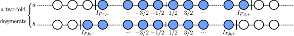
Figure 1: Schematic illustration of the two-fold degeneration. $I_{F,a,-}$ and $I_{F,a,+}$, (or $I_{F,b,-}^{\prime}$ and $I_{F,b,+}^{\prime}$ ) give respectively the Fermi points of unpaired (paired) sector. In this case, the particle number is odd while the corresponding quantum number $I_{j}$s take half-odd integers. It appears that these quantum numbers cannot distribute symmetrically. Therefore, the total momentum is non-zero and the ground state is two-fold degenerate.

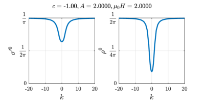
(a) density distributions

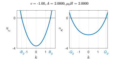
(b) dressed energies

Figure 2: (a) Density distribution functions and (b) Dressed energies at zero temperature. (a) For $k\rightarrow\pm\infty$, the density distributions of paired fermions $\sigma^{0}$ and unpaired fermions $\rho^{0}$ tend to $1/\pi$ or $1/(2\pi)$, respectively. (b) The dressed energies of paired and unpaired fermions are monotonically increasing with $|k|$. Therefore, the Fermi points referring to the continuous quasi-momenta can be well defined by the conditions $\varepsilon^{0}(\pm B_{0})=0$ and $\kappa^{0}(\pm Q_{0})=0$, respectively.

For the ground state, both paired and unpaired fermions should occupy those lowest-energy states, i.e., states with the lowest absolute quantum numbers (quasi-momenta). Consequently, most contributions of particles to total momentum are neutralized in the sum of positive and negative quantum numbers. The total momentum is not zero only if the distribution of quasi-momenta is not symmetric around the zero quasi-momentum. Fig.1 presents an example of non-zero total momentum, which essentially shows a two-fold degeneration.

There are totally $M$ paired fermions, whereas $J_{\alpha}$s take integers (half-odd integers) for $N-M$ odd (even). Therefore, $J_{\alpha}$s are symmetrically distributed if and only if $N$ is even. Similarly, there are $N-2M$ unpaired fermions, whereas $I_{j}$s take integers (half-odd integers) for $M+\sum M_{n}=M$ are even (odd). Therefore, $I_{j}$ is symmetrically distributed if and only if $N+M$ is odd, see Eq.(5). Consequently,

$$K_{b}=\begin{cases}0&\text{for }N\text{ even},\\ \pm\pi n_{b}&\text{for $N$ odd},\end{cases}\qquad K_{u}=\begin{cases}0&\text{for $N+M$ odd},\\ \pm\pi n_{u}&\text{for $N+M$ even},\end{cases}$$ (19)

where $n_{b}=M/L$ and $n_{u}=(N-2M)/L$ are particle densities of paired and unpaired sectors, respectively.

Introduce the superscript "$0$" to denote the ground state. Accordingly, the dressed-energies Eq.(15) and the density distribution functions and Eq.(17) are respectively written as

$$\sigma^{0}\left(k\right) =\frac{1}{\pi}-\int_{-B_{0}}^{B_{0}}a_{2}\left(k-k^{\prime}\right)\sigma^{0}\left(k^{\prime}\right)\mathrm{d}k^{\prime}-\int_{-Q_{0}}^{Q_{0}}a_{1}\left(k-k^{\prime}\right)\rho^{0}\left(k^{\prime}\right)\mathrm{d}k^{\prime}$$ (20)

$$\rho^{0}\left(k\right) =\frac{1}{2\pi}-\int_{-B_{0}}^{B_{0}}a_{1}\left(k-k^{\prime}\right)\sigma^{0}\left(k^{\prime}\right)\mathrm{d}k^{\prime}$$

and

$$\varepsilon^{0}\left(k\right) =2\left(k^{2}-A-c^{2}\right)-\int_{-B_{0}}^{B_{0}}a_{2}\left(k-k^{\prime}\right)\varepsilon^{0}\left(k^{\prime}\right)\mathrm{d}k^{\prime}-\int_{-Q_{0}}^{Q_{0}}a_{1}\left(k-k^{\prime}\right)\kappa^{0}\left(k^{\prime}\right)\mathrm{d}k^{\prime}$$ (21)

$$\kappa^{0}\left(k\right) =k^{2}-A-\mu_{0}H-\int_{-B_{0}}^{B_{0}}a_{1}\left(k-k^{\prime}\right)\varepsilon^{0}\left(k^{\prime}\right)\mathrm{d}k^{\prime},$$

both of which are plotted in Fig. 2 with certain values of the interaction strength, chemical potential and magnetic field, i.e. $\{c,A,\mu_{0}H\}$.

In terms of the additivity of the total momentum in Eq.(18), we can naturally define the Fermi points, $k_{F,b,\pm}$ and $k_{F,u,\pm}$, referring to the discrete quasimomenta of both paired and unpaired sectors, by maximal and minimal quantum numbers within occupied $\{J_{\alpha}\}$ and $\{I_{j}\}$, respectively. For $J_{\alpha}$ symmetrically distributed, $\left|k_{F,b,\pm}\right|=2\pi\left|J_{F,\pm}\right|/L=\pi(M-1)/L\approx\pi n_{b}$ for a thermodynamical limit, i.e. $N$, $L\rightarrow\infty$; whereas for the asymmetrical case, we still have $\left|k_{F,b,+}\right|=\pi(M-1\pm 1)/L\approx\pi n_{b}$ and $\left|k_{F,b,-}\right|=\pi(M-1\mp 1)/L\approx\pi n_{b}$, where the additional terms $\pm\pi/L$ emerging due to the two-fold degeneration are negligible for the thermodynamical limit. With similar regard, we have $k_{F,u,\pm}=2\pi I_{F,\pm}\approx\pi n_{u}$ for the Fermi points referring to the unpaired fermions. The Fermi points are referred to the conditions $\varepsilon^{0}\left(Q_{0}\right)=0$ and $\sigma^{0}\left(B_{0}\right)=0$, where $B_{0}$ and $Q_{0}$ are different from the quasimomenta $k_{F,b,\pm}$ and $k_{F,u,\pm}$ of pairs and unpaired fermions.

III.2 Sound Velocity and Effective Mass for One-Particle-hole Excitation

Figure 3: Schematic illustration of the one-particle-hole excitation: Moving one particle within the two Fermi points to outside the Fermi sea.

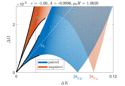
Figure 4: One-particle-hole excitation spectra of paired (blue) and unpaired (dark brown) fermions. $k_{F,b}$ ($v_{b}$) and $k_{F,u}$ ($v_{u}$) are the Fermi momenta (velocities) of paired and unpaired fermions, respectively. For small $\Delta K$, the paired and unpaired excitation spectra tend to the linear dispersions with different velocities $v_{b}$ and $v_{u}$, which are indicated by the white and green dashed lines, respectively. The curvature effects of these dispersion can be conceived from the effective masses which were further studied in Section IV. In this figure, we set $c=-1.00$, $A=-0.9996$, $\mu_{0}H=1.0020$ for our numerical calculation with the dispersions represented by Eqs.(24), (25) and (26).

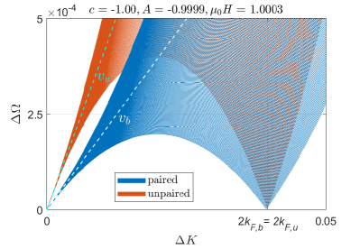
(a) $k_{F,b}=k_{F,u}$

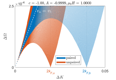
(b) $v_{u}=v_{b}$

Figure 5: One-particle-hole excitation spectra of paired (blue) and unpaired (dark brown) fermions with $k_{F,b}=k_{F,u}$ (a) and $v_{u}=2v_{b}$ (b). In (a), we set $c=-1.00$, $A=-0.9999$, $\mu_{0}H=1.0003$ for our numerical calculation with the Eqs.(24), (25) and (26); In (b), we set $c=-1.00$, $A=-0.9999$, $\mu_{0}H=1.0003$. These parameters are artificially selected, which we will explain in Section IV.

Consider one particle-hole excitation of unpaired fermions, where one quasiparticle with a quasimomentum $k_{h}$ inside the Fermi points is excited outside the Fermi points with a quasimomentum $k_{p}$, i.e.,

$$\rho\left(k\right)\neq 0,\text{ only for }k\in\left[Q_{-},k_{h}\right)\cup\left(k_{h},Q_{+}\right]\text{ and }k=k_{p}.$$

Define $\bar{\rho}\left(k\right)=\rho\left(k\right)+\rho^{h}\left(k\right)$, which is changed by $\Delta\bar{\rho}\left(k\right)$ after the excitation. Since there is exactly one excited hole inside the Fermi points and one quasiparticle outside,

$$\int_{-Q}^{Q}\Delta\bar{\rho}\left(k\right)L\mathrm{d}k=-1,\quad\left(\int_{-\infty}^{-Q}+\int_{Q}^{\infty}\right)\Delta\bar{\rho}\left(k\right)L\mathrm{d}k=1.$$

Therefore, $\Delta\bar{\rho}\left(k\right)$ is the sum of two $\delta$-functions, $-\delta(k-k_{h})/L$ and $\delta(k-k_{p})/L$. Also define $\bar{\sigma}\left(k\right)=\sigma\left(k\right)+\sigma^{h}\left(k\right)$. Consequently, the distribution functions Eq.(17) are rewritten as

$$\bar{\sigma}\left(\lambda\right)= \frac{1}{\pi}-\int_{B_{-}}^{B_{+}}a_{2}\left(\lambda-k^{\prime}\right)\sigma\left(k^{\prime}\right)\mathrm{d}k^{\prime}-\int_{Q_{-}}^{Q_{+}}a_{1}\left(\lambda-k^{\prime}\right)\bar{\rho}\left(k^{\prime}\right)\mathrm{d}k^{\prime}+\frac{1}{L}a_{1}\left(\lambda-k_{h}\right)-\frac{1}{L}a_{1}\left(\lambda-k_{p}\right)$$ (22)

$$\bar{\rho}\left(k\right)= \frac{1}{2\pi}-\int_{B_{-}}^{B_{+}}a_{1}\left(k-k^{\prime}\right)\sigma\left(k^{\prime}\right)\mathrm{d}k^{\prime},$$

where $B_{\pm}$ and $Q_{\pm}$ are fermi surfaces of the excited system. In TBA approach, the equilibrium state of the system is determined by minimize free energy $\Omega=E-\mu N-TS$, so, the excited free energy is

$$\frac{\Delta\Omega}{L}=\frac{E}{L}-\frac{E_{G}}{L}= \int_{Q_{-}}^{Q_{+}}\rho\left(k\right)\left(k^{2}-\mu_{0}H\right)\mathrm{d}k-\int_{-Q_{0}}^{Q_{0}}\rho^{0}\left(k\right)\left(k^{2}-\mu_{0}H\right)\mathrm{d}k$$ (23)

$$+2\int_{B_{-}}^{B_{+}}\sigma\left(\lambda\right)\left(\lambda^{2}-c^{2}\right)\mathrm{d}\lambda-2\int_{-B_{0}}^{B_{0}}\sigma\left(\lambda\right)\left(\lambda^{2}-c^{2}\right)\mathrm{d}\lambda$$

For the Yang-Gaudin model with repulsive interactions, it is proved he2020emergence that the excited energy can be expressed in the dressed energies. Using a similar method and after a lengthy calculation, we may obtain excitation spectra in the attractive Fermi gas (see Appendix.SM6.1), namely

$$\Delta\Omega=\kappa^{0}\left(k_{p}\right)-\kappa^{0}\left(k_{h}\right).$$ (24)

Since the particle numbers $N,\,M,$ and $M_{n}$ are conserved, the configurations of quasimomenta remain unchanged. In other words, if the positions of quasi-momenta are originally symmetrically (asymmetrically) distributed with respect to the zero-point, they are still symmetrically (asymmetrically) distributed after an excitation. Therefore, the excited momentum of the systems is equal to the quasi-momentum of the excited particle, namely,

$$\Delta K=\frac{2\pi}{L}\left(I_{p}-I_{h}\right)=2\pi\left[\int_{0}^{k_{p}}\rho^{0}\left(k\right)\mathrm{d}k-\int_{0}^{k_{h}}\rho^{0}\left(k\right)\mathrm{d}k\right].$$ (25)

We have similar results for the one-particle-hole excitation of paired fermions, namely,

$$\Delta\Omega=\varepsilon^{0}\left(\lambda_{p}\right)-\varepsilon^{0}\left(\lambda_{h}\right),\quad\Delta K=2\pi\left[\int_{0}^{\lambda_{p}}\sigma^{0}\left(k\right)\mathrm{d}k-\int_{0}^{\lambda_{h}}\sigma^{0}\left(k\right)\mathrm{d}k\right].$$ (26)

By giving all possible $k_{p}$ and $k_{h}$ ($\lambda_{p}$ and $\lambda_{h}$), one can obtain one-particle-hole excitation of unpaired (paired) fermions. Accordingly, the spectrum can be plotted for certain choices of parameters $\{c,A,\mu_{0}H\}$, see Fig. 4.

Apparently, there exists charge-charge separation at least for small $\Delta K$. The particle-hole continuum in the long-wavelength limit ($\Delta K\to 0$) manifests the free fermion-like dispersion. Two thresholds of the excitation spectrum (black solid lines in Fig. 4) reveal a curvature effect. The first-order corrections to the linear dispersions of paired and unpaired fermions can define the effective masses $m^{*}_{b}$ and $m^{*}_{u}$ as well as the sound velocities, $v_{b}$ and $v_{u}$, see cyan and white dashed lines in Fig. 4, respectively. We will analytically calculate them in Section IV. This is meaningful because it is much easier to measure specific signals referring to specific quantities, such as the sound velocities, which characterize a spectrum than to measure a whole spectrum in the experiment. By tuning the parameters $\{c,A,\mu_{0}H\}$, the ratio of sound velocities and Fermi surface of the two sectors are controllable, as shown in Fig. 5.

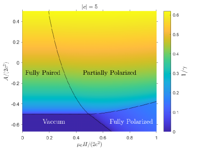
(a) $1/\gamma$

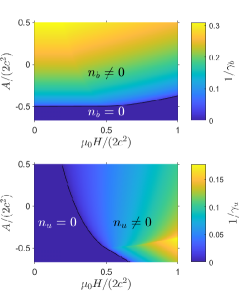
(b) $1/\gamma_{b}$ and $1/\gamma_{u}$

Figure 6: Phase diagrams represented by dimensionless particle densities $1/\gamma$, $1/\gamma_{b}$ and $1/\gamma_{u}$. Here dimensionless quantities $A/(2c^{2})$ and $\mu_{0}H/(2c^{2})$ are used as variables, where $2c^{2}$ is the binding energy. The black lines indicate the phase boundaries, which are obtained from the two diagrams in (a). For the partially polarized phase, the strong coupling $\gamma\gg 1$ near the quartet point. Clearly, according to (b), the boundaries of each phase (black lines) in (a) are given at the boundaries of zero- or nonzero-particle densities of paired and unpaired sections. The phase boundaries in (a) can also be determined by Eq. (15).

IV Analytical Results

IV.1 Strong Coupling Limit in Partially Polarized Phase

In general, analytical expressions of physical quantities are hardly obtained from the BA equations unless in certain extreme limits. Usually, one consider the weak and strong coupling limits, $\left|c\right|\ll n$ and $\left|c\right|\gg n$ in 1D ultracold atomic systems. The coupling strength $\left|c\right|/n$ can be experimentally tuned from weak to strong by controlling the 3D scattering length near the Feshbach resonance, i.e.

$$\frac{c^{2}}{n^{2}}=\frac{mg_{1\mathrm{D}}^{2}}{8\hbar^{2}n^{2}}\text{, and }g_{1\mathrm{D}}=\frac{2\hbar^{2}a_{3\mathrm{D}}}{ma_{\perp}^{2}}\frac{1}{1-Aa_{3\mathrm{D}}/a_{\perp}},$$ (27)

where $g_{1\mathrm{D}}$ is the effective inter-component interaction, $a_{3\mathrm{D}}$ is the 3D scattering length, $a_{\perp}$ is the transverse oscillator length. For our convenience, we denote the dimensionless coupling strengths $\gamma=\left|c\right|/n$, $\gamma_{b}=\left|c\right|/n_{b}$, and $\gamma_{u}=\left|c\right|/n_{u}$. What below are the derivations of analytical results of physical quantities for the strong coupling regime, $\gamma\gg 1$.

In the grand canonical ensemble, quantum phase transitions take place at zero-temperature, which have already been studied in both the canonical ensemble and the grand canonical ensemble orso2007attractive ; hu2007phase ; guan2011quantum ; yin2011quantum . Here we discuss analytical results in the grand canonical ensemble, where the parameters $\{c,A,\mu_{0}H\}$ are our driving parameters. For example, the phase digram and interaction strengths can be given in $\mu-H$ plane, see Fig. 6 and Fig. 7.

From Fig. 6, we observe that the strong coupling $\gamma\gg 1$ (regions plotted in dark-blue) can be reached in the vicinity of the edge of the vacuum phase. In the partially polarized (FFLO-like) phase, the strong coupling regime locates near the quartet point $A/c^{2}=-1$ and $\mu_{0}H/c^{2}=1$. If we define the effective chemical potentials of both sector $A_{b}=A+c^{2}$ and $A_{u}=A+\mu_{0}H$, the strong coupling regime meets the condition $A_{b}\ll c^{2}$ and $A_{u}\ll c^{2}$.

In Fig. 7 (a), we plot the polarization in the $\mu-H$ plane for fixed value of interaction strength. From 7 (b), we observe the polarization $P=n_{u}/(2n_{b}+n_{u})$ varies drastically in the vicinity of the quartet point. Therefore, it might come into the expression of the band curvature corrections of sound velocities and effective masses for the strong coupling.

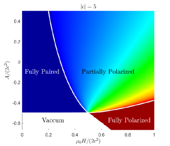
(a) polarization

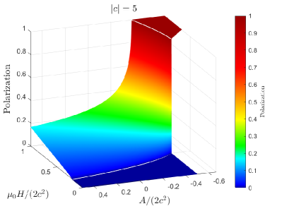
(b) polarization in 3D-version

Figure 7: Phase diagram is represented by polarization. In (a), the white lines give the phase boundaries. In (b), The polarization varies drastically in the vicinity of the quartet point.

IV.2 Sound Velocity and Effective Mass in One-Particle-hole Excitation Spectrum

In this section, we will derive the exact dispersions of particle-hole excitations in both paired and unpaired fermions. We first derive the dispersion of bound pairs in the long-wavelength limit, i.e., we derive the linear dispersion with a curvature correction. Consequently, we can obtain the sound velocities and effective masses in terms of dressed energies and the density distribution functions. For a one-particle-hole excitation near the Fermi point $B$ of the bound pairs, the excited energy and momentum are given by

$$\Delta E_{b}= \varepsilon\left(k_{p,i}\right)-\varepsilon\left(k_{h,i}\right)=\varepsilon\left(B+\Delta k\right)-\varepsilon\left(B\right),$$ (28)

$$\Delta K_{b}= 2\pi\left[\int_{0}^{k_{p,i}}\sigma\left(k\right)\mathrm{d}k-\int_{0}^{k_{h,i}}\sigma\left(k\right)\mathrm{d}k\right]=2\pi\left[\int_{0}^{B+\Delta k}\sigma\left(k\right)\mathrm{d}k-\int_{0}^{B}\sigma\left(k\right)\mathrm{d}k\right].$$

In the long-wavelength limit, the excitation is near the Fermi point, i.e., $\Delta k\ll 1$. Therefore, the excited energy and momentum can be expanded at $k=B$. Namely,

$$\Delta E_{b} \approx \varepsilon\left(B\right)+\varepsilon^{\prime}\left(B\right)\Delta k+\frac{\varepsilon^{\prime\prime}\left(B\right)}{2}\left(\Delta k\right)^{2}=\varepsilon^{\prime}\left(B\right)\Delta k+\frac{\varepsilon^{\prime\prime}\left(B\right)}{2}\left(\Delta k\right)^{2},$$ (29)

$$\Delta K_{b} \approx 2\pi\int_{0}^{B}\sigma\left(k\right)\mathrm{d}k+2\pi\sigma\left(B\right)\Delta k+2\pi\frac{\sigma^{\prime}\left(B\right)}{2}\left(\Delta k\right)^{2}-2\pi\int_{0}^{B}\sigma\left(k\right)\mathrm{d}k$$ (30)

$$= 2\pi\sigma\left(B\right)\Delta k+2\pi\frac{\sigma^{\prime}\left(B\right)}{2}\left(\Delta k\right)^{2},$$

where $f^{\prime}(x)$ and $f^{\prime\prime}(x)$ denote the first- and second-order derivatives of $f(x)$ with respect to $x$, respectively. From the relation

$$\Delta K_{b}=2\pi\sigma\left(B\right)\Delta k\left(1+\frac{\sigma^{\prime}\left(B\right)}{2\sigma\left(B\right)}\Delta k\right),$$

we directly obtain $\Delta k$,

$$\Delta k\approx\frac{1}{2\pi\sigma(B)}\Delta K_{b}-\frac{\sigma^{\prime}\left(B\right)}{8\pi^{2}\left(\sigma\left(B\right)\right)^{3}}\left(\Delta K_{b}\right)^{2}.$$ (31)

Subsequently, we have the following dispersion relation for the bound pairs

$$\Delta E_{b} \approx\varepsilon(B)\left(\frac{1}{2\pi\sigma(B)}\Delta K_{b}-\frac{\sigma^{\prime}\left(B\right)}{8\pi^{2}\left(\sigma\left(B\right)\right)^{3}}\left(\Delta K_{b}\right)^{2}\right)+\frac{\varepsilon^{\prime\prime}(B)}{2}\left(\frac{1}{2\pi\sigma(B)}\Delta K_{b}\right)^{2}$$ (32)

$$\approx\frac{\varepsilon^{\prime}(B)}{2\pi\sigma(B)}\Delta K_{b}+\left[\frac{\varepsilon^{\prime\prime}(B)}{8\pi^{2}\left(\sigma(B)\right)^{2}}-\frac{\sigma^{\prime}(B)\varepsilon^{\prime}(B)}{8\pi^{2}\left(\sigma(B)\right)^{3}}\right](\Delta K_{b})^{2}$$

$$\approx 2\left[v_{b}\frac{\Delta K_{b}}{2}+\frac{1}{2m^{*}_{b}}\left(\frac{\Delta K_{b}}{2}\right)^{2}\right]$$

expressed up to the second-order of $\Delta K_{b}$. From this relation, we read off the sound velocity and effective mass of the one-particle-hole excitation in the paired Fermi sea as

$$v_{b} =\frac{\varepsilon^{\prime}(B)}{2\pi\sigma(B)},$$ (33)

$$\frac{1}{4m^{*}_{b}} =\frac{\varepsilon^{\prime\prime}(B)}{8\pi^{2}\left(\sigma(B)\right)^{2}}-\frac{\sigma^{\prime}(B)\varepsilon^{\prime}(B)}{8\pi^{2}\left(\sigma(B)\right)^{3}},$$

which hold true for arbitrary coupling strength and thus will be used in our numerical calculations.

Similarly, a one-particle-hole excitation for unpaired fermions near the Fermi point can be calculated via the excited energy and momentum,

$$\Delta E_{u}= \left[\kappa\left(k_{p,i}\right)-\kappa\left(k_{h,i}\right)\right]=\left[\kappa\left(Q+\Delta k\right)-\kappa\left(Q\right)\right]\approx\kappa^{\prime}\left(Q\right)\Delta k+\frac{\kappa^{\prime\prime}\left(Q\right)}{2}\left(\Delta k\right)^{2},$$ (34)

$$\Delta K_{u}= 2\pi\left[\int_{0}^{k_{p,i}}\rho\left(k\right)\mathrm{d}k-\int_{0}^{k_{h,i}}\rho\left(k\right)\mathrm{d}k\right]=2\pi\left[\int_{0}^{Q+\Delta k}\rho\left(k\right)\mathrm{d}k-\int_{0}^{Q}\rho\left(k\right)\mathrm{d}k\right]$$

$$\approx 2\pi\rho\left(Q\right)\Delta k+2\pi\frac{\rho^{\prime}\left(Q\right)}{2}\left(\Delta k\right)^{2}.$$

The excited energy can be expressed by the excited momentum as well as Eq.(32),

$$\Delta E_{u} =\kappa(Q)\left(\frac{1}{2\pi\rho(Q)}\Delta K_{u}-\frac{\rho^{\prime}(Q)}{8\pi^{2}\left(\rho(Q)\right)^{3}}\left(\Delta K_{u}\right)^{2}\right)+\frac{\kappa^{\prime\prime}(Q)}{2}\left(\frac{1}{2\pi\rho(Q)}\Delta K_{u}\right)^{2}$$ (35)

$$=\frac{\kappa^{\prime}(Q)}{2\pi\rho(Q)}\Delta K_{u}+\left[\frac{\kappa^{\prime\prime}(Q)}{8\pi^{2}\left(\rho(Q)\right)^{2}}-\frac{\rho^{\prime}(Q)\kappa^{\prime}(Q)}{8\pi^{2}\left(\rho(Q)\right)^{3}}\right](\Delta K_{u})^{2}=v_{u}\Delta K_{u}+\frac{1}{2m^{*}_{b}}\left(\Delta K_{u}\right)^{2}.$$

Therefore, by comparison, the sound velocity and effective mass of the one-particle-hole excitation in the unpaired Fermi sea are given by

$$v_{u} =\frac{\kappa^{\prime}(Q)}{2\pi\rho(Q)},$$ (36)

$$\frac{1}{2m^{*}_{u}} =\frac{\kappa^{\prime\prime}(Q)}{8\pi^{2}\left(\rho(Q)\right)^{2}}-\frac{\rho^{\prime}(Q)\kappa^{\prime}(Q)}{8\pi^{2}\left(\rho(Q)\right)^{3}}.$$

The obtained relations for velocities and effective masses (33) and (36) are very convenient to carry out numerical calculations, see Fig. 4.

For a strong coupling, i.e. $|c|\gg 1$, we may directly use the dressed energies Eq.(15) and the distribution functions Eq.(17) to determine the dispersion relations characterized by the sound velocities and effective masses. To this end, we first calculate Fermi momenta $B$ and $Q$ in terms of particle densities $n_{u}$, $n_{b}$ with our chose parameters $\{c,A,\mu_{0}H\}$ (i.e., $[A_{b},A_{u}]$). For the strong coupling, we may expand the kernels $a_{1}(k)$ and $a_{2}(k)$ up to the first order of $1/c$, the distribution functions Eq.(17) thus become

$$\sigma\left(k\right)\approx\frac{1}{\pi}-a_{2}\left(k\right)\int_{-B}^{B}\sigma\left(k^{\prime}\right)\mathrm{d}k^{\prime}-a_{1}\left(k\right)\int_{-Q}^{Q}\rho\left(k^{\prime}\right)\mathrm{d}k^{\prime}=\frac{1}{\pi}-a_{2}\left(k\right)n_{b}-a_{1}\left(k\right)n_{u},$$ (37)

$$\rho\left(k\right)\approx\frac{1}{2\pi}-a_{1}\left(k\right)\int_{-B}^{B}\sigma\left(k^{\prime}\right)\mathrm{d}k^{\prime}=\frac{1}{2\pi}-a_{1}\left(k\right)n_{b}.$$

The paiticle densities $n_{b}$ and $n_{u}$ are related to Fermi momenta $B$ and $Q$ via

$$n_{b} =\int_{-B}^{B}\sigma\left(k\right)\mathrm{d}k\approx\int_{-B}^{B}\left(\frac{1}{\pi}-a_{2}\left(k\right)n_{b}-a_{1}\left(k\right)n_{u}\right)\mathrm{d}k$$ (38)

$$=\frac{2B}{\pi}-\frac{2}{\pi}\arctan{\frac{B}{2\left|c\right|}}n_{b}-\frac{2}{\pi}\arctan{\frac{B}{\left|c\right|}}n_{u}\approx\frac{2B}{\pi}\left(1-\frac{B}{\pi\left|c\right|}-\frac{Q}{\pi\left|c\right|}\right),$$

$$n_{u} =\int_{-Q}^{Q}\rho\left(k\right)\mathrm{d}k\approx\int_{-Q}^{Q}\left(\frac{1}{2\pi}-a_{1}\left(k\right)n_{b}\right)\mathrm{d}k=\frac{Q}{\pi}-\frac{2}{\pi}\arctan{\frac{Q}{\left|c\right|}}n_{b}\approx\frac{Q}{\pi}\left(1-\frac{4B}{\pi\left|c\right|}\right),$$

which suggest the following relations between particle densities ($n_{u}$ and $n_{b}$) and Fermi momenta ($B$ and $Q$)

$$B=\frac{1}{2}\pi n_{b}\left(1-\frac{B}{\pi\left|c\right|}-\frac{Q}{\pi\left|c\right|}\right)^{-1}\approx\frac{1}{2}\pi n_{b}\left(1+\frac{B+Q}{\pi\left|c\right|}\right),$$ (39)

$$Q=\pi n_{u}\left(1-\frac{4B}{\pi\left|c\right|}\right)^{-1}\approx\pi n_{u}\left(1+\frac{4B}{\pi\left|c\right|}\right).$$

For a further derivation of the velocities, we need the effective chemical pressures of pairs and unpaired fermions

$$p_{b}=-\frac{1}{\pi}\int_{-B}^{B}\varepsilon(k)\mathrm{d}k,\quad p_{u}=-\frac{1}{2\pi}\int_{-Q}^{Q}\kappa(k)\mathrm{d}k.$$ (40)

From the dressed energy Eq.(15), we may obtain the following relations between effective chemical potentials and Fermi momenta guan2007phase

$$B^{2}\approx A+c^{2}-\frac{p_{b}+4p_{u}}{4\left|c\right|}=A_{b}-\frac{p_{b}+4p_{u}}{4\left|c\right|},\quad Q^{2}\approx A+\mu_{0}H-\frac{p_{b}}{\left|c\right|}=A_{u}-\frac{p_{b}}{\left|c\right|}.$$ (41)

Consequently, according to Eqs.(39) and (41), we built up the relations between the particle densities and our chosen parameters $\{c,A,\mu_{0}H\}$ through the Fermi point $B$ and $Q$.

Now we can rewrite the expressions of the sound velocities and effective masses following the expressions Eq.(33) and (36) for the strong coupling regime. To determine $v_{b}$ and $m_{b}^{*}$ given by Eq.(33), we first calculate $\varepsilon^{\prime}(B)$ and $\sigma(B)$ and their derivatives. According to Eq.(15), $\varepsilon^{\prime}(B)$ is given by

$$\varepsilon^{\prime}\left(B\right)=4B-\int_{-B}^{B}\left.\frac{\mathrm{d}a_{2}\left(k-k^{\prime}\right)}{\mathrm{d}k}\right|_{k=B}\varepsilon\left(k^{\prime}\right)\mathrm{d}k^{\prime}-\int_{-Q}^{Q}\left.\frac{\mathrm{d}a_{1}\left(k-k^{\prime}\right)}{\mathrm{d}k}\right|_{k=B}\kappa\left(k^{\prime}\right)\mathrm{d}k^{\prime}\approx 4B,$$ (42)

where we ignored the order $1/c^{2}$, for example, the leading order of $\mathrm{d}a_{n}(k)/\mathrm{d}k$ is $\mathcal{O}(1/c^{3})$ in the strong coupling limit. Similarly, we can have $\varepsilon^{\prime\prime}\left(B\right)=4+\mathcal{O}(1/c^{4})$. Whereas the distribution function $\sigma\left(B\right)$ can be obtained by substituting Eqs.(37) into Eq.(17), namely,

$$\sigma\left(B\right)$$ (43)

$$= \frac{1}{\pi}-\int_{-B}^{B}a_{2}\left(B-k^{\prime}\right)\left(\frac{1}{\pi}-a_{2}\left(k^{\prime}\right)n_{b}-a_{1}\left(k^{\prime}\right)n_{u}\right)\mathrm{d}k^{\prime}-\int_{-Q}^{Q}a_{1}\left(B-k^{\prime}\right)\left(\frac{1}{2\pi}-a_{1}\left(k^{\prime}\right)n_{b}\right)\mathrm{d}k^{\prime}$$

$$\approx \frac{1}{\pi}-\frac{1}{\pi}\int_{-B}^{B}\frac{1}{2\pi\left|c\right|}\mathrm{d}k^{\prime}-\frac{1}{2\pi}\int_{-Q}^{Q}\frac{1}{\pi\left|c\right|}\mathrm{d}k^{\prime}\approx\frac{1}{\pi}\left(1-\frac{B+Q}{\pi\left|c\right|}\right).$$

While its derivative $\sigma^{\prime}\left(B\right)\sim\mathcal{O}\left(1/c^{3}\right)$ is negligible. By substituting $\varepsilon^{\prime}(B)$ and $\sigma(B)$ and their derivatives into Eq.(33), we may express $v_{b}$ and $m_{b}^{*}$ with respect to Fermi momenta $B$ and $Q$

$$v_{b}=\frac{\varepsilon^{\prime}(B)}{2\pi\sigma(B)}=2B\left(1-\frac{B+Q}{\pi\left|c\right|}\right)^{-1}\approx 2B\left(1+\frac{B+Q}{\pi\left|c\right|}\right),$$ (44)

$$\frac{1}{4m^{*}_{b}}=\frac{\varepsilon^{\prime\prime}(B)}{8\pi^{2}\left(\sigma(B)\right)^{2}}-\frac{\sigma^{\prime}(B)\varepsilon^{\prime}(B)}{8\pi^{2}\left(\sigma(B)\right)^{3}}\approx\frac{1}{2}\left(1-\frac{B+Q}{\pi\left|c\right|}\right)^{-2}.$$

By substituting Eqs.(39) into the last equations, we further express $v_{b}$ and $m_{b}^{*}$ in $\gamma_{b}$ and $\gamma_{u}$

$$v_{b} \approx\pi n_{b}\left(1+\frac{B+Q}{\pi\left|c\right|}\right)^{2}\approx\pi n_{b}\left(1+\frac{2B+2Q}{\pi\left|c\right|}\right)\approx\pi n_{b}\left(1+\frac{1}{\gamma_{b}}+\frac{2}{\gamma_{u}}\right),$$ (45)

$$m^{*}_{b} \approx\frac{1}{2}\left(1-\frac{B+Q}{\pi\left|c\right|}\right)^{-2}\approx\frac{1}{2}\left(1+\frac{2B+2Q}{\pi\left|c\right|}\right)=m_{b}\left(1+\frac{2B+2Q}{\pi\left|c\right|}\right)\approx m_{b}\left(1-\frac{1}{\gamma_{b}}-\frac{2}{\gamma_{u}}\right).$$

Similarly, we may obtain $v_{u}$ and $m_{u}^{*}$ from Eq.(36). The terms $\kappa^{\prime}(Q)$ and $\rho(Q)$ are given by

$$\kappa^{\prime}(Q)=2Q, \kappa^{\prime\prime}(Q) =2,$$ (46)

$$\rho(Q)=\frac{1}{2\pi}\left(1-\frac{4B}{\pi\left|c\right|}\right),\quad \rho^{\prime}(Q) \sim\mathcal{O}\left(\frac{1}{c^{3}}\right)$$

up to the order of $1/c^{2}$. Substituting them into Eqs.(36), we obtain $v_{u}$ and $m_{u}^{*}$ in the following forms

$$v_{u} \approx 2\pi n_{u}\left(1+\frac{4B}{\pi\left|c\right|}\right)^{2}\approx 2\pi n_{u}\left(1+\frac{8B}{\pi\left|c\right|}\right)\approx 2\pi n_{u}\left(1+\frac{4}{\gamma_{b}}\right),$$ (47)

$$m^{*}_{u} \approx\left(1-\frac{4B}{\pi\left|c\right|}\right)^{-2}\approx\left(1+\frac{8B}{\pi\left|c\right|}\right)=m\left(1+\frac{8B}{\pi\left|c\right|}\right)\approx m\left(1-\frac{4}{\gamma_{b}}\right).$$

Furthermore, owing to Eqs.(39) and (41), we replace $\gamma_{b}$ and $\gamma_{u}$ in Eqs.(45) and (47) by $\gamma$ and the polarization $P$ or the ratio between two effective chemical potentials $A_{b}$ and $A_{u}$. Since the polarization is defined by $P=n_{u}/n$, we have $\gamma/\gamma_{b}=n_{b}/n=(1-P)/2$ and $\gamma/\gamma_{u}=n_{u}/n=P$, which allows us to express the sound velocities and effective masses as a function of $P$. Alternatively, we would like to express the sound velocities and effective masses in terms of $A_{b}$ and $A_{u}$. Since they are directly related to our controllable parameters $\{c,A,\mu_{0}H\}$. According to Eqs.(39) and (41), we have

$$\left(\frac{Q}{B}\right)^{2}\approx\left(\frac{2n_{u}}{n_{b}}\right)^{2}=4\left(\frac{2P}{1-P}\right)^{2}\approx\frac{A_{u}}{A_{b}}=\alpha^{2}.$$ (48)

We denote the ratio of effective chemical potential as $A_{u}/A_{b}=\alpha^{2}$ for our convenience in analysis. Using the polarization $P$ and the ratio $\alpha$, we can rewrite Eqs.(45) and (47) as

$$v_{b}\approx\pi n_{b}\left(1+\left(1+3P\right)\frac{1}{2\gamma}\right)\approx\pi n_{b}\left(1+\frac{2+2\alpha}{4+\alpha}\frac{1}{\gamma}\right),$$ (49)

$$v_{u}\approx 2\pi n_{u}\left(1+\left(2-2P\right)\frac{1}{\gamma}\right)\approx 2\pi n_{u}\left(1+\frac{8}{4+\alpha}\frac{1}{\gamma}\right),$$

$$m^{*}_{b}\approx m_{b}\left(1-\left(1+3P\right)\frac{1}{2\gamma}\right)\approx m_{b}\left(1-\frac{2+2\alpha}{4+\alpha}\frac{1}{\gamma}\right),$$

$$m^{*}_{u}\approx m_{u}\left(1-\left(2-2P\right)\frac{1}{\gamma}\right)\approx m_{u}\left(1-\frac{8}{4+\alpha}\frac{1}{\gamma}\right),$$

which are confirmed by numerical results in Fig. 8, where we set the polarization $P=1/5$ (i.e., $\alpha=1$). According to Eq.(48) and the last equations Eqs (49), the ratio between two sound velocities is simply given by $v_{u}/v_{b}=2n_{u}/n_{b}=\alpha$ up to the order of $1/c^{2}$, which provides physical insight into the sound velocities in Fig. 5, where our chosen parameters $\{c,A,\mu_{0}H\}$ indicate a strong coupling with $\alpha=2$ and $\alpha=1$, respectively. Furthermore, since $k_{F,b}\approx\pi n_{b}$ and $k_{F,u}\approx\pi n_{u}$ (illustrated at the end of Section III.1), we have $k_{F,u}/k_{F,b}=\alpha/2$, which gives a special ratio between two Fermi points in Fig. 5.

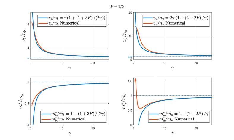
Figure 8: Variation of sound velocities, $v_{b}$ and $v_{u}$, and effective masses, $m^{*}_{b}$ and $m^{*}_{u}$ v.s. the dimensionless interaction strengths $\gamma$. The polarization is fixed to be $P=1/5$ with $\gamma=10$. The analytical (blue) Eq.(49) are agreeable with the numerical (red) results which are plotted with respect to Eqs.(33) and (36).

So far, we derived the sound velocities and effective masses of paired and unpaired fermions starting from the zero-temperature TBA equations. For the repulsive case, it is provedhe2020emergence that these quantities can be derived from the BA equations; by a similar method, one can prove that this works for the attractive case as well (See Appendix.SM6.2 for detailed procedure). This is reasonable since the TBA equations are derived from the BA equations.

The sound velocities and effective masses can effectively characterize the spectra of one-particle-hole excitation. Therefore, these quantities can be regarded as evidence and provide convenience to varify the separation of collective motions within paired and unpaired charges at zero temperature. This kind of charge-charge separation can even be characterized at non-zero but low temperature. According to the relations given by Eqs.(33) and (36), the zero-temperature subtraction for low-temperature free energy density can be expressed by (see Appendix.SM6.3 for proof)

$$\Omega/L-\Omega_{0}/L=p-p_{0}=\frac{\pi T^{2}}{6}\left(\frac{1}{v_{b}}+\frac{1}{v_{u}}\right),$$ (50)

which is simply the addition of contribution of paired and unpaired sections. This additivity manifests the independent character and separation of paired and unpaired bosonic modes. Moreover, the $T^{2}$ dependence given by the low-temperature pressure correction shows a typical linear dispersions feature. The specific heat can also be obtained by its definition, i.e.,

$$c_{V}=T\frac{\partial^{2}p}{\partial T^{2}}=\frac{\pi T}{3}\left(\frac{1}{v_{b}}+\frac{1}{v_{u}}\right),$$ (51)

which preserves the additivity and describes the novel charge-charge separation as well at low temperature.

V Excitations other than single particle-hole

In this section, we will consider excitations other than the one particle-hole excitation, such as excitations of multiple particle-holes, breaking and forming pairs, as well as length-$n$ string excitations.

V.1 Multiple particle-hole Excitations

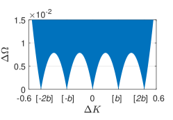
(a) $N_{b}=2$, $N_{u}=0$

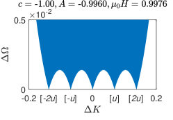
(b) $N_{b}=0$, $N_{u}=2$

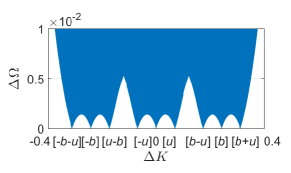
(c) $N_{b}=1$, $N_{u}=1$

Figure 9: Two-particle-hole excitations spectra. The numbers of excited particle-holes in paired and unpaired sectors. The figures (a), (b) and (c) show particle-hole excitations for different $N_{b}$ and $N_{u}$. Here we denote $[\alpha b+\beta u]\equiv:2\left(\alpha k_{F,b}+\beta k_{F,u}\right)$. In this figure, we set $c=-1.00$, $A=-0.9960$, $\mu_{0}H=0.9976$ for our numerical calculation with the dispersions represented by Eq.(52)

In the case of exciting $N_{b}$ paired fermions and $N_{u}$ unpaired fermions, like what we did in Eq.(22), introducing $2N_{b}+2N_{u}$ $\delta$-functions, $\sum_{i=1}^{N_{b}}[-\delta\left(k-k_{h,i}\right)+\delta\left(k-k_{p,i}\right)]/L+\sum_{j=1}^{N_{u}}[-\delta\left(k-\right.$ $\left.k_{h,j}\right)+\delta\left(k-k_{p,j}\right)]/L$ into the distribution functions Eq.(17), one can prove that the excitation energy momentum are given by their summation of one-particle-hole excitation ones, respectively

$$\Delta\Omega= \sum_{i=1}^{N_{b}}\left[\varepsilon^{0}\left(\lambda_{p,i}\right)-\varepsilon^{0}\left(\lambda_{h,i}\right)\right]+\sum_{i=1}^{N_{u}}\left[\kappa^{0}\left(k_{p,i}\right)-\kappa^{0}\left(k_{h,i}\right)\right]$$ (52)

$$\Delta K= 2\pi\sum_{i=1}^{N_{b}}\left[\int_{0}^{\lambda_{p,i}}\sigma^{0}\left(k\right)\mathrm{d}k-\int_{0}^{\lambda_{h,i}}\sigma^{0}\left(k\right)\mathrm{d}k\right]+2\pi\sum_{i=1}^{N_{u}}\left[\int_{0}^{k_{p,i}}\rho^{0}\left(k\right)\mathrm{d}k-\int_{0}^{k_{h,i}}\rho^{0}\left(k\right)\mathrm{d}k\right].$$

The calculation is essentially similar as that for one-particle-hole dispersion. Here we do not wish to present the calculation in detail. Fig. 9 shows three examples for various choices of the numbers $N_{b}$ and $N_{u}$.

V.2 Excitations by pairing and depairing without exciting any n-string

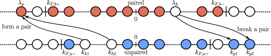
Figure 10: Schematic illustration of forming or breaking a pair.

For the case of breaking $N_{ub}$ pairs, we create $N_{ub}$ holes in the paired Fermi sea while add $2N_{ub}$ fermions in the unpaired sea, see Fig. 10. For the case of forming $N_{bu}$ pairs, we create $2N_{bu}$ holes in the unpaired Fermi sea and add $N_{bu}$ pairs in the paired Fermi. In comparison with the ground state, for breaking $N_{ub}$ pairs, while forming $N_{bu}$ pairs, the particle numbers are given by

$$N=N_{G},\quad M=M_{G}-N_{ub}+N_{bu},\quad M_{n}=0,\text{ for }n=1,2,\cdots.$$

We introduce $\delta$-functions for representing the excited pairs and unpaired particles and holes as

$$-\sum_{i=1}^{N_{ub}}\delta\left(k-\lambda_{h,i}\right)/L+\sum_{i=1}^{N_{ub}}\left[\delta\left(k-k_{p1,i}\right)/L+\delta\left(k-k_{p2,i}\right)/L\right]\text{ (for breaking $N_{ub}$ pairs) }$$ (53)

$$+\sum_{i=1}^{N_{bu}}\delta\left(k-\lambda_{p,i}\right)/L-\sum_{i=1}^{N_{bu}}\left[\delta\left(k-k_{h1,i}\right)/L+\delta\left(k-k_{h2,i}\right)/L\right]\text{ (for forming $N_{bu}$ pairs)},$$

respectively, where $k_{p1,i}$, $k_{p2,i}$, $k_{h1,i}$, and $k_{h2,i}$ stand for the excited quasimomenta of unpaired particles and holes. As we did in Eq.(22), substitute the $\delta$-funciotns(53) into the distribution functions Eq.(17). By taking similar calculation to that of the single particle-hole excitation, the excited energy of multiple pair- forming and breaking is given by

$$\Delta\Omega= \int_{Q_{-}}^{Q_{+}}\rho\left(k\right)\left(k^{2}-\mu_{0}H\right)\mathrm{d}k-\int_{-Q_{0}}^{Q_{0}}\rho^{0}\left(k\right)\left(k^{2}-\mu_{0}H\right)\mathrm{d}k$$ (54)

$$+2\int_{B_{-}}^{B_{+}}\sigma\left(\lambda\right)\left(\lambda^{2}-c^{2}\right)\mathrm{d}\lambda-2\int_{-B_{0}}^{B_{0}}\sigma\left(\lambda\right)\left(\lambda^{2}-c^{2}\right)\mathrm{d}\lambda$$

$$= \sum_{i=1}^{N_{ub}}\left[\kappa^{0}\left(k_{p1,i}\right)+\kappa^{0}\left(k_{p2,i}\right)-\varepsilon^{0}\left(\lambda_{h,i}\right)\right]+\sum_{i=1}^{N_{bu}}\left[\varepsilon^{0}\left(\lambda_{p,i}\right)-\kappa^{0}\left(k_{h1,i}\right)-\kappa^{0}\left(k_{h2,i}\right)\right]\textcolor{blue}{.}$$

The total momentum for this excitation, depends on not only the quasimomenta of exited holes and particles, but also the numbers of breaking pairs and forming pairs $N_{ub}$ and $N_{bu}$. The parity of quasimomenta of pairs in such a type of excitations does not change because it only depends on $N=N_{G}$ (see Eq.(19)). Meanwhile the parity of quasimomenta of unpaired fermions is changed since it depends on $N+M=N_{G}+M_{G}-N_{ub}+N_{bu}$. Therefore, an additional phase shift is caused due to the change of parity, namely,

$$\Delta K= 2\pi\sum_{i=1}^{N_{ub}}\left[\left(\int_{0}^{k_{p1,i}}+\int_{0}^{k_{p2,i}}\right)\rho^{0}\left(k\right)\mathrm{d}k-\int_{0}^{\lambda_{h,i}}\sigma^{0}\left(k\right)\mathrm{d}k\right]$$ (55)

$$+2\pi\sum_{i=1}^{N_{bu}}\left[\int_{0}^{\lambda_{p,i}}\sigma^{0}\left(k\right)\mathrm{d}k-\left(\int_{0}^{k_{h1,i}}+\int_{0}^{k_{h2,i}}\right)\rho^{0}\left(k\right)\mathrm{d}k\right]\pm\begin{cases}0&,\text{for $N_{ub}-N_{bu}$ even}\\ \pi n_{u}&,\text{for $N_{ub}-N_{bu}$ odd}\end{cases}.$$

We see that odd $\{N_{ub}-N_{bu}\}$ gives a two-fold-degenerate excited state. In Fig. 11 we present excitation spectra of breaking or forming one pair. Obviously, the spectra are more complicated due to the two-fold degeneracy.

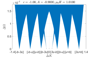
(a) breaking one pair

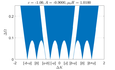
(b) forming one pair

Figure 11: Excited spectrum of breaking or forming one pair. The excitation spectra show two-fold degeneracy in breaking a pair and forming a pair. Here we denote $[\alpha b+\beta u]\equiv:2\left(\alpha k_{F,b}+\beta k_{F,u}\right)$. We set $c=-1.00$, $A=-0.9000$, $\mu_{0}H=1.0100$ for our numerical calculation with the dispersions Eqs.(54) and (55).

V.3 n-strings Excitations

Now we consider excitations by flipping spins in the unpaired fermions without forming pairs. According to Eq.(12), the dressed energy and distribution function in the spin sector at the ground state are given by

$$\varepsilon_{n}^{0}\left(\lambda\right)=2n\mu_{0}H-\int_{-Q_{0}}^{Q_{0}}a_{n}\left(\lambda-k^{\prime}\right)\kappa^{0}\left(k^{\prime}\right)\mathrm{d}k^{\prime},\quad\sigma_{n}^{0}\left(\lambda\right)=\sigma_{n}^{0}{}^{h}\left(\lambda\right)=\int_{-Q_{0}}^{Q_{0}}a_{n}\left(\lambda-k^{\prime}\right)\rho^{0}\left(k^{\prime}\right)\mathrm{d}k^{\prime}.$$ (56)

For the ground state, all spin strings are unoccupied at the zero temperature. The dressed energies and distribution functions for $n$-strings with $n=1,2,3$ are plotted in Fig. 12a.

For simplicity, consider the case of exciting one length-$l$ string by flipping unpaired fermions, i.e., $M_{l}=M_{l,G}+1=1$ and $M_{n}=0$ for $n\neq l$. The quantum numbers of the spin setor $J_{\alpha}{}^{n}$ are integer (half-odd integer) for $N-M_{n}$ odd (even), and satisfy Eq.(7). Therefore, for the ground state, $J_{\alpha}{}^{n}$ are confined by the condition

$$\left|J_{\alpha}{}^{n}\right|\leqq\left(N-2M\right)/2,$$ (57)

which indicates $N-2M$ holes and no occupation of all $n$-strings. For the excited state with $M_{\ell}=1$, $J_{\alpha}{}^{n}$ are confined by the condition

$$\left|J_{\alpha}{}^{n}\right|\leqq\begin{cases}\left(N-2M-2n\right)/2&,n<\ell,\vspace{5pt}\\ \left(N-2M-2\ell+1\right)/2&,n=\ell,\vspace{5pt}\\ \left(N-2M-2\ell\right)/2&,n>\ell,\end{cases}$$ (58)

that indicates $N-2M-2n$ holes for $n\leq\ell$, $N-2M-2\ell$ holes for $n>\ell$ and one occupation of length-$\ell$ string for $n=\ell$. By introduce $\delta\left(k-\lambda_{\ell}\right)/L$ representing the excited $\ell$-string into the distribution functions, we have

$$\bar{\sigma}\left(k\right)=\frac{1}{\pi}-\int_{-B}^{B}a_{2}\left(k-k^{\prime}\right)\sigma\left(k^{\prime}\right)\mathrm{d}k^{\prime}-\int_{-Q}^{Q}a_{1}\left(k-k^{\prime}\right)\rho\left(k^{\prime}\right)\mathrm{d}k^{\prime},$$ (59)

$$\bar{\rho}\left(k\right)=\frac{1}{2\pi}-\int_{-B}^{B}a_{1}\left(k-k^{\prime}\right)\sigma\left(k^{\prime}\right)\mathrm{d}k^{\prime}-\int_{-B_{n}}^{B_{n}}a_{\ell}\left(k-k^{\prime}\right)\bar{\sigma}_{l}\left(k^{\prime}\right)\mathrm{d}k^{\prime}+\frac{1}{L}a_{\ell}\left(k-\lambda_{\ell}\right),$$

$$\bar{\sigma}_{n}\left(k\right)=\int_{-Q}^{Q}a_{n}\left(k-k^{\prime}\right)\rho\left(k^{\prime}\right)\mathrm{d}k^{\prime},$$

where we denoted $\bar{\sigma}_{n}=\sigma_{n}+\sigma_{n}^{h}$, and we define $B_{n}$ by $\bar{\sigma}_{n}(B_{n})=0$. The excited free energy density is thus given by

$$\frac{\Delta\Omega}{L}= \int_{Q_{-}}^{Q_{+}}{\rho}\left(k\right)\left(k^{2}-\mu_{0}H\right)\mathrm{d}k+2\int_{B_{-}}^{B_{+}}{\sigma}\left(k\right)\left(k^{2}-c^{2}\right)\mathrm{d}k+\sum_{n=1}^{\infty}2n\mu_{0}H\int_{B_{n+}}^{B_{n-}}\sigma_{n}\left(k\right)\mathrm{d}k$$ (60)

$$-\int_{-Q_{0}}^{Q_{0}}\rho^{0}\left(k\right)\left(k^{2}-\mu_{0}H\right)\mathrm{d}k-2\int_{-B_{0}}^{B_{0}}\sigma^{0}\left(k\right)\left(k^{2}-c^{2}\right)\mathrm{d}k-\sum_{n=1}^{\infty}2n\mu_{0}H\int_{B_{n0}}^{B_{n0}}\sigma_{n}^{0}\left(k\right)\mathrm{d}k,$$

where the last term equals zero since all strings are unoccupied at the ground state. By the calculations similar to that of the excited energy of one particle-hole excitation (see Appendix SM6.1), the excited energy of the length-$\ell$ string excitation is given by

$$\Delta\Omega= 2l\mu_{0}H-\int_{-Q_{0}}^{Q_{0}}a_{l}\left(k-\lambda_{l}\right)\kappa^{0}\left(k\right)\mathrm{d}k=\varepsilon_{l}^{0}\left(\lambda_{l}\right).$$ (61)

In the case of exciting one length-$\ell$ string, the parity of quasimomentum $k_{j}$ for the unpaired charge sector is changed due to its dependence on the quantum numbers $M+\sum_{n=1}^{\infty}M_{n}$. Therefore, apart from the contribution of the excited string, there is an additional term in the total excited momentum attributed to the momentum change of the unpaired sector, namely,

$$\Delta K=\frac{2\pi}{L}J_{p}{}^{\ell}\pm\pi(N-2M)/L=2\pi\int_{0}^{\lambda_{l}}\sigma_{l}^{0}\left(k\right)\mathrm{d}k\pm\pi n_{u}.$$ (62)

From Eq. (18), we see that the momentum is confined in an interval given by taking $\lambda_{\ell}\rightarrow\pm\infty$, i.e.,

$$\left|\Delta K\right|<2\pi\int_{0}^{\infty}\sigma_{l}^{0}\left(k\right)\mathrm{d}k+\pi n_{u}=2\pi\int_{-Q}^{Q}\left(\int_{0}^{\infty}a_{n}\left(k-k^{\prime}\right)\mathrm{d}k\right)\rho\left(k^{\prime}\right)\mathrm{d}k^{\prime}+\pi n_{u}=2\pi n_{u}.$$ (63)

In the case of excitations of $M_{n}^{\mathrm{ex}}$ length-$n$ strings, i.e. $M_{n}=M_{n}^{\mathrm{ex}}$, we introduce the excitation function $\sum_{n=1}^{\infty}\sum_{i=1}^{M_{n}}\delta\left(k-\lambda_{n,i}\right)/L$ in the BA equations. One can prove that the excited energy is the sum of those of individual $n$-string excitation, while the excited energy has an additional term due to the change of configurations in the unpaired quasimomenta

$$\Delta\Omega=\sum_{n=1}^{\infty}\sum_{i=1}^{M_{n}}\varepsilon_{n}^{0}\left(\lambda_{n,i}\right),\quad\Delta K=2\pi\sum_{n=1}^{\infty}\sum_{i=1}^{M_{n}}\int_{0}^{\lambda_{n,i}}\sigma_{n}^{0}\left(k\right)\mathrm{d}k\pm\begin{cases}0&,\text{for $\sum_{n=1}^{\infty}M_{n}$ even}\\ \pm\pi n_{u}&,\text{for $\sum_{n=1}^{\infty}M_{n}$ odd}\end{cases}.$$ (64)

The excitation spectra of one and two $n$-strings with $n=1,2,3$ are given in Fig. 12b, resepctively. These spectra are gapped with a magnitude of $2n\mu_{0}H$ over the ground state. Since a certain number of unpaired fermions are flipped, these excitations should be regarded as magnon excitations that show a ferromagnetic coupling in the unpaired sector. The string structure of these kinds has been confirmed in the experiment wang2018experimental .

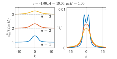
(a) Dressed energies (left) and distribution functions (right) for $n=1,2,3$

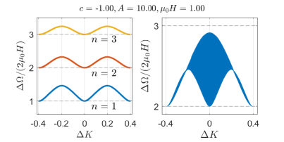
(b) Spectra of one $n$-string (left) and two length-$1$ strings (right)

Figure 12: (a) Dressed energies $\varepsilon_{n}^{0}\left(k\right)$ and distribution functions $\sigma_{n}^{0}\left(k\right)$ for $n=1,2,3$. The dressed energies $\varepsilon_{n}^{0}\left(k\right)$ tend to $2n\mu_{0}H$ for $k\rightarrow\pm\infty$. For the ground state, $\sigma_{n}^{0}$ give the distribution of holes because of $M_{n}=0$. (b) Excitation spectra of the spinon-bound-states . For a single length-$n$ string excitation, double degeneracy spectrum is observed (left). Right figure shows the continuum spectra of two length-$1$ spinons.

VI Conclusion and discussion

We have rigorously studied the excitation spectra of the Yang-Gaudin model with an attractive interaction. For the one particle-hole excitations in paired and unpaired fermions, the spectra apparently manifest a novel separation of collective motions of bosonic modes, i.e., the pairs-unpaired-fermions separation, which can be regarded as an evidence for the existence of the FFLO-state. We further analytically characterized this separation by calculating the curvature corrections to the linear dispersions of both paired and unpaired sections for a small momentum and a strong coupling regime. We have determined the sound velocities and effective masses in these dispersions, and compared with numerical results. We have showed that the free energy and the specific heat of the system can be simply expressed in a sum of inverse sound velocities of paired and unpaired Fermi seas at low temperatures, reflecting universal thermodynamics of TLLs. We have also studied other types of excitations, such as breaking or forming a pair and length-$n$ string excitations in the spin sector, in order to understand subtle novel pairing and deparing states. Here the gapped length-$n$ string excitations manifest a ferromagnetic coupling in the unpaired Fermi sea, i.e., magnon excitations.

Building on our results obtained, we expect to further study dynamical correlation functions for the charge-charge separation theory of FFLO states. According to the linear response theory kubo1957statistical , one can measure the spectra of pairing and depairing in the system by imposing a perturbation onto the system and observing their linear responses. The Bragg spectroscopy veeravalli2008bragg is one of a common experimental tools used to measure the many-body correlation. Using the Bragg spectroscopy, the recent experimentsenaratne2021spin did by Hulet’s group at Rice University have confirmed the spin-charge separation theory of TLLs in the 1D repulsive Fermi gas. In the Bragg spectroscopy, ${}^{6}Li$ atoms are trapped in 1D-tubes and two beams of different orientations are imposed onto the tubes. Due to the disturbance of the two beams, initially symmetrically distributed particles distribute asymmetrically in the tube. The dynamic structure factor (DSF) $S(q,\omega)$, usually defined as the density-density correlation, is related to the change of the total momentum as $\Delta P\propto[S(q,\omega)-S(-q,-\omega)]$. Therefore, the DSF is a measurable quantity in the experiment with both repulsive and attractive Fermi gases. Moreover, at low-energy excitations, the maximum (peak) of the DSF is related to the sound velocity, namely, the corresponding peak frequency is given by $\omega_{p}=v_{c}q$, and it is independent of the effective mass. Accordingly, different sound velocities of the paired and unpaired fermions can be observed by the Bragg spectroscopy, showing the subtle nature of the FFLO states in 1D.

Ackonwledgement

J.J.L. and X.W.G. are supported by the NSFC key grant No. 12134015, the NSFC grant No. 11874393 and No. 12121004. J.F.P. thanks the X.W.G.’s team members for helpful discussion and suggestion in completing his Master project and thank Innovation Academy for Precision Measurement Science and Technology, Chinese Academy of Sciences for kind hospitality.

Appendix

SM6.1 Express excited energies in dressed energies

First, introduce two useful formulas.

Formula 1: Any two groups of the analytical functions of the form

$$\begin{cases}\eta\left(k\right)=\eta^{0}\left(k\right)-\int_{-\lambda_{0}}^{\lambda_{0}}a_{1}\left(k-\lambda\right)\gamma\left(\lambda\right)\mathrm{d}\lambda\vspace{5pt}\\ \gamma\left(\lambda\right)=\gamma^{0}\left(\lambda\right)-\int_{-k_{0}}^{k_{0}}a_{1}\left(k-\lambda\right)\eta\left(k\right)\mathrm{d}k-\int_{-\lambda_{0}}^{\lambda_{0}}a_{2}\left(\lambda-\lambda^{\prime}\right)\gamma\left(\lambda^{\prime}\right)\mathrm{d}\lambda^{\prime}\end{cases}\vspace{5pt}$$ (A1)

$$\begin{cases}f\left(k\right)=f_{0}\left(k\right)-\int_{-\lambda_{0}}^{\lambda_{0}}a_{1}\left(k-\lambda\right)g\left(\lambda\right)\mathrm{d}\lambda\vspace{5pt}\\ g\left(\lambda\right)=g_{0}\left(\lambda\right)-\int_{-k_{0}}^{k_{0}}a_{1}\left(\lambda-k\right)f\left(k\right)\mathrm{d}k-\int_{-\lambda_{0}}^{\lambda_{0}}a_{2}\left(\lambda-\lambda^{\prime}\right)g\left(\lambda^{\prime}\right)\mathrm{d}\lambda^{\prime}\end{cases}$$

satisfy

$$\int_{-k_{0}}^{k_{0}}f_{0}\left(k\right)\eta\left(k\right)\mathrm{d}k+\int_{-\lambda_{0}}^{\lambda_{0}}g_{0}\left(\lambda\right)\gamma\left(\lambda\right)\mathrm{d}\lambda=\int_{-k_{0}}^{k_{0}}\eta^{0}\left(k\right)f\left(k\right)\mathrm{d}k+\int_{-\lambda_{0}}^{\lambda_{0}}\gamma^{0}\left(\lambda\right)g\left(\lambda\right)\mathrm{d}\lambda.$$ (A2)

One can prove it by multipy $\eta\left(k\right)$ and $f\left(k\right)$.

Formula 2: For any even analytical function $f\left(k\right)$ integrated between $\left[k_{-},k_{+}\right]$,where $k_{+}=k_{0}+\Delta Q_{+},k_{-}=$ $-k_{0}+\Delta Q_{-}$ (for $\Delta Q_{\pm}$ small enough), it can be expanded with $\Delta Q_{\pm}$, i.e.,

$$\int_{k_{-}}^{k_{+}}f\left(k\right)\mathrm{d}k=\int_{-k_{0}+\Delta Q_{-}}^{k_{0}+\Delta Q_{+}}f\left(k\right)\mathrm{d}k$$

$$= \int_{-k_{0}}^{k_{0}}f\left(k\right)\mathrm{d}k+\left[f\left(k_{0}\right)\Delta Q_{+}-f\left(-k_{0}\right)\Delta Q_{-}\right]+\mathcal{O}\left(\left(\Delta Q\right)^{2}\right),$$

so that

$$\int_{k_{-}}^{k_{+}}a_{n}\left(k-k^{\prime}\right)f\left(k^{\prime}\right)\mathrm{d}k^{\prime}$$

$$= \int_{-k_{0}}^{k_{0}}a_{n}\left(k-k^{\prime}\right)f\left(k^{\prime}\right)\mathrm{d}k+\left[a_{n}\left(k-k_{0}\right)\Delta Q_{+}-a_{n}\left(k+k_{0}\right)\Delta Q_{-}\right]f\left(k_{0}\right)+\mathcal{O}\left(\left(\Delta Q\right)^{2}\right)$$

If $k_{+}=-k_{-}=k_{0}+\Delta Q$, namely, $\Delta Q_{+}=-\Delta Q_{-}=\Delta Q$, the expansion can be expressed as

$$\int_{k-}^{k_{+}}f\left(k\right)\mathrm{d}k=\int_{-k_{0}-\Delta Q}^{k_{0}+\Delta Q}f\left(k\right)\mathrm{d}k=\int_{-k_{0}}^{k_{0}}f\left(k\right)\mathrm{d}k+2f\left(k_{0}\right)\Delta Q+\mathcal{O}\left(\left(\Delta Q\right)^{2}\right)$$

and

$$\int_{k_{-}}^{k_{+}}a_{n}\left(k-k^{\prime}\right)f\left(k^{\prime}\right)\mathrm{d}k^{\prime}$$

$$= \int_{-k_{0}}^{k_{0}}a_{n}\left(k-k^{\prime}\right)f\left(k^{\prime}\right)\mathrm{d}k^{\prime}+\left[a_{n}\left(k-k_{0}\right)+a_{n}\left(k+k_{0}\right)\right]f\left(k_{0}\right)\Delta Q+\mathcal{O}\left(\left(\Delta Q\right)^{2}\right).$$

Introducing $-\delta(k-k_{h})/L$ and $\delta(k-k_{p})/L$ into the distribution functions of unpaired fermions for one-particle hole excitations, we obtain

$$\bar{\sigma}\left(\lambda\right)= \frac{1}{\pi}-\int_{B_{-}}^{B_{+}}a_{2}\left(\lambda-k^{\prime}\right)\sigma\left(k^{\prime}\right)\mathrm{d}k^{\prime}-\int_{Q_{-}}^{Q_{+}}a_{1}\left(\lambda-k^{\prime}\right)\bar{\rho}\left(k^{\prime}\right)\mathrm{d}k^{\prime}$$ (A3)

$$+\frac{1}{L}a_{1}\left(\lambda-k_{h}\right)-\frac{1}{L}a_{1}\left(\lambda-k_{p}\right)$$

$$\bar{\rho}\left(k\right)= \frac{1}{2\pi}-\int_{B_{-}}^{B_{+}}a_{1}\left(k-k^{\prime}\right)\sigma\left(k^{\prime}\right)\mathrm{d}k^{\prime}.$$

According to Eq.(23), the excited energy density is given by

$$\frac{\Delta\Omega}{L}= \int_{Q_{-}}^{Q_{+}}\left[\bar{\rho}\left(k\right)-\frac{1}{L}\delta\left(k-k_{h}\right)+\frac{1}{L}\delta\left(k-k_{p}\right)\right]\left(k^{2}-\mu_{0}H\right)\mathrm{d}k-\int_{-Q_{0}}^{Q_{0}}\rho^{0}\left(k\right)\left(k^{2}-\mu_{0}H\right)\mathrm{d}k$$ (A4)

$$+2\int_{B_{-}}^{B_{+}}\sigma\left(\lambda\right)\left(\lambda^{2}-c^{2}\right)\mathrm{d}\lambda-2\int_{-B_{0}}^{B_{0}}\sigma\left(\lambda\right)\left(\lambda^{2}-c^{2}\right)\mathrm{d}\lambda$$

$$= \int_{-Q_{0}}^{Q_{0}}\Delta\bar{\rho}\left(k\right)\left(k^{2}-\mu_{0}H\right)\mathrm{d}k+2\bar{\rho}\left(Q_{0}\right)\left(Q_{0}^{2}-\mu_{0}H\right)\Delta Q-\frac{1}{L}k_{h}^{2}+\frac{1}{L}k_{p}^{2}$$

$$+2\int_{-B_{0}}^{B_{0}}\Delta\bar{\sigma}\left(\lambda\right)\left(\lambda^{2}-c^{2}\right)\mathrm{d}\lambda+4\bar{\sigma}\left(B_{0}\right)\left(B_{0}^{2}-c^{2}\right)\Delta B,$$

where $\Delta\bar{\rho}\left(k\right)=\bar{\rho}\left(k\right)-\rho^{0}\left(k\right)$, $\Delta\bar{\sigma}\left(\lambda\right)=\bar{\sigma}\left(\lambda\right)-\sigma^{0}\left(\lambda\right)$, and Formula.2 is used in the last step. Since the particle number does not change, i.e., $N-N_{G}=0$, we directly have

$$0= \int_{Q_{-}}^{Q_{+}}\rho\left(k\right)\mathrm{d}k-\int_{-Q_{0}}^{Q_{0}}\rho^{0}\left(k\right)\mathrm{d}k+2\int_{B_{-}}^{B_{+}}\sigma\left(\lambda\right)\mathrm{d}\lambda-2\int_{-B_{0}}^{B_{0}}\sigma^{0}\left(\lambda\right)\mathrm{d}\lambda$$ (A5)

$$= \int_{-Q_{0}}^{Q_{0}}\Delta\bar{\rho}\left(k\right)\mathrm{d}k+2\bar{\rho}\left(Q_{0}\right)\Delta Q-\frac{1}{L}+\frac{1}{L}+2\int_{-B_{0}}^{B_{0}}\Delta\bar{\sigma}\left(\lambda\right)\mathrm{d}\lambda+4\bar{\sigma}\left(B_{0}\right)\Delta B.$$

Substitute the last equation into the excited energy density, we obtain

$$\frac{\Delta\Omega}{L}= \int_{-Q_{0}}^{Q_{0}}\Delta\bar{\rho}\left(k\right)\left(k^{2}-A-\mu_{0}H\right)\mathrm{d}k+2\int_{-B_{0}}^{B_{0}}\Delta\bar{\sigma}\left(\lambda\right)\left(\lambda^{2}-A-c^{2}\right)\mathrm{d}\lambda$$ (A6)

$$+A\left[\frac{1}{L}-\frac{1}{L}-2\bar{\rho}\left(Q_{0}\right)\Delta Q-4\bar{\sigma}\left(B_{0}\right)\Delta\lambda\right]$$

$$+2\bar{\rho}\left(Q_{0}\right)\left(Q_{0}^{2}-\mu_{0}H\right)\Delta Q+4\bar{\sigma}\left(B_{0}\right)\left(B_{0}^{2}-c^{2}\right)\Delta B-\frac{1}{L}k_{h}^{2}+\frac{1}{L}k_{p}^{2}$$

$$= \int_{-Q_{0}}^{Q_{0}}\Delta\bar{\rho}\left(k\right)\left(k^{2}-A-\mu_{0}H\right)\mathrm{d}k+2\int_{-B_{0}}^{B_{0}}\Delta\bar{\sigma}\left(\lambda\right)\left(\lambda^{2}-A-c^{2}\right)\mathrm{d}\lambda$$

$$+2\left(Q_{0}^{2}-A-\mu_{0}H\right)\bar{\rho}\left(Q_{0}\right)\Delta Q+4\left(B_{0}^{2}-A-c^{2}\right)\bar{\sigma}\left(B_{0}\right)\Delta B$$

$$-\frac{1}{L}\left(k_{h}^{2}-A-\mu_{0}H\right)+\frac{1}{L}\left(k_{p}^{2}-A-\mu_{0}H\right).$$

According to Fomula.2, the change of distribution functions are given by

$$\Delta\bar{\sigma}\left(\lambda\right)= \bar{\sigma}\left(\lambda\right)-\sigma^{0}\left(\lambda\right)$$ (A7)

$$= -\int_{-Q_{0}}^{Q_{0}}a_{1}\left(\lambda-k\right)\Delta\bar{\rho}\left(k\right)\mathrm{d}k-\int_{-B_{0}}^{B_{0}}a_{2}\left(\lambda-\lambda^{\prime}\right)\Delta\bar{\sigma}\left(\lambda^{\prime}\right)\mathrm{d}\lambda$$

$$-\left[a_{1}\left(\lambda-Q_{0}\right)+a_{1}\left(\lambda+Q_{0}\right)\right]\bar{\rho}\left(Q_{0}\right)\Delta Q-\left[a_{2}\left(\lambda-B_{0}\right)+a_{2}\left(\lambda+B_{0}\right)\right]\bar{\sigma}\left(B_{0}\right)\Delta B$$

$$+\frac{1}{L}[a_{1}\left(\lambda-k_{h}\right)-a_{1}\left(\lambda-k_{p}\right)]$$

$$\Delta\bar{\rho}\left(k\right)= \bar{\rho}\left(k\right)-\rho^{0}\left(k\right)$$

$$= -\int_{-B_{0}}^{B_{0}}a_{1}\left(k-\lambda\right)\Delta\bar{\sigma}\left(\lambda\right)\mathrm{d}\lambda-\left[a_{1}\left(k-B_{0}\right)+a_{1}\left(k+B_{0}\right)\right]\bar{\sigma}\left(B_{0}\right)\Delta B.$$

While according to Fomula.1, we obtain the following relation,

$$2\int_{-B_{0}}^{B_{0}}\Delta\bar{\sigma}\left(\lambda\right)\left(k^{2}-A-c^{2}\right)\mathrm{d}\lambda+\int_{-Q_{0}}^{Q_{0}}\Delta\bar{\rho}\left(k\right)\left(k^{2}-A-\mu_{0}H\right)\mathrm{d}k$$ (A8)

$$= \int_{-B_{0}}^{B_{0}}\frac{1}{L}[a_{1}\left(\lambda-k_{h}\right)-a_{1}\left(\lambda-k_{p}\right)]\varepsilon^{0}\left(\lambda\right)\mathrm{d}\lambda$$

$$-\int_{-B_{0}}^{B_{0}}\left[a_{1}\left(\lambda-Q_{0}\right)+a_{1}\left(\lambda+Q_{0}\right)\right]\varepsilon^{0}\left(\lambda\right)\mathrm{d}\lambda\bar{\rho}\left(Q_{0}\right)\Delta Q$$

$$-\int_{-B_{0}}^{B_{0}}\left[a_{2}\left(\lambda-B_{0}\right)+a_{2}\left(\lambda+B_{0}\right)\right]\varepsilon^{0}\left(\lambda\right)\mathrm{d}\lambda\bar{\sigma}\left(B_{0}\right)\Delta B$$

$$-\int_{-Q_{0}}^{Q_{0}}\left[a_{1}\left(k-B_{0}\right)+a_{1}\left(k+B_{0}\right)\right]\kappa^{0}\left(k\right)\mathrm{d}k\bar{\sigma}\left(B_{0}\right)\Delta B$$

Since $\varepsilon^{0}\left(B_{0}\right)=\varepsilon^{0}\left(-B_{0}\right)=0$ and $\kappa^{0}\left(Q_{0}\right)=\kappa^{0}\left(-Q_{0}\right)=0$, we directly obtain

$$0= \varepsilon^{0}\left(B_{0}\right)+\varepsilon^{0}\left(-B_{0}\right)= 4\left(B_{0}^{2}-A-c^{2}\right)-\int_{-B_{0}}^{B_{0}}\left[a_{2}\left(\lambda-B_{0}\right)+a_{2}\left(\lambda+B_{0}\right)\right]\varepsilon^{0}\left(\lambda\right)\mathrm{d}\lambda$$ (A9)

$$-\int_{-Q_{0}}^{Q_{0}}\left[a_{1}\left(k-B_{0}\right)+a_{1}\left(k+B_{0}\right)\right]\kappa^{0}\left(k\right)\mathrm{d}k$$

$$0= \kappa^{0}\left(Q_{0}\right)+\kappa^{0}\left(-Q_{0}\right)= 2\left(Q_{0}^{2}-A-\mu_{0}H\right)-\int_{-B_{0}}^{B_{0}}\left[a_{1}\left(\lambda-Q_{0}\right)+a_{1}\left(\lambda+Q_{0}\right)\right]\varepsilon^{0}\left(\lambda\right)\mathrm{d}\lambda$$

Therefore, the last three terms of R.H.S. of Eq.(A8) can be substituted by the above relation (A9), namely,

$$2\int_{-B_{0}}^{B_{0}}\Delta\bar{\sigma}\left(\lambda\right)\left(k^{2}-A-c^{2}\right)\mathrm{d}\lambda+\int_{-Q_{0}}^{Q_{0}}\Delta\bar{\rho}\left(k\right)\left(k^{2}-A-\mu_{0}H\right)\mathrm{d}k$$ (A10)

$$= \int_{-B_{0}}^{B_{0}}\frac{1}{L}a_{1}\left(\lambda-k_{h}\right)\varepsilon^{0}\left(\lambda\right)\mathrm{d}\lambda-\int_{-B_{0}}^{B_{0}}\frac{1}{L}a_{1}\left(\lambda-k_{p}\right)\varepsilon^{0}\left(\lambda\right)\mathrm{d}\lambda$$

$$-2\left(Q_{0}^{2}-A-\mu_{0}H\right)\bar{\rho}\left(Q_{0}\right)\Delta Q-4\left(B_{0}^{2}-A-c^{2}\right)\bar{\sigma}\left(B_{0}\right)\Delta B.$$

Substitute the last equation into the excited energy, it follows that

$$\Delta\Omega= \int_{-B_{0}}^{B_{0}}a_{1}\left(\lambda-k_{h}\right)\varepsilon^{0}\left(\lambda\right)\mathrm{d}\lambda-\int_{-B_{0}}^{B_{0}}a_{1}\left(\lambda-k_{p}\right)\varepsilon^{0}\left(\lambda\right)\mathrm{d}\lambda-\left(k_{h}^{2}-A-\mu_{0}H\right)+\left(k_{p}^{2}-A-\mu_{0}H\right)$$ (A11)

$$= \kappa^{0}\left(k_{p}\right)-\kappa^{0}\left(k_{h}\right).$$

Together with Eq.(25), the dispersion of one-particle-hole excitation of the unpaired fermions is obtained.

The dispersion of paired fermions can be acquired in the same way. In brief, we again introduce two $\delta$-functions $-\delta\left(\lambda-\lambda_{h}\right)+\delta\left(\lambda-\lambda_{p}\right)$ as $\Delta\bar{\sigma}(\lambda)$. Accordingly, the distirbution funcitons are

$$\bar{\sigma}\left(\lambda\right)= \frac{1}{\pi}-\int_{B_{-}}^{B_{+}}a_{2}\left(\lambda-k^{\prime}\right)\sigma\left(k^{\prime}\right)\mathrm{d}k^{\prime}-\int_{Q_{-}}^{Q_{+}}a_{1}\left(\lambda-k^{\prime}\right)\bar{\rho}\left(k^{\prime}\right)\mathrm{d}k^{\prime}+\frac{1}{L}a_{1}\left(\lambda-\lambda_{h}\right)-\frac{1}{L}a_{1}\left(\lambda-\lambda_{p}\right)$$ (A12)

$$\bar{\rho}\left(k\right)= \frac{1}{2\pi}-\int_{B_{-}}^{B_{+}}a_{1}\left(k-k^{\prime}\right)\sigma\left(k^{\prime}\right)\mathrm{d}k^{\prime}+\frac{1}{L}a_{1}\left(\lambda-\lambda_{h}\right)-\frac{1}{L}a_{1}\left(\lambda-\lambda_{p}\right).$$

According to Eq.(23), the excited energy density is given by

$$\frac{\Delta\Omega}{L}= \int_{-Q_{0}}^{Q_{0}}\Delta\bar{\rho}\left(k\right)\left(k^{2}-\mu_{0}H\right)\mathrm{d}k+2\bar{\rho}\left(Q_{0}\right)\left(Q_{0}^{2}-\mu_{0}H\right)\Delta Q$$ (A13)

$$+2\int_{-B_{0}}^{B_{0}}\Delta\bar{\sigma}\left(\lambda\right)\left(\lambda^{2}-c^{2}\right)\mathrm{d}\lambda+4\bar{\sigma}\left(B_{0}\right)\left(B_{0}^{2}-c^{2}\right)\Delta B-\frac{1}{L}\lambda_{h}^{2}+\frac{1}{L}\lambda_{p}^{2}.$$

Using the same technique as that for unpaired fermions, one can essentially acquire the excited exergy given by Eq.(26).

In general, we can have excitations of $2N_{b}$ particle-holes in the paired sector and $2N_{u}$ in the unpaired sector simultaneously. One can easily prove that the multiple particle-hole excitations are simply a summation of single-particle-hole excitations with $2N_{u}+2N_{b}$ $\delta$-functions introduced into the distribution functions, i.e. $\sum_{i=1}^{N_{b}}[-\delta\left(k-k_{h,i}\right)+\delta\left(k-k_{p,i}\right)]/L$ and $\sum_{j=1}^{N_{u}}[-\delta\left(k-\lambda_{h,j}\right)+\delta\left(k-\lambda_{p,j}\right)]/L$.

For solely breaking and forming pairs, since there is no excitation of length-$n$ strings, the dispersions are similar to the above ones. The difference is likely that the excited state might be degenerate in this case due to the change of particle numbers of each sector, as described by Eq.(55).

For excitations of one length-$l$ string, the distribution functions are given by Eq.(59). Since there is exactly one occupied string, $\sigma_{n}(k)=\delta\left(k-\lambda_{l}\right)/L$. Then the excited free energy density Eq.(60) can be rewritten as

$$\frac{\Delta\Omega}{L}= \int_{Q_{-}}^{Q_{+}}\bar{\rho}\left(k\right)\left(k^{2}-\mu_{0}H\right)\mathrm{d}k-\int_{-Q_{0}}^{Q_{0}}\rho^{0}\left(k\right)\left(k^{2}-\mu_{0}H\right)\mathrm{d}k$$ (A14)

$$+2\int_{B_{-}}^{B_{+}}\bar{\sigma}\left(\lambda\right)\left(\lambda^{2}-c^{2}\right)\mathrm{d}\lambda-2\int_{-B_{0}}^{B_{0}}\sigma^{0}\left(\lambda\right)\left(\lambda^{2}-c^{2}\right)\mathrm{d}\lambda+\frac{2l\mu_{0}H}{L}\int_{B_{l+}}^{B_{l-}}\delta\left(k-\lambda_{l}\right)\mathrm{d}k$$

$$= \int_{-Q_{0}}^{Q_{0}}\Delta\bar{\rho}\left(k\right)\left(k^{2}-A-\mu_{0}H\right)\mathrm{d}k+2{\rho}\left(Q_{0}\right)\left(Q_{0}^{2}-A-\mu_{0}H\right)\Delta Q$$

$$+2\int_{-B_{0}}^{B_{0}}\Delta\bar{\sigma}\left(\lambda\right)\left(\lambda^{2}-A-c^{2}\right)\mathrm{d}\lambda+4\sigma\left(B_{0}\right)\left(B_{0}^{2}-A-c^{2}\right)\Delta B+\frac{2l\mu_{0}H}{L}.$$

Since the particle number is fixed, i.e., $N-N_{G}=0$, we directly obtain

$$\frac{\Delta\Omega}{L}= \int_{-Q_{0}}^{Q_{0}}\Delta\bar{\rho}\left(k\right)\left(k^{2}-A-\mu_{0}H\right)\mathrm{d}k+2\int_{-B_{0}}^{B_{0}}\Delta\bar{\sigma}\left(\lambda\right)\left(\lambda^{2}-A-c^{2}\right)\mathrm{d}\lambda$$ (A15)

$$+2\left(Q_{0}^{2}-A-\mu_{0}H\right)\rho\left(Q_{0}\right)\Delta Q+4\left(B_{0}^{2}-A-c^{2}\right)\sigma\left(B_{0}\right)\Delta B+\frac{2l\mu_{0}H}{L}.$$

According to Fomula.2, the changes of distribution functions are

$$\Delta\bar{\sigma}\left(\lambda\right)= \bar{\sigma}\left(\lambda\right)-\sigma^{0}\left(\lambda\right)=-\int_{-Q_{0}}^{Q_{0}}a_{1}\left(\lambda-k\right)\Delta\bar{\rho}\left(k\right)\mathrm{d}k-\left[a_{1}\left(\lambda-Q_{0}\right)+a_{1}\left(\lambda+Q_{0}\right)\right]{\rho}\left(Q_{0}\right)\Delta Q$$ (A16)

$$-\int_{-B_{0}}^{B_{0}}a_{2}\left(\lambda-\lambda^{\prime}\right)\Delta\bar{\sigma}\left(\lambda^{\prime}\right)\mathrm{d}\lambda-\left[a_{2}\left(\lambda-B_{0}\right)+a_{2}\left(\lambda+B_{0}\right)\right]\sigma\left(B_{0}\right)\Delta B$$

$$\Delta\bar{\rho}\left(k\right)= \bar{\rho}\left(k\right)-\rho^{0}\left(k\right)=-\int_{-B_{0}}^{B_{0}}a_{1}\left(k-\lambda\right)\Delta\bar{\sigma}\left(\lambda\right)\mathrm{d}\lambda-\left[a_{1}\left(k-B_{0}\right)+a_{1}\left(k+B_{0}\right)\right]\sigma\left(B_{0}\right)\Delta B.$$

According to Fomula.1 and the expression of derssed energies, we have

$$2\int_{-B_{0}}^{B_{0}}\Delta\bar{\sigma}\left(\lambda\right)\left(k^{2}-A-c^{2}\right)\mathrm{d}\lambda+\int_{-Q_{0}}^{Q_{0}}\Delta\bar{\rho}\left(k\right)\left(k^{2}-A-\mu_{0}H\right)\mathrm{d}k$$ (A17)

$$= -\int_{-B_{0}}^{B_{0}}\left[a_{1}\left(\lambda-Q_{0}\right)+a_{1}\left(\lambda+Q_{0}\right)\right]\varepsilon^{0}\left(\lambda\right)\mathrm{d}\lambda{\rho}\left(Q_{0}\right)\Delta Q$$

$$-\int_{-B_{0}}^{B_{0}}\left[a_{2}\left(\lambda-B_{0}\right)+a_{2}\left(\lambda+B_{0}\right)\right]\varepsilon^{0}\left(\lambda\right)\mathrm{d}\lambda\sigma\left(B_{0}\right)\Delta B$$

$$-\int_{-Q_{0}}^{Q_{0}}\left[a_{1}\left(k-B_{0}\right)+a_{1}\left(k+B_{0}\right)\right]\kappa^{0}\left(k\right)\mathrm{d}k\sigma\left(B_{0}\right)\Delta B-\int_{-Q_{0}}^{Q_{0}}\frac{1}{L}a_{l}\left(k-\lambda\right)\kappa^{0}\left(k\right)\mathrm{d}k.$$

Since $\varepsilon^{0}\left(B_{0}\right)+\varepsilon^{0}\left(-B_{0}\right)=0$ and $\kappa^{0}\left(Q_{0}\right)+\kappa^{0}\left(-Q_{0}\right)=0$, the frist three terms of R.H.S. of the last equatoin can be rewritten. Namely, we have

$$2\int_{-B_{0}}^{B_{0}}\Delta\bar{\sigma}\left(\lambda\right)\left(k^{2}-A-c^{2}\right)\mathrm{d}\lambda+\int_{-Q_{0}}^{Q_{0}}\Delta\bar{\rho}\left(k\right)\left(k^{2}-A-\mu_{0}H\right)\mathrm{d}k$$ (A18)

$$= -\int_{-Q_{0}}^{Q_{0}}\frac{1}{L}a_{l}\left(k-\lambda\right)\kappa^{0}\left(k\right)\mathrm{d}k.-2\left(Q_{0}^{2}-A-\mu_{0}H\right){\rho}\left(Q_{0}\right)\Delta Q-4\left(B_{0}^{2}-A-c^{2}\right)\sigma\left(B_{0}\right)\Delta B$$

Substituting the last equation into Eq.(A15) we obtain the excited energy Eq.(61) expressed in the length-$\ell$-string dressed energy.

SM6.2 Sound Velocity and Effective Mass from Bethe Ansatz

In Section III.2, we derived sound velocities and effective masses of paired and unpaired fermions from the zero-temperature TBA equations. Here we apply the method of Ref.he2020emergence to derive the results from the BA equations in detail.

Since $M_{n}=0$ at the ground state, the logarithm of the BA equations of the two charge sectors are

$$2\Lambda_{\alpha}L=2\pi J_{\alpha}+\sum_{j=1}^{N-2M}\theta\left(\frac{\Lambda_{\alpha}-k_{j}}{|c|}\right)+\sum_{\beta=1}^{M}\theta\left(\frac{\Lambda_{\alpha}-\Lambda_{\beta}}{2|c|}\right), \alpha=1,2,\cdots,M$$ (A19)

$$k_{j}L=2\pi I_{j}+\sum_{\alpha=1}^{M}\theta\left(\frac{k_{j}-\Lambda_{\alpha}}{|c|}\right), j=1,\cdots,N-2M$$

For the ground state, at the thermodynamic limit, we can expand both equations with coupling strength up to order $\sim\mathcal{O}(1/c)$, the first of which gives

$$\Lambda_{\alpha}\approx \frac{\pi}{L}J_{\alpha}+\frac{1}{2L}\sum_{j=1}^{N-2M}2\left[\arctan\left(\frac{-k_{j}}{\left|c\right|}\right)+\frac{1}{1+\left(k_{j}/c\right)^{2}}\frac{\Lambda_{\alpha}}{\left|c\right|}\right]$$

$$+\frac{1}{2L}\sum_{\beta=1}^{M}2\left[\arctan\left(\frac{-\Lambda_{\beta}}{2\left|c\right|}\right)+\frac{1}{1+\left(\Lambda_{\beta}/c\right)^{2}/4}\frac{\Lambda_{\alpha}}{2\left|c\right|}\right].$$

If $k_{j}$ and $\Lambda_{\beta}$ are both symmetrically distributed to the zero-point, the $\arctan$-terms drop out in the sum with respect to $j$ and $\beta$. Namely, we have

$$\Lambda_{\alpha}=\frac{\pi}{L}J_{\alpha} +\frac{1}{L}\sum_{j=1}^{N-2M}\frac{1}{1+\left(k_{j}/c\right)^{2}}\frac{\Lambda_{\alpha}}{\left|c\right|}+\frac{1}{L}\sum_{\beta=1}^{M}\frac{1}{1+\left(\Lambda_{\beta}/c\right)^{2}/4}\frac{\Lambda_{\alpha}}{2\left|c\right|}$$ (A20)

$$=\frac{\pi}{L}J_{\alpha} +\int_{-Q}^{Q}\frac{1}{1+\left(k_{j}/c\right)^{2}}\rho\left(k\right)\mathrm{d}k\frac{\Lambda_{\alpha}}{\left|c\right|}+\int_{-B}^{B}\frac{1}{1+\left(\lambda/c\right)^{2}/4}\sigma\left(\lambda\right)\mathrm{d}\lambda\frac{\Lambda_{\alpha}}{2\left|c\right|}$$

$$=\frac{\pi}{L}J_{\alpha} +\int_{-Q}^{Q}\frac{1}{1+\left(k_{j}/c\right)^{2}}\left[\frac{1}{2\pi}-a_{1}\left(k\right)n_{b}\right]\mathrm{d}k\frac{\Lambda_{\alpha}}{\left|c\right|}$$

$$+\int_{-B}^{B}\frac{1}{1+\left(\lambda/c\right)^{2}/4}\left[\frac{1}{\pi}-a_{2}\left(\lambda\right)n_{b}-a_{1}\left(\lambda\right)n_{u}\right]\mathrm{d}\lambda\frac{\Lambda_{\alpha}}{2\left|c\right|}$$

$$\approx\frac{\pi}{L}J_{\alpha} +\left[\frac{\left|c\right|}{\pi}\arctan\left(\frac{Q}{\left|c\right|}\right)+\frac{2\left|c\right|}{\pi}\arctan\left(\frac{B}{2\left|c\right|}\right)\right]\frac{\Lambda_{\alpha}}{\left|c\right|}$$

$$\approx\frac{\pi}{L}J_{\alpha} +\frac{Q+B}{\pi\left|c\right|}\Lambda_{\alpha};$$

if $k_{j}$ or $\Lambda_{\beta}$ is asymmetrically distributed to the zero-point, there is an additional but negligible term

$$\pm\frac{1}{L}\arctan(\frac{\pi n_{u}}{\left|c\right|})\approx\pm\frac{\pi n_{u}}{L\left|c\right|}\ll\frac{\pi}{L}J_{\alpha}\quad\text{or}\quad\pm\frac{1}{L}\arctan(\frac{\pi n_{b}}{\left|c\right|})\approx\pm\frac{\pi n_{b}}{L\left|c\right|}\ll\frac{\pi}{L}J_{\alpha},$$ (A21)

respectively. According to Eq.(A20) and (A21), the approximation of $\Lambda_{\alpha}$ is independent of the parity of $k_{j}$. By substituting Eq.(39) into Eq.(A20), we have

$$\Lambda_{\alpha}=\left(1-\frac{Q+B}{\pi\left|c\right|}\right)^{-1}\frac{\pi}{L}J_{\alpha}\approx\left(1+\frac{Q+B}{\pi\left|c\right|}\right)\frac{\pi}{L}J_{\alpha}\approx\left(1+\frac{1}{2\gamma_{b}}+\frac{1}{\gamma_{u}}\right)\frac{\pi}{L}J_{\alpha},$$ (A22)

where the first term of RHS of the last equation $\pi J_{\alpha}/L$ equals the quasimomentum of free paired fermions, while the remaining terms emerge from the interactions among fermions.

The total energy and momentum of the paired fermions are given by

$$E_{b}=2\sum_{\alpha=1}^{M}\Lambda_{\alpha}^{2}=2\left(1+\tau_{b}\right)^{2}\left(\frac{\pi}{L}\right)^{2}\sum_{\alpha=1}^{M}J_{\alpha}^{2},\quad K_{b}=2\sum_{\alpha=1}^{M}\Lambda_{\alpha}=2\left(1+\tau_{b}\right)\frac{\pi}{L}\sum_{\alpha=1}^{M}J_{\alpha}.$$ (A23)

where $\tau_{b}=\frac{1}{2\gamma_{b}}+\frac{1}{\gamma_{u}}$. For one-particle-hole excitation near the Fermi surface, the quantum number of the excited particle and hole are

$$\left|J_{p}\right|>\frac{M-1}{2},\quad\left|J_{h}\right|=\frac{M-1}{2}-\beta<\frac{M-1}{2},\text{ }\beta\in\mathbb{Z}^{+}\text{ and }\beta\ll M,$$ (A24)

where $\beta$ is chosen to be much smaller than $M$ so that the excitation is taken near the Fermi surface. Therefore, the excited momentum of free paired fermions is

$$\Delta K_{b,0}=2\frac{\pi}{L}\left(J_{p}-J_{h}\right);$$ (A25)

whereas the excited energy of attractive paired fermions is

$$\Delta E_{b} =2\left(1+\tau_{b}\right)^{2}\left(\frac{\pi}{L}\right)^{2}\left(J_{p}^{2}-J_{h}^{2}\right)=2\left(1+\tau_{b}\right)^{2}\left(\frac{\pi}{L}\right)^{2}\frac{L\Delta K_{b,0}}{2\pi}\left[\left(M-1-2\beta\right)+\frac{L\Delta K_{b,0}}{2\pi}\right]$$ (A26)

$$=\left(1+\tau_{b}\right)^{2}\pi n_{b}\Delta K_{b,0}+\frac{\left(1+\tau_{b}\right)^{2}}{2}\left(\Delta K_{b,0}\right)^{2}+\mathcal{O}\left(\frac{1}{L}\right).$$

We would like to express this dispersion in free-fermion approximation, with the mass of free fermion $m$ (set to be $1/2$ previously) replaced by the effective mass $m^{*}$ due to the interactions. Namely,

$$\Delta E_{b}=2\left[v_{b}\frac{\Delta K_{b,0}}{2}+\frac{1}{2m_{b}^{*}}\left(\frac{\Delta K_{b,0}}{2}\right)^{2}\right],$$ (A27)

By comparison of Eq,(A26) and (A27), the sound velocities and effective masses are given by

$$v_{b}=\pi n_{b}\left(1+\frac{1}{2\gamma_{b}}+\frac{1}{\gamma_{u}}\right)^{2}\approx\pi n_{b}\left(1+\frac{1}{\gamma_{b}}+\frac{2}{\gamma_{u}}\right),$$ (A28)

$$m^{*}_{b}=m\left(1+\frac{1}{2\gamma_{b}}+\frac{1}{\gamma_{u}}\right)^{-2}\approx m\left(1-\frac{1}{\gamma_{b}}-\frac{2}{\gamma_{u}}\right),$$

which is the same as the sound velocity and effective mass of paired fermions in Eq.(45).

Similarly, we can calculate these quantities of unpaired sectors. By expanding the second equation of Eq.(A19), we have

$$k_{j}\approx\frac{2\pi}{L}I_{j}+\frac{4B}{\pi\left|c\right|}k_{j}\approx\left(1+\frac{4B}{\pi\left|c\right|}\right)\frac{2\pi}{L}I_{j}\approx\left(1+\frac{2}{\gamma_{b}}\right)\frac{2\pi}{L}I_{j}.$$ (A29)

The dispersion of unpaired fermions can be expressed as

$$\Delta E_{u} =\left(1-\tau_{u}\right)^{2}2\pi n_{u}\Delta K_{u,0}+\left(1-\tau_{u}\right)^{2}\left(\Delta K_{u,0}\right)^{2}+\mathcal{O}\left(\frac{1}{L}\right)$$ (A30)

$$=v_{u}\Delta K_{u,0}+\frac{1}{2m^{*}_{u}}\left(\Delta K_{u,0}\right)^{2}.$$

Therefore, the sound velocity and effective mass of unpaired fermions are

$$v_{u}=2\pi n_{u}\left(1+\frac{2}{\gamma_{b}}\right)^{2}\approx 2\pi n_{u}\left(1+\frac{4}{\gamma_{b}}\right),$$ (A31)

$$m^{*}_{u}=m\left(1+\frac{2}{\gamma_{b}}\right)^{-2}\approx m\left(1-\frac{4}{\gamma_{b}}\right),$$

which is the same as the sound velocity and effective mass of unpaired fermions in Eqs. (47).

SM6.3 Free Energy at Low Temperature

To distinguish quantities at zero-temperature and low-temperature, we introduce the subscript "0" indicating zero-temperature. Accordingly, dressed energies at zero-temperature $\varepsilon_{0}$ and $\kappa_{0}$ given by Eq.(15); while dressed energies at low-temperature can be expanded with respect to zero-temperature as $\varepsilon=\varepsilon_{0}+\beta$ and $\kappa=\kappa_{0}+\gamma$. Namely, we have

$$\varepsilon(k)= 2(k^{2}-A-c^{2})+T\int a_{2}(k-k^{\prime})\ln{(1+e^{-\frac{\varepsilon(k^{\prime})}{T}})}\mathrm{d}k^{\prime}+T\int a_{1}(k-k^{\prime})\ln{(1+e^{-\frac{\kappa(k^{\prime})}{T}})}\mathrm{d}k^{\prime}$$ (A32)

$$\approx 2(k^{2}-A-c^{2})+T\int a_{2}(k-k^{\prime})\ln{(1+e^{-\frac{\left|\varepsilon(k^{\prime})\right|}{T}})}\mathrm{d}k^{\prime}-\int_{-B}^{B}a_{2}(k-k^{\prime})\varepsilon(k^{\prime})\mathrm{d}k^{\prime}$$

$$+T\int a_{1}(k-k^{\prime})\ln{(1+e^{-\frac{\left|\kappa(k^{\prime})\right|}{T}})}\mathrm{d}k^{\prime}-\int_{-Q}^{Q}a_{1}(k-k^{\prime})\kappa(k^{\prime})\mathrm{d}k^{\prime}$$

$$= \varepsilon_{0}(k)+T\int a_{2}(k-k^{\prime})\ln{(1+e^{-\frac{\left|\varepsilon(k^{\prime})\right|}{T}})}\mathrm{d}k^{\prime}-\int_{-B}^{B}a_{2}(k-k^{\prime})\beta(k^{\prime})\mathrm{d}k^{\prime}$$

$$+T\int a_{1}(k-k^{\prime})\ln{(1+e^{-\frac{\left|\kappa(k^{\prime})\right|}{T}})}\mathrm{d}k^{\prime}-\int_{-Q}^{Q}a_{1}(k-k^{\prime})\gamma(k^{\prime})\mathrm{d}k^{\prime},$$

$$\kappa(k)= k^{2}-A-\mu_{0}H+T\int a_{1}(k-k^{\prime})\ln{(1+e^{-\frac{\varepsilon(k^{\prime})}{T}})}\mathrm{d}k^{\prime}$$

$$\approx k^{2}-A-\mu_{0}H+T\int a_{1}(k-k^{\prime})\ln{(1+e^{-\frac{\left|\varepsilon(k^{\prime})\right|}{T}})}\mathrm{d}k^{\prime}-\int_{-B}^{B}a_{1}(k-k^{\prime})\varepsilon(k^{\prime})\mathrm{d}k^{\prime}$$

$$= \kappa_{0}(k)+T\int a_{1}(k-k^{\prime})\ln{(1+e^{-\frac{\left|\varepsilon(k^{\prime})\right|}{T}})}\mathrm{d}k^{\prime}-\int_{-B}^{B}a_{1}(k-k^{\prime})\beta(k^{\prime})\mathrm{d}k^{\prime},$$

where we omitted the integral intervals $(-\infty,\infty)$ for convenience of notation. Since for low-temperature, the integrals on the R.H.S. of the last two equations mostly attribute to the values of integrands near the Fermi momenta $B$ and $Q$, we replace $\varepsilon(k)$ and $\kappa(k)$ with their linear expansions $(k-B)u_{b}$ and $(k-Q)u_{u}$, respectively, where $u_{b}$ and $u_{u}$ denote $\varepsilon^{\prime}(B)$ and $\kappa^{\prime}(Q)$, respectively. Namely, we have

$$\varepsilon(k)=\varepsilon_{0}+\beta= \varepsilon_{0}(k)+\frac{\pi^{2}T^{2}}{6u_{b}}\left[a_{2}(k-B)+a_{2}(k+B)\right]-\int_{-B}^{B}a_{2}(k-k^{\prime})\beta(k^{\prime})\mathrm{d}k^{\prime}$$ (A33)

$$+\frac{\pi^{2}T^{2}}{6u_{u}}\left[a_{1}(k-Q)+a_{1}(k+Q)\right]-\int_{-Q}^{Q}a_{1}(k-k^{\prime})\gamma(k^{\prime})\mathrm{d}k^{\prime},$$

$$\kappa(k)=\kappa_{0}+\gamma= \kappa_{0}(k)+\frac{\pi^{2}T^{2}}{6u_{b}}\left[a_{1}(k-B)+a_{1}(k+B)\right]-\int_{-B}^{B}a_{1}(k-k^{\prime})\beta(k^{\prime})\mathrm{d}k^{\prime}.$$

We further denote $\beta_{0}(k)=(\pi^{2}T^{2})/(6u_{b})\left[a_{2}(k-B)+a_{2}(k+B)\right]+(\pi^{2}T^{2})/(6u_{u})\left[a_{1}(k-Q)+\right.$ $\left.a_{1}(k+Q)\right]$ and $\gamma_{0}(k)=(\pi^{2}T^{2})/(6u_{b})\left[a_{1}(k-B)+a_{1}(k+B)\right]$, so that the last equations can be simplified as

$$\varepsilon(k)=\varepsilon_{0}+\beta= \varepsilon_{0}+\beta_{0}-\int_{-B}^{B}a_{2}(k-k^{\prime})\beta(k^{\prime})\mathrm{d}k^{\prime}-\int_{-Q}^{Q}a_{1}(k-k^{\prime})\gamma(k^{\prime})\mathrm{d}k^{\prime},$$ (A34)

$$\kappa(k)=\kappa_{0}+\gamma= \kappa_{0}+\gamma_{0}-\int_{-B}^{B}a_{1}(k-k^{\prime})\beta(k^{\prime})\mathrm{d}k^{\prime}.$$

According to Eq.(13), the free energy density (i.e., pressure) at zero-temperature is given by

$$\Omega_{0}/L=p_{0}=-\frac{1}{\pi}\int_{-B}^{B}\varepsilon_{0}(k)\mathrm{d}k-\frac{1}{2\pi}\int_{-Q}^{Q}\kappa_{0}(k)\mathrm{d}k;$$ (A35)

while the free energy density at low temperature can be expanded with respect to zero-temperature by

$$\Omega/L=p$$ (A36)

$$= -\frac{1}{\pi}\int_{-B}^{B}\varepsilon(k)\mathrm{d}k-\frac{1}{2\pi}\int_{-Q}^{Q}\kappa(k)\mathrm{d}k+T\int\ln{(1+e^{-\frac{\left|\varepsilon(k^{\prime})\right|}{T}})}\frac{\mathrm{d}k}{\pi}+T\int\ln{(1+e^{-\frac{\left|\kappa(k^{\prime})\right|}{T}})}\frac{\mathrm{d}k}{2\pi}$$

$$= p_{0}-\frac{1}{\pi}\int_{-B}^{B}\beta(k)\mathrm{d}k-\frac{1}{2\pi}\int_{-Q}^{Q}\gamma(k)\mathrm{d}k+\frac{\pi T^{2}}{3u_{b}}+\frac{\pi T^{2}}{6u_{u}}.$$

Below we will prove that the last four terms on the R.H.S can be expressed in sound velocities $v_{b}$ and $v_{u}$.

First, we calculate $\int_{-Q}^{Q}\gamma(k)\rho(k)\mathrm{d}k$. According to expressions of distribution functions given by Eq.(17) and $\beta(k)$ and $\gamma(k)$ given by Eq.(A34), we have

$$\frac{1}{2\pi}\int_{-Q}^{Q}\gamma(k)\mathrm{d}k-\int_{-Q}^{Q}\int_{-B}^{B}a_{1}(k-k^{\prime})\sigma(k^{\prime})\gamma(k)\mathrm{d}k^{\prime}\mathrm{d}k$$ (A37)

$$= \int_{-Q}^{Q}\rho(k)\gamma_{0}(k)\mathrm{d}k+\int_{-Q}^{Q}\int_{-B}^{B}\rho(k)a_{1}(k^{\prime}-k)\beta(k^{\prime})\mathrm{d}k^{\prime}\mathrm{d}k$$

$$= \int_{-Q}^{Q}\rho(k)\gamma_{0}(k)\mathrm{d}k+\int_{-B}^{B}\left[\sigma(k^{\prime})-\frac{1}{\pi}+\int_{-B}^{B}a_{2}(k-k^{\prime})\sigma(k^{\prime})\mathrm{d}k\right]\beta(k^{\prime})\mathrm{d}k^{\prime}$$

$$= \int_{-Q}^{Q}\rho(k)\gamma_{0}(k)\mathrm{d}k+\left(\int_{-B}^{B}\sigma(k^{\prime})\beta_{0}(k^{\prime})\mathrm{d}k^{\prime}-\int_{-B}^{B}\int_{-B}^{B}\sigma(k^{\prime})a_{2}(k^{\prime}-k)\beta(k)\mathrm{d}k\mathrm{d}k^{\prime}\right.$$

$$\left.-\int_{-B}^{B}\int_{-Q}^{Q}\sigma(k^{\prime})a_{1}(k^{\prime}-k)\gamma(k)\mathrm{d}k\mathrm{d}k^{\prime}\right)-\frac{1}{\pi}\int_{-B}^{B}\beta(k^{\prime})\mathrm{d}k^{\prime}+\int_{-B}^{B}\int_{-B}^{B}a_{2}(k-k^{\prime})\sigma(k^{\prime})\beta(k^{\prime})\mathrm{d}k\mathrm{d}k^{\prime},$$

where the last term on the L.H.S should cancel with the fourth term on the R.H.S, and the third and last terms on the R.H.S should cancel with each other. By rearranging the last equation and substituting $\beta_{0}$ and $\gamma_{0}$ into it, we have

$$\frac{1}{\pi}\int_{-B}^{B}\beta(k)\mathrm{d}k+\frac{1}{2\pi}\int_{-Q}^{Q}\gamma(k)\mathrm{d}k=\int_{-B}^{B}\sigma(k)\beta_{0}(k)\mathrm{d}k+\int_{-Q}^{Q}\rho(k)\gamma_{0}(k)\mathrm{d}k$$ (A38)

$$= \frac{\pi^{2}T^{2}}{6u_{b}}\int_{-B}^{B}\sigma(k)\left[a_{2}(k-B)+a_{2}(k+B)\right]\mathrm{d}k+\frac{\pi^{2}T^{2}}{6u_{u}}\int_{-B}^{B}\sigma(k)\left[a_{1}(k-Q)+a_{1}(k+Q)\right]\mathrm{d}k$$

$$+\frac{\pi^{2}T^{2}}{6u_{b}}\int_{-Q}^{Q}\rho(k)\left[a_{1}(k-B)+a_{1}(k+B)\right]\mathrm{d}k$$

$$= \frac{\pi^{2}T^{2}}{6u_{b}}\left[\frac{2}{\pi}-2\sigma(B)\right]+\frac{\pi^{2}T^{2}}{6u_{u}}\left[\frac{1}{\pi}-2\rho(Q)\right],$$

where the last step is because that since $a_{n}(k)$ is even, we have $2\sigma(B)=2/\pi-\int_{-B}^{B}\left[a_{2}(k-B)+\right.$ $\left.a_{2}(k+B)\right]\sigma(k)\mathrm{d}k-\int_{-Q}^{Q}\left[a_{1}(k-B)+a_{1}(k+B)\right]\rho(k)\mathrm{d}k$ and $2\rho(Q)=1/\pi-\int_{-B}^{B}\left[a_{1}(k-Q)+\right.$ $\left.a_{1}(k+Q)\right]\sigma(k)\mathrm{d}k$. By substituting Eq.(A38) into Eq.(A36), the free energy density can be written as

$$\Omega/L-\Omega_{0}/L=p-p_{0}= -\frac{\pi T^{2}}{3u_{b}}+\frac{\pi^{2}T^{2}\sigma(B)}{3u_{b}}-\frac{\pi T^{2}}{6u_{u}}+\frac{\pi^{2}T^{2}\rho(Q)}{3u_{u}}+\frac{\pi T^{2}}{3u_{b}}+\frac{\pi T^{2}}{6u_{u}}$$ (A39)

$$= \frac{\pi T^{2}}{6}\left(\frac{1}{v_{b}}+\frac{1}{v_{u}}\right),$$

where we used the relation between sound velocities and distribution functions and dressed energies given by Eqs.(33) and (36), which is the same as Eq.(50).

References

- (1) Gordon Baym and Christopher Pethick. Landau Fermi-liquid theory: concepts and applications. John Wiley & Sons, 2008.
- (2) LD Landau. Oscillations in a fermi liquid. Sov. Phys. JETP, 5(1):101–108, 1957.
- (3) LD Landau. Fermi liquid theory. Sov. Phys. JETP, 3:920–929, 1956.
- (4) Sin-itiro Tomonaga. Remarks on bloch’s method of sound waves applied to many-fermion problems. Progress of Theoretical Physics, 5(4):544–569, 1950.
- (5) JM Luttinger. An exactly soluble model of a many-fermion system. Journal of mathematical physics, 4(9):1154–1162, 1963.
- (6) Daniel C Mattis and Elliott H Lieb. Exact solution of a many-fermion system and its associated boson field. In Bosonization, pages 98–106. World Scientific, 1994.
- (7) FDM Haldane. ’Luttinger liquid theory’of one-dimensional quantum fluids. i. properties of the luttinger model and their extension to the general 1d interacting spinless fermi gas. Journal of Physics C: Solid State Physics, 14(19):2585, 1981.
- (8) Thierry Giamarchi. Quantum physics in one dimension, (Oxford: Oxford University Press), 2004.
- (9) MA Cazalilla, Roberta Citro, Thierry Giamarchi, Edmond Orignac, and Marcos Rigol. One dimensional bosons: From condensed matter systems to ultracold gases. Reviews of Modern Physics, 83(4):1405, 2011.
- (10) Fabian HL Essler, Holger Frahm, Frank Göhmann, Andreas Klümper, and Vladimir E Korepin. The one-dimensional Hubbard model. Cambridge University Press, 2005.
- (11) Xi-Wen Guan, Murray T Batchelor, and Chaohong Lee. Fermi gases in one dimension: From bethe ansatz to experiments. Reviews of Modern Physics, 85(4):1633, 2013.
- (12) Hans Bethe. Zur theorie der metalle. Zeitschrift für Physik, 71(3):205–226, 1931.
- (13) Chen-Ning Yang and Chen-Ping Yang. One-dimensional chain of anisotropic spin-spin interactions. i. proof of bethe’s hypothesis for ground state in a finite system. Physical Review, 150(1):321, 1966.
- (14) Chen-Ning Yang and Chen-Ping Yang. One-dimensional chain of anisotropic spin-spin interactions. ii. properties of the ground-state energy per lattice site for an infinite system. Physical Review, 150(1):327, 1966.
- (15) Chen-Ning Yang and Chen-Ping Yang. One-dimensional chain of anisotropic spin-spin interactions. iii. applications. Physical Review, 151(1):258, 1966.
- (16) Elliott H Lieb and Werner Liniger. Exact analysis of an interacting bose gas. i. the general solution and the ground state. Physical Review, 130(4):1605, 1963.
- (17) James B McGuire. Study of exactly soluble one-dimensional n-body problems. Journal of Mathematical Physics, 5(5):622–636, 1964.
- (18) Chen-Ning Yang. Some exact results for the many-body problem in one dimension with repulsive delta-function interaction. Physical Review Letters, 19(23):1312, 1967.
- (19) Chen N Yang. S matrix for the one-dimensional n-body problem with repulsive or attractive -function interaction. Physical Review, 168(5):1920, 1968.
- (20) M Gaudin. Un systeme a une dimension de fermions en interaction. Physics Letters A, 24(1):55–56, 1967.
- (21) Rodney J Baxter. Partition function of the eight-vertex lattice model. Annals of Physics, 70(1):193–228, 1972.
- (22) Chen-Ning Yang and Cheng P Yang. Thermodynamics of a one-dimensional system of bosons with repulsive delta-function interaction. Journal of Mathematical Physics, 10(7):1115–1122, 1969.
- (23) Minoru Takahashi. Thermodynamics of one-dimensional solvable models. Thermodynamics of One-Dimensional Solvable Models, (Cambridge: Cambridge University Press) 2005.
- (24) Minoru Takahashi. Ground state energy of the one-dimensional electron system with short-range interaction. i. Progress of Theoretical Physics, 44(2):348–358, 1970.
- (25) Minoru Takahashi. Many-body problem of attractive fermions with arbitrary spin in one dimension. Progress of Theoretical Physics, 44(4):899–904, 1970.
- (26) Minoru Takahashi. One-dimensional electron gas with delta-function interaction at finite temperature. In Exactly Solvable Models Of Strongly Correlated Electrons, pages 388–406. World Scientific, 1994.
- (27) Minoru Takahashi et al. Magnetic susceptibility for the half-filled hubbard model. Prog. Theor. Phys, 43(6), 1970.
- (28) Xi-Wen Guan and Feng He. Professor chen ping yang’s early significant contributions to mathematical physics. International Journal of Modern Physics B, 33(06):1930002,2019.
- (29) X.-W. Guan and P. He, in press (2022).
- (30) Peter Fulde and Richard A Ferrell. Superconductivity in a strong spin-exchange field. Physical Review, 135(3A):A550, 1964.
- (31) AI Larkin and Yu N Ovchinnikov. Zh. é ksp. teor. fiz. 47, 1136 1964 sov. phys. JETP, 20:762, 1965.
- (32) X.-W. Guan and H.-Q. Lin, in press (2022).
- (33) Xi-Wen Guan, MT Batchelor, C Lee, and M Bortz. Phase transitions and pairing signature in strongly attractive fermi atomic gases. Physical Review B, 76(8):085120, 2007.
- (34) G Orso. Attractive fermi gases with unequal spin populations in highly elongated traps. Physical review letters, 98(7):070402, 2007.
- (35) Hui Hu, Xia-Ji Liu, and Peter D Drummond. Phase diagram of a strongly interacting polarized fermi gas in one dimension. Physical review letters, 98(7):070403, 2007.
- (36) Yean-an Liao, Ann Sophie C Rittner, Tobias Paprotta, Wenhui Li, Guthrie B Partridge, Randall G Hulet, Stefan K Baur, and Erich J Mueller. Spin-imbalance in a one-dimensional fermi gas. Nature, 467(7315):567–569, 2010.
- (37) Xi-wen Guan and Tin-Lun Ho. Quantum criticality of a one-dimensional attractive fermi gas. Physical Review A, 84(2):023616, 2011.
- (38) Li Peng, Yicong Yu, and Xi-Wen Guan. Grüneisen parameters for the lieb-liniger and yang-gaudin models. Physical Review B, 100(24):245435, 2019.
- (39) X-W Guan, X-G Yin, Angela Foerster, Murray T Batchelor, C-H Lee, and H-Q Lin. Wilson ratio of fermi gases in one dimension. Physical review letters, 111(13):130401, 2013.
- (40) Yi-Cong Yu, Yang-Yang Chen, Hai-Qing Lin, Rudolf A Römer, and Xi-Wen Guan. Dimensionless ratios: Characteristics of quantum liquids and their phase transitions. Physical Review B, 94(19):195129, 2016.
- (41) S. S. Shamailov and J. Brand. Dark-soliton-like excitations in the yang–gaudin gas of attractively interacting fermions. New Journal of Physics, 18(7):075004, 2016.
- (42) S. S. Shamailov and J. Brand. Quantum dark solitons in the one-dimensional bose gas. Physical Review A, 99(4):043632, 2019.
- (43) Xiangguo Yin, Xi-Wen Guan, Shu Chen, and Murray T Batchelor. Quantum criticality and universal scaling of strongly attractive spin-imbalanced fermi gases in a one-dimensional harmonic trap. Physical Review A, 84(1):011602, 2011.
- (44) Michele Pini, Pierbiagio Pieri, and Giancarlo Calvanese Strinati. Strong fulde-ferrell larkin-ovchinnikov pairing fluctuations in polarized fermi systems. Physical Review Research, 3(4):043068, 2021.
- (45) Feng He, Yu-Zhu Jiang, Hai-Qing Lin, Randall G Hulet, Han Pu, and Xi-Wen Guan. Emergence and disruption of spin-charge separation in one-dimensional repulsive fermions. Physical Review Letters, 125(19):190401, 2020.
- (46) Zhe Wang, Jianda Wu, Wang Yang, Anup Kumar Bera, Dmytro Kamenskyi, ATM Islam, Shenglong Xu, Joseph Matthew Law, Bella Lake, Congjun Wu, et al. Experimental observation of bethe strings. Nature, 554(7691):219–223, 2018.
- (47) Ryogo Kubo. Statistical-mechanical theory of irreversible processes. i. general theory and simple applications to magnetic and conduction problems. Journal of the Physical Society of Japan, 12(6):570–586, 1957.
- (48) Gopisankararao Veeravalli, E Kuhnle, P Dyke, and CJ Vale. Bragg spectroscopy of a strongly interacting fermi gas. Physical review letters, 101(25):250403, 2008.
- (49) Ruwan Senaratne, Danyel Cavazos-Cavazos, Sheng Wang, Feng He, Ya-Ting Chang, Aashish Kafle, Han Pu, Xi-Wen Guan, and Randall G Hulet. Spin-charge separation in a 1d fermi gas with tunable interactions. arXiv preprint arXiv:2111.11545, 2021.