DAS: Densely-Anchored Sampling for Deep Metric Learning

Abstract

Deep Metric Learning (DML) serves to learn an embedding function to project semantically similar data into nearby embedding space and plays a vital role in many applications, such as image retrieval and face recognition. However, the performance of DML methods often highly depends on sampling methods to choose effective data from the embedding space in the training. In practice, the embeddings in the embedding space are obtained by some deep models, where the embedding space is often with barren area due to the absence of training points, resulting in so called “missing embedding” issue. This issue may impair the sample quality, which leads to degenerated DML performance. In this work, we investigate how to alleviate the “missing embedding” issue to improve the sampling quality and achieve effective DML. To this end, we propose a Densely-Anchored Sampling (DAS) scheme that considers the embedding with corresponding data point as “anchor” and exploits the anchor’s nearby embedding space to densely produce embeddings without data points. Specifically, we propose to exploit the embedding space around single anchor with Discriminative Feature Scaling (DFS) and multiple anchors with Memorized Transformation Shifting (MTS). In this way, by combing the embeddings with and without data points, we are able to provide more embeddings to facilitate the sampling process thus boosting the performance of DML. Our method is effortlessly integrated into existing DML frameworks and improves them without bells and whistles. Extensive experiments on three benchmark datasets demonstrate the superiority of our method.

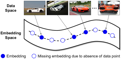
Figure 1: Illustration of the “missing embedding” issue. The data points of similar semantics are mapped into the nearby embedding space that is often with barren area due to the absence of data points, resulting in the “missing embedding” issue 

1 Introduction

Deep Metric learning (DML) is the foundation of various applications, including face recognition, verification [10, 42], image retrieval [21], image clustering [17], image classification [12], few-shot learning [32], video representation learning [5] and sound generation [6] etc. Since it was introduced, it has sparked considerable interest in the community, where academics have offered a variety of methods [18, 36, 38, 42, 45, 53, 56] and have made substantial progress [37, 41]. The goal of DML is to learn a deep model that is capable of mapping semantically similar data points to similar embeddings in the embedding space. To accomplish this, most existing approaches [7, 18, 42, 48, 53, 56] train the deep model with loss functions that bring the embeddings from semantically similar data points close to each other and vice versa. However, some embeddings may have limited contribution or bring no improvement to train the deep model [56], or even lead to bad local minima early on in training (such as a collapsed model) [42]. Thus, sampling informative and stable embeddings is very important to facilitate the training of deep model [56]. As a result, improving the sample quality is of significance to achieve effective DML. There are two commonly used measures for this goal: designing more effective sampling methods or providing more embeddings.

Pioneering efforts have made substantial progress toward the design of effective sampling methods upon embedding pairs [41, 42, 56] or a full batch of embeddings [36, 38]. These methods typically perform sampling on a batch of embeddings, which often leads to inaccurate sampling results due to the following reasons. First, the batch size is typically constrained by the memory of a single GPU as the sampling process typically cannot cross different GPU devices [41]. Second, even with GPU that has sufficient memory to support a larger batch size, the embedding space that contains the embeddings embedded by deep models may still with barren area due to the absence of data points, resulting in a “missing embedding” issue (as shown in Fig. 1). Thus, the limited amount of embeddings may impair the sample quality and the performance of DML. Based on the above analyses, we ask: “Can we overcome the inaccurate sampling issue brought by the absence of data points?”

Very recently, a few attempts [13, 16, 28, 54, 64] have been committed to answering this question by pseudo embedding generation. Hard example generation approaches [13, 64] generate hard embeddings from easy embeddings with an additional generative adversarial network or auto-encoder. Embedding expansion [28] performs interpolation between embeddings to achieve augmentation in embedding space. Cross batch memory [54] maintains embeddings from previous iterations and considers them are still informative in the current batch in terms of sampling. However, these approaches either leverage additional sub-network [13, 64], which introduce extra training cost, or need further modification to the sampling and loss computation process [28, 54] in standard DML [18, 20, 42, 45, 53], which may limit their applicability to other tasks.

In this paper, we seek to densely produce embeddings without data points to alleviate the “missing embedding” issue. In this way, with the combination of embeddings with and without data points, we are able to provide more embeddings for sampling to improve the sample quality and achieve effective DML. Our motivation stems from a fundamental hypothesis of metric learning: the embeddings that are close to each other in the embedding space have similar semantics. Unfortunately, how to exploit the embedding space to produce effective embeddings without data points remains an unsolved problem. To this end, we propose a Densely-Anchored Sampling (DAS) scheme to consider the embedding with data point as “anchor” and densely exploit the anchor’s nearby embedding space to produce embeddings that have no corresponding data points. The proposed DAS is consist of two modules, namely, Discriminative Feature Scaling (DFS) and Memorized Transformation Shifting (MTS), which exploit the embedding space around single and multiple embeddings respectively to produce effective embeddings with no corresponding data points. To be specific, based on observations that effective semantics for one embedding are highly activated features [2, 3, 14], DFS identifies these features and applies random scaling on them. In this sense, we are able to exploit the embedding space around a single embedding by enhancing or weakening its effective semantics to produce embeddings. Based on the fact that semantic differences (i.e., transformations) of intra-class embeddings can be added to other embeddings to generate effective embeddings [31], we assume that they can be added in a way like word embeddings [34]: $\text{Queen}=\text{Woman}+(\text{King}-\text{Man})$. Thus, our Memorized Transformation Shifting module exploits the embedding space among multiple embeddings by adding (i.e., shift) intra-class embeddings’ semantic differences to other embeddings of the same class to produce effective embeddings.

Our main contributions are summarized as follows. First, we propose a novel and plug-and-play Densely-Anchored Sampling (DAS) scheme that exploits embeddings’ nearby embedding space and densely produces embeddings without data points to improve the sampling quality and performance of DML. Second, we propose two modules, namely Discriminative Feature Scaling (DFS) and Memorized Transformation Shifting (MTS) to exploit embedding space around a single and multiple embeddings to produce embeddings. Last, extensive experiments demonstrate the effectiveness of the proposed method.

2 Related Work

Sampling Methods in DML. Sampling informative and stable embeddings is vital to train the deep model in DML [41, 42, 56]. Thus, various sampling approaches [15, 41, 42, 53, 56] have been tailored to effectively sample the embeddings to train the deep model. To further improve sampling efficiency, some researchers propose to leverage a whole batch of embeddings [20, 25, 36, 53, 67]. Even though sophisticated sampling methods improve DML, due to the absence of data points, sampling embeddings that are often with “missing embedding” leads to inaccurate sampling, thereby degenerating the final performance. In this paper, we propose a DAS scheme to produce embeddings with no data points by exploiting embeddings’ nearby embedding space to achieve effective DML.

Loss Functions for DML. Studies on DML losses can be grouped into two categories: pair-based and proxy-based. The pair-based losses [18, 22, 26, 42, 45, 51, 52, 53, 56, 58] are constructed upon the pairwise distance between embeddings. Although pair-based approaches mine the rich information among vast embedding pairs, they typically encounter the sampling effective embedding pairs issues. Instead, proxy-based [1, 10, 25, 33, 36, 40, 60] losses introduce the concept of “proxy” as a class representation and avoid the sampling issue by optimizing the embedding close to its proxy. However, proxy-based methods are very difficult to train when the number of classes is extremely large [38], limiting their applicability to real-life scenarios. Thus, in this paper, we focus on developing an effective technique to alleviates the general data sampling issue for pair-based methods that have wider applicability and delivers boosted performance for them.

Pseudo Embedding Generation. Methods on synthesizing pseudo embedding have been recently shown as an important technique to improve DML [13, 28, 31, 54, 62, 64]. DAML [13] uses an additional generative adversarial network to generates only hard negatives to improve the model training. HDML [62] leverages the inter-class information for embedding generation on the sampled embeddings. DVML [31] apply extra generator and decoder to model the class centers that may have inaccurate distance estimation to the real embeddings and employs them to generate embeddings. Embedding expansion [28] linearly interpolates the embeddings to obtain more embeddings. Cross batch memory [54] stores embeddings from previous batches and considers them beneficial for the upcoming sampling process. However these approaches [28, 54] suffer from the following limitations: First, the generated embeddings can only be considered as negative during sampling, which may limit the power of them. Second, the sampling or loss computation process need to be modified to dock with them, limiting their applicability. Third, an additional sub-network is introduced in order to generate embeddings, which brings heavy computation cost. Last, information source that may have inaccurate distance measurement to real embeddings such as class centers and inter-class differences are considered to produce embeddings. Different from them, DAS is a light-weight module, which produces embeddings by densely sampling around the “anchor” and serves as a plug-and-play component to facilitate the sampling process in standard DML.

Data Augmentation. Augmentation in data space such as image [44] has been widely studied and is considered an important technique to avoid overfitting. Recently, many efforts have been made to design effective augmentation methods [11, 8, 49, 55, 57] in feature space, aiming to provide more features for training when the source data (e.g., images) is scarce. These methods often introduce complicated training processes [8, 49]. Wang et al.  [55] propose ISDA that estimates semantic differences with covariance matrices and develops an improved version of cross-entropy loss. The computation and memory consumption of covariance matrices are much heavier than DAS. Moreover, ISDA can not be trivially extended to pair-based DML loss. Yin et al.  [57] introduce FTL that requires extra networks (e.g., decoder and feature transfer module) and a carefully designed bi-stage training strategy to achieve feature translation, which is less efficient and general than DAS. Unlike these methods, we view the feature space augmentation as an approach to fill the “missing embedding” in the embedding space and propose a simpler solution under the context of DML.

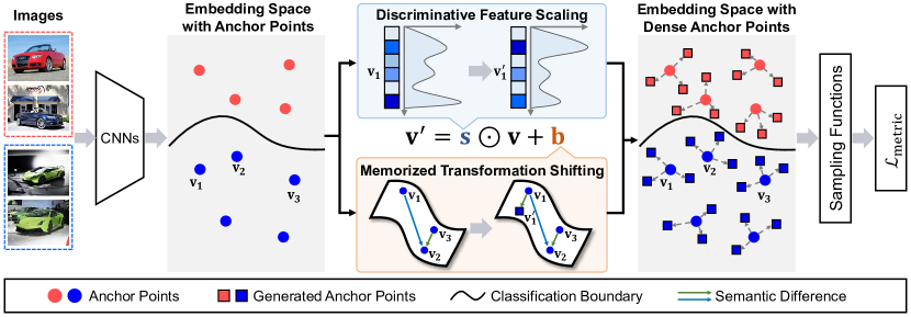
Figure 2: Illustration of our Densely-Anchored Sampling (DAS) scheme, which leverages two modules to exploit anchors’ (i.e., embeddings with data points) nearby embedding space to densely produce embeddings without data points: DFS performs random scaling on the discriminative features to produce embeddings around a single embedding; MTS exploits the embedding space among multiple embeddings by adding the intra-class semantic differences to embeddings of the same class to produce embeddings. With DAS, we alleviate the “missing embedding” issue by providing more embeddings for sampling, thereby, achieving effective DML 

3 Densely-Anchored Sampling

In this paper, we seek to improve DML by alleviating the “missing embedding” issue incurred in sampling. The overall process of DAS scheme is shown in Fig. 2.

Notation. Let ${\bf v}=f_{\theta}({\bf I})\in{\mathbb{R}}^{d}$ be an embedding with data point ${\bf I}$, where $f_{\theta}(\cdot)$ is a deep model (e.g., CNNs) with learnable parameters $\theta$. Let $y_{{\bf v}}$ be the label of the embedding ${\bf v}$. Let ${\bf v}^{\prime}$ denote embedding without data point. Following previous methods [42], we normalize both ${\bf v}$ and ${\bf v}^{\prime}$ to the $d$-dimensional hyper-sphere (i.e., $\|{\bf v}\|_{2},\|{\bf v}^{\prime}\|_{2}=1$). We omit the normalization process for brevity. Let $C$ denote the number of training classes.

3.1 Problem Definition and Motivation

DML seeks to learn a deep model that keeps similar data points close, and vice versa. Formally, we define the distance between two embeddings as follows [56]:

$${\bf D}_{ij}=\|f_{\theta}({\bf I}_{i})-f_{\theta}({\bf I}_{j})\|,$$ (1)

where $\|\cdot\|$ denotes the $\ell_{2}$ norm. For any positive pair of embeddings ($y_{i}=y_{j}$), the distance should be small; Whilst for negative pair ($y_{i}\neq y_{j}$), it should be large. In practice, limited by computing resources, it is infeasible to optimize every element in ${\bf D}_{ij}$. Therefore, it is necessary to sample effective embedding pair for the objective construction (take the contrastive loss as an example):

$${\mathcal{L}}=\sum_{(i,j)\in{\mathcal{Q}}}{\mathbb{I}}\{y_{i}=y_{j}\}~{}{\bf D}_{ij}+{\mathbb{I}}\{y_{i}\neq y_{j}\}~{}[\alpha-{\bf D}_{ij}]_{+},$$ (2)

where ${\mathbb{I}}\{\cdot\}$ is the indication function, $\alpha$ is a margin, ${\mathcal{Q}}=\operatorname{S}(D)$ indicates indexes of the sampled embedding pairs and $\operatorname{S}$ denotes some sampling function.

Without causing ambiguity, we denote the points on the embedding space as “anchor points”, based on which we will conduct sampling to train the deep model. Note that each data point shall have an anchor point on the embedding space. However, due to the absence of training data, the embedding space may have a lot of “barren area”. Thus, it is very difficult to provide sufficient anchor points for sampling and learn a deep model with good performance. To this end, we propose to densely produce anchor points with no data points to facilitate the sampling, thereby improving the training in DML.

Specifically, we first propose to exploit the embedding space around a single embedding by enhancing or weakening its semantics. We term this process as semantic scaling. Second, we propose to add (i.e., shift) intra-class differences (i.e., transformations) to embeddings to exploit the embedding space among multiple embeddings. We term this process as semantic shifting. Based on the above analyses, the formulation of DAS scheme is formulated as

$${\bf v}^{\prime}=\operatorname{DAS}({\bf v};~{}{\bf s},{\bf b})=\underbrace{{\bf s}~{}\odot~{}{\bf v}}_{\emph{scaling}}\underbrace{+~{}~{}{\bf b}}_{\emph{shifting}},$$ (3)

where ${\bf v}$ and ${\bf v}^{\prime}$ are embeddings with and without data points, respectively. $\odot$ denotes the Hadamard product. ${\bf s},{\bf b}\in{\mathbb{R}}^{d}$ are semantic scaling and semantic shifting factors, respectively. Moreover, given a set of semantic scaling and shifting factor pairs $\{({\bf s}_{t},{\bf b}_{t})\}$, we are able to produce a set of embeddings by

$${\bf v}^{\prime}_{t}=\operatorname{DAS}({\bf v};~{}{\bf s}_{t},{\bf b}_{t}).$$ (4)

Therefore, the semantic scaling and shifting factors is essential to the quality of the produced embeddings and we propose DFS and MTS to acquire them:

$${\bf s} =\operatorname{DFS}(\{{\bf v}\mid y_{{\bf v}}=c\}),$$ (5)

$${\bf b} =\operatorname{MTS}(\{{\bf v}\mid y_{{\bf v}}=c\}),$$ (6)

where DFS and MTS take embeddings from the same class as input and produce the semantic scaling and shifting factors, respectively.

3.2 Discriminative Feature Scaling

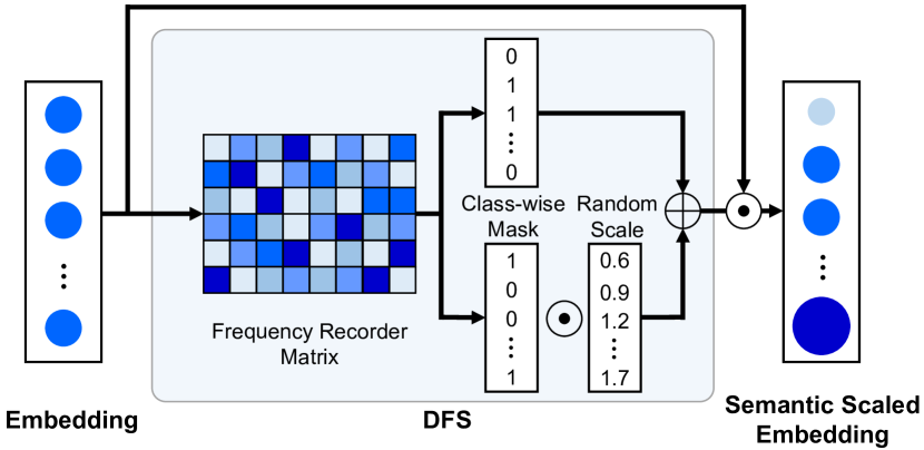
Figure 3: Illustration of the proposed Discriminative Feature Scaling (DFS) module, which identifies the discriminative features (e.g., channels) and applies different random scaling to them to produce embeddings around a single embedding 

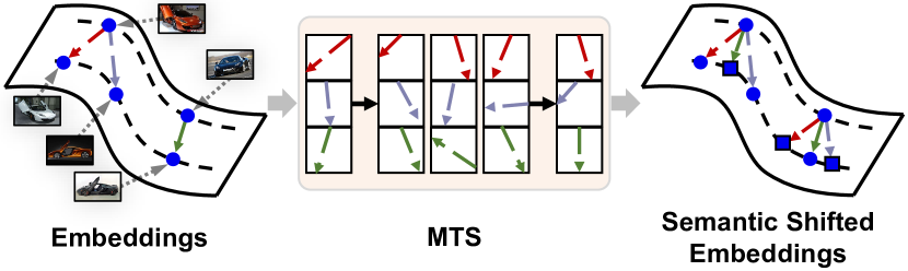
Figure 4: Illustration of the proposed Memorized Transformation Shifting (MTS) module. MTS adds the intra-class transformations to embeddings of the same class to produce embeddings among multiple embeddings 

We seek to obtain effective semantic scaling factors to produce anchor points around a single anchor. Thus, as shown in Fig. 4, our Discriminative Feature Scaling (DFS) module carries out the semantic scaling mechanism by finding the discriminative features in an embedding and applying random scaling on them. The feasibility of DFS comes from two aspects. First, visual attributes can be predicted reliably using a sparse number of neurons from CNNs [14]. Second, in CNNs, neurons that match a diverse set of object concepts are highly activated [2, 3]. In practice, the embedding typically occupies a high dimensional embedding space, which contains semantics for all training classes and semantics for each class are diverse. Thus, the semantics for one class are more likely to be noise for another. In this sense, it is very important to find out the effective e.g., discriminative features for each class in order to perform semantic scaling. To this end, we propose to identify the effective semantics by counting the number of occurrences of the highly-activated neurons for each class.

To be specific, we first initialize a Frequency Recorder Matrix (FRM) ${\bf P}\in{\mathbb{R}}^{C\times d}$ as a zero matrix. Then, given a set of embeddings $\{{\bf v}\mid y_{{\bf v}}=c\}$ from class $c$, we update ${\bf P}$ as follows:

$${\bf P}[c,k]=\left\{\begin{aligned} &{\bf P}[c,k]+1,&\text{ if }{\bf v}[k]\in\operatorname{Top}({\bf v},K),\\ &{\bf P}[c,k],&\text{ otherwise, }\end{aligned}\right.$$ (7)

where $\operatorname{Top}({\bf v},K)$ is an operator to select the top-$K$ elements from the vector ${\bf v}$. During training, we constantly update the FRM by recording the position of highly-activated neurons from the embeddings of the same class. In this way, FRM serves as a stable, accurate and effective semantics identifier for training classes. Given the FRM, we compute the class-wise binary channel mask ${\bf M}\in{\mathbb{R}}^{C\times d}$ by

$${\bf M}[c,k]=\left\{\begin{aligned} &1,&\text{ if }{\bf P}[c,k]\in\operatorname{Top}({\bf P}[c],K),\\ &0,&\text{ otherwise. }\end{aligned}\right.$$ (8)

Given an embedding ${\bf v}$, we attain the semantic scaling factor by

$${\bf s}={\bm{\gamma}}\odot{\bf M}[y_{{\bf v}}]{\color[rgb]{0,0,0}~{}+~{}\mathbf{1}^{d}\odot(1-{\bf M}[y_{{\bf v}}])},$$ (9)

where ${\bm{\gamma}}\in{\mathbb{R}}^{d}$ and ${\bm{\gamma}}\sim\operatorname{Uniform}[1-r_{s},1+r_{s}]^{d}$ and $r_{s}\in(0,1)$ is a hyper-parameter to be set. Note that we only randomly scale the discriminative features while leaving the indiscriminative ones intact. To produce more than one scaling factor, we repeatedly sample ${\bm{\gamma}}$ from the uniform distribution.

3.3 Memorized Transformation Shifting

To produce anchors without data points among multiple anchors, we propose a module to provide effective semantic shifting factors. As shown in Fig. 4, our Memorized Transformation Shifting (MTS) module exploit intra-class embeddings’ nearby embedding space by leveraging the differences between embeddings and adding them to other embeddings of the same class. On the basis of that semantic differences of embeddings can be added to other embedding to generate effective embeddings [31], the motivation of our MTS comes from the semantic relations of word embedding [34]: $\text{Woman}+(\text{King}-\text{Man})=\text{Queen}$, where a “woman” pluses “royal” semantics (e.g., transformation) becomes a “Queen”.

The transformations from both inter-class and intra-class embeddings are candidates for our design choices. However, the majority of the inter-class transformations typically are not transferable due to large inter-class differences. Thus, we only consider intra-class embeddings to attain the transformations. As suggested by the latest research [41], sampling only two images for each class in a batch consistently achieves good performance, which leads to very limited transformations we can obtain in one batch i.e., two transformations. To address this issue, we construct a bank to memorize the transformations from previous iterations to ensure the diversity of the transformations. Specifically, we construct a transformation bank ${\bf B}\in{\mathbb{R}}^{C\times Z\times d}$, where $Z$ is the bank capacity for each class. Then, during training, once we obtain a set of embeddings ${\mathcal{V}}_{c}=\{{\bf v}\mid y_{{\bf v}}=c\}$ from the class $c$, we calculate the transformations between them by

$${\bf t}_{z}={\bf v}_{i}-{\bf v}_{j},~{}~{}{\bf v}_{i},{\bf v}_{j}\in{\mathcal{V}}_{c},i\neq j.$$ (10)

Then, the transformations are en-queued into ${\bf B}$ according to the FIFO principle to ensure that the transformations in the bank are in a relatively fresh state:

$${\bf B}[y_{{\bf v}},z]={\bf t}_{z},~{}z\in\{1,2,\dots,Z\}.$$ (11)

Note that $z$ is reset to 1 when it reaches $Z$. Finally, with the assistance of the bank ${\bf B}$, given an embedding v, we retrieve the semantic shifting factor as follow

$${\bf b}=r_{b}{\bf t},~{}~{}{\bf t}\sim\{{\bf B}[y_{{\bf v}},z]~{}\mid~{}z\small{=}{1,2,\dots,Z}\}.$$ (12)

$r_{b}$ is a hyper-parameter. Multiple shifting factors are formed by repeat sampling.

Algorithm 1 Training method of DAS-based DML

0:  Training image-label pairs ${\mathcal{S}}=\{({\bf I}_{i},y_{i})\}_{i=1}^{N}$; the embedding function $f_{\theta}$; number of embeddings to produce $T$; number of training classes $C$; transformation bank capacity $Z$; learning rate $\alpha$.

0:  Optimized embedding function $f_{\theta}^{*}$.

1:  Initialize $\theta$ from ImageNet pretrained model.

2:  Initialize the frequency recorder matrix ${\bf P}\in{\mathbb{R}}^{C\times d}=\textbf{0}$.

3:  Initialize the transformation bank ${\bf B}\in{\mathbb{R}}^{C\times Z\times d}=\textbf{0}$.

4:  while not converge do

5:     Obtain a batch image-label pairs $\{({\bf I}_{i},y_{i})\}_{i=1}^{B}$ from ${\mathcal{S}}$.

6:     Compute embeddings ${\bf v}_{i}\leftarrow f_{\theta}({\bf I}_{i}),i=1,2,\cdots,B$.

7:     // perform semantic scaling by Discriminative Feature Scaling

8:     Update the frequency recorder matrix ${\bf P}$ by Eqn. (7).

9:     Acquire semantic scaling factors $\{{\bf s}_{j}\}_{j=1}^{B\times T}$ by Eqn. (9).

10:     // perform semantic shifting by Memorized Transformation Shifting

11:     Obtain intra-class transformations $\{{\bf t}\}$ by Eqn. (10).

12:     Update the transformation bank ${\bf B}$ by Eqn. (11).

13:     Attain semantic shifting factors $\{{\bf b}_{j}\}_{j=1}^{B\times T}$ by Eqn. (12).

14:     // perform densely-anchored sampling

15:     Produce embeddings $\{{\bf v}_{j}^{\prime}\}_{j=1}^{B\times T}$ by Eqn. (4).

16:     Sample positive and negative embedding sets.

17:     Compute the training loss ${\mathcal{L}}_{\text{{\color[rgb]{0,0,0}DAS-DML}}}$ by Eqn. (13).

18:     Update the parameters $\theta$ by $\theta\leftarrow\theta-\alpha\nabla_{\theta}{\mathcal{L}}_{\text{{\color[rgb]{0,0,0}DAS-DML}}}$.

19:  end while

3.4 DML with Densely-Anchored Sampling

The overall algorithm of integrating DAS into DML is detailed in Algorithm 1. Given anchor-label pairs $\{({\bf v},y_{{\bf v}})\}$, we produce embedding-label pairs $\{({\bf v}^{\prime},y^{\prime}_{{\bf v}})\}$ with no data points by DAS scheme, where $y^{\prime}_{{\bf v}}=y_{{\bf v}}$ since the class semantic is preserved. Then, embedding-label pairs with or without data points are fed into the sampling module to obtain the positive and negative embedding sets (e.g., pairs, triplets, etc. specified by the sampling and loss functions): $\{({\mathcal{P}},{\mathcal{N}})\}=\operatorname{Sample}(\{({\bf v},y_{{\bf v}})\}\cup\{({\bf v}^{\prime},y^{\prime}_{{\bf v}})\})$. Last, given a DML loss function ${\mathcal{L}}_{\text{DML}}$, DAS-based DML objective function is formulated as:

$${\mathcal{L}}_{\text{{\color[rgb]{0,0,0}DAS-DML}}}={\mathcal{L}}_{\text{DML}}(\{({\mathcal{P}},{\mathcal{N}})\}).$$ (13)

Table 1: Comparisons with SoTA methods on CUB, CARS and SOP. The best results are in bold. $*$ indicates the reimplementation by [4]. † denotes our reimplementation 

Method	Backbone	CUB				CARS				SOP
		R@1	R@2	R@4	R@8	R@1	R@2	R@4	R@8	R@1	R@10	R@100	R@1000
Margin [56]	$\operatorname{R}^{128}$	63.60	74.40	83.10	90.00	79.60	86.50	91.90	95.10	72.70	86.20	93.80	98.00
HDC [59]	$\operatorname{G}^{384}$	53.60	65.70	77.00	85.60	73.70	83.20	89.50	93.80	69.50	84.40	92.80	97.70
A-BIER [39]	$\operatorname{G}^{384}$	57.50	68.70	78.30	86.20	82.00	89.00	93.20	96.10	74.20	86.90	94.00	97.80
ABE [27]	$\operatorname{G}^{512}$	60.60	71.50	79.80	87.40	85.20	90.50	94.00	96.10	76.30	88.40	94.80	98.20
HTL [15]	$\operatorname{IBN}^{512}$	57.10	68.80	78.70	86.50	81.40	88.00	92.70	95.70	74.80	88.30	94.80	98.40
RLL-H [52]	$\operatorname{IBN}^{512}$	57.40	69.70	79.20	86.90	74.00	83.60	90.10	94.10	76.10	89.10	95.40	N/A
SoftTriple [40]	$\operatorname{IBN}^{512}$	65.40	76.40	84.50	90.40	84.50	90.70	94.50	96.90	78.30	90.30	95.90	N/A
MS [53]	$\operatorname{IBN}^{512}$	65.70	77.00	86.30	91.20	84.10	90.40	94.00	96.50	78.20	90.50	96.00	98.70
ProxyGML [67]	$\operatorname{IBN}^{512}$	66.60	77.60	86.40	N/A	85.50	91.80	95.30	N/A	78.00	90.60	96.20	N/A
ProxyAnchor [25]	$\operatorname{IBN}^{512}$	68.40	79.20	86.80	91.60	86.10	91.70	95.00	97.30	79.10	90.80	96.20	98.70
Contrastive + XBM [54]	$\operatorname{IBN}^{512}$	65.80	75.90	84.00	89.90	82.00	88.70	93.10	96.10	79.50	90.80	96.10	98.70
MS∗ [53]	$\operatorname{IBN}^{512}$	64.50	76.20	84.60	90.50	82.10	88.80	93.20	96.10	76.30	89.70	96.00	98.80
MS + EE∗ [28]	$\operatorname{IBN}^{512}$	65.10	76.80	86.10	91.00	82.70	89.20	93.80	96.40	77.00	89.50	96.00	98.80
ProxyAnchor + MemVir [4]	$\operatorname{IBN}^{512}$	69.00	79.20	86.80	91.60	86.70	92.00	95.20	97.40	79.70	91.00	96.30	98.60
MS† [53]	$\operatorname{IBN}^{512}$	65.72	77.19	85.74	91.56	83.86	90.41	94.64	96.99	76.89	89.58	95.59	98.60
MS + DAS ($K=8$) (Ours)	$\operatorname{IBN}^{512}$	67.07	78.11	86.43	91.88	85.66	91.60	95.27	97.37	78.16	90.26	95.99	98.76
MS† [53]	$\operatorname{R}^{512}$	66.46	77.28	85.85	91.69	83.99	90.39	94.51	96.80	79.53	91.06	96.30	98.83
MS + DAS ($K=8$) (Ours)	$\operatorname{R}^{512}$	69.19	79.25	87.09	92.62	87.84	93.15	95.99	97.85	80.59	91.80	96.68	98.95

4 Experiments

Datasets. We use three popular benchmarks: 1) CUB2011-200 (CUB) [50], a fine-grained bird dataset with the first 100 categories for training and another 100 categories for testing. 2) CARS196 (CARS) [29], a fine-grained vehicle dataset with the first 98 classes for training and another 98 classes for testing. 3) Stanford Online Products (SOP) [38], a large-scale online products dataset with the train and test partitions as 11,318 classes and another 11,316 classes, respectively.

Implementation details We leverage two popular backbones: ResNet50 [19] ($\operatorname{R}^{d}$) and Inception BN [23] ($\operatorname{IBN}^{d}$), where their parameters are initialized from ImageNet [9] pre-trained models and $d$ denotes the embedding dimension. Note that some approaches also consider GoogleNet [46] ($\operatorname{G}^{d}$) as the backbone. Here, we mainly consider the settings of $d=128,512$. $\operatorname{R}^{128}$ is used as the default backbone. The embedding layer is randomly initialized. Regarding evaluation metrics, Recall at k (R@k) [24], Normalized Mutual Information (NMI) [43] and F1 score (F1) [45] are used, where R@k measures the image retrieval performance while F1 and NMI measure the image clustering performance. For hyper-parameters in DAS, we set $(T,K,Z,r_{s},r_{b})=(3,4,10,1\text{e}^{-2},1\text{e}^{-2})$ by default. Our source code is publicly available at https://github.com/lizhaoliu-Lec/DAS.

Table 2: Comparisons with pair-based methods on CUB, CARS and SOP. [S] and [D] denote semi-hard and distance weighted sampling, respectively 

Method	CUB			CARS			SOP
	R@1	F1	NMI	R@1	F1	NMI	R@1	F1	NMI
Triplet [S] [42]	60.25	32.82	64.64	74.64	31.98	63.22	73.51	33.47	89.33
Triplet [S] + DAS	60.82	33.86	65.67	77.21	33.88	64.84	73.99	33.91	89.42
Triplet [D] [56]	62.68	36.39	67.03	78.86	35.80	65.85	77.54	37.10	90.05
Triplet [D] + DAS	64.28	38.16	68.06	82.63	39.14	68.12	77.95	37.64	90.18
Contrastive [D] [56]	61.65	35.23	66.58	76.03	32.77	64.09	73.13	35.60	89.78
Contrastive [D] + DAS	63.67	36.25	67.15	80.74	36.07	65.93	74.80	36.21	89.89
Margin [56]	62.61	37.33	67.58	80.10	37.85	67.15	78.69	39.20	90.50
Margin + DAS	64.50	37.86	68.04	82.29	38.22	67.94	79.14	39.52	90.56
GenLifted [20]	58.81	34.64	65.50	72.45	32.43	64.00	76.18	37.26	90.13
GenLifted + DAS	59.94	35.09	66.07	73.55	32.85	64.11	76.92	37.64	90.21
N-Pair [45]	60.55	36.94	67.19	77.35	36.26	66.74	77.71	37.13	90.15
N-Pair + DAS	62.81	38.37	68.43	79.93	38.06	68.20	77.98	37.82	90.28
MS [53]	62.63	38.88	68.19	82.04	40.85	69.45	78.89	37.53	90.12
MS + DAS	64.13	39.18	69.08	83.31	42.78	70.77	79.44	38.77	90.40

4.1 Comparison with State-of-the-arts

In this section, we compare our method with state-of-the-art competitors to investigate the effectiveness of DAS. The results are shown in Table 4. For fair comparisons, the results of the closely related baseline EE are from the reimplementation by [4] using the stronger $\operatorname{IBN}^{512}$ backbone ($\operatorname{G}^{512}$ in the original paper). Our approach is based on MS loss and achieves superior performance on all datasets and evaluation metrics. First, when combining the $\operatorname{R}^{512}$ backbone and DAS, we are able to boost the R@1 metrics by $3.49\%$ on CUB and $1.74\%$ on CARS, which shows that DAS is able to deliver more accurate image retrieval results even with higher embedding dimension (i.e., 512). Second, for our closely relative opponent, EE, its improvements on MS are marginal, showing that simply performing interpolation to generate embeddings is inferior to DAS. Last, even for a strong baseline, ProxyAnchor that leverages the advanced training techniques, and sophisticated loss, we still outperform it considerably.

4.2 Effectiveness of DAS on Pair-based Loss

Quantitative results. To investigate the efficacy of DAS, we conduct experiments with $\operatorname{R}^{128}$ backbone on the widely used pair-based losses. We reimplement all baselines under the same settings for a fair comparison. The results are presented in Table 2. For considered pair-based losses, DAS is able to improve their performance on both image retrieval and clustering metrics. Notably, for approaches such as GenLifted and N-Pair that leverage the whole batch of embeddings for loss computation, DAS still improves their performance, showing its effectiveness. Last, even for a very strong baseline, MS, that considers different kinds of relationships among embedding pairs and designs sophisticated weighting mechanism, DAS is able to greatly improve it without bells and whistles.

Convergence analyses. We provide the results of training loss and test set R@1 in Fig. 5 to analyze the training behaviors of DAS. The loss curve with DAS decreases smoother than that without DAS, showing that DAS provides more embeddings to facilitate sampling, thereby, stabilizing the training. Moreover, with DAS, the training loss is higher than the baseline, one possible reason is that DAS is able to act as a regularizer to avoid overfitting, which is consistent with the result that DAS achieves a higher test set R@1. Similar phenomenon is also observed in other embeddings generation methods [28].

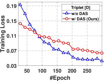
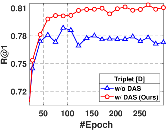
Figure 5: The training loss and test set R@1 on CARS. The sampling method and loss function are triplet loss and distance weighted sampling, respectively 

Table 3: Comparisons with various sampling methods on CARS 

Method	Sampling	DAS	R@1	F1	NMI
Triplet	Random		74.21	33.41	64.28
		✓	76.79	35.21	65.49
	Semi-hard [42]		74.64	31.98	63.22
		✓	77.10	33.82	65.03
	Soft-hard [41]		79.20	35.55	66.08
		✓	80.54	37.52	66.77
	Distance [56]		78.86	35.80	65.85
		✓	81.34	37.27	67.21
Contrastive	Random		42.44	15.83	48.87
		✓	50.79	19.40	52.71
	Distance [56]		76.03	32.77	64.09
		✓	80.70	35.47	66.01

Table 4: Comparisons with more related works on CARS 

Method	Backbone	R@1	R@2	R@4	R@8
N-Pair + HDML [63]	$\operatorname{G}^{512}$	68.90	78.90	85.80	90.90
N-Pair + HDML-A [63]	$\operatorname{G}^{512}$	81.10	88.80	93.70	96.70
N-Pair + DAS (Ours)	$\operatorname{G}^{512}$	83.70	90.33	94.47	96.77
MS + SEC [61]	$\operatorname{IBN}^{512}$	85.73	91.96	95.51	97.54
MS + DAS (Ours)	$\operatorname{IBN}^{512}$	85.66	91.60	95.27	97.37
MS + SEC + DAS (Ours)	$\operatorname{IBN}^{512}$	87.80	93.16	96.18	98.01
Margin + DiVA [35]	$\operatorname{IBN}^{512}$	83.10	90.00	N/A	N/A
Margin + DAS (Ours)	$\operatorname{IBN}^{512}$	84.85	90.32	93.99	96.40
ProxyNCA++ [47]	$\operatorname{R}^{512}$	86.50	92.50	95.70	97.70
Margin + DiVA	$\operatorname{R}^{512}$	82.20	89.00	N/A	N/A
Margin + DRML [66]	$\operatorname{R}^{512}$	73.30	83.00	89.80	94.40
Margin + DCML [65]	$\operatorname{R}^{512}$	85.20	91.80	96.00	98.00
Margin + DAS (Ours)	$\operatorname{R}^{512}$	88.34	93.21	95.92	97.59

4.3 Effectiveness of DAS on Sampling Method

In this section, we investigate the effectiveness of DAS by evaluating it with different sampling approaches. We choose two popular loss functions: triplet and contrastive losses that are sensitive to the sampling methods. Therefore, various sampling approaches are tailored for them. The experiment results are presented in Table 4. For two loss functions, despite the choice of sampling approaches, DAS is able to improve them considerably on both image retrieval and clustering metrics. Notably, when applying DAS, triplet loss with random sampling outperform the one with the semi-hard sampling. This indicates that producing more embeddings for sampling is as important as the sampling approach.

4.4 Qualitative Results

To better understand our method, we compare contrastive loss (with distance weighted sampling) w/ or w/o DAS and visualize image retrieval results on both CARS (Fig. 6) and SOP (Fig. 6) datasets. On CARS, the model performs better with DAS despite the background noises or the interference from the car’s color, demonstrating that DAS enforces the model to focus on real semantics. On SOP, the model with DAS is insensitive to drastic viewpoint changes. These results verify the generalization ability and robustness of DAS under various scenes.

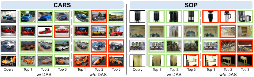
Figure 6: Top 3 retrieved results from the $\operatorname{R}^{128}$ trained w/ or w/o DAS. green and red rectangles indicate desired and undesired results, respectively 

4.5 Ablation Studies

Effect of DFS and MTS. In this section, we perform ablation studies to evaluate the performance gain by each module in DAS. The loss function and sampling method are triplet loss and distance weighted sampling, respectively. The results are in Table 5. First, DFS, alone, boosts R@1 by +2.42%, verifying that producing embeddings around a single embedding is able to force the model to focus on real semantics and achieve better image retrieval results. Second, with MTS only, the clustering metrics are greatly improved, indicating that producing embeddings among multiple embeddings are beneficial to the image clustering task. Last, with DFS and DAS, all metrics are further improved, suggesting that DFS and MTS reinforce and complement each other.

Table 5: Ablation studies on CARS 

DFS	MTS	R@1	F1	NMI
		78.86	35.80	65.85
✓		81.28 (+2.42)	36.22 (+0.42)	66.84 (+0.99)
	✓	81.83 (+2.97)	38.26 (+2.46)	67.81 (+1.96)
✓	✓	82.63 (+3.77)	39.14 (+3.34)	68.12 (+2.27)

Effect of $K$ in DFS. Multi-dimensional embeddings have a diverse set of semantic features [2, 3]. The top-K mask is effective to discover the discriminative features. We perform experiments on SOP, a large-scale and diverse dataset with margin loss to support our claim. With $K=1,2,4,8,16,32$, we obtain results $\text{R@1}=78.76,78.86,\textbf{79.14},78.09,77.94,77.96$, where substantial improvements are observed when $K=\{1,2,4\}$ and larger $K~{}(\text{\emph{i.e.,}}~{}K>4)$ leads to worse results.

Effect of $Z$ in MTS. The larger bank capacity ($Z$) allows us to access intra-class transformations from current and previous iterations, which improves the diversity of the produced embeddings. We conduct experiments on CARS with margin loss by setting $Z=1,2,3,4,5$ and obtain $\text{R@1}=82.35,82.38,82.42,\textbf{82.75},82.33$, showing that history transformations ($Z>2$) bring slight improvements.

4.6 Further Discussions

More discussions on DFS. One may question whether the proposed DFS requires the linear assumption on high dimensional feature space. In fact, we do not make this assumption and our method is built on a very basic hypothesis of metric learning: the embeddings that are close to each other in the embedding space have similar semantics. More critically, DFS does not rely on the linearity assumption. Instead, DFS is based on the observations that effective semantics for one embedding are highly activated features [2, 3].

More discussions on MTS. Li et al.  [30] also apply a memory module is leveraged to store abundant features and conduct neighborhood search upon them to enhance the discriminative power of a general CNN feature on the image search and few-shot learning tasks. Unlike them, DAS constructs a memory bank with the intra-class embedding transformations, which allows us to access intra-class transformations from current and previous iterations, and thus improves the diversity of produced embeddings for DML.

Comparisons with more related works. In Table 4, we compare DAS with HDML [63], SEC [61], DiVA [35], ProxyNCA++ [47], DRML [66], DCML [65] on CARS under the same settings. We can see that DAS outperforms HDML, DiVA, DRML and DCML, and achieves comparable performance to SEC. Note that DAS can be also incorporated into SEC. As a result, using MS loss, SEC + DAS outperforms SEC by 2.07% in R@1. These results further verify the applicability of DAS on some regularization techniques in DML.

5 Conclusion

In this paper, we propose a Densely-Anchored Sampling (DAS) scheme to alleviate the “missing embedding” issue incurred during DML sampling. To this end, we propose to produce embeddings with no data points by exploiting the embeddings’ nearby embedding space. Specifically, we propose a DFS module that identifies an embedding’s discriminative features and performs random scaling on them to exploit the embedding space around it. Moreover, we propose a MTS module to exploit embedding space among multiple embedding by adding the intra-class semantic differences to embeddings of the same class. By combining the embeddings with and without data points, DAS provides more embeddings for sampling to improve the sampling quality and achieve effective DML. Extensive experiments with various loss functions and sampling methods on three public available benchmarks show that DAS is effective. In the future, we plan to apply DAS to other areas such as self-supervised learning that require sampling.

Acknowledgements. This work was partially supported by Peng Cheng Laboratory Research Project No. PCL2021A07, National Natural Science Foundation of China (NSFC) 62072190, Program for Guangdong Introducing Innovative and Enterpreneurial Teams 2017ZT07X183.

See pages 1 of 3844-supp.pdf See pages 2 of 3844-supp.pdf See pages 3 of 3844-supp.pdf See pages 4 of 3844-supp.pdf See pages 5 of 3844-supp.pdf See pages 6 of 3844-supp.pdf See pages 7 of 3844-supp.pdf See pages 8 of 3844-supp.pdf See pages 9 of 3844-supp.pdf See pages 10 of 3844-supp.pdf See pages 11 of 3844-supp.pdf See pages 12 of 3844-supp.pdf See pages 13 of 3844-supp.pdf See pages 14 of 3844-supp.pdf

References

- [1] Aziere, N., Todorovic, S.: Ensemble deep manifold similarity learning using hard proxies. In: Proceedings of the IEEE/CVF Conference on Computer Vision and Pattern Recognition. pp. 7299–7307 (2019)
- [2] Bau, D., Zhou, B., Khosla, A., Oliva, A., Torralba, A.: Network dissection: Quantifying interpretability of deep visual representations. In: Proceedings of the IEEE Conference on Computer Vision and Pattern Recognition. pp. 6541–6549 (2017)
- [3] Bau, D., Zhu, J.Y., Strobelt, H., Lapedriza, A., Zhou, B., Torralba, A.: Understanding the role of individual units in a deep neural network. Proceedings of the National Academy of Sciences 117(48), 30071–30078 (2020)
- [4] Byungsoo Ko, G.G., Kim, H.G.: Learning with memory-based virtual classes for deep metric learning. In: Proceedings of the IEEE/CVF International Conference on Computer Vision (2021)
- [5] Chen, P., Huang, D., He, D., Long, X., Zeng, R., Wen, S., Tan, M., Gan, C.: Rspnet: Relative speed perception for unsupervised video representation learning. In: AAAI Conference on Artificial Intelligence, 2021 (2020)
- [6] Chen, P., Zhang, Y., Tan, M., Xiao, H., Huang, D., Gan, C.: Generating visually aligned sound from videos. IEEE Transactions on Image Processing 29, 8292–8302 (2020)
- [7] Chen, W., Chen, X., Zhang, J., Huang, K.: Beyond triplet loss: a deep quadruplet network for person re-identification. In: Proceedings of the IEEE Conference on Computer Vision and Pattern Recognition. pp. 403–412 (2017)
- [8] Chu, P., Bian, X., Liu, S., Ling, H.: Feature space augmentation for long-tailed data. In: Proceedings of the European Conference on Computer Vision. pp. 694–710. Springer (2020)
- [9] Deng, J., Dong, W., Socher, R., Li, L.J., Li, K., Fei-Fei, L.: Imagenet: A large-scale hierarchical image database. In: Proceedings of the IEEE Conference on Computer Vision and Pattern Recognition. pp. 248–255. IEEE (2009)
- [10] Deng, J., Guo, J., Xue, N., Zafeiriou, S.: Arcface: Additive angular margin loss for deep face recognition. In: Proceedings of the IEEE/CVF Conference on Computer Vision and Pattern Recognition. pp. 4690–4699 (2019)
- [11] DeVries, T., Taylor, G.W.: Dataset augmentation in feature space. arXiv preprint arXiv:1702.05538 (2017)
- [12] Ding, Z., Fu, Y.: Robust transfer metric learning for image classification. IEEE Transactions on Image Processing 26(2), 660–670 (2016)
- [13] Duan, Y., Zheng, W., Lin, X., Lu, J., Zhou, J.: Deep adversarial metric learning. In: Proceedings of the IEEE Conference on Computer Vision and Pattern Recognition. pp. 2780–2789 (2018)
- [14] Escorcia, V., Carlos Niebles, J., Ghanem, B.: On the relationship between visual attributes and convolutional networks. In: Proceedings of the IEEE Conference on Computer Vision and Pattern Recognition. pp. 1256–1264 (2015)
- [15] Ge, W.: Deep metric learning with hierarchical triplet loss. In: Proceedings of the European Conference on Computer Vision. pp. 269–285 (2018)
- [16] Gu, G., Ko, B., Kim, H.G.: Proxy synthesis: Learning with synthetic classes for deep metric learning. In: Proceedings of the AAAI Conference on Artificial Intelligence. pp. 1460–1468 (2021)
- [17] Guo, X., Gao, L., Liu, X., Yin, J.: Improved deep embedded clustering with local structure preservation. In: International Joint Conference on Artificial Intelligence. pp. 1753–1759 (2017)
- [18] Hadsell, R., Chopra, S., LeCun, Y.: Dimensionality reduction by learning an invariant mapping. In: IEEE Computer Society Conference on Computer Vision and Pattern Recognition. vol. 2, pp. 1735–1742. IEEE (2006)
- [19] He, K., Zhang, X., Ren, S., Sun, J.: Deep residual learning for image recognition. In: Proceedings of the IEEE Conference on Computer Vision and Pattern Recognition. pp. 770–778 (2016)
- [20] Hermans, A., Beyer, L., Leibe, B.: In defense of the triplet loss for person re-identification. arXiv preprint arXiv:1703.07737 (2017)
- [21] Hoi, S.C., Liu, W., Chang, S.F.: Semi-supervised distance metric learning for collaborative image retrieval and clustering. ACM Transactions on Multimedia Computing, Communications, and Applications 6(3), 1–26 (2010)
- [22] Hu, J., Lu, J., Tan, Y.P.: Discriminative deep metric learning for face verification in the wild. In: Proceedings of the IEEE Conference on Computer Vision and Pattern Recognition. pp. 1875–1882 (2014)
- [23] Ioffe, S., Szegedy, C.: Batch normalization: Accelerating deep network training by reducing internal covariate shift. In: International Conference on Machine Learning. pp. 448–456. PMLR (2015)
- [24] Jegou, H., Douze, M., Schmid, C.: Product quantization for nearest neighbor search. IEEE Transactions on Pattern Analysis and Machine Intelligence 33(1), 117–128 (2010)
- [25] Kim, S., Kim, D., Cho, M., Kwak, S.: Proxy anchor loss for deep metric learning. In: Proceedings of the IEEE/CVF Conference on Computer Vision and Pattern Recognition. pp. 3238–3247 (2020)
- [26] Kim, S., Seo, M., Laptev, I., Cho, M., Kwak, S.: Deep metric learning beyond binary supervision. In: Proceedings of the IEEE/CVF Conference on Computer Vision and Pattern Recognition. pp. 2288–2297 (2019)
- [27] Kim, W., Goyal, B., Chawla, K., Lee, J., Kwon, K.: Attention-based ensemble for deep metric learning. In: Proceedings of the European Conference on Computer Vision. pp. 736–751 (2018)
- [28] Ko, B., Gu, G.: Embedding expansion: Augmentation in embedding space for deep metric learning. In: Proceedings of the IEEE/CVF Conference on Computer Vision and Pattern Recognition. pp. 7255–7264 (2020)
- [29] Krause, J., Stark, M., Deng, J., Fei-Fei, L.: 3d object representations for fine-grained categorization. In: Proceedings of the IEEE International Conference on Computer Vision Workshops. pp. 554–561 (2013)
- [30] Li, S., Chen, D., Liu, B., Yu, N., Zhao, R.: Memory-based neighbourhood embedding for visual recognition. In: Proceedings of the IEEE/CVF International Conference on Computer Vision. pp. 6102–6111 (2019)
- [31] Lin, X., Duan, Y., Dong, Q., Lu, J., Zhou, J.: Deep variational metric learning. In: Proceedings of the European Conference on Computer Vision. pp. 689–704 (2018)
- [32] Liu, L., Cao, J., Liu, M., Guo, Y., Chen, Q., Tan, M.: Dynamic extension nets for few-shot semantic segmentation. In: Proceedings of the 28th ACM International Conference on Multimedia. pp. 1441–1449 (2020)
- [33] Liu, W., Wen, Y., Yu, Z., Li, M., Raj, B., Song, L.: Sphereface: Deep hypersphere embedding for face recognition. In: Proceedings of the IEEE Conference on Computer Vision and Pattern Recognition. pp. 212–220 (2017)
- [34] Mikolov, T., Yih, W.t., Zweig, G.: Linguistic regularities in continuous space word representations. In: Proceedings of the 2013 Conference of the North American Chapter of the Association for Computational Linguistics: Human Language Technologies. pp. 746–751 (2013)
- [35] Milbich, T., Roth, K., Bharadhwaj, H., Sinha, S., Bengio, Y., Ommer, B., Cohen, J.P.: Diva: Diverse visual feature aggregation for deep metric learning. In: European Conference on Computer Vision. pp. 590–607. Springer (2020)
- [36] Movshovitz-Attias, Y., Toshev, A., Leung, T.K., Ioffe, S., Singh, S.: No fuss distance metric learning using proxies. In: Proceedings of the IEEE International Conference on Computer Vision. pp. 360–368 (2017)
- [37] Musgrave, K., Belongie, S., Lim, S.N.: A metric learning reality check. In: European Conference on Computer Vision. pp. 681–699. Springer (2020)
- [38] Oh Song, H., Xiang, Y., Jegelka, S., Savarese, S.: Deep metric learning via lifted structured feature embedding. In: Proceedings of the IEEE Conference on Computer Vision and Pattern Recognition. pp. 4004–4012 (2016)
- [39] Opitz, M., Waltner, G., Possegger, H., Bischof, H.: Deep metric learning with bier: Boosting independent embeddings robustly. IEEE Transactions on Pattern Analysis and Machine Intelligence 42(2), 276–290 (2018)
- [40] Qian, Q., Shang, L., Sun, B., Hu, J., Li, H., Jin, R.: Softtriple loss: Deep metric learning without triplet sampling. In: Proceedings of the IEEE/CVF International Conference on Computer Vision. pp. 6450–6458 (2019)
- [41] Roth, K., Milbich, T., Sinha, S., Gupta, P., Ommer, B., Cohen, J.P.: Revisiting training strategies and generalization performance in deep metric learning. In: International Conference on Machine Learning. pp. 8242–8252. PMLR (2020)
- [42] Schroff, F., Kalenichenko, D., Philbin, J.: Facenet: A unified embedding for face recognition and clustering. In: Proceedings of the IEEE Conference on Computer Vision and Pattern Recognition. pp. 815–823 (2015)
- [43] Schütze, H., Manning, C.D., Raghavan, P.: Introduction to Information Retrieval, vol. 39. Cambridge University Press Cambridge (2008)
- [44] Shorten, C., Khoshgoftaar, T.M.: A survey on image data augmentation for deep learning. Journal of Big Data 6(1), 1–48 (2019)
- [45] Sohn, K.: Improved deep metric learning with multi-class n-pair loss objective. In: Proceedings of the 30th International Conference on Neural Information Processing Systems. pp. 1857–1865 (2016)
- [46] Szegedy, C., Liu, W., Jia, Y., Sermanet, P., Reed, S., Anguelov, D., Erhan, D., Vanhoucke, V., Rabinovich, A.: Going deeper with convolutions. In: Proceedings of the IEEE Conference on Computer Vision and Pattern Recognition. pp. 1–9 (2015)
- [47] Teh, E.W., DeVries, T., Taylor, G.W.: Proxynca++: Revisiting and revitalizing proxy neighborhood component analysis. In: European Conference on Computer Vision. pp. 448–464. Springer (2020)
- [48] Ustinova, E., Lempitsky, V.: Learning deep embeddings with histogram loss. In: Proceedings of the International Conference on Neural Information Processing Systems. pp. 4177–4185 (2016)
- [49] Volpi, R., Morerio, P., Savarese, S., Murino, V.: Adversarial feature augmentation for unsupervised domain adaptation. In: Proceedings of the IEEE Conference on Computer Vision and Pattern Recognition. pp. 5495–5504 (2018)
- [50] Wah, C., Branson, S., Welinder, P., Perona, P., Belongie, S.: The caltech-ucsd birds-200-2011 dataset (2011)
- [51] Wang, J., Song, Y., Leung, T., Rosenberg, C., Wang, J., Philbin, J., Chen, B., Wu, Y.: Learning fine-grained image similarity with deep ranking. In: Proceedings of the IEEE Conference on Computer Vision and Pattern Recognition. pp. 1386–1393 (2014)
- [52] Wang, X., Hua, Y., Kodirov, E., Hu, G., Garnier, R., Robertson, N.M.: Ranked list loss for deep metric learning. In: Proceedings of the IEEE/CVF Conference on Computer Vision and Pattern Recognition. pp. 5207–5216 (2019)
- [53] Wang, X., Han, X., Huang, W., Dong, D., Scott, M.R.: Multi-similarity loss with general pair weighting for deep metric learning. In: Proceedings of the IEEE/CVF Conference on Computer Vision and Pattern Recognition. pp. 5022–5030 (2019)
- [54] Wang, X., Zhang, H., Huang, W., Scott, M.R.: Cross-batch memory for embedding learning. In: Proceedings of the IEEE/CVF Conference on Computer Vision and Pattern Recognition. pp. 6388–6397 (2020)
- [55] Wang, Y., Pan, X., Song, S., Zhang, H., Huang, G., Wu, C.: Implicit semantic data augmentation for deep networks. Advances in Neural Information Processing Systems 32, 12635–12644 (2019)
- [56] Wu, C.Y., Manmatha, R., Smola, A.J., Krahenbuhl, P.: Sampling matters in deep embedding learning. In: Proceedings of the IEEE International Conference on Computer Vision. pp. 2840–2848 (2017)
- [57] Yin, X., Yu, X., Sohn, K., Liu, X., Chandraker, M.: Feature transfer learning for face recognition with under-represented data. In: Proceedings of the IEEE/CVF Conference on Computer Vision and Pattern Recognition. pp. 5704–5713 (2019)
- [58] Yu, B., Tao, D.: Deep metric learning with tuplet margin loss. In: Proceedings of the IEEE/CVF International Conference on Computer Vision. pp. 6490–6499 (2019)
- [59] Yuan, Y., Yang, K., Zhang, C.: Hard-aware deeply cascaded embedding. In: Proceedings of the IEEE International Conference on Computer Vision. pp. 814–823 (2017)
- [60] Zhai, A., Wu, H.Y.: Classification is a strong baseline for deep metric learning (2019)
- [61] Zhang, D., Li, Y., Zhang, Z.: Deep metric learning with spherical embedding. Advances in Neural Information Processing Systems 33, 18772–18783 (2020)
- [62] Zhao, Y., Jin, Z., Qi, G.j., Lu, H., Hua, X.s.: An adversarial approach to hard triplet generation. In: Proceedings of the European Conference on Computer Vision. pp. 501–517 (2018)
- [63] Zheng, W., Lu, J., Zhou, J.: Hardness-aware deep metric learning. IEEE Transactions on Pattern Analysis and Machine Intelligence 43(9), 3214–3228 (2021)
- [64] Zheng, W., Chen, Z., Lu, J., Zhou, J.: Hardness-aware deep metric learning. In: Proceedings of the IEEE/CVF Conference on Computer Vision and Pattern Recognition. pp. 72–81 (2019)
- [65] Zheng, W., Wang, C., Lu, J., Zhou, J.: Deep compositional metric learning. In: Proceedings of the IEEE/CVF Conference on Computer Vision and Pattern Recognition. pp. 9320–9329 (2021)
- [66] Zheng, W., Zhang, B., Lu, J., Zhou, J.: Deep relational metric learning. In: Proceedings of the IEEE/CVF International Conference on Computer Vision. pp. 12065–12074 (2021)
- [67] Zhu, Y., Yang, M., Deng, C., Liu, W.: Fewer is more: A deep graph metric learning perspective using fewer proxies. Advances in Neural Information Processing Systems 33, 17792–17803 (2020)