Addition to the Gnevyshev-Ohl rule and prediction of solar cycle 25

Abstract

In addition to the Gnevyshev-Ohl rule (GOR), the relation of the odd cycle with the subsequent even one in the 22-year Hale solar cycle was found. It is shown that 3 years before the 11-year minimum $m$, the value of the relative sunspot number $S\!N$ in an odd cycle is closely related to the value of the maximum in the next even cycle (correlation coefficient $\rho=0.94$), and the same relation of an odd cycle with the previous even one is weaker. Like GOR, cycles are linked in pairs, but opposite to the Rule.

Based on this result, we propose to use $S\!N_{m-3}$ on the descending phase of the previous odd cycle as a precursor of the subsequent EVEN cycle (Figure 3a) — a precursor called MI3E. For the prediction of an odd cycle or a prediction without consideration of parity (as in the article by brajsa22), this method gives less reliable results.

To predict the amplitude of an ODD cycle, we propose to use the precursor of the seventh year to its maximum $M$ MA7O — $S\!N_{M-7}$ on the descending phase of the previous even cycle (Figure 3b). It turned out that in this case, we can also predict the years near the maximum with a high correlation coefficient ($\rho=0.90{-}0.94$).

Thus, the proposed approaches allow us to predict cycles of different parity. According to our prediction, the current solar Cycle 25 in 2023 will reach a maximum of 154 units with a prediction error of $\pm 25$ (68% confidence) and $\pm 53$ (95% confidence). In 2024, $S\!N$ will be almost as high as in 2023 — 147 units, so with smaller time averaging scales, the maximum will fall at the end of 2023.

1 Introduction

As noted in (nag09), “The empirical Gnevyshev-Ohl rule (1948), below referred to as GOR or the Rule, is one of the most puzzling properties of the solar cyclicity.” gnevohl48, based on the consideration of a relative sunspot numbers $S\!N$ from 1700 to 1944, found that the area under the curve (total power) of the 11-year cycle $\sum S\!N$ has a high correlation for the pair of even – subsequent odd cycles and weakly correlates for the pair of odd – subsequent even cycles. Thus, they concluded that the 22-year Hale cycle begins with an even cycle. This is a strange circumstance since the resulting rule divides cycles into pairs, and neighboring pairs are weakly related. One of the questions we raise in this article is: in addition to the parameter $\sum S\!N$, are there cycle parameters that connect consecutive cycles in different ways, including in the odd – subsequent even cycle pair?

In addition, we touch on a purely practical question of solar cycle prediction: how will look the recently started Cycle 25, and what will be its amplitude when the moment of maximum comes. As it turned out, in the context under consideration, the prediction depends, and quite critically, on the parity of cycles, i.e., the global organization of the Sun’s magnetic field in the light of the Hale cycle.

2 Gnevyshev-Ohl rule

Almost three-quarters of a century has passed since the publishing of the article by Gnevyshev and Ohl. Since that time, new 11-year cycles appeared, adding new statistical data, and the version of $S\!N$ used by these authors was replaced by a version called $S\!N$ 2.0 (clette14, 2016). Therefore, using SILSO data https://www.sidc.be/silso/ let’s plot the dependencies $\sum S\!N_{E}=f_{1}(\sum S\!N_{O})$, $\sum S\!N_{O}=f_{2}(\sum S\!N_{E})$, and calculate the correlation coefficients $\rho$ for them according to modern material, starting from the year 1700. The “E” and “O” subscripts hereinafter indicate even and odd cycles, respectively. As in the original work of gnevohl48, we exclude from consideration a pair of Cycles 4 and 5. Figure 1 illustrates the results. The confidence interval $\pm 1\sigma$ is selected (the probability of falling within is 68%).

Figure 1: Empirical relations (squares) and regressions (solid lines) for two consecutive cycles: (a) $\sum S\!N_{O}=(270\pm 99)+(0.84\pm 0.12)\cdot\sum S\!N_{E}$, $\rho=0.906$; (b) $\sum S\!N_{E}=(480\pm 220)+(0.38\pm 0.24)\cdot\sum S\!N_{O}$, $\rho=0.438$, where $\rho$ is the Pearson correlation coefficient. Standard deviations are dashed lines, and the prediction intervals (with 68% confidence) are dotted lines. The circled point, which was not used in the regressions’ calculation, corresponds to the prediction of the Cycle 25 (see Figure 6b).

There is an evident confirmation of the GOR. Thus, this rule captures the causation of the odd cycle with the previous even one for the modern version of $S\!N$ 2.0 as well (Figure 1a), while the even cycle within the Rule is not related to the previous odd one (Figure 1b).

A summary of possible methods for predicting the amplitudes of 11-year cycles can be found in the review by petrovay20. In particular, it contains the information about precursor methods.

The precursor methods are based on the idea that the cycle begins before the sunspot solar cycle minimum between the old and the new cycle. This idea does not contradict the general approach of the solar dynamo and can be used to predict the amplitude of the future maximum in the epoch near the previous minimum. A.I. Ohl (1966) was one of the first to propose such a method: as a precursor, he used geomagnetic activity. The geomagnetic activity has often been used for solar activity cycle prediction (for example, pesnell14). sval05 used a polar field. wilson98 proposed a comprehensive prediction for a number of cycle parameters. “Older” and less-known prediction methods, including those with the approach of precursors, are contained in Vitinsky’s monograph (1973).

According to macint20, the international group of experts Solar Cycle 25 Prediction Panel, (SC25PP) concluded that the sunspot solar Cycle 25 will be similar in amplitude to Cycle 24; the maximum will occur no earlier than 2023 and no later than 2026 with the sunspot number from 95 to 130. However, at the beginning of this year, Leamon and McIntosh announced that Cycle 24 had finally ended (Termination Event occurred), and this allows us to look at the prediction of macint20 differently: https://spaceweatherarchive.com/2022/02/25/the-termination-event-has-arrived. According to the new prediction, the maximum of the Cycle 25 will be about 190 (140–240), i.e., close in amplitude to the rather large Cycle 23.

Most recently, an article by brajsa22 was published, in which the maximum of the started Cycle 25 is predicted as $121\pm 33$ — i.e., low.

Thus, at the moment there is uncertainty about the future amplitude of the Cycle 25, and the scatter of predictions is large.

3 Cycle precursor associated with the minimum phase

In the article by brajsa22, it is proposed to choose values of $S\!N$ three years before the minimum of the cycle as a precursor of the maximum amplitude of the cycle. The maximum smoothed monthly averages were used. We will use annual averages in our work — this is not a fundamental difference for the prediction. The interval for the study is the same as that of brajsa22 — from the year 1749 to the present.

Let’s make some remarks. According to SILSO data, Cycle 20 has a fairly flat maximum with maximum amplitude in the year 1968. At the same time, $S\!N$ show a different maximum according to Kislovodsk data http://www.solarstation.ru/archiv, the sunspot group number $G\!N$ according to svalshat16, usos16 data, and the sunspot area according to Greenwich data https://solarscience.msfc.nasa.gov/greenwch.shtml: in 1970 — see Table 1, the values in the maxima years are underlined. Based on this, in our work, we will assume that the maximum of the 20th cycle corresponds to the middle of the year 1970–1970.5.

Table 1: Average annual values of various indices of solar activity in Cycle 20.

Year	$S\!N$,	$S\!N$,	$G\!N$,	$G\!N$,	Area,
	SILSO	Kislovodsk	Svalgaard	Usoskin	$\mu$sh,
			& Schatten, 2016	el al., 2016	Greenwich
1964.5	15.0	12.9	0.88	0.845	54
1965.5	22.0	20.4	1.21	1.203	113
1966.5	66.8	61.2	3.32	3.635	593
1967.5	132.9	133.3	7.07	7.934	1519
1968.5	150.0	142.2	7.14	8.129	1570
1969.5	149.4	139.3	7.27	7.947	1450
1970.5	148.0	148.3	8.04	8.968	1601
1971.5	94.4	109.6	5.49	6.081	990
1972.5	97.6	108.8	5.33	5.955	917
1973.5	54.1	54.0	2.95	3.235	458
1974.5	49.2	46.7	2.69	2.824	399
1975.5	22.5	19.9	1.19	1.252	166
1976.5	18.4	16.7	1.08	1.122	170

Let’s take the values of $S\!N$ three years before the minimum and calculate their correlations with the values of different years that are separated by $\Delta$ years from the next maximum. Negative values of $\Delta$ will correspond to the years before the maximum, positive — after. Zero is the maximum itself. The minimum will be denoted by $m$, the maximum by $M$. The parity of the cycle will be determined by the predicted maximum. We will build linear relations of the following form using the least squares method (LSM):

$$S\!N_{M+\Delta}=a+b\,S\!N_{m-3}\,,$$ (1)

and weakly non-linear ones:

$$S\!N_{M+\Delta}=a+b\,S\!N_{m-3}+c\,S\!N_{m-3}^{2}\,,$$ (2)

and also calculate the coefficients of determination for them $DC\equiv\rho^{2}$. This coefficient is preferable because it has a clear meaning: it is the proportion of dispersion that can be described using the appropriate regression. The results are shown in Figure 2 separately for even, odd, and all cycles together. The dashed line shows the upper limit of the “acceptable” level of correlation for the prediction from our point of view: $DC=0.5$ ($\rho=0.7$).

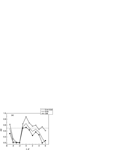
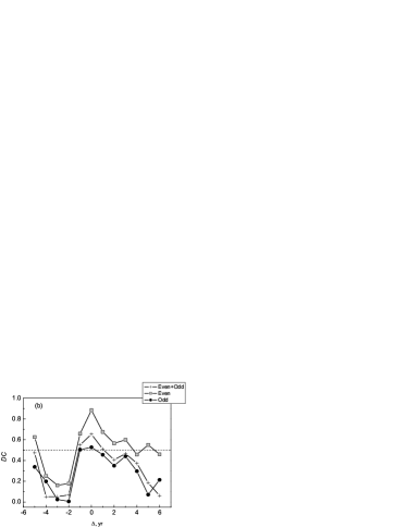
Figure 2: Coefficients of the determination for relations $S\!N_{m-3}$ with $S\!N_{M+\Delta}$ (a) for the linear form (1), (b) for the nonlinear form (2). The parity of the cycles and their mixture corresponds to the legend.

The first thing that can be seen in Figure 2: taking into account the nonlinearity does not lead to a noticeable improvement in correlations. But that’s not the main thing. It turns out that the tightness of the relation $S\!N_{m-3}$ with $S\!N$ in the maximum and the years closest to it strongly depends on the parity of the predicted cycle. We can predict an even cycle with a coefficient of determination D = 0.882 (respectively, with $\rho=0.94$), while an odd cycle — only with $DC=0.524$ ($\rho=0.72$).

According to the prediction in the style of the article by brajsa22, i.e., if we do not take into account the parity of cycles, we get for a maximum of Cycle 25: $S\!N_{M}=129\pm 34$, $\rho=0.808$, which is quite consistent with the values obtained in their article. According to the nonlinear prediction (2), our same values were obtained — taking into account the possible nonlinearity does not give anything additional: $S\!N_{M}=(71\pm 17)+(1.45\pm 0.23)S\!N_{m-3}$. It is also close to the received by brajsa22.

Now let’s see what the regressions and the prediction will look like if we take into account the parity of the cycles. For even cycles regression

$$S\!N_{M}=(50\pm 14)+(1.60\pm 0.18)S\!N_{m-3}\,,\quad\rho=0.939\,,$$ (3)

If our predicted cycle were even, then its maximum would be $S\!N_{M}=113\pm 21$. Confidence intervals due to the high correlation coefficient are very small. However, Cycle 25 is odd. We calculate the regression for odd cycles:

$$S\!N_{M}=(91\pm 29)+(1.32\pm 0.40)S\!N_{m-3}\,,\quad\rho=0.724$$ (4)

and the prediction itself:

$$S\!N_{M}=144\pm 44\,.$$ (5)

This implies that brajsa22, having considered even and odd cycles together, underestimated the predicted value of Cycle 25. The difference in regressions for even and odd cycles is shown in Figure 3a.

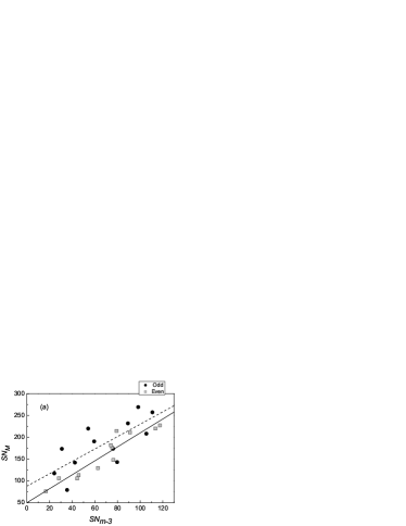
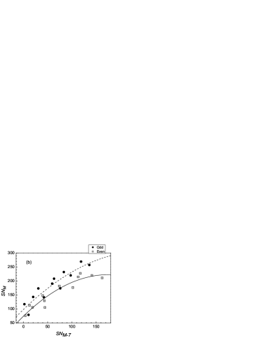
Figure 3: (a) Dependence of $S\!N_{M}$ on $S\!N_{m-3}$ for even (solid line, gray squares) and odd (dashed line, black circles) cycles. (b) Dependence of $S\!N_{M-7}$ on $S\!N$ for even and odd cycles.

Summarizing, according to the effect proposed by brajsa22, we can successfully predict the maximum of the next EVEN cycle three years before the minimum, thereby supplementing the Gnevyshev-Ohl rule with the relation even – subsequent odd cycles. The success of the prediction of an even cycle is guaranteed by a high correlation coefficient of the equation (3).

The precursor of the prediction discussed in this section will be called MI3E for even cycles and MI3O for odd ones (bearing in mind that only MI3E corresponds to a reliable prediction).

4 Cycle precursor associated with the maximum phase

In the paper by slonim84, the idea was expressed to search for cycle precursors a certain number of years before the maximum. Thus, the possible predictors turn out to be associated with the maximum phase, and not with the minimum phase, as in the previous section. Here we will also consider regressions separately for even, odd cycles and for all cycles together, choosing for analysis the same time interval as before, since 1749. Figure 4a illustrates the changes in the coefficients of determination for linear relationships of the type

$$S\!N_{M}=a+b\cdot S\!N_{M+\Delta}\,.$$ (6)

Here we bear in mind that $\Delta=0$ corresponds to the maximum of the cycle. Precursors $S\!N_{M-\Delta}$ correspond to negative $\Delta$ — i.e., years before maximum, positive ones indicate relations with post-maximum years, which are also interesting for the prediction. In addition, we take into account the weak nonlinearity of the relations. For negative $\Delta$ in the form

$$S\!N_{M}=a+b\cdot S\!N_{M+\Delta}+c\cdot S\!N_{M+\Delta}^{2}\,,$$ (7)

and for positive ones —

$$S\!N_{M+\Delta}=a+b\cdot S\!N_{M}+c\cdot S\!N_{M}^{2}\,.$$ (8)

We do this specifically for the possible prediction of not only the maximum values but also the index values in subsequent years, which, as it turns out, are quite closely related to the maximum. The determination coefficients for relations of type (7)–(8) are shown in Figure 4b.

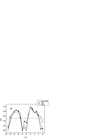
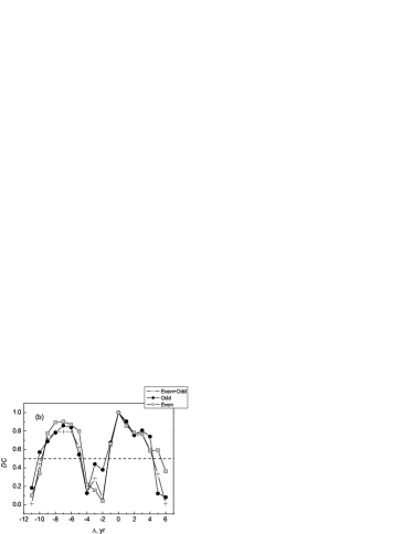
Figure 4: Coefficients of the determination for relations $S\!N_{M}$ with $S\!N_{M+\Delta}$ for (a) linear form (6), (b) nonlinear forms (7)–(8).

Let’s note two circumstances. The first — in comparison with $S\!N_{m-3}$ a more “successful” precursor for the prediction of the maximum is $S\!N_{M-7}$: in the case of a linear form (6) for odd cycles $DC=0.849$ ($\rho=0.921$), for even $DC=0.863$ ($\rho=0.929$); in the case of a nonlinear form (7) for odd $DC=0.859$ ($\rho=0.927$), for even $DC=0.903$ ($\rho=0.950$). Secondly, when considering all cycles together, the correlation of $S\!N_{M-7}$ with $S\!N_{M}$ is less than for each of the parity separately, and this means that their relations are different. This is clearly seen in Figure 3b.

When we predict the amplitude of the future cycle, we are, of course, primarily interested in the amplitude of the maximum, but we are also interested in neighboring years. We found that the predictor of the maximum is $S\!N_{M-7}$. And how much can this value predict the years $M-1$, $M+1$, $M+2$, etc.? Figure 5 answers this question: the seventh year before the maximum is a predictor not only of the maximum but also of the index in the years near the maximum. This applies to both even and odd cycles, although the relations between $S\!N_{M-7}$ and $S\!N_{M+\Delta}$ are different.

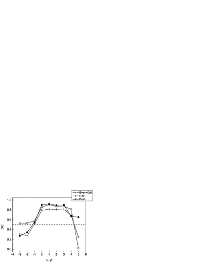
Figure 5: Determination coefficients for quadratic relations of $S\!N_{M-7}$ with $S\!N_{M+\Delta}$.

The prediction precursor discussed in this section we will call MA7E for even cycles and MA7O for odd ones.

Thus, we have created a “constructor” for the prediction of the solar cycle, in this case — the odd solar Cycle 25.

5 Prediction of the solar activity cycle 25

Let’s use the results of the previous sections to predict Cycle 25. We use the MA7O predictor. Assuming different years of maximum onset, we get the $S\!N_{M}$ values given in the Table 2.

Table 2: Predicted $S\!N_{M}$ values depending on the estimated maximum year.

Year	$S\!N_{M}$
2022.5	$199\pm 25$
2023.5	$159\pm 25$
2024.5	$133\pm 25$

Then, using regressions, the coefficients of determination of which are shown in Figure 5, we calculate the values of $S\!N$ in the years of Cycle 25, which have prognostic significance, for different maximum years from Table 2.

The results are shown in Figure 6a: light icons — rhombuses, squares, and circles — connected by a dashed line constructed using a global cubic spline. Comparing the obtained curves with the course of the monthly average values of $S\!N$ observed up to June 2022 (small circles connected by thin lines), we conclude that 2023.5 is the most preferable of the three years of the assumed maximum from Table 2. However, in general, the monthly average values are located, although close to the interpolation curve, but still somewhat below her. Let’s assume a new maximum date — 2024.0. Note that the average annual values can be calculated by averaging $S\!N$ not only traditionally from January to December but also from July to June of the next year, and. Let’s calculate such annual averages, output regressions with determination coefficients similar to those shown in Figure 5, and calculate the values for the dates 2023.0–2028.0 in annual increments — see Figure 6a: black circles connected by a thick spline curve. It can be seen that by assuming a maximum year of 2024.0 we get a better agreement of the behavior of the predicted and observed $S\!N$.

Now about the values indicated in Figure 6a by crosses. Are there any general trends in the last years of the cycle (in our case, the odd one)? Consider the values of $S\!N$ in the years of the final minima of the odd cycle $m$ and the two years before it $m-1$ and $m-2$, depending on their distance from the initial minimum $\Delta$. It turns out that this dependence can be described by a parabola $S\!N(\Delta)=(327\pm 87)-(50\pm 18)\Delta+(1.96\pm 0.87)\Delta^{2}$ with a correlation coefficient $\rho=0.811$, i.e. sufficiently high, and we can use it to predict the descending phase of a new cycle (as it seems, this is a new unexpected result). In Figure 6a crosses represent data given by the date of the initial minimum of Cycle 25 as $2019.5\pm\Delta$. Note here that for even cycles, a similar dependence also occurs, although the correlation coefficient with the parabola is somewhat less — $\rho=0.768$ . However, it can also be used for solar cycle prediction in the future.

So far, for predictions, we have used confidence ranges of estimates for a deviation equal to the standard deviation (i.e., with a probability of falling into the interval equal to 68%) — as in brajsa22, as well as in many authors of solar cycle predictions. In fact, if we want to achieve a reliability of at least 95%, we need to set a prediction interval based on at least two standard deviations. Therefore, we will repeat all the previous procedures for this new requirement. The average annual values of $S\!N$, interpreted for years with traditional calculation from January to December, with confidence bands are shown in Figure 6b.

Note that our methodology allows us to predict individual average annual values of $S\!N$ in a cycle, and not only the amplitude of its maximum, as with most authors.

Having made a prediction of the Cycle 25, it is natural to check whether the Gnevyshev-Ohl rule is fulfilled for a pair of Cycles 24–25. In Figure 1a, the corresponding point is circled. As we can see, our prediction does not contradict this well-known rule.

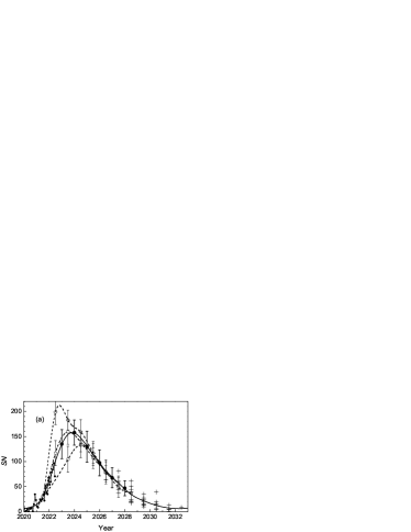
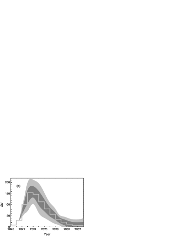
Figure 6: (a) Various versions of predictions for the development of Cycle 25 — see the legend in the text; (b) The most probable prediction of Cycle 25. Light gray areas are the prediction interval with a confidence of 68%, dark gray areas are the same with a confidence of 95%, and a stepped line is the most probable prediction of average annual values.

1

6 Results

The Gnevyshev-Ohl rule establishes a relation between adjacent 11-year cycles in the 22-year “magnetic” Hale cycle as: “an even cycle determines the next odd one,” and thus they form a pair. In this work, we found that the behavior of an odd cycle determines the behavior of the subsequent even one. Namely, 3 years before the minimum, the value of $S\!N$ in the odd cycle is associated with the value of the maximum in the subsequent even cycle (correlation coefficient $\rho=0.94$. Similar to GOR, in this sense, cycles are linked in pairs, but opposite to the Rule. This is one of the important results of the work.

Based on this result, we propose to use $S\!N_{m-3}$ (Figure 3a) as a precursor of the subsequent EVEN cycle during the descending phase of the odd one — we call this method MI3E. For the prediction of an odd cycle or a prediction without parity (as in the article by brajsa22), this method gives less reliable results.

To predict the ODD cycle, we propose to use the precursor of the seventh year to its maximum MA7O — $S\!N_{M-7}$ during the descending phase of the previous even cycle (Figure 3b). It turned out that in this case, we can predict the years near the maximum with a high correlation coefficient ($\rho=0.90{-}0.94$). In addition, 7 years before the maximum, it is also possible to predict an even cycle according to the MA7E precursor (Figure 5).

Also noteworthy is the similar behavior of $S\!N$ for different cycles near the final minimum of the cycle, depending on the distance from the initial minimum. Thus, the proposed approaches make it possible to predict cycles of different parity.

The current Cycle 25 in the year 2023 should reach a maximum of 154 average annual values with a prediction interval of 25 with a confidence of 68% and 53 with a confidence of 95%. This is higher than the original official prediction of NOAA/NASA/ISES but lower than the updated prediction of leamon21 according to the methodology of macint20. In 2024, $S\!N$ will be almost as high as in 2023 — 147 units, so with smaller time averaging scales, the maximum will fall at the end of 2023. Here we note that the proposed approach makes it possible to predict the values of $S\!N$ in individual years of the cycle, and not only the amplitude of its maximum.

We have not discussed in this article the relationship between the precursors $S\!N_{m-3}$ and $S\!N_{M-7}$, their relative position on the descending phase of cycles, as well as their physical meaning — this is the task of the following studies.

Yury Nagovitsyn thanks the Ministry of Science and Higher Education of the Russian Federation for financial support for project 075–15–2020–780.

References

- Brajša et al. (2022) Brajša, R.; Verbanac, G.; Bandić, M.; Hanslmeier, A.; Skokić, I.; Sudar, D.: 2022, Astron. Nachr., 343(3), article id. e13960. DOI: 10.1002/asna.202113960
- Clette et al. (2014) Clette, F.; Svalgaard, L.; Vaquero, J.M.; Cliver, E.W.: 2014, Space Sci. Rev., 186(1-4), 35. DOI: 10.1007/s11214-014-0074-2
- Clette et al. (2016) Clette, F.; Cliver, E.W.; Lefèvre, L.; Svalgaard, L.; Vaquero, J.M.; Leibacher, J.W.: 2016, Solar Phys., 291(9-10), 2479. DOI: 10.1007/s11207-016-1017-8
- Gnevyshev and Ohl (1948) Gnevyshev, M. N.; Ohl, A. I.: 1948, Astron. Zh., 25, 18.
- Leamon et al. (2021) Leamon, R.J., McIntosh, S.W., Chapman, S.C., Watkins, N.W.: 2021, Sol. Phys., v. 296(10), 151. DOI: 10.1007/s11207-021-01897-z
- McIntosh et al. (2020) McIntosh, S.W.; Chapman, Sandra, Leamon, Robert J., Egeland, Ricky, Watkins Nicholas W.: 2020, Solar Phys, 295(12), 163. DOI: 10.1007/s11207-020-01723-y
- Nagovitsyn (2009) Nagovitsyn Yu. A.: 2009, Astron. Lett., , 35(8), 564. DOI: 10.1134/S1063773709080064
- Ohl (1966) Ohl, A. I.: 1966, Byulletin Solnechnye Dannye Akademie Nauk USSR, 12, 84
- Pesnell (2014) Pesnell, W.D.: 2014, Solar Phys. 289(6), 2317. DOI: 10.1007/s11207-013-0470-x
- Petrovay (2020) Petrovay, K.: 2020, Liv. Rev. Sol. Phys., 17(1), 2. DOI: 10.1007/s41116-020-0022-z
- Slonim (1984) Slonim Yu.M. 1984: Byulletin Solnechnye Dannye Akademie Nauk USSR, 5, 78. ADS: https://ui.adsabs.harvard.edu/abs/1984BSolD1984Q..78S/abstract
- Svalgaard el al. (2005) Svalgaard, L.; Cliver, E.W.; Kamide, Y.: 2005, Geophysical Research Letters, 32, L01104.
- Svalgaard and Schatten (2016) Svalgaard, L.; Schatten, K.H.: 2016, Solar Phys., 291(9-10), 2653. DOI: 10.1007/s11207-015-0815-8
- Usoskin et al. (2016) Usoskin, I.G.; Kovaltsov, G.A.; Lockwood, M.; Mursula, K.; Owens, M.; Solanki, S.K.: 2016, Solar Phys., 291(9-10), 2685. DOI: 10.1007/s11207-015-0838-1
- Vitinsky (1973) Vitinsky, Yu.I., Tsiklichnost’ i prognozy solnechnoi aktivnosti (Cyclicity and Forecasting of Solar Activity), Moscow: Nauka, 1973 [in Russian].
- Wilson et al. (1998) Wilson, R. M.; Hathaway, D. H.; Reichmann, E. J.: 1998, Journ. Geophys. Res., 103(A4), 6595. DOI: 10.1029/97JA02777