Measurement of $e^{+}e^{-}\rightarrow\pi^{+}\pi^{-}D^{+}D^{-}$ cross sections at center-of-mass energies from 4.190 to 4.946 GeV

Abstract

Using data samples collected with the BESIII detector operating at the BEPCII storage ring, we measure the cross sections of the $e^{+}e^{-}\rightarrow\pi^{+}\pi^{-}D^{+}D^{-}$ process at center-of-mass energies from 4.190 to 4.946 GeV with a partial reconstruction method. Two resonance structures are seen and the resonance parameters are determined from a fit to the cross section line shape. The first resonance we observe has a mass of (4373.1 $\pm$ 4.0 $\pm$ 2.2) MeV/$c^{2}$ and a width of (146.5 $\pm$ 7.4 $\pm$ 1.3) MeV, in agreement with those of the $Y(4390)$ state; the other resonance has a mass of (4706 $\pm$ 11 $\pm$ 4) MeV/$c^{2}$, a width of (45 $\pm$ 28 $\pm$ 9) MeV, and a statistical significance of $4.1$ standard deviations ($\sigma$). This is the first evidence for a vector state at this mass value. The spin-$3$ $D$-wave charmonium state $X(3842)$ is searched for through the $e^{+}e^{-}\rightarrow\pi^{+}\pi^{-}X(3842)\rightarrow\pi^{+}\pi^{-}D^{+}D^{-}$ process, and evidence with a significance of $4.2\sigma$ is found in the data samples with center-of-mass energies from 4.600 to 4.700 GeV.

I Introduction

The charmonium states with masses below the open charm threshold and a few vector states above the open charm threshold are well-established pdg , and they agree well with theoretical calculations based on QCD Brambilla:2004jw ; review4 ; Brambilla:2014jmp and QCD-inspired potential models eichten ; godfrey ; barnes . The vector charmonia $\psi(4040)$, $\psi(4160)$, and $\psi(4415)$ were assigned as the $3^{3}S_{1}$, $2^{3}D_{1}$, and $4^{3}S_{1}$ states, respectively, since only these three structures were observed in the total $e^{+}e^{-}$ annihilation cross section bes2_psis .

However, a few more vector states, the $Y$ states, were discovered by the BaBar and Belle $B$-factory experiments PBFB . These include the $Y(4260)$ babar_y4260 , the $Y(4360)$ babar_y4360 ; belle_y4660 , and the $Y(4660)$ belle_y4660 . They are produced via the initial state radiation (ISR) process in $e^{+}e^{-}$ annihilation and, thus, are vector states with quantum numbers $J^{PC}=1^{--}$, the same as the excited $\psi$ states listed above. These states were observed in hidden-charm final states in contrast to the excited $\psi$ states peaking in the inclusive hadronic cross section bes2_psis ; uglov-kmatrix . The final states in the latter are dominated by open-charm meson pairs.

In potential models, five vector charmonium states with masses between 4.0 and 4.7 GeV/$c^{2}$ are expected, namely the $\psi(3^{3}S_{1})$, $\psi(2^{3}D_{1})$, $\psi(4^{3}S_{1})$, $\psi(3^{3}D_{1})$, and $\psi(5^{3}S_{1})$. The first three are often identified as the $\psi(4040)$, $\psi(4160)$, and $\psi(4415)$ states, respectively. The masses of the as yet undiscovered $\psi(3D)$ and $\psi(5S)$ are expected to be higher than 4.4 GeV/$c^{2}$. However, six vector states have been identified in the mass region between 4.0 and 4.7 GeV/$c^{2}$, as listed above. This makes the $Y(4260)$, the $Y(4360)$, and perhaps the $Y(4660)$ states good candidates for new types of exotic particles, and has stimulated theoretical work regarding their interpretation. They have been variously considered as candidates for tetraquark states, molecular states, hybrid states, and hadro-charmonia review1 ; review2 ; review3 ; review4 .

With masses above the open-charm thresholds, both $Y$ and excited $\psi$ states should couple to open-charm final states, and many studies have been performed to measure the cross sections of two-body final states with a pair of charmed mesons DD ; 2018DD ; 2020DsstDs1 ; 2021DsstDsj and three-body final states with a pair of charmed mesons and a light meson bes3_ddstarpi . Although four-body final states with a pair of charmed mesons and a pair of light mesons 2019HY ; 2020ZY have also been studied, and the production of intermediate two-body ($D_{1}(2420)\bar{D}+c.c.$) and three-body ($\pi^{+}\pi^{-}\psi(3770)$) states have been observed, the total cross section of the four-body final states has not been reported. In such final states, new exotic particles and new decay modes of known $Y$ and excited $\psi$ states can be searched for.

In this paper, we report the first measurement of the cross sections of the $e^{+}e^{-}\rightarrow\pi^{+}\pi^{-}D^{+}D^{-}$ process with the data samples taken at 37 center-of-mass energies ($\sqrt{s}$) from 4.190 to 4.946 GeV, the study of the decays of the excited $\psi$ and $Y$ states into this final state, and the observation of a new resonant structure in the cross section line shape.

Two of the $D$-wave spin-triplet states $\psi(1^{3}D_{1})$ ($\psi(3770)$) and $\psi(1^{3}D_{2})$ ($\psi_{2}(3823)$) have been observed in the $e^{+}e^{-}$ annihilation process $e^{+}e^{-}\to\pi^{+}\pi^{-}\psi(1D)$ 2019HY ; 2020ZY ; 2015X3823 . As their spin partner, the $\psi(1^{3}D_{3})$ ($X(3842)$) observed by LHCb 2019X3842 can also be produced in a similar process and can be searched for in the $\pi^{+}\pi^{-}D^{+}D^{-}$ final state, since the $X(3842)$ decays to $D\bar{D}$.

II Detector and data samples

The BESIII detector Ablikim:2009aa records $e^{+}e^{-}$ collisions provided by the BEPCII storage ring Yu:IPAC2016-TUYA01 . The cylindrical core of the BESIII detector covers 93% of the full solid angle and consists of a helium-based multilayer drift chamber (MDC), a plastic scintillator time-of-flight system (TOF), and a CsI(Tl) electromagnetic calorimeter (EMC), which are all enclosed in a superconducting solenoidal magnet providing a 1.0 T magnetic field. The solenoid is supported by an octagonal flux-return yoke with resistive plate counter muon identification modules interleaved with steel. The charged-particle momentum resolution at $1~{}{\rm GeV}/c$ is $0.5\%$, and the $dE/dx$ resolution is $6\%$ for electrons from Bhabha scattering. The EMC measures photon energies with a resolution of $2.5\%$ ($5\%$) at $1$ GeV in the barrel (end cap) region. The time resolution in the TOF barrel region is 68 ps, while that in the end cap region is 110 ps. The end cap TOF system was upgraded in 2015 using multi-gap resistive plate chamber technology, providing a time resolution of 60 ps etof .

In this analysis, the experimental data samples used are listed in Table 1. The center-of-mass energy is measured using dimuon events with a precision of 0.8 MeV for data samples with $\sqrt{s}$ smaller than 4.610 GeV 2016mumu ; 2021mumu and using $\Lambda_{c}^{+}\bar{\Lambda}_{c}^{-}$ events with a precision of 0.6 MeV for data samples with $\sqrt{s}$ larger than or equal to 4.610 GeV 2022LcLc . The integrated luminosity is determined by analyzing large angle Bhabha scattering events with an uncertainty of 1.0% 2019SWM ; 2022lum ; 2022LcLc . The integrated luminosity of the total data sample is $17.4~{}\rm{fb}^{-1}$.

Table 1: Yields and cross sections results for the $e^{+}e^{-}\rightarrow\pi^{+}\pi^{-}D^{+}D^{-}$ process at different center-of-mass energies. Here, $\sigma$ is the cross section of the $e^{+}e^{-}\rightarrow\pi^{+}\pi^{-}D^{+}D^{-}$ process, where the first uncertainties are statistical and the second systematic; $\mathscr{L}$, $S$, and $\sigma_{\rm ul}$ are the integrated luminosity, statistical significance, and upper limit of the cross section at 90% confidence level, respectively. $N_{\rm signal}$ and $N_{\rm sideband}$ are the number of $e^{+}e^{-}\rightarrow\pi^{+}\pi^{-}D^{+}D^{-}$ events from fits to $RM(D^{+}\pi_{d}^{+}\pi_{d}^{-})$ distributions in $M(K^{-}\pi^{+}\pi^{+})$ signal and sideband regions, respectively.

$\sqrt{s}$ nominal value (GeV)	$\sqrt{s}$ (MeV)	$\mathscr{L}$ ($\rm{pb}^{-1}$)	$N_{\rm{signal}}$		$N_{\rm{sideband}}$		$\sigma\ (\rm{pb})$			$S$	$\sigma_{\rm{ul}}$ (pb)
4.190	$4188.59\pm 0.15\pm 0.68$	570.0	$-$8$\ \pm\$	10	$-$17$\ \pm\$	11	0.1$\ \pm\$	0.9 $\ \pm\$	0.0	-	1.0
4.200	$4199.15\pm 0.05\pm 0.34$	526.0	$-$5$\ \pm\$	11	$-$15$\ \pm\$	12	0.2$\ \pm\$	1.0 $\ \pm\$	0.0	-	1.2
4.210	$4207.73\pm 0.14\pm 0.61$	572.1	15$\ \pm\$	13	19$\ \pm\$	14	0.3$\ \pm\$	1.0 $\ \pm\$	0.1	$\ \ \ 1.2\sigma$	2.6
4.220	$4217.13\pm 0.14\pm 0.67$	569.2	17$\ \pm\$	12	14$\ \pm\$	13	0.7$\ \pm\$	0.9 $\ \pm\$	0.1	$\ \ \ 1.5\sigma$	2.6
4.230	$4225.54\pm 0.05\pm 0.65$	1100.9	119$\ \pm\$	25	12$\ \pm\$	20	3.4$\ \pm\$	0.8 $\ \pm\$	0.3	$\ \ \ 5.9\sigma$	-
4.237	$4235.77\pm 0.04\pm 0.30$	530.3	25$\ \pm\$	14	$-$29$\ \pm\$	13	2.6$\ \pm\$	1.0 $\ \pm\$	0.2	$\ \ \ 1.9\sigma$	3.5
4.245	$4241.66\pm 0.12\pm 0.73$	55.9	5$\ \pm\$	6	$-$3$\ \pm\$	4	4.0$\ \pm\$	3.7 $\ \pm\$	0.3	$\ \ \ 0.9\sigma$	9.0
4.246	$4243.97\pm 0.04\pm 0.30$	538.1	101$\ \pm\$	19	1$\ \pm\$	15	6.1$\ \pm\$	1.3 $\ \pm\$	0.7	$\ \ \ 6.6\sigma$	-
4.260	$4258.00\pm 0.06\pm 0.60$	825.7	159$\ \pm\$	26	17$\ \pm\$	22	5.6$\ \pm\$	1.1 $\ \pm\$	0.5	$\ \ \ 7.5\sigma$	-
4.270	$4266.81\pm 0.04\pm 0.32$	531.1	61$\ \pm\$	18	$-$27$\ \pm\$	17	4.3$\ \pm\$	1.2 $\ \pm\$	0.4	$\ \ \ 3.6\sigma$	6.7
4.280	$4277.78\pm 0.11\pm 0.52$	175.7	25$\ \pm\$	12	2$\ \pm\$	11	4.2$\ \pm\$	2.4 $\ \pm\$	0.4	$\ \ \ 2.2\sigma$	9.0
4.290	$4288.43\pm 0.06\pm 0.34$	502.4	140$\ \pm\$	23	4$\ \pm\$	20	8.6$\ \pm\$	1.6 $\ \pm\$	0.7	$\ \ \ 7.1\sigma$	-
4.310	$4307.89\pm 0.17\pm 0.63$	45.1	25$\ \pm\$	8	$-$4$\ \pm\$	7	17.1$\ \pm\$	5.5 $\ \pm\$	1.5	$\ \ \ 3.4\sigma$	30
4.315	$4312.68\pm 0.06\pm 0.35$	501.2	263$\ \pm\$	29	9$\ \pm\$	23	15.4$\ \pm\$	1.9 $\ \pm\$	1.3	$\ \ \ \ 11\sigma$	-
4.340	$4337.93\pm 0.06\pm 0.35$	505.0	666$\ \pm\$	42	20$\ \pm\$	27	36.9$\ \pm\$	2.5 $\ \pm\$	3.1	$\ \ \ \ \ 21\sigma$	-
4.360	$4358.26\pm 0.05\pm 0.62$	544.0	1038$\ \pm\$	53	8$\ \pm\$	34	48.2$\ \pm\$	2.6 $\ \pm\$	4.1	$\ \ \ \ \ 26\sigma$	-
4.380	$4377.88\pm 0.06\pm 0.35$	522.7	1184$\ \pm\$	67	$-$35$\ \pm\$	37	61.6$\ \pm\$	3.6 $\ \pm\$	5.2	$\ \ \ \ \ 25\sigma$	-
4.390	$4387.40\pm 0.17\pm 0.65$	55.6	111$\ \pm\$	18	19$\ \pm\$	13	46.2$\ \pm\$	8.8 $\ \pm\$	3.9	$\ \ \ 7.4\sigma$	-
4.400	$4396.83\pm 0.06\pm 0.36$	507.8	1217$\ \pm\$	62	61$\ \pm\$	43	61.9$\ \pm\$	3.5 $\ \pm\$	5.2	$\ \ \ \ \ 24\sigma$	-
4.420	$4415.94\pm 0.04\pm 0.62$	1090.7	3144$\ \pm\$	112	216$\ \pm\$	71	67.7$\ \pm\$	2.6 $\ \pm\$	5.8	$\ \ \ \ \ 37\sigma$	-
4.440	$4437.59\pm 0.06\pm 0.35$	569.9	1588$\ \pm\$	85	140$\ \pm\$	59	65.1$\ \pm\$	3.9 $\ \pm\$	5.9	$\ \ \ \ \ 23\sigma$	-
4.470	$4467.06\pm 0.11\pm 0.73$	111.1	192$\ \pm\$	35	36$\ \pm\$	25	36.0$\ \pm\$	7.8 $\ \pm\$	3.9	$\ \ \ 6.8\sigma$	-
4.530	$4527.14\pm 0.11\pm 0.72$	112.1	141$\ \pm\$	34	17$\ \pm\$	28	30.4$\ \pm\$	8.6 $\ \pm\$	3.1	$\ \ \ 4.1\sigma$	41
4.575	$4574.50\pm 0.18\pm 0.70$	48.9	39$\ \pm\$	18	12$\ \pm\$	19	15.5$\ \pm\$	9.9 $\ \pm\$	1.4	$\ \ \ 2.2\sigma$	38
4.600	$4599.53\pm 0.07\pm 0.74$	586.9	811$\ \pm\$	74	$-$16$\ \pm\$	69	31.2$\ \pm\$	3.1 $\ \pm\$	2.8	$\ \ \ \ \ 12\sigma$	-
4.612	$4611.86\pm 0.12\pm 0.32$	103.8	139$\ \pm\$	31	42$\ \pm\$	29	27.3$\ \pm\$	8.1 $\ \pm\$	2.3	$\ \ \ 4.9\sigma$	40
4.620	$4628.00\pm 0.06\pm 0.32$	521.5	758$\ \pm\$	90	30$\ \pm\$	72	33.7$\ \pm\$	4.4 $\ \pm\$	2.9	$\ \ \ \ \ 11\sigma$	-
4.640	$4640.91\pm 0.06\pm 0.38$	552.4	725$\ \pm\$	85	$-$65$\ \pm\$	71	32.2$\ \pm\$	3.9 $\ \pm\$	2.8	$\ \ \ \ \ 10\sigma$	-
4.660	$4661.24\pm 0.06\pm 0.29$	529.6	814$\ \pm\$	93	$-$51$\ \pm\$	73	38.1$\ \pm\$	4.6 $\ \pm\$	3.4	$\ \ \ \ \ 11\sigma$	-
4.680	$4681.92\pm 0.08\pm 0.29$	1669.3	2427$\ \pm\$	156	$-$12$\ \pm\$	128	33.7$\ \pm\$	2.3 $\ \pm\$	2.8	$\ \ \ \ \ 19\sigma$	-
4.700	$4698.82\pm 0.10\pm 0.39$	536.5	1020$\ \pm\$	85	$-$58$\ \pm\$	76	45.7$\ \pm\$	4.1 $\ \pm\$	4.0	$\ \ \ \ \ 13\sigma$	-
4.740	$4739.70\pm 0.20\pm 0.30$	164.3	330$\ \pm\$	45	47$\ \pm\$	41	39.8$\ \pm\$	6.5 $\ \pm\$	3.4	$\ \ \ 8.2\sigma$	-
4.750	$4750.05\pm 0.12\pm 0.29$	367.2	781$\ \pm\$	71	71$\ \pm\$	59	43.2$\ \pm\$	4.5 $\ \pm\$	3.8	$\ \ \ \ \ 13\sigma$	-
4.780	$4780.54\pm 0.12\pm 0.33$	512.8	1042$\ \pm\$	94	217$\ \pm\$	78	39.6$\ \pm\$	4.3 $\ \pm\$	3.3	$\ \ \ \ \ 14\sigma$	-
4.840	$4843.07\pm 0.20\pm 0.31$	527.3	1050$\ \pm\$	100	10$\ \pm\$	81	43.4$\ \pm\$	4.5 $\ \pm\$	3.7	$\ \ \ \ \ 13\sigma$	-
4.914	$4918.02\pm 0.34\pm 0.35$	208.1	471$\ \pm\$	67	40$\ \pm\$	58	48.6$\ \pm\$	7.9 $\ \pm\$	4.2	$\ \ \ 8.2\sigma$	-
4.946	$4950.93\pm 0.36\pm 0.44$	160.4	247$\ \pm\$	51	80$\ \pm\$	51	29.4$\ \pm\$	8.2 $\ \pm\$	2.5	$\ \ \ 5.0\sigma$	-

To increase signal yields, a partial reconstruction method is employed for the $e^{+}e^{-}\rightarrow\pi^{+}\pi^{-}D^{+}D^{-}$ process. A $D^{+}$ meson is reconstructed via its high branching fraction (9.38%) decay mode, $D^{+}\rightarrow K^{-}\pi^{+}\pi^{+}$, and an additional $\pi^{+}\pi^{-}$ pair is selected from the remaining charged tracks. The recoil mass of the $\pi^{+}\pi^{-}D^{+}$ system is used to identify the $D^{-}$ meson. Unless explicitly mentioned, the inclusion of charge conjugate modes is implied throughout the context.

Simulated data samples produced with a geant4-based geant4 Monte Carlo (MC) package, which includes the geometric description of the BESIII detector and the detector response, are used to determine detection efficiencies and to estimate backgrounds. The simulation models the beam energy spread and ISR in the $e^{+}e^{-}$ annihilations with the generator kkmc kkmc .

In order to estimate the potential background contributions, inclusive MC samples generated at $\sqrt{s}=$ 4.230, 4.360, 4.420, and 4.600 GeV are used. The inclusive MC sample includes the production of open charm processes, the ISR production of vector charmonium(-like) states, and the continuum processes incorporated in kkmc kkmc . The known decay modes are modelled with evtgen evtgen using branching fractions taken from the Particle Data Group (PDG) pdg , and the remaining unknown charmonium decays are modelled with lundcharm lundcharm . Final state radiation (FSR) from charged final state particles is incorporated using the photos package photos .

For the optimization of the selection criteria and signal extraction, the following MC samples are produced at each $\sqrt{s}$: $e^{+}e^{-}\rightarrow D_{1}(2420)^{+}D^{-}$, with $D_{1}(2420)^{+}\rightarrow D^{+}\pi^{+}\pi^{-}$, $e^{+}e^{-}\rightarrow\pi^{+}\pi^{-}\psi(3770)$, with $\psi(3770)\rightarrow D^{+}D^{-}$, where $D_{1}(2420)^{+}D^{-}$ and $\pi^{+}\pi^{-}\psi(3770)$ are uniformly distributed in the phase space, and $e^{+}e^{-}\rightarrow\pi^{+}\pi^{-}D^{+}D^{-}(\rm{PHSP})$ where the $\pi^{+}\pi^{-}D^{+}D^{-}$ events are uniformly distributed in the phase space to represent the processes with unknown intermediate states. For the $D_{1}(2420)^{+}\rightarrow D^{+}\pi^{+}\pi^{-}$ process, the $D^{+}\pi^{+}\pi^{-}$ events are also uniformly distributed in the phase space.

III Event Selection

Charged tracks detected in the MDC are required to be within a polar angle ($\theta$) range of $|\cos\theta|<0.93$, where $\theta$ is defined with respect to the z-axis, which is the symmetry axis of the MDC. For charged tracks not originating from $K_{S}^{0}$ or $\Lambda$ decays, the distance of closest approach to the interaction point (IP) must be less than 10 cm along the $z$-axis, $|V_{z}|$, and less than 1 cm in the transverse plane, $|V_{xy}|$. A charged track should have a good quality in the track fitting and be within the angle coverage of the MDC, $|\cos\theta|<0.93$. A good charged track (excluding those from $K_{S}^{0}$ or $\Lambda$ decays) is required to be within 1 cm of the $e^{+}e^{-}$ annihilation interaction point (IP) transverse to the beam line ($|V_{xy}|<1$ cm) and within 10 cm of the IP along the beam axis ($|V_{z}|<10$ cm).

Particle identification (PID) for charged tracks combines measurements of the energy deposited in the MDC (d$E$/d$x$) and the flight time in the TOF to form likelihoods $\mathcal{L}(h)~{}(h=p,K,\pi)$ for each hadron $h$ hypothesis. Tracks are identified as protons when the proton hypothesis has the greatest likelihood ($\mathcal{L}(p)>\mathcal{L}(K)$ and $\mathcal{L}(p)>\mathcal{L}(\pi)$), while charged kaons and pions are identified by comparing the likelihoods for the kaon and pion hypotheses, $\mathcal{L}(K)>\mathcal{L}(\pi)$ and $\mathcal{L}(\pi)>\mathcal{L}(K)$, respectively.

Particle identification (PID) for charged tracks combines measurements of the energy loss in the MDC ($dE/dx$) and the flight time in the TOF. Likelihoods $\mathcal{L}(h)$ ($h=K$, $\pi$, $p$) for each hadron $h$ hypothesis are formed and each track is assigned to the particle type corresponding to the hypothesis with the greatest likelihood. A proton (or an anti-proton) is identified if $\mathcal{L}(p)>\mathcal{L}(\pi)$ and $\mathcal{L}(p)>\mathcal{L}(K)$. In order to suppress background from $e^{+}e^{-}\rightarrow\Lambda_{c}^{+}\bar{\Lambda}_{c}^{-}$ and other possible charmed baryons, events with proton or anti-proton tracks are rejected. Charged kaons and pions are identified by comparing the likelihoods for the kaon and pion hypotheses, $\mathcal{L}(K)>\mathcal{L}(\pi)$ and $\mathcal{L}(\pi)>\mathcal{L}(K)$, respectively.

To reconstruct the $D^{+}$ meson, one $K^{-}$ and two $\pi^{+}$ candidate tracks are selected. They are required to originate from a common vertex and the quality of the vertex fit is required to satisfy $\chi^{2}_{VF}<100$. All possible $K^{-}\pi^{+}\pi^{+}$ combinations in the event which satisfy these criteria are kept as $D^{+}$ candidates for further analysis. There are 1.1 $D^{+}$ candidates per event on average after $M(K^{-}\pi^{+}\pi^{+})$ and $RM(D^{+}\pi_{d}^{+}\pi_{d}^{-})$ requirements mentioned in the following paragraph. For each $D^{+}$ candidate, a $\pi^{+}\pi^{-}$ pair is selected from the charged tracks not used in $D^{+}$ reconstruction (referred to as $\pi_{d}^{+}$ and $\pi_{d}^{-}$) and the recoil mass of $D^{+}\pi_{d}^{+}\pi_{d}^{-}$ ($RM(D^{+}\pi_{d}^{+}\pi_{d}^{-})$) is calculated to identify the $D^{-}$ candidate.

Figure 1 shows $RM(D^{+}\pi_{d}^{+}\pi_{d}^{-})$ versus the invariant mass of the $K^{-}\pi^{+}\pi^{+}$ ($M(K^{-}\pi^{+}\pi^{+})$) for data samples at $\sqrt{s}=$ 4.230, 4.420, and 4.680 GeV. Clear $D^{-}$ and $D^{+}$ signal peaks can be seen in the $RM(D^{+}\pi_{d}^{+}\pi_{d}^{-})$ and $M(K^{-}\pi^{+}\pi^{+})$ distributions, respectively. The $\pi^{+}\pi^{-}D^{+}D^{-}$ signal region is defined as $|M(K^{-}\pi^{+}\pi^{+})-m_{D^{+}}|<d_{M}$ and $|RM(D^{+}\pi_{d}^{+}\pi_{d}^{-})-m_{D^{-}}|<d_{RM}$, and the sideband regions as $-5d_{M}<M(K^{-}\pi^{+}\pi^{+})-m_{D^{+}}<-3d_{M}$ or $3d_{M}<M(K^{-}\pi^{+}\pi^{+})-m_{D^{+}}<5d_{M}$ , and $-5d_{RM}<RM(D^{+}\pi_{d}^{+}\pi_{d}^{-})-m_{D^{-}}<-3d_{RM}$ or $3d_{RM}<RM(D^{+}\pi_{d}^{+}\pi_{d}^{-})-m_{D^{-}}<5d_{RM}$ , where $m_{D^{\pm}}=1.86966$ GeV/$c^{2}$ is the known $D^{\pm}$ mass pdg . The signal and sideband regions are indicated in Fig. 1. A linear mass or recoil mass dependence is assumed in estimating the background level in the signal region. The widths of the window are $d_{M}=11$ MeV/$c^{2}$ for all the data samples, and $d_{RM}=6$ MeV/$c^{2}$ for data samples with $\sqrt{s}$ smaller than 4.310 GeV, and $d_{RM}=9$ MeV/$c^{2}$ for data samples with $\sqrt{s}$ greater than or equal to 4.310 GeV. Each sideband has the same width as that of the signal region.

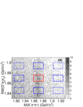
Figure 1: Distributions of $RM(D^{+}\pi_{d}^{+}\pi_{d}^{-})$ versus $M(K^{-}\pi^{+}\pi^{+})$ for data samples at $\sqrt{s}$ = 4.230 (a), 4.420 (b), and 4.680 (c) GeV. The red solid box shows the signal region, the blue dashed boxes the sideband regions with one real $D^{+}$ or $D^{-}$ candidate, and the blue dotted boxes the sideband regions with fake $D^{+}$ and $D^{-}$ candidates. The indices of the boxes from top to bottom and left to right are ($-$1, 1), (0, 1), (1, 1), ($-$1, 0), (0, 0), (1, 0), ($-$1, $-$1), (0, $-$1), and (1, $-$1), respectively. The region with index (0, 0) is the signal region, while the others are the sideband regions (color version online).

After requiring $|RM(D^{+}\pi_{d}^{+}\pi_{d}^{-})-m_{D^{-}}|<d_{RM}$, the $M(K^{-}\pi^{+}\pi^{+})$ distributions are shown in Fig. 2 for data samples at $\sqrt{s}=$ 4.230, 4.420, and 4.680 GeV as examples. In the following analysis, the $K^{-}\pi^{+}\pi^{+}$ combination in the signal region is constrained to the known $D^{+}$ mass, $m_{D^{+}}$, with a kinematic fit to improve its momentum resolution, and those in the sideband regions are constrained to the central value of the corresponding sideband region.

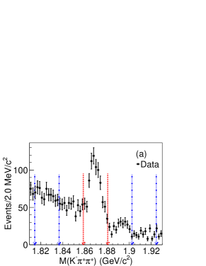
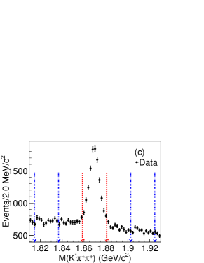
Figure 2: The $K^{-}\pi^{+}\pi^{+}$ invariant mass distributions for data samples at $\sqrt{s}=$ 4.230 (a), 4.420 (b), and 4.680 (c) GeV. The black dots with error bars are data, the regions between the two red dashed arrows are $D^{+}$ signal regions and those between blue dash-dotted arrows are sideband regions (color version online).

Figure 3 shows the $RM(D^{+}\pi_{d}^{+}\pi_{d}^{-})$ distributions after requiring $|M(K^{-}\pi^{+}\pi^{+})-m_{D^{+}}|<d_{M}$ for data samples at $\sqrt{s}=$ 4.230, 4.420, and 4.680 GeV. Clear $D^{-}$ signal peaks are visible in all data samples. The $D^{-}$ signal and sideband regions are indicated by the arrows.

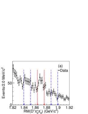
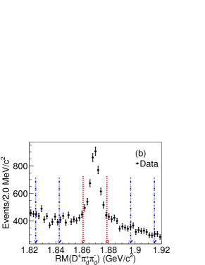
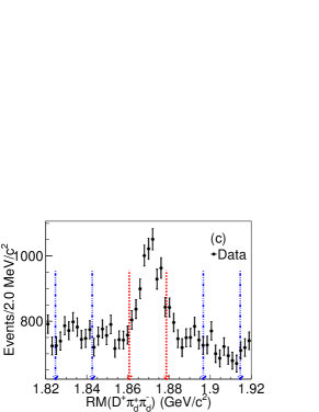
Figure 3: Distributions of $RM(D^{+}\pi_{d}^{+}\pi_{d}^{-})$ in the $M(K^{-}\pi^{+}\pi^{+})$ signal region for data samples at $\sqrt{s}=$ 4.230 (a), 4.420 (b), and 4.680 (c) GeV. The black dots with error bars are data, the regions between the two red dashed arrows are $D^{-}$ signal regions and those between blue dash-dotted arrows are sideband regions (color version online).

The $e^{+}e^{-}\rightarrow D^{0}D^{-}\pi^{+}$ process produces a peaking background in the $RM(D^{+}\pi_{d}^{+}\pi_{d}^{-})$ distribution as shown in Fig. 4(a). The peaking background may come from $e^{+}e^{-}\rightarrow D^{0}D^{-}\pi^{+}$, with $D^{0}\rightarrow K^{-}\pi_{d}^{+}\pi_{d}^{-}\pi^{+}$, where a directly produced $\pi^{+}$, together with $\pi^{+}$ and $K^{-}$ from $D^{0}$, forms the tagged $D^{+}$. Figure 4(b) shows the $M(K^{-}\pi_{d}^{+}\pi_{d}^{-}\pi^{+})$ distribution, where a clear $D^{0}$ peak is seen. We require $|M(K^{-}\pi_{d}^{+}\pi_{d}^{-}\pi^{+})-m_{D^{0}}|>0.01$ GeV/$c^{2}$ to veto these $D^{0}$ background contributions, where $m_{D^{0}}=$ 1.86484 GeV/$c^{2}$ pdg . The value of $0.01$ GeV/$c^{2}$ corresponds to twice the resolution of $M(K^{-}\pi_{d}^{+}\pi_{d}^{-}\pi^{+})$, which is 0.0045 GeV/$c^{2}$. The effectiveness of this veto can be seen in Fig. 4(c). The number of $e^{+}e^{-}\rightarrow\pi^{+}\pi^{-}D^{+}D^{-}$ events from fits to the $RM(D^{+}\pi_{d}^{+}\pi_{d}^{-})$ distributions in the $M(K^{-}\pi^{+}\pi^{+})$ sideband region before and after the veto are 614 $\pm$ 92 and 216 $\pm$ 72, respectively.

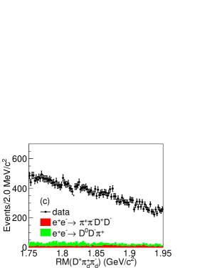
Figure 4: The $RM(D^{+}\pi_{d}^{+}\pi_{d}^{-})$ distribution for combinations in the $M(K^{-}\pi^{+}\pi^{+})$ sideband before (a) and after (c) the $D^{0}$ veto at $\sqrt{s}=$ 4.420 GeV. The $M(K^{-}\pi_{d}^{+}\pi_{d}^{-}\pi^{+})$ distribution in the $M(K^{-}\pi^{+}\pi^{+})$ signal region is shown in the middle plot (b). The black dots with error bars are data and the red and green histograms are MC simulations of $e^{+}e^{-}\rightarrow\pi^{+}\pi^{-}D^{+}D^{-}(\rm{PHSP})$ and $e^{+}e^{-}\rightarrow D^{0}D^{-}\pi^{+}$ processes, respectively, with inclusive decays of both $D$ mesons (color version online). The normalizations of $e^{+}e^{-}\rightarrow\pi^{+}\pi^{-}D^{+}D^{-}(\rm{PHSP})$ and $e^{+}e^{-}\rightarrow D^{0}D^{-}\pi^{+}$ processes are accroding to cross sections of total $e^{+}e^{-}\rightarrow\pi^{+}\pi^{-}D^{+}D^{-}$ process and $e^{+}e^{-}\rightarrow D^{0}D^{-}\pi^{+}$ process measured from data samples, respectively.

After applying all the above selection criteria, we compare distributions for events in the $D^{+}$ and $D^{-}$ signal region ($S$ sample) and sideband regions ($B$ sample) to further suppress non-$\pi^{+}\pi^{-}D^{+}D^{-}$ background. The $B$ sample is defined as

$$\begin{split}B=f_{1}\cdot(B_{-1,0}+B_{1,0})+f_{2}\cdot(B_{0,-1}+B_{0,1})-\\ f_{3}\cdot(B_{-1,-1}+B_{1,-1}+B_{-1,1}+B_{1,1}),\end{split}$$ (1)

where $B_{i,j}$ is the sideband region defined in Fig. 1, $f_{1}=0.5$, $f_{2}=0.5$, and $f_{3}=f_{1}f_{2}=0.25$ are the normalization factors assuming a linear mass dependence in the background distributions. In order to improve the momentum resolutions of the final state particles, $D^{+}$ and $D^{-}$ mass constraints and a total four-momentum conservation constraint to that of the initial $e^{+}e^{-}$ system are applied. For events in the $D^{+}$ or $D^{-}$ sidebands, the masses of the $D^{+}$ and $D^{-}$ combinations are constrained to the central values of the corresponding sideband region.

The invariant mass distribution of the $\pi_{d}^{+}\pi_{d}^{-}$ pair is shown in Fig. 5(a), where clear $K_{S}^{0}$ peaks can be seen in both the $S$ and $B$ samples. In order to veto the $K_{S}^{0}\rightarrow\pi_{d}^{+}\pi_{d}^{-}$ background, a secondary vertex fit is performed on the $\pi_{d}^{+}\pi_{d}^{-}$ pair. The decay length $L_{\pi_{d}^{+}\pi_{d}^{-}}$ divided by its uncertainty $\Delta_{L_{\pi_{d}^{+}\pi_{d}^{-}}}$ of the combinations with $\pi_{d}^{+}\pi_{d}^{-}$ invariant mass between 491.0 and 503.5 MeV/$c^{2}$ is shown in Fig. 5(b). By requiring $|L_{\pi_{d}^{+}\pi_{d}^{-}}/\Delta_{L_{\pi_{d}^{+}\pi_{d}^{-}}}|<2$ the $K_{S}^{0}$ background is suppressed significantly as shown in Fig. 5(c).

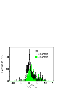
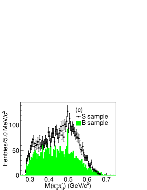
Figure 5: Distributions of $M(\pi_{d}^{+}\pi_{d}^{-})$ before (a) and after (c) the $|L_{\pi_{d}^{+}\pi_{d}^{-}}/\Delta_{L_{\pi_{d}^{+}\pi_{d}^{-}}}|<2$ requirement, and the $L_{\pi_{d}^{+}\pi_{d}^{-}}/\Delta_{L_{\pi_{d}^{+}\pi_{d}^{-}}}$ distribution (b) at $\sqrt{s}=$ 4.420 GeV. The black dots with error bars stand for the $S$ sample and the green shaded histograms for the $B$ sample (color version online).

The $|V_{xy}|$ and $|V_{z}|$ distributions of the $K^{-}$ and $\pi^{+}$ tracks used in $D^{+}$ tag, and the $\pi_{d}^{+}$ and $\pi_{d}^{-}$ tracks from direct $e^{+}e^{-}$ annihilation are shown in Fig. 6. Compared with the typical requirements of less than 1 cm and 10 cm for $|V_{xy}|$ and $|V_{z}|$, respectively, a set of tighter selection criteria $|V_{xy}|<0.55$ cm and $|V_{z}|<3$ cm is identified by optimizing the $\pi^{+}\pi^{-}D^{+}D^{-}$ signal significance.

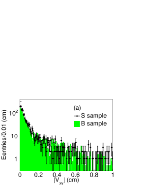
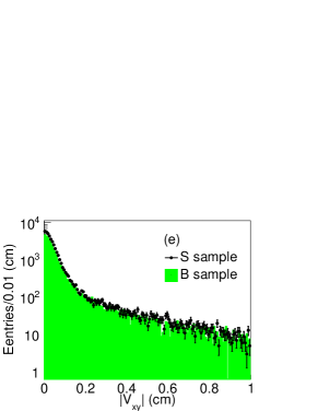
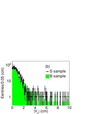
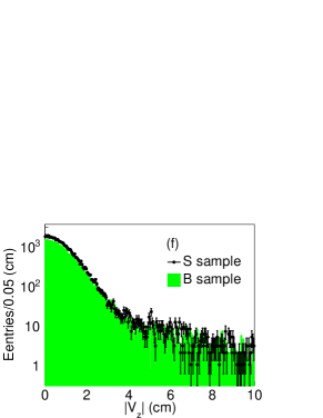
Figure 6: Distributions of $|V_{xy}|$ for data samples at $\sqrt{s}=$ 4.230 (a), 4.420 (c), and 4.680 (e) GeV, and those of $|V_{z}|$ for data samples at $\sqrt{s}=$ 4.230 (b), 4.420 (d), and 4.680 (f) GeV. The black dots with error bars correspond to the $S$ sample and the shaded histograms to the $B$ sample (color version online).

After applying all the above selection criteria, requiring $|M(K^{-}\pi^{+}\pi^{+})-m_{D^{+}}|<d_{M}$, and constraining $M(K^{-}\pi^{+}\pi^{+})$ to the $D^{+}$ mass, we obtain the $RM(D^{+}\pi_{d}^{+}\pi_{d}^{-})$ distributions (Figs. 7(a, c, e)) for data samples at $\sqrt{s}=$ 4.230, 4.420, and 4.680 GeV. Clear $D^{-}$ signal peaks are observed in all these data samples. The non-$\pi^{+}\pi^{-}D^{+}D^{-}$ background is studied by examining the $RM(D^{+}\pi_{d}^{+}\pi_{d}^{-})$ distributions (Figs. 7(b, d, f)) for $K^{-}\pi^{+}\pi^{+}$ combinations in the $D^{+}$ mass sideband regions, defined as $-5d_{M}<M(K^{-}\pi^{+}\pi^{+})-m_{D^{+}}<-3d_{M}$ or $3d_{M}<M(K^{-}\pi^{+}\pi^{+})-m_{D^{+}}<5d_{M}$. No significant $D^{-}$ signal peaks are observed in the sideband samples. In calculating $RM(D^{+}\pi_{d}^{+}\pi_{d}^{-})$ for the sideband events, the $M(K^{-}\pi^{+}\pi^{+})$ is constrained to the central values of the corresponding sideband region rather than to the known mass $m_{D^{+}}$. The number of $e^{+}e^{-}\to\pi^{+}\pi^{-}D^{+}D^{-}$ signal events is obtained by subtracting the number of $D^{-}$ signal candidates in the $D^{+}$ sideband regions from that in the $D^{+}$ signal region, as discussed in Sec. IV.

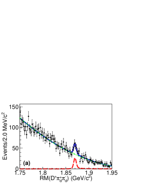
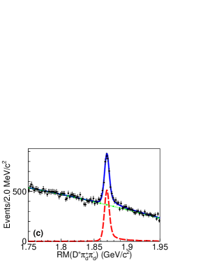
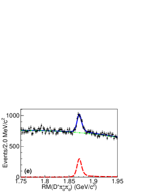
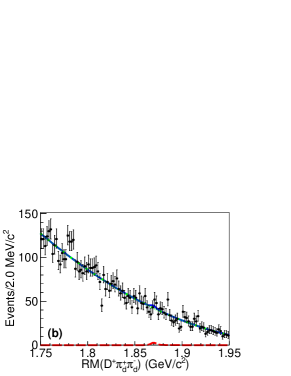
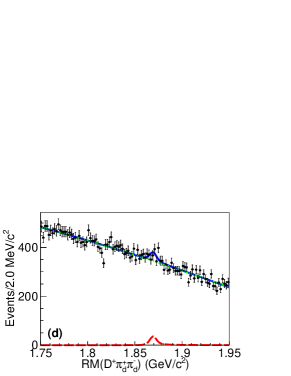
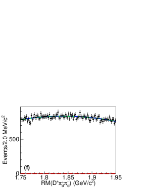
Figure 7: Distributions of $RM(D^{+}\pi_{d}^{+}\pi_{d}^{-})$ in $M(K^{-}\pi^{+}\pi^{+})$ signal (a, c, e) and sideband (b, d, f) regions for data samples at $\sqrt{s}=$ 4.230 (a, b), 4.420 (c, d), and 4.680 (e, f) GeV, and the best fits to the distributions. The black dots with error bars are data, the red dashed, green dash-dotted, and blue solid lines are the signal, background, and total fit, respectively (color version online). The fit qualities are tested using a $\chi^{2}$-test method, with $\chi^{2}/\rm{n.\ d.\ f.}=$93.72/91, 96.39/95, 83.74/93, 104.25/95, 98.69/93, and 85.12/95 for (a), (b), (c), (d), (e), and (f), respectively.

IV Cross sections of the $e^{+}e^{-}\rightarrow\pi^{+}\pi^{-}D^{+}D^{-}$ process

The cross section of the $e^{+}e^{-}\rightarrow\pi^{+}\pi^{-}D^{+}D^{-}$ process is calculated with

$$\sigma=\frac{N_{\rm signal}-N_{\rm sideband}/2}{2f(\sum_{i}\omega_{i}\epsilon_{i}(1+\delta)_{i})\frac{1}{|1-\Pi|^{2}}\mathscr{B}\mathscr{L}},$$ (2)

where $N_{\rm signal}$ and $N_{\rm sideband}$ are the number of $e^{+}e^{-}\rightarrow\pi^{+}\pi^{-}D^{+}D^{-}$ events from fits to $RM(D^{+}\pi_{d}^{+}\pi_{d}^{-})$ distributions (Fig. 7) in the $M(K^{-}\pi^{+}\pi^{+})$ signal and sideband regions, respectively, $\frac{1}{|1-\Pi|^{2}}$ is the vacuum polarization factor, $\mathscr{B}$ is the branching fraction of the decay $D^{+}\rightarrow K^{-}\pi^{+}\pi^{+}$ pdg , and $\mathscr{L}$ is the integrated luminosity of the data sample. $f$ denotes an efficiency correction factor

$$\begin{split}f=f^{M(K^{-}\pi^{+}\pi^{+})}f^{K\nrightarrow p}f^{V_{xy,\ z}}f^{L/\Delta_{L}}\\ f^{RM(D^{+}\pi_{d}^{+}\pi_{d}^{-})},\end{split}$$ (3)

with $f^{v}$ referring to the efficiency correction factor caused by selection criterion $v$, which includes $M(K^{-}\pi^{+}\pi^{+})$ and $RM(D^{+}\pi_{d}^{+}\pi_{d}^{-})$ mass window requirements, $p/\bar{p}$ veto ($K\nrightarrow p$), $V_{xy,\ z}$ requirements, and $L_{\pi_{d}^{+}\pi_{d}^{-}}/\Delta_{L_{\pi_{d}^{+}\pi_{d}^{-}}}$ requirement for $K_{S}^{0}$ background suppression. Details on the evaluation of $f^{v}$ can be found in Sec. VII.1. $(1+\delta)_{i}$ is the ISR correction factor, and $\omega_{i}$ and $\epsilon_{i}$ are the fraction and the detection efficiency of subprocess $i$, respectively, here, $i=0$, $1$, and $2$ correspond to $e^{+}e^{-}\rightarrow D_{1}(2420)^{+}D^{-}\rightarrow\pi^{+}\pi^{-}D^{+}D^{-}$, $e^{+}e^{-}\rightarrow\pi^{+}\pi^{-}\psi(3770)\rightarrow\pi^{+}\pi^{-}D^{+}D^{-}$, and $e^{+}e^{-}\rightarrow\pi^{+}\pi^{-}D^{+}D^{-}(\rm{PHSP})$ subprocess, respectively. $\omega_{i}$ is estimated from the $S$ sample by a one dimentional simultaneous extended-unbinned-likelihood fit to $RM(D^{+})$, $RM(D_{\rm miss}^{-})$, and $RM(\pi_{d}^{+}\pi_{d}^{-})$ distributions, and the background is estimated by the $B$ sample. For data samples with $\sqrt{s}$ larger than $4.315$ GeV, $i=0$, $1$, and $2$, while for data samples with $\sqrt{s}$ smaller than or equal to $4.315$ GeV, $i=1$ and $2$, since the threshold of $D_{1}(2420)\bar{D}$ is 4291.75 MeV/$c^{2}$, and no significant $D_{1}(2420)\bar{D}$ events are observed at $\sqrt{s}=$ 4.310 and 4.315 GeV.

Figure 7 shows the fit results of data samples at $\sqrt{s}=$ 4.230, 4.420, and 4.680 GeV. The signal shape is modelled by the $RM(D^{+}\pi_{d}^{+}\pi_{d}^{-})$ distributions in MC simulation of each subprocess weighted according to $\omega_{i}$ and convolved with a Gaussian function to take the resolution difference between data and MC simulation into account. The background shape is described by a second-order Chebychev polynomial function. At each $\sqrt{s}$, the signal shape for the fit in the $M(K^{-}\pi^{+}\pi^{+})$ sideband regions is the same as that for the fit in the $M(K^{-}\pi^{+}\pi^{+})$ signal region. The results for $N_{\rm signal}$ and $N_{\rm sideband}$ obtained from the fits are listed in Table 1, together with the fit results for all other data samples. The calculated cross section of the $e^{+}e^{-}\rightarrow\pi^{+}\pi^{-}D^{+}D^{-}$ process is shown in Fig. 8.

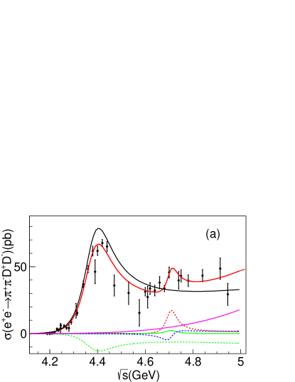
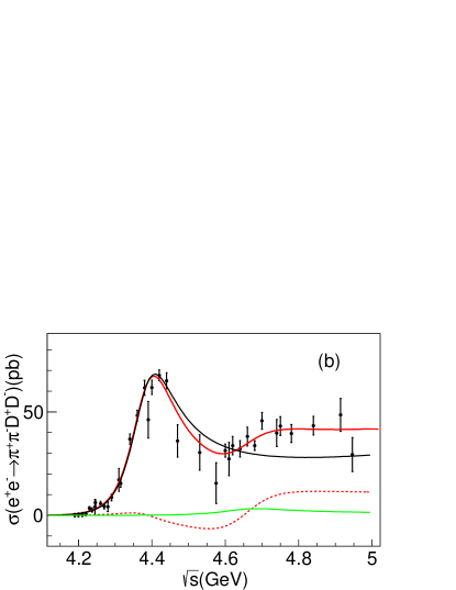
Figure 8: Cross section of the process $e^{+}e^{-}\to\pi^{+}\pi^{-}D^{+}D^{-}$ and fit with the coherent sum of two BW functions and a phase space term (Solution IV) (a), and with the coherent sum of two BW functions only (Solution II) (b). Other solutions of (a) and (b) could be found in Table 2 and 3, respectively. Dots with error bars are data with the statistical uncertainties and the red lines show the best fit results. For (a), the black, green, and pink solid lines describe $BW_{0}$, $BW_{1}$, and $\Phi_{4}$ components, respectively, and the red, green, and blue dashed lines describe interferences between $BW_{0}$ and $BW_{1}$, $BW_{0}$ and $\Phi_{4}$, and $BW_{1}$ and $\Phi_{4}$, respectively. For (b), the black and green solid lines describe $BW_{0}$ and $BW_{1}$ components, respectively, and the red dashed line describes the inteference between $BW_{0}$ and $BW_{1}$. (color version online). The fit qualities are tested using a $\chi^{2}$-test method, with $\chi^{2}/\rm{n.\ d.\ f.}=$47.1/28 and 46.1/30 for (a) and (b), respectively. The $\rm{n.\ d.\ f.}$ denotes the number of degrees of freedom. The $\chi^{2}$ function is constructed as $\chi^{2}=\Sigma\frac{(\sigma_{i}-\sigma^{fit}_{i})^{2}}{\delta_{i}^{2}}$, here, $\sigma_{i}$ and $\sigma^{fit}_{i}$ are the measured and fitted cross section of the $i^{th}$ data sample, respectively, and $\delta_{i}$ is the standard deviation of the measured cross section, which includes the statistical uncertainties only.

For data samples where no significant $e^{+}e^{-}\rightarrow\pi^{+}\pi^{-}D^{+}D^{-}$ signal peaks are observed (statistical significance smaller than $5\sigma$), the upper limits on the cross section are calculated using a Bayesian method 2003UPL . By fitting the $RM(D^{+}\pi_{d}^{+}\pi_{d}^{-})$ distribution for the events in the $D^{+}$ signal region with fixed values for the signal yield, a scan of the likelihood distribution as a function of the cross section is obtained. To take the total systematic uncertainty (listed in Table 5) into consideration, the likelihood distribution is convolved with a Gaussian function with a width corresponding to the overall systematic uncertainty. The upper limit on the cross section at 90% C.L. is obtained from $\int_{0}^{\sigma}L(x)dx/\int_{0}^{\infty}L(x)dx=0.9.$ The upper limits on the cross sections are listed in Table 1.

V Resonances in the $e^{+}e^{-}\rightarrow\pi^{+}\pi^{-}D^{+}D^{-}$ Cross Section line shape

Clear resonant structures around $\sqrt{s}=$ 4.390 and 4.700 GeV can be seen in Fig. 8, and there is no significant signal at other energies, including at the expected masses of the $Y(4230)$, $Y(4360)$, and $Y(4660)$ states.

A fit to the measured $e^{+}e^{-}\rightarrow\pi^{+}\pi^{-}D^{+}D^{-}$ cross section line shape is performed with a coherent sum of two Breit-Wigner (BW) functions and a phase space term

$$\begin{split}\sigma(\sqrt{s})=|BW_{0}(\sqrt{s})+BW_{1}(\sqrt{s})e^{i\phi_{1}}\\ +ce^{i\phi_{2}}\Phi_{4}(\sqrt{s})|^{2},\end{split}$$ (4)

with the BW function defined as

$$BW_{j}(\sqrt{s})=\frac{\sqrt{12\pi{\Gamma^{e^{+}e^{-}}_{j}}\Gamma^{\rm tot}_{j}\mathscr{B}_{j}}}{s-m_{j}^{2}+im_{j}\Gamma^{\rm tot}_{j}}\sqrt{\frac{\Phi_{4}(\sqrt{s})}{\Phi_{4}(m_{j})}},$$ (5)

where $m_{j}$, $\Gamma^{\rm tot}_{j}$, and ${\Gamma^{e^{+}e^{-}}_{j}}$ are the mass, width, and electronic partial width of the $j^{th}$ resonance ($R_{j}$), respectively; $\mathscr{B}_{j}$ is the branching fraction of the decay $R_{j}\rightarrow\pi^{+}\pi^{-}D^{+}D^{-}$, $\phi_{j}$ is the relative phase between the $j^{th}$ resonance, as well as the phase space term, $\Phi_{4}(\sqrt{s})$ is the phase space factor of the four-body decay $R\rightarrow\pi^{+}\pi^{-}D^{+}D^{-}$, and $c$ is a constant describing the magnitude of $\Phi_{4}(\sqrt{s})$.

There are four solutions with the same fit quality and identical resonance parameters for $R_{0}$ and $R_{1}$ as well as $c$, but different $\Gamma^{e^{+}e^{-}}_{j}\mathscr{B}_{j}$ and $\phi_{j}$, as listed in Table 2. The fitted parameters for $R_{0}$ are in agreement with those of the $Y(4390)$ resonance observed by the BESIII Collaboration in the $e^{+}e^{-}\rightarrow\pi^{+}\pi^{-}h_{c}$ process BESIII:2016adj . The statistical significance of $R_{1}$ is determined to be $4.1\sigma$ by comparing the likelihood of the baseline fit and that of the fit without $R_{1}$.

Table 2: The fitted parameters of the cross sections of $e^{+}e^{-}\rightarrow\pi^{+}\pi^{-}D^{+}D^{-}$ with the coherent sum of two Breit-Wigner functions and a phase space term. The first uncertainties are statistical and the second systematic.

Parameters	Solution I	Solution II	Solution III	Solution IV
$c\ (\rm{MeV}^{-3/2})$	$\ \ \ \ \ \ \ \ \ \ \ \ \ \ \ \ \ (1.6\pm 0.9\pm 0.1)\times 10^{3}$
$m_{0}\ (\rm{MeV}/c^{2})$	$4373.1\pm 4.0\pm 1.0$
$\Gamma_{0}\ (\rm{MeV})$	$\ \ 146.5\pm 7.4\pm 1.1$
$m_{1}\ (\rm{MeV}/c^{2})$	$\ \ 4706\ \pm 11\ \pm 4\ \$
$\Gamma_{1}\ (\rm{MeV})$	$\ \ \ \ \ \ 45\ \pm 28\ \pm 9\ \$
$\Gamma^{e^{+}e^{-}}_{0}\mathscr{B}_{0}\ (\rm eV)$	9.3$\ \pm\$0.8$\ \pm\$1.8	9.3$\ \pm\$0.8$\ \pm\$1.3	13.0$\ \pm\$1.5$\ \pm\$1.7	9.9$\ \pm\$1.1$\ \pm\$1.4
$\Gamma^{e^{+}e^{-}}_{1}\mathscr{B}_{1}\ (\rm eV)$	11.9$\ \pm\$6.5$\ \pm\$3.2	0.2$\ \pm\$0.1$\ \pm\$0.1	0.2$\ \pm\$0.1$\ \pm\$0.1	10.8$\ \pm\$5.3$\ \pm\$2.8
$\phi_{1}\ (\rm{rad})$	4.9$\ \pm\$0.2$\ \pm\$0.0	0.3$\ \pm\$0.4$\ \pm\$0.0	1.1$\ \pm\$0.7$\ \pm\$0.0	4.1$\ \pm\$0.3$\ \pm\$0.0
$\phi_{2}\ (\rm{rad})$	4.6$\ \pm\$0.3$\ \pm\$1.0	1.6$\ \pm\$0.3$\ \pm\$1.0	1.6$\ \pm\$0.3$\ \pm\$1.0	4.5$\ \pm\$0.3$\ \pm\$1.0

If we omit the phase space term from the baseline fit, the fit quality becomes slightly worse, indicating the statistical significance of this amplitude is only $1.4\sigma$ and the solutions of this amplitude could be found in Table 3. However, the fit in the high energy region becomes very different, as shown in Fig. 8(b). For the fit with the coherent sum of two BW functions only, there are two solutions with the same fit quality and identical resonance parameters for $R_{0}$ and $R_{1}$, but different $\Gamma^{e^{+}e^{-}}_{j}$ and $\phi_{j}$, as listed in Table 3. The statistical significance of $R_{1}$ is $7.0\sigma$.

Table 3: The fitted parameters of the cross sections of $e^{+}e^{-}\rightarrow\pi^{+}\pi^{-}D^{+}D^{-}$ with the coherent sum of two Breit-Wigner functions. The uncertainties are statistical.

Parameters	Solution I	Solution II
$m_{0}\ (\rm{MeV}/c^{2})$	$4378.0\pm 8.5$
$\Gamma_{0}\ (\rm{MeV})$	$\ \ \ \ 152\pm 14$
$m_{1}\ (\rm{MeV}/c^{2})$	$\ \ 4605\pm 90$
$\Gamma_{1}\ (\rm{MeV})$	$\ \ \ \ 245\pm 67$
$\Gamma^{e^{+}e^{-}}_{0}\mathscr{B}_{0}\ (\rm{eV})$	21$\ \pm\$12	12.2$\ \pm\$5.8
$\Gamma^{e^{+}e^{-}}_{1}\mathscr{B}_{1}\ (\rm{eV})$	54$\ \pm\$15	1.3$\ \pm\$2.7
$\phi_{1}\ (\rm{rad})$	4.1$\ \pm\$0.3	5.6$\ \pm\$2.6

Other than the $R_{0}$ and $R_{1}$ contributions, we also tested the statistical significances of the possible structures around $\sqrt{s}=$ 4.245 and 4.914 GeV. By adding the $Y(4230)$ amplitude to the fit, with the mass and width fixed according to the world averaged values pdg , its significance is found to be only $0.3\sigma$. By adding a new resonance at high energy with free mass and width, the statistical significance is found to be $1.3\sigma$. Therefore, such additional structures are not considered at the upper and lower mass regions.

Note that there are four points ($\sqrt{s}$ from 4.400 to 4.600 GeV) systematically below the fitted line. Since the integrated luminosities of these data samples are very low, larger data samples are needed to draw a conclusion.

VI Evidence for $e^{+}e^{-}\rightarrow\pi^{+}\pi^{-}X(3842)$

To search for the $X(3842)$ state, the $S$ sample defined in Sec. III with the additional $K^{0}_{S}$ veto and stringent $|V_{xy}|$ and $|V_{z}|$ requirements ($|V_{xy}|<0.55$ cm and $|V_{z}|<3$ cm) is used. In order to suppress the $e^{+}e^{-}\rightarrow D_{1}(2420)^{+}D^{-}$ background, the $D_{1}(2420)$ signal is suppressed by requiring $|RM(D^{+})-m_{D_{1}(2420)^{-}}|>0.01$ GeV/$c^{2}$ and $|RM(D_{\rm{miss}}^{-})-m_{D_{1}(2420)^{+}}|>0.01$ GeV/$c^{2}$, where $m_{D_{1}(2420)^{\pm}}=2.4221$ GeV/$c^{2}$ is the known $D_{1}(2420)^{\pm}$ mass pdg .

The $RM(\pi_{d}^{+}\pi_{d}^{-})$ (equivalent to the invariant mass of $D^{+}D_{\rm miss}^{-}$) distributions in all data samples are examined. While no significant signal is observed at any single $\sqrt{s}$, there is evidence for an $X(3842)$ resonance for $\sqrt{s}$ from 4.600 to 4.700 GeV. Figure 9 shows the $RM(\pi_{d}^{+}\pi_{d}^{-})$ distributions at $\sqrt{s}=$ 4.420, 4.680 GeV, and data samples with $\sqrt{s}$ from 4.600 to 4.700 GeV.

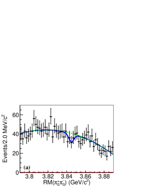
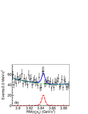
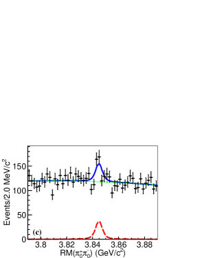
Figure 9: The $RM(\pi_{d}^{+}\pi_{d}^{-})$ distributions and the fits at $\sqrt{s}=$ 4.420 (a), 4.680 (b) GeV, and data samples with $\sqrt{s}$ from 4.600 to 4.700 GeV (c). The black dots with error bars are the $S$ sample, and the red dashed, green dash-dotted, and blue solid curves are the signal shape, background shape, and total fit, respectively (color version online). The fit qualities are tested using a $\chi^{2}$-test method, with $\chi^{2}/\rm{n.\ d.\ f.}=$26.3/45, 41.4/43, and 57.07/45 for (a), (b), and (c), respectively.

To fit the $RM(\pi_{d}^{+}\pi_{d}^{-})$ distributions, the $X(3842)$ signal shape is obtained from MC simulation of the $e^{+}e^{-}\rightarrow f_{0}(500)X(3842)\rightarrow\pi^{+}\pi^{-}D^{+}D^{-}$ process, and convolved with a Gaussian function to take the resolution difference between data and MC simulation into account. The mean and sigma values of the Gaussian function for other fits are fixed to the fit values obtained at $\sqrt{s}=$ 4.680 GeV as this sample contains the largest number of signal events. The mass and width of the $f_{0}(500)$ are taken from Ref. 2001sigma when generating MC events. The background is described with a second-order Chebychev polynomial function.

Fit results of the $RM(\pi_{d}^{+}\pi_{d}^{-})$ distributions are shown in Figs. 9(a, b, c). The signal yields (statistical significances) are $-$39 $\pm$ 18 ($-2.0\sigma$), 58 $\pm$ 24 ($1.8\sigma$), and 155 $\pm$ 38 ($4.2\sigma$) at $\sqrt{s}=$ 4.420, 4.680 GeV and data samples with $\sqrt{s}$ from 4.600 to 4.700 GeV, respectively. Furthermore, for data samples with $\sqrt{s}$ from 4.600 to 4.700 GeV, the fits are also performed by changing the fit range, the signal shape, or the background shape. In all cases, the minimum value of the $X(3842)$ resonance significance is $4.2\sigma$. The fit results at other energies are listed in Table 4. The cross sections of the $e^{+}e^{-}\rightarrow\pi^{+}\pi^{-}X(3842)\rightarrow\pi^{+}\pi^{-}D^{+}D^{-}$ process are calculated in a similar way as for other processes, and the upper limits of the cross sections are determined using a similar strategy to that described in Sec. IV. The results are also listed in Table 4.

Table 4: Results for the $e^{+}e^{-}\rightarrow\pi^{+}\pi^{-}X(3842)\rightarrow\pi^{+}\pi^{-}D^{+}D^{-}$ process. Here, $\sigma$ is the cross section of the $e^{+}e^{-}\rightarrow\pi^{+}\pi^{-}X(3842)\rightarrow\pi^{+}\pi^{-}D^{+}D^{-}$ process, where the first uncertainty is statistical and the second systematic; $S$ is the statistical significance; $\epsilon$, $(1+\delta)$, $N$, and $\sigma_{\rm ul}$ are the detection efficieny, ISR correction factor, signal yields, and the upper limit of cross section at 90% confidence level.

$\sqrt{s}^{\rm nominal}$	$\epsilon(\%)$	$(1+\delta)$	$\mathscr{L}$ ($\rm{pb}^{-1}$)	$N$		$\sigma\ (\rm{pb})$			$S$	$\sigma_{\rm{ul}}$ (pb)
4.190	3.3	0.80	570.0	1$\pm$	2	0.5$\pm$	0.8 $\pm$	0.1	$\ \ \ \ 0.6\sigma$	2.5
4.200	4.8	0.81	526.0	3$\pm$	3	0.8$\pm$	0.8 $\pm$	0.1	$\ \ \ \ 1.1\sigma$	2.6
4.210	5.8	0.82	572.1	$-$1$\pm$	1	$-$0.2$\pm$	0.4 $\pm$	0.0	-	0.9
4.220	7.0	0.83	569.1	$-$2$\pm$	2	$-$0.4$\pm$	0.4 $\pm$	0.1	-	0.7
4.230	9.1	0.83	1100.9	0$\pm$	4	0.0$\pm$	0.3 $\pm$	0.0	$\ \ \ \ 0.1\sigma$	0.6
4.237	9.7	0.84	530.0	0$\pm$	3	0.1$\pm$	0.4 $\pm$	0.0	$\ \ \ \ 0.3\sigma$	1.0
4.246	10.4	0.84	538.1	$-$3$\pm$	2	$-$0.4$\pm$	0.3 $\pm$	0.1	-	0.5
4.269	11.8	0.85	825.7	$-$8$\pm$	4	$-$0.6$\pm$	0.3 $\pm$	0.1	-	0.3
4.270	12.2	0.85	531.1	6$\pm$	4	0.6$\pm$	0.4 $\pm$	0.1	$\ \ \ \ 1.5\sigma$	1.5
4.290	12.2	0.86	502.4	0$\pm$	4	$-$0.0$\pm$	0.4 $\pm$	0.0	$\ \ \ \ 0.1\sigma$	0.9
4.315	14.8	0.87	501.2	2$\pm$	6	0.2$\pm$	0.5 $\pm$	0.0	$\ \ \ \ 0.4\sigma$	0.9
4.340	15.6	0.88	505.0	$-$8$\pm$	7	$-$0.7$\pm$	0.6 $\pm$	0.1	-	0.6
4.360	17.1	0.88	544.0	$-$7$\pm$	9	$-$0.5$\pm$	0.6 $\pm$	0.1	-	1.0
4.380	16.2	0.89	522.7	$-$19$\pm$	8	$-$1.3$\pm$	0.6 $\pm$	0.2	-	1.1
4.400	16.4	0.89	507.8	11$\pm$	12	0.8$\pm$	0.9 $\pm$	0.1	$\ \ \ \ 1.0\sigma$	4.6
4.420	18.3	0.90	1090.7	$-$39$\pm$	18	$-$1.2$\pm$	0.6 $\pm$	0.2	-	0.6
4.440	16.7	0.90	569.9	7$\pm$	15	0.5$\pm$	0.9 $\pm$	0.1	$\ \ \ \ 0.5\sigma$	3.1
4.600	19.6	0.92	586.9	31$\pm$	13	1.6$\pm$	0.7 $\pm$	0.2	$\ \ \ \ 2.5\sigma$	3.3
4.620	18.5	0.93	521.5	27$\pm$	13	1.6$\pm$	0.8 $\pm$	0.2	$\ \ \ \ 2.2\sigma$	3.4
4.640	18.8	0.93	552.4	17$\pm$	13	1.0$\pm$	0.7 $\pm$	0.1	$\ \ \ \ 1.4\sigma$	2.3
4.660	19.1	0.93	529.6	13$\pm$	13	0.8$\pm$	0.7 $\pm$	0.1	$\ \ \ \ 1.1\sigma$	2.0
4.680	19.1	0.93	1669.3	58$\pm$	24	1.0$\pm$	0.4 $\pm$	0.1	$\ \ \ \ 1.8\sigma$	1.5
4.700	19.1	0.93	536.5	1$\pm$	13	0.1$\pm$	0.7 $\pm$	0.0	$\ \ \ \ 0.1\sigma$	1.4
4.750	20.1	0.93	367.2	0$\pm$	10	$-$0.1$\pm$	0.8 $\pm$	0.0	$\ \ \ \ 0.1\sigma$	1.4
4.780	20.0	0.94	512.8	15$\pm$	12	0.9$\pm$	0.7 $\pm$	0.1	$\ \ \ \ 1.4\sigma$	2.0
4.840	20.5	0.94	527.3	$-$11$\pm$	10	$-$0.6$\pm$	0.5 $\pm$	0.1	-	0.7
4.916	20.4	0.95	208.1	$-$6$\pm$	5	$-$0.9$\pm$	0.8 $\pm$	0.1	-	1.1
4.946	20.0	0.95	160.4	$-$10$\pm$	3	$-$1.7$\pm$	0.6 $\pm$	0.2	-	0.8

VII Systematic Uncertainties

VII.1 Systematic uncertainties for the $e^{+}e^{-}\rightarrow\pi^{+}\pi^{-}D^{+}D^{-}$ cross sections

The systematic uncertainties in the cross section measurement of the $e^{+}e^{-}\rightarrow\pi^{+}\pi^{-}D^{+}D^{-}$ process stem from many sources. The systematic uncertainties associated with the detection efficiencies, including tracking TRACKPID and PID TRACKPID , are estimated as 1% for each. The systematic uncertainty associated with the integrated luminosity measurement using Bhabha ($e^{+}e^{-}\rightarrow e^{+}e^{-}$) events is estimated as 1% Lum . For the vacuum polarization factor calculation, the systematic uncertainty originates mainly from hadronic contributions, and is estimated as 0.1% according to VP . The systematic uncertainty coming from the input branching fraction of $D^{+}\rightarrow K^{-}\pi^{+}\pi^{+}$ is estimated as 1.7% pdg . Details of further systematic uncertainties are given below.

The selection efficiency is obtained from MC simulation and corrected according to the measurements with control samples selected from data directly. The efficiency correction factor $f^{v}$ is defined as

$$f^{v}=\epsilon^{v}_{\rm{data}}/\epsilon^{v}_{\rm{MC}},$$ (6)

with

$$\epsilon^{v}_{\rm{data}(\rm{MC})}=N^{v}_{\rm{signal}_{\rm{data}(\rm{MC})}}/N^{v}_{\rm{all}_{\rm{data}(\rm{MC})}},$$ (7)

where the subscript “MC” represents MC simulation and the subscript “data” represents the data sample, $N^{v}_{\rm{signal}_{\rm{data}(\rm{MC})}}$ is the number of events in the signal region of a selection criterion $v$, and $N^{v}_{\rm{all}_{\rm{data}(\rm{MC})}}$ is the number of events in the full range of $v$.

The uncertainty of $\epsilon^{v}_{\rm{data}(\rm{MC})}$

$$\sigma_{\epsilon^{v}_{\rm{data}(\rm{MC})}}=\sqrt{\frac{\epsilon^{v}_{\rm{data}(\rm{MC})}(1-\epsilon^{v}_{\rm{data}(\rm{MC})})}{N^{v}_{\rm{all}_{\rm{data}(\rm{MC})}}}},$$ (8)

and the uncertainty of $f^{v}$ is

$$\frac{\sigma^{2}_{f^{v}}}{{f^{v}}^{2}}=\frac{\sigma_{\epsilon^{v}_{\rm{data}}}^{2}}{{\epsilon_{\rm{data}}^{v}}^{2}}+\frac{\sigma_{\epsilon^{v}_{\rm{MC}}}^{2}}{{\epsilon^{v}_{\rm{MC}}}^{2}},$$ (9)

since data and MC simulation are independent. For $f^{v}=(1\pm\Delta f^{v})\pm\sigma_{f^{v}}$, if $|\frac{\Delta f^{v}}{\sigma_{f^{v}}}|<1.00$, no correction will be applied and $|\Delta f^{v}|+\sigma_{f^{v}}$ will be taken as the systematic uncertainty, where $\Delta f^{v}$ is the deviation of $f^{v}$ from 1; while if $|\frac{\Delta f^{v}}{\sigma_{f^{v}}}|>1.00$, the MC efficiency will be corrected as $\epsilon=\epsilon_{MC}\times f^{v}$, and $\sigma_{f^{v}}$ will be taken as the systematic uncertainty.

In order to avoid effects from statistical uncertainty, only data samples at $\sqrt{s}=$ 4.340, 4.360, 4.400, 4.420, 4.440, 4.600, and 4.680 GeV are used to estimate the systematic uncertainty originating from the $M(K^{-}\pi^{+}\pi^{+})$ ($RM(D^{+}\pi_{d}^{+}\pi_{d}^{-})$) mass window requirement. A constant parameter is used to fit the distributions of $f^{M(K^{-}\pi^{+}\pi^{+})}$ ($f^{RM(D^{+}\pi_{d}^{+}\pi_{d}^{-})}$) among the data samples mentioned above, and the fitted $f^{M(K^{-}\pi^{+}\pi^{+})}$ ($f^{RM(D^{+}\pi_{d}^{+}\pi_{d}^{-})}$) and $\sigma_{f^{M(K^{-}\pi^{+}\pi^{+})}}$ ($\sigma_{f^{RM(D^{+}\pi_{d}^{+}\pi_{d}^{-})}}$) values are 0.986 $\pm$ 0.003 (0.984 $\pm$ 0.005), the value of $\Big{|}\frac{\Delta f^{M(K^{-}\pi^{+}\pi^{+})}}{\sigma_{f^{M(K^{-}\pi^{+}\pi^{+})}}}\Big{|}$ ($\Big{|}\frac{\Delta f^{RM(D^{+}\pi_{d}^{+}\pi_{d}^{-})}}{\sigma_{f^{RM(D^{+}\pi_{d}^{+}\pi_{d}^{-})}}}\Big{|}$) is 5.6 (2.8), therefore, the systematic uncertainty is taken as 0.3% (0.5%) and $f^{M(K^{-}\pi^{+}\pi^{+})}$ ($f^{RM(D^{+}\pi_{d}^{+}\pi_{d}^{-})}$) is set to be 0.986 (0.984).

In order to avoid effects from the statistical uncertainty, the same set of data samples as mentioned in the previous paragraph is used to estimate the systematic uncertainties originating from the fit range and background shape of $RM(D^{+}\pi_{d}^{+}\pi_{d}^{-})$. The systematic uncertainty coming from the choice of the fit range is estimated by varying the limits of the fit range from (1.75, 1.96) GeV/$c^{2}$ to (1.77, 1.97) GeV/$c^{2}$. The background shape is varied from the first-order Chebychev polynomial function to a second-order one at $\sqrt{s}=$ 4.340 and 4.360 GeV, and the second-order Chebychev polynomial function to the first-order one at $\sqrt{s}=$ 4.400, 4.420, 4.440, 4.600, and 4.680 GeV. The largest difference of the cross section compared with the baseline value among the data samples mentioned above is taken as a systematic uncertainty of 1.6% (1.7%) for the fit range (background shape).

The systematic uncertainty stemming from the $p/\bar{p}$ veto, which is caused by the difference in mis-identification probability of $K$ to $p/\bar{p}$ between data and MC simulation, is estimated by the control sample of $J/\psi\rightarrow K_{S}^{0}K^{-}\pi^{+}+c.c.$ with the BESIII $J/\psi$ sample KsKpi . The values of $f^{K\nrightarrow p}$ and $\sigma_{f^{K\nrightarrow p}}$ are 0.996 $\pm$ 0.003, and the value of $|\frac{\Delta f^{K\nrightarrow p}}{\sigma_{f^{K\nrightarrow p}}}|$ is 1.4, therefore, the systematic uncertainty is taken as 0.3% and $f^{K\nrightarrow p}$ is set to 0.996. Similarly, using the control sample of $e^{+}e^{-}\rightarrow\pi^{+}\pi^{-}J/\psi$ at $\sqrt{s}=4.260$ GeV 2013Zc_3900 , $f^{L/\Delta_{L}}$ and $f^{V_{xy,\ z}}$ are estimated by performing a secondary vertex fit on $\pi^{+}$ and $\pi^{-}$ pair and comparing $V_{xy,\ z}$ of $\pi^{+}$, $\pi^{-}$, and lepton pair from $J/\psi$ in data and MC simulation, respectively. The values of $f^{L/\Delta_{L}}$ ($f^{V_{xy,\ z}}$) and $\sigma_{f^{L/\Delta_{L}}}$ ($\sigma_{f^{V_{xy,\ z}}}$) are 0.992 $\pm$ 0.010 (0.997 $\pm$ 0.001), $f^{L/\Delta_{L}}$ ($f^{V_{xy,\ z}}$) is set as 0.992 (0.997), and the systematic uncertainty associated with the $L_{\pi_{d}^{+}\pi_{d}^{-}}/\Delta_{L_{\pi_{d}^{+}\pi_{d}^{-}}}$ requirement for the $K_{S}^{0}$ veto ($V_{xy,\ z}$ requirements) is 1.0% (0.1%).

Table 5: Systematic uncertainties (%) from the scale factors $f_{1}$ and $f_{2}$ ($f_{1}$ and $f_{2}$), $\psi(3770)$ and $D_{1}(2420)^{+}$ shapes, including a new Breit-Wigner shape in the high energy region when parameterizing each subprocess cross section line shape, uncertainty of $\omega_{i}$ ($\omega_{i}$), and angular distribution modeling of $e^{+}e^{-}\rightarrow D_{1}(2420)^{+}D^{-}$ decay (helamp). The last column shows the total systematic uncertainty obtained by summing up all sources of systematic uncertainties in quadrature assuming they are uncorrelated.

$\sqrt{s}^{\rm nominal}$	$f_{1}$ and $f_{2}$	$\psi(3770)$ shape	$D_{1}(2420)^{+}$ shape	New Breit-Wigner	$\omega_{i}$	helamp	Total
4.190	0.0	0.0	-	0.0	14.4	-	16.6
4.200	0.0	0.0	-	0.0	19.3	-	21.0
4.210	0.0	0.0	-	0.0	16.8	-	18.7
4.220	0.0	0.0	-	0.0	0.8	-	8.3
4.230	0.6	1.7	-	0.9	0.8	-	8.6
4.237	0.0	1.6	-	2.3	0.6	-	8.8
4.245	0.5	0.3	-	0.3	1.8	-	8.5
4.246	0.5	0.7	-	3.0	7.8	-	11.8
4.260	0.2	0.9	-	0.7	0.4	-	8.4
4.270	0.0	0.5	-	1.2	0.7	-	8.4
4.280	0.2	1.4	-	1.4	0.5	-	8.5
4.290	0.1	0.1	-	1.8	0.5	-	8.5
4.310	1.5	0.3	-	1.4	0.4	-	8.5
4.315	0.1	0.4	-	0.3	0.2	-	8.3
4.340	0.1	0.4	0.7	1.2	0.3	0.5	8.4
4.360	0.2	0.0	0.2	2.0	0.1	0.2	8.5
4.380	0.2	0.6	0.1	0.4	0.3	0.8	8.4
4.390	0.1	0.3	1.2	1.0	0.8	0.3	8.5
4.400	0.1	0.5	1.0	0.1	0.7	0.6	8.4
4.420	0.0	0.1	0.6	0.1	1.8	0.8	8.5
4.440	0.2	0.9	3.3	0.2	1.5	0.4	9.1
4.470	0.2	1.4	0.9	0.5	6.6	0.2	10.7
4.530	0.2	0.2	0.4	0.3	6.0	0.7	10.3
4.575	0.5	0.3	1.8	0.0	2.1	1.3	8.8
4.600	0.5	0.4	1.7	2.8	0.8	0.8	9.0
4.612	0.1	0.2	0.0	0.3	1.2	0.5	8.4
4.620	0.1	1.5	0.9	0.3	1.1	0.4	8.5
4.640	0.5	0.2	0.8	1.6	1.4	0.2	8.6
4.660	0.2	0.9	0.3	2.6	1.0	0.2	8.8
4.680	0.2	0.4	0.9	0.0	0.4	0.1	8.3
4.700	0.0	0.8	0.7	2.3	0.5	0.0	8.7
4.740	0.1	0.1	2.1	0.5	0.8	0.3	8.6
4.750	0.5	0.8	0.6	1.9	1.2	0.2	8.7
4.780	0.1	0.3	0.2	0.4	0.8	0.3	8.3
4.840	0.3	0.9	0.7	0.5	0.6	1.9	8.6
4.914	0.0	0.6	1.1	1.1	1.4	1.7	8.7
4.946	0.8	0.6	0.4	0.6	1.6	0.9	8.6

$e^{+}e^{-}\rightarrow\pi^{+}\pi^{-}\psi(3770)\rightarrow\pi^{+}\pi^{-}D^{+}D^{-}$ and $e^{+}e^{-}\rightarrow D_{1}(2420)^{+}D^{-}\rightarrow\pi^{+}\pi^{-}D^{+}D^{-}$ processes are simulated when estimating $\omega_{i}$, for the estimation of the systematic uncertainty stemming from the $\psi(3770)$ ($D_{1}(2420)^{+}$) shape, alternative MC samples are produced by varying the width of $\psi(3770)$ ($D_{1}(2420)^{+}$) by one standard deviation of its world average value pdg . The difference of the cross section of $e^{+}e^{-}\rightarrow\pi^{+}\pi^{-}D^{+}D^{-}$ process compared with the baseline value is taken as the systematic uncertainty as listed in Table 5.

In Sec. II, $e^{+}e^{-}$ is assumed to annihilate into $D_{1}(2420)^{+}D^{-}$ directly, and the systematic uncertainty stemming from modeling the angular distribution of the $e^{+}e^{-}\rightarrow D_{1}(2420)^{+}D^{-}$ process is estimated by repeating the analysis procedure with the new model. For the $e^{+}e^{-}\rightarrow D_{1}(2420)^{+}D^{-}$ process, two extreme cases of the angular distribution following $1+\cos^{2}\theta_{D_{1}}$ and $1-\cos^{2}\theta_{D_{1}}$ are assumed, where $\theta_{D_{1}}$ is the helicity angle of the $D_{1}(2420)^{+}$ in the rest frame of the initial $e^{+}e^{-}$ system. The fractions of these two cases are estimated by fitting to the $\rm{cos}\ \theta_{D^{+}}$ distribution, where $\theta_{D^{+}}$ is the polar angle of $D^{+}$ in the rest frame of the initial $e^{+}e^{-}$ system, the detection efficiency of $e^{+}e^{-}\rightarrow D_{1}(2420)^{+}D^{-}\rightarrow\pi^{+}\pi^{-}D^{+}D^{-}$ process is recalculated according to the detection efficiencies and fractions of these two cases, and the cross section of $e^{+}e^{-}\rightarrow\pi^{+}\pi^{-}D^{+}D^{-}$ process is recalculated as well. The difference of the cross section of the $e^{+}e^{-}\rightarrow\pi^{+}\pi^{-}D^{+}D^{-}$ process compared with the baseline value is taken as the systematic uncertainty as listed in Table 5.

In Sec. III, the normalization factor $f_{1}$ ($f_{2}$) in the $B$ sample is estimated by assuming a linear background distribution in $M(K^{-}\pi^{+}\pi^{+})$ ($RM(D^{+}\pi_{d}^{+}\pi_{d}^{-})$). A second-order Chebychev polynomial function is used as the background shape to fit the $M(K^{-}\pi^{+}\pi^{+})$ ($RM(D^{+}\pi_{d}^{+}\pi_{d}^{-})$) distribution to estimate $f_{1}$ ($f_{2}$). The signal shape is modelled by the $M(K^{-}\pi^{+}\pi^{+})$ ($RM(D^{+}\pi_{d}^{+}\pi_{d}^{-})$) distributions in MC simulation of each subprocess weighted according to fractions of each subprocess, $\omega_{i}$, and convolved with a Gaussian function to take the resolution difference between data and MC simulation into consideration. $\omega_{i}$ is re-estimated according to the new $f_{1}$ and $f_{2}$, and the cross section of the $e^{+}e^{-}\rightarrow\pi^{+}\pi^{-}D^{+}D^{-}$ process is recalculated. The difference from the baseline value is taken as the systematic uncertainty originating from this source as listed in Table 5.

The systematic uncertainty due to the uncertainty of the fraction of each subprocess, $\omega_{i}$, is estimated by varying $\omega_{i}$ 500 times according to the convariant matrix in the simultaneous fit of $RM(D^{+})$, $RM(D_{\rm{miss}}^{-})$, and $RM(\pi_{d}^{+}\pi_{d}^{-})$ distributions for each $\sqrt{s}$. In each iteration, the difference between the cross section of the $e^{+}e^{-}\rightarrow\pi^{+}\pi^{-}D^{+}D^{-}$ process and the baseline value is calculated, and the distribution of the differences is sampled at each $\sqrt{s}$, the width of the distribution is taken as the systematic uncertainty as listed in Table 5.

The systematic uncertainty of the radiative correction is calculated by using the kkmc package. Initially, the observed signal events are assumed to originate from the $Y(4260)$ resonance to obtain the efficiency and ISR correction factor. Then, the measured line shape is used as input to calculate the efficiency and ISR correction again. This procedure is repeated until the difference between the subsequent iteration is comparable with the statistical uncertainty. The systematic uncertainty due to the input line shapes of subprocesses is estimated as described below.

The input line shape of each subprocess is varied 500 times according to the convariant matrix when parametrizing, and the $\sum\omega_{i}\epsilon_{i}(1+\delta)_{i}$ distribution is sampled at $\sqrt{s}=$ 4.380, 4.390, 4.400, 4.420, and 4.440 GeV. The maximum fraction of width and mean values of the distributions, 2.8%, is taken as the systematic uncertainty due to the input line shapes in the ISR correction. Moreover, new resonances around $\sqrt{s}=$ 4.700 GeV are added when parameterizing the line shape of each subprocess since there is an evidence around $\sqrt{s}=4.700$ GeV in the $e^{+}e^{-}\rightarrow\pi^{+}\pi^{-}D^{+}D^{-}$ cross section line shape, and the difference is taken as the systematic uncertainty associated with the new BW resonance in the high energy regions as listed in Table 5.

Table 5 summarizes the total systematic uncertainties. The total systematic uncertainty at each $\sqrt{s}$ is obtained by summing up all sources of systematic uncertainties in quadrature, assuming that they are uncorrelated.

VII.2 Systematic uncertainties in resonance parameters

The systematic uncertainties when parameterizing the resonances in the
$e^{+}e^{-}\rightarrow\pi^{+}\pi^{-}D^{+}D^{-}$ cross section line shape mainly stem from the absolute $\sqrt{s}$ measurement, the $\sqrt{s}$ spread, global shift of the $\sqrt{s}$ for data samples taken in the same period, and the systematic uncertainty of the cross section measurement.

The absolute $\sqrt{s}$ of data samples with $\sqrt{s}$ smaller than 4.610 GeV are measured with dimuon events, with an uncertainty of
$\pm$ 0.8 MeV, while those with $\sqrt{s}$ larger than or equal to 4.610 GeV are measured with $\Lambda_{c}^{+}\bar{\Lambda}_{c}^{-}$ events with an uncertainty of $\pm$ 0.6 MeV.
Thus, 0.8 MeV is taken as the systematic uncertainty, and propagates to the masses of the resonances by the same amount.

The systematic uncertainty from the $\sqrt{s}$ spread is estimated by convolving the fit formula with a Gaussian function with a width of 1.6 MeV, which is the beam spread, determined from measurement results of the Beam Energy Measurement System 2011BEMS at other $\sqrt{s}$.

The systematic uncertainty from global shift of the $\sqrt{s}$ for data samples taken in the same period is estimated by shifting the $\sqrt{s}$ of corresponding data samples by 3 MeV and deviations of parameters is taken as the systematic uncertainties.

The systematic uncertainty from the cross section measurement is divided into two parts. The first part covers uncorrelated systematic uncertainties among the different data samples (those in Table 5). The corresponding systematic uncertainty is estimated by including the uncertainty in the fit to the cross section, and taking the differences on the parameters as the systematic uncertainties. The second part includes all the other systematic uncertainties (8.3%), which is common for all data samples, and only affects the $\Gamma^{e^{+}e^{-}}_{j}\mathscr{B}_{j}$ measurement.

Table 6 summarizes the systematic uncertainties in the parameters of resonances for the four solutions. The total systematic uncertainty is obtained by summing up all sources of systematic uncertainties in quadrature, assuming they are uncorrelated.

Table 6: Systematic uncertainties in the measurement of the resonances parameters. $\sqrt{s}$ represents the systematic uncertainty from the center-of-mass measurement. $\sqrt{s}$ shift represents the systematic uncertainty from the global shift of $\sqrt{s}$ for data samples taken in the same period. Cross $\rm{section}_{a(b)}$ represents the systematic uncertainty from the cross section measurements which are uncorrelated (common) in each data sample. The units of $m_{i}$, $\Gamma^{\rm{tot}_{i}}$, $c$, $\Gamma^{e^{+}e^{-}}_{j}\mathscr{B}_{j}$, and $\phi_{j}$ are MeV/$c^{2}$, MeV, MeV^-3/2, eV and rad, respectively.

	Sources	$m_{0}$	$\Gamma_{0}$	$m_{1}$	$\Gamma_{1}$	$c$	$\Gamma^{e^{+}e^{-}}_{0}\mathscr{B}_{0}$	$\Gamma^{e^{+}e^{-}}_{1}\mathscr{B}_{1}$	$\phi_{0}$	$\phi_{1}$
Solution I	$\sqrt{s}$	0.8	-	0.8	-	-	-	-	-	-
	$\sqrt{s}$ shift	2.0	0.7	0.6	0.0	70	0.1	0.0	0.0	1.0
	$\sqrt{s}$ spread	0.0	0.1	0.1	0.3	92	1.6	1.3	0.0	1.0
	Cross $\rm{Section}_{a}$	0.6	1.1	3.8	8.8	58	0.1	2.9	-	-
	Cross $\rm{Section}_{b}$	-	-	-	-	-	0.8	0.0	-	-
	Overall	2.2	1.3	3.9	8.8	13$\times$10	1.8	3.2	0.0	1.4
Solution II	$\sqrt{s}$	0.8	-	0.8	-	-	-	-	-	-
	$\sqrt{s}$ shift	2.0	0.7	0.6	0.0	70	0.1	0.0	0.0	3.2
	$\sqrt{s}$ spread	0.0	0.1	0.1	0.3	92	1.0	0.0	0.0	0.0
	Cross $\rm{Section}_{a}$	0.6	1.1	3.8	8.8	58	0.1	0.1	-	-
	Cross $\rm{Section}_{b}$	-	-	-	-	-	0.8	0.0	-	-
	Overall	2.2	1.3	3.9	8.8	13$\times$10	1.3	0.1	0.0	3.2
Solution III	$\sqrt{s}$	0.8	-	0.8	-	-	-	-	-	-
	$\sqrt{s}$ shift	2.0	0.7	0.6	0.0	70	0.1	0.0	0.1	3.1
	$\sqrt{s}$ spread	0.0	0.1	0.1	0.3	92	1.5	0.0	0.0	3.1
	Cross $\rm{Section}_{a}$	0.6	1.1	3.8	8.8	58	0.3	0.1	-	-
	Cross $\rm{Section}_{b}$	-	-	-	-	-	0.8	0.0	-	-
	Overall	2.2	1.3	3.9	8.8	13$\times$10	1.7	0.1	0.1	4.4
Solution IV	$\sqrt{s}$	0.8	-	0.8	-	-	-	-	-	-
	$\sqrt{s}$ shift	2.0	0.7	0.6	0.0	70	0.1	0.0	0.0	1.0
	$\sqrt{s}$ spread	0.0	0.1	0.1	0.3	92	1.1	1.2	0.0	0.0
	Cross $\rm{Section}_{a}$	0.6	1.1	3.8	8.8	58	0.0	2.5	-	-
	Cross $\rm{Section}_{b}$	-	-	-	-	-	0.8	0.0	-	-
	Overall	2.2	1.3	3.9	8.8	13$\times$10	1.4	2.8	0.0	1.0

VII.3 Systematic uncertainties in $X(3842)$ measurement

Except for the fit range and the background shape of the $RM(\pi_{d}^{+}\pi_{d}^{-})$, $RM(D^{+})$ and $RM(D_{\rm{miss}}^{-})$ mass window requirements, other sources of systematic uncertainties associated with this measurement are the same as those in Sec. VII.1, but with the fit range and background shape of $RM(D^{+}\pi_{d}^{+}\pi_{d}^{-})$ excluded.

The systematic uncertainty originating from the fit range of $RM(\pi_{d}^{+}\pi_{d}^{-})$ is estimated by varying the limits of the fit range from (3.79, 3.89) GeV/$c^{2}$ to (3.81, 3.91) GeV/$c^{2}$. The difference of the cross section from the baseline value in the data sample at $\sqrt{s}=4.680$ GeV is taken as the systematic uncertainty, and is 10.4%. The background shape is varied from a second-order Chebychev polynomial function to a first order one in the data sample taken at $\sqrt{s}=4.680$ GeV, the difference of the cross section compared with the baseline value is taken as the systematic uncertainty, and is 1.9%.

The systematic uncertainty stemming from the $RM(D^{+})$ and $RM(D_{\rm{miss}}^{-})$ mass window requirements, which is mainly caused by the difference between distributions of data and MC simulation in the corresponding selection criterion ranges, is estimated by producing alternative MC samples where the mass and width of $f_{0}(500)$ are varied by one standard deviation in the data sample at $\sqrt{s}=4.680$ GeV. The difference of the cross section compared with the baseline value is taken as the systematic uncertainty, and is 1.9%.

The total systematic uncertainty for data samples with $\sqrt{s}$ smaller than or equal to 4.315 GeV are equal to 12.9% , and for those with $\sqrt{s}$ larger than 4.315 GeV are equal to 13.1% by summing up all sources of systematic uncertainties in quadrature, assuming they are uncorrelated.

VIII Summary

Using data samples taken at $\sqrt{s}$ from 4.190 to 4.946 GeV, the cross section of the $e^{+}e^{-}\rightarrow\pi^{+}\pi^{-}D^{+}D^{-}$ process is reported for the first time by a partial reconstruction method.

In the cross section of the $e^{+}e^{-}\rightarrow\pi^{+}\pi^{-}D^{+}D^{-}$ process, a structure with 0.3$\sigma$ significance is visible around $\sqrt{s}=4.245$ GeV. This might be the $Y(4230)$ resonance, however, due to its low significance, it is not possible to assign it to the $Y(4230)$ or the $Y(4260)$ state.

By fitting the $e^{+}e^{-}\rightarrow\pi^{+}\pi^{-}D^{+}D^{-}$ cross section line shape, we observe a resonance with a mass of (4373.1 $\pm$ 4.0 $\pm$ 2.2) MeV/$c^{2}$ and a width of (146.5 $\pm$ 7.4 $\pm$ 1.3) MeV, which is in agreement with the $Y(4390)$. There is evidence with a statistical significance of 4.1$\sigma$ for a second resonance with a mass of (4706 $\pm$ 11 $\pm$ 4) MeV/$c^{2}$ and a width of (45 $\pm$ 28 $\pm$ 9) MeV. The first uncertainties are statistical and the second are systematic.

The $X(3842)$ resonance is searched for in the $RM(\pi_{d}^{+}\pi_{d}^{-})$ distribution and evidence is found in the $M(\pi_{d}^{+}\pi_{d}^{-})$ distribution in data samples with $\sqrt{s}$ from 4.600 to 4.700 GeV, and its significance is $4.2\sigma$. By comparing this study with previous studies, the cross section of the $e^{+}e^{-}\rightarrow\pi^{+}\pi^{-}\psi(3770)\rightarrow\pi^{+}\pi^{-}D^{+}D^{-}$ process peaks around 4.390 GeV which indicates this process might be produced via the $Y(4390)$ state 2019HY ; 2020ZY ; the process $e^{+}e^{-}\rightarrow\pi^{+}\pi^{-}\psi_{2}(3823)(\rightarrow\gamma\chi_{c1})$ peaks around $\sqrt{s}=4.360$ and $4.420$ GeV, which means this process might be produced via the $Y(4360)$ and the $\psi(4415)$ 2015X3823 resonances. There is evidence that the cross section of the $e^{+}e^{-}\rightarrow\pi^{+}\pi^{-}X(3842)$ process peaks at $\sqrt{s}$ from 4.600 to 4.700 GeV, but no significant signal is observed in samples collected at $\sqrt{s}$ around 4.400 GeV. This indicates that the production mechanism of the $e^{+}e^{-}\rightarrow\pi^{+}\pi^{-}\psi(1D)$ processes might be different and could proceed via different $Y$ or $\psi$ states. More data samples and more precise measurements are needed to reveal the mechanism 2020BESWP .

References

(1)
P. A. Zyla et al. (Particle Data Group), Prog. Theor. Exp. Phys. 2020, 083C01 (2020) and 2021 update.
(2)
N. Brambilla, A. Pineda, J. Soto, and A. Vairo,
Rev. Mod. Phys. 77, 1423 (2005).
(3)
N. Brambilla et al.,
Eur. Phys. J. C 71, 1534 (2011).
(4)
N. Brambilla, S. Eidelman, P. Foka, S. Gardner, A. S. Kronfeld, M. G. Alford, R. Alkofer, M. Butenschoen, T. D. Cohen, and J. Erdmenger, et al.
Eur. Phys. J. C 74, no.10, 2981 (2014).
(5) E. Eichten, K. Gottfried, T. Kinoshita, K. D. Lane, and T. M. Yan,
Phys. Rev. D 17, 3090 (1978).
(6) S. Godfrey and N. Isgur,
Phys. Rev. D 32, 189 (1985).
(7) T. Barnes, S. Godfrey, and E. S. Swanson,
Phys. Rev. D 72, 054026 (2005).
(8)
M. Ablikim et al. [BES Collaboration],
Phys. Lett. B 660, 315 (2008).
(9)
A. J. Bevan et al. [BaBar and Belle Collaborations],
Eur. Phys. J. C 74, 3026 (2014).
(10)
B. Aubert et al. [BaBar Collaboration],
Phys. Rev. Lett. 95, 142001 (2005).
(11)
B. Aubert et al. [BaBar Collaboration],
Phys. Rev. Lett. 98, 212001 (2007).
(12)
X. L. Wang et al. [Belle Collaboration],
Phys. Rev. Lett. 99, 142002 (2007).
(13)
T. V. Uglov, Y. S. Kalashnikova, A. V. Nefediev, G. V. Pakhlova,
and P. N. Pakhlov,
JETP Lett. 105, 1 (2017).
(14)
N. Brambilla, S. Eidelman, C. Hanhart, A. Nefediev, C. P. Shen, C. E. Thomas, A. Vairo, and C. Z. Yuan,
Phys. Rept. 873, 1 (2020).
(15)
F. K. Guo, C. Hanhart, U. G. Meißner, Q. Wang, Q. Zhao, and B. S. Zou,
Rev. Mod. Phys. 90, 015004 (2018).
(16)
H. X. Chen, W. Chen, X. Liu, and S. L. Zhu,
Phys. Rept. 639, 1 (2016).
(17)
A. J. Bevan et al. [BaBar and Belle Collaborations], Eur. Phys. J. C. 74, 3026 (2014)
(18)
M. Ablikim et al. [BESIII Collaboration], Chin. Phys. C 42, 083001 (2018).
(19)
M. Ablikim et al. [BESIII Collaboration], Phys. Rev. D 101, 112008 (2020).
(20)
M. Ablikim et al. [BESIII Collaboration], Phys. Rev. D 104, 032012 (2021).
(21)
M. Ablikim et al. [BESIII Collaboration],
Phys. Rev. Lett. 122, 102002 (2019).
(22)
M. Ablikim et al. [BESIII Collaboration],
Phys. Lett. B 804, 135395 (2020).
(23)
M. Ablikim et al. [BESIII Collaboration],
Phys. Rev. D 100, 032005 (2019).
(24)
M. Ablikim et al. [BESIII Collaboration],
Phys. Rev. Lett. 115, 011803 (2015).
(25)
R. Aaij et al. [LHCb Collaboration],
J. High Energ. Phys. 1907, 035 (2019).
(26)
M. Ablikim et al. [BESIII Collaboration],
Nucl. Instrum. Meth. A 614, 345 (2010).
(27)
C. H. Yu et al.,
Proceedings of IPAC2016, Busan, Korea, 2016,
doi:10.18429/JACoW-IPAC2016-TUYA01.
(28)
X. Li et al., Radiat. Detect. Technol. Methods 1, 13 (2017);
Y. X. Guo et al., Radiat. Detect. Technol. Methods 1, 15 (2017);
P. Cao et al., Nucl. Instrum. Meth. A 953, 163053 (2020).
(29)
M. Ablikim et al. [BESIII Collaboration], Chin. Phys. C 40, 063001 (2016).
(30)
M. Ablikim et al. [BESIII Collaboration], Chin. Phys. C 45, 103001 (2021).
(31)
M. Ablikim et al. [BESIII Collaboration],
[arXiv:2203.03133 [hep-ex]].
(32)
M. Ablikim et al. [BESIII Collaboration],
[arXiv:2203.04289 [hep-ex]].
(33)
M. Ablikim et al. [BESIII Collaboration],
Chinese Physics C 39 (2015): 093001.
(34) S. Agostinelli et al. [GEANT4 Collaboration],
Nucl. Instrum. Meth. A 506, 250 (2003).
(35) S. Jadach, B. F. L. Ward, and Z. Was,
Comput. Phys. Commun. 130, 260 (2000); Phys. Rev. D 63, 113009 (2001).
(36)
D. J. Lange, Nucl. Instrum. Meth. A 462, 152 (2001);
R. G. Ping, Chin. Phys. C 32, 599 (2008).
(37)
J. C. Chen, G. S. Huang, X. R. Qi, D. H. Zhang, and Y. S. Zhu,
Phys. Rev. D 62, 034003 (2000);
R. L. Yang, R. G. Ping and H. Chen,
Chin. Phys. Lett. 31, 061301 (2014).
(38) P. Golonka and Z. Was, Eur. Phys. J. C 45, 97 (2006).
(39)
J. Conrad et al., Phys. Rev. D 67, 012002 (2003).
(40)
M. Ablikim et al. [BESIII Collaboration],
Phys. Rev. Lett. 118, 092002 (2017).
(41)
E. M. Aitala et al.
[Fermilab E791 Collaboration],
Phys. Rev. Lett. 86, 770 (2001).
(42)
M. Ablikim et al. [BESIII Collaboration], Phys. Rev. D 101, 112008 (2020).
(43)
M. Ablikim et al. [BESIII Collaboration],
Phys. Rev. Lett. 110, 252001 (2013).
(44)
S. Actis et al.,
Eur. Phys. J. C 66, 585 (2010).
(45)
M. Ablikim et al. [BESIII Collaboration],
Phys. Rev. Lett. 126, 092002 (2021).
(46)
M. Ablikim et al. [BESIII Collaboration],
Phys. Rev. Lett. 118, 092001 (2017).
(47)
E. V. Abakumova et al.,
Nucl. Instrum. Meth. A 659, 21 (2011).
(48)
M. Ablikim et al. [BESIII Collaboration], Chin. Phys. C 44 040001 (2020).