Assouad-like dimensions of a class of random Moran measures II – non-homogeneous Moran sets

Abstract.

In this paper, we determine the almost sure values of the $\Phi$-dimensions of random measures $\mu$ supported on random Moran sets in ${\mathbb{R}}^{d}$ that satisfy a uniform separation condition. This paper generalizes earlier work done on random measures on homogeneous Moran sets [17] to the case of unequal scaling factors. The $\Phi$-dimensions are intermediate Assouad-like dimensions with the (quasi-)Assouad dimensions and the $\theta$-Assouad spectrum being special cases.

The almost sure value of $\dim_{\Phi}\mu$ exhibits a threshold phenomena, with one value for “large” $\Phi$ (with the quasi-Assouad dimension as an example of a “large” dimension) and another for “small” $\Phi$ (with the Assouad dimension as an example of a “small” dimension). We give many applications, including where the scaling factors are fixed and the probabilities are uniformly distributed. The almost sure $\Phi$ dimension of the underlying random set is also a consequence of our results.

1. Introduction

A dimension provides a way of quantifying the size of a set. In the context of subsets of a metric space, there are many different dimensions that have been defined and each describes slightly different geometric properties of the subset. Two well-known examples of this are the Hausdorff and box-counting dimensions, which are both global measures of the geometry of the given subset. It is also of substantial interest to understand the local variation in the geometry and for this other dimensions have been introduced including the (upper and lower) Assouad dimensions and variations. The Assouad dimensions [1, 6, 20, 21], the less extreme quasi-Assouad dimensions [4, 11, 22], the $\theta$-spectrum [10], and (the most general of these) the intermediate $\Phi$-dimensions [10, 12] all quantify various aspects of the “thickest” and “thinnest” parts of the set. These same Assouad-like dimensions are all also available to quantify Borel measures on metric spaces [7, 15, 16].

The $\Phi$-dimensions range between the box dimensions and the Assouad dimensions and are also locally defined. However, they differ in the depth of scales that they consider and thus can provide precise information about the set or measure (see Section 2 for definitions). In this paper we extend the investigation of the $\Phi$-dimensions of random $1$-variable measures on homogeneous Moran sets [17] to the case of random measures supported on random Moran sets with multiple scaling factors for the similarities.

The study of the dimensional properties of random fractal objects is well-established, with some early papers investigating the almost sure Hausdorff dimension [5, 14], while more recently the Assouad and related dimensions have also been investigated [8, 9, 13, 17, 24, 25].

By a random Moran measure we mean a random Borel probability measure supported on a random Moran construction in ${\mathbb{R}}^{D}$ (see Section 3 for the precise details of the construction); our construction can also be described as a random $1$-variable fractal measure. The support of the measure is constructed by a random iterative procedure, where at each stage we replace each component of the set with a random (but uniformly bounded) number of randomly scaled, separated, compact, and similar subsets. A random Borel probability measure is then defined on the random limiting set by a similar iterative process which subdivides the total mass by randomly choosing a set of probabilities at each step. The process produces a $1$-variable fractal measure since at each level we make one random choice and use that same choice for all subdivisions on that level. Specifically, at level $n$ we choose $K_{n}$ random geometric scaling factors for the similarities and $K_{n}$ random probabilities to use in subdividing the mass and use these $2K_{n}$ choices for every subdivision at that level. This is in contrast with the stochastically self-similar (or $\infty$-variable) construction where the choice is made independently for each subdivision. We make a blanket separation assumption which can be thought of as a uniform strong convex separation condition.

For any dimension function $\Phi$, the $\Phi$-dimension of the resulting random measure $\mu_{\omega}$ is almost surely constant and this value depends on how $\Phi$ compares to the threshold function $\Psi(t)=\log|\log t|/|\log t|$ near $0$; this behavior is similar to what was seen in [13, 17, 25]. For $\Phi\ll\Psi$ (the “small” dimension functions $\Phi$, such as the Assouad dimension), the computations of the almost sure values of the upper and lower $\Phi$-dimensions of the random measure $\mu_{\omega}$ are quite similar to the homogeneous (same scaling factor for all children) case dealt with in [17]. These computations involve the almost sure maximum and almost sure minimum of ratios of the logarithm of a probability to the logarithm of a scaling factor. Furthermore, the almost sure value of the $\Phi$-dimension is the same for all small dimension functions.

In contrast, for $\Phi\gg\Psi$ (the “large” dimension functions, such as the quasi-Assouad dimension), the computations are significantly different in the current situation of different scaling factors. Roughly, the reason for this is that the choice of the extremal branch down the tree of subdivisions depends on what exponent (dimension) one thinks is the correct one. Thus the computation of the $\Phi$-dimension involves solving an equation of the form $G(\theta)=\theta$ to find the correct exponent. The function $G$ is a ratio of expected values of logarithms of probabilities to logarithms of scaling ratios (see Section 4.1 for details). Again, the almost sure value of the $\Phi$-dimension is the same for all large dimension functions. One special case we examine carefully is when the set is deterministic with two scaling ratios, $a$ and $b$, and the probabilities are uniformly chosen. Setting $a=b^{\gamma}$, the dimension is the root, $\theta$, of $b^{\theta}+b^{\gamma\theta}=e^{-1}$. Notice that this is a polynomial in $b^{\theta}$ if $\gamma$ is an integer. It is interesting to note that the dimension of the support (the Cantor-like set) in this case is the root of $b^{\theta}+b^{\gamma\theta}=1$. Another special case we examine is again when the set is deterministic, but now the “left” probability is chosen randomly from the two possibilities $p$ or $1-p$ (for a fixed value of $p$). In this case the almost sure $\Phi$-dimension of $\mu_{\omega}$ is given explicitly as one of two values where the one to use depends on the relationship between $a$ and $b$ and also between $p$ and $1-p$. All of these examples are discussed in Section 4.4.

The definition and basic properties of the $\Phi$-dimensions are given in Section 2 and the details of the random construction are given in Section 3. Section 4 contains our results for large $\Phi$ and Section 5 those for small $\Phi$.

We present most of our discussion in the context of random subsets of ${\mathbb{R}}$ where at each stage we split each component into two “children”. This is done for simplicity of exposition only and in Section 4.5 we briefly indicate what changes are necessary to accommodate random subsets of ${\mathbb{R}}^{D}$ with a random (but uniformly bounded) number of children at each level.

It is important to note that we always assume that the scaling ratios are uniformly bounded away from $0$. It is certainly possible to remove this assumption, but this seems to require some delicate technical arguments and we leave this case for future work.

2. Assouad-like dimensions

There are many ways to quantify the ‘size’ of subsets of metric spaces and Borel probability measures on these metric spaces. The so-called $\Phi$-dimensions provide refined information on the local size of a set or concentration of a measure. To define these, we first recall some standard notation and define what we mean by a dimension function.

Notation 1.

We will write$\ B(x,R)$ for the open ball centred at $x$ belonging to the bounded metric space $X$ and radius $R$. By $N_{r}(E)$ we mean the least number of open balls of radius $r$ required to cover $E\subseteq X$.

Definition 1.

A dimension function is a map $\Phi:(0,1)\rightarrow\mathbb{R}^{+}$ with the property that $t^{1+\Phi(t)}$ decreases to $0$ as $t$ decreases to $0$.

Examples include the constant functions $\Phi(t)=\delta\geq 0,$ the function $\Phi(t)=1/|\log t|$ and the function $\Phi(t)=\log\left|\log t\right|/\left|\log t\right|$. The latter will be of particular interest in this paper.

Definition 2.

We will say that a dimension function $\Phi$ is large if

$$\Phi(t)=H(t)\frac{\log\left|\log t\right|}{\left|\log t\right|}$$

where $H(t)\rightarrow\infty$ as $t\rightarrow 0$ and small if (with the same notation) $H(t)\rightarrow 0$ as $t\rightarrow 0$.

Definition 3.

Let $\mu$ be a measure on $X$ and $\Phi$ be a dimension function. The upper and lower $\Phi$-dimensions of $\mu$ are given, respectively, by

$$\overline{\dim}_{\Phi}\mu=\inf\left\{\begin{array}[]{c}d:(\exists C_{1},C_{2}>0)(\forall 0<r<R^{1+\Phi(R)}\leq R\leq C_{1})\\ \frac{\mu(B(x,R))}{\mu(B(x,r))}\leq C_{2}\left(\frac{R}{r}\right)^{d}\text{ }\forall x\in\text{supp}\mu\end{array}\right\}$$

and

$$\underline{\dim}_{\Phi}\mu=\sup\left\{\begin{array}[]{c}d:(\exists C_{1},C_{2}>0)(\forall 0<r<R^{1+\Phi(R)}\leq R\leq C_{1})\\ \frac{\mu(B(x,R))}{\mu(B(x,r))}\geq C_{2}\left(\frac{R}{r}\right)^{d}\text{ }\forall x\in\text{supp}\mu\end{array}\right\}.$$

These dimensions were introduced in [15] and were motivated, in part, by the $\Phi$-dimensions of sets, introduced in [10] and thoroughly studied in [12]. We recall the definition.

Definition 4.

The upper and lower $\Phi$-dimensions of $E\subseteq X$ are given, respectively, by

$$\overline{\dim}_{\Phi}E=\inf\left\{\begin{array}[]{c}d:(\exists C_{1},C_{2}>0)(\forall 0<r\leq R^{1+\Phi(R)}<R<C_{1})\text{ }\\ N_{r}(B(z,R)\bigcap E)\leq C_{2}\left(\frac{R}{r}\right)^{d}\text{ }\forall z\in E\end{array}\right\}$$

and

$$\underline{\dim}_{\Phi}E=\sup\left\{\begin{array}[]{c}d:(\exists C_{1},C_{2}>0)(\forall 0<r\leq R^{1+\Phi(R)}<R<C_{1})\text{ }\\ N_{r}(B(z,R)\bigcap E)\geq C_{2}\left(\frac{R}{r}\right)^{d}\text{ }\forall z\in E\end{array}\right\}.$$

Remark 1.

(i) In the special case of $\Phi=0$, these dimensions are known as the upper and lower Assouad dimensions of the measure or set. For measures, these dimensions are also known as the upper and lower regularity dimensions and were studied by Käenmäki et al in [19, 20] and Fraser and Howroyd in [7]. The upper and lower Assouad dimensions of the measure $\mu$ are denoted $\dim_{A}\mu$ and $\dim_{L}\mu$ respectively and are important because the measure $\mu$ is doubling if and only if $\dim_{A}\mu$ $<\infty$ ([7]) and uniformly perfect if and only if $\dim_{L}\mu>0$ ([19]).

(ii) If we put $\Phi_{\theta}=1/\theta-1$ for $0<\theta<1,$ then $\overline{\dim}_{\Phi_{\theta}}\mu$ and $\dim$${}_{\Phi_{\theta}}\mu$ are (basically) the upper and lower $\theta$-Assouad spectrum introduced in [10]. The upper and lower quasi-Assouad dimensions of $\mu,$ developed in [16, 18], are given by

$$\dim_{qA}\mu=\lim_{\theta\rightarrow 1}\overline{\dim}_{\Phi_{\theta}}\mu\text{ and }\dim_{qL}\mu=\lim_{\theta\rightarrow 1}\underline{\dim}_{\Phi_{\theta}}\mu.$$

Here are some basic relationships between these dimensions; for proofs see [10], [12], [15] and the references cited there.

Proposition 1.

Let $\Phi,\Psi$ be dimension functions and $\mu$ be a measure.

(i) If $\Phi(t)\leq\Psi(t)$ for all $t>0$, then $\overline{\dim}_{\Psi}\mu$ $\leq\overline{\dim}_{\Phi}\mu$ and $\underline{\dim}_{\Phi}\mu\leq\underline{\dim}_{\Psi}\mu$.

(ii) We have that

$$\dim_{A}\mu\geq\overline{\dim}_{\Phi}\mu\geq\overline{\dim}_{\Phi}\ \mathrm{supp}\mu\geq\dim_{H}\mathrm{supp}\mu$$

and $\dim_{L}\mu\leq\underline{\dim}_{\Phi}\mu$. If $\mu$ is doubling, then $\underline{\dim}_{\Phi}\mu\leq\underline{\dim}_{\Phi}\mathrm{supp}\mu.$

(iii) If $\Phi(t)\rightarrow 0$ as $t\rightarrow 0,$ then $\underline{\dim}_{\Phi}\mu\leq\dim_{qL}\mu$ and $\dim_{qA}\mu\leq\overline{\dim}_{\Phi}\mu$ .

(iv) If $\Phi(t)\leq 1/\left|\log t\right|$ for $t$ near $0$, then $\overline{\dim}_{\Phi}\mu=\dim_{A}\mu$ and $\underline{\dim}_{\Phi}\mu=\dim_{L}\mu$.

(v) For any set $E,$

$$\dim_{L}E\leq\underline{\dim}_{\Phi}E\leq\underline{\dim}_{B}E\leq\overline{\dim}_{B}E\leq\overline{\dim}_{\Phi}E\leq\dim_{A}E.$$

(Here $\underline{\dim}_{B}$ and $\overline{\dim}_{B}$ are the lower and upper box dimensions.)

3. Random Moran sets and Measures

3.1. Definition of random Moran sets $C_{\omega}$

For the majority of this paper we describe our results in the simple context of subsets of $[0,1]$ with two “children” at each “level”. We do this for clarity and to highlight the important features of the construction. However, in Section 4.5 we briefly indicate the natural extension to compact subsets of ${\mathbb{R}}^{D}$ with an arbitrary (but uniformly bounded) number of children at each level. All of our proofs are given so that they can be easily modified for the more general situation.

Let $(\Omega,\mathcal{P})$ be a probability space. Fix $0<A<B<1$ and choose independently and identically distributed random variables

$$(a_{n}(\omega),b_{n}(\omega))\in\{(x,y)\in[0,1]^{2}:A\leq\min(x,y)<x+y\leq B\}$$

so that $\mathbb{E}(e^{-t\log a_{n}})=\mathbb{E}(a_{n}^{-t})<\infty$ and $\mathbb{E}(e^{-t\log b_{n}})=\mathbb{E}(b_{n}^{-t})<\infty$ for some $t>0$. Let $L$ denote the minimal positive integer such that

(3.1) $$2B^{L-1}\leq 1-B.$$

To create the random Moran set, $C_{\omega},$ we begin with the closed interval $[0,1]$ and then at step one form the set $C_{\omega}^{(1)}$ by keeping the outer-most left subinterval of length $a_{1}(\omega)$ and the outer-most right subinterval of length $b_{1}(\omega)$. Having inductively created $C_{\omega}^{(n-1)},$ a union of $2^{n-1}$ closed intervals $\{I_{j}\}_{j=1}^{2^{n-1}}$ (which we call the Moran sets of step (or level) $n-1$), we let $C_{\omega}^{n}=\bigcup_{j=1}^{2^{n-1}}(I_{j}^{(1)}\cup I_{j}^{(2)})$ where $I_{j}^{(1)}$ is the outer-most left closed subinterval of $I_{j}$ of length $|I_{j}^{(1)}|=a_{n}(\omega)|I_{j}|$ and $I_{j}^{(2)}$ is the outer-most right closed subinterval of $I_{j}$ of length $|I_{j}^{(2)}|=b_{n}(\omega)|I_{j}|$. We call $I_{j}^{(1)}$ the left child of $I_{j}$ and $I_{j}^{(2)},$ the right child. The random Moran set $C_{\omega}$ is the compact set

$$C_{\omega}=\bigcap_{n=1}^{\infty}C_{\omega}^{(n)}.$$

It can be convenient to label the Moran sets of step $N$ as $I_{v_{1}\cdot\cdot\cdot v_{N}}$ with $v_{j}\in\{0,1\},$ where $I_{v_{1}\cdot\cdot\cdot v_{N-1}0}$ is the left child of $I_{v_{1}\cdot\cdot\cdot v_{N-1}}$ and $I_{v_{1}\cdot\cdot\cdot v_{N-1}1}$ is the right child. When we write $I_{N}(x)$ we mean the Moran set of step $N$ containing the element $x\in C_{\omega}$.

Notice that any Moran set of step $N$ has length between $A^{N}$ and $B^{N}$ and

$$A^{k}\leq\frac{\left|I_{N+k}(x)\right|}{\left|I_{N}(x)\right|}\leq B^{k}$$

for any $N,x$. We remark that $C_{\omega}$ has a “uniform separation” property in the sense that the distance between the two children of $I_{N}$ is at least $(1-B)|I_{N}|$. This fact allows us to prove the following simple, but useful, relationship between Moran sets of various levels and balls.

Lemma 1.

Given $\omega\in\Omega,$ $x\in C_{\omega}$ and $0<R<1,$ choose the integer $N=N(\omega)$ such that $\left|I_{N}(x)\right|\leq R<\left|I_{N-1}(x)\right|$. Then

$$I_{N}(x)\cap C_{\omega}\subseteq B(x,R)\cap C_{\omega}\subseteq I_{N-L}(x)\cap C_{\omega}\text{.}$$

Proof.

The proof is similar to [17, Lemma 1], but we include it here for completeness. Obviously, $I_{N}(x)$ is contained in $B(x,R)$.

Assume $I_{N}^{\prime}$ is another Moran set of step $N$ which intersects $B(x,R)$ and suppose $I_{N-k}(x)$ is the common ancestor of $I_{N}(x)$ and $I_{N}^{\prime}$ with $k$ minimal. Then the two level $N$ intervals $I_{N}(x)$ and $I_{N}^{\prime}$ must be separated by a distance of at least $|I_{N-k}(x)|(1-B)$ and at most $2R$. If $k\geq L,$ the definition of $L$ gives

$$|I_{N-k}(x)|(1-B) \leq 2R<2|I_{N-1}(x)|\leq 2B^{k-1}|I_{N-k}(x)|$$

$$\leq 2B^{L-1}\left|I_{N-k}(x)\right|\leq|I_{N-k}(x)|(1-B),$$

which is a contradiction. Hence, all step $N$ Moran sets intersecting $B(x,R)$ are contained in $I_{N-L}(x)$ and that implies $B(x,R)\bigcap C_{\omega}\subseteq I_{N-L}(x)$. ∎

3.2. Definition of the random measures $\mu_{\omega}$

Next, we choose random variables $p_{n}\in[0,1]$ independently and identically distributed, and independent of $a_{n},b_{n},$ with $\mathbb{E}(e^{-t\log p_{n}})<\infty$ and $\mathbb{E}(e^{-t\log(1-p_{n})})<\infty$ for some $t>0$. Note that this implies that the probability that $p_{n}=0$ or $p_{n}=1$ is zero.

The random measure $\mu_{\omega}$ is defined by the rule that $\mu_{\omega}([0,1])=1$ and if $I_{N}$ is a Moran set of step $N,$ then (with the notation as above)

$$\mu_{\omega}(I_{N}^{(1)})=p_{N+1}(\omega)\mu_{\omega}(I_{n})\text{ and }\mu_{\omega}(I_{N}^{(2)})=(1-p_{N+1}(\omega))\mu_{\omega}(I_{N}).$$

For each $\omega$, this uniquely determines a probability measure whose support is the set $C_{\omega}$. For those familiar with $V$-variable fractals (see [2]), we mention that our construction produces a random $1$-variable fractal measure.

Our next lemma shows that the dimension of $\mu_{\omega}$ is completely determined by the lengths and measures of the Moran intervals. While this result is not surprising because of our separation assumption, it is very useful to make it explicit.

Lemma 2.

Let

$$\Delta=\inf\left\{\begin{array}[]{c}d:(\exists c_{1},c_{2}>0)(\forall\ I_{n}\subseteq I_{N},\left|I_{N}\right|\leq c_{1},\left|I_{n}\right|<\left|I_{N}\right|^{1+\Phi(\left|I_{N}\right|)})\text{ }\\ \frac{\mu(I_{N})}{\mu(I_{n})}\leq c_{2}\left(\frac{\left|I_{N}\right|}{\left|I_{n}\right|}\right)^{d}\text{ }\end{array}\right\}.$$

Then $\Delta=\overline{\dim}_{\Phi}\mu$. A similar statement holds for the lower $\Phi$-dimension.

Proof.

Let $\varepsilon>0$ and get the constants $c_{1},c_{2}$ such that

$$\frac{\mu(I_{N})}{\mu(I_{n})}\leq c_{2}\left(\frac{\left|I_{N}\right|}{\left|I_{n}\right|}\right)^{\Delta+\varepsilon}$$

whenever $I_{n}\subseteq I_{N}$ with $\left|\text{ }I_{N}\right|\leq c_{1}$ and $\left|I_{n}\right|<\left|I_{N}\right|^{1+\Phi(\left|I_{N}\right|)}$. Choose $N_{0}$ so that all Moran sets of level $N_{0}-L$ have diameter at most $c_{1}$. Choose $x\in C_{\omega},$ and suppose $R\leq A^{N_{0}}$ and $0<r<R^{1+\Phi(R)}$. Obtain $n\geq N\geq N_{0}$ such that

$$\left|I_{N}(x)\right|\leq R<\left|I_{N-1}(x)\right|\leq\left|I_{N-L}(x)\right|\leq c_{1}\text{ and }\left|I_{n}(x)\right|\leq r<\left|I_{n-1}(x)\right|.$$

By Lemma 1, $B(x,r)\supseteq I_{n}(x)$ and $B(x,R)\cap C_{\omega}\subseteq I_{N-L}(x)$.

As the function $t^{1+\Phi(t)}$ is decreasing as $t\downarrow 0$, $\left|I_{n}(x)\right|\leq r<R^{1+\Phi(R)}\leq\left|I_{N-L}\right|^{1+\Phi(\left|I_{N-L}\right|)}$. Hence

$$\frac{\mu(B(x,R))}{\mu(B(x,r))}\leq\frac{\mu(I_{N-L})}{\mu(I_{n})}\leq c_{2}\left(\frac{\left|\text{ }I_{N-L}\right|}{\left|I_{n}\right|}\right)^{\Delta+\varepsilon}\leq c_{2}\left(\frac{A^{-L}\left|I_{N}\right|}{A\left|I_{n-1}\right|}\right)^{\Delta+\varepsilon}\leq C_{2}\left(\frac{R}{r}\right)^{\Delta+\varepsilon}$$

for $C_{2}=c_{2}A^{-(L+1)(\Delta+\varepsilon)}$ and consequently, $\overline{\dim}_{\Phi}\mu\leq\Delta$.

The opposite inequality is similar. Let $D=\overline{\dim}_{\Phi}\mu$ and given $\varepsilon>0$ choose $C_{1},C_{2}$ such that

$$\frac{\mu(B(x,R))}{\mu(B(x,r))}\leq C_{2}\left(\frac{R}{r}\right)^{D+\varepsilon}$$

whenever $r<R^{1+\Phi(R)}\leq R\leq C_{1}$ and $x\in C_{\omega}$. Suppose that $I_{n}\subseteq I_{N}$ with $\left|\text{ }I_{N}\right|\leq C_{1}$ and $\left|I_{n}\right|<\left|I_{N}\right|^{1+\Phi(\left|I_{N}\right|)}$. Choose $x\in C_{\omega}$ such that $I_{n}=I_{n}(x)$ and $I_{N}=I_{N}(x)$. Let $R=\left|I_{N}(x)\right|\leq C_{1}$ and $r=\left|I_{n}(x)\right|(1-B)$. As the distance from $I_{n}(x)$ to the nearest Moran set of level $n$ is at most $r,$ $B(x,r)\cap C_{\omega}\subseteq I_{n}(x)$. Clearly $B(x,R)\supseteq I_{N}(x)$ and $r<R^{1+\Phi(R)}$. Thus

$$\frac{\mu(I_{N})}{\mu(I_{n})}\leq\frac{\mu(B(x,R))}{\mu(B(x,r))}\leq C_{2}\left(\frac{R}{r}\right)^{D+\varepsilon}=C_{2}(1-B)^{-(D+\varepsilon)}\left(\frac{|I_{N}|}{\left|I_{n}\right|}\right)^{D+\varepsilon},$$

which proves $\Delta\leq D$. ∎

Using this lemma it is simple to show that the $\Phi$-dimensions of $\mu_{\omega}$ are almost surely constant.

Proposition 2.

For any dimension function $\Phi$, the upper and lower $\Phi$-dimensions are almost surely constant functions of $\omega$.

Proof.

We show that $\omega\mapsto\dim_{\Phi}\mu_{\omega}$ is a permutable random variable (meaning that it is invariant under any finite permutation of the levels) and thus is almost surely constant by the Hewit-Savage zero-one law [3]. To see this, let $\omega$ be fixed and $\pi:{\mathbb{N}}\rightarrow{\mathbb{N}}$ be a permutation that only moves finitely many values. Suppose that $N_{0}$ is the largest such value. We use $I$ to denote a Moran interval from the unpermuted construction and $J$ for a Moran interval from the permuted construction. Then for any $n>N_{0}$ and choice $v_{1},v_{2},\ldots,v_{n}\in\{0,1\}$, it is clear from the description of the construction that $|I_{v_{1}v_{2}\cdots v_{n}}|=|J_{v_{1}v_{2}\ldots v_{n}}|$. Thus the proposition follows from Lemma 2. ∎

4.
Dimension results for large $\Phi$

In this section we continue to use the notation and assumptions from Section 3.

4.1. Statement of the dimension theorem for large $\Phi$ and preliminary results

Notation 2.

Given $\theta\geq 0$, we define the iid random variables $Y_{n}(\theta),Z_{n}(\theta):\Omega\to{\mathbb{R}}$ by

$$Y_{n}(\theta)(\omega)=\left\{\begin{array}[]{cc}\log p_{n}(\omega)&\text{if }p_{n}(\omega)\leq\frac{a_{n}^{\theta}(\omega)}{a_{n}^{\theta}(\omega)+b_{n}^{\theta}(\omega)}\\ \log(1-p_{n}(\omega))&\text{if }p_{n}(\omega)>\frac{a_{n}^{\theta}(\omega)}{a_{n}^{\theta}(\omega)+b_{n}^{\theta}(\omega)}\end{array}\right.$$

and

$$Z_{n}(\theta)(\omega)=\left\{\begin{array}[]{cc}\log a_{n}(\omega)&\text{if }p_{n}\leq\frac{a_{n}^{\theta}(\omega)}{a_{n}^{\theta}(\omega)+b_{n}^{\theta}(\omega)}\\ \log b_{n}(\omega)&\text{if }p_{n}>\frac{a_{n}^{\theta}(\omega)}{a_{n}^{\theta}(\omega)+b_{n}^{\theta}(\omega)}\end{array}\right..$$

Random variables $Y_{n}^{\prime},Z_{n}^{\prime}$ are defined similarly, but with the relationship between $p_{n}$ and $\frac{a_{n}^{\theta}}{a_{n}^{\theta}+b_{n}^{\theta}}$ interchanged. Put

(4.1) $$G(\theta)=\frac{\mathbb{E}_{\omega}\mathbb{(}Y_{1}(\theta)(\omega))}{\mathbb{E}_{\omega}\mathbb{(}Z_{1}(\theta)(\omega))}\text{ and }G^{\prime}(\theta)=\frac{\mathbb{E}_{\omega}\mathbb{(}Y_{1}^{\prime}(\theta)(\omega))}{\mathbb{E}_{\omega}\mathbb{(}Z_{1}^{\prime}(\theta)(\omega))}\text{.}$$

We have written $\mathbb{E}_{\omega}$ to emphasize that the expectation is taken over the variable $\omega$.

With this notation we can now state our main result for large dimension functions $\Phi$.

Theorem 1.

(i) Suppose $G(\psi)<\psi$. There is a set $\Gamma_{\psi}\subseteq\Omega,$ of full measure in $\Omega,$ such that

$$\overline{\dim}_{\Phi}\mu_{\omega}\leq\psi\text{ }$$

for all large dimension functions $\Phi$ and all $\omega\in\Gamma_{\psi}$.

(ii) Suppose $G(\psi)\geq\psi$. There is a set $\Gamma_{\psi}\subseteq\Omega,$ of full measure in $\Omega,$ such that

$$\overline{\dim}_{\Phi}\mu_{\omega}\geq\psi\text{ }$$

for all large dimension functions $\Phi$ and all $\omega\in\Gamma_{\psi}$.

(iii) Suppose $G^{\prime}(\psi)>\psi$. There is a set $\Gamma_{\psi}\subseteq\Omega,$ of full measure in $\Omega,$ such that

$$\underline{\dim}_{\Phi}\mu_{\omega}\geq\psi\text{ }$$

for all large dimension functions $\Phi$ and all $\omega\in\Gamma_{\psi}$.

(iv) Suppose $G^{\prime}(\psi)\leq\psi$. There is a set $\Gamma_{\psi}\subseteq\Omega,$ of full measure in $\Omega,$ such that

$$\underline{\dim}_{\Phi}\mu_{\omega}\leq\psi\text{ }$$

for all large dimension functions $\Phi$ and all $\omega\in\Gamma_{\psi}$.

An immediate corollary is as follows. Again, there is a corresponding statement for $G^{\prime}$ and the lower $\Phi$-dimensions.

Corollary 1.

Suppose there is a choice of $\alpha$ such that $G(\alpha)=\alpha$ and $G(\psi)<\psi$ if $\psi>\alpha$. Then there is a set $\Gamma\subseteq\Omega,$ of full measure in $\Omega,$ such that

$$\overline{\dim}_{\Phi}\mu_{\omega}=\alpha\text{ }$$

for all large dimension functions $\Phi$ and all $\omega\in\Gamma$.

Proof.

From part (i) of the theorem, for each rational $q>\alpha$ we have a set $\Gamma_{q}$ of full measure so that for all large dimension functions $\Phi$ and $\omega\in\Gamma_{q}$ we have $\overline{\dim}_{\Phi}\mu_{\omega}\leq q$. From part (ii) of the theorem there is a set $\Gamma_{\alpha}$ of full measure so that for all large dimension functions $\Phi$ and $\omega\in\Gamma_{\alpha}$ we have $\overline{\dim}_{\Phi}\mu_{\omega}\geq\alpha$. Let

$$\Gamma=\Gamma_{\alpha}\cap\bigcap_{q>\alpha,q\text{ rational }}\Gamma_{q},$$

which is also a subset of $\Omega$ of full measure. Then for any large dimension function $\Phi$ and $\omega\in\Gamma$, we have

$$\alpha\leq\overline{\dim}_{\Phi}\mu_{\omega}\leq\inf\{q:q>\alpha,q\text{ rational }\}=\alpha.$$

∎

Of course, it is enough that $G(\psi_{k})<\psi_{k}$ for a sequence $(\psi_{k})$ decreasing to $\alpha$.

Corollary 2.

Let $\Phi$ be a large dimension function. Then $\alpha=\overline{\dim}_{\Phi}\mu_{\omega}$ almost surely if and only if $G(\psi)<\psi$ for all $\psi>\alpha$ and $G(\psi)\geq\psi$ for all $\psi<\alpha$.

Proof.

Suppose that $\alpha\geq 0$ is the almost sure value for $\overline{\dim}_{\Phi}\mu_{\omega}$ (which we know exists by Proposition 2). Take $\psi>\alpha$ and suppose that $G(\psi)\geq\psi$. Then by part (ii) of the theorem, $\overline{\dim}_{\Phi}\mu_{\omega}\geq\psi>\alpha$ almost surely, which is a contradiction. Thus in fact $G(\psi)<\psi$. Similarly, if $\psi<\alpha$ but $G(\psi)<\psi,$ then $\overline{\dim}_{\Phi}\mu_{\omega}\leq\psi<\alpha$ almost surely, which is another contradiction and so $G(\psi)\geq\psi$ in this case.

For the converse, suppose $G(\psi)<\psi$ for all $\psi>\alpha$ and $G(\psi)\geq\psi$ for all $\psi<\alpha$. Then for all $\psi>\alpha$ we have $\overline{\dim}_{\Phi}\mu_{\omega}\leq\psi$ almost surely and so $\overline{\dim}_{\Phi}\mu_{\omega}\leq\alpha$ almost surely. Similarly for all $\psi<\alpha$ we have $\overline{\dim}_{\Phi}\mu_{\omega}\geq\psi$ almost surely and so $\overline{\dim}_{\Phi}\mu_{\omega}\geq\alpha$ almost surely. ∎

What this last corollary shows, in particular, is that there must always be such a value $\alpha$ where $G$ “crosses the diagonal” since for any given large $\Phi$ it is clear that $\overline{\dim}_{\Phi}\mu_{\omega}$ must have some almost sure value.

Before proving the theorem, we introduce further notation and establish some preliminary results. Given a large dimension function $\Phi,$ assume $H$ and $t_{0}$ satisfy

(4.2) $$\Phi(t)\geq\frac{H(t)\log\left|\log t\right|}{\left|\log t\right|}\text{ for all }0<t\leq t_{0},$$

where $H(t)$ $\uparrow\infty$ as $t\rightarrow 0$. Set

(4.3) $$\zeta_{N}^{H}=\frac{H(B^{N})\log(N\left|\log B\right|)}{\left|\log A\right|}.$$

Lemma 3.

(i) If $k<\zeta_{N}^{H}$, then for $N$ sufficently large there are no pairs of Moran subsets $I_{N}(x),$ $I_{N+k}(x)$ where

$$|I_{N+k}(x)|\leq|I_{N}(x)|^{1+\Phi(|I_{N}(x)|)}.$$

(ii) Fix $c>0$. If $H$ is sufficiently large near 0, then $\sum_{N=1}^{\infty}\exp(-c\zeta_{N}^{H})<\infty$.

Proof.

(i) Choose $N_{0}$ such that $B^{N_{0}}\leq t_{0}$. Assume $N\geq N_{0}$ and for convenience put $r=|I_{N+k}(x)|$ and $R=|I_{N}(x)|\leq B^{N}\leq t_{0}$. Then

$$\Phi(R)|\log R| \geq H(R)\log|\log R|\geq H(B^{N})\log|N\log B|$$

$$= \zeta_{N}^{H}|\log A|>k|\log A|,$$

so $R^{\Phi(R)}<A^{k}$. As $r/R\geq A^{k}>R^{\Phi(R)},$ this means $r>R^{1+\Phi(R)}$, hence we cannot have $|I_{N+k}(x)|\leq|I_{N}(x)|^{1+\Phi(|I_{N}(x)|)}.$

(ii) A straight forward calculation shows that if $H(B^{N})$ is suitably large for $N\geq N_{0}$, then $\exp(-c\zeta_{N}^{H})\leq N^{-2}$ and hence $\sum_{N\geq N_{0}}\exp(-c\zeta_{N}^{H})<\infty.$ ∎

The next lemma is the key probabilistic result. It is based on the Chernov inequality, c.f., [23].

Lemma 4.

[Probabilistic Result] Fix any $\theta\geq 0$ and $\delta>0$. If the constant function $H$ is sufficiently large and $\zeta_{N}^{H}$ is defined as in (4.3), then

$$\mathcal{P}\left\{\omega:\exists m\geq\zeta_{N}^{H}\text{ with }\left|\frac{\sum_{n=N+1}^{N+m}Y_{n}(\theta)(\omega)}{\sum_{n=N+1}^{N+m}Z_{n}(\theta)(\omega)}-\frac{\mathbb{E}(Y_{1}(\theta))}{\mathbb{E}(Z_{1}(\theta))}\right|>\delta\text{ i.o.}\right\}=0\text{.}$$

A similar statement holds for $Y_{n}^{\prime},$ $Z_{n}^{\prime}$.

Proof.

Since the function $f(x,y)=x/y$ is continuous at the point $(\mathbb{E}(Y_{1}(\theta)),\mathbb{E}(Z_{1}(\theta))),$ for the given $\delta>0$ there is some $\eta=\eta(\delta)>0$ such that when both inequalities

$$\left|\frac{1}{m}\sum_{n=N+1}^{N+m}Y_{n}(\theta)(\omega)-\mathbb{E}(Y_{1}(\theta))\right|\leq\eta\text{ and }\left|\frac{1}{m}\sum_{n=N+1}^{N+m}Z_{n}(\theta)(\omega)-\mathbb{E}(Z_{1}(\theta))\right|\leq\eta$$

hold, then

$$\left|\frac{\sum_{n=N+1}^{N+m}Y_{n}}{\sum_{n=N+1}^{N+m}Z_{n}}-\frac{\mathbb{E}(Y_{1})}{\mathbb{E}(Z_{1})}\right|\leq\delta.$$

Since we have assumed $\mathbb{E}(e^{-t\log p_{n}}),\mathbb{E}(e^{-t\log(1-p_{n})})<\infty$, Chernov’s inequality implies there are constants $C$ and $c>0$ such that for all $m,$

$$\mathcal{P}\left\{\omega:\left|\frac{1}{m}\sum_{n=N+1}^{N+m}Y_{n}-\mathbb{E}(Y_{1})\right|>\eta\right\}\leq Ce^{-cm}.\text{ }$$

Applying Lemma 3(ii), we know $\sum_{N}e^{-c\zeta_{N}^{H}}<\infty$ if $H$ is sufficiently large. Thus, if we let

$$\Gamma_{N,\eta}=\{\omega:\exists m\geq\zeta_{N}^{H}\text{ with }\left|\frac{1}{m}\sum_{n=N+1}^{N+m}Y_{n}-\mathbb{E}(Y_{1})\right|>\eta\},$$

then for a new constant $C_{1},$

$$\sum_{N=1}^{\infty}\mathcal{P(}\Gamma_{N,\eta})\leq\sum_{N}\sum_{m=\zeta_{N}^{H}}^{\infty}Ce^{-cm}\leq\sum_{N}C_{1}e^{-c\zeta_{N}^{H}}<\infty.$$

By the Borel Cantelli lemma this means $\mathcal{P(}\Gamma_{N,\eta}$ i.o.$)=0$.

Similarly, if we let $\Gamma_{N,\eta}^{\prime}=\{\omega:\exists m\geq\zeta_{N}^{H}$ with $\left|\sum_{n=N+1}^{N+m}Z_{n}-\mathbb{E}(Z_{1})\right|>\eta\},$ then for a suitable choice of $H$ we have $\mathcal{P(}\Gamma_{N,\eta}^{\prime}$ i.o.$)=0$.

Hence there is a set $\Omega(\eta),$ of full measure, with the property that for each $\omega\in\Omega(\eta)$ there is some $N_{\eta}=N_{\eta}(\omega)$ such that for all $N\geq N_{\eta}$ and all $m\geq\zeta_{N}^{H},$ we have both

$$\left|\frac{1}{m}\sum_{n=N+1}^{N+m}Y_{n}-\mathbb{E}(Y_{1})\right|\leq\eta\text{ and }\left|\frac{1}{m}\sum_{n=N+1}^{N+m}Z_{n}-\mathbb{E}(Z_{1})\right|\leq\eta\text{. }$$

and therefore,

$$\left|\frac{\sum_{n=N+1}^{N+m}Y_{n}}{\sum_{n=N+1}^{N+m}Z_{n}}-\frac{\mathbb{E}(Y_{1})}{\mathbb{E}(Z_{1})}\right|\leq\delta.$$

That completes the proof. ∎

4.2. Proof of the theorem

Proof.

[Proof of Theorem 1] (i) For each positive integer $j,$ let

$$\Phi_{j}(t)=\frac{j\log\left|\log t\right|}{\left|\log t\right|}\text{ and }\zeta_{N}^{j}=\frac{j\log(N\left|\log B\right|)}{\left|\log A\right|}.$$

Consider any $N,m\in\mathbb{N}$, $\psi>0$, Moran interval $I_{N}$ and descendent interval $I_{N+m}$. If $I_{N}=I_{v}$ for $v=v_{1}\cdot\cdot\cdot v_{N}$ with $v_{i}\in\{0,1\}$ and $I_{N+m}=I_{vv_{N+1}\cdot\cdot\cdot v_{N+m}}$, then

$$\frac{\mu_{\omega}(I_{N})}{\mu_{\omega}(I_{N+m})}=\left(\prod_{\begin{subarray}{c}v_{N+i}=0,\\ i=1,...,m\end{subarray}}p_{N+i}(\omega)\cdot\prod_{\begin{subarray}{c}v_{N+i}=1,\\ i=1,...,m\end{subarray}}(1-p_{N+i}(\omega))\right)^{-1}$$

and

$$\frac{\left|I_{N}\right|}{\left|I_{N+m}\right|}=\left(\prod_{\begin{subarray}{c}v_{N+i}=0,\\ i=1,...,m\end{subarray}}a_{N+i}(\omega)\cdot\prod_{\begin{subarray}{c}v_{N+i}=1,\\ i=1,...,m\end{subarray}}b_{N+i}(\omega)\right)^{-1}.$$

Thus, for any $\psi$,

$$\frac{\frac{\mu_{\omega}(I_{N})}{\mu_{\omega}(I_{N+m})}}{\left(\frac{\left|I_{N}\right|}{\left|I_{N+m}\right|}\right)^{\psi}} = \left(\prod_{\begin{subarray}{c}v_{N+i}=0,\\ i=1,...,m\end{subarray}}\frac{a_{N+i}^{\psi}}{p_{N+i}}\right)\left(\prod_{\begin{subarray}{c}v_{N+i}=1,\\ i=1,...,m\end{subarray}}\frac{b_{N+i}^{\psi}}{1-p_{N+i}}\right)$$

$$\leq \prod_{i=N+1}^{N+m}\max\left(\frac{a_{i}^{\psi}(\omega)}{p_{i}(\omega)},\frac{b_{i}^{\psi}(\omega)}{1-p_{i}(\omega)}\right).$$

Now

$$\frac{a_{i}^{\psi}}{p_{i}}\geq\frac{b_{i}^{\psi}}{1-p_{i}}\text{ if and only if }p_{i}\leq\frac{a_{i}^{\psi}}{a_{i}^{\psi}+b_{i}^{\psi}},$$

hence

(4.4) $$\frac{\mu_{\omega}(I_{N})}{\mu_{\omega}(I_{N+m})}\leq\left(\frac{\left|I_{N}\right|}{\left|I_{N+m}\right|}\right)^{\psi}$$

if

(4.5) $$\left(\prod_{\begin{subarray}{c}i=N+1,...,N+m;\\ p_{i}\leq a_{i}^{\psi}/(a_{i}^{\psi}+b_{i}^{\psi})\end{subarray}}\frac{a_{i}^{\psi}}{p_{i}}\right)\left(\prod_{\begin{subarray}{c}i=N+1,...,N+m;\\ p_{i}>a_{i}^{\psi}/(a_{i}^{\psi}+b_{i}^{\psi})\end{subarray}}\frac{b_{i}^{\psi}}{(1-p_{i})}\right)\leq 1.$$

Taking logarithms, we see that (4.5) is equivalent to the statement

(4.6) $$\psi\geq\frac{\sum_{i=N+1}^{N+m}Y_{i}(\psi)(\omega)}{\sum_{i=N+1}^{N+m}Z_{i}(\psi)(\omega)}.$$

Finally, assume $G(\psi)<\psi$, say $G(\psi)\leq\psi-2\delta$ for some $\delta>0$. According to the probabilistic result, Lemma 4, there is a set $\Omega_{j,\psi}$, depending on both $j$ and $\psi$ and of full measure in $\Omega$, such that for each $\omega\in\Omega_{j,\psi}$ there is some integer $N_{j}=N_{j}(\omega)$ such that for all $N\geq N_{j}$ and all $m\geq\zeta_{N}^{j},$

$$\left|\frac{\sum_{n=N+1}^{N+m}Y_{n}(\psi)(\omega)}{\sum_{n=N+1}^{N+m}Z_{n}(\psi)(\omega)}-\frac{\mathbb{E}(Y_{1}(\psi))}{\mathbb{E}(Z_{1}(\psi))}\right|=\left|\frac{\sum_{n=N+1}^{N+m}Y_{n}(\psi)(\omega)}{\sum_{n=N+1}^{N+m}Z_{n}(\psi)(\omega)}-G(\psi)\right|\leq\delta.$$

Consequently,

$$\frac{\sum_{n=N+1}^{N+m}Y_{n}(\psi)(\omega)}{\sum_{n=N+1}^{N+m}Z_{n}(\psi)(\omega)}\leq G(\psi)+\delta\leq\psi-\delta<\psi.$$

Thus our previous observations imply that for each $\omega\in\Omega_{j,\psi}$ there is an integer $N_{j}$ such that for all $N\geq N_{j}$ and all $m\geq\zeta_{N}^{j},$

(4.7) $$\frac{\mu_{\omega}(I_{N})}{\mu_{\omega}(I_{N+m})}\leq\left(\frac{\left|I_{N}\right|}{\left|I_{N+m}\right|}\right)^{\psi}.$$

Next, suppose $\omega\in\Omega_{j,\psi},N_{j}=N_{j}(\omega)$ is as above and $x\in C_{\omega}$. Choose $N\geq N_{j}$ and $m$ so that $|I_{N}(x)|<A^{N_{j}+L}$ and

$$|I_{N+m}(x)|\leq|I_{N}(x)|^{1+\Phi(|I_{N}(x)|)}.$$

Then Lemma 3(i) implies $m\geq\zeta_{N}^{j}$ and so by (4.7) and Lemma 2 we know that $\overline{\dim}_{\Phi}\mu_{\omega}\leq\psi$ for all $\omega\in\Omega_{j,\psi}$.

Now, let $\Phi$ be any large dimension function and

$$\omega\in\Gamma_{\psi}=\bigcap_{j=1}^{\infty}\Omega_{j,\psi},$$

again a set of full measure. There exists $j$ such that $\Phi\left(t\right)\geq\Phi_{j}(t)$ for $t$ sufficiently close to $0$. As $\omega\in\Omega_{j,\psi},$ $\overline{\dim}_{\Phi}\mu_{\omega}\leq\overline{\dim}_{\Phi_{j}}\mu_{\omega}\leq\psi$. It follows that $\overline{\dim}_{\Phi}\mu_{\omega}\leq\psi$ for all $\omega\in\Gamma_{\psi}$ and all large dimension functions $\Phi$.

(ii) Given $\omega,$ consider the Moran intervals which arise by choosing the left child at step $n$ if

$$\frac{a_{n}^{\psi}(\omega)}{p_{n}(\omega)}=\max\left(\frac{a_{n}^{\psi}(\omega)}{p_{n}(\omega)},\frac{b_{n}^{\psi}(\omega)}{1-p_{n}(\omega)}\right)$$

and the right child otherwise. Call the interval at step $n$ which arises by this construction $I_{n}=I_{n}(\psi,\omega)$. These form a nested sequence of Moran intervals.

For $n>N,$

$$\frac{\mu_{\omega}(I_{N})}{\mu_{\omega}(I_{n})}=\prod_{\begin{subarray}{c}i=N+1\\ p_{i}\leq a_{i}^{\psi}/(a_{i}^{\psi}+b_{i}^{\psi})\end{subarray}}^{n}p_{i}^{-1}\prod_{\begin{subarray}{c}i=N+1\\ p_{i}>a_{i}^{\psi}/(a_{i}^{\psi}+b_{i}^{\psi})\end{subarray}}^{n}(1-p_{i})^{-1}$$

and

$$\frac{\left|I_{N}\right|}{\left|I_{n}\right|}=\prod_{p_{i}\leq a_{i}^{\psi}/(a_{i}^{\psi}+b_{i}^{\psi})}a_{i}^{-1}\prod_{p_{i}>a_{i}^{\psi}/(a_{i}^{\psi}+b_{i}^{\psi})}b_{i}{}^{-1}.$$

Thus, for any $\beta>0,$

$$\frac{\mu_{\omega}(I)}{\mu_{\omega}(I_{n})}\geq\left(\frac{\left|I_{N}\right|}{\left|I_{n}\right|}\right)^{\beta}$$

if and only if

$$\sum_{i=N+1}^{n}Y_{i}(\psi)(\omega)\leq\beta\sum_{i=N+1}^{n}Z_{i}(\psi)(\omega)$$

if and only if (writing $n=N+m)$

$$\frac{\sum_{i=N+1}^{N+m}Y_{i}(\psi)(\omega)}{\sum_{i=N+1}^{N+m}Z_{i}(\psi)(\omega)}\geq\beta.$$

Fix $\delta>0$ and choose the constant function $H=H(\delta)$ so large that Lemma 4 guarantees that there is a set $\Omega_{\delta,\psi},$ of full measure, such that for all $\omega\in\Omega_{\delta,\psi}$ and $N$ sufficiently large,

$$\left|\frac{\sum_{i=N+1}^{N+m}Y_{i}(\psi)(\omega)}{\sum_{i=N+1}^{N+m}Z_{i}(\psi)(\omega)}-G(\psi)\right|\leq\delta\text{ for all }m\geq\zeta_{N}^{H},$$

and hence

$$\frac{\sum_{i=N+1}^{N+m}Y_{i}}{\sum_{i=N+1}^{N+m}Z_{i}}\geq G(\psi)-\delta\geq\psi-\delta\text{.}$$

It follows that

$$\frac{\mu_{\omega}(I_{N})}{\mu_{\omega}(I_{N+m})}\geq\left(\frac{\left|I_{N}\right|}{\left|I_{N+m}\right|}\right)^{\psi-\delta}$$

for all $\omega\in\Omega_{\delta,\psi}$, $m\geq\zeta_{N}^{H}$ and $N$ sufficiently large.

Now, take $\delta_{j}=1/j$, let $H(\delta_{j})=H_{j}$ and $\Omega_{j}=\Omega_{\delta_{j},\psi}$. Let $\Gamma_{\psi}=\bigcap_{j}\Omega_{j}$, a set of full measure. As $\Phi$ is a large dimension function, for any $j$ there exists $t_{j}>0$ such that $\Phi(t)=H(t)\log\left|\log t\right|/\left|\log t\right|$ where $H(t)\geq H_{j}$ for $t\leq t_{j}$. Consequently, for large $N,$ $\zeta_{N}^{H}\geq\zeta_{N}^{H_{j}}$. If $\omega\in\Gamma_{\psi}$, then $\omega\in\Omega_{j}$ and therefore

$$\frac{\mu_{\omega}(I_{N})}{\mu_{\omega}(I_{N+\zeta_{N}^{H}})}\geq\left(\frac{\left|I_{N}\right|}{\left|I_{N+\zeta_{N}^{H}}\right|}\right)^{\psi-1/j}$$

for all $N$ sufficiently large. It follows that for all $\omega\in\Gamma_{\psi},$ $\overline{\dim}_{\Phi}\mu_{\omega}\geq\psi-1/j$ and since this is true for all $j$, we must have $\overline{\dim}_{\Phi}\mu_{\omega}\geq\psi$ as claimed.

The arguments for the lower $\Phi$-dimension are very similar, but rather than considering $\max\left(\frac{a_{n}^{\psi}}{p_{n}},\frac{b_{n}^{\psi}}{(1-p_{n})}\right),$ we study $\min\left(\frac{a_{n}^{\psi}}{p_{n}},\frac{b_{n}^{\psi}}{(1-p_{n})}\right)$. Thus the functions $Y_{n}^{\prime},Z_{n}^{\prime}$ and $G^{\prime}$ arise in place of $Y_{n},Z_{n}$ and $G$. The details are left for the reader.
∎

4.3. Consequences of the Theorem

We continue to use the notation introduced earlier. In particular, $G$ is as defined in (4.1). Since positive constant functions are large dimension functions, the following corollary follows directly from the theorem.

Corollary 3.

(i) If $G(\psi)<\psi$, then $\dim_{qA}\mu_{\omega}\leq\psi$ a.s.

(ii) If $G(\psi)\geq\psi$, then $\dim_{qA}\mu_{\omega}\geq\psi$ a.s.

Similar statements hold for $G^{\prime}$ and the quasi-lower Assouad dimension.

A useful fact, which we show below, is that continuous functions $G$ (or $G^{\prime}$) typically satisfy the hypotheses of Corollaries 1 and 2. This is often the situation, c.f. (4.9) where it is shown that $G$ is even differentiable when $a_{n}=a,$ $b_{n}=b$ and $p_{n}$ is uniformly distributed over $[0,1]$. More generally, $G$ is continuous if $p_{n}$ has a density distribution of the form $f(t)dt$, where $f(t)\log t$ and $f(t)\log(1-t)$ are integrable over $[0,1]$, such as when $f$ is bounded.

Lemma 5.

Assume $\left|\mathbb{E}(\log p_{1})\right|$, $\left|\mathbb{E}(\log(1-p_{1}))\right|<\infty$. If $G(\theta)$ is continuous, then there is a unique choice of $\alpha$ such that $G(\alpha)=\alpha$ and $G(\psi)<\psi$ if $\psi>\alpha$.

Proof.

We will assume that $\mathcal{P}(a_{n}=b_{n})=0$ and leave the contrary case to the reader. Note that as $\theta\rightarrow\infty,$

$$\frac{a^{\theta}}{a^{\theta}+b^{\theta}}\rightarrow\left\{\begin{array}[]{cc}0&\text{if }a<b\\ 1&\text{if }a>b\end{array}\right.,$$

and therefore

$$Y_{1}(\theta)(\omega)\rightarrow\left\{\begin{array}[]{cc}\log(1-p_{1}(\omega))&\text{if }a_{1}(\omega)<b_{1}(\omega)\\ \log p_{1}(\omega)&\text{if }a_{1}(\omega)>b_{1}(\omega)\end{array}\right.\quad\text{ as }\theta\rightarrow\infty$$

and

$$Z_{1}(\theta)(\omega)\rightarrow\left\{\begin{array}[]{cc}\log b_{1}(\omega)&\text{if }a_{1}(\omega)<b_{1}(\omega)\\ \log a_{1}(\omega)&\text{if }a_{1}(\omega)>b_{1}(\omega)\end{array}\right.\quad\text{ as }\theta\rightarrow\infty.$$

Hence

$$G(\theta)\rightarrow\frac{\mathcal{P}(a_{1}<b_{1})\mathbb{E}(\log(1-p_{1}))+\mathcal{P}(a_{1}>b_{1})\mathbb{E}(\log p_{1})}{\mathcal{P}(a_{1}<b_{1})\mathbb{E}(\log b_{1})+\mathcal{P}(a_{1}>b_{1})\mathbb{E}(\log a_{1})}\text{ as }\theta\rightarrow\infty.$$

In particular, $G$ approaches a (finite) constant as $\theta\rightarrow\infty$.

On the other hand,

$$G(0)=\frac{\mathbb{E}(\log p_{1}|_{p_{1}\leq 1/2})+\mathbb{E}(\log(1-p_{1})|_{p_{1}>1/2})}{\mathcal{P}(p_{1}\leq 1/2)\mathbb{E}(\log a_{1})+\mathcal{P}(p_{1}>1/2)\mathbb{E}(\log b_{1})}\text{ }>0.$$

Since $G$ is continuous, $G(0)>0$ and eventually $G(\theta)<\theta$, there must be a unique choice of $\alpha$ such that $G(\alpha)=\alpha$ and if $\psi>\alpha,$ then $G(\psi)<\psi$. ∎

Corollary 4.

Suppose $\left|\mathbb{E}(\log p_{1})\right|$, $\left|\mathbb{E}(\log(1-p_{1}))\right|<\infty$ and $G(\theta)$ is continuous. Then $\overline{\dim}_{\Phi}\mu_{\omega}=\alpha$ a.s. where $G(\alpha)=\alpha$ and $G(\psi)<\psi$ for all $\psi>\alpha$.

The upper $\Phi$-dimension of $\mu$ is always an upper bound for the local upper dimension of $\mu$ at any point $x$, where the latter is defined by

(4.8) $$\overline{\dim}_{\text{loc}}\mu(x)=\limsup_{r\rightarrow 0}\frac{\log\mu(B(x,r))}{\log r}.$$

In a similar way the lower $\Phi$-dimension of $\mu$ is always a lower bound for the local lower dimension (defined as in (4.8) but using a liminf). However, in general it is possible for $\underline{\dim}_{\Phi}\mu<\inf_{x}\underline{\dim}_{\text{loc}}\mu(x)$ and $\sup_{x}\overline{\dim}_{\text{loc}}\mu(x)<\overline{\dim}_{\Phi}\mu$. (See [15] for proofs of these statements.) In the case of our random measures, there is no gap for either inequality.

Proposition 3.

Assume $G(\psi)<\psi$ for all $\psi>\theta$ and $G(\theta)=\theta$. Then for any large dimension function $\Phi$ and almost all $\omega$ we have that

$$\sup_{x}\overline{\dim}_{\text{loc}}\mu_{\omega}(x)=\theta=\overline{\dim}_{\Phi}\mu_{\omega}.$$

Similarly, if $G^{\prime}(\psi)>\psi$ for all $\psi<\theta^{\prime}$ and $G^{\prime}(\theta^{\prime})=\theta^{\prime}$ then for any large dimension function $\Phi$ and almost all $\omega$ we have that

$$\inf_{x}\underline{\dim}_{\text{loc}}\mu_{\omega}(x)=\theta^{\prime}=\underline{\dim}_{\Phi}\mu_{\omega}.$$

Proof.

Put $v_{j}=0$ if $a_{j}^{\theta}/p_{j}=\max(a_{j}^{\theta}/p_{j},b_{j}^{\theta}/(1-p_{j}))$ and $v_{j}=1$ else. Let $x\in\bigcap_{n=1}^{\infty}I_{v_{1},....,v_{n}},$ so that $I_{n}(x)=I_{v_{1},....,v_{n}}$ for each $n$. Given any small $r>0,$ choose $n$ such that $\left|I_{n}(x)\right|\leq r<\left|I_{n-1}(x)\right|$, so that $I_{n}(x)\subseteq B(x,r)\leq I_{n-L}(x)$.

We have

$$\mu_{\omega}(B(x,r))\leq\mu_{\omega}(I_{n-L}(x))=\prod_{j=1;v_{j}=0}^{n-L}p_{j}\prod_{j=1;v_{j}=1}^{n-L}(1-p_{j}),$$

so

$$\left|\log\mu_{\omega}(B(x,r))\right|\geq\left|\sum_{i=1}^{n-L}Y_{i}(\theta)\right|.$$

Similarly,

$$r\geq\prod_{j=1;v_{j}=0}^{n}a_{j}\prod_{j=1;v_{j}=1}^{n}b_{j}=\left(\prod_{j=1;v_{j}=0}^{n-L}a_{j}\prod_{j=1;v_{j}=1}^{n-L}b_{j}\right)\left(\prod_{\begin{subarray}{c}j=n-L+1;\\ v_{j}=0\end{subarray}}^{n}a_{j}\prod_{\begin{subarray}{c}j=n-L+1;\\ v_{j}=1\end{subarray}}^{n}b_{j}\right).$$

As $a_{j},b_{j}$ are bounded away from $0$ and $L$ is fixed, there is some constant $C>0$ such that

$$\left|\log r\right|\leq|\sum_{i=1}^{n-L}Z_{i}(\theta)|+C.$$

Hence

$$\frac{\left|\log\mu_{\omega}(B(x,r))\right|}{\left|\log r\right|}\geq\frac{\left|\displaystyle\sum_{i=1}^{n-L}Y_{i}(\theta)\right|}{\left|\displaystyle\sum_{i=1}^{n-L}Z_{i}(\theta)\right|+C}.$$

Fix $\varepsilon>0$ and choose a set of full measure, $\Omega_{\varepsilon},$ such that

$$\frac{\displaystyle\sum_{i=1}^{m}Y_{i}(\theta)(\omega)}{\displaystyle\sum_{i=1}^{m}Z_{i}(\theta)(\omega)}\geq G(\theta)-\varepsilon$$

for $m\geq m_{\omega}$ and each $\omega\in\Omega_{\epsilon}$. Further, as $\left|\sum_{i=1}^{m}Z_{i}\right|\rightarrow\infty$ as $m\rightarrow\infty$, given any $\delta>0$ we can choose $m_{0}$ sufficiently large so that for all $m\geq m_{0}$ we have $C\left|\sum_{i=1}^{m}Z_{i}(\theta)\right|^{-1}\leq\delta$. Thus, for all $\omega\in\Omega_{\varepsilon}$ and all $n\geq\max(m_{0},m_{\omega})+L,$

$$\frac{\left|\sum_{i=1}^{n-L}Y_{i}(\theta)(\omega)\right|}{\left|\sum_{i=1}^{n-L}Z_{i}(\theta)(\omega)\right|+C}\geq\frac{G(\theta)-\varepsilon}{1+C\left|\sum_{i=1}^{n-L}Z_{i}(\theta)(\omega)\right|^{-1}}\geq\frac{\theta-\varepsilon}{1+\delta}.$$

If we make the choice of $\delta$ sufficiently small, depending on $\theta,$ then we can conclude that

$$\frac{\left|\log\mu_{\omega}(B(x,r))\right|}{\left|\log r\right|}\geq\theta-2\varepsilon$$

for sufficiently small $r$. By choosing the sequence $\varepsilon=1/k$ and putting $\Omega_{0}=\bigcap_{k=1}^{\infty}\Omega_{1/k},$ we deduce that for all $\omega\in\Omega_{0},$ a set of full measure

$$\overline{\dim}_{\text{loc}}\mu_{\omega}(x)=\limsup_{r\rightarrow 0}\frac{\left|\log\mu(B(x,r))\right|}{\left|\log r\right|}\geq\theta.$$

The claim follows since it is always true that the supremum of the upper local dimensions is dominated by $\overline{\dim}_{\Phi}\mu$ for any dimension function $\Phi$ (see [15]) which, according to Corollary 1, is equal to $\theta$ almost everywhere.

The statement about the lower local dimension and $G^{\prime}$ is proved in an analogous manner. ∎

4.4. Example: the deterministic Moran set $C_{ab}$

Consider the deterministic Moran set $C_{ab},$ which can be viewed as a random Moran set where $(a_{n},b_{n})$ is chosen from the singleton $\{(a,b)\}$.

4.4.1. $p_{n}$ chosen uniformly over $[0,1]$

Suppose $p_{n}$ has the uniform distribution over $[0,1]$. Then, we have

$$\mathbb{E}(Y(\theta)(\omega)) = \int_{p_{n}(\omega)\leq a^{\theta}/(a^{\theta}+b^{\theta})}\hskip-45.52458pt\log p_{n}(\omega)\text{ }d\mathbb{P(\omega)+}\int_{p_{n}(\omega)>a^{\theta}/(a^{\theta}+b^{\theta})}\hskip-45.52458pt\log(1-p_{n}(\omega))\text{ }d\mathbb{P(\omega)}$$

$$= \frac{a^{\theta}}{a^{\theta}+b^{\theta}}\log\left(\frac{a^{\theta}}{a^{\theta}+b^{\theta}}\right)+\frac{b^{\theta}}{a^{\theta}+b^{\theta}}\log\left(\frac{b^{\theta}}{a^{\theta}+b^{\theta}}\right)-1$$

and

$$\mathbb{E}(Z(\theta)(\omega)) = (\log a)\mathcal{P}\left(p_{n}\leq a^{\theta}/(a^{\theta}+b^{\theta})\right)+(\log b)\mathcal{P}\left(p_{n}>a^{\theta}/(a^{\theta}+b^{\theta})\right)$$

$$= \frac{a^{\theta}}{a^{\theta}+b^{\theta}}\log a+\frac{b^{\theta}}{a^{\theta}+b^{\theta}}\log b.$$

Consequently,

(4.9) $$G(\theta) = \frac{a^{\theta}\log\left(\frac{a^{\theta}}{a^{\theta}+b^{\theta}}\right)-a^{\theta}+b^{\theta}\log\left(\frac{b^{\theta}}{a^{\theta}+b^{\theta}}\right)-b^{\theta}}{a^{\theta}\log a+b^{\theta}\log b}.$$

One can clearly see that $G$ is a continuous function (even differentiable) and so Corollary 4 applies.

Choose $\gamma$ so that $a=b^{\gamma}$. Then $G(\theta)=\theta$ if and only if

$$-(b^{\theta\gamma}+b^{\theta})\log(1+b^{\theta(1-\gamma)})-(b^{\theta\gamma}+b^{\theta})+\theta b^{\theta}(1-\gamma)\log b=\theta(\log b)(\gamma b^{\theta\gamma}+b^{\theta})$$

if and only if

$$-(b^{\theta\gamma}+b^{\theta})\log(1+b^{\theta(1-\gamma)})-(b^{\theta\gamma}+b^{\theta})=\theta\gamma(\log b)(b^{\theta\gamma}+b^{\theta}).$$

Dividing through by $b^{\theta\gamma}+b^{\theta},$ this is equivalent to the statement

$$\log(1+b^{\theta(1-\gamma)})+1=-\gamma\theta\log b.$$

Taking the exponential of both sides, it follows that $G(\theta)=\theta$ if and only if

$$b^{\theta}+b^{\theta\gamma}-e^{-1}=0\text{.}$$

Example 1.

Suppose $C_{ab}$ is the deterministic Moran set with $a=b^{2}$, $p_{n}$ is uniformly distributed over $[0,1]$ and $\mu$ is the corresponding random measure. The analysis above shows that $G(\theta)=\theta$ if and only if

$$b^{2\theta}+b^{\theta}-e^{-1}=0,$$

equivalently, $b^{\theta}=\left(-1\pm\sqrt{1+4e^{-1}}\right)/2$. Hence according to Cor. 4, for all large $\Phi,$

$$\overline{\dim}_{\Phi}\mu=\frac{\log\left(\frac{\sqrt{1+4e^{-1}}-1}{2}\right)}{\log b}\text{ a.s.}$$

For example, if $b=1/2$ and $a=1/4,$ then $\overline{\dim}_{\Phi}\mu\approx(1.25)/\log 2$.

It is interesting that the ratio of $\overline{\dim}_{\Phi}\mu$ to $\dim_{H}C_{ab}$ is constant (and approximately $2.60$) for these measures. We see this since

$$\dim_{H}C_{ab}=\frac{\log(\sqrt{5}/2-1/2)}{\log b}$$

is the non-negative solution to $b^{2d}+b^{d}=1$. (We note that because of self-similarity and the separation condition, all the “usual” dimensions of $C_{ab}$ agree with the similarity dimension.)

Example 2.

We continue with $C_{ab}$ as the deterministic Moran set with $p_{n}$ being drawn uniformly from $[0,1]$ and with $\mu$ as the corresponding random measure. In Figure 1 (obtained by numerically solving $G(\theta)=\theta$) we show the almost sure upper $\Phi$-dimension (for large $\Phi$) of $\mu$ on $C_{ab}$ as a function of $(a,b)$ where, for this figure, we draw $(a,b)$ from the set

$$\Lambda=\{(a,b):1/50\leq\min\{a,b\}\leq a+b\leq 49/50\}.$$

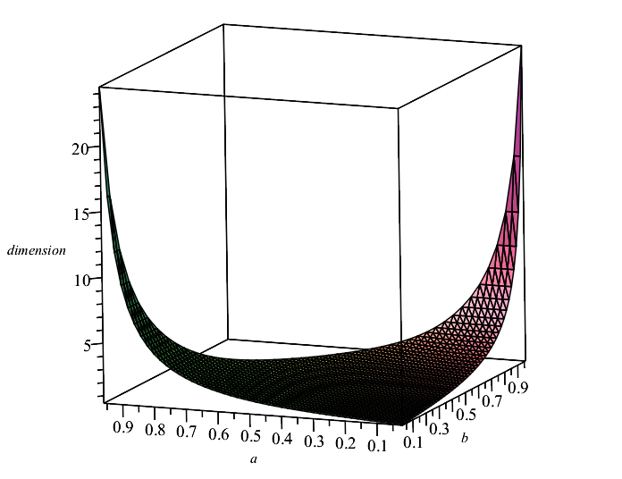
Figure 1. $\overline{\dim}_{\Phi}\mu$ as a function of $(a,b)$ for $\mu$ on $C_{ab}$ with $p\sim U[0,1]$.

It is notable that the dimension is a continuous function of $(a,b)\in\Lambda$ and it appears to increase as either $a\to 1$ or $b\to 1$ and vanish as $a$ and $b$ both tend to $0$. In fact that is indeed the case as we now argue.

For our discussion, let $D_{ab}$ be the almost sure upper $\Phi$-dimension of the random measure $\mu$ for the large $\Phi$ case. What we wish to show is that $D_{ab}\rightarrow 0$ as $a$ and $b$ tend to $0$ and $D_{ab}\rightarrow\infty$ as $a$ or $b$ tend to $1$.

Proof.

From (4.9) we have

$$G(\theta)=\frac{a^{\theta}\log\left(\frac{a^{\theta}}{a^{\theta}+b^{\theta}}\right)-a^{\theta}+b^{\theta}\log\left(\frac{b^{\theta}}{a^{\theta}+b^{\theta}}\right)-b^{\theta}}{a^{\theta}\log a+b^{\theta}\log b}.$$

and thus $G(\theta)\geq\theta$ if and only if

(4.10) $$a^{\theta}\log\left(\frac{a^{\theta}}{a^{\theta}+b^{\theta}}\right)-a^{\theta}+b^{\theta}\log\left(\frac{b^{\theta}}{a^{\theta}+b^{\theta}}\right)-b^{\theta}\leq\theta(a^{\theta}\log a+b^{\theta}\log b).$$

After some simplification, we see that this happens precisely when

$$(a^{\theta}+b^{\theta})(1+\log(a^{\theta}+b^{\theta}))\geq 0$$

which, since $a^{\theta}+b^{\theta}>0$, is equivalent to

$$a^{\theta}+b^{\theta}\geq e^{-1}.$$

Suppose $\theta<\infty$. Then this inequality will clearly hold once either $a$ or $b$ is sufficiently close to $1$. Consequently, Theorem 1(ii) implies $D_{ab}\geq\theta$ if either $a$ or $b$ is sufficiently large. Since $\theta$ was arbitrary, it follows that $D_{ab}$ tends to infinity as either $a$ or $b$ tend to $1$.

On the other hand, if $\theta>0$ and $a,b$ are both sufficiently small, then $a^{\theta}+b^{\theta}<e^{-1}$ and hence $G(\theta)<\theta$. Consequently, Theorem 1(i) implies that $D_{ab}<\theta$ and hence $D_{ab}\rightarrow 0$ as both $a,b\rightarrow 0$. ∎

4.4.2. $p_{n}$ chosen from the two-element set $\{p,1-p\}$ for fixed $0<p<1/2$

For our last example, we consider the deterministic Moran set $C_{ab}$, but with $p_{n}$ chosen from a two-element set.

Example 3.

Consider the deterministic Moran set $C_{ab}$ with $a<b$, but in this case let $\mu$ be the random measure with probability $p_{n}$ chosen uniformly from the two values $p$ or $1-p$ where $0<p<1/2$ is fixed. Define $\beta$ and $\eta$ by $a^{\beta}=b$ and $(1-p)^{\eta}=p,$ so $\beta<1$ and $\eta>1$. We claim

(4.11) $$\overline{\dim}_{\Phi}\mu_{\omega}=\left\{\begin{array}[]{cc}\frac{\log p+\log(1-p)}{2\log b}&\text{if }\eta+1+\beta-3\eta\beta\geq 0\\ \frac{\log p}{\frac{1}{2}(\log a+\log b)}&\text{if }\eta+1+\beta-3\eta\beta<0\end{array}\right.\text{ a.s}.$$

Proof.

Let $c(\theta)=a^{\theta}/(a^{\theta}+b^{\theta})$. Note that $c(\theta)$ is a decreasing function and for $\theta\geq 0,$ $c(\theta)\leq 1/2$. In particular, there is no non-negative solution to $c(\theta)=1-p>1/2$. Let $\theta_{0}$ satisfy $c(\theta_{0})=p$, so

$$\theta_{0}=\frac{\log((1-p)/p)}{\log(b/a)}=\frac{(\eta-1)\log(1-p)}{(1-\beta)\log a}.$$

If $\theta\geq\theta_{0},$ then both $p,1-p\geq c(\theta),$ so $Y_{n}=\log(1-p_{n})$ and $Z_{n}=\log b$.

If $0\leq\theta<\theta_{0},$ then $p\leq c(\theta)<1-p,$ hence if $p_{n}=p,$ then $Y_{n}=\log p_{n}=\log p$ and $Z_{n}=\log a$, while if $p_{n}=1-p,$ then $Y_{n}=\log(1-p_{n})=\log p$ and $Z_{n}=\log b$.

It is easy to see from these observations that

$$\mathbb{E}(Y_{1})=\left\{\begin{array}[]{cc}\frac{1}{2}(\log p+\log(1-p))&\text{if }\theta\geq\theta_{0}\\ \log p&\text{if }0\leq\theta<\theta_{0}\end{array}\right.$$

and

$$\mathbb{E}(Z_{1})=\left\{\begin{array}[]{cc}\log b&\text{if }\theta\geq\theta_{0}\\ \frac{1}{2}(\log a+\log b)&\text{if }0\leq\theta<\theta_{0}\end{array}\right..$$

Hence

$$G(\theta)=\left\{\begin{array}[]{cc}\frac{\log p+\log(1-p)}{2\log b}&\text{if }\theta\geq\theta_{0}\\ \frac{\log p}{\frac{1}{2}(\log a+\log b)}&\text{if }0\leq\theta<\theta_{0}\end{array}\right..$$

Replacing $p$ by $(1-p)^{\eta}$ and $b$ by $a^{\beta},$ this is the same as stating

$$G(\theta)=\left\{\begin{array}[]{cc}\frac{(\eta+1)\log(1-p)}{2\beta\log a}&\text{if }\theta\geq\frac{(\eta-1)\log(1-p)}{(1-\beta)\log a}\\ \frac{\eta\log(1-p)}{\frac{1}{2}(\beta+1)\log a}&\text{if }0\leq\theta<\frac{(\eta-1)\log(1-p)}{(1-\beta)\log a}\end{array}\right..$$

It is easy to check that if $\eta+1+\beta-3\eta\beta<0,$ then

$$\frac{\eta\log(1-p)}{\frac{1}{2}(1+\beta)\log a}<\frac{(\eta-1)\log(1-p)}{(1-\beta)\log a},$$

so $G(\alpha)=\alpha$ for

$$\alpha=\frac{\eta\log(1-p)}{\frac{1}{2}(\beta+1)\log a}=\frac{\log p}{\frac{1}{2}(\log a+\log b)}.$$

If $\alpha<\psi<\theta_{0},$ then obviously $G(\psi)=\alpha<\psi$. If $\psi\geq\theta_{0}>\alpha,$ then one can also check that $\eta+1+\beta-3\eta\beta<0$ implies

$$\frac{(\eta+1)\log(1-p)}{2\beta\log a}<\frac{\eta\log(1-p)}{\frac{1}{2}(\beta+1)\log a},$$

so again we have $G(\psi)<\alpha<\psi$.

Similarly, if $\eta+1+\beta-3\eta\beta\geq 0,$ then

$$\frac{(\eta+1)\log(1-p)}{2\beta\log a}\geq\frac{(\eta-1)\log(1-p)}{(1-\beta)\log a},$$

hence $G(\alpha)=\alpha$ for

$$\alpha=\frac{(\eta+1)\log(1-p)}{2\beta\log a}=\frac{\log p+\log(1-p)}{2\log b}$$

and if $\psi>\alpha,$ then $G(\psi)=\alpha<\psi$.

It follows from the theorem that $\overline{\dim}_{\Phi}\mu$ is as claimed in (4.11). ∎

4.4.3. Remarks on $G(\theta)$

For a fixed $A,B$ with $0<A<B<1$, set

$$\Lambda=(0,1)\times\{(a,b):A\leq\min\{a,b\}\leq a+b\leq B\}$$

as our parameter space. Then each (fixed) point $(p,a,b)\in\Lambda$ defines an iterated function system with probabilities (IFSP). Since this configuration (scalings $a,b$ and probabilities $p,1-p$) is chosen at every level, the resulting (deterministic) Moran set and measure is self-similar. The associated function $G(\theta)$ is piecewise constant with at most one discontinuity. It is possible to show that the location of the discontinuity cannot be between the two values of $G(\theta)$. Using this it is not difficult to see that there is a unique solution to $G(\theta)=\theta$.

In terms of our random model we can identify this single IFSP with a probability measure on $\Lambda$ which is a point-mass at the point $(p,a,b)$. If, instead, we take a probability measure on $\Lambda$ which is a combination of $N$ point masses, this is identified with a finite collection of different IFSPs to randomly choose from independently at each level. This time the function $G(\theta)$ has at most $N$ points of discontinuity and hence at most a finite number of solutions to $G(\theta)=\theta$. It would be very interesting to know if it were possible to construct an explicit example where $G(\theta)=\theta$ has no solutions; this would happen if a point of discontinuity of $G(\theta)$ coincided with a jump in the value from $G(\psi)>\psi$ to $G(\psi)<\psi$. For a single IFSP this is not possible, but it is unclear if this might be possible for a collection of IFSPs.

On the other hand if we begin with a probability measure $\eta$ on $\Lambda$ which is absolutely continuous with respect to Lebesgue measure, then $G(\theta)$ is a continuous function of $\theta$ and so Corollary 4 applies. It is worth pausing for a moment to contemplate why this is the case. For each fixed value of $\theta>0$, the set $\Lambda$ is partitioned into the two regions

$$\{p\leq\frac{a^{\theta}}{a^{\theta}+b^{\theta}}\}\quad\mbox{ and }\quad\{p>\frac{a^{\theta}}{a^{\theta}+b^{\theta}}\}$$

and the boundary between these regions is a smooth function of $(p,a,b)$ and also of $\theta$. The values of $Y(\theta)$ and $Z(\theta)$ depend entirely on which of these two sets the particular (random) choice of $(p,a,b)$ belongs to, and thus the expected values of $Y$ and $Z$ are given by the distribution of $\eta$ over these two sets. Since the boundary is a smooth surface, if $\eta$ is absolutely continuous, changing $\theta$ moves the boundary smoothly and thus changes $G(\theta)$ in a continuous way.

4.5. Comments on a more general construction

In this short subsection we briefly indicate how we can modify our construction so that it works in ${\mathbb{R}}^{D}$ and with the possibility of more than two children per parent. We can also allow the number of children at each level to be random and change from level to level. None of these significantly change anything as long as the number of children is uniformly bounded. To describe the generalization, we first need to establish some notation and definitions.

For $I\subset{\mathbb{R}}^{d}$, we denote by $diam(I)$ the diameter of $I$. Given $r>0$, we say $J\subseteq I$ is an $r$-similarity of $I$ if there is a similarity $S$ such that $J=S(I)$ and $diam(J)=r\cdot diam(I)$. A collection of $r_{j}$-similarities, $J_{1},J_{2},\ldots,J_{k}$, (possibly of $k$ distinct sizes) is $\tau$-separated if $d(J_{i},J_{j})\geq\tau\cdot diam(I)$ for all $i\neq j$. If such a collection exists, we say that $I$ has the $(k,\tau)$-separation property.

In the event that the interior of $I$ is non-empty, then for a given $k$ and small enough $\tau>0$, it is easy to see that $I$ will have the $(k,\tau)$-separation property for any $r_{j}\leq\rho_{k}$, $j=1,2,\ldots,k$, for a suitably small $\rho_{k}>0$. For example, if $I=[0,1]$ and $\tau k<1$, then $\rho_{k}=(1-(k-1)\tau)/k$ will work. We can view the $(k,\tau)$-separation condition as a uniform strong separation condition and is sometimes called the very strong separation condition.

Lemma 1, which relates balls with level $n$ sets and thus contains the essential geometric result, is changed very little in the more general setup. We redefine $L$ by the condition that

$$2B^{L-1}\leq\tau$$

and replace $1-B$ with $\tau$ in the proof and everything else is the same.

Let $I_{0}$ be a fixed compact subset of ${\mathbb{R}}^{D}$ with non-empty interior and diameter one. Fix $\tau\in(0,1)$, $K\geq 2$ and let $B_{i}\in(0,1)$, $i=2,\ldots,K$, be such that $I_{0}$ has the $(i,\tau)$-separation property for all $r_{j}\leq B_{i}$. We again let $A\in(0,\min_{i}B_{i})$. For each step $n$ in the construction, we take the random variables $K_{n}\in\{2,3,\ldots,K\}$ and $a_{n}^{(1)}(\omega),...,a_{n}^{(K_{n})}(\omega)$ where $a_{n}^{(j)}\geq A$ for each $j=1,2,\ldots,K_{n}$ and also $a_{n}^{(1)}+a_{n}^{(2)}+\cdots+a_{n}^{(K_{n})}\leq B_{K_{n}}$; these determine the relative sizes of the children at step $n$. Specifically, the children $J_{j}$ of the parent $I_{n}$ are $a_{n}^{(j)}$-similarities of $I_{n}$, for $j=1,2,\ldots,K_{n}$, which are $\tau$-separated. The random Moran set $C_{\omega}$ is then defined (as usual) to be

$$C_{\omega}=\bigcap_{n=1}^{\infty}{\mathcal{M}}_{n}(\omega),$$

where ${\mathcal{M}}_{n}(\omega)$ is the union of the step $n$ children.

Define a random measure $\mu_{\omega}$ supported on this Moran set $C_{\omega}$ by the rule that if the children of $I_{n}$ are labelled $I_{n}^{(j)}$, $j=1,...,K_{n}$, then $\mu_{\omega}(I_{n}^{(j)})=p_{n}^{(j)}$ $\mu_{\omega}(I_{n}),$ where the random variables $p_{n}^{(j)}(\omega)\geq 0$ satisfy $\sum_{j=1}^{K_{n}}p_{n}^{(j)}=1$ for all $n$. We assume that $\mathbb{E}(\left(a_{n}^{(j)}\right)^{-t})<\infty$ and $\mathbb{E}(\left(p_{n}^{(j)}\right)^{-t})<\infty$ for some $t>0$ and all $j=1,...,K_{n}$ and $n$.

Define

$$\begin{array}[]{c}Y_{n}(\theta)(\omega)=\log p_{n}^{(m)}(\omega)\\ Z_{n}(\theta)(\omega)=\log a_{n}^{(m)}(\omega)\end{array}\text{ if }\frac{a_{n}^{(m)\theta}}{p_{n}^{(m)}}=\max\left(\frac{a_{n}^{(k)\theta}}{p_{n}^{(k)}}:k=1,...,K_{n}\right)$$

and, as before, define

$$G(\theta)=\frac{\mathbb{E}_{\omega}(Y_{1}(\theta)(\omega))}{\mathbb{E}_{\omega}(Z_{1}(\theta)(\omega))}.$$

Essentially the same arguments as before show that Theorem 1 holds in this case as well.

Example 4.

Suppose $K_{n}=3$ (the same for all $n$) and the ratios are $a_{n}^{(1)}=1/4,$ $a_{n}^{(2)}=a_{n}^{(3)}=1/16$ for all $\omega$. Assume the probabilities $p_{n}^{(j)}$ are $1/2,1/4,1/4$ with $1/2$ assigned to position $j$ with equal likelihood. Note that if $p_{n}^{(1)}=1/2,$ then $\max\left(a_{n}^{(k)\theta}/p_{n}^{(k)}\right)=a_{n}^{(1)\theta}/p_{n}^{(1)}$ if $\theta\geq 1/2$ and $a_{n}^{(2)\theta}/p_{n}^{(2)}$ otherwise. If $p_{n}^{(j)}=1/2$ for $j=2,3,$ then $\max\left(a_{n}^{(k)\theta}/p_{n}^{(k)}\right)=a_{n}^{(1)\theta}/p_{n}^{(1)}$ for all $\theta\geq 0$. One can check that

$$\mathbb{E}(Y_{1}(\theta))=\left\{\begin{array}[]{cc}\log(1/4)&\text{if }\theta<1/2\\ \frac{5}{3}\log(1/2)&\text{ if }\theta\geq 1/2\end{array}\right.$$

and

$$\mathbb{E}(Z_{1}(\theta))=\left\{\begin{array}[]{cc}\frac{4}{3}\log(1/4)&\text{if }\theta<1/2\\ \log(1/4)&\text{ if }\theta\geq 1/2\end{array}\right..$$

Thus

$$G\mathbb{(}\theta)=\left\{\begin{array}[]{cc}3/4&\text{if }\theta<1/2\\ 5/6&\text{ if }\theta\geq 1/2\end{array}\right.$$

and consequently, for all large dimension functions $\Phi$, $\overline{\dim}_{\Phi}\mu=5/6$ a.s.

5.
Dimension results for small $\Phi$

We now move to a discussion of the “small” dimension functions $\Phi$. Recall that this means that $\Phi\ll\log\left|\log t\right|/\left|\log t\right|$. We again restrict our discussion to the case of two children per parent interval for the sake of clarity. The modifications necessary for the more general case are straightforward.

We introduce some further notation. Let

$$a_{0} = \text{ ess inf }a_{1}(\omega)\text{, }b_{0}=\text{ ess inf }b_{1}(\omega)\text{, }A_{0}=\text{ ess sup }a_{1}(\omega)\text{, }B_{0}=\text{ ess sup }b_{1}(\omega),$$

$$p_{0} = \text{ ess sup }p_{1}(\omega)\text{, }q_{0}=\text{ ess sup }(1-p_{1}(\omega))\text{, }P_{0}=\text{ ess inf }p_{1}(\omega)\text{, }Q_{0}=\text{ ess inf }(1-p_{1}(\omega)).$$

Note that $0<a_{0},b_{0},A_{0},B_{0}<1$ and $p_{0},q_{0}>0$. Put

$$\alpha=\max\left(\frac{\log P_{0}}{\log A_{0}},\frac{\log Q_{0}}{\log B_{0}}\right)\text{, }\beta=\min\left(\frac{\log p_{0}}{\log a_{0}},\frac{\log q_{0}}{\log b_{0}}\right)$$

where we understand $\alpha=\infty$ if either $P_{0}$ or $Q_{0}=0$.

Theorem 2.

There is a set $\Gamma$ of full measure, such that $\overline{\dim}_{\Phi}\mu_{\omega}=\alpha$ and $\underline{\dim}_{\Phi}\mu_{\omega}=\beta$ for all $\omega\in\Gamma$ and for all small dimension functions $\Phi$.

Proof.

We will begin by verifying that $\overline{\dim}_{\Phi}\mu\leq\alpha$ and $\underline{\dim}_{\Phi}\mu\geq\beta$ a.s. Consider the Moran interval $I_{v}=I_{v_{1}...v_{N}}$ and descendent interval $I_{u}=I_{v_{1}...v_{n}}$ where $\left|I_{u}\right|\leq\left|I_{v}\right|^{1+\Phi(\left|I_{v}\right|)}$. Then

$$\frac{\mu_{\omega}(I_{v})}{\mu_{\omega}(I_{u})}=\prod_{\begin{subarray}{c}j=N+1\\ v_{j}=0\end{subarray}}^{n}p_{j}^{-1}\prod_{\begin{subarray}{c}j=N+1\\ v_{j}=1\end{subarray}}^{n}(1-p_{j})^{-1}$$

and

$$\frac{\left|I_{v}\right|}{\left|I_{u}\right|}=\prod_{\begin{subarray}{c}j=N+1\\ v_{j}=0\end{subarray}}^{n}a_{j}^{-1}\prod_{\begin{subarray}{c}j=N+1\\ v_{j}=1\end{subarray}}^{n}b_{j}^{-1}.$$

Let

$$s_{N,n} = \#\{v_{j}=0:j=N+1,...,n\}\text{ and }$$

$$t_{N,n} = \#\{v_{j}=1:j=N+1,...,n\}\text{.}$$

With this notation, we have

$$p_{0}^{-s_{N,n}}q_{0}^{-t_{N,n}}\leq\frac{\mu_{\omega}(I_{v})}{\mu_{\omega}(I_{u})}\leq P_{0}^{-s_{N,n}}Q_{0}^{-t_{N,n}}$$

and

$$A_{0}^{-s_{N,n}}B_{0}^{-t_{N,n}}\leq\frac{\left|I_{v}\right|}{\left|I_{u}\right|}\leq a_{0}^{-s_{N,n}}b_{0}^{-t_{N,n}}.$$

Since we trivially have $\overline{\dim}_{\Phi}\mu_{\omega}\leq\infty,$ we can assume $\alpha<\infty$ and we remark that the definition of $\alpha$ ensures that $A_{0}^{-\alpha}\geq P_{0}^{-1}$, $B_{0}^{-\alpha}\geq Q_{0}^{-1}$. Thus, for almost all $\omega,$

$$\left(\frac{\left|I_{v}\right|}{\left|I_{u}\right|}\right)^{\alpha}\geq A_{0}^{-\alpha s_{N,n}}B_{0}^{-\alpha t_{N,n}}\geq P_{0}^{-s_{N,n}}Q_{0}^{-t_{N,n}}\geq\frac{\mu_{\omega}(I_{v})}{\mu_{\omega}(I_{u})}$$

Similarly, $a_{0}^{-\beta}\leq p_{0}^{-1}$, $b_{0}^{-\beta}\leq q_{0}^{-1},$ hence almost surely

$$\left(\frac{\left|I_{v}\right|}{\left|I_{u}\right|}\right)^{\beta}\leq a_{0}^{-\beta s_{N,n}}b_{0}^{-\beta t_{N,n}}\leq p_{0}^{-s_{N,n}}q_{0}^{-t_{N,n}}\leq\frac{\mu_{\omega}(I_{v})}{\mu_{\omega}(I_{u})}$$

Appealing to Lemma 2, it follows that there is a set of full measure such that $\overline{\dim}_{\Phi}\mu_{\omega}\leq\alpha$ and $\underline{\dim}_{\Phi}\mu_{\omega}\geq\beta$ for every $\omega$ in this set and any choice of (small) dimension function $\Phi$.

Now we establish the reverse inequalities. We will first see that for each $i\in\mathbb{N},$ there is a set $\Gamma_{i},$ of full measure, such that $\overline{\dim}_{\Phi}\mu_{\omega}\geq\alpha-1/i$ for every $\omega\in\Gamma_{i}$. Once this is established it will then follow that for every $\omega\in\Gamma=\bigcap_{i}\Gamma_{i},$ a set of full measure, $\overline{\dim}_{\Phi}\mu_{\omega}\geq\alpha$. Similar arguments will give the analogous result for the lower $\Phi$-dimensions.

First, suppose $P_{0},Q_{0}>0$. Without loss of generality, assume $\alpha=\log P_{0}/\log A_{0}$, so that $A_{0}^{-\alpha}=P_{0}^{-1}$ and $B_{0}^{-\alpha}\geq Q_{0}^{-1}$. As $A_{0}^{\alpha}=P_{0}$ and $A_{0}<1$, we can choose $\varepsilon_{i}>0$ so small that $(A_{0}-\varepsilon_{i})^{\alpha-1/i}/(P_{0}+\varepsilon_{i})>1$.

Because of the definition of $A_{0}$ and $P_{0},$ and the independence properties of the random variables, there is some $\delta_{i}=\delta_{i}(\varepsilon_{i})>0$ such that

$$\mathcal{P}(\,\max(\left|a_{1}(\omega)-A_{0}\right|,\left|p_{1}(\omega)-P_{0}\right|)<\varepsilon_{i}) =\hskip 122.85876pt$$

(5.1) $$\hskip 50.58878pt\mathcal{P(}\left|a_{1}(\omega)-A_{0}\right|<\varepsilon_{i})\mathcal{P(}\left|p_{1}(\omega)-P_{0}\right|<\varepsilon_{i}) \geq\delta_{i}.$$

Let

$$J_{i} :=\log B/(2\log\delta_{i}),$$

$$\chi_{N,i} :=\frac{J_{i}\log(N|\log A|)}{|\log B|}$$

and

$$\Phi_{i}(t)=\frac{J_{i}\log|\log t|}{|\log t|}.$$

Clearly, $\chi_{N,i}\rightarrow\infty$ as $N\rightarrow\infty$. Let

$$\Gamma_{N,i}=\left\{\omega:\max(\left|a_{j}(\omega)-A_{0}\right|,\left|p_{j}(\omega)-P_{0}\right|)<\varepsilon_{i}\text{ for }j=N+1,...,N+\chi_{N,i}\right\}.$$

Another independence argument shows

$$\mathcal{P}(\Gamma_{N,i})=\prod_{j=N+1}^{N+\chi_{N,i}}\mathcal{P(}\left|a_{j}(\omega)-A_{0}\right|<\varepsilon_{i})\mathcal{P(}\left|p_{j}(\omega)-P_{0}\right|<\varepsilon_{i})\geq\delta_{i}^{\chi_{N,i}}.$$

The choice of $J_{i}$ ensures that $\delta_{i}^{\chi_{N,i}}\geq 1/N$ for large enough $N$, thus if we let $N_{k}=k\log k,$ then for suitable $K_{0},$

$$\sum_{k}\mathcal{P}(\Gamma_{N_{k},i})\geq\sum_{k\geq K_{0}}\frac{1}{k\log k}=\infty.$$

We will assume $\delta_{i}>0$ is chosen sufficiently small so that $N_{k+1}>N_{k}+\chi_{N_{k},i}$. Hence the events $\{\Gamma_{N_{k},i}$ $\}_{k}$ are independent and the Borel Cantelli lemma implies that for each $i$, $\mathcal{P}(\Gamma_{N_{k},i}$ i.o.$)=1$. Let $\Gamma_{i}$ be this set of full measure.

Take any $\omega\in\Gamma_{i}$ and consider any Moran interval $I_{N},$ of step $N$. Let $I_{n}$ be the left-most descendent of $I_{N}$ at level $n=N+$ $\chi_{N,i}$. (We make the choice of the left descendent since $\alpha=\log P_{0}/\log A_{0}$.) Since $\left|I_{N}\right|\geq A^{N}$ and the function $t^{\Phi_{i}(t)}$ decreases as $t$ decreases to $0,$ the choice of $\chi_{N,i}$ ensures

$$\left|I_{N}\right|^{\Phi_{i}\left(\left|I_{N}\right|\right)}\geq A^{N\Phi_{i}(A^{N})}=A^{\frac{J_{i}\log(N\left|\log A\right|)}{\left|\log A\right|}}\geq B^{\chi_{N,i}}\geq\frac{\left|I_{n}\right|}{\left|I_{N}\right|}.$$

Hence $\left|I_{n}\right|\leq\left|I_{N}\right|^{1+\Phi_{i}\left(\left|I_{N}\right|\right)}$. As $\omega\in\Gamma_{i},$ it follows that for infinitely many $N,$

$$\frac{\mu_{\omega}(I_{N})}{\mu_{\omega}(I_{n})}=\left(\prod_{n=N+1}^{N+\chi_{N,i}}p_{n}\right)^{-1}\geq\left(P_{0}+\varepsilon\right)^{-\chi_{N,i}}$$

and

$$\left(\frac{\left|I_{N}\right|}{\left|I_{n}\right|}\right)^{\alpha-1/i}=\left(\prod_{i=N+1}^{N+\chi_{N,i}}a_{i}\right)^{-(\alpha-1/i)}\leq\left(A_{0}-\varepsilon\right)^{-(\alpha-1/i)\chi_{N,i}}.$$

But $\varepsilon_{i}$ was chosen so that $\left((A_{0}-\varepsilon_{i})^{\alpha-1/i}/(P_{0}+\varepsilon_{i})\right)^{M}\rightarrow\infty$ as $M\rightarrow\infty.$ Since $\chi_{N,i}\rightarrow\infty$ as $N\rightarrow\infty,$ it follows that there can be no constant $C$ such that

$$\frac{\mu_{\omega}(I_{N})}{\mu_{\omega}(I_{n})}\leq C\left(\frac{\left|I_{N}\right|}{\left|I_{n}\right|}\right)^{\alpha-1/i}$$

for all such $N,n$. By Lemma 2 that implies $\overline{\dim}_{\Phi_{i}}\mu_{\omega}\geq\alpha-1/i$ for all $\omega\in\Gamma_{i}$.

Let $\Gamma=\bigcap_{i=1}^{\infty}\Gamma_{i}$, a set of full measure, and assume $\Phi$ is any small dimension function. Then there is some function $H(t)\rightarrow 0$ as $t\rightarrow 0$ so that

$$\Phi(t)\leq\frac{H(t)\log|\log t|}{|\log t|}\text{ for all }t\leq t_{0}.$$

Consequently, for each $i$ there is some $t_{i}>0$ such that $\Phi(t)\leq\Phi_{i}(t)$ for all $t\leq t_{i}$. This property and our observations above ensure that $\overline{\dim}_{\Phi}\mu_{\omega}\geq$ $\overline{\dim}_{\Phi_{i}}\mu_{\omega}\geq\alpha-1/i$ for all $i$ and all $\omega\in\Gamma$. We conclude that $\overline{\dim}_{\Phi}\mu_{\omega}\geq\alpha$ for all $\omega\in\Gamma$, as we desired to show.

If, instead, $\alpha=\log Q_{0}/\log B_{0},$ we consider a Moran interval of level $N$ and its right-most descendent at level $N+\chi_{N,i}$ (for a suitable function $J_{i})$ and argue in a similar fashion.

The arguments to establish $\underline{\dim}_{\Phi}\mu\leq\beta$ a.s. are analogous, using the data $p_{0},q_{0},a_{0},b_{0},$ and left to the reader.

Since the values of $P_{0}$ and $Q_{0}$ are relevant only for the upper $\Phi$-dimension, to complete the proof in the case that either $P_{0}$ or $Q_{0}=0$ we only need establish that $\overline{\dim}_{\Phi}\mu_{\omega}=\alpha=\infty$ a.s.

Without loss of generality, assume $P_{0}=0$. Given $i\in\mathbb{N}$, choose $\varepsilon_{i}>0$ such that $\varepsilon_{i}(A_{0}-\varepsilon_{i})^{-i}<1,$ let $\delta_{i}=\delta(\varepsilon_{i})>0$ be as in (5.1) and define $J_{i},\Phi_{i}$, $\chi_{N,i},$ $\Gamma_{N,i},\Gamma_{i}$ as above. The same reasoning as before shows that $\overline{\dim}_{\Phi_{i}}\mu_{\omega}\geq i$ for all $\omega\in\Gamma_{i}$ and consequently for any small dimension function $\Phi,$ $\overline{\dim}_{\Phi}\mu_{\omega}=\infty$ for all $\omega\in\Gamma=\bigcap\Gamma_{i}$, a set of full measure. ∎

Corollary 5.

Almost surely, $\dim_{A}\mu_{\omega}=\alpha$ and $\dim_{L}\mu_{\omega}=\beta$.

Proof.

This is immediate from the theorem as the constant function $\Phi=0$ is a small dimension function. ∎

Example 5.

Consider, again, the Moran set $C_{ab}$ and random measure $\mu_{\omega}$ with probabilities chosen with equal likelihood from $\{p,1-p\}$ with $a<b$ and $p<1-p,$ as in Example 3. Then $\overline{\dim}_{\Phi}\mu_{\omega}=\log p/\log b$ and $\dim$${}_{\Phi}\mu_{\omega}=\log(1-p)/\log a$ almost surely.

Remark 2.

As in Subsection 4.5, suppose that each parent interval in the Moran set construction has $K\geq 2$ children and define a random Moran set $C_{\omega}$ and measure $\mu_{\omega}$ as was done there (with the same assumptions). With the notation of that subsection, for $j=1,...,K$ put

$$a^{(j)} = \text{ess inf }a_{1}^{(j)},A^{(j)}=\text{ess sup }a_{1}^{(j)}$$

$$p^{(j)} = \text{ess sup }p_{1}^{(j)},P^{(j)}=\text{ess inf }p_{1}^{(j)}$$

and let

$$\alpha=\max_{j=1,...,K}\left(\frac{\log P^{(j)}}{\log A^{(j)}}\right),\beta=\min_{j=1,...,K}\left(\frac{\log p^{(j)}}{\log a^{(j)}}\right).$$

The same reasoning as in the proof of the theorem shows $\overline{\dim}_{\Phi}\mu_{\omega}=\alpha$ and $\underline{\dim}_{\Phi}\mu_{\omega}=\beta$ for almost all $\omega$ and for all small dimension functions $\Phi$.

References

- [1] P. Assouad, Étude d’une dimension métrique liée à la possibilité de plongements dans n, C. R. Acad. Sci. Paris Sér. A-B, 288(1979), A731-A734.
- [2] M. Barnsley, J. Hutchinson and Ö. Stenflo, V-variable fractals: Fractals with partial self-similarity, Adv. Math., 218(2008), 2051-2088.
- [3] K. L. Chung, A course in probability theory, 3rd edition Academic Press, San Diego, 2001.
- [4] H. Chen, Y. Du and C. Wei, Quasi-lower dimension and quasi-Lipschitz mapping, Fractals, 25(2017), 1-9.
- [5] K. Falconer, Random fractals, Math. Proc. Camb. Phil. Soc., 100(1986), 559-582.
- [6] J. M. Fraser, Assouad dimension and fractal geometry, Cambridge Tracts in Mathematics 222, Camb. Univ. Press, 2020.
- [7] J. M. Fraser and D. Howroyd, On the upper regularity dimension of measures, Indiana Univ. Math. J., 69(2020), 685-712.
- [8] J. M. Fraser, J.-J. Miao and S. Troscheit, The Assouad dimension of randomly generated fractals, Ergodic Theory Dynam. Systems, 38(2018), 982-1011.
- [9] J. M. Fraser and S. Troscheit, Assouad spectrum of random self-affine carpets, Ergodic Theory Dynam. Systems, 41(2021), 2927-2945.
- [10] J. M. Fraser and H. Yu, New dimension spectra: finer information on scaling and homogeneity, Adv. Math., 329(2018), 273-328.
- [11] I. Garciá and K.E. Hare, Properties of quasi-Assouad dimension, Ann. Acad. Fennicae, 46 (2021), no. 1, 279-293.
- [12] I. Garciá, K.E. Hare and F. Mendivil, Intermediate Assouad-like dimensions, J. Fractal Geometry, 8(2021), no. 3, 201-245.
- [13] I. Garciá, K.E. Hare and F. Mendivil, Almost sure Assouad-like dimensions of complementary sets, Math. Z., 298(2021), no, 3-4, 1201-1220.
- [14] S. Graf, Statistically self-similar fractals, Prob. Theory Related Fields, 74(1987), 357-392.
- [15] K.E. Hare and K.G. Hare, Intermediate Assouad-like dimensions for measures, Fractals, 28(2020), no. 07, 205143.
- [16] K.E. Hare, K.G. Hare and S. Troscheit, Quasi-doubling of self-similar measures with overlaps, J. Fractal Geometry, 7(2020), 233-270.
- [17] K.E. Hare and F. Mendivil, Assouad dimensions of a class of random Moran measures. J. Math. Anal. Appl. 508(2022), no. 2, Paper No. 125912.
- [18] K.E. Hare and S. Troscheit, Lower Assouad dimension of measures and regularity, Camb. Phil. Soc., 170(2021), 379-415.
- [19] A. Käenmäki and J. Lehrbäck, Measures with predetermined regularity and inhomogeneous self-similar sets, Ark. Mat., 55(2017), 165–184.
- [20] A. Käenmäki, J. Lehrbäck and M. Vuorinen, Dimensions, Whitney covers, and tubular neighborhoods, Indiana Univ. Math. J., 62(2013), 1861–1889.
- [21] D.G. Larman, A new theory of dimension, Proc. Lond. Math. Soc., 3(1967), 178–192.
- [22] F. Lü and L. Xi, Quasi-Assouad dimension of fractals, J. Fractal Geom., 3(2016), 187-215.
- [23] V. Petrov, Limit theorems of probability theory: Sequences of independent random variables, Oxford Studies in Probability vol 4, Oxford, 1995.
- [24] S. Troscheit, The quasi-Assouad dimension for stochastically self-similar sets, Proc. Royal Soc. Edinburgh A, 150(2020), 261-275.
- [25] S. Troscheit, Assouad spectrum thresholds for some random constructions, Can. Math. Bull., 63(2020), 434-453.