Ensemble forecasts in reproducing kernel Hilbert space family

Benjamin Dufée Bérenger Hug Étienne Mémin Gilles Tissot INRIA/IRMAR Campus universitaire de Beaulieu, Rennes, 35042 Cedex, France
Abstract

A methodological framework for ensemble-based estimation and simulation of high dimensional dynamical systems such as the oceanic or atmospheric flows is proposed. To that end, the dynamical system is embedded in a family of reproducing kernel Hilbert spaces (RKHS) with kernel functions driven by the dynamics. In the RKHS family, the Koopman and Perron-Frobenius operators are unitary and uniformly continuous. This property warrants they can be expressed in exponential series of diagonalizable bounded evolution operators defined from their infinitesimal generators. Access to Lyapunov exponents and to exact ensemble based expressions of the tangent linear dynamics are directly available as well. The RKHS family enables us the devise of strikingly simple ensemble data assimilation methods for trajectory reconstructions in terms of constant-in-time linear combinations of trajectory samples. Such an embarrassingly simple strategy is made possible through a fully justified superposition principle ensuing from several fundamental theorems.

1 Introduction

Forecasting the state of geophysical fluids has become of paramount importance for our daily life either at short time scale, for weather prediction, or at long time scale, for climate study. There is in particular a strong need to provide reliable likely scenarios for probabilistic forecasts and uncertainty quantification. To that end, methods based on linear combinations of an ensemble of numerical simulations are becoming more and more ubiquitous. Ensemble forecasting and data assimilation techniques, where the linear coefficients are further constrained through partial observations of the system and Gaussian stochastic filtering strategies, are good examples developed in meteorological centers for weather forecast operational routine use. However, although efficient in practice, this linear superposition principle of solutions remains theoretically questionable for nonlinear dynamics. Very recently, such techniques have been further coupled with machine learning to characterize surrogate dynamical models from long time-series of observations. This includes neural networks, analog forecasting, reservoir computing, kernel methods to name only a few of the works of this wide emerging research effort [1, 2, 3, 4, 5, 6, 7, 8, 9, 10]. To characterize a surrogate model of the dynamics, these techniques are built upon principles such as delay coordinates embedding, empirical basis functions, or sparse linear representations. The difficulty here is to get sufficiently long data series to represent the manifold associated to a given observable of the system as well as to exhibit an intrinsic representation of the whole system that does not depend on parameters such as the discrete time-stepping, the integration time window, or the initial conditions. Looking for such intrinsic representation often leads to focus (at least theoretically) on reversible ergodic systems.

Spectral representation of the Koopman operator [11] or of its infinitesimal generator constitutes one of the most versatile approaches to achieve this objective as they enable in theory to extract intrinsic eigenfunctions of the system dynamics. Koopman operator or its dual, the Perron-Frobenious operator, have attracted a great deal of attention in the operator-theoretic branch of ergodic theory [12] as well as in data science for the study of data driven modeling of dynamical systems. Several techniques, starting from [13] and [14], have been proposed to estimate such spectral representation. Most of them rely either on longtime harmonic averages [14, 15, 16, 17] or on finite-dimensional approximations of the Koopman operator such as the dynamic modes representation and its extensions [18, 19, 20, 21, 22, 23, 24, 25, 26, 27, 28] or on Galerkin approximation and delay embedding [29, 30, 31]. See also the link between singular spectrum analysis (SSA) method [32], data-adaptive harmonic decomposition [33], Hankel alternative [29] and Koopman analysis [34, 35] for ergodic systems.

These methods enable performing spectral projection from long time series of measured observables of the system. The practical linear nature of the compositional Koopman operator, defined for any observable, $f$, of a dynamical system $\Phi_{t}(x)$ with initial condition $x$, as $(U_{t}f)(x):=f\circ\Phi_{t}(x)$, is nevertheless hindered by its infinite dimension. Due to this, it often exhibits a spectrum with a continuous component [36] and is not amenable to diagonalization nor to any sparsity assumption. Finite dimensional approximations and the direct use of matrix algebra numerical methods raises immediate questions on the pertinence of the associated estimation. To tackle these difficulties several techniques combining regularization, compactification of the generators, and reproducing kernel Hilbert space (RKHS) to work in spaces of smooth functions have been recently proposed [16, 17, 37]. They are possibly associated with forecast strategies [38, 39, 40] and transfer operator estimations [41, 42]. For data driven specification of dynamical systems RKHS or kernel methods have been also explored in a more direct way in terms of advanced Gaussian process regression techniques [43, 5, 44]. Kernel methods have been found particularly efficient in this context when coupled with a learning strategy for the kernel [6].

Working with RKHS brings convenient regular basis functions together with approximation convergence guaranties. However, the dynamical systems need still to be ergodic, and invertible to ensure that the Koopman operator has a simple point spectrum and an associated system of orthogonal basis eigenfunctions [12]. Measure invariance and invertibility warrants that the associated Koopman/Perron-Frobenius operators are dual unitary operators [12]. Note nevertheless that state-of-the-art estimation techniques based on Dynamic Mode Decomposition (DMD) or Hankel matrix [45, 29] require very long time series to converge to actual Koopman eigenvalues [34]. This is all the more detrimental for high-dimensional state-spaces. An extended dynamical modes decomposition has also been proposed to approximate the Koopman infinitesimal generator of deterministic or stochastic systems [46]. Like DMD, this approach corresponds to a direct discretization of the Koopman operator.

Recent reviews on modern Koopman analysis applications and their related algorithmic developments from measurements time series can be found in [47, 48, 49]. Another limitation is related to the definition of a kernel (and hence of a RKHS) independent of the dynamics to describe the system’s observable, which de facto boils down to the strong assumption of an invariance of the RKHS under the Koopman groups. This condition requires to define the RKHS from the subspace spanned by the Koopman operator eigenfunctions, which excludes in general classical parametric kernels. Note that in particular bias in the estimation of the Koopman eigenvalues have been observed for kernel-based methods based on finite dimensional approximation and sparsity assumptions [50, 51]. A technique coupling RKHS and the extended DMD approach of [46], enabling to provide an approximation of the Koopman generator, was proposed in [52]. In the same way as the previous techniques, an invariance of the RKHS is also assumed.

In this study we will explore the problem from a different angle. Instead of working with long time series of data, we will work with a set of realizations of a given dynamical system. The objective will be to learn this dynamics locally in the phase space to synthesize in a fast way new trajectories of the system through a theoretically well justified superposition principle. This superposition principle will in particular enable us to fully justify the linear combination assumption employed in many ensemble data assimilation filters even though the dynamics is nonlinear. To perform an efficient estimation inherently bound to the dynamics, we propose to embed the ensemble members in a set of time-evolving RKHS defining a family of spaces. This setting is designed to deal with large-scale systems such as oceanic or meteorological flows, for which it is out of the question to explore the whole attractor (if any), neither to run very long time simulations calibrated on real-world data of a likely transient system due to climate change. The present work relies on the fact that the kernel functions, usually called feature maps, between the native space and the RKHS family are transported by the dynamical system. This creates, at any time, an isometry between the evolving RKHS and the RKHS at a given initial time. Instead of being attached to a system state, the kernel is now fully associated with the dynamics and new ensemble members embedded in the RKHS family at a given time can be very simply forecast at a further time. For invertible dynamical systems, the Koopman and Perron-Frobenius operators in the RKHS family are unitary, like in $L^{2}$. However, they are in addition uniformly continuous, with bounded generators, and diagonalizable. As such they can be rigorously expanded in exponential form and their eigenfunctions provide an intrinsic orthonormal basis system related to the dynamics. This set of analytical properties immediately brings practical techniques to estimate Koopman eigenfunctions or essential features of the dynamics. Evaluations of these Koopman eigenfunctions at the ensemble members are directly available. Finite-time Lyapunov exponents associated with each Koopman eigenfunction are easily accessible on the RKHS family as well and can be used to get practical predictability time of the system. Expressions relating Koopman eigenfunctions to the tangent linear dynamics and its adjoint are also immediately available for data assimilation. These expressions, ensuing from the fundamental results listed previously, correspond in their simpler forms to the ensemble-based finite difference approximations intensively used in ensemble methods. Beyond that, the RKHS family finally leads to a theoretically well grounded superposition principle (for nonlinear dynamics) enabling the devise of embarrassingly simple methods for trajectory reconstructions in terms of constant-in-time linear combinations of trajectory samples.

The embedding of the trajectories in a time-evolving RKHS which follows the dynamical system can be related to concepts of local kernels [53], embedding in dynamical coordinates [54] or embedding of changing data over the parameter space as described in Coifman and Hirn [55]. In our case, we further exploit the relations with the Koopman operator together with an associated isometry, which allows us to define simple practical schemes for the setting of the time-evolving kernels and the modal information that can be extracted from them.

The main objective of this study is to propose a numerical framework for ensemble-based estimation and simulation of geophysical dynamics driven by systems of partial differential equations (PDE). In this study, we present theoretical elements for analyzing this framework. The mathematical assertions herein are based on idealized assumptions such as an infinite number of ensemble members, invertible dynamical systems and the availability of an ensemble of initial conditions. These theoretical statements will be further refined with more realistic assumptions in future works.

This paper is organized as follows. We start briefly recalling the definition and some properties of RKHS in the next section. These definitions are complemented by A which details and adapts several known results to our functional setting. The embedding of the Koopman and Perron-Frobenius operators in the RKHS family are then presented in sections 3 and 4. This is followed by the enunciation of our main results. The main theorems and properties are demonstrated in section 4 and in the appendixes. Numerical results for a quasi-geostrophic barotropic ocean model in an idealistic north Atlantic configuration will be presented in section 5 to support the pertinence of the proposed approach. This work corresponds to a presentation that has been given to the online seminar on Machine Learning for Dynamical Systems organized by the Turing institute (link).

2 Reproducing kernel Hilbert spaces

A RKHS, $\mathcal{H}$, is a Hilbert space of complex functions $f:E\mapsto\mathbb{C}$ defined over a non empty abstract set $E$ on which a positive definite kernel and a kernel-based inner product, $\langle\bm{\cdot}\,,\,\bm{\cdot}\rangle_{{\cal H}}$ can be defined. Throughout this work, we will consider that $E$ is a compact subset of a function vector space as we will work with an integral compact operator from which a convenient functional description can be set. In addition to enable the RKHS functions to be Gateaux differentiable, we will assume as in [56] that $E$ is defined as the closure of its nonempty interior, and we will work with RKHS defined from smooth enough kernels. RKHS possess remarkable properties, which make their use very appealing in statistical machine learning applications and interpolation problems [57, 58]. The kernels from which they are defined have a so called “reproducing property”.

Definition 1 (Reproducing kernel)

Let ${\cal H}$ be a Hilbert space of $\mathbb{C}$-valued functions defined on a non-empty compact topological space $E$. A map $k:E\times E\mapsto\mathbb{C}$ is called a reproducing kernel of ${\cal H}$ if it satisfies the following principal properties: $\forall x\in E,$

  • $\bullet$

    membership of the evaluation function $\;k(\bm{\cdot},x)\in{\cal H}$,

  • $\bullet$

    reproducing property $\forall f\in{\cal H},\;\bigl{\langle}f,k(\bm{\cdot},x)\bigr{\rangle}_{{\cal H}}=f(x)$.

The last property, provides an expression of the kernel as $k(x,y)=\overline{k(y,x)}=\bigl{\langle}k(\bm{\cdot},y),k(\bm{\cdot},x)\bigr{\rangle}_{{\cal H}}$, which is Hermitian – with $\overline{\bullet}$ denoting complex conjugate –, positive definite and associated with a continuous evaluation function $\delta_{x}f=\bigl{\langle}f,k(\bm{\cdot},x)\bigr{\rangle}_{{\cal H}}=f(x)$. The continuity of the Dirac evaluation operator is indeed sometimes taken as a definition of RKHS. By the Moore-Aronszajn theorem [59], the kernel $k$ defines uniquely the RKHS, ${\cal H}$, and vice versa. The set spanned by the feature maps ${\rm{Span}}\{k(\bm{\cdot},x),x\in E\}$, is dense in $({\cal H},\|\bm{\cdot}\|_{{\cal H}})$. We note also that useful kernel closure properties enable to define kernels through operations such as addition, Schur product, and function composition [57]. Besides, RKHS can be meaningfully characterized through integral operators, leading to an isometry with $L^{2}_{\mathbb{C}}(E,\nu)$ the space of square integrable functions defined on a compact metric space $E$ with finite measure $\nu$ [58].

Integral kernel operators

Let $k:E\times E\mapsto\mathbb{C}$ be $C^{(1,1)}(E\times E)$ (i.e. one time differentiable with respect to each argument), Hermitian, and positive definite, and let the map ${\cal L}_{k}:L_{\mathbb{C}}^{2}(E,\nu)\mapsto L_{\mathbb{C}}^{2}(E,\nu)$ be defined as:

$$\bigl{(}{\cal L}_{k}f\bigr{)}(x)=\int_{E}k(x,y)f(y)\,\nu({\mathrm{d}}y).$$ (1)

This operator, which must be understood within the composition with the continuous inclusion $i:C^{0}(E,\mathbb{C})\hookrightarrow L_{\mathbb{C}}^{2}(E,\nu)$, can be shown to be well defined, positive, compact and self-adjoint [58]. We will always assume that the space $L_{\mathbb{C}}^{2}(E,\nu)$ is infinite dimensional.The range of this operator is assumed to be dense in $L_{\mathbb{C}}^{2}(E,\nu)$ and hence infinite dimensional. From Mercer’s theorem [60], the feature maps $k(\bm{\cdot},x)$ span a RKHS defined through the eigenpairs $(\mu_{i},\varphi_{i})_{i\in\mathbb{N}}$ of the kernel $k$ :

$${\cal H}:=\bigl{\{}f\in L_{\mathbb{C}}^{2}(E,\nu),\;f=\displaystyle\sum_{i=0}^{\infty}a_{i}\varphi_{i}\;:\;\displaystyle\sum_{i}\dfrac{\,|a_{i}|^{2}}{\mu_{i}}<\infty\bigr{\}},$$ (2)

with no null eigenvalues and an inifinite sequence of eigenvalues since we have assumed that the kernel range is dense in $L_{\mathbb{C}}^{2}(E,\nu)$. The rank of the kernel (number of – non-zero – eigenvalues) corresponds to the dimension of ${\cal H}$, and will always be infinite in this work, which excludes the cases where $E$ is a finite set . The RKHS ${\cal H}$ is a space of smooth functions with decreasing high frequency coefficients. In fact, for all $u\in E$, there exists a constant $C>0$ for which $\|\partial_{u}f\|_{{L_{\mathbb{C}}^{2}(E,\nu)}}\leq C\,\left\|f\right\|_{{{\cal H}}}$ (Theorem 7A.2), where the derivative denotes the Gateau directional derivative of function $f$ in the direction $u$ defined as

$$\forall x,u\in E,\partial_{u}f{(x)}=\lim_{\epsilon\to 0}\frac{1}{\epsilon}\bigl{(}f(x+\epsilon u)-f(x)\bigr{)}.$$

In order to properly define the Gateaux derivative, a sufficient condition is to embed $E$ with a local vector space structure, which is for instance the case of differentiable manifolds. To enable such a differentiability property of the RKHS functions, we will in particular assume a weaker condition, namely that $E$ is the closure of its non empty interior [56]. We may also define uniquely a square-root symmetric isometric bijective operator ${\cal L}_{k}^{\scriptscriptstyle{1/2}}$ between $L_{\mathbb{C}}^{2}(E,\nu)$ and ${\cal H}$ (A.3). This operator enables to go from $L_{\mathbb{C}}^{2}(E,\nu)$ to ${\cal H}$ by increasing the functions regularity while its inverse lowers the function regularity by bringing them back to $L_{\mathbb{C}}^{2}(E,\nu)$. Both operators are bounded. The injection $j:{\cal H}\mapsto L^{2}_{\mathbb{C}}(E,\nu)$ is continuous and compact (Theorem 8A.3) and $j({\cal H})$ is assumed to be dense in $L_{\mathbb{C}}^{2}(E,\nu)$ (Prop. 11). These statements are precisely recalled in A.

Remark 1

As mentioned above, the spaces $\mathcal{H}$ and $L_{\mathbb{C}}^{2}(E,\nu)$ are infinite dimensional spaces, preventing $E$ to be a finite set. Note that the denseness and the infinite dimensionality assumptions can easily be relaxed – see Remark 16A.3.

3 Dynamical systems on a RKHS family

We consider an invertible nonsingular dynamical system $X(t)=\Phi_{t}(X_{0})$, defined from a continuous flow, $\Phi_{t}$ (meaning that, for any $X\in\Omega$, the mapping $t\mapsto\Phi_{t}(X)$ is continuous), on a compact invariant metric phase space differentiable manifold, $\Omega$, (i.e. $\Phi^{-1}_{t}(\Omega)=\Omega$, $\forall t\in\mathbb{R}^{+}$) of time evolving vector functions over a spatial support $\Omega_{x}$. The functions $X:\mathbb{R}^{+}\times\Omega_{x}\mapsto\mathbb{R}^{d}$ with $X\in C^{p}$, $p\geq 1$, are solutions of the following $d$-dimensional differential system:

$$\left\{\begin{aligned} \partial_{t}X(t,{\color[rgb]{0,0,0}\bm{\cdot}})&={\cal M}\bigl{(}X(t,{\color[rgb]{0,0,0}\bm{\cdot}})\bigr{)},\text{ with }X(t,{\color[rgb]{0,0,0}\bm{\cdot}})\in\Omega,\forall t>0,\\ X(0,{\color[rgb]{0,0,0}\bm{\cdot}})&=X_{0}({\color[rgb]{0,0,0}\bm{\cdot}}).\end{aligned}\right.$$ (3)

The nonlinear differential operator ${\cal M}{:\Omega\to\Omega}$ is assumed $C^{1}{(\Omega)}$, and in particular its linear tangent expression defined as the Gateaux derivative:

$$\partial_{X}{\cal M}(X)\delta X=\lim_{\beta\to 0}\frac{1}{\beta}\biggl{(}{\cal M}\bigl{(}X(t,{\color[rgb]{0,0,0}\bm{\cdot}})+\beta{\delta}X(t,{\color[rgb]{0,0,0}\bm{\cdot}})\bigr{)}-{\cal M}\bigl{(}X(t,{\color[rgb]{0,0,0}\bm{\cdot}})\bigr{)}\biggr{)}$$

is such that $\sup_{X\in\Omega}\partial_{X}{\cal M}(X)<\infty$ (since $\Omega$ is compact). Let us note that such a differentiablity assumption is quite common in geophysical flows, as otherwise so-called 4DVar variational assimilation strategies [61] derived from optimal control theory [62] and that are routinely used in weather and climate centers would make no sense. In the following, we consider the measure space $(\Omega_{x},\mathrm{d})$ where $\mathrm{d}$ is the Lebesgue measure on $\Omega_{x}$. We note $L^{2}(\Omega_{x},\mathbb{R}^{d}):=\{f=(f_{1},..,f_{d}):\Omega_{x}\mapsto\mathbb{R}^{d}\;:\;\text{for all}\;1\leq i\leq d\quad f_{i}\in L^{2}(\Omega_{x},\mathbb{R})\}$ the vector space of square integrable functions on $\Omega_{x}$. We note $\|\bm{\cdot}\|_{{L^{2}}}$ the norm associated with $L^{2}(\Omega_{x},\mathbb{R}^{d})$ and given by $\|f\|^{2}_{{L^{2}}}:=\sum_{i=1}^{d}\|f_{i}\|^{2}_{L^{2}(\Omega_{x},\mathbb{R})}$ for all $f\in L^{2}(\Omega_{x},\mathbb{R}^{d})$. The set $\Omega$ is included in $L^{2}(\Omega_{x},\mathbb{R}^{d})$. The system (3) is assumed to admit a finite invariant measure $\nu$ on $\Omega$ (note that from invertibility the measure is also nonsingular with $\nu(\Phi^{-1}_{t})(A)=0$, $\forall A{\subset}\Omega$ such that $\nu(A)=0$). The system’s observables are square integrable measurable complex functions with respect to measure $\nu$. They belong to the Hilbert space $L^{2}_{\mathbb{C}}(\Omega,\nu)$ with the inner product $\langle\bm{\cdot}\,,\,\bm{\cdot}\rangle_{{L^{2}_{\mathbb{C}}(\Omega,\nu)}}$ given for $f$ and $g\in L^{2}_{\mathbb{C}}(\Omega,\nu)$ by

$$\langle f\,,\,g\rangle_{{L^{2}_{\mathbb{C}}(\Omega,\nu)}}:=\int_{\Omega}f(y)\,\overline{\,g(y)\,}\;\nu(\mathrm{d}y).$$

Depending on the context $X(t,{\color[rgb]{0,0,0}\bm{\cdot}})$ or $X_{t}$ will denote either an element of $\Omega$ or the function ${\color[rgb]{0,0,0}X(t,\bm{\cdot})}\colon\Omega_{x}\mapsto\mathbb{R}^{d}$ such that $x\mapsto X(t,x)$.

In this work, the set of different initial conditions $\Omega_{0}$ is an infinite compact subset of $L^{2}(\Omega_{x},\mathbb{R}^{d})$. For all time $t\geq 0$, we denote by $\Omega_{t}\subset\Omega\subset L^{2}(\Omega_{x},\mathbb{R}^{d})$ the space defined as $\Omega_{t}:=\Phi_{t}(\Omega_{0})$. Furthermore, the set $\Omega_{0}$ of initial conditions will be assumed to be given – as it is usual in ensemble data assimilation or forecasting applications – and rich enough so that $\bigcup_{t\geq 0}(\Omega_{t})=\Omega$. Hence, by this, each point of the manifold, $\Omega$, is assumed to be uniquely characterized by a given initial condition and the integration of the invertible dynamical system over a given time $t$. In other words, for any $X\in\Omega$, there exists a unique initial condition $X_{0}\in\Omega_{0}$ and a unique time $t\in\mathbb{R}_{+}$ such that $X=\Phi_{t}(X_{0})$. All the points of the phase space are tagged with a reaching time. A stationary point belongs to all sets $\Omega_{t}$ and a recurrent point belongs also to several sets. All the sets $\Omega_{t}$ will be assumed to be compact subset of a functions vector space, defined as the closure of their non-empty interior. Compactness enables the use of a classical Mercer theorem while non-empty interior allows differentiability of the associated RKHS feature maps. Compactness could be relaxed with generalized form of the Mercer theorem [63, 64]. This is however outside of the scope of this paper and we will remain in the case of compactness assumption. Let us note that an assumption of finite dimensional vector spaces for the set $\Omega_{t}$ could have been done (which comes immediately by the Riesz theorem, if we additionally impose a vectorial space structure together with compactness and non-empty interior). While many geophysical systems are conjectured to have finite-dimensional attractors (like the 2D Navier-Stokes equations [65, 66]), we prefer to adhere to a more general assumption here.

Remark 2

For measure-preserving systems, the assumption $\Omega=\bigcup_{t\geq 0}\Omega_{t}$ is weaker than an ergodicity assumption, which is equivalent (together with Poincaré recurrence associated with measure preserving dynamical system) to the following statement [12] (Lemma 6.19): for any (non-empty) measurable set $A\subset\Omega$, then the set $\bigcup_{t\geq 0}\Phi^{-1}_{t}(A)=\Omega$. Ergodicity is very commonly assumed in the literature on Koopman spectral analysis [47]. We have here a weaker assumption.

Defining at each time $t$, from ensemble $\Omega_{t}$, a positive Hermitian kernel $k_{\Omega_{t}}:\Omega_{t}\times\Omega_{t}$, there exists a unique associated RKHS ${\cal H}_{t}$. In the following for the sake of concision the kernels $k_{\Omega_{t}}$, will be denoted by $k_{t}$ to refer to the dependence on the set $\Omega_{t}$. For all $t\geq 0$, we will use the notation $X_{t}=\Phi_{t}(X_{0})$ and $\left({\cal H}_{t},\langle\,\bm{\cdot}\,,\,\bm{\cdot}\,\rangle_{{\cal H}_{t}},\|\bm{\cdot}\|_{{}_{{\cal H}_{t}}}\right)$ for the RKHS associated with the kernel $k_{t}$ defined on $\Omega_{t}\times\Omega_{t}$. The kernels are assumed to be $C^{{\color[rgb]{0,0,0}(1,1)}}(\Omega_{t}\times\Omega_{t})$ and as a consequence as shown in appendix A, the associated feature maps have derivatives in ${\cal H}_{t}$. The RKHS ${\cal H}_{t}$ for all time $t\geq 0$ forms a family of Hilbert spaces of complex functions, each of them equipped with their own inner product $k_{t}(Y_{t},X_{t})$, for all functions $X_{t},Y_{t}\in$ $\Omega_{t}$. At any time, a measurable function of the system state, usually referred to as an observable, $f$, belonging to the RKHS ${\cal H}_{t}$ can be described as the limit of a linear combination of the feature maps $\{k_{t}(\bm{\cdot},X_{t}),X_{t}\in\Omega_{t}\}$. As it will be shown, the features maps of this RKHS family can be expressed on a time evolving orthonormal systems of basis functions, connected to each other through an exponential form and given by the eigenfunctions of the infinitesimal evolution operator of a “Koopman-like” operator defined on the RKHS family. The RKHS family is defined by ${\mathcal{W}}=({\cal H}_{t})_{t\geq 0}$. In the following, we shall present a summary of the mathematical results associated to the Koopman operator in the RKHS family .

Numerically, in practice, the setup is based on $n$ realizations (called ensemble members) of this dynamical system, $\{X^{(i)}_{t},i=1,\ldots,n\}$, generated from a finite set of different initial conditions $\{X^{(i)}_{0},i=1,\ldots,n\}\subset\Omega_{0}$, are available up to time $T$. Still, we underline that, in the following development, the time horizon can be infinite, the sets $\Omega_{t}$ are infinite and the corresponding RKHS $\mathcal{H}_{t}$ are infinite dimensional. This setting (both practically and theoretically) is quite common for ensemble methods applied to geophysical systems. The ensemble size is small in general, while the phase space is in theory infinite dimensional (or at least of very high dimension). In the same way as it is usual in data assimilation or climate/weather forecasting, the dynamics on which we will experiment our setting will be assume to be invertible at least on small time range. Although often derived from Euler equation, geophysical dynamics introduce in one way or the other some viscosity and are not stricto-sensu invertible. Additionally, for most of these systems, only local-in-time solutions have been demonstrated thus far. As demonstrated in the numerical section, the proposed framework yields good results for a simple geophysical PDEs system within a short-time range. As already mentioned in the introduction, the primary goal of this work is to establish a numerical framework for ensemble-based estimation and simulation. We provide below some theoretical elements for analyzing this framework. These mathematical statements rely in particular on the assumptions of an infinite number of members in the ensemble and on invertible dynamical systems, which is obviously not the case in practice. These theoretical statements will be refined with more realistic assumptions in subsequent works.

4 Koopman operator in the RKHS family

So far, we did not give any precise definition of the kernels associated to the RKHS family ${\cal H}_{t}$ yet. These kernels are defined from a known a priori initial kernel, $k_{0}:\Omega_{0}\times\Omega_{0}$, as:

Definition 1 (${\cal H}_{t}$ kernel)

The kernel $k_{t}$ associated to the RKHS ${\cal H}_{t}$ are defined as

$$\forall X_{t},Y_{t}\in\Omega_{t},\quad k_{t}\bigl{(}Y_{t}\,,\,X_{t}\bigr{)}=k_{0}\bigl{(}\Phi^{-1}_{t}(Y_{t})\,,\,\Phi^{-1}_{t}(X_{t})\bigr{)},$$ (4)

where $k_{0}:\Omega_{0}\times\Omega_{0}$ is a given kernel.

These kernels can also be equivalently defined introducing the operators, ${\cal U}_{t}$, operating on the feature maps. An isometric property of this operator on the RKHS family, enables us to fully define the kernels along time in the same way as the previous definition. The operator ${\cal U}_{t}:{\cal H}_{0}\mapsto{\cal H}_{t}$ defined such that

$${\cal U}_{t}k_{0}(\bm{\cdot},X_{0})=k_{t}\bigl{(}\bm{\cdot},\Phi_{t}(X_{0})\bigr{)},$$ (5)

transports the kernel feature maps on the RKHS family by composition with the system’s dynamics. This operator, and more specifically an associated infinitesimal evolution operator, will enable us to define the feature maps of ${\cal H}_{t}$ from an initial set of feature maps on ${\cal H}_{0}$. As will be fully detailed in section 4.1, we will see that the operator ${\cal U}_{t}$ is indeed directly related to the restriction on ${\cal H}_{t}$ of the adjoint of the Koopman operator $U_{t}$ on a bigger RKHS space, ${\cal H}$, associated to a fixed kernel defined on the whole phase space, $\Omega$. As ${\cal U}_{t}$ propagates forward the second argument of the feature maps, it is referred in the following to as the Koopman kernel operator in the RKHS family. Indeed, it will be pointed out that, for any $f\in{\cal H}$, and any $X_{0}\in\Omega_{0}$,

$\displaystyle U_{t}f(X_{0})=f(X_{t})$ $\displaystyle=\bigl{\langle}R_{t}f\,,\,k_{t}(\bm{\cdot}\,,\,X_{t})\bigr{\rangle}_{{\cal H}_{t}}$
$\displaystyle=\bigl{\langle}R_{t}f\,,\,{\cal U}_{t}k_{0}(\bm{\cdot}\,,\,X_{0})\bigr{\rangle}_{{\cal H}_{t}},$

where $U_{t}$ denotes the Koopman operator operating on $L^{2}_{\mathbb{C}}(\Omega,\nu)$, and $R_{t}f$ denotes the restriction of $f$ to $\Omega_{t}\subset\Omega$. This expression exhibits a kernel expression of the Koopman operator definition and formally, at this point, the operator ${\cal U}_{t}$ can be thought as a kernel expression of the Koopman operator.

The global kernel $k$ (respectively the associated RKHS) is tightly bound to the time evolving kernels $k_{t}$ (respectively $({\cal H}_{t})_{t\geq 0}$). The restriction on ${\cal H}$ of the Koopman operator $U_{t}$ and its adjoint the Perron-Frobenius $P_{t}$ exhibit some remarkable properties. As classically, the operators $U_{t}$ and $P_{t}$ are unitary in $L^{2}_{\mathbb{C}}(\Omega,\nu)$ (Prop. 1), but they have the striking property to be uniformly continuous in $L^{2}_{\mathbb{C}}(\Omega,\nu)$ (i.e. with bounded generators – Theorem 2). As such, they can be expanded in an uniformly converging exponential series. Nevertheless, it must be outlined that the fixed kernel $k(x,y)$ and consequently ${\cal H}$ are in practice only partially accessible as they are defined on the whole manifold of the dynamics and such expansion cannot be directly used. A local representation of the RKHS family ${\mathcal{W}}$ is on the other hand much easier to infer in practice through the time evolution of ensembles $\Omega_{t}$ and kernels $k_{t}$. As we shall see, the operator ${\cal U}_{t}$ on ${\mathcal{W}}$ inherits many properties from $U_{t}$ and in particular, a related form of exponential series expansion (Theorem 1).

The Koopman kernel operator in the RKHS family, ${\cal U}_{t}$, defines an isometry from ${\cal H}_{0}$ to ${\cal H}_{t}$ (Theorem 3)

$\displaystyle\biggl{\langle}k_{t}\bigl{(}\bm{\cdot},\!\Phi_{t}(Y_{0})\bigr{)},k_{t}\bigl{(}\bm{\cdot},\!\Phi_{t}(X_{0})\bigr{)}\biggr{\rangle}_{\!\!{\cal H}_{t}}\!\!$ $\displaystyle=\!\biggl{\langle}k_{0}\bigl{(}\bm{\cdot},\!Y_{0}\bigr{)},k_{0}\bigl{(}\bm{\cdot},\!X_{0}\bigr{)}\biggr{\rangle}_{\!\!{\cal H}_{0}},$ (6)
$\displaystyle k_{t}\bigl{(}\Phi_{t}(X_{0}),\Phi_{t}(Y_{0})\bigr{)}\!$ $\displaystyle=\!k_{0}(X_{0},Y_{0}).$

This isometry ensues obviously directly from definition 1. But, it can be also guessed from definition (5) and the unitarity of ${\cal U}_{t}$ (Theorem 3, Prop.6), inherited from the unitarity in $L^{2}_{\mathbb{C}}(\Omega,\nu)$ of the Koopman operator and of its adjoint, the Perron-Frobenious operator. This property is of major practical interest as it allows us to define the kernels of the RKHS family from a given initial kernel fixed by the user. The kernels remain constant along the system trajectories. Alternatively, an explicit form of the feature maps can be obtained from an adjoint transport equation associated to an evolution operator in the RKHS family. Nevertheless, the isometry is far more straightforward to use to set the kernel evolution. This isometry will reveal also very useful for the data assimilation and trajectories reconstruction problems investigated in section 5. Strikingly, we have even more than this kernel isometry. An evolution operator $A_{U\!,\,t}:{\cal H}_{t}\to L_{\mathbb{C}}^{2}(\Omega_{t},\nu)$, associated to the infinitesimal generator of Koopman operator $U_{t}$ can also be defined as

$$A_{U\!,\,t}\;k_{t}(\bm{\cdot},X_{t}):=\partial_{{\cal M}(\bm{\cdot})}\,k_{t}(\bm{\cdot},X_{t}),$$ (7)

where $\partial_{u}k_{t}(\bm{\cdot},X_{t})$ stands for the Gateaux directional derivative along $u\in\Omega$ of function $k(\bm{\cdot},X_{t})$. This operator that will be shown to be bounded (Prop.7) and skew-symmetric (Prop.8) for the inner product of $L^{2}_{\mathbb{C}}(\Omega,\nu)$ plays the role of an infinitesimal generator on ${\cal W}$ and enables us expressing an exponential expansion of ${\cal U}_{t}$.

Theorem 1 (The RKHS family spectral representation)

Let $\Omega$ be a compact metric differentiable manifold that is invariant by an invertible continuous flow, $\Phi_{t}$, defined from a dynamical system (3) admitting an invariant finite measure $\nu$ on $\Omega$. Let $\Omega_{0}\subset\Omega$ be an infinite compact subset of initial conditions and define $\Omega_{t}=\Phi_{t}(\Omega_{0})$, with the assumption that $\Omega=\bigcup_{t\geq 0}\Omega_{t}$. Consider a $C^{(1,1)}$ initial kernel $k_{0}:\Omega_{0}\times\Omega_{0}\rightarrow\mathbb{C}$ that uniquely defines an infinite dimensional initial RKHS $\mathcal{H}_{0}$, and, the time dependent kernels $k_{t}$ defined in (4) together with its associated RKHS family ${\mathcal{W}}=({\cal H}_{t})_{t\geq 0}$. Then, the evolution operator $A_{U\!,\,t}:{\cal H}_{t}\mapsto L_{\mathbb{C}}^{2}(\Omega_{t},\nu)$ given in (7), and which is defined from the restriction of the infinitesimal generator $A_{U}$ of the Koopman operator in $L_{\mathbb{C}}^{2}(\Omega,\nu)$, can be diagonalized, at any time $t\geq 0$, by an orthonormal basis $(\psi^{t}_{\ell})_{\ell}$ of ${\cal H}_{t}$ such that

$$A_{U\!,\,t}\psi^{\,t}_{\ell}(X_{t})=\lambda_{\ell}{{j\circ}}\psi^{\,t}_{\ell}(X_{t}),$$

where $j$ is the injection $j:{\cal H}_{t}\mapsto L^{2}_{\mathbb{C}}(\Omega_{t},\nu)$. We have in addition the following relation between the orthonormal basis systems along time:

$$\forall t\geq 0\;\;\psi^{\,t}_{\ell}(X_{t})=\exp(t\;\lambda_{\ell})\psi^{0}_{\ell}(X_{0}),$$ (8)

with $X_{t}=\Phi_{t}(X_{0})$. Furthermore, the purely imaginary eigenvalues $(\lambda_{\ell})_{\ell}$ do not depend on time.

This theorem, which constitutes our main result, provides us a time-evolving system of orthonormal bases of the RKHS family. It brings us the capability to express any observable of the system in terms of bases that are intrinsically linked to the dynamics and related to each other by an exponential relation. The eigenvalues of $A_{U\!,\,t}$ are purely imaginary since this operator is skew-symmetric in $L^{2}_{\mathbb{C}}(\Omega_{t},\nu)$. Remarkably, the eigenvalues of each $A_{U\!,\,t}$ do not depend on time and are connected with the same covariant eigenfunctions (in the sense of (8)). These eigenfunctions correspond to restrictions of eigenfunctions of the infinitesimal generator of Koopman/Perron-Frobenius operators defined on ${\cal H}$. The proofs of these results are fully detailed in the next section.

The frozen in time spectrum, also referred to as iso-spectral property in the litterature, connects directly the RKHS family representation with Lax pair theory of integrable system [67]. Here the Lax pair is provided by the operator $A_{U\!,\,t}$ at a given time and the evolution equation (8). The expression of the dynamical system in the RKHS family (i.e. through the feature maps) provides a compatility condition for the Lax pair. As the existence of a Lax pair is directly related to integrable systems, it means that the the RKHS family representation formally retains only the integrable part of a (non-necessary integrable) dynamical system. This relation between Koopman operator and integrable systems has been already put forward in several works [47, 68]. Here an ensemble characterization of such a relation is exhibited.

The kernel isometry (6) (Theorem 3) and the Koopman spectral representation in the RKHS family (Theorem 1) constitute fundamental results enabling us to build very simple ensemble-based trajectory reconstructions for new initial conditions without the requirement of resimulating the dynamical system. Amazingly, the family of RKHS together with the Koopman isometry allows to define a system’s trajectory as a constant-in-time linear combination of the time varying RKHS feature maps. Several of such reconstruction techniques, based on this fully justified superposition principle, will be shown in section 5. We will in particular demonstrate the potential of this framework with a simple and very cheap data assimilation technique in the context of very scarce data in space and time. In the next section we demonstrate the different properties related to the RKHS family.

4.1 Proofs on the properties of the Koopman operator in the RKHS family and of the the RKHS family spectral theorem

As explained in the previous section the RKHS family, $\bigl{(}{\cal H}_{t}\bigr{)}_{t\geq 0}$, does not have a good topology to work with. We need first to start defining a “big” set with a better topology and which encompasses all the RKHS ${\cal H}_{t}$. On this big encompassing set, we shall then define a Koopman operator enabling us to study properly the Koopman operator in the RKHS family.

4.1.1 Construction of the “big” encompassing set ${\cal H}$

The phase space $\Omega$ corresponds to the set generated by the value of the dynamical system at a given time $t$. We note hence that $\Omega_{t}$ is a subset of $\Omega$. Each point of $\Omega$ designates a phase-space point $X=\Phi_{t}(X_{0})$ uniquely defined from time $t$ and initial condition $X_{0}\in\Omega_{0}$. In order to define the RKHS ${\cal H}$, let us define from the kernel $k_{t}:\Omega_{t}\times\Omega_{t}$ a symmetric positive definite map $k:\Omega\times\Omega$.

Definition 2 (${\cal H}$ kernel)

For all $X=\Phi_{r}(X_{0}),\,Y=\Phi_{s}(Y_{0})\in\Omega$, with $X_{0},\,Y_{0}\in\Omega_{0}$ we define

$$k(X\,,\,Y)=k_{0}\bigl{(}X_{0}\,,\,Y_{0}\bigr{)}\ell(r,s)=k_{t}\bigl{(}\Phi_{t}(X_{0})\,,\,\Phi_{t}(Y_{0})\bigr{)}\ell(r,s)\quad\forall t\geq 0,$$ (9)

where $\ell:\mathbb{R}_{+}\times\mathbb{R}_{+}\to\mathbb{R}$ is a symmetric kernel defined, for all $r,s\in\mathbb{R}{{}^{+}}$ by

$$\ell(r,s)=\varphi(r-s),$$ (10)

where $\varphi$ is a twice-differentiable even positive definite function such that $\varphi(0)=1$.

The positivity and symmetry of kernel $k$ ensues from the property of kernels $k_{0}$ and $\ell$, which are assumed to be valid kernels. Kernel $k$ inherits the regularity conditions of $k_{0}$ and $\ell$ and is $C^{{\color[rgb]{0,0,0}(1,1)}}(\Omega\times\Omega)$ as well. In the trivial case where $\varphi=1$, then comparing any pair of points on two trajectories would be equivalent to compare the initial conditions, which would result in a quite poor kernel, and degeneracy issues. In order to enrich the kernel structure, one can think of $\varphi$ as a regularized Dirac distribution, or a time Gaussian distribution, that will discriminate the points of the phase space that are reached at different times.

By the Moore-Aronszajn theorem, there exists a unique RKHS called $\left({\cal H},\langle\,\bm{\cdot}\,,\,\bm{\cdot}\,\rangle_{{\cal H}},\|\bm{\cdot}\|_{{}_{{\cal H}}}\right)$ with kernel $k$. We note that in practice the full knowledge of the phase-space is completely unreachable. Again, we therefore stress the fact that the setting of this encompassing RKHS ${\cal H}$ has only a theoretical purpose. The RKHS ${\cal H}$ can be connected to each RKHS of the family ${\mathcal{W}}$ through extension and restriction operators denoted $E_{t}$ and $R_{t}$ respectively, and defined as follows. For all $t\geq 0$, let

$$\begin{array}[]{ccccc}E_{t}:&&{\cal H}_{t}&\to&{\cal H}\\ &&k_{t}(\,\bm{\cdot}\,,X_{t})&\mapsto&\;k(\,\bm{\cdot}\,,\,X_{t}).\end{array}$$ (11)

As shown in B this operator is an isometry (hence continuous), and we extend this definition by linearity on ${\rm Span}\{k_{t}(\,\bm{\cdot}\,,X_{t})\,:\,X_{t}\in\Omega_{t}\}$. Then, by density the function $E_{t}(f)$ is defined for all $f\in{\cal H}_{t}$. The restriction,

$$\begin{array}[]{ccccc}R_{t}:&&{\cal H}&\to&{\cal H}_{t}\\ &&k(\,\bm{\cdot}\,,\,X)=k\bigl{(}\,\bm{\cdot}\,,\,\Phi_{r}(X_{0})\bigr{)}&\mapsto&\;k(\,\bm{\cdot}\,,\,X)\restriction_{{}_{\Omega_{t}}}=k_{t}\bigl{(}\,\bm{\cdot}\,,\,\Phi_{t}(X_{0})\bigr{)}\ell(t,r),\\ \end{array}$$ (12)

which is also an isometry (B), is defined similarly for $g\in{\cal H}^{{\color[rgb]{0,0,0}\mathrm{sp}}}={\rm Span}\{k\bigl{(}\,\bm{\cdot}\,,X\bigr{)}\;:\;X\in\Omega\}$ and extended by density in ${\cal H}$ by the Moore-Aronszajn theorem [59]. The expression of $R_{t}(f)$ for $f\in{\cal H}$ is further specified in remark 19 (B). The extension map is built in such a way that each RKHS ${\cal H}_{t}$ of the family is included in the “big” encompassing RKHS ${\cal H}$.

In B, we list several useful properties of the restriction and extension operators. Namely, $E_{t}$ and $R_{t}$ are both isometries (Prop.12); they form an adjoint pair (Prop.13); the restriction is continuous in $L^{2}_{\mathbb{C}}(\Omega_{t},\nu)$ (Prop.14). We define now the Koopman operator on the encompassing RKHS ${\cal H}$.

4.1.2 Koopman operators on ${\cal H}$

For all $t\geq 0$, we consider the Koopman operator $U_{t}$ defined by

$${U}_{t}(f)(X):=f\circ{\Phi}_{t}({X})=f\bigl{(}\Phi_{t}(X)\bigr{)},\text{ for all }f\in{\cal H}.$$ (13)

Since ${\cal H}$ is dense in $(L^{2}_{\mathbb{C}}(\Omega,\nu),\|\bm{\cdot}\|_{{L^{2}_{\mathbb{C}}(\Omega,\nu)}})$ (by proposition 11 (A.3), the operator $U_{t}$ can be continuously extended on $L^{2}_{\mathbb{C}}(\Omega,\nu)$ and to avoid notations inflation we keep noting $U_{t}$ this extension. We first study $U_{t}:L^{2}_{\mathbb{C}}(\Omega,\nu)\mapsto L^{2}_{\mathbb{C}}(\Omega,\nu)$ with the $L^{2}_{\mathbb{C}}(\Omega,\nu)$ topology. The family $(U_{t})_{t\geq 0}$ is a strongly continuous semi-group on $(L^{2}_{\mathbb{C}}(\Omega,\nu),\|\bm{\cdot}\|_{L^{2}_{\mathbb{C}}(\Omega,\nu)})$ since $t\mapsto\Phi_{t}(\bm{\cdot})$ is continuous on $\mathbb{R}^{+}$. As the feature maps are functions of ${\cal H}$, it can be noticed that for all $X_{r}\in\Omega$

$$U_{t}\,[\,k(\,\bm{\cdot}\,,\,{X}_{r})\,]\;=\;k\bigl{(}\,{\Phi}_{t}(\bm{\cdot})\,,\,{X}_{r}\bigr{)},$$ (14)

which justifies the stability of $\mathcal{H}$ by the operator $U_{t}$. This corresponds to a natural expression of the Koopman operator for any function $g\in{\cal H}^{{\color[rgb]{0,0,0}\mathrm{sp}}}$, extended then by density to ${\cal H}$. Yet another useful equivalent expression of the Koopman operator is available for the feature maps. We have, for any points $X=\Phi_{r}(X_{0}),Y=\Phi_{s}(Y_{0})\in\Omega$

$$U_{t}\left[\,k(\,\bm{\cdot}\,,\,X)\,\right](Y)=k\big{(}{\Phi}_{t}(Y)\,,\,X\big{)}=k\big{(}\Phi_{t+s}(Y_{0})\,,\,\Phi_{r}(X_{0})\bigr{)}=k_{0}(Y_{0},X_{0})\ell(t+s,r).$$ (15)

From the properties of the time kernel $\ell$, we get

$$\ell(t+s,r)=\varphi(t+s-r)=\varphi(s-(r-t))=\ell(s,r-t),$$ (16)

which leads to

$$k\big{(}{\Phi}_{t}(Y)\,,\,X\big{)}=k_{0}(Y_{0},X_{0})\ell(t+s,r)=k_{0}(Y_{0},X_{0})\ell(s,r-t)=k\big{(}\Phi_{s}(Y_{0})\,,\,\Phi_{r-t}(X_{0})\big{)}=k\big{(}Y,\Phi_{t}^{-1}(X)\big{)}.$$ (17)

and hence

$$U_{t}\left[\,k(\,\bm{\cdot}\,,\,X)\,\right](Y)=k\big{(}Y,\Phi_{t}^{-1}(X)\big{)}.$$ (18)

As the previous equality is true for all $Y\in\Omega$, this implies that for all $X\in\Omega$

$$U_{t}\,[\,k(\,\bm{\cdot}\,,\,X)\,]\;=\;k\bigl{(}\,\bm{\cdot}\,,\,{\Phi}_{t}^{-1}({X})\bigr{)}.$$ (19)

This dual formulation of the kernel expression of the Koopman operator, which further highlights the stability of ${\cal H}$ by $U_{t}$ is intrinsically linked to the definition of the kernel $k$.

This dual expression will be of central interest in the following as it enables us to formulate the time evolution of the feature maps in terms of the Koopman operator $U_{t}$ and its adjoint at any time $t\geq 0$.

Remark 3 (Transport of the kernel $k$)

For all $X=\Phi_{r}(X_{0})\in\Omega$ and $t\geq 0$, by definition of the Koopman operator on the feature maps and (19), $U_{t}\left[\,k(\,\bm{\cdot}\,,\,{X})\right]$ has two expressions and we obtain

$$U_{t}\left[\,k(\,\bm{\cdot}\,,\,{X})\right]=k\bigl{(}\,{\Phi}_{t}(\bm{\cdot})\,,\,{X}\,\bigr{)}\;=\;k\bigl{(}\,\bm{\cdot}\,,\,{\Phi}_{t}^{-1}({X})\bigr{)}\;.$$

The next remark provides a useful commutation property between $U_{t}$ and the kernel integral operator $\mathcal{L}_{k}$ defined in equation (1) or of its unique symmetric square-root $\mathcal{L}_{k}^{\scriptscriptstyle{1/2}}$ defined from the square-root of the kernel eigenvalues (see A.3 for a precise definition in the general case). Note that in the case of ${\cal H}$, the kernel integral operator is indeed a complex object which hides a time dependency.

Remark 4 (Commutation between $\mathcal{L}_{k}^{\scriptscriptstyle{1/2}}$ (or $\mathcal{L}_{k}$) and $U_{t}$ )

For all ${X}\in\Omega$, we have

$$\mathcal{L}_{k}^{\scriptscriptstyle{1/2}}\circ U_{t}\,[k(\,\bm{\cdot}\,,\,{X})]\,=\,U_{t}\circ\mathcal{L}_{k}^{\scriptscriptstyle{1/2}}\,[k(\,\bm{\cdot}\,,\,{X})].$$

Proof

By (14), we have $\mathcal{L}_{k}^{\scriptscriptstyle{1/2}}\circ U_{t}\,[k(\,\bm{\cdot}\,,\,{X})]\,=\,\mathcal{L}_{k}^{\scriptscriptstyle{1/2}}\,[k(\,{\Phi}_{t}(\bm{\cdot})\,,\,{X})]$. Then we obtain, for all ${Y}\in\Omega$

$$\left(\mathcal{L}_{k}^{\scriptscriptstyle{1/2}}\circ U_{t}\,[k(\,\bm{\cdot}\,,\,{X})]\,\right)({Y})=\left(\,\mathcal{L}_{k}^{\scriptscriptstyle{1/2}}\,[k(\,{\Phi}_{t}(\bm{\cdot})\,,\,{X})]\right)(Y)=\,U_{t}\,[\mathcal{L}_{k}^{\scriptscriptstyle{1/2}}\,k(\,\bm{\cdot}\,,\,{X})]({Y})\,,$$

by definition of the Koopman operator since $\mathcal{L}_{k}^{\scriptscriptstyle{1/2}}\,k(\,\bm{\cdot}\,,\,{X})\in{\cal H}$. $\Box$

This commutation property that ensues directly from the compositional nature of the Koopman operator allows us to write immediately the equality

$$\mathcal{L}_{k}\circ U_{t}\,[k(\,\bm{\cdot}\,,\,\bm{X})]\,=\,U_{t}\circ\mathcal{L}_{k}\,[k(\,\bm{\cdot}\,,\,\bm{X})].$$ (20)

By linearity these properties extend to all functions of ${\cal H}$. Let us note that the function $\mathcal{L}_{k}^{-\scriptscriptstyle{1/2}}\,k(\,\bm{\cdot}\,\,,{X})$, for all ${X}\in\Omega$, does not necessarily belong to ${\cal H}$, therefore this proof cannot be applied to $\mathcal{L}_{k}^{-\scriptscriptstyle{1/2}}$.

The next proposition shows the Koopman operator defined on RKHS ${\cal H}$ is unitary in $L^{2}_{\mathbb{C}}(\Omega,\nu)$, which is a classical property of the Koopman operator in $L^{2}$ for measure preserving invertible systems. The proof we give for this result relies on the transport kernel expression given in Remark 3.

Proposition 1 (Unitarity of the Koopman operator in $L^{2}_{\mathbb{C}}(\Omega,\nu)$)

The map $U_{t}$ : $(L^{2}_{\mathbb{C}}(\Omega,\nu),\|\bm{\cdot}\|_{L^{2}_{\mathbb{C}}(\Omega,\nu)})$ $\mapsto$
$(L^{2}_{\mathbb{C}}(\Omega,\nu),\|\bm{\cdot}\|_{L^{2}_{\mathbb{C}}(\Omega,\nu)})$ is unitary for all $t\geq 0$.

Proof

Since the dynamical system $(\Phi_{t})_{t\geq 0}$ is measure preserving, (i.e. $\forall A\in\Omega,\nu(A)=\nu\bigl{(}\Phi_{t}^{-1}(A)\bigr{)}$, with $\Phi_{t}^{-1}(A)$ denoting the pre-image of $\Phi_{t}$) and left invariant (i.e. $\Phi_{t}(\Omega)=\Omega$, with $Ran(\Phi_{t})=\Omega$), the Koopman operator $U_{t}$ is an isometry: for all $f$ and $g\in L^{2}_{\mathbb{C}}(\Omega,\nu)$,

$$\langle U_{t}(f)\,,\,U_{t}(g)\rangle_{{L^{2}_{\mathbb{C}}(\Omega,\nu)}}=\langle f\,,\,g\rangle_{{L^{2}_{\mathbb{C}}(\Omega,\nu)}}\,.$$

Besides, it can be noticed that $U_{t}({\cal H}^{{\color[rgb]{0,0,0}\mathrm{sp}}})$, with ${\cal H}^{{\color[rgb]{0,0,0}\mathrm{sp}}}={\rm Span}\{\,k(\,\bm{\cdot}\,,\,X)\,:\,{X}\in\Omega\}$, is a subset of the range of $U_{t}:L^{2}_{\mathbb{C}}(\Omega,\nu)\mapsto L^{2}_{\mathbb{C}}(\Omega,\nu)$, $U_{t}({\cal H}^{{\color[rgb]{0,0,0}\mathrm{sp}}})={\rm Span}\{\,k\bigl{(}\,\bm{\cdot}\,,\,{\Phi}_{t}^{{\color[rgb]{0,0,0}-1}}({X})\bigr{)}\,:\,{{X}\in\Omega\}}$ and we have the following inclusions

$$U_{t}({\cal H}^{{\color[rgb]{0,0,0}\mathrm{sp}}})\subset Ran(U_{t})\subset L^{2}_{\mathbb{C}}(\Omega,\nu)\,.$$

We show now that $U_{t}({\cal H}^{{\color[rgb]{0,0,0}\mathrm{sp}}})$ is dense in $\bigl{(}L^{2}_{\mathbb{C}}(\Omega,\nu),\|\bm{\cdot}\|_{L^{2}_{\mathbb{C}}(\Omega,\nu)}\bigr{)}$. Let $f\in L^{2}_{\mathbb{C}}(\Omega,\nu)$ be such that $\bigl{\langle}f,k\bigl{(}\,\bm{\cdot},{\Phi}_{t}^{{\color[rgb]{0,0,0}-1}}({X})\bigr{)}\bigr{\rangle}_{L^{2}_{\mathbb{C}}(\Omega,\nu)}\!=0$ for all ${X}\in\Omega$. Then, from the definition of $\mathcal{L}_{k}$, it means that $({\cal L}_{k}f)[{\Phi}_{t}^{{\color[rgb]{0,0,0}-1}}({X})]=0$. The injectivity of $\mathcal{L}_{k}$ ensures that $f\circ\Phi_{t}^{{\color[rgb]{0,0,0}-1}}=0$, so $U_{{\color[rgb]{0,0,0}-t}}f=0$. As $U_{{\color[rgb]{0,0,0}-t}}$ is an isometry, it is in particular injective, which eventually leads to $f=0$. By a consequence of Hahn-Banach theorem this result shows that the range of $U_{t}$ is dense in $L^{2}_{\mathbb{C}}(\Omega,\nu)$ and Proposition 1 is proved. $\Box$

Proposition 1, shows that the Koopman operator $U_{t}$ is invertible and that its inverse in $L^{2}_{\mathbb{C}}(\Omega,\nu)$ is $U^{*}_{t}$. Denoting by $P_{t}$ the operator defined by $P_{t}:=U^{*}_{t}$, for all $f$ and $g\in L^{2}_{\mathbb{C}}(\Omega,\nu)$ we have $\langle\,U_{t}(f)\,,\,g\rangle_{{L^{2}_{\mathbb{C}}(\Omega,\nu)}}=\langle f\,,\,P_{t}(g)\,\rangle_{{L^{2}_{\mathbb{C}}(\Omega,\nu)}}$. The family $(P_{t})_{t}$ is a strongly continuous semi-group on $\bigl{(}L^{2}_{\mathbb{C}}(\Omega,\nu),\|\bm{\cdot}\|_{L^{2}_{\mathbb{C}}(\Omega,\nu)}\bigr{)}$. This operator is referred to as the Perron-Frobenius operator. For all $t\geq 0$, the Perron-Frobenius operator $P_{t}$ verifies for all $X\in\Omega$

$$P_{t}[k\bigl{(}\Phi_{t}(\bm{\cdot}),X)\bigr{]}=k(\,\bm{\cdot}\,,X).$$ (21)

From Remark 1, we can write a more explicit expression of $P_{t}$ on the featutre maps: for all $X\in\Omega$,

$$P_{t}\big{[}k(\bm{\cdot},X)\big{]}=k\big{(}\bm{\cdot},\Phi_{t}(X)\big{)}.$$ (22)

Informally, if we see the function $k(\bm{\cdot},X)$ as an atom of the measure, then its expression at a future time is provided by (22), which corresponds well to the idea that the Perron-Frobenius operator advances in time the density.

As previously stated the Koopman operator $U_{t}$ is an isometry in $L^{2}_{\mathbb{C}}(\Omega,\nu)$. The next result asserts that $U_{t}$ is also an isometry in ${\cal H}$.

Proposition 2 (Isometric relation of the kernel)

For all $X$ and $Y\in\Omega$, we have $k\big{(}{\Phi}_{t}(X)\,,{\Phi}_{t}(Y)\big{)}=k(X\,,\,Y)$.

Proof

This results follows immediately from the kernel definition: for all $X=\Phi_{r}(X_{0}),Y=\Phi_{s}(Y_{0})\in\Omega$, we have

$$k\big{(}{\Phi}_{t}(X)\,,{\Phi}_{t}(Y)\big{)}=k\big{(}\Phi_{t+r}(X_{0}),\Phi_{t+s}(Y_{0})\big{)}=k_{0}(X_{0},Y_{0})\ell(t+r,t+s)=k_{0}(X_{0},Y_{0})\ell(r,s)=k(X,Y).$$ (23)

Remark 3 on the application of the operator $U_{t}$ to $k(\,\bm{\cdot}\,,\,X)$, with $X\in\Omega$, shows that applying the flow, $\Phi_{t}$, on the first variable of $k(\,\bm{\cdot}\,,\,\bm{\cdot}\,)$. is equivalent to applying $\Phi_{t}^{-1}$ to the second variable and vice-versa. Consequently, for all $f\in L^{2}_{\mathbb{C}}(\Omega,\nu)$ and $X\in\Omega$, we have $\langle f\,,\,k\bigl{(}\,\bm{\cdot}\,,\,\Phi_{t}(X)\bigr{)}\,\rangle_{{L^{2}_{\mathbb{C}}(\Omega,\nu)}}\;=\langle f\,,\,k\bigl{(}\,\Phi_{t}^{-1}(\bm{\cdot})\,,\,X\bigr{)}\,\rangle_{{L^{2}_{\mathbb{C}}(\Omega,\nu)}}\;=\;\langle f\;,\;P_{t}\,k(\,\bm{\cdot}\,,\,X)\rangle_{{L^{2}_{\mathbb{C}}(\Omega,\nu)}}$ and by definition of the adjoint, we obtain

$$\bigl{\langle}f\,,\,k\bigl{(}\,\bm{\cdot}\,,\,\Phi_{t}(X)\bigr{)}\,\bigr{\rangle}_{{L^{2}_{\mathbb{C}}(\Omega,\nu)}}=\;\bigl{\langle}U_{t}(f)\;,\;\,k(\,\bm{\cdot}\,,\,X)\bigr{\rangle}_{{L^{2}_{\mathbb{C}}(\Omega,\nu)}}.$$ (24)

We already knew that this equality was right for $f\in\mathcal{H}$ and for the inner product in $\mathcal{H}$, namely

$$\big{\langle}f,k\big{(}\bm{\cdot},\Phi_{t}(X)\big{)}\big{\rangle}_{\mathcal{H}}=f\big{(}\Phi_{t}(X)\big{)}=U_{t}f(X)=\big{\langle}U_{t}(f),k(\bm{\cdot},X)\big{\rangle}_{\mathcal{H}}.$$ (25)

Equation (24) provides a weak (in the sense that the $L^{2}_{\mathbb{C}}(\Omega,\nu)$-inner product against a feature map is no longer the evaluation function) formulation of the transport of any observable in $L^{2}_{\mathbb{C}}(\Omega,\nu)$ by the flow.

In order to further exhibit several analytical results on the Koopman operator $(U_{t})_{t\geq 0}$ in $L^{2}_{\mathbb{C}}(\Omega,\nu)$, we introduce in the following its infinitesimal generator.

4.1.3 Koopman infinitesimal generator

We will note as $\bigl{(}A_{{}_{U}},\mathcal{D}(A_{{}_{U}})\bigr{)}$ the infinitesimal generator of the strongly continuous semigroup $(U_{t})_{t\geq 0}$ on $L^{2}_{\mathbb{C}}(\Omega,\nu)$ and its domain. As the Koopman and Perron-Frobenius operators are adjoint in $L^{2}_{\mathbb{C}}(\Omega,\nu)$ their infinitesimal generators are also adjoint of each other with possibly their own domain. The following lemma characterizes first the Perron-Frobenius infinitesimal generator $A_{{}_{P}}$ and its domain $\mathcal{D}\left(A_{{}_{P}}\right)$.

Lemma 1 (Perron-Frobenius infinitesimal generator)

The Perron-Frobenius infinitesimal generator is the unbounded operator, $\left(A_{{}_{P}},\mathcal{D}\left(A_{{}_{P}}\right)\right)$ defined by

$$\mathcal{D}\left(A_{{}_{P}}\right)=\left\{f\in L^{2}_{\mathbb{C}}(\Omega,\nu)\;:\;x\mapsto\partial_{{\cal M}(x)}f(x)\;\in L^{2}_{\mathbb{C}}(\Omega,\nu)\right\}\;\text{and }\;A_{{}_{P}}f:=\,-\partial_{{\cal M}(\bm{\cdot})}\,f(\bm{\cdot})\quad\text{for}\quad f\in\mathcal{D}\left(A_{{}_{P}}\right),$$

where ${\cal M}$ denotes the differential operator of the system dynamics (3) and $\partial_{u}f$ stands for the directional derivative of $f$ along $u\in\Omega$.

Proof

See C.

For all $t\geq 0$, $P_{t}$ is the adjoint of $U_{t}$ in $L^{2}_{\mathbb{C}}(\Omega,\nu)$. The Koopman infinitesimal generator in $L^{2}_{\mathbb{C}}(\Omega,\nu)$ is consequently given by

$$\mathcal{D}(A_{{}_{U}})=\mathcal{D}(A^{*}_{{}_{P}})\quad\text{and}\quad A_{{}_{U}}=A_{{}_{P}}^{*}.$$ (26)

The Koopman and Frobenius-Perron operators are unitary in $L^{2}_{\mathbb{C}}(\Omega,\nu)$, as $\mathcal{D}\left(A_{{}_{U}}\right)$ is dense in $L^{2}_{\mathbb{C}}(\Omega,\nu)$, by Stone’s theorem, their infinitesimal generators are therefore skew symmetric for $\langle\,\bm{\cdot}\,,\,\bm{\cdot}\,\rangle_{{L^{2}_{\mathbb{C}}(\Omega,\nu)}}$ and we have

$$\mathcal{D}\left(A^{*}_{{}_{P}}\right)=\mathcal{D}\left(A_{{}_{P}}\right)\quad\text{and}\quad A_{{}_{P}}^{*}=-A_{{}_{P}},$$ (27)
$$\mathcal{D}\left(A^{*}_{{}_{U}}\right)=\mathcal{D}\left(A_{{}_{U}}\right)\quad\text{and}\quad A_{{}_{U}}^{*}=-A_{{}_{U}}.$$ (28)

The adjoint has to be understood in the topology of $L^{2}_{\mathbb{C}}(\Omega,\nu)$. The two next propositions – well known in $L^{2}_{\mathbb{C}}(\Omega,\nu)$ for invertible measure preserving systems –, summarize (26), (27) and (28).

Proposition 3 (Koopman infinitesimal generator)

The Koopman infinitesimal generator of $(U_{t})_{t}$ in $L^{2}_{\mathbb{C}}(\Omega,\nu)$ is the unbounded operator, $\bigl{(}A_{{}_{U}},\mathcal{D}(A_{{}_{U}})\bigr{)}$, defined by

$$\mathcal{D}\left(A_{{}_{U}}\right)\,=\,\left\{f\in L^{2}_{\mathbb{C}}(\Omega,\nu)\;:\;x\mapsto\partial_{{\cal M}(x)}f(x)\;\in L^{2}_{\mathbb{C}}(\Omega,\nu)\,\right\}\;\text{and }\;A_{{}_{U}}f=\partial_{{\cal M}(\bm{\cdot})}f(\bm{\cdot})\quad\text{for}\quad f\in\mathcal{D}\left(A_{{}_{U}}\right).$$

Proposition 4 (Skew symmetry of the generators)

The Koopman infinitesimal generator $A_{U}$ is skew-symmetric in $L^{2}_{\mathbb{C}}(\Omega,\nu)$ .

We set now a continuity property of the Koopman infinitesimal generator on a subspace of $\mathcal{D}(A_{{}_{U}})$. Let $f\in{\cal H}$, by theorem 6 (A.2), ${x\mapsto\partial_{{\cal M}(x)}f(x)}\in L^{2}_{\mathbb{C}}(\Omega,\nu)$, and through Cauchy-Schwarz inequality we get that $f\in\mathcal{D}(A_{{}_{U}})$ since the real valued function ${\cal M}$ belongs to $L^{2}_{\mathbb{C}}(\Omega,\nu)$ and consequently ${\cal H}\subset\mathcal{D}(A_{{}_{U}})$.

Theorem 2 (Continuity of the Koopman generator on ${\cal H}$)

The restriction of the Koopman infinitesimal generator

$$A_{{}_{U}}:\left({\cal H}\,,\,\|\bm{\cdot}\|_{{}_{\cal H}}\right)\mapsto\left(L^{2}_{\mathbb{C}}(\Omega,\nu)\,,\,\|\bm{\cdot}\|_{L^{2}_{\mathbb{C}}(\Omega,\nu)}\right)$$

is continuous.

Proof

For all $f\in{\cal H}$ using the Cauchy-Schwarz inequality as above and theorem 7 (A.2) we have

$${\|A_{{}_{U}}f\|_{{L^{2}_{\mathbb{C}}(\Omega,\nu)}}=\|\partial_{{\cal M}(\bm{\cdot})}\,f(\bm{\cdot})\|_{{L^{2}_{\mathbb{C}}(\Omega,\nu)}}\,\leq C\;\|f\|_{{}_{{\cal H}}}.}$$

$\Box$

Through the dual expression of the Koopman operator (remark 3) the infinitesimal generator $A_{{}_{U}}$ provides a dynamical system specifying the time evolution of the feature maps as, for all $X\in\Omega$, the feature map $k(\,\bm{\cdot}\,,\Phi_{t}(X))$ verifies

$$\partial_{t}\,U_{t}\,k(\,\bm{\cdot}\,,\,X)={\partial_{t}\,k\bigl{(}\,\Phi_{t}(\bm{\cdot})\,,\,X\bigr{)}=A_{{}_{U}}\,k\bigl{(}\,\Phi_{t}(\bm{\cdot})\,,\,X\bigr{)}\,}.$$ (29)

We have the following useful differentiation formulae.

Proposition 5 (Differentiation formulae)

For all $f\in{\cal H}$ (with $f=E_{t}g,\,g\in{\cal H}_{t}$) and $X_{t}\in\Omega_{t}$ we have

$$\langle{\cal L}_{k}\circ\partial_{t}f\;,\;k(\,\bm{\cdot}\,,\,X_{t})\rangle_{{}_{\cal H}}=-\langle f\;,\;{\cal L}_{k}\circ\partial_{t}\,k(\,\bm{\cdot}\,,\,X_{t})\rangle_{{}_{\cal H}}.$$

Proof

As ${\cal L}_{k}\circ A_{{}_{U}}f$ belongs to ${\cal H}$, we have ${\cal L}_{k}\circ A_{{}_{U}}f(X_{t})={\cal L}_{k}\circ\partial_{t}f(X_{t})$ and

$$\langle{\cal L}_{k}\circ\partial_{t}f\;,\;k(\,\bm{\cdot}\,,\,X_{t})\rangle_{{}_{\cal H}}=\langle{\cal L}_{k}\circ A_{{}_{U}}f\;,\;k(\,\bm{\cdot}\,,\,X_{t})\rangle_{{}_{\cal H}}=\;\langle{\color[rgb]{0,0,0}j\left({\cal L}^{\scriptscriptstyle{1/2}}_{k}\circ A_{{}_{U}}f\right)}\;,\;{\cal L}^{-\scriptscriptstyle{1/2}}_{k}\,k(\,\bm{\cdot}\,,\,X_{t})\rangle_{L^{2}_{\mathbb{C}}(\Omega,\nu)}.$$

As ${\cal L}^{\scriptscriptstyle{1/2}}_{k}$ is self-adjoint in $L^{2}_{\mathbb{C}}(\Omega,\nu)$ and $A_{{}_{U}}$ is skew-symmetric in $L^{2}_{\mathbb{C}}(\Omega,\nu)$, we obtain

$$\langle{\cal L}_{k}\circ\partial_{t}f\;,\;k(\,\bm{\cdot}\,,\,X_{t})\rangle_{{}_{\cal H}}=\langle A_{{}_{U}}f\,,\,k(\,\bm{\cdot}\,,\,X_{t})\rangle_{L^{2}_{\mathbb{C}}(\Omega,\nu)}=-\langle f\;,\;A_{{}_{U}}\,k(\,\bm{\cdot}\,,\,X_{t})\rangle_{L^{2}_{\mathbb{C}}(\Omega,\nu)}=-\langle f\;,\;\partial_{t}\,k(\,\bm{\cdot}\,,\,X_{t})\rangle_{L^{2}_{\mathbb{C}}(\Omega,\nu)}.$$

As $\langle f\;,\;\partial_{t}\,k(\,\bm{\cdot}\,,\,X_{t})\rangle_{L^{2}_{\mathbb{C}}(\Omega,\nu)}=\langle f\;,\;\mathcal{L}_{k}\circ\partial_{t}\,k(\,\bm{\cdot}\,,X_{t})\rangle_{{}_{\cal H}}$, this complete the proof. $\Box$

As already outlined, the whole phase space, $\Omega$, and the global embedding RKHS, ${\cal H}$, defined on it are both completely inaccessible for high dimensional state spaces. Instead of seeking to reconstruct this global RKHS, we will work in the following with time-varying “local” RKHS spaces built from a small (w.r.t. the phase space dimension) ensemble of initial conditions. The set of these time-varying spaces forms the RKHS family. To express the time evolution of the features maps associated to the RKHS family we now define an appropriate expression of the Koopman operator on this family.

4.1.4 Derivation of Koopman operator expression in ${\mathcal{W}}$

To fully specify the Koopman operators in the RKHS family, we rely on the family of extension, restriction mappings $(E_{t})_{t\geq 0}$ and $(R_{t})_{t\geq 0}$ (11, 12) relating the “big” encompassing RKHS ${\cal H}$ to the family of time-evolving RKHS ${\cal H}_{t}$ and use the Koopman operators $U_{t}:L^{2}_{\mathbb{C}}(\Omega,\nu)\mapsto L^{2}_{\mathbb{C}}(\Omega,\nu)$ for $t\geq 0$. The adjoints $P_{t}$ will also be very helpful as well as Remark 1 on the dual relation of the application of the flow on the global kernel $k$.

From now on, we note $X_{t}:=\Phi_{t}(X_{0})$ for all $X_{0}\in\Omega_{0}$ with $X_{t}$ belonging to $\Omega_{t}$. We define the Koopman operator in the RKHS family by ${\cal U}_{t}:=R_{t}\circ P_{t}\circ E_{0}$ for all $t\geq 0$. For all $X_{0}\in\Omega_{0}$, we have

$$\mathcal{U}_{t}\left[\,k_{0}(\,\bm{\cdot}\,,\,X_{0})\,\right]\,=\,R_{t}\,\circ P_{t}\left[\,k(\,\bm{\cdot}\,,X_{0})\,\right]\,=\,R_{t}\,k(\,\bm{\cdot}\,,X_{t})\,\,=\,k_{t}(\bm{\cdot}\,,\,X_{t})\,,$$ (30)

where the second equality is due to (22), and the third equality holds true from the definition of $R_{t}$ and the fact that $\ell(t,t)=1$. The Koopman operator in the RKHS family, $\mathcal{U}_{t}:{\cal H}_{0}\mapsto{\cal H}_{t}$, transports the kernel feature maps on the RKHS family by composition with the system’s dynamics. It inherits some of the nice properties of the Perron-Frobenius operator defined on the encompassing global RKHS. As shown by the following theorem, proposition 2 remains valid for the family of kernels $(k_{t})_{t\geq 0}$ and $\mathcal{U}_{t}$ is still unitary in the sense of the following theorem.

Theorem 3 (Koopman RKHS isometry)

The Koopman operator on the RKHS family defines an isometry from ${\cal H}_{0}$ to ${\cal H}_{t}$: for all $X_{0}$ and $Y_{0}\in\Omega_{0}$

$$\!\!\!\bigl{\langle}\mathcal{U}_{t}\,k_{0}(\,\bm{\cdot}\,,\,\!Y_{0})\;,\;\mathcal{U}_{t}\,k_{0}(\,\bm{\cdot}\,,\,\!X_{0})\bigr{\rangle}_{{\cal H}_{t}}\!\!\;=\;\!\bigl{\langle}k_{0}(\,\bm{\cdot}\,,\,\!Y_{0})\;,\;k_{0}(\,\bm{\cdot}\,,\,\!X_{0})\bigr{\rangle}_{{\cal H}_{0}}.$$

The range of $\mathcal{U}_{t}:{\cal H}_{0}\mapsto{\cal H}_{t}$ is dense in ${\cal H}_{t}$.

Proof

Upon applying equations (67 of Prop. 12, B), which states that $R_{t}:\mathcal{H}\rightarrow\mathcal{H}_{t}$ is an isometry, we have

$$\bigl{\langle}\mathcal{U}_{t}\,k_{0}(\,\bm{\cdot}\,,\,Y_{0})\;,\;\mathcal{U}_{t}\,k_{0}(\,\bm{\cdot}\,,\,X_{0})\bigr{\rangle}_{{\cal H}_{t}}=\bigl{\langle}P_{t}k(\,\bm{\cdot}\,,\,Y_{0})\;,\;P_{t}\,k(\,\bm{\cdot}\,,\,X_{0})\bigr{\rangle}_{{}_{\cal H}}\;=\;\bigl{\langle}k\big{(}\,\bm{\cdot}\,,\,\Phi_{t}(Y_{0})\big{)}\;,\;k\big{(}\,\bm{\cdot}\,,\,\Phi_{t}(X_{0})\big{)}\bigr{\rangle}_{{}_{\cal H}}=k(\Phi_{t}(X_{0})\,,\,\Phi_{t}(Y_{0})).$$

With proposition 2 we obtain

$$\bigl{\langle}\mathcal{U}_{t}\,k_{0}(\,\bm{\cdot}\,,\,Y_{0})\;,\;\mathcal{U}_{t}\,k_{0}(\,\bm{\cdot}\,,\,X_{0})\bigr{\rangle}_{{\cal H}_{t}}=k(X_{0}\,,\,Y_{0})=k_{0}(X_{0},Y_{0}){=}\langle k_{0}(\,\bm{\cdot}\,,\,Y_{0})\,,\,k_{0}(\,\bm{\cdot}\,,\,X_{0})\rangle_{{\cal H}_{0}}.$$

Besides, the image of ${\rm Span}\{k_{0}(\,\bm{\cdot}\,,\,Y_{0})\,:\,Y_{0}\in\Omega_{0}\}$ under $\mathcal{U}_{t}$ is the set ${\rm Span}\{k_{t}(\,\bm{\cdot}\,,\,Y_{t})\,:\,Y_{t}\in\Omega_{t}\}$ which is dense in $({\cal H}_{t},\|\bm{\cdot}\|_{{}_{{\cal H}_{t}}})$. The range of $\mathcal{U}_{t}:{\cal H}_{0}\mapsto{\cal H}_{t}$ is thus dense in ${\cal H}_{t}$ and the operator $\mathcal{U}_{t}$ is, in that sense, unitary. $\Box$

Let us now determine the adjoint of the Koopman operator in the RKHS family. Let $\mathcal{P}_{t}:=\;R_{0}\circ U_{t}\circ E_{t}$   for all $t\geq 0$ and let $X_{t}=\Phi_{t}(X_{0})\in\Omega_{t}$. With the same arguments as for $\mathcal{U}_{t}$, we have

$$\mathcal{P}_{t}\,\left[\,k_{t}(\,\bm{\cdot}\,,X_{t})\,\right]\,=\,k_{0}(\bm{\cdot}\,,\,X_{0})\;.$$ (31)

The mapping $\mathcal{P}_{t}:{\cal H}_{t}\mapsto{\cal H}_{0}$ with $t\geq 0$ constitutes the Perron-Frobenius family of operators in the RKHS family. The mapping $\mathcal{P}_{t}:{\cal H}_{t}\mapsto{\cal H}_{0}$ is unitary for the RKHS family topology (isometry from ${\cal H}_{t}$ to ${\cal H}_{0}$ and the range of $\mathcal{P}_{t}$ is dense in ${\cal H}_{0}$). The next proposition justifies that $\mathcal{U}_{t}$ and $\mathcal{P}_{t}$ have inverse action on the feature maps.

Proposition 6 (Koopman Perron-Frobenius duality)

For all $X_{0}\in\Omega_{0}$ and $Y_{t}=\Phi_{t}(Y_{0})\in\Omega_{t}$, we have

$$\left\langle\,\mathcal{U}_{t}\,k_{0}(\,\bm{\cdot}\,,\,X_{0})\;,\;k_{t}(\,\bm{\cdot}\,,Y_{t})\,\right\rangle_{{\cal H}_{t}}\;=\;\left\langle\,k_{0}(\,\bm{\cdot}\,,\,X_{0})\;,\;\mathcal{P}_{t}\left[k_{t}(\,\bm{\cdot}\,,Y_{t})\right]\,\right\rangle_{{\cal H}_{0}}\,.$$

Proof

By the equations (30) and (31), we have

$$\left\langle\,\mathcal{U}_{t}\,k_{0}(\,\bm{\cdot}\,,\,X_{0})\;,\;k_{t}(\,\bm{\cdot}\,,Y_{t})\,\right\rangle_{{\cal H}_{t}}={k_{t}\big{(}Y_{t},\Phi_{t}(X_{0})\big{)}}\;\text{and }\;\left\langle\,k_{0}(\,\bm{\cdot}\,,\,X_{0})\;,\;\mathcal{P}_{t}\left[k_{t}(\,\bm{\cdot}\,,Y_{t})\right]\,\right\rangle_{{\cal H}_{0}}=k_{0}(Y_{0},X_{0})\,,$$

and both terms are equal by construction because of Definition 1. $\Box$

In order to derive the Koopman and Perron-Frobenius operators’ spectral representation in the RKHS family, we exhibit now two propagation operators that will allow us to express the evolution of the feature maps in $\mathcal{W}$.

4.1.5 The RKHS family spectral representation

We specify hereafter a family of operator $A_{U\!,\,t}$, related to the Koopman infinitesimal generator $A_{{}_{U}}$, and that give rise to an evolution equation on $\Omega_{t}$ akin to (29). They will play, in that sense, the role of infinitesimal generators on the RKHS family.

For all $t\geq 0$, let $A_{U\!,\,t}$ be defined by $A_{U\!,\,t}:=R_{t}\circ A_{{}_{U}}\circ E_{t}$ with $E_{t}:{\cal H}_{t}\mapsto{\cal H}$ and $R_{t}:L^{2}_{\mathbb{C}}(\Omega,\nu)\mapsto L^{2}_{\mathbb{C}}(\Omega_{t},\nu)$ (69 B).

Proposition 7 (Continuity of $A_{U\!,\,t}$)

The mapping $A_{U\!,\,t}:({\cal H}_{t},\|\bm{\cdot}\|_{{}_{{\cal H}_{t}}})\mapsto(L^{2}_{\mathbb{C}}(\Omega_{t},\nu),\|\bm{\cdot}\|_{{L^{2}_{\mathbb{C}}(\Omega_{t},\nu)}})$ is well-defined and continuous.

Proof

Upon applying (66 of Prop. 12, B), the continuity of $A_{{}_{U}}$ (Theorem 2) and of $R_{t}$ (Proposition 14, B) we obtain the proof of the proposition. $\Box$

In a very similar way as the infinitesimal generator on ${\cal H}$, the operator $A_{U\!,\,t}$ can be understood as an evolution equation of the feature maps defined on $\Omega_{t}$ and associated to ${\cal H}_{t}$. For $X_{t}\in\Omega_{t}$, by proposition 3 it can be noticed that

$$A_{U\!,\,t}\;k_{t}(\,\bm{\cdot}\,,\,X_{t})=R_{t}\circ A_{{}_{U}}\left[k(\,\bm{\cdot}\,,\,X_{t})\right]=R_{t}\left[\,{\partial_{{\cal M}(\bm{\cdot})}}\,k(\,\bm{\cdot}\,,\,X_{t})\,\right]$$

and in particular on $\Omega_{t}$

$$A_{U\!,\,t}\;k_{t}(\,\bm{\cdot}\,,\,X_{t})={\partial_{{\cal M}(\bm{\cdot})}}\,k_{t}(\,\bm{\cdot}\,,\,X_{t}).$$ (32)
Remark 5

Operator $A_{U\!,\,t}$ is alike the Koopman infinitesimal generator $A_{{}_{U}}$. As a matter of fact by proposition 3 and theorem 2 we have for all $X\in\Omega$

$$A_{{}_{U}}k(\,\bm{\cdot}\,,\,X)={\partial_{{\cal M}(\bm{\cdot})}}\,k(\,\bm{\cdot}\,,\,X),$$

and for all $X_{t}\in\Omega_{t}$

$$A_{U\!,\,t}\;k_{t}(\,\bm{\cdot}\,,\,X_{t})={\partial_{{\cal M}(\bm{\cdot})}}\,k_{t}(\,\bm{\cdot}\,,\,X_{t}).$$

Notice that these two operators are different and act on different domains.

Remark 6

Operators $A_{U\!,\,t}$ can be understood as an evolution operator for the feature maps. As a matter of fact through (29) and the definition of $A_{U\!,\,t}$, we have, for all $X\in\Omega_{0}$

$$\partial_{t}\,k\bigl{(}\,\bm{\cdot}\,,\,\Phi_{t}(X)\bigr{)}_{{|_{\Omega_{t}}}}=A_{U\!,\,t}\,k_{t}\bigl{(}\,\bm{\cdot}\,,\,\Phi_{t}(X)\bigr{)}\,.$$ (33)

Through the above remark the operator $A_{U\!,\,t}$ inherits the properties of operator $A_{{}_{U}}$ defined on the global encompassing RKHS ${\cal H}$. As shown in the next proposition it remains in particular skew-symmetric.

Proposition 8 (Skew-symmetry of $A_{U\!,\,t}$)

The operator $A_{U\!,\,t}$ is skew-symmetric in $L^{2}_{\mathbb{C}}(\Omega_{t},\nu)$: for all $f$ and $g\in{\cal H}_{t}$

$$\langle A_{U\!,\,t}\,f\;,\;{\color[rgb]{0,0,0}j\circ g}\rangle_{{L^{2}_{\mathbb{C}}(\Omega_{t},\nu)}}\;=\;-\,\langle f\;,\;A_{U\!,\,t}\,g\rangle_{{L^{2}_{\mathbb{C}}(\Omega_{t},\nu)}}.$$

where $j$ is the injection $j:{\cal H}_{t}\mapsto L^{2}_{\mathbb{C}}(\Omega_{t},\nu)$.

For the need of this proof only, we introduce the following notation. For a function $h$ defined on $\Omega_{t}$, we note $\widetilde{h}$ the extension on $\Omega$ defined by

$$\widetilde{h}:=\left\{\begin{array}[]{ll}h&\mbox{on }\Omega_{t}\\ 0&\mbox{else.}\end{array}\right.$$
Proof

As $g=E_{t}(g)$ holds on $\Omega_{t}$, we have

$$\langle A_{U\!,\,t}\,f\;,\,{\color[rgb]{0,0,0}j\circ g}\rangle_{{L^{2}_{\mathbb{C}}(\Omega_{t},\nu)}}\;=\;\langle A_{{}_{U}}\circ E_{t}(f)\restriction_{{}_{\Omega_{t}}}\,,\,E_{t}(g)\,\rangle_{{L^{2}_{\mathbb{C}}(\Omega_{t},\nu)}}\;=\;\langle\widetilde{A_{{}_{U}}\circ E_{t}(f)}\,,\,E_{t}(g)\,\rangle_{{L^{2}_{\mathbb{C}}(\Omega,\nu)}}{.}$$

By proposition 4 and since $E_{t}(f)\restriction{{}_{\Omega_{t}}}=f$ on $\Omega_{t}$ we infer that

$$\langle A_{U\!,\,t}\,f\;,\,{\color[rgb]{0,0,0}j\circ g}\,\rangle_{{L^{2}_{\mathbb{C}}(\Omega_{t},\nu)}}\;=\;-\,\langle E_{t}(f)\,,\,\widetilde{A_{{}_{U}}\circ E_{t}(g)}\,\rangle_{{L^{2}_{\mathbb{C}}(\Omega,\nu)}}\;=\;-\langle f\,,\,A_{{}_{U}}\circ E_{t}(g)\,\rangle_{{L^{2}_{\mathbb{C}}(\Omega_{t},\nu)}}\;=\;-\,\langle f\;,\;A_{U\!,\,t}(g)\,\rangle_{{L^{2}_{\mathbb{C}}(\Omega_{t},\nu)}}.$$

$\Box$

We are now ready to prove the RKHS family spectral representation theorem, which states that the bounded operator $A_{U\!,\,t}:{\cal H}_{t}\mapsto L^{2}_{\mathbb{C}}(\Omega_{t},\nu)$ is diagonalizable for all $t\geq 0$.

4.1.6 Proof of Theorem 1 [The RKHS family spectral representation]

The full proof, organized in two main steps, is thoroughly detailed in D. For this proof, we consider the restriction of the Koopman infinitesimal generator on $\mathcal{H}$, $A_{{}_{U}}:{\cal H}\mapsto L^{2}_{\mathbb{C}}(\Omega,\nu)$, which is connected to each $A_{U\!,\,t}$ for $t\geq 0$ through the restriction operator $R_{t}$. In the first step, the diagonalization of operator $A_{{}_{U}}:{\cal H}\mapsto L^{2}_{\mathbb{C}}(\Omega,\nu)$ in $L^{2}_{\mathbb{C}}(\Omega,\nu)$ is first performed. To that end we introduce an intermediate (approximating) operator denoted $\widetilde{A}_{{}_{U}}$, directly related to $A_{{}_{U}}$ and whose inverse is shown to be compact and self-adjoint. The second step of the proof consists in deducing the diagonalization of each $A_{U\!,\,t}$ from the diagonalization of $A_{{}_{U}}$ obtained at step 1. These two steps are thoroughly presented in D.

4.2 Tangent linear dynamics

A result of practical interest concerns the establishment of a rigorous ensemble expression of the tangent linear dynamics operator. Recall that we note $X_{t}=\Phi_{t}(X_{0})$ for all $t\geq 0$. We define $\delta X(t,{\color[rgb]{0,0,0}\bm{\cdot}}):=\Phi_{t}[X_{0}({\color[rgb]{0,0,0}\bm{\cdot}})+\delta X_{0}({\color[rgb]{0,0,0}\bm{\cdot}})]-\Phi_{t}[X_{0}({\color[rgb]{0,0,0}\bm{\cdot}})]$ for all $t\geq 0$, and where $\delta X_{0}(x)$ is a perturbation of the initial condition at point $x$. The function $\delta X(t,\bm{\cdot})\in L^{2}(\Omega_{x},\mathbb{R}^{d})$ is the perturbation of the flow at time $t$ with respect to the initial condition $X_{0}$. We have

$$\Phi_{t}(X_{0}+\delta X_{0})-\Phi_{t}(X_{0})=\int_{0}^{t}{\cal M}[\Phi_{s}(X_{0}+\delta X_{0})]-{\cal M}[\Phi_{s}(X_{0})]\,\mathrm{d}s+o(\|\delta X_{0}\|)=\int_{0}^{t}{\mathrm{d}}({\cal M}\circ\Phi_{s}(X_{0}))\delta X_{0}\;\mathrm{d}s+o(\|\delta X_{0}\|)$$

and we obtain also that

$$\Phi_{t}(X_{0}+\delta X_{0})-\Phi_{t}(X_{0})=\int_{0}^{t}{\mathrm{d}}{\cal M}[\Phi_{s}(X_{0})]\,\,[{\mathrm{d}}\Phi_{s}(X_{0})\delta X_{0}]\,\mathrm{d}s+o(\|\delta X_{0}\|)=\int_{0}^{t}\partial_{X}{\cal M}[\Phi_{s}(X_{0})]\,\,\delta X(s,\bm{\cdot})\;\mathrm{d}s+o(\|\delta X_{0}\|).$$

The variation of the flow verifies $\delta X(t,\bm{\cdot})=\int_{0}^{t}\partial_{X}{\cal M}[X_{s}]\delta X(s,\bm{\cdot})\;\mathrm{d}s$   almost everywhere on $\Omega_{x}$. Recall that ${\cal M}$ is assumed $C^{1}$, in particular $\sup_{X\in\Omega}\partial_{X}{\cal M}(X)<\infty$ (since $\Omega$ is compact). The function $\delta X(t,\bm{\cdot})$ belongs to $L^{2}(\Omega_{x},\mathbb{R}^{d})$ and verifies for all $t\geq 0$

$$\partial_{t}\,\delta X(t,{\color[rgb]{0,0,0}\bm{\cdot}})\;=\;\partial_{X}{\cal M}[X_{t}]\delta X(t,{\color[rgb]{0,0,0}\bm{\cdot}}).$$ (34)

Each component $[\delta X(t,\bm{\cdot})]_{i}$ of $\delta X(t,\bm{\cdot})$ belongs to $L^{2}(\Omega_{x},\mathbb{R})$. Let $[g^{\epsilon}_{x}(\delta X_{t})]_{i}:\Omega\mapsto\mathbb{C}$ be the representation of $[\delta X(t,\bm{\cdot})]_{i}$ in $L^{2}_{\mathbb{C}}(\Omega,\nu)$ defined for all $x\in\Omega_{x}$ by

$$[g^{\epsilon}_{x}(\delta X_{t})]_{i}:=[\delta X_{t}(x)]_{i}.$$

For any $x\in\Omega_{x}$, the family of functions $g^{\epsilon}_{x}(X_{t})$ correspond to vector observables of the dynamical system and we may immediately write for all $t\geq 0$

$$\partial_{t}\,g^{\epsilon}_{x}(\delta X_{t})\;=\;\partial_{X}{\cal M}(X_{t})g^{\epsilon}_{x}(\delta X_{t}).$$ (35)

We are now ready to exhibit a kernel expression of the tangent linear operator $\partial_{X}{\cal M}(X_{t})$. For all $1\leq i\leq d$, the function $\mathcal{L}_{k}\,[g^{\epsilon}_{x}]_{i}\in{\cal H}$ verifies for all $\delta X_{t}\in\Omega$

$$\langle{\cal L}_{k}\circ\partial_{t}\,{\cal L}_{k}\,[g^{\epsilon}_{x}]_{i}\;,\,k(\,\bm{\cdot}\,,\,\delta X_{t})\rangle_{{}_{\cal H}}={\cal L}_{k}\;(\partial_{t}\,{\cal L}_{k}\,[g^{\epsilon}_{x}]_{i})(\delta X_{t}).$$ (36)

Upon applying the differentiation formulae of proposition 5 and the evolution equation (29), we have

$\displaystyle\langle{\cal L}_{k}\circ\partial_{t}\,{\cal L}_{k}\,[g^{\epsilon}_{x}]_{i}\,,\,k(\,\bm{\cdot}\,,\,\delta X_{t})\,\rangle_{{}_{\cal H}}$ $\displaystyle=-\langle{\cal L}_{k}[g^{\epsilon}_{x}]_{i}\,,\,{\cal L}_{k}\circ\partial_{t}\,k(\,\bm{\cdot}\,,\,\delta X_{t})\rangle_{{}_{\cal H}}$
$\displaystyle=-\langle{\cal L}_{k}[g^{\epsilon}_{x}]_{i}\,,\,{\cal L}_{k}\,[A_{{}_{U}}\,k(\,\bm{\cdot}\,,\,\delta X_{t}]\,\rangle_{{}_{\cal H}}$
$\displaystyle=-\langle\,{\cal L}^{\scriptscriptstyle{1/2}}_{k}\,[g^{\epsilon}_{x}]_{i}\;,\;{\cal L}^{\scriptscriptstyle{1/2}}_{k}\,[A_{{}_{U}}\,k(\,\bm{\cdot}\,,\,\delta X_{t}]\,\rangle_{L^{2}_{\mathbb{C}}(\Omega,\nu)}.$

The operator $\mathcal{L}_{k}^{\scriptscriptstyle{1/2}}$ being self-adjoint in $L^{2}_{\mathbb{C}}(\Omega,\nu)$ and $A_{{}_{U}}$ skew-symmetric for the inner product of $L^{2}_{\mathbb{C}}(\Omega,\nu)$, we have

$\displaystyle\langle{\cal L}_{k}\circ\partial_{t}\,{\cal L}_{k}\,[g^{\epsilon}_{x}]_{i}\;,\;k(\,\bm{\cdot}\,,\,\delta X_{t})\,\rangle_{{}_{\cal H}}$ $\displaystyle=\langle A_{{}_{U}}\,{\cal L}_{k}[g^{\epsilon}_{x}]_{i}\;,\;k(\,\bm{\cdot}\,,\,\delta X_{t})\,\rangle_{L^{2}_{\mathbb{C}}(\Omega,\nu)}$
$\displaystyle=\langle{\cal L}^{\scriptscriptstyle{1/2}}_{k}\,A_{{}_{U}}\,{\cal L}_{k}[g^{\epsilon}_{x}]_{i}\;,\;{\cal L}^{-\scriptscriptstyle{1/2}}_{k}\,k(\,\bm{\cdot}\,,\,\delta X_{t})\,\rangle_{L^{2}_{\mathbb{C}}(\Omega,\nu)}$
$\displaystyle=\langle{\cal L}_{k}\,A_{{}_{U}}\,{\cal L}_{k}[g^{\epsilon}_{x}]_{i}\;,\;k(\,\bm{\cdot}\,,\,\delta X_{t})\,\rangle_{{}_{\cal H}}$
$\displaystyle={\cal L}_{k}\,A_{{}_{U}}\,{\cal L}_{k}\,[g^{\epsilon}_{x}]_{i}(\delta X_{t}).$

Combining the right-hand side of the above expression with (36), we have

$${\cal L}_{k}(\,\partial_{t}\,{\cal L}_{k}[g^{\epsilon}_{x}]_{i}\,)(\delta X_{t})={\cal L}_{k}\,(A_{{}_{U}}\,{\cal L}_{k}[g^{\epsilon}_{x}]_{i}\,)(\delta X_{t}).$$ (37)

As ${\cal L}_{k}$ is injective, the kernel of the tangent linear operator in the RKHS ${\cal H}$ reads:

$$\left(\partial_{t}\,{\cal L}_{k}[g^{\epsilon}_{x}]_{i}\right)(\delta X_{t})=A_{{}_{U}}\,{\cal L}_{k}\,[g^{\epsilon}_{x}]_{i}(\delta X_{t}).$$

As $\Omega$ is bounded, the function $t\mapsto\delta X(t,\bm{\cdot})$ belongs to $L^{\infty}([0,T])$ and therefore $\delta X_{t}\mapsto g^{\epsilon}_{x}(\delta X_{t})$ belongs to $L^{\infty}\bigl{(}[0,T],L^{2}(\Omega,\nu)\bigr{)}$. By (35), we have also that $\delta X_{t}\mapsto\partial_{t}\,g^{\epsilon}_{x}(\delta X_{t})$ belongs to $L^{\infty}\bigl{(}[0,T],L^{2}(\Omega,\nu)\bigr{)}$ since $\sup_{Y\in\Omega}\partial_{X}{\cal M}(Y)<\infty$. We have therefore on $\Omega$

$$\partial_{t}\,\mathcal{L}_{k}[g^{\epsilon}_{x}]_{i}(\delta X_{t})\;=\;\int_{\Omega}k(\delta X_{t}\,,\,z)\;\partial_{t}[g^{\epsilon}_{x}]_{i}(z)\,\nu(\mathrm{d}z)\;=\mathcal{L}_{k}\,(\partial_{t}\,[g^{\epsilon}_{x}]_{i}\,)(\delta X_{t}),$$

and thus,

$$\partial_{t}\,[g^{\epsilon}_{x}]_{i}(\delta X_{t})\;=\;{\cal L}^{-1}_{k}\,A_{{}_{U}}\,{\cal L}_{k}\,[g^{\epsilon}_{x}]_{i}(\delta X_{t}).$$

By the commutation property of remark 4, together with (35) and as ${\cal L}^{\scriptscriptstyle{1/2}}_{k}\,[g^{\epsilon}_{x}]_{i}\in{\cal H}$, the following equalities hold for all $\delta X_{t}\in\Omega$

$$\partial_{t}\,[g^{\epsilon}_{x}]_{i}(\delta X_{t})\;=\;{\cal L}^{-\scriptscriptstyle{1/2}}_{k}\,A_{{}_{U}}\,{\cal L}^{\scriptscriptstyle{1/2}}_{k}\,[g^{\epsilon}_{x}]_{i}(\delta X_{t}),$$
$$\partial_{X}{\cal M}(X_{t})\,g^{\epsilon}_{x}\,(\delta X_{t})={\cal L}^{-\scriptscriptstyle{1/2}}_{k}\,A_{{}_{U}}\,{\cal L}^{\scriptscriptstyle{1/2}}_{k}\,g^{\epsilon}_{x}(\delta X_{t}).$$ (38)

Let’s specify now the kernel expression of the tangent linear dynamics in $\Omega_{s}$ for all $s\geq 0$. The function $\mathcal{L}_{k}^{\scriptscriptstyle{1/2}}\,[g^{\epsilon}_{x}]\restriction_{\Omega_{s}}$ belongs to ${\cal H}_{s}$. We have as well $\mathcal{L}_{k}^{\scriptscriptstyle{1/2}}(\partial_{t}g^{\epsilon}_{x})=\mathcal{L}_{k_{s}}^{\scriptscriptstyle{1/2}}(\partial_{t}g^{\epsilon}_{x})$ on $\Omega_{s}$. For all $Y_{s}$ and $X^{\prime}_{s}\in\Omega_{s}$ we have that $A_{{}_{U}}\,k(\,\bm{\cdot}\,,\,X^{\prime}_{s})(Y_{s})=A_{U,s}\,k_{s}(\,\bm{\cdot}\,,\,X^{\prime}_{s})(Y_{s})$. In particular, we get $A_{{}_{U}}\,\mathcal{L}_{k}^{\scriptscriptstyle{1/2}}\,[g^{\epsilon}_{x}](Y_{s})=A_{U,s}\,\mathcal{L}_{k_{s}}^{\scriptscriptstyle{1/2}}\,[g^{\epsilon}_{x}](Y_{s})$. We obtain hence the kernel expression for all $Y_{s}\in\Omega_{s}$

$$\partial_{X}{\cal M}(X_{s})\,g^{\epsilon}_{x}\,(Y_{s})={\cal L}^{-\scriptscriptstyle{1/2}}_{k_{s}}A_{U\!,\,s}\;{\cal L}^{\scriptscriptstyle{1/2}}_{k_{s}}\,g^{\epsilon}_{x}\,(Y_{s}).$$ (39)

Note that the domains of the kernel expressions of the tangent linear (38) and (39) are different. The right-hand side of (39) provides a convenient kernel expression of the tangent linear operator, enabling us to evaluate the tangent linear dynamics from an ensemble of feature maps. The adjoint of the tangent linear dynamics is straightforwardly given by:

$$\partial_{X}{\cal M}^{*}(X_{s})g^{\epsilon}_{x}\,(Y_{s})=-{\cal L}^{-\scriptscriptstyle{1/2}}_{k_{s}}A_{U\!,\,s}\;{\cal L}^{\scriptscriptstyle{1/2}}_{k_{s}}g^{\epsilon}_{x}\,(Y_{s}).$$ (40)
Remark 7 (Projection observables)

The point observable functions $g_{x}^{\epsilon}$ used above can be extended to other functions defined from basis $(\Psi_{j})_{j\geq 0}$ of $L^{2}(\Omega_{x},\mathbb{R}^{d})$, with

$\displaystyle g^{\psi}_{x}X_{t}:=\sum_{j}^{\infty}\langle X_{t}\,,\Psi_{j}\rangle_{L^{2}(\Omega_{x})}\Psi_{j}(x),$
$\displaystyle g^{\psi}_{x}:\Omega\mapsto\sum_{j}^{\infty}\langle\bm{\cdot}\,,\Psi_{j}\rangle_{L^{2}(\Omega_{x})}\Psi_{j}(x)\in\mathbb{C}.$

Remark 8 (Dependence on $X_{t}$)

It should be noted that in (39) and (40) the right-hand side does not depend on $X_{s}$ whereas the tangent linear operator or its adjoint on the left-hand side does. Function $X_{s}$ indicates around which function of $\Omega_{s}$ the nonlinear system is linearized. The equivalent of the infinitesimal generator of the Koopman operator, representing the dynamics’ linear tangent operator on the RKHS family, depends necessarily also on this function. This dependence is here implicit and induced by the considered sampled functions used to define the RKHS ${\cal H}_{t}$. If the set of members $(X_{t}^{(i)})_{i\geq 1}$ are centered around a particular function $X_{s}$, the operators $A_{U\!,\,t}$ can be interpreted as a representation of the tangent linear operator around function $X_{s}$. In ensemble methods, $X_{s}$, is in general taken as the ensemble mean, and $(X^{(i)}_{s})_{i\geq 1}$ is an ensemble of of time-dependent perturbations around this mean.

Remark 9 (More regularity on $\delta X_{t}$)

For all $1\leq i\leq d$, if we suppose that the function $[g^{\epsilon}_{x}]_{i}$ belongs to ${\cal H}\subset L^{2}_{\mathbb{C}}(\Omega,\nu)$, the proof can be simplified and (39) is replaced by

$$\partial_{X}{\cal M}(X_{s})\,g^{\epsilon}_{x}\,(\delta X_{s})=A_{U\!,\,s}\,g^{\epsilon}_{x}\,(\delta X_{s}).$$ (41)

It can be pointed out that the expression above corresponds to the approximation of the tangent linear dynamics used in ensemble method if we work in a finite dimensional space such that $\Omega\subset\mathbb{R}^{n}$ and assume that $k_{t}(\bm{\cdot},X_{t})$ is defined as $(p-1)^{-\scriptscriptstyle{1/2}}\langle(X_{t}-\overline{X}_{t}),\bm{\cdot}\,-\overline{X}_{t}\rangle_{\mathbb{R}^{n}}$, with $\overline{X}_{t}$ the empirical ensemble mean. With that definition, we have $A_{U\!,\,t}k_{t}(\bm{\cdot},X^{(i)})=\sum_{j}{\partial_{X_{j}}}k_{t}(\bm{\cdot},X_{t}^{(i)}){\cal M}(\bm{\cdot})_{j}=\langle(\delta_{X^{(i)}_{t}}-\frac{1}{p}\sum_{\ell}\delta_{X^{(\ell)}_{t}}){\cal M}(\bm{\cdot}),\bm{\cdot}\,-\overline{X}_{t}\rangle_{\mathbb{R}^{n}}$ that reads $(p-1)^{-\scriptscriptstyle{1/2}}\langle{\cal M}(X_{t}^{(i)})-\frac{1}{p}\sum_{j}{\cal M}(X_{t}^{(j)}),\bm{\cdot}\,-\overline{X}_{t}\rangle_{\mathbb{R}^{n}}$, for $i=1,\ldots,p$ and for which, when associated to the $\mathbb{R}^{n}$ Euclidean inner product on a resolution grid of size $n$, the left-hand side of this latter expression corresponds to the so-called $(p\times n)$ anomaly matrix built from $p$ ensemble members of the dynamical system. The tangent linear approximation provided by ensemble methods can be thus immediately interpreted as a particular instance of feature maps together with a given choice of specific inner product to define the reproducing kernel. Keeping a finite dimensional approximation but working without assuming that the functions $[g^{\epsilon}_{x}]$ belong to ${\cal H}$, and thus with now expression (38) for the ensemble tangent linear expression, corresponds to the case in which a localization procedure identified to the square root operator ${\cal L}^{\scriptscriptstyle{1/2}}_{k_{t}}$ has been considered. These two choices embed the problem within a particular RKHS family of functions. The relation between the tangent linear dynamics and the anomaly matrix is in our case exact and does not correspond to a finite difference approximation as classically presented in ensemble methods. The RKHS family can be seen as a way of linearizing locally a nonlinear system in a convenient sequence of spaces of smooth functions.

4.3 Finite time Lyapunov exponents

The kernel of the Koopman operator provides also a direct access to the finite time Lyapunov exponents. Recalling from (35) that for any punctual observable $g_{x}$, as defined previously, we have

$$g_{x}(\delta X_{t})\;=\int_{0}^{t}\partial_{X}{\cal M}(X_{s})g_{x}(\delta X_{s}){\mathrm{d}}s+o(\|\delta X_{0}\|).$$ (42)

With the expression of the tangent linear operator in terms of the evolution operator (38) on $\Omega_{s}$, we have then

$$g_{x}(\delta X_{t})=\int_{0}^{t}\!\!\!\;{\cal L}^{-\scriptscriptstyle{1/2}}_{k_{s}}A_{U,s}\;{\cal L}^{\scriptscriptstyle{1/2}}_{k_{s}}g_{x}(\delta X_{s})\;\mathrm{d}s.$$ (43)

For all $s\in[0,t]$, we consider a perturbation $g_{x}(\delta X_{s})={\cal L}^{-\scriptscriptstyle{1/2}}_{k_{s}}\psi_{\ell}^{s}(\delta X_{s})$ along a Koopman generator eigenfunction associated to the eigenvalue of maximal modulus $|\lambda_{\ell}|$. By Theorem 1, we have

$$\partial_{t}g_{x}(\delta X_{s})=\lambda_{\ell}\,{\cal L}^{-\scriptscriptstyle{1/2}}_{k_{s}}\psi^{s}_{\ell}\\ =\lambda_{\ell}\,g_{x}(\delta X_{s}).$$

Therefore we get

$$|g_{x}(\delta X_{t})|=e^{|\lambda_{\ell}|t}\;|g_{x}(\delta X_{0})|,$$ (44)

and the finite time Lyapunov exponent is consequently defined as

$$\sigma=|\lambda_{\ell}|.$$ (45)

For regular perturbations $g_{x}\in{\cal H}_{s}$ with unitary perturbation $g_{x}(\delta X_{s})=\psi_{\ell}^{s}(\delta X_{s})$, the derivation is even simpler as we obtain from remark 9

$$\partial_{t}g_{x}(\delta X_{s})\;=A_{U\!,\,t}\;g_{x}(\delta X_{s}),$$

which yields directly to expression (44) and to the same expression for the Lyapunov exponent.
The modulus of the larger Koopman eigenvalue in the RKHS family provides thus an estimate of the Lyapunov exponent. It can be outlined that the computation of Lyapunov exponents for large scale systems is computationally very demanding as it requires the construction of the linear tangent dynamics operator and the solution of an eigenvalue problem of very big dimension. The construction of the exact numerical tangent linear operator is in general a tedious task when expressed in $L^{2}(\Omega_{x})$, as in equation (34). The ensemble based method provided by our formalism is on the contrary very simple by expressing the tangent linear operator in $L^{2}_{\mathbb{C}}(\Omega_{t},\nu)$, as in equation (35). It can be noticed that, by this change of norm in the definition, the computed values are not the same.

Three distinct values can then be defined for practical computations. First, the Lyapunov spectrum expressed in $L^{2}_{\mathbb{C}}(\Omega_{t},\nu)$ can be determined by computing the singular values of ${\cal L}^{-\scriptscriptstyle{1/2}}_{k_{t}}A_{U,t}\;{\cal L}^{\scriptscriptstyle{1/2}}_{k_{t}}$. The time integral is dropped since the evaluations are constant along trajectories. It can be viewed as an advantage of working in $L^{2}_{\mathbb{C}}(\Omega_{t},\nu)$ instead of $L^{2}(\Omega_{x})$ as performed classically. The time independence is due to the fact that the Koopman operator is intrinsic to the dynamical system. However, from a numerical point of view, as the computation is performed in practice through an ensemble with a limited number of members, the learned spectrum is representative only of the local dynamics at the time ($t=t_{0}$) at which the kernel has been evaluated. As an alternative, modal Lyapunov exponents can be defined by the square root of the first singular values of ${\cal L}^{-\scriptscriptstyle{1/2}}_{k_{t}}\psi_{\ell}|\lambda_{\ell}|^{2}\psi_{\ell}^{*}K_{t}^{-1}{\cal L}^{\scriptscriptstyle{1/2}}_{k_{t}}={\cal L}^{-\scriptscriptstyle{1/2}}_{k_{t}}\psi_{\ell}|\lambda_{\ell}|^{2}\psi_{\ell}^{*}{\cal L}^{-\scriptscriptstyle{1/2}}_{k_{t}}$ with $K_{t}(i,j)=k_{t}(X_{t}^{(i)}\,,\,X_{t}^{(j)})$. We call these singular values the Koopman modal Lyapunov exponents (KMLE). Finally, as a third option, equation (45) can simply be considered to evaluate modal exponents. We can notice that the two modal Lyapunov exponents definitions are very similar; the former being expressed in $L^{2}_{\mathbb{C}}(\Omega_{t},\nu)$ and the latter in $\mathcal{H}_{t}$. An example of the estimation of the two types of modal exponents will be presented for a quasi-geostrophic dynamics in the numerical section.

4.4 Practical considerations

Let us stress again that in practice, we only have access to the mappings $k_{t}$ and $A_{U\!,\,t}$ with $t\geq 0$. The mapping $k$ and $A_{{}_{U}}$ are completely inaccessible for high-dimensional systems as they require the complete knowledge of the phase space or at least of a long enough orbit with a density assumption in the whole phase space. This last assumption is associated to strong requirements of the dynamical system and is not necessarily valid for a given time series of a particular observable. Instead of working with an infinite (dense) trajectory, Theorem 1 enables us to estimate the eigenvalues and eigenfunctions of the Koopman operator locally in the RKHS family, which can locally conveniently be accessed from an ensemble of finite time trajectories. As it will be described in the following, operators $A_{U\!,\,t}$, can be discretized as an ensemble matrix – itself related, as we saw it previously, to the tangent linear dynamics operator. This matrix is then diagonalized to get access to Koopman eigenvalues and their associated eigenfunctions. In theory, the diagonalization of $A_{U\!,\,t}$ needs to be performed only once, at a given time, to access the Koopman eigenpairs $(\psi_{\ell}^{t})_{\ell}$ and $(\lambda_{\ell})_{\ell}$. However, the exponential relation between distinct instants allows us also to consider averaging strategies to eventually robustify the estimation in practice. This capability will be exploited in the numerical section for the data assimilation of time series.

Diagonalization in practice

For all $t\geq 0$, let $m_{t}$ be the kernel expression of the operator $A_{U\!,\,t}$ given by $m_{t}(X_{t}\,,\,Y_{t}):=A_{U\!,\,t}^{*}\bigl{[}\,k_{t}(\,\bm{\cdot}\,,\,Y_{t})\,\bigr{]}(X_{t})$ for all $X_{t}$ and $Y_{t}\in\Omega_{t}$. By Proposition 8, we have $m_{t}(X_{t}\,,\,Y_{t})=-A_{U\!,\,t}\bigl{[}\,k_{t}(\,\bm{\cdot}\,,\,Y_{t})\,\bigr{]}(X_{t})$.

Let us denote by $\{X_{t}^{(i)}\,:\,1\leq i\leq n\}$ an ensemble of members generated by the dynamical system and by $\{k_{t}(\,\bm{\cdot}\,,\,X^{(i)}_{t})\;:\;1\leq i\leq n\}$ the $n$ associated feature maps. For all time $t\geq 0$, these $n$ feature maps enable us to build a kernel expression of operator $A_{{U},t}$ as the $n\times n$ matrix ${\mathbb{M}}_{t}=\left(\,{m_{t}}(X^{(i)}_{t}\,,\,X^{(j)}_{t})\,\right)_{1\leq i,j\leq n}$ with:

$${\left(\mathbb{M}_{t}\right)_{ij}}\;:=\;-A_{{U}\!,\,t}\left[\,k_{t}(\bm{\cdot}\,,\,X^{(j)}_{t})\,\right](X_{t}^{(i)})=\left[-\partial_{{\cal M}(\bm{\cdot})}\,k_{t}(\,\bm{\cdot}\,,\,X^{(j)}_{t})\right]\,(X^{(i)}_{t}).$$

As shown in the following, this matrix enables us to access to the Koopman generator eigenvalues and to the evaluation of the eigenfunctions at the ensemble members.

By definition of $A_{U\!,\,t}$, we have $A_{U\!,\,t}[\,k_{t}(\bm{\cdot}\,,\,X^{(j)}_{t})\,]=A_{{}_{U}}[\,k(\bm{\cdot}\,,\,X^{(j)}_{t})\,]$. Otherwise, as $-\mathcal{L}_{k}^{\scriptscriptstyle{1/2}}\circ A_{{}_{U}}[\,k(\,\bm{\cdot}\,,\,X^{(j)}_{t})\,]$ belongs to ${\cal H}$, by the proof (Step 1) (D) of Theorem 1 and denoting $(\psi_{\ell})_{\ell}$ an orthonormal basis of ${\cal H}$ sets from the eigenfunctions of $A_{{}_{U}}$, we get

$\displaystyle-\mathcal{L}_{k}^{\scriptscriptstyle{1/2}}\circ A_{{}_{U}}\bigl{[}\,k(\bm{\cdot}\,,\,X^{(j)}_{t})\,\bigr{]}$ $\displaystyle=-\sum_{\ell=0}^{{\color[rgb]{0,0,0}\infty}}\langle\mathcal{L}_{k}^{\scriptscriptstyle{1/2}}\circ A_{{}_{U}}\,\bigl{[}\,k(\bm{\cdot}\,,\,X^{(j)}_{t})\,\bigr{]}\,,\,\psi_{\ell}\,\rangle_{{}_{{\cal H}}}\;\psi_{\ell},$
$\displaystyle=-\sum_{\ell=0}^{{\color[rgb]{0,0,0}\infty}}\langle A_{{}_{U}}\,k(\,\bm{\cdot}\,,\,X^{(j)}_{t})\;,\;\mathcal{L}_{k}^{-\scriptscriptstyle{1/2}}\,\psi_{\ell}\,\rangle_{L^{2}_{\mathbb{C}}(\Omega,\nu)}\;\;\psi_{\ell}.$

Noting $\beta_{\ell}$ the eigenvalues of $\mathcal{L}_{k}$, we have also (step 1 D theorem 1) $\mathcal{L}_{k}{\color[rgb]{0,0,0}j(\psi_{\ell})}=\beta_{\ell}\,{\color[rgb]{0,0,0}j(\psi_{\ell})}$ and

$$-\mathcal{L}_{k}^{\scriptscriptstyle{1/2}}\circ A_{{}_{U}}\bigl{[}\,k(\bm{\cdot}\,,\,X^{(j)}_{t})\,\bigr{]}=-\sum_{\ell=0}^{{\color[rgb]{0,0,0}\infty}}\,\beta_{\ell}^{-\scriptscriptstyle{1/2}}\,\langle A_{{}_{U}}\,k(\,\bm{\cdot}\,,\,X^{(j)}_{t})\;,\;{\color[rgb]{0,0,0}j(\psi_{\ell})}\,\rangle_{L^{2}_{\mathbb{C}}(\Omega,\nu)}\;\;\psi_{\ell}.$$

By the skew symmetry of the generators (proposition 4) we have that

$$-\mathcal{L}_{k}^{\scriptscriptstyle{1/2}}\circ A_{{}_{U}}\bigl{[}\,k(\bm{\cdot}\,,\,X^{(j)}_{t})\,\bigr{]}=\\ \sum_{\ell=0}^{{\color[rgb]{0,0,0}\infty}}\,\lambda_{\ell}\;\beta_{\ell}^{-\scriptscriptstyle{1/2}}\;\langle k(\bm{\cdot}\,,\,X^{(j)}_{t})\,,\,{\color[rgb]{0,0,0}j(\psi_{\ell})}\,\rangle_{L^{2}_{\mathbb{C}}(\Omega,\nu)}\;\;\psi_{\ell}=\sum_{\ell=0}^{{\color[rgb]{0,0,0}\infty}}\,\lambda_{\ell}\;\beta_{\ell}^{-\scriptscriptstyle{1/2}}\;\overline{\mathcal{L}_{k}{\color[rgb]{0,0,0}j(\psi_{\ell})}(X_{t}^{(j)})}\;\psi_{\ell},$$

which leads to

$$-\mathcal{L}_{k}^{\scriptscriptstyle{1/2}}\circ A_{{}_{U}}\bigl{[}\,k(\bm{\cdot}\,,\,X^{(j)}_{t})\,\bigr{]}=\sum_{\ell=0}^{{\color[rgb]{0,0,0}\infty}}\,\lambda_{\ell}\;\beta_{\ell}^{\scriptscriptstyle{1/2}}\overline{\psi_{\ell}(X_{t}^{(j)})}\;\psi_{\ell},$$

and, applying $\mathcal{L}_{k}^{-\scriptscriptstyle{1/2}}$ on both sides, we get

$$-A_{{}_{U}}\bigl{[}\,k(\bm{\cdot}\,,\,X^{(j)}_{t})\,\bigr{]}=\sum_{\ell=0}^{{\color[rgb]{0,0,0}\infty}}\,\lambda_{\ell}\;\beta_{\ell}^{\scriptscriptstyle{1/2}}\;\overline{\psi_{\ell}(X_{t}^{(j)})}\;\;\mathcal{L}_{k}^{-\scriptscriptstyle{1/2}}\psi_{\ell}=\sum_{\ell=0}^{{\color[rgb]{0,0,0}\infty}}\,\lambda_{\ell}\;\overline{\psi_{\ell}(X_{t}^{(j)})}\;{\color[rgb]{0,0,0}j(\psi_{\ell})}.$$

By the restriction expression (remark 19, B), and keeping only $n$ eigen functions to represent the values at the $n$ members, we finally obtain the following equality for all $t\geq 0$

$${m_{t}}(X^{(i)}_{t}\,,\,X^{(j)}_{t})=\sum_{\ell=0}^{{\color[rgb]{0,0,0}n}}\,\lambda_{\ell}\;\psi^{t}_{\ell}(X_{t}^{(i)})\;\overline{\psi^{t}_{\ell}(X_{t}^{(j)})},$$

which shows that the diagonalization of ${\mathbb{M}}_{t}$ provides a set of the Koopman generator eigenpairs in the RKHS family.

In practice, the skew-symmetric matrix $\mathbb{M}_{t}:=\bigl{(}{m_{t}}(X^{(i)}_{t}\,,\,X^{(j)}_{t})\,\bigr{)}_{{}_{1\leq i,j\leq n}}$ is assembled from the definition of $A_{U\!,\,t}$ and a given choice of the kernel. As explained in the previous section this matrix corresponds to a kernel expression of $A_{U\!,\,t}$ with

$${\mathbb{M}}_{t}(X^{(i)}_{t}\,,\,X^{(j)}_{t})\;:=\;-A_{U\!,\,t}\bigl{[}\,k_{t}(\bm{\cdot}\,,\,X^{(j)}_{t})\,\bigr{]}(X_{t}^{(i)})=[-{\partial_{{\cal M}(\bm{\cdot})}}\,k_{t}(\,\bm{\cdot}\,,\,X^{(j)}_{t})]\,(X^{(i)}_{t}).$$

This matrix can be interpreted in the RKHS setting as resulting from the matrix multiplication:

$${\mathbb{M}}_{t}(X^{(i)}_{t}\,,\,X^{(j)}_{t})\;:=\;\sum_{\ell}{\mathbb{F}}_{t}(j,\ell)K_{t}(\ell,i{)},$$

with ${\mathbb{F}}_{t}(i,\ell)=-A_{U\!,\,t}\bigl{[}\,k_{t}({\color[rgb]{0,0,0}X}_{t}^{(\ell)}\,,\,X^{(j)}_{t})\bigr{]}$. This indeed corresponds to a discretization of the kernel expression of operator $A_{U\!,\,t}$ through the empirical Dirac measure. Numerically, instead of working with matrix ${\mathbb{M}}_{t}$ (i.e. the evaluation of $A_{U\!,\,t}k_{t}(\bm{\cdot},X)$ at several discrete points), we will work directly with matrix ${\mathbb{F}}_{t}={\mathbb{M}}_{t}K_{t}^{-1}$. This has the advantage of directly working with an implicit discretization of operator $A_{U\!,\,t}$, and to relax somewhat its dependency on the kernel choice. The skew-symetric matrix ${\mathbb{M}}_{t}K_{{t}}^{-1}$ is then diagonalized through a direct numerical procedure (using LAPACK library and working numerically on the anti-symetric part of ${\mathbb{M}}_{t}K_{{t}}^{-1}$) and can be written $\mathbb{M}_{t}K_{{t}}^{-1}=V_{t}\Lambda V^{T}_{t}$, with $V_{t}$ a unitary matrix and $\Lambda$ a diagonal matrix. The matrix $V_{t}$ gathers eigenvectors $V_{j}^{t}$ of ${\mathbb{F}}$, which is a discretization of $A_{U\!,\,t}k_{t}(\bm{\cdot},X)$ giving access to the values of the Koopman eigenfunctions $\psi^{t}_{j}={\cal L}_{k}^{\scriptscriptstyle{1/2}}V_{j}^{t}$ at the $n$ ensemble members points $X^{(i)}_{t}$. The matrix $\Lambda$ is composed of Koopman eigenvalues with conjugate pairs of pure imaginary eigenvalues.

As previously mentioned this diagonalization can be performed at a single time or at several instants accompanied with an averaging procedure. Theorem 1 and (8), give access to the eigenvectors evaluation along a trajectory for all time instants.

We provide below as examples, expressions of the evaluation of $\mathbb{M}_{t}(X_{t}^{(i)},X_{t}^{(j)})=\left(-\partial_{{\cal M}(\bm{\cdot})}\,k_{t}(\bm{\cdot},X_{t}^{(j)})\right)\left(X_{t}^{(i)}\right)$ for the empirical covariance kernel ($k_{E}$) and the Gaussian kernel ($k_{G}$). The empirical covariance kernel is defined through the kernel isometry property as

$${k_{t}}(X_{t}^{(i)},X_{t}^{(j)})={k_{E}(X_{0}^{(i)},X_{0}^{(j)})}=\left\langle X_{0}^{(i)},X_{0}^{(j)}\right\rangle_{\Omega_{x}},$$

with $(\bm{\cdot},\bm{\cdot})_{\Omega_{x}}$ the inner product of $L^{2}(\Omega_{x},\mathbb{R}^{d})$ and where $\Omega_{x}$ denotes the physical domain of the considered dynamics. We obtain

$$\mathbb{M}_{t}(X_{t}^{(i)},X_{t}^{(j)})=\left\langle\frac{\partial}{\partial t}X_{0}^{(j)},X_{0}^{(i)}\right\rangle_{\Omega_{x}}.$$ (46)

In this expression, we see that the time derivative of the ensemble members at the initial time is required. Similarly, the Gaussian kernel is defined as

$$k_{t}(X_{t}^{(i)},X_{t}^{(j)})={k_{G}(X_{0}^{(i)},X_{0}^{(j)})}=\exp{\left(-\frac{1}{{\ell_{G}}^{2}}\left\|X_{0}^{(i)}-X_{0}^{(j)}\right\|_{\Omega_{x}}^{2}\right)},$$

This leads to

$$\mathbb{M}_{t}(X_{t}^{(i)},X_{t}^{(j)})=-\frac{2}{{\ell_{G}}^{2}}\left\langle\frac{\partial}{\partial t}X_{0}^{(j)},\left(X_{0}^{(i)}-X_{0}^{(j)}\right)\right\rangle_{\Omega_{x}}\exp{\left(-\frac{1}{{\ell_{G}}^{2}}\left\|X_{0}^{(i)}-X_{0}^{(j)}\right\|_{\Omega_{x}}^{2}\right)}.$$ (47)

Thanks to the isometry property, this matrix needs to be evaluated only at a single time.

5 Application to ensemble methods

5.1 Quasi-geostrophic model
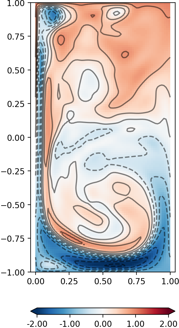
Based on a set of $p$ ensemble members, the ability of the proposed method to predict a trajectory associated with a new initial condition is demonstrated on a quasi-geostrophic barotropic model of a double-gyre [69] in a “rectangular-box ocean”. This idealistic model of North-Atlantic large-scale circulation considers the transport of the ageostrophic state variable components by a velocity in geostrophic balance. The adimensioned barotropic vorticity equation written for the potential vorticity $q$ and the stream function $\psi$ in $\Omega_{x}=\left([0:L]\times[-L:L]\right)$, with $L=1$, is

$$\left\{\begin{aligned} &\frac{\partial q}{\partial t}+J(\psi,q)=f-\left(\delta/L\right)^{5}\nabla^{4}\omega\\ &\Delta\psi=\omega\quad;\quad q=R_{o}\omega+y_{c},\end{aligned}\right.$$ (48)

where $\omega$ is the vorticity and $\boldsymbol{x}_{c}=(x_{c},y_{c})$ are the latitude and the longitude increasing eastward and northward, respectively, while $J(f,g)=\partial_{x}f\partial_{y}g-\partial_{x}g\partial_{y}f$ stands for the Jacobian (with $x$ and $y$ denoting horizontal and vertical coordinates of $\mathbb{R}^{2}$. In the model (48), the state of the system can be uniquely determined from the potential vorticity $q$. The set of all possible states of the system is then $\Omega\subset L^{2}(\Omega_{x},\mathbb{R})$ (i.e. $d=1$). The dimensionless Rossby number $R_{o}=0.0036$ measures the ratio between inertial forces and the Coriolis force, and a steady wind-forcing is defined as $f=\sin(\pi y_{c})$. The parameter $\delta/L=0.032$ controls the hyper-viscosity model, with $\delta$ the Munk boundary layer width. Scales smaller than $\delta$ will not be resolved. Numerical details and links with dimensional variables associated with a mid-latitude ocean basins, such as North Atlantic, as well as the way the initial conditions of the ensemble have been generated are given in E. Let us note that this system is ergodic when associated to an uncorrelated random forcing [70, 71, 72]. Here the forcing is stationary, and the system is not ergodic. As a consequence, such a system cannot be used for all the techniques relying on an ergodic assumption to extract a spectral representation of the Koopman operator.

5.2 Reconstructions using RKHS

In this study we focus only on two specific kernels: the empirical covariance kernel ($k_{E}$), and the Gaussian Kernel ($k_{G}$). They are defined respectively by

$$k_{E}(X_{t}^{(i)},\,X_{t}^{(j)})=\left\langle{{q}}^{(i)}(\bm{\cdot},t_{0})\,,\,{{q}}^{(j)}(\bm{\cdot},t_{0})\right\rangle_{\Omega_{x}},$$

and

$$k_{G}(X_{t}^{(i)},\,X_{t}^{(j)})=\exp{\frac{1}{{\ell_{G}}^{2}}\left\|{q}^{(i)}(\bm{\cdot},t_{0})-{q}^{(j)}(\bm{\cdot},t_{0})\right\|^{2}_{\Omega_{x}}},$$

where $\left\langle\bm{\cdot},\bm{\cdot}\right\rangle_{\Omega_{x}}$ stands for the standard $L^{2}$ inner product in $\Omega_{x}$ and $q^{(i)}(x,t)$ is the solution of equation (48) of the $i^{\text{th}}$ ensemble member at time $t$ at the space location $x$. The former has the advantage to be simple, and to be directly related to standard ensemble methods employed in data assimilation. However, it is strongly rank deficient and introduces spurious correlations in the physical domain $\Omega_{x}$ between two far apart locations. Localization techniques [73] have been introduced to tackle this problem and may be interpreted in our setting as embeddings in specific RKHS. This interpretation may open new computationally efficient generalisations related for instance to localization techniques in the model space as explained after remark 9. The parallel done between operators ${\cal L}^{\scriptscriptstyle{1/2}}_{k_{t}}$ and localization procedure should in particular enable to define time-varying and flow dependant localization techniques that are notably difficult to built in practice. Gaussian kernels are widely used in machine learning for its high regularity and non-compact support in $L^{2}(\Omega,\nu)$ [74]. It can be also interpreted as a way to perform localization. In this study, compared to other tested – but not presented – kernels (polynomial and exponential for instance), it led to better performances.

Once the kernel matrix $K_{ij}=k_{t}(X_{t}^{(i)}\,,\,X_{t}^{(j)})$ for $(i,j)\in[1\dots p]\times[1\dots p]$ (equal for all $t$ – kernels isometry, Theorem 3) is evaluated, a very simple reconstruction of the whole trajectory can be performed. Denoting $X^{\prime}_{0}$ a new ensemble member initial condition, the linear combination vector $\bm{\beta}$ associated to the reconstructed trajectory $\hat{X}^{\prime}_{t}=\sum_{i=1}^{p}\beta_{i}X_{t}^{(i)}$ can be estimated by kernel regression from the evaluation $k(X^{\prime}_{0},X_{0}^{j})$, for $j=[1\dots p]$, and the reproducing property as

$$\bm{\beta}=K^{-1}k(X^{\prime}_{0}\,,\,X_{0}^{[1\dots p]}).$$ (49)

Strikingly, Koopman isometry implies that these coefficients are constant along time, and brings hence a direct reconstruction of the whole trajectory.

5.3 Evaluation of the Koopman eigenfunctions

Performing the $\mathcal{H}_{t}$ inner product of equation (7) with the ensemble members’ feature maps leads to the matrix

$$\mathbb{M}(X_{t}^{(i)},\,X_{t}^{(j)})=\left(-{\partial_{{\cal M}(\bm{\cdot})}}\,k_{t}(\bm{\cdot},X_{t}^{(j)})\right)\left(X_{t}^{(i)}\right).$$ (50)

As explained previously eigen-elements of $\mathbb{M}K^{-1}$, noted $(\lambda_{\ell},V_{\ell}(X_{t}^{(i)}))$, give access to the exact evaluation of Koopman eigenfunctions on the RKHS family at the ensemble members $\psi_{\ell}^{t}(X_{t}^{(i)})={\cal L}_{k}^{\scriptscriptstyle{1/2}}V_{\ell}(X_{t}^{(i)})$, and to the associated eigenvalues $\lambda_{\ell}$. We note that $\partial_{{\cal M}(\bm{\cdot})}k_{t}(\bm{\cdot}\,,\,X_{t}^{(j)})$ is obtained by differentiating the kernel expression (see equations 46, 47 for the two selected kernels). Skew-symmetry of $\mathbb{M}K^{-1}$, inherited from the skew-symmetry of $A_{U\!,\,t}$, is only approached numerically. Evaluations are thus enhanced by considering only the skew-symmetric part of the matrix $\mathbb{M}K^{-1}$, which is dominant in the numerical evaluation of (50).

5.4 Lyapunov times

The Lyapunov times evaluated using the two kernels $k_{E}$ and $k_{G}$ are compared. Three methods to compute the Lyapunov exponents $\sigma$ are detailed in section 4.3. The associated Lyapunov times are defined by $T=\sigma^{-1}\ln C$, with, $C=10^{3}$.

The Lyapunov times associated with exponents expressed in $L^{2}_{\mathbb{C}}(\Omega_{t},\nu)$ are shown in figure 1(a). The spectrum associated with all singular values, truncated such that $\sigma>10^{-5}$, is displayed. Due to this truncation, very slow modes are not well captured. We can see that the Gaussian kernel $k_{G}$ estimates in average larger Lyapunov times.

Refer to caption
(a) Lyapunov times spectrum expressed in $L^{2}_{\mathbb{C}}(\Omega_{t},\nu)$ for the Gaussian kernel $k_{G}$ and the empirical covariance $k_{E}$.
Refer to caption
(b) Modal Lyapunov times associated with individual Koopman modes. Comparison with expression in $L^{2}_{\mathbb{C}}(\Omega_{t},\nu)$ and in $\mathcal{H}_{t}$.
Figure 1: Lyapunov times computed using the Gaussian kernel $k_{G}$ and the empirical covariance kernel $k_{E}$.

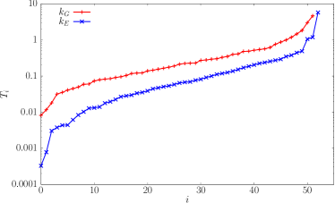
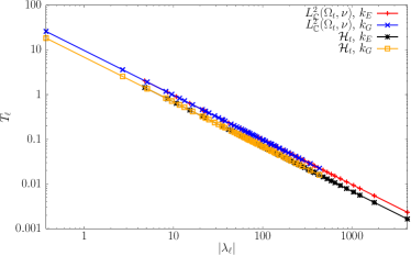
In figure 1(b), the Koopman modal Lyapunov times are shown as a function of the absolute value of the Koopman eigenvalue. The Lyapunov times expressed with the RKHS norm equation (45) is directly $T_{\ell}=1/|\lambda_{\ell}|\ln C$, which explains the perfect decaying slope in logarithmic scale. We observe that the computation of the modal exponents in $L^{2}_{\mathbb{C}}(\Omega_{t},\nu)$ leads simply to a vertical shift of the curves due to the scaling factor induced by the change of norm. We can notice that with the Gaussian kernel $k_{G}$, slower Koopman eigenfunctions are evaluated compared to $k_{E}$, which leads to longer Lyapunov times. This explains longer predictions, which will be presented in section 5.5. As it will be seen, the modal exponents and their associated Lyapunov times will reveal very useful, as they will allow us to filter out sequentially the contributions of the Koopman eigenfunctions beyond their predictability time.

5.5 Reconstructions

The ability of trajectories reconstruction is illustrated in figure 2, where a full trajectory is estimated from the embedding of a new initial condition in the RKHS family. We compare the anomaly (figure 2(a)) of a given new ensemble member at an advanced time (3.7 days), with reconstructions using the Gaussian kernel $k_{G}$ (figure 2(c)). Figure 2(b) shows the best possible reconstruction as a linear combination of ensemble members, with regards to the $L^{2}(\Omega_{x})$-norm of the projection error.

Refer to caption
(a) Test ensemble member
Refer to caption
(b) $L^{2}$norm projection
Refer to caption
(c) Gaussian kernel
Figure 2: Comparison between the reference potential vorticity of a test ensemble member at $t=0.07$ (corresponding to $3.7$ days of prediction) (a) and the predicted reconstruction using the Gaussian kernel (${\ell_{G}}=1$) (c). The best possible reconstruction using a linear combination of ensemble members with respect to the $L^{2}$ norm is shown in (b).

Reconstruction errors are quantified by averaging the square of the $L^{2}(\Omega_{x})$-norm over the whole test ensemble composed of $100$ new members (i.e. not used in the training phase). The standard deviations of the error are also displayed on this figure. The time evolution of this error is presented in figure 3. It is compared to the projection error defined as the minimal linear combinations of ensemble members with a constant-in-time coefficient w.r.t. $L^{2}(\Omega_{x})$-norm. The reconstruction error performed by the ensemble average is also shown. This error is obviously high for small times, but estimations are difficult to be more precise than the ensemble average estimation once the predictability time of the system has passed. The reconstructions performed with $k_{E}$, grow and overtake the ensemble average reconstruction around $t=0.2$ (i.e. $18.4$ days). On this basis, the use of $k_{G}$ (${\ell_{G}}=1.0$) leads to better results. Indeed, despite a slight reconstruction penalty at the initial time due to a stronger smoothing (see figure 2), the reconstruction errors become quickly significantly lower, and the error never reaches the ensemble anomaly error. This small loss of performance in $L^{2}(\Omega_{x})$-norm at the initial time allows to have a gain in robustness in terms of long-time prediction. Let us note that the lengthscale parameter $\ell_{G}$ is sensitive. In this work, we fixed it a priori. However, techniques that aim at learning such a parameter have been proposed in [5, 6].

Refer to caption
Figure 3: Mean estimation error using an empirical covariance kernel (short red dashes), a Gaussian kernel (green dash-dots), the reconstructed Gaussian kernel using all Koopman eigenfunctions (orange squares) and the Lyapunov filtered kernel (blue dot-dashes). “Ensemble average” (long black dashes) is the estimation error of the ensemble average. The projection error (purple solid line) corresponds to the optimal constant-in-time linear combination of ensemble members w.r.t. the $L^{2}(\Omega_{x})$-norm. The vertical width of the stripes regions over the mean error is equal to the standard deviation of the error. One dimensionless time $t$ corresponds to $92$ days. Errors are averaged over the $100$ members of the test ensemble.

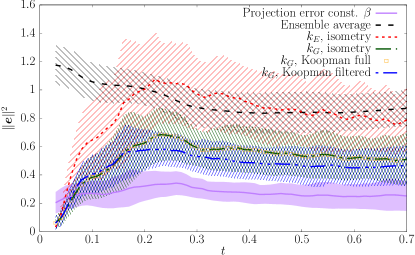
The reconstructions based on (49) are valid for all times. Koopman isometry warrants the use of the same linear combination for the whole trajectory. Nevertheless, in practice the ensemble are of limited (small) size, and the eigenpairs of the infinitesimal generator close to zero (representing almost stationary functions) are difficult to estimate accurately. Modal predictability time associated to Lyapunov exponents (44) can be used to robustify the forecast of new initial conditions. The kernel can be expanded in the Koopman eigenfunctions basis as

$$k(X_{t}^{(i)},\,X_{t}^{(j)})=\sum_{{\color[rgb]{0,0,0}\ell}=1}^{\infty}\psi_{\ell}^{t}(X_{t}^{(i)})\overline{\psi_{\ell}^{t}}(X_{t}^{(j)})=\sum_{{\color[rgb]{0,0,0}\ell}=1}^{\infty}\psi_{\ell}^{0}(X_{0}^{(i)})\overline{\psi_{\ell}^{0}}(X_{0}^{(j)}).$$ (51)

With the numerical procedure proposed here, the $p$ evaluated Koopman eigenfunctions allow to perform an exact reconstruction of the kernel. An appealing potential of equation (51) for faithful predictions consists in filtering the kernel by switching-off components that have passed their predictability time. We set this time from the finite-time Lyapunov exponents (44) as: $T_{\ell}=|\lambda_{\ell}|^{-1}\ln C$, with, $C=10^{3}$. The filtered kernel $\widetilde{k}(X_{t}^{(i)},\,X_{t}^{(j)})$ and its associated $p\times p$ kernel matrix $\widetilde{K}$ allows us to define reconstructions, with the modified linear coefficients $\widetilde{\bm{\beta}}=\widetilde{K}^{+}\widetilde{K}\bm{\beta}$. The superscript $\bullet^{+}$ stands for the Moore–Penrose pseudo-inverse. It can be remarked that the operator $\widetilde{K}^{+}\widetilde{K}$ is a projector performing filtering directly on the vector of coefficients $\bm{\beta}$.

In figure 3, it is assessed that the kernel is exactly reconstructed by the Koopman eigenfunctions (superimposition of the green dash-dots curve and the orange squares). When the kernel is Lyapunov filtered, the reconstruction almost fits at short time the previous predictions (superimposition of the blue dot-dashes curve, the green dash-dots curve and the orange squares). For longer time it significantly reduces the error and clearly separates the spread of the ensemble from the ensemble average estimation. For very long times (not shown in the figure), filtering acts on all modes, which reduces to the ensemble average estimation. This strategy takes advantage of the modal predictability time. Slow eigenfunctions are used for long time predictions, and fast ones only for short time forecasts. As a final remark, we note that very fast modes (with large Koopman eigenvalues modulus) does not seem to contribute significantly to the reconstruction, since at short times the filtered and full reconstructions match.

5.6 Data assimilation

A possible application of the proposed procedure is ensemble-based data assimilation. In the context of satellite data, ensemble optimal interpolation (EnOI) is widely used to reconstruct spatial fields [75, 76]. It is for instance employed in operational gridded altimetry reconstructions [77]. EnOI consists in expressing at a given time the solution as a linear combination of ensemble members, which minimises an objective cost function. As shown in [78, 79], incorporating information from other times together with an adequate dynamical model significantly improves the estimations. This is obviously at the price of forecasting the whole ensemble by the dynamics.

Koopman isometry provided by the RKHS family allows us to incorporate time-series of observations without any new simulation of the dynamics. The spatial reconstruction is embarrassingly simply given as the constant-in-time best linear combination of ensemble members trajectories.

Based on the same ensemble as in the previous sections, we propose two demonstration tests considering i) a time-series of extremely sparse (two satellite swaths like) observations ii) an even sparser case with the same swaths but at a single time only. To that end, we consider a synthetic observation mimicking two along tracks measurements of an orbiting satellite, idealized by two vertical lines. In the first case these lines are assumed to be known every $0.9$ days $\Delta t=0.01$, while in the second case only day $5.5$ is available $(t=0.06)$. The observations are perturbed by a centered Gaussian white noise with the value of the selected standard deviation equal to 10% of the signal root-mean-square. These 2 benchmarks are carried out for each of the 100 members of the test ensemble. As previously, the members of the test ensemble have not been used in the learning phase.

In this numerical experiment, we search for the constant in time coefficients $\bm{\beta}$ (thanks to isometry), which minimises

$$\mathcal{J}=\frac{1}{2T}\int_{0}^{T}\|\mathbb{H}(\hat{X}_{t})-\mathcal{Y}\|_{R^{-1}}^{2}\,\mathrm{d}t+\frac{\alpha^{2}}{2}\|\bm{\beta}{-\bar{\bm{\beta}}}\|^{2}\text{ s.t. }\mathbb{H}(\hat{X}_{t})=\sum_{i=1}^{p}\beta_{i}\mathbb{H}(X_{t}^{(i)}),$$ (52)

where $\mathbb{H}$ is the observation operator associated with the satellite measurements $\mathcal{Y}$, $\hat{X}_{t}$ is the estimated state, and $\bar{\beta}=\frac{1}{p}(1,\dots,1)^{T}$. The observation operator is assumed to have its range in the RKHS family and hence provides observables belonging to the RKHS family, which can be interpolated using the RKHS family kernels. It can be noticed that the expression of the constraint is due to kernel interpolation, and not to some linear property of $\mathbb{H}$. This treatment is similar to the one performed for instance in discrete empirical interpolation (DEIM) [80]. In the case of a single observation, the time integral is dropped, and the cost function corresponds to a standard EnOI cost function. The matrix $R$ is the observation covariance matrix, defined by the time average of the empirical covariance, localized by performing a Schur product with matrix $\exp{(-r_{ij}^{2}/\ell_{loc}^{2})}$, where $r_{ij}$ is the distance between measurements $i$ and $j$, and $\ell_{loc}=0.05$. The regularization parameter has been set to $\alpha=10$. For this problem we selected the simple empirical kernel, defined from a non localized potential vorticity matrix as feature maps of the ensemble. Working with the isometry property justifies the estimation of constant in time coefficients for the linear combination. This simplistic method could be easily extended by introducing more elaborated kernels, Koopman eigenfunctions representation to project any system’s observable and forecast them, as well as the Lyapunov filtering schme presented in section (5.5).

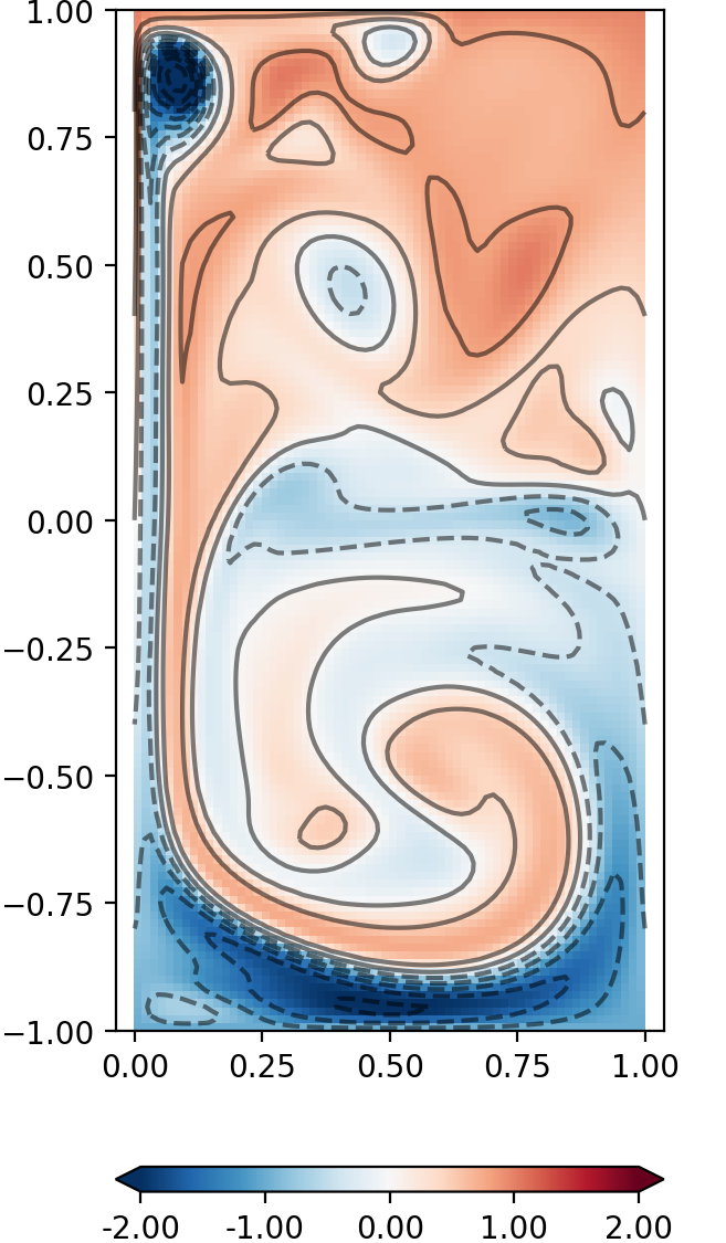
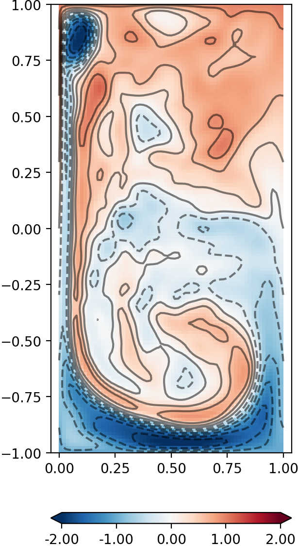
Figure 4 shows the potential vorticity trajectory (panel a), the single-time observation (panel b), the trajectory reconstruction associated to this single observation (panel c) and the one obtained from the swaths time-series (panel d). Three consecutive times spaced of $0.02$ (1.8 days) are displayed.

Refer to caption
Figure 4: Estimation of potential vorticity at times $t=0.04$ (top), $t=0.06$ (middle) and $t=0.08$ (bottom). Panel (a): True anomaly. Panel (b): Observation associated with the single-time swath observation. Panel (c): Estimation knowing the two satellite swaths only at day 5.5 $(t=0.06)$. Panel (d): Estimation knowing the two swaths every 0.9 days $(\Delta t=0.01)$.

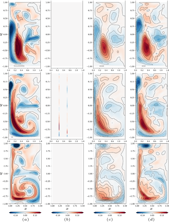
We can see that despite extremely sparse measurements, a single observation already provides a fairly good estimation, together with forward and backward in time forecasts based only on the estimated linear combination of the ensemble members (i.e. without any simulation). As expected, a time-series of swaths improves further the performances.

In figure 5, the average of the errors obtained over all $100$ members of the test ensemble are plotted.

Refer to caption
Figure 5: Estimation errors averaged over the whole $100$ members of the test ensemble. The best reconstruction error with constant coefficients (purple), estimation by the ensemble average (black), estimation with the time-series of satellite swaths observations (yellow) and only at day $5.5$ $(t=0.06)$ (blue).

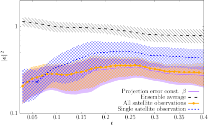
As a reference, the best possible reconstruction with respect to the $L^{2}$ norm with constant in time linear coefficients $\bm{\beta}$ is shown, as well as the estimation by the ensemble average. The error performed with the time-series of satellite observations is almost optimal in terms of average and standard deviation. We note that for the second test-case, near the observation time, the error is lower than the one obtained for the whole time-series. Compared to the time series of observations it may be interpreted as an over-fitting at the observation time since only a single observation is used to infer the ensemble members’ coefficients. As expected, this error grows, but reasonably, as the estimation is propagated forward and backward in time. As a final remark, let us emphasize that considering time series of the sparse observables (in space and time) such as the satellite swaths considered in this study, which constitute typical altimetric observations of the ocean surface, would require an extremely long series to reconstruct the Koopman eigenpairs (see [34]) at the scale of a large basin such as the North Atlantic basin. For geophysical flows this can be highly problematic in the nowadays state of the fast climate change we are observing. The proposed technique, based on an ensemble of realizations instead of time series, constitutes a promising alternative to face these difficulties. We assessed here the technique with an idealistic dynamics model and more realistic models need to be tested. This will be the subject of future works.

6 Concluding remarks

We proposed a theoretical setting to estimate the Koopman eigen-pairs of compact dynamical systems in embedding the system in a RKHS family. Beyond the Koopman operator spectral representation, we showed that the RKHS family provides access to finite time Lyapunov exponents, as well as to the tangent linear dynamics. These features enabled us to propose very simple strategies for data assimilation of very sparse observations in time and space. Obviously more efficient data assimilation techniques could be used instead of the simple regression strategy explored here. As the RKHS family boils down to a linear setting it should be perfectly adapted to ensemble Kalman filters. Extension of classical ensemble data assimilation filters on the RKHS family are currently in development and will be the subject of future publications. The technique lies on the sequence of time-evolving RKHS to represent the ensemble dynamics and on the superposition principle attached to the RKHS family. This study provides a theorem-based setting to estimate the Koopman eigenvalues and eigenfunctions, as well as exact ensemble-based representation of the tangent linear dynamics and of the flow Lyapunov exponents. This work relies on the assumption of an invertible deterministic dynamical system defined on a compact manifold. In future studies, we will focus on the generalisation to stochastic fluid flow dynamics with transport noise models [81, 82, 83, 84] and the introduction of more sophisticated ensemble data assimilation techniques [85, 86].

Acknowledgments

The authors acknowledge the support of the ERC project 856408-STUOD and the French National program LEFE (Les Enveloppes Fluides et l’Environnement).

Appendix A Reproducing kernel Hilbert spaces

In the following appendices we provide complementary elements for the detailed proofs of the results listed in the paper. We first recall some classical theorems on RKHS and present their adaptations to our functional setting. In particular we present useful results on differentiability of RKHS functions and reproducing kernels. In the following $L^{2}(\Omega_{x})$ stands for the Hilbert space of Lebesgue measurable $\mathbb{R}^{d}$-valued of square-integrable functions on the set $\Omega_{x}\subset\mathbb{R}^{p}$ $p=2,3$ endowed at a fixed time, $t$, with the inner product

$$\langle f\,,g\rangle_{L^{2}(\Omega_{x})}=\int_{\Omega_{x}}f(y)\,\,g(y)\;\mathrm{d}y.$$

Let $E\subset L^{2}(\Omega_{x})$ denote a compact subset equipped with the norm of $L^{2}(\Omega_{x})$, by the Aronszajn Theorem, [59], the reproducing kernel Hilbert spaces (RKHS) of $\mathbb{C}$-valued functions defined on $E$ are uniquely characterized through a reproducing kernel $k:E\times E\mapsto\mathbb{C}$. This kernel is a Hermitian, positive definite function. In the following we will assume furthermore it is $C^{{(}1,1{)}}(E\times E)$, which means here it is twice differentiable with respect to its two variables. The (Gateaux) derivative with respect to the first and second variable in the direction $v\in E$ are denoted $\partial_{v}^{\tiny{(1)}}k$, and $\partial_{v}^{\tiny{(2)}}k$, respectively. The reproducing kernel defines an evaluation function $k(\bm{\cdot},x)\in{\cal H}$ with a reproducing property (Def. 1):

$$\forall x\in E,\forall f\in{\cal H},\;\bigl{\langle}f,k(\,\bm{\cdot}\,,\,x)\bigr{\rangle}_{{\cal H}}=f(x).$$

The RKHS ${\cal H}$ corresponds to a space of functions with a strong uniform convergence property. The elements of ${\cal H}$ are in addition continuous functions and we have for all $f\in{\cal H}$ that

$$\forall\,x\in E\qquad\left|f(x)\right|\,\leq\,\sup_{y\in E}k(y,y)^{1/2}\;\|f\|_{{}_{\cal H}}.$$ (53)

A.1 Functional description of ${\cal H}$

We recall in the following the Mercer’s theorem which gives a functional description of the RKHS ${\cal H}$ and of its associated reproducing kernel $k$.
Let $L^{2}_{\mathbb{C}}(E,\nu)$ be the space of measurable complex valued functions defined on the compact set E for which the square modulus is integrable with respect to measure $\nu$, $L^{2}_{\mathbb{C}}(E,\nu)$ is a Hilbert space equipped with the inner product $\langle\bm{\cdot}\,,\,\bm{\cdot}\rangle_{{L^{2}_{\mathbb{C}}(E,\nu)}}$ given for $f$ and $g\in L^{2}_{\mathbb{C}}(E,\nu)$ by

$$\langle f\,,\,g\rangle_{{L^{2}_{\mathbb{C}}(E,\nu)}}:=\int_{E}f(y)\,\overline{\,g(y)\,}\;\nu(\mathrm{d}y),$$

so that it is linear in its first argument and antilinear in its second. Let us first define ${\cal L}_{k}:L_{\mathbb{C}}^{2}(E,\nu)\mapsto L_{\mathbb{C}}^{2}(E,\nu)$ the integral operator with kernel ${k\in{C^{{(}1,1{)}}}(E\times E)}$ as:

$$\bigl{(}{\cal L}_{k}f\bigr{)}(x)=\int_{E}k(x,y)f(y)\,\nu(\mathrm{d}y).$$ (54)

We give below a useful remark relating the integral operator $\mathcal{L}_{k}$ and the inner product $\langle\bm{\cdot}\,,\,\bm{\cdot}\rangle_{L^{2}_{\mathbb{C}}(E,\nu)}$.

Remark 10 (Links between $\mathcal{L}_{k}$ and $\langle\,\bm{\cdot}\,,\,\bm{\cdot}\,\rangle_{L^{2}_{\mathbb{C}}(E,\nu)}$)

As $k$ is Hermitian, it can be noticed that for all $x\in E$, $\bigl{(}{\cal L}_{k}f\bigr{)}(x)=\int_{E}f(y)\,\overline{k(y,x)}\,\nu(\mathrm{d}y)$, and we have thus $\bigl{(}{\cal L}_{k}f\bigr{)}(x)=\langle f\,,\,k(\,\bm{\cdot}\,,\,x)\rangle_{L^{2}_{\mathbb{C}}(E,\nu)}$.

This kernel integral operator can be shown to be well-defined and compact (by Arzelà Ascoli theorem). It is immediate to see that as $k$ is positive definite and Hermitian, ${\cal L}_{k}$ is positive and self-adjoint on $L_{\mathbb{C}}^{2}(E,\nu)$. By the spectral theorem of compact self-adjoint operators, there exists an orthonormal basis $(\varphi_{i})_{i}$ of $L_{\mathbb{C}}^{2}(E,\nu)$ consisting of eigenvectors of ${\cal L}_{k}$ with corresponding decreasing real eigenvalues $(\mu_{i})_{i}$ : $\mu_{i}\geq\mu_{i+1}\geq 0$ for all integers $i$. These results are proved in [58]. We consider in the following that $\mu_{i}\neq 0$ for all $i$ and $\mathcal{L}_{k}$ is injective. This denseness assumption could be relaxed (see remark 16) but simplifies significantly the presentation. The eigenpairs $(\mu_{i},\varphi_{i})_{i\in\mathbb{N}}$ enables to formulate the following theorems (with proofs available for instance in [58] and [60]). Elaborating on remark 10 and the kernel eigenfunctions (often referred to as Mercer’s eigenfunctions due to theorem 4) we get immediately relations between the eigenfunction evaluation and the $L^{2}(E,\nu)$ inner product.

Remark 11 (Links between $(\varphi_{i})_{i\geq 0}$ and $\langle\bm{\cdot}\,,\,\bm{\cdot}\rangle_{L^{2}_{\mathbb{C}}(E,\nu)}$)

For all $x\in E$, by Remark 10, we note that

$\displaystyle\langle\varphi_{i}\,,\,k(\,\bm{\cdot}\,,\,x)\rangle_{L^{2}_{\mathbb{C}}(E,\nu)}\;=\;\mathcal{L}_{k}(\varphi_{i})(x)\;=\;\mu_{i}\,\varphi_{i}(x)\qquad\text{and}$
$\displaystyle\langle k(\,\bm{\cdot}\,,\,x)\,,\,\varphi_{i}\rangle_{L^{2}_{\mathbb{C}}(E,\nu)}\;=\;\overline{\langle\varphi_{i}\,,\,k(\,\bm{\cdot}\,,\,x)\rangle}_{L^{2}_{\mathbb{C}}(E,\nu)}\;=\;\mu_{i}\,\overline{\varphi_{i}(x)}.$

Remark 12

As $k\in{C^{{(}1,1{)}}}(E\times E)$, the range of $\mathcal{L}_{k}$ is included in $C^{1}(E)$ and the eigenfunctions of $\mathcal{L}_{k}$ are $C^{1}(E)$.

Theorem 4 (Mercer decomposition)

For all $x$ and $y\in E$, $\displaystyle k(x,y)=\sum_{i=0}^{\infty}\mu_{i}\,\varphi_{i}(x)\;\overline{\varphi_{i}(y)}$ where the convergence is absolute (for each $x,y\in E\times E$) and uniform on $E\times E$.

In particular, the series $\sum\mu_{i}$ is convergent as

$$\displaystyle\int_{E}k(y,y)\nu({\mathrm{d}}y)=\int_{E}\sum_{i=0}^{\infty}\mu_{i}\varphi_{i}(y)\;\overline{\varphi_{i}(y)}\nu({\mathrm{d}}y)=\sum_{i=0}^{\infty}\mu_{i}<\infty.$$ (55)
Theorem 5 (Mercer representation of RKHS)

The RKHS $\left({\cal H},\langle\,\bm{\cdot}\,,\,\bm{\cdot}\,\rangle_{{}_{\cal H}},\|\bm{\cdot}\|_{{\cal H}}\right)$ is the Hilbert space characterized by

$$\displaystyle{\cal H}=\bigl{\{}f\in L_{\mathbb{C}}^{2}(E,\nu),\;f=\sum_{i=0}^{\infty}a_{i}\varphi_{i}\;:\;\sum_{i}\dfrac{\,|a_{i}|^{2}}{\mu_{i}}<\infty\bigr{\}},$$
$$\bigl{\langle}f,g\bigr{\rangle}_{{\cal H}}=\sum_{i=0}^{\infty}\frac{1}{\mu_{i}}\,\langle f\,,\,\varphi_{i}\rangle_{L^{2}_{\mathbb{C}}(E,\nu)}\,\overline{\langle g\,,\,\varphi_{i}\rangle}_{L^{2}_{\mathbb{C}}(E,\nu)}\quad$$
$$\text{and}\quad\|f\|^{2}_{{}_{\cal H}}=\sum_{i=0}^{\infty}\frac{|\langle f\,,\,\varphi_{i}\rangle_{L^{2}_{\mathbb{C}}(E,\nu)}|^{2}}{\mu_{i}}.$$

The inner product $\langle\,\bm{\cdot}\,,\,\bm{\cdot}\,\rangle_{{}_{\cal H}}$ is sesqui-linear (linear in its first argument and antilinear in its second). The proof of Mercer’s theorem warrants that the linear space spanned by $\{k(\,\bm{\cdot}\,,x):x\in E\}$ is dense in $L^{2}_{\mathbb{C}}(E,\nu)$. If $f=\sum_{i=0}^{\infty}a_{i}\varphi_{i}\in{\cal H}$ then the series converges absolutely and uniformly to $f$.

The following remark shows that the feature map’s conjugate as well as its real and imaginary parts belong to ${\cal H}$.

Remark 13 (Consequence of the Mercer representation)

For all $y\in E$, the functions $\overline{\,k(\,\bm{\cdot}\,,\,y)}$,   $Re[k(\,\bm{\cdot}\,,\,y)]$ and $Im[k(\,\bm{\cdot}\,,\,y)]$ belong to ${\cal H}$. By Theorems 5 and 4, we have indeed that

$$\sum_{i=0}^{\infty}\dfrac{1}{\mu_{i}}\,|\langle\overline{\,k(\,\bm{\cdot}\,,\,y)\,}\,,\,\varphi_{i}\rangle_{L^{2}_{\mathbb{C}}(E,\nu)}|^{2}\;=\;\\ \sum_{i=0}^{\infty}\dfrac{1}{\mu_{i}}\,|\,\mathcal{L}_{k}\varphi_{i}(y)|^{2}=\sum_{i=0}^{\infty}\mu_{i}\,|\varphi_{i}(y)|^{2}<\infty,$$ (56)

and $\overline{\,k(\,\bm{\cdot}\,,\,y)}\in{\cal H}$. By operation, $Re[k(\,\bm{\cdot}\,,\,y)]$ and $Im[k(\,\bm{\cdot}\,,\,y)]$ belong thus to ${\cal H}$.

Remark 14 (Comparison of the norms ${\cal H}$ and $L_{\mathbb{C}}^{2}(E,\nu)$)

For all $f\in{\cal H}$, by Theorem 5 we have for all $x\in E$, the inequality

$$\displaystyle f(x)\leq|f(x)|=\left|\sum_{i=0}^{\infty}a_{i}\varphi_{i}(x)\right|\leq\left(\sum_{i=0}^{\infty}\dfrac{\,|a_{i}|^{2}\,}{\mu_{i}}\right)^{\scriptscriptstyle{1/2}}\;\left(\sum_{i=0}^{\infty}\mu_{i}|\varphi_{i}(x)|^{2}\right)^{\scriptscriptstyle{1/2}},$$

with theorem 4 we obtain

$$\displaystyle\|f\|_{{L_{\mathbb{C}}^{2}(E,\nu)}}\;\leq\;\left(\int_{E}|k(x,x)|^{2}\,\nu(\mathrm{d}x)\right)^{\scriptscriptstyle{1/2}}\,\|f\|_{{}_{\cal H}}.$$ (57)

Remark 15

For all $f\in L^{2}_{\mathbb{C}}(E,\nu)$ , $\mathcal{L}_{k}(f)$ belongs to ${\cal H}$, in fact we have

$$\sum_{i=0}^{\infty}\frac{1}{\mu_{i}}\left|\langle\mathcal{L}_{k}(f)\,,\,\varphi_{i}\rangle_{L^{2}_{\mathbb{C}}(E,\nu)}\right|^{2}=\sum_{i=0}^{\infty}\mu_{i}\left|\langle f\,,\,\varphi_{i}\rangle_{L^{2}_{\mathbb{C}}(E,\nu)}\right|^{2}\leq\left(\sum_{i=0}^{\infty}\mu_{i}\,\right)\,\|f\|^{2}_{L^{2}_{\mathbb{C}}(E,\nu)}<\infty.$$

Moreover, by Remark 14 the mapping $\mathcal{L}_{k}:{\cal H}\to{\cal H}$ is continuous : for all $f\in{\cal H}$ we have

$$\|\mathcal{L}_{k}(f)\|^{2}_{{\cal H}}\leq\left(\sum_{i=0}^{\infty}\mu_{i}\,\right)\;\|f\|^{2}_{L^{2}_{\mathbb{C}}(E,\nu)}\leq C\,\|f\|^{2}_{{\cal H}}.$$

With a $C^{{\color[rgb]{0,0,0}(1,1)}}(E\times E)$ regularity condition on the kernel, we will prove that the RKHS ${\cal H}$ is a subspace of smoother functions than $C^{0}(E,\mathbb{C})$ (theorem 6). In the following appendix we discuss differentiability property of the feature maps.

A.2 Differentiability of feature maps and RKHS functions ${\cal H}$

In this appendix we extend results given in [87, 88, 56] for $E\subset\mathbb{R}^{d}$ to the case where $E$ is a compact subset of a function vector space. In the following, aligned with the assumptions enunciated in the paper’s preamble, $E$ designates a compact set included in $L^{2}(\Omega_{x},\mathbb{R}^{d})$, the space of measurable functions that are square integrable on $\Omega_{x}$, and like [56], to enable differentiability of the RKHS function, we will assume that $E$ is the closure of its nonempty interior $\overset{\circ}{E}$. We assume also that $\nu$ is a finite measure on $E$, (i.e. $\nu(E)<\infty$). Denoting by $\partial^{(2)}_{u}\,k(\,\bm{\cdot}\,,y)$ the kernel functional derivative in the direction $u$ with respect to the second variable $y$ – while the upper-script ${\partial_{u}^{(1)}}$ indicates a directional derivative in the first variable –, we have first the following lemma on the feature maps derivative.

Lemma 2 (Feature maps differentiability)

The kernel derivatives belong to ${\cal H}$. More precisely, let $k\in{C^{(1,1)}}(E\times E)$, then for all $y\in E$ and ${u}\in E$, we have $\partial^{(2)}_{{u}}\,k(\,\bm{\cdot}\,,y)\in{\cal H}$.

Proof

Let $y\in{\color[rgb]{0,0,0}\overset{\circ}{E}}$ and ${u}\in E$. Let $(h_{n})_{n\geq 0}$ be a sequence of $\mathbb{C}\backslash\{{0}\}$ which converges to 00 and such that for all $n$, $y+h_{n}{u}\in{\color[rgb]{0,0,0}\overset{\circ}{E}}$ (since ${\color[rgb]{0,0,0}\overset{\circ}{E}}$ is an open set). For all integers $n$, let

$$d_{n}(\,\bm{\cdot}\,,\,y):=k(\,\bm{\cdot}\,,\,y+h_{n}{u})-k(\,\bm{\cdot}\,,\,y)\text{ and }\;t_{n}(\,\bm{\cdot}\,,\,y\,):=\dfrac{\,d_{n}(\,\bm{\cdot}\,,\,y)\,}{h_{n}}.$$

We first notice that $(t_{n}(\bm{\cdot}\,,\,y))_{n\geq 0}$ converges pointwise to ${\partial^{(2)}_{{u}}}\,k(\,\bm{\cdot}\,,\,y)$ since $k$ is ${C^{(1,1)}}(E\times E)$. Then, we now show that $(t_{n}(\,\bm{\cdot}\,,\,y))_{n}$ is a Cauchy sequence of $({\cal H},\|\bm{\cdot}\|_{{}_{\cal H}})$. For all integers $p$ and $q$, we have

$$\|t_{p}(\,\bm{\cdot}\,,\,y)-t_{q}(\,\bm{\cdot}\,,\,y)\|^{2}_{{}_{\cal H}}=\|t_{p}(\,\bm{\cdot}\,,\,y)\|^{2}_{{}_{\cal H}}+\,\|t_{q}(\,\bm{\cdot}\,,\,y)\|^{2}_{{}_{\cal H}}-2Re[\langle\,t_{p}(\,\bm{\cdot}\,,\,y)\;,\;t_{q}(\,\bm{\cdot}\,,\,y)\,\rangle_{{}_{\cal H}}].$$ (58)

By the reproducing property of ${\cal H}$ and as $k$ is ${C^{(1,1)}}(E\times E)$, we have for all $x\in E$ and for some $p$ and $q$ large enough,

$\displaystyle\langle\,t_{p}(\,\bm{\cdot}\,,\,y)\;,\;t_{q}(\,\bm{\cdot}\,,\,x)\,\rangle_{{}_{\cal H}}$ $\displaystyle=\dfrac{1}{h_{p}\,h_{q}}\langle\,k(\,\bm{\cdot}\,,\,y+h_{p}u)-k(\,\bm{\cdot}\,,\,y)\,\;,\;k(\,\bm{\cdot}\,,\,x+h_{q}u)-k(\,\bm{\cdot}\,,x)\,\rangle_{{}_{\cal H}}$
$\displaystyle=\dfrac{1}{h_{p}\,h_{q}}\,\left(\,k(x+h_{q}u\,,\,y+h_{p}u)-k(x\,,\,y+h_{p}u)-k(x+h_{q}u\,,\,y)+k(x,y)\,\right)$
$\displaystyle=\dfrac{1}{h_{p}\,h_{q}}\,\left(\,\partial^{(1)}_{u}k(x\,,\,y+h_{p}u)\,\times\,h_{q}-\partial^{(1)}_{u}k(x\,,\,y)\times h_{q}+o(h_{q})\,\right)$
$\displaystyle=\partial^{(2)}_{u}\,\partial^{(1)}_{u}k(x\,,\,y)+o_{p,q}(1)$

We have also for some $p$ and $q$ large enough (with $y=x$) and $\varepsilon>0$,

$$\left|\bigl{\langle}\,t_{p}(\,\bm{\cdot}\,,\,y)\;,\;t_{q}(\,\bm{\cdot}\,,\,y)\,\bigr{\rangle}_{{}_{\cal H}}-\partial^{(2)}_{{u}}\partial^{(1)}_{{u}}k(y\,,\,y)\right|\leq\varepsilon,$$

and by (58) we obtain hence $\|t_{p}(\,\bm{\cdot}\,,\,y)-t_{q}(\,\bm{\cdot}\,,\,y)\|^{2}_{{}_{\cal H}}\leq 4\varepsilon$, which means $\bigl{(}t_{n}(\,\bm{\cdot}\,,\,y)\bigr{)}_{\!n}$ is a Cauchy sequence in ${\cal H}$. The sequence $\bigl{(}t_{n}(\,\bm{\cdot}\,,\,y)\bigr{)}_{\!n}$ converges to a function $t(\,\bm{\cdot}\,,\,y)$ in ${\cal H}$ and by (53) the convergence is pointwise. Consequently, we obtain also $\partial^{(2)}_{{u}}\,k(\,\bm{\cdot}\,,\,y)=t(\,\bm{\cdot}\,,\,y)\in{\cal H}$ for $y\in\overset{\circ}{E}$.

Let $y\in E\backslash\overset{\circ}{E}$. There exists a sequence $(y^{i})$ of $\overset{\circ}{E}$ converging to $y$. For all integers $i$ and $j$, we have,

$$\|\partial^{(2)}_{{u}}\,k(\,\bm{\cdot}\,,\,y^{i})-\partial^{(2)}_{{u}}\,k(\,\bm{\cdot}\,,\,y^{j})\|_{{\cal H}}=\partial^{(1)}_{{u}}\partial^{(2)}_{{u}}\,k(\,y^{i}\,,\,y^{i})+\partial^{(1)}_{{u}}\partial^{(2)}_{{u}}\,k(\,y^{j}\,,\,y^{j})-2Re(\partial^{(1)}_{{u}}\partial^{(2)}_{{u}}\,k(\,y^{i}\,,\,y^{j}).$$

As $(y^{i})$ is a Cauchy sequence of $E$ and $\partial^{(1)}_{{u}}\partial^{(2)}_{{u}}\,k$ is continuous on $E\times E$, we infer that $(\partial^{(2)}_{{u}}\,k(\,\bm{\cdot}\,,\,y^{i}))_{i}$ is a Cauchy sequence of ${\cal H}$. In particular, $(\partial^{(2)}_{{u}}\,k(\,\bm{\cdot}\,,\,y^{i}))_{i}$ converge to a function $h$. For all $x\in E$, we have

$$h(x)=\langle h\,,\,k(\,\bm{\cdot}\,,x)\rangle_{\cal H}=\lim_{i\to\infty}\langle\partial^{(2)}_{{u}}\,k(\,\bm{\cdot}\,,\,y^{i})\,,\,k(\,\bm{\cdot}\,,x)\rangle_{\cal H}=\partial^{(2)}_{{u}}\,k(\,x\,,\,y^{i}).$$

We obtain thus that $h=\partial^{(2)}_{{u}}\,k(\bm{\cdot}\,,\,y)\in{\cal H}$ for all $y\in E\backslash\overset{\circ}{E}$, and consequently, $\partial^{(2)}_{{u}}\,k(\bm{\cdot}\,,\,y)\in{\cal H}$ for all $y\in E$. $\Box$

As the sequence $\bigl{(}t_{n}(\cdot\,,x)\bigr{)}_{n}$ converges to ${\partial^{(2)}_{{u}}}\,k(\,\cdot\,,x)$ in ${\cal H}$, we obtain also

$$\left\langle f\,,\,{\partial^{(2)}_{{u}}}\,k(\,\cdot\,,\,x)\right\rangle_{{\cal H}}=\lim_{p\to\infty}\left\langle f\,,\,\dfrac{k(\,\cdot\,,\,x+h_{p})-k(\,\cdot\,,\,x)}{h_{p}}\,\right\rangle_{{\cal H}}=\lim_{p\to\infty}\dfrac{f(x+h_{p}u)-f(x)}{h_{p}}=\partial_{u}f(x).$$ (59)

We provide in theorem 6 an expression of the directional derivative along direction $u\in E$ of an RKHS function $f$. To that end we first introduce useful remarks together with an intermediate lemma.

As $k$ is ${C^{(1,1)}}(E\times E)$, the Mercer eigenfunctions $\varphi_{i}$ are $C^{1}(E,\mathbb{C})$. Similarly to remark 11, we get a computational rule relating the kernel operator derivatives and the inner product $\langle\bm{\cdot}\,,\,\bm{\cdot}\rangle_{L^{2}_{\mathbb{C}}(E,\nu)}$. For all $y\in E$ and ${u}\in E$, we note that

$${\langle\partial^{(2)}_{{u}}\,k(\cdot\,,\,y),\varphi_{i}\rangle_{{L_{\mathbb{C}}^{2}(E,\nu)}}=\int_{E}\partial^{(2)}_{{u}}\,k(x\,,\,y)\,\overline{\varphi_{i}(x)}\,\,\nu(\mathrm{d}x)=\partial_{u}\int_{E}\overline{k(y\,,\,x)}\,\,\overline{\varphi_{i}(x)}\,\,\nu(\mathrm{d}x)=\partial_{u}\overline{{\cal L}_{k}(\varphi_{i})(y)}=\mu_{i}\,\partial_{u}\overline{\varphi_{i}(y)}}{.}$$

We obtain for all $y\in E$ and ${u}\in E$ that

$$\langle\partial^{(2)}_{{u}}\,k(\,\bm{\cdot}\,,\,y)\,,\,\varphi_{i}\rangle_{{L_{\mathbb{C}}^{2}(E,\nu)}}=\mu_{i}\;\partial_{{u}}\overline{\varphi_{i}(y)}\qquad\text{and}\qquad\langle\varphi_{i}\,,\,\partial^{(2)}_{{u}}\,k(\,\bm{\cdot}\,,\,y)\rangle_{L_{\mathbb{C}}^{2}(E,\nu)}=\mu_{i}\;\partial_{{u}}\varphi_{i}(y).$$ (60)

These remarks allow us to prove the next lemma.

Lemma 3

The series $\displaystyle\sum\mu_{i}\,|\partial_{{u}}\varphi_{i}(y)|^{2}$ converges uniformly on $E$.

Proof

The functions $\mu_{i}\,\varphi_{i}$ are $C^{1}(E,\mathbb{C})$. By definition of $\|\bm{\cdot}\|_{{}_{\cal H}}$ and the previous remark, we have

$$\|{\partial^{(2)}_{{u}}}\,k(\,\bm{\cdot}\,,y)\|^{2}_{{}_{\cal H}}=\sum_{i=0}^{\infty}\frac{|\langle{\partial^{(2)}_{{u}}}\,k(\,\bm{\cdot}\,,y)\,,\,\varphi_{i}\rangle_{{}_{L_{\mathbb{C}}^{2}(E,\nu)}}|^{2}}{\mu_{i}}=\sum_{i=0}^{\infty}\mu_{i}\,|\partial_{{u}}\varphi_{i}(y)|^{2}.$$

The series $\sum\mu_{i}\,|\partial_{{u}}\varphi_{i}(y)|^{2}$ converges pointwise to the continuous function $\|{\partial^{(2)}_{{u}}}\,k(\,\bm{\cdot}\,,y)\|^{2}_{{}_{\cal H}}$. By Dini’s theorem (the sequence of partial sums is monotonically increasing as $\mu_{i}$ is positive), the convergence is also uniform. $\Box$

Theorem 6 (Mercer’s decomposition of derivatives)

Let $u\in E$. For all $\displaystyle f=\sum_{i=0}^{\infty}a_{i}\varphi_{i}\in{\cal H}$ (with $a_{i}=\langle f\,,\,\varphi_{i}\rangle_{L^{2}_{\mathbb{C}}(E,\nu)}$), the directional derivative of the function $f$ in the direction $u$ exists and we have

$$\partial_{{u}}f=\sum_{i=0}^{\infty}a_{i}\,\partial_{{u}}(\varphi_{i}),$$

where the convergence is uniform on $E$.

Proof (Theorem 6)

Let $\displaystyle f=\sum_{i=0}^{\infty}a_{i}\varphi_{i}\in{\cal H}$. For all $i$, the function $a_{i}\,\varphi_{i}$ belongs to $C^{1}(E,\mathbb{C})$ and the series $\sum_{i}a_{i}\varphi_{i}$ converges pointwise to $f$ on $E$. As for the convergence of the derivative series, we have, by Cauchy-Schwarz inequality, that for all $n\in\mathbb{N}$ and $y\in E$,

$$\left|\displaystyle\sum_{i=n}^{\infty}a_{i}\,\partial_{{u}}(\varphi_{i})(y)\right|\leq\left(\,\displaystyle\sum_{i=n}^{\infty}\dfrac{\,|a_{i}|^{2}\,}{\mu_{i}}\right)^{1/2}\,\left(\,\displaystyle\sum_{i=n}^{\infty}\mu_{i}\left|\,\partial_{{u}}(\varphi_{i})(y)\right|^{2}\right)^{1/2}\,.$$

By Lemma 3, the term $\sum_{i=n}^{\infty}\mu_{i}\left|\,\partial_{{u}}(\varphi_{i})(y)\right|^{2}$ converges uniformly on $E$ to 00. Since $f\in{\cal H}$, we obtain also that the series $\sum a_{i}\,\partial_{{u}}(\varphi_{i})$ converges uniformly on $E$. Then, through term by term differentiation the result is proved. $\Box$

We remark immediately that as functions of the RKHS the kernel feature maps $k(\bm{\cdot},x)$ can be differentiated to obtain a term by term Mercer’s type decomposition of the kernel derivatives.

Proposition 9 (Mercer Kernel derivatives decomposition)

For all $x,y\in E$ and for all ${u},w\in E$, we have

$$\partial^{(1)}_{{u}}\,\partial^{(2)}_{w}k(x,y)\;=\sum_{i=0}^{\infty}\mu_{i}\,\partial_{{u}}\varphi_{i}(x)\,\partial_{w}\overline{\varphi_{i}(y)}$$ (61)

where the convergence is uniform on $E\times E$.

Proof

The functions $(x,y)\mapsto\mu_{i}\,\varphi_{i}(x)\,\overline{\varphi_{i}}(y)$ are ${C^{(1,1)}}(E\times E)$. For all ${u}$ and $w\in E$, we apply theorem 6: the series $\sum\mu_{i}\,\partial_{{u}}\varphi_{i}(x)\overline{\varphi_{i}(y)}$ converges uniformly to ${\partial^{(1)}_{u}}k(x,y)$ and $\sum\mu_{i}\,\varphi_{i}(x)\,\partial_{w}\overline{\varphi_{i}(y)}$ converges uniformly to ${\partial^{(2)}_{w}}k(x,y)$ on $E\times E$. For all $w\in E$, theorem 6 can be applied to the function $x\mapsto\partial^{(2)}_{w}k(x\,,\,y)\in{\cal H}$ and for all ${u}\in E$ and all $x,y\in E$,

$$\partial^{(1)}_{{u}}\,\partial^{(2)}_{w}\,k(x\,,\,y)=\displaystyle\sum_{i=0}^{\infty}a_{i,w}(y)\;\partial_{{u}}\varphi_{i}(x),$$

with $a_{i,w}(y):=\langle\partial^{(2)}_{w}k(\,\bm{\cdot}\,,\,y)\,,\,\varphi_{i}\rangle_{{L_{\mathbb{C}}^{2}(E,\nu)}}$. By (60)60(\ref{AA}), we obtain that $a_{i,w}(y)=\mu_{i}\,\partial_{w}\,\overline{\varphi_{i}(y)}$ and

$$\partial^{(1)}_{{u}}\,\partial^{(2)}_{w}\;k(x,y)=\sum_{i=0}^{\infty}\mu_{i}\,\partial_{{u}}\varphi_{i}(x)\;\partial_{w}\overline{\varphi_{i}(y)}.$$

Finally, by Cauchy-Schwarz, we have that for all $N\in\mathbb{N}$

$$\left|\sum_{i=0}^{N}\mu_{i}\,\partial_{{u}}\varphi_{i}(x)\,\partial_{w}\overline{\varphi_{i}(y)}\right|^{2}\leq\left(\sum_{i=0}^{N}\mu_{i}\,|\partial_{{u}}\varphi_{i}(x)|^{2}\right)\left(\sum_{i=0}^{N}\mu_{i}\,|\partial_{w}\varphi_{i}(y)\,|^{2}\right),$$

and by Lemma 3 the convergence of $\sum\mu_{i}\,\partial_{{u}}\varphi_{i}(x)\,\partial_{w}\overline{\varphi_{i}(y)}$ to $\partial^{(1)}_{{u}}\partial^{(2)}_{w}k(x,y)$ is uniform on $E\times E$. $\Box$

These results can be easily extended to higher order derivatives provided a kernel with enough regularity. They correspond, in slightly different forms, to results given in [87, 88] for $\mathbb{R}^{d}$. Note that the existence of such higher order derivatives pertains to differentiability conditions of the Mercer eigenfunctions, $(\varphi_{i})_{i\in\mathbb{N}}$, associated with kernel $k$.

By Theorem 6, the functions of ${\cal H}$ admit a directional derivative along any vector of $E$. The $L^{2}_{\mathbb{C}}(E,\nu)$ norm of the directional derivatives of functions of ${\cal H}$ can then be controlled by the RKHS norm.

Theorem 7 (Continuity in $L_{\mathbb{C}}^{2}(E,\nu)$ of RKHS derivatives)

There exists a constant $C>0$ for which:

$$\|\partial_{{u}}f\|_{{L_{\mathbb{C}}^{2}(E,\nu)}}\leq C\,\left\|f\right\|_{{}_{{\cal H}}}\text{ for all }f\in{\cal H}\;\text{and}\;u\in E.$$

Proof

Let $u\in E$. We prove the existence of $C>0$ such that $\|\partial_{{u}}f\|_{{L_{\mathbb{C}}^{2}(E,\nu)}}\leq C\,\left\|f\right\|_{{}_{{\cal H}}}$ for all $\displaystyle f=\sum_{i=0}^{\infty}a_{i}\varphi_{i}\in{\cal H}$.
By theorem 6 and Fubini’s theorem, we have

$$\partial_{{u}}f=\displaystyle\sum_{i=0}^{\infty}a_{i}\,\partial_{{u}}\varphi_{i}=\displaystyle\sum_{i=0}^{\infty}a_{i}\,\sum_{\ell=0}^{\infty}\langle\partial_{{u}}(\varphi_{i})\,,\,\varphi_{{}_{\ell}}\rangle_{{}_{L^{2}_{\mathbb{C}}(E,\nu)}}\varphi_{{}_{\ell}}=\displaystyle\sum_{\ell=0}^{\infty}\left(\sum_{i=0}^{\infty}a_{i}\langle\partial_{{u}}(\varphi_{i})\,,\,\varphi_{{}_{\ell}}\rangle_{{}_{L^{2}_{\mathbb{C}}(E,\nu)}}\right)\varphi_{{}_{\ell}}\,.$$

With Cauchy-Schwarz inequality we infer that

$$\displaystyle\sum_{\ell=0}^{\infty}\;\left|\sum_{i=0}^{\infty}a_{i}\langle\partial_{{u}}(\varphi_{i})\,,\,\varphi_{\ell}\rangle_{{}_{L^{2}_{\mathbb{C}}(E,\nu)}}\right|^{2}\leq\displaystyle\sum_{\ell=0}^{\infty}\;\left(\sum_{i=0}^{\infty}\dfrac{\,|a_{i}|^{2}\,}{\mu_{i}}\right)\,\left(\,\displaystyle\sum_{i=0}^{\infty}\mu_{i}\;\left|\,\langle\partial_{{u}}(\varphi_{i})\,,\,\varphi_{\ell}\rangle_{{}_{L^{2}_{\mathbb{C}}(E,\nu)}}\right|^{2}\right)\leq\\ \|f\|^{2}_{{}_{{\cal H}}}\left(\,\displaystyle\sum_{\ell=0}^{\infty}\displaystyle\sum_{i=0}^{\infty}\,\mu_{i}\;\left|\,\langle\partial_{{u}}(\varphi_{i})\;,\;\varphi_{\ell}\rangle_{{}_{L^{2}_{\mathbb{C}}(E,\nu)}}\right|^{2}\right)\,.$$

The last sum is finite as we have, using Fubini’s theorem,

$$\displaystyle\sum_{\ell=0}^{\infty}\displaystyle\sum_{i=0}^{\infty}\,\mu_{i}\;\left|\,\langle\partial_{{u}}(\varphi_{i})\;,\;\varphi_{{}_{\ell}}\rangle_{{}_{L^{2}_{\mathbb{C}}(E,\nu)}}\right|^{2}=\,\displaystyle\sum_{i=0}^{\infty}\mu_{i}\,\displaystyle\sum_{\ell=0}^{\infty}\left|\,\langle\,\partial_{{u}}(\varphi_{i})\;,\;\varphi_{{}_{\ell}}\rangle_{{}_{L^{2}_{\mathbb{C}}(E,\nu)}}\right|^{2}\,\leq\,\displaystyle\sum_{i=0}^{\infty}\,\mu_{i}\;\displaystyle\int_{E}|\partial_{{u}}(\varphi_{i})(x)|^{2}\,\nu(\mathrm{d}x).$$

Upon applying the monotone convergence theorem (since $\mu_{i}>0$) and proposition 9 we obtain

$$\displaystyle\sum_{i=0}^{\infty}\,\mu_{i}\;\displaystyle\int_{E}|\partial_{{u}}(\varphi_{i})(x)|^{2}\,\nu(\mathrm{d}x)=\displaystyle\int_{E}\;\displaystyle\sum_{i=0}^{\infty}\mu_{i}\;\left|\partial_{{u}}(\varphi_{i})(x)\right|^{2}\,\nu(\mathrm{d}x)\,=\,\int_{E}\partial^{(2)}_{{u}}\,\partial^{(1)}_{{u}}\;k(x,x)\,\nu(\mathrm{d}x),$$

and $\displaystyle\left(\int_{E}\partial^{(2)}_{{u}}\partial^{(1)}_{{u}}k(x,x)\,\nu(\mathrm{d}x)\right)^{\scriptscriptstyle{1/2}}\leq{\left(\nu(E)\;\sup_{x\in E}|k(x,x)|\;\;\sup_{u\in E}{|u|^{2}}\,\right)^{\scriptscriptstyle{1/2}}<\infty}$, where continuity of the kernel has been used on both arguments and noting that $\nu$ is a finite measure on $E$. We denote by $C$ the last constant. $\Box$

A.3 Isometry between $L^{2}_{\mathbb{C}}(E,\nu)$ and ${\cal H}$

Let us now focus on the links between $L^{2}_{\mathbb{C}}(E,\nu)$ and ${\cal H}$. Let us recall that integral kernel operator ${\cal L}_{k}$ defined eq.(1) is positive definite, compact and self-adjoint, with a range that is assumed to be dense in $L_{\mathbb{C}}^{2}(E,\nu)$. As a consequence, it admits a summable non-increasing sequence of strictly positive eigenvalues $(\mu_{i})_{i\in\mathbb{N}}$ with corresponding eigenfunctions, $(\varphi_{i})_{i\in\mathbb{N}}$ forming an orthonormal basis of $L^{2}_{\mathbb{C}}(E,\nu)$. Since $\mu_{i}>0$ for all integers $i$, the integral operator ${\cal L}_{k}$ admits a unique symmetric square root operator denoted by ${\cal L}_{k}^{\scriptscriptstyle{1/2}}$ and defined for all integers $i$ as ${\cal L}_{k}^{\scriptscriptstyle{1/2}}(\varphi_{i})=\mu^{\scriptscriptstyle{1/2}}_{i}\,\varphi_{i}$. The operator ${\cal L}_{k}^{\scriptscriptstyle{1/2}}:L_{\mathbb{C}}^{2}(E,\nu)\mapsto{\cal H}$ is a bijective isometry: for all $f,\,g\in L_{\mathbb{C}}^{2}(E,\nu)$

$$\bigl{\langle}{\cal L}^{\scriptscriptstyle{1/2}}_{k}f\;,\;{\cal L}^{\scriptscriptstyle{1/2}}_{k}g\bigr{\rangle}_{{}_{\cal H}}=\bigl{\langle}f,g\bigr{\rangle}_{{L_{\mathbb{C}}^{2}(\Omega,\nu)}}\,.$$ (62)

This operator must be understood as ${\cal L}^{\scriptscriptstyle{1/2}}_{k}\circ{\cal L}^{\scriptscriptstyle{1/2}}_{k}={\cal L}_{k}$. The inverse of ${\cal L}_{k}^{\scriptscriptstyle{1/2}}$, noted ${\cal L}_{k}^{-\scriptscriptstyle{1/2}}:{\cal H}\mapsto L^{2}_{\mathbb{C}}(E,\nu)$, and defined for all integers $i\geq 0$ by ${\cal L}_{k}^{-\scriptscriptstyle{1/2}}(\varphi_{i})=\mu^{-\scriptscriptstyle{1/2}}_{i}\,\varphi_{i}$ is an isometry as well: for all $f,\,g\in{\cal H}$

$$\qquad\bigl{\langle}{\cal L}^{-\scriptscriptstyle{1/2}}_{k}f\;,\;{\cal L}^{-\scriptscriptstyle{1/2}}_{k}g\bigr{\rangle}_{{L^{2}_{\mathbb{C}}(E,\nu)}}=\bigl{\langle}f,g\bigr{\rangle}_{{}_{{\cal H}}}.$$ (63)

It can be checked easily that ${\cal L}^{\scriptscriptstyle{1/2}}_{k}$ and ${\cal L}^{-\scriptscriptstyle{1/2}}_{k}$ are Hermitian for the inner product of $L^{2}_{\mathbb{C}}(E,\nu$): for all $\;f,\,g\in L^{2}_{\mathbb{C}}(E,\nu)$

$$\left\langle{\color[rgb]{0,0,0}j\left({\cal L}^{\scriptscriptstyle{1/2}}_{k}(f)\right)}\,,g\right\rangle_{{L^{2}_{\mathbb{C}}(E,\nu)}}=\left\langle f\,,\,{\color[rgb]{0,0,0}j\left({\cal L}^{\scriptscriptstyle{1/2}}_{k}(g)\right)}\right\rangle_{{L^{2}_{\mathbb{C}}(E,\nu)}},$$ (64)

with $j:{\cal H}\to L^{2}_{\mathbb{C}}(E,\nu)$ the continuous injection (by comparison of the norms) and for all $f,\,g\in{\cal H}$

$$\left\langle{\cal L}^{-\scriptscriptstyle{1/2}}_{k}(f)\,,g\right\rangle_{{L^{2}_{\mathbb{C}}(E,\nu)}}=\left\langle f\,,\,{\cal L}^{-\scriptscriptstyle{1/2}}_{k}(g)\right\rangle_{{}_{L^{2}_{\mathbb{C}}(E,\nu)}}.$$ (65)

By construction, the family of Mercer eigenfunctions $(\varphi_{i})_{i\in\mathbb{N}}$ is an orthonormal basis of $L_{\mathbb{C}}^{2}(E,\nu)$ and ${\cal L}^{\scriptscriptstyle{1/2}}_{k}$ enables to get an orthonormal basis of ${\cal H}$. We prove that in the next proposition.

Proposition 10 (Orthonormal basis of ${\cal H}$)

The sequence of rescaled kernel eigenfunctions $\left({\cal L}^{\scriptscriptstyle{1/2}}_{k}(\varphi_{i})\right)_{i\geq 0}$ is an orthonormal basis of ${\cal H}$.

Proof

By (62), the family $\left({\cal L}^{\scriptscriptstyle{1/2}}_{k}(\varphi_{i})\right)_{i}$ is orthonormal in ${\cal H}$. Furthermore, we have for all $f\in{\cal H}$

$$\displaystyle\sum_{i=0}^{\infty}\left|\,\left\langle f\;,\;{\cal L}^{\scriptscriptstyle{1/2}}_{k}(\varphi_{i})\,\right\rangle_{{}_{{\cal H}}}\right|^{2}=\sum_{i=0}^{\infty}\left|\,\left\langle{\cal L}^{-\scriptscriptstyle{1/2}}_{k}f\;,\;\varphi_{i}\,\right\rangle_{{L^{2}_{\mathbb{C}}(E,\nu)}}\right|^{2}=\,\left\|{\cal L}^{-\scriptscriptstyle{1/2}}_{k}(f)\right\|^{2}_{{L^{2}_{\mathbb{C}}(E,\nu)}}=\left\|f\right\|^{2}_{{}_{{\cal H}}}\;,$$

by (65) and (63). We obtain the result through Bessel characterization. $\Box$

The next theorem and proposition provide us useful results for the following

Theorem 8 (Compact injection)

The injection $j:{\cal H}\mapsto L^{2}_{\mathbb{C}}(E,\nu)$ is continuous and compact.

Proof

The comparison of the norms of ${\cal H}$ and $L^{2}_{\mathbb{C}}(E,\nu)$ and (55) justifies the continuity of $j$ (see remark 14). By proposition 10 and (55), we have

$$\displaystyle\sum_{i=0}^{\infty}\left\|\;j({\cal L}^{\scriptscriptstyle{1/2}}_{k}\;\varphi_{i})\,\right\|^{2}_{{L^{2}_{\mathbb{C}}(E,\nu)}}=\sum_{i=0}^{\infty}\mu_{i}<\infty;$$

$j$ is also an Hilbert-Schmidt operator and therefore a compact operator. $\Box$

Proposition 11 (Compact injection range denseness)

The range of $j$, $j({\cal H})$, is dense in $L^{2}_{\mathbb{C}}(E,\nu)$, more precisely the linear set spanned by $\{k(\,\bm{\cdot}\,,\,X)\,:\,X\in E\}$ is dense in $L^{2}_{\mathbb{C}}(E,\nu)$.

Proof

Let $f\in L^{2}_{\mathbb{C}}(E,\nu)$ such that $\langle f\,,\,g\rangle_{{}_{L^{2}_{\mathbb{C}}(E,\nu)}}=0$ for all $g\in{\cal H}$. In particular, for all $X\in E$ we have $\langle f\,,\,k(\,\bm{\cdot}\,,X)\,\rangle_{{L^{2}_{\mathbb{C}}(E,\nu)}}=0$, which means that $(\mathcal{L}_{k}f)(X)=0$. Since $\mathcal{L}_{k}$ is injective, we obtain that $f=0$. $\Box$

From now on, we note ${\cal H}^{{\color[rgb]{0,0,0}\mathrm{sp}}}:={\rm Span}\{\,k(\,\bm{\cdot}\,,\,X)\;:\;X\in E\,\}$. Proposition (11) justifies that ${\cal H}^{{\color[rgb]{0,0,0}\mathrm{sp}}}$ is dense in $(L^{2}_{\mathbb{C}}(E,\nu)\,,\,\|\bm{\cdot}\|_{L^{2}_{\mathbb{C}}(E,\nu)})$. Furthermore, by the Moore-Aronszajn theorem [59], ${\cal H}^{{\color[rgb]{0,0,0}\mathrm{sp}}}$ is also dense in $({\cal H},\|\bm{\cdot}\|_{{\cal H}})$.

Remark 16 (Relaxation of ${\cal L}_{k}$ injectivity)

The injectivity property of $\mathcal{L}_{k}$ (equivalent to its positive definite character) is crucial to show the denseness of $j(\mathcal{H})$. If some eigenvalues of ${\cal L}_{k}$ are zero, the embedding space $L^{2}_{\mathbb{C}}(E,\nu)$ we are working with should be replaced by the linear subspace,${\cal V}=Ker(\mathcal{L}_{k})^{\perp}\subset L^{2}_{\mathbb{C}}(E,\nu)$, which is the actual closure of $j(\mathcal{H})$, and satisfies ${\cal V}={\rm Span}\{\varphi_{i}\;:\;i\geq 0\;\text{with}\;\mu_{i}\neq 0\,\}$.

Remark 17 (Higher-order RKHS differentiability)

Let $p\geq 1$ be an integer. Assuming $k\in{C^{(p,p)}}(E\times E)$, the result of Lemma 2 and theorem 6 can be extended to higher order differentiation. As a matter fact, for all $u\in E$, all $x\in E$ and all integer $0\leq m\leq p$, we can prove that the $m$th order derivative $\partial^{(2),\,m}_{{u}}k(\,\bm{\cdot}\,,\,x)\in{\cal H}$ and ${\cal H}\subset C^{p}(E,\mathbb{C})$. This corresponds, in slightly different forms, to results provided in [87, 88] for $\mathbb{R}^{d}$.

Remark 18 (Links between basis of $L^{2}_{\mathbb{C}}(E,\nu)$ and ${\cal H}$)

Proposition 10 proves that if $(e_{i})_{i}$ is a orthonormal basis of $L^{2}_{\mathbb{C}}(E,\nu)$ then $(\mathcal{L}_{k}^{\scriptscriptstyle{1/2}}e_{i})_{i}$ is a orthonormal basis of ${\cal H}$. The converse statement is also true and can be shown with the same arguments: if $(f_{i})_{i}$ is a orthonormal basis of ${\cal H}$ then $(\mathcal{L}_{k}^{-\scriptscriptstyle{1/2}}f_{i})_{i}$ is a Hilbert basis of $L^{2}_{\mathbb{C}}(E,\nu)$.

Appendix B Properties of the Extension and Restriction operators $E_{t}$ and $R_{t}$

In this appendix we elaborate on the properties of the restriction and extension operators (namely that they are isometries; form an adjoint pairs in ${\cal H}_{t}$; provide a representation of $R_{t}$ in ${\cal H}$ and state the continuity of $R_{t}$ in $L^{2}(\Omega_{t},\nu)$).

Proposition 12 (Extension/Restriction isometry)

For all $t\geq 0$, the mapping $E_{t}:{\cal H}_{t}\mapsto{\cal H}$ is an isometry :

$$\forall\,f,g\in{{\cal H}_{t}}\qquad\langle E_{t}(f)\,,\,E_{t}(g)\rangle_{{}_{{\cal H}}}\,=\,\langle f\,,\,g\rangle_{{}_{{\cal H}_{t}}}$$ (66)

and $R_{t}:{\cal H}\mapsto{\cal H}_{t}$ is an isometry as well:

$$\forall\,f,g\in{{\cal H}}\qquad\langle R_{t}(f)\,,\,R_{t}(g)\rangle_{{}_{{\cal H}_{t}}}\,=\,\langle f\,,\,g\rangle_{{}_{{\cal H}}}\,.$$ (67)

Proof (For the extension)

Let $f$ and $g\in{\rm Span}\{k_{t}(\,\bm{\cdot}\,,X_{t})\,:\,X_{t}\in\Omega_{t}\}$ : $f=\displaystyle\sum_{i=1}^{N_{1}}\;\alpha_{i}\,k_{t}(\,\bm{\cdot}\,,X^{(i)}_{t})$ and $g=\displaystyle\sum_{j=1}^{N_{2}}\beta_{j}\,k_{t}(\,\bm{\cdot}\,,Y^{(j)}_{t})$ with $X^{(i)}_{t}$ and $Y^{(j)}_{t}\in\Omega_{t}$. By definition, we have, for $\bm{X}_{t}=(X_{t},t)\in\Omega$ and $\bm{Y}_{t}=(Y_{t},t)\in\Omega$

$$\displaystyle\langle\,E_{t}(f)\,,\,E_{t}(g)\,\rangle_{{}_{{\cal H}}}=\sum_{i=1}^{N_{1}}\sum_{j=1}^{N_{2}}\alpha_{i}\,\overline{\beta_{j}}\;\langle\,k(\,\bm{\cdot}\,,\bm{X}^{(i)}_{t})\;,\;k(\,\bm{\cdot}\,,\bm{Y}^{(j)}_{t})\,\rangle_{{}_{{\cal H}}}=\sum_{i=1}^{N_{1}}\displaystyle\sum_{j=1}^{N_{2}}\alpha_{i}\,\overline{\beta_{j}}\,k(\,\bm{Y}^{(j)}_{t}\,,\,\bm{X}^{(i)}_{t}).$$

By construction of $k$, we have $k(\,\bm{Y}_{t}^{(j)}\,,\,\bm{X}^{(i)}_{t})=k_{t}(\,Y^{(j)}_{t}\,,\,X^{(i)}_{t})$ for all $i$ and $j$, hence

$$\displaystyle\langle\,E_{t}(f)\,,\,E_{t}(g)\,\rangle_{{}_{{\cal H}}}=\sum_{i=1}^{N_{1}}\sum_{j=1}^{N_{2}}\alpha_{i}\,\overline{\beta_{j}}\,k_{t}(\,Y^{(j)}_{t}\,,\,X^{(i)}_{t})=\sum_{i=1}^{N_{1}}\sum_{j=1}^{N_{2}}\alpha_{i}\,\overline{\beta_{j}}\;\langle\,k_{t}(\,\bm{\cdot}\,,X^{(i)}_{t})\;,\;k_{t}(\,\bm{\cdot}\,,Y^{(j)}_{t})\,\rangle_{{}_{{\cal H}_{t}}}=\langle\,f\,,\,g\,\rangle_{{}_{{\cal H}_{t}}}\;.$$

By density of ${\rm Span}\{k_{t}(\,\bm{\cdot}\,,X_{t})\,:\,X_{t}\in\Omega_{t}\}$ in $\left({\cal H}_{t}\,,\,\|\bm{\cdot}\|_{{}_{{\cal H}_{t}}}\right)$, this result extends to all $f$ and $g\in{\cal H}_{t}$ and (66) is proved. $\Box$

With similar arguments for $R_{t}$, (67) is also proved. By (11) and (12), the mappings $E_{t}$ and $R_{t}$ have inverse action on the mapping $k$ and $k_{t}$. The next proposition justifies that the adjoint of $E_{t}$ is $R_{t}$.

Proposition 13

For all $t\geq 0$, the mappings $E_{t}$ and $R_{t}$ are such that for all $f\in{\cal H}_{t}$ and $g\in{\cal H}$

$$\langle\,E_{t}(f)\;,\;g\rangle_{{}_{\cal H}}\;=\;\langle\,f\;,\;R_{t}(g)\,\rangle_{{}_{{\cal H}_{t}}}.$$ (68)

Proof

Let us first show the property for feature maps: for $X_{t}=\Phi_{t}(X_{0})\in\Omega_{t}$ and $Y=\Phi_{s}(Y_{0})\in\Omega$, we have

$$\big{\langle}E_{t}[k_{t}(\bm{\cdot},X_{t})],k(\bm{\cdot},Y)\big{\rangle}_{\mathcal{H}}=k(Y,X_{t})=k_{0}(Y_{0},X_{0})\ell(s,t)$$

and

$$\big{\langle}k_{t}(\bm{\cdot},X_{t}),R_{t}[k(\bm{\cdot},Y)]\big{\rangle}_{\mathcal{H}_{t}}=\big{\langle}k_{t}(\bm{\cdot},X_{t}),k_{t}(\bm{\cdot},\Phi_{t}(Y_{0}))\ell(t,s)\big{\rangle}_{\mathcal{H}_{t}}=k_{t}\big{(}\Phi_{t}(Y_{0}),X_{t}\big{)}\ell(t,s)=k_{0}(Y_{0},X_{0})\ell(s,t),$$

where the first equality comes from the definition of the restriction in equation (12), and the last equality follows from Definition 1 and the properties of the time kernel in Definition 2. By linearity we obtain that $\langle\,E_{t}(f)\;,\;g\rangle_{{}_{\cal H}}\;=\;\langle\,f\;,\;R_{t}(g)\,\rangle_{{}_{{\cal H}_{t}}}$ for all $f\in{\rm Span}\{\,k_{t}(\,\bm{\cdot}\,,\,X_{t})\;:\;X_{t}\in\Omega_{t}\,\}$ and $g\in{\rm Span}\{\,k(\,\bm{\cdot}\,,\,X)\;:\;X\in\Omega\,\}$.

Let $f\in{\cal H}_{t}$ and $g\in{\cal H}$. There exists sequences $(f_{n})_{n}$ of ${\rm Span}\{\,k_{t}(\,\bm{\cdot}\,,\,X_{t})\;:\;X_{t}\in\Omega_{t}\,\}$ and $(g_{n})_{n}$ of ${\rm Span}\{\,k(\,\bm{\cdot}\,,\,X)\;:\;X\in\Omega\,\}$ such that $\|f-f_{n}\|_{{}_{{\cal H}_{t}}}\longrightarrow 0$ and $\|g-g_{n}\|_{{}_{{\cal H}}}\longrightarrow 0$. We have for all $n$ the equality

$$\langle\,E_{t}(f_{n})\;,\;g_{n}\rangle_{{}_{\cal H}}\;=\;\langle\,f_{n}\;,\;R_{t}(g_{n})\,\rangle_{{}_{{\cal H}_{t}}}.$$

Furthermore, by Cauchy-Schwarz and (66) we have that

$$|\langle\,E_{t}(f_{n})\;,\;g_{n}\rangle_{{}_{\cal H}}-\langle\,E_{t}(f)\;,\;g\rangle_{{}_{\cal H}}|\;\leq\;|\langle\,E_{t}(f_{n})-E_{t}(f)\;,\;g\rangle_{{}_{\cal H}}|\;+\;|\langle\,E_{t}(f)\;,\;g_{n}-g\rangle_{{}_{\cal H}}|\\ \leq\;\|f_{n}-f\|_{{}_{{\cal H}_{t}}}\,\|g\|_{{}_{{\cal H}}}\;+\;\|f\|_{{}_{{\cal H}_{t}}}\,\|g_{n}-g\|_{{}_{{\cal H}}}$$

and $\langle E_{t}(f_{n})\,,\,g_{n}\rangle_{{}_{\cal H}}\longrightarrow\langle E_{t}(f)\,,\,g\rangle_{{}_{\cal H}}$. With similar arguments, it can be readily proved that $\langle f_{n}\,,\,R_{t}(g_{n})\rangle_{{}_{{\cal H}_{t}}}\longrightarrow\langle f\,,\,R_{t}(g)\rangle_{{}_{{\cal H}_{t}}}$ by using (67). We obtain hence (68). $\Box$

Remark 19 (Expression of $R_{t}(f)$ for $f\in{\cal H}$)

The function $R_{t}(f)$ belongs to ${\cal H}_{t}$. By proposition 13, we have for all $X_{t}\in\Omega_{t}$

$$R_{t}(f)(X_{t})\,=\,\langle R_{t}(f)\,,\,k_{t}(\,\bm{\cdot}\,,\,X_{t})\,\rangle_{{}_{{\cal H}_{t}}}\,=\,\langle f\,,\,k(\,\bm{\cdot}\,,\,X_{t})\,\rangle_{{}_{{\cal H}}}\,=\,f(X_{t})\,.$$

More generally, for all $t\geq 0$ the mapping $R_{t}$ can be extended on $L^{2}_{\mathbb{C}}(\Omega,\nu)$ (keeping the same notation) as:

$$\begin{array}[]{ccccc}R_{t}:&&L^{2}_{\mathbb{C}}(\Omega,\nu)&\mapsto&L^{2}_{\mathbb{C}}(\Omega_{t},\nu)\\ &&f&\mapsto&\;f\restriction_{{}_{\Omega_{t}}}\\ \end{array}\,.$$ (69)

In particular, on ${\cal H}\subset L^{2}_{\mathbb{C}}(\Omega,\nu)$ this boils down to the definition given in (12). As $\Omega_{t}\subset\Omega$, we have directly the next proposition.

Proposition 14 (Continuity of the restriction)

The mapping $R_{t}:(L^{2}_{\mathbb{C}}(\Omega,\nu),\|\bm{\cdot}\|_{{L^{2}_{\mathbb{C}}(\Omega,\nu)}})\mapsto(L^{2}_{\mathbb{C}}(\Omega_{t},\nu),\|\bm{\cdot}\|_{{L^{2}_{\mathbb{C}}(\Omega_{t},\nu)}})$ is continuous.

Appendix C Proof of Lemma 1 (Perron-Frobenius infinitesimal generator)

In this appendix we provide the proof on the Perron-Frobenius infinitesimal generator expression and of its domain, $\mathcal{D}\left(A_{{}_{P}}\right)$. We recall that ${\cal H}^{{\color[rgb]{0,0,0}\mathrm{sp}}}$ is the linear span of the set $\{k(\,\bm{\cdot}\,,x)\;:\;x\in\Omega\}$.

Proof

Let $f\in\mathcal{D}\left(A_{{}_{P}}\right)$ and $\psi\in{\cal H}^{{\color[rgb]{0,0,0}\mathrm{sp}}}$, we have for all $t\geq 0$,

$$\left\langle\,\frac{\,P_{t}\circ f-f\,}{t}\;,\;\psi\right\rangle_{L^{2}_{\mathbb{C}}(\Omega,\nu)}\;=\;\left\langle f\;,\;\frac{\,U_{t}\circ\psi-\psi\,}{t}\,\right\rangle_{L^{2}_{\mathbb{C}}(\Omega,\nu)}$$ (70)

For all $x\in\Omega$, we have

$$\dfrac{\,U_{t}(\psi)(x)-\psi(x)}{t}\xrightarrow[t\mapsto 0^{+}]{}\dfrac{d}{dt}\left[U_{t}(\psi)(x)\right]\restriction_{{}_{t=0}}\,=\,\partial_{{\cal M}(x)}\psi(x)\,.$$

We pass to the limit $[t\to 0^{+}]$ in (70), and recalling that ${\cal M}$ is real valued, divergence free with ${\cal M}\restriction{{}_{\partial\Omega}}=0$, and measure invariant we obtain

$$\displaystyle\int_{\Omega}A_{{}_{P}}f(x)\;\overline{\psi(x)}\;\,\nu(dx)\;=\;\displaystyle\int_{\Omega}-\partial_{{\cal M}(x)}f(x)\,\overline{\psi(x)}\;\,\nu(dx)$$

thus, $x\mapsto\partial_{{\cal M}(x)}f(x)$ belongs to $L^{2}_{\mathbb{C}}(\Omega,\nu)$ and

$$\mathcal{D}\left(A_{{}_{P}}\right)\subset\left\{f\in L^{2}_{\mathbb{C}}(\Omega,\nu)\;:\;x\mapsto\partial_{{\cal M}(x)}f(x)\,\in L^{2}_{\mathbb{C}}(\Omega,\nu)\right\}$$
$$\text{and }\;A_{{}_{P}}f(x)\,=\,-\partial_{{\cal M}(x)}f(x)\quad\text{for}\quad f\in\mathcal{D}\left(A_{{}_{P}}\right)\;\text{and}\;x\in\Omega.$$

Conversely, considering now $f\in L^{2}_{\mathbb{C}}(\Omega,\nu)$ such that $x\mapsto\partial_{{\cal M}(x)}f(x)\,\in L^{2}_{\mathbb{C}}(\Omega,\nu)$, we show that $f\in\mathcal{D}\left(A_{{}_{P}}\right)$. For all $\psi\in{\cal H}^{{\color[rgb]{0,0,0}\mathrm{sp}}}$, we have

$$\displaystyle\langle P_{t}(f)-f\,,\,\psi\rangle_{{L^{2}_{\mathbb{C}}(\Omega,\nu)}}=\langle f\,,\,U_{t}(\psi)-\psi\rangle_{{L^{2}_{\mathbb{C}}(\Omega,\nu)}}=\\ \langle f\,,\,\int_{0}^{t}\dfrac{\,\mathrm{d}\,U_{s}(\psi)\,}{\mathrm{d}s}\,\mathrm{d}s\rangle_{{L^{2}_{\mathbb{C}}(\Omega,\nu)}}=\langle f\,,\,\int_{0}^{t}\partial_{{\cal M}(\phi_{s}(\bm{\cdot}))}\psi\left[\Phi_{s}(\bm{\cdot})\right]\,\mathrm{d}s\,\rangle_{{L^{2}_{\mathbb{C}}(\Omega,\nu)}}.$$

For all $\psi\in{\cal H}^{{\color[rgb]{0,0,0}\mathrm{sp}}}$, we have $\langle-\partial_{{}_{{\cal M}(\bm{\cdot})}}f(\bm{\cdot})\;,\;\psi\rangle_{{L^{2}_{\mathbb{C}}(\Omega,\nu)}}=\langle f\;,\;-\partial_{{}_{{\cal M}(\bm{\cdot})}}\psi(\bm{\cdot})\rangle_{{L^{2}_{\mathbb{C}}(\Omega,\nu)}}$ (since ${\cal M}$ is divergence free) and we obtain also the following equality

$$\displaystyle\left\langle\,\frac{\,P_{t}(f)-f\,}{t}-\partial_{{}_{{\cal M}(\bm{\cdot})}}f(\bm{\cdot})\;,\;\psi\right\rangle_{{L^{2}_{\mathbb{C}}(\Omega,\nu)}}=\left\langle f\;,\;\dfrac{1}{t}\int_{0}^{t}\partial_{{}_{{\cal M}(\phi_{s}(\bm{\cdot}))}}\psi\left[\Phi_{s}(\bm{\cdot})\right]\,\mathrm{d}s\;-\;\partial_{{\cal M}(\bm{\cdot})}\psi(\bm{\cdot})\,\,\right\rangle_{{L^{2}_{\mathbb{C}}(\Omega,\nu)}}.$$

Since $\displaystyle t\mapsto\int_{0}^{t}\partial_{{}_{{\cal M}(\phi_{s}(\bm{\cdot}))}}\psi\left[\Phi_{s}(\bm{\cdot})\right]\,\mathrm{d}s$   is differentiable in $0^{+}$, we obtain in particular

$$\displaystyle\left\langle\,\frac{\,P_{t}(f)-f\,}{t}-\partial_{{\cal M}(\bm{\cdot})}f(\bm{\cdot})\;,\;\psi\right\rangle_{{L^{2}_{\mathbb{C}}(\Omega,\nu)}}\xrightarrow[t\mapsto 0^{+}]{}0,$$

for all function $\psi\in{\cal H}^{{\color[rgb]{0,0,0}\mathrm{sp}}}$. By density of ${\cal H}^{{\color[rgb]{0,0,0}\mathrm{sp}}}$ in $L^{2}_{\mathbb{C}}(\Omega,\nu)$ we get

$$\left\|\,\dfrac{\,P_{t}f-f\,}{t}\;-\;\partial_{{\cal M}(\bm{\cdot})}f(\bm{\cdot})\;\right\|_{L^{2}_{\mathbb{C}}(\Omega,\nu)}\xrightarrow[t\mapsto 0^{+}]{}0$$

and hence $f\in\mathcal{D}(A_{{}_{P}})$. $\Box$

Appendix D Proof of step1 and step2 of the RKHS family spectral theorem

This appendix gathers step 1 and step 2 of the proof of the RKHS family representation theorem. Step 1 Uses Lions-Lax-Milgram theorem to show that an approximation $\widetilde{A}_{{}_{U}}$ of the restriction on $\mathcal{H}$ of the infinitesimal generator $A_{U}$ is bijective. The inverse operator $\widetilde{A}_{{}_{U}}^{-1}$ seen as an operator of $L^{2}_{\mathbb{C}}(\Omega,\nu)\mapsto L^{2}_{\mathbb{C}}(\Omega,\nu)$ through the composition with the compact injection $j:\,{\cal H}\mapsto L^{2}_{\mathbb{C}}(\Omega,\nu)$ (Theorem 8, A.3) is shown to be compact and self-adjoint (Lemmas 5 and 6). The diagonalization of $A_{U}$ is then obtained from the diagonalization of $\widetilde{A}_{{}_{U}}^{-1}$ and $\mathcal{L}_{k}$ (Prop.15). Step 2 finally constructs from the eigenfunctions of $A_{U}$ an orthonormal basis of ${\cal H}_{t}$ that diagonalizes the operator $A_{U\!,\,t}$ (Prop.16).

Step 1

Let $\widetilde{A}_{{}_{U}}$ be the linear mapping defined by

$$\begin{array}[]{ccccc}\widetilde{A}_{{}_{U}}&:&({\cal H}\,,\,\|\bm{\cdot}\|_{{}_{\cal H}})&\mapsto&(L^{2}_{\mathbb{C}}(\Omega,\nu)\,,\,\|\bm{\cdot}\|_{{L^{2}_{\mathbb{C}}(\Omega,\nu)}})\\ &&&&\\ &&f&\mapsto&\left[\,i\,A_{{}_{U}}\;+\;\lambda\,\mathcal{L}_{k}^{-\scriptscriptstyle{1/2}}\right](f)\end{array}$$ (71)

with $\lambda$ a fixed real such that

$$|\lambda|>\|A_{{}_{U}}\|\,\left(\int_{\Omega}|k(x,x)|^{2}\,\nu(\mathrm{d}x)\right)^{\scriptscriptstyle{1/2}}.$$

By Theorem 7 (A.2), the norm of $A_{{}_{U}}$ verifies

$$\displaystyle\|A_{{}_{U}}\|\,\leq\,\left(\nu({\Omega})\;\sup_{x\in{\Omega}}\|k(x,x)\|\;\;\sup_{x\in{\Omega}}{|{\cal M}(x)|^{{2}}}\,\right)^{\scriptscriptstyle{1/2}},$$

and to lighten the notations in the following, we note $M:=\|A_{{}_{U}}\|$. We start analyzing the properties of $\widetilde{A}_{{}_{U}}$. First of all, the mapping $\widetilde{A}_{{}_{U}}$ is continuous. We have for all $f\in{\cal H}$ the inequality

$$\|\widetilde{A}_{{}_{U}}f\|_{{L^{2}_{\mathbb{C}}(\Omega,\nu)}}\;\leq\;\|iA_{{}_{U}}f\|_{{L^{2}_{{}_{\mathbb{C}}}(\Omega,\nu)}}\;+\;|\lambda|\,\|\mathcal{L}_{k}^{-\scriptscriptstyle{1/2}}f\|_{{L^{2}_{\mathbb{C}}(\Omega,\nu)}}\;=\;\|A_{{}_{U}}f\|_{{L^{2}_{\mathbb{C}}(\Omega,\nu)}}\;+\;|\lambda|\,\|\mathcal{L}_{k}^{-\scriptscriptstyle{1/2}}f\|_{{L^{2}_{\mathbb{C}}(\Omega,\nu)}}.$$

The identity of (63) and Theorem 2 allow us to write

$$\|\widetilde{A}_{{}_{U}}f\|_{{L^{2}_{\mathbb{C}}(\Omega,\nu)}}\;\leq\;(M+|\lambda|)\;\|f\|_{{}_{\cal H}},$$

which shows $\widetilde{A}_{{}_{U}}$ is continuous on ${\cal H}$. As shown below, the constant $\lambda$ is chosen to ensure the inverse of $\widetilde{A}_{{}_{U}}$ is well defined.

Lemma 4 (Bijectivity of $\widetilde{A}_{{}_{U}}$)

The operator $\widetilde{A}_{{}_{U}}:({\cal H}\;,\;\|\bm{\cdot}\|_{{}_{\cal H}})\mapsto(L^{2}_{\mathbb{C}}(\Omega,\nu)\,,\,\|\bm{\cdot}\|_{{L^{2}_{\mathbb{C}}(\Omega,\nu)}})$ is bijective.

Proof

Let $a$ be the bilinear form defined by

$$\begin{array}[]{ccccc}a&:&{\cal H}\times{\cal H}&\mapsto&\mathbb{C}\\ &&(f\,,\,g)&\mapsto&\langle\widetilde{A}_{{}_{U}}(f)\,,\,\mathcal{L}_{k}^{-\scriptscriptstyle{1/2}}(g)\,\rangle_{{L^{2}_{\mathbb{C}}(\Omega,\nu)}}\end{array}.$$

The bilinear form $a$ is continuous on ${\cal H}$. By (63), for all $f\in{\cal H}$ we have

$$a(f,f)=\left\langle\,i\,A_{{}_{U}}(f)\,,\,\mathcal{L}_{k}^{-\scriptscriptstyle{1/2}}f\,\right\rangle_{{L^{2}_{{}_{\mathbb{C}}}(\Omega,\nu)}}\;+\;\lambda\,\|f\|^{2}_{{}_{\cal H}}.$$

In particular, we get

$$|a(f,f)|\geq\left|\,|\lambda|\,\|f\|^{2}_{{}_{\cal H}}\;-\;|\langle\,A_{{}_{U}}(f)\,,\,\mathcal{L}_{k}^{-\scriptscriptstyle{1/2}}f\rangle_{{L^{2}_{\mathbb{C}}(\Omega,\nu)}}|\,\right|\geq\\ |\lambda|\,\|f\|^{2}_{{}_{\cal H}}\;-\;|\langle\,A_{{}_{U}}(f)\,,\,\mathcal{L}_{k}^{-\scriptscriptstyle{1/2}}f\rangle_{{L^{2}_{\mathbb{C}}(\Omega,\nu)}}|\;.$$

Using Cauchy-Schwarz inequality we have

$$-\,|\langle A_{{}_{U}}(f)\,,\,\mathcal{L}_{k}^{-\scriptscriptstyle{1/2}}f\rangle_{{L^{2}_{\mathbb{C}}(\Omega,\nu)}}|\;\geq-\|A_{{}_{U}}(f)\|_{{L^{2}_{\mathbb{C}}(\Omega,\nu)}}\,\|\mathcal{L}_{k}^{-\scriptscriptstyle{1/2}}f\|_{{L^{2}_{\mathbb{C}}(\Omega,\nu)}}.$$

Through the continuity of $A_{{}_{U}}:{\cal H}\mapsto L^{2}_{\mathbb{C}}(\Omega,\nu)$, remark 14 and (63) we infer that

$$-|\langle\,A_{{}_{U}}(f)\,,\,\mathcal{L}_{k}^{-\scriptscriptstyle{1/2}}f\rangle_{{L^{2}_{\mathbb{C}}(\Omega,\nu)}}|\;\geq\;-M\,\left(\int_{\Omega}|k(x,x)|^{2}\,\nu(\mathrm{d}x)\right)^{\scriptscriptstyle{1/2}}\;\|f\|^{2}_{{}_{\cal H}}.$$

We obtain hence that $|a(f,f)|\geq{\color[rgb]{0,0,0}C}\,\|f\|^{2}_{{}_{\cal H}}$ for all $f\in{\cal H}$ with the constant

$${\color[rgb]{0,0,0}C}:=\left(|\lambda|-M\left(\int_{\Omega}|k(x,x)|^{2}\,\nu(\mathrm{d}x)\right)^{\scriptscriptstyle{1/2}}\right)>0,$$

which is positive by definition of $\lambda$. The bilinear form $a$ verifies thus a coercivity condition in ${\cal H}$.

To show that $\widetilde{A}_{{}_{U}}:{\cal H}\mapsto L^{2}_{\mathbb{C}}(\Omega,\nu)$ is bijective, let us consider $f\in L^{2}_{\mathbb{C}}(\Omega,\nu)$.
The linear mapping $g\mapsto\langle f\,,\,\mathcal{L}_{k}^{-\scriptscriptstyle{1/2}}(g)\,\rangle_{{L^{2}_{\mathbb{C}}(\Omega,\nu)}}$ is continuous on ${\cal H}$. By the Lions–Lax–Milgram theorem, there exists thus a unique $x_{f}\in{\cal H}$ such that

$$a(x_{f}\,,\,g)\;=\;\langle f\;,\;\mathcal{L}_{k}^{-\scriptscriptstyle{1/2}}(g)\,\rangle_{{L^{2}_{\mathbb{C}}(\Omega,\nu)}}\qquad\text{for all}\;g\in{\cal H}.$$

As the operator $\mathcal{L}_{k}^{-\scriptscriptstyle{1/2}}:{\cal H}\mapsto L^{2}_{\mathbb{C}}(\Omega,\nu)$ is bijective, we obtain also

$$\langle\widetilde{A}_{{}_{U}}(x_{f})\,,\,h\,\rangle_{{L^{2}_{\mathbb{C}}(\Omega,\nu)}}\;=\;\langle f\;,\;h\,\rangle_{{L^{2}_{\mathbb{C}}(\Omega,\nu)}}\qquad\text{for all}\;h\in L^{2}_{\mathbb{C}}(\Omega,\nu).$$ (72)

In particular, we obtain hence $\widetilde{A}_{{}_{U}}(x_{f})\,=\,f$. $\Box$

This lemma justifies the existence of the operator $\widetilde{A}_{{}_{U}}^{-1}:(L^{2}_{{\mathbb{C}}}(\Omega,\nu)\,,\,\|\bm{\cdot}\|_{{L^{2}_{{\mathbb{C}}}(\Omega,\nu)}})\mapsto\left({\cal H}\,,\,\|\bm{\cdot}\|_{{}_{\cal H}}\right)$. By the bounded inverse theorem $\widetilde{A}_{{}_{U}}^{-1}$ is also bounded. In order to diagonalize $A_{{}_{U}}$, we will diagonalize the inverse of $\widetilde{A}_{{}_{U}}$ in $L^{2}_{{\mathbb{C}}}(\Omega,\nu)$. To that end, we consider $j\circ\widetilde{A}_{{}_{U}}^{-1}:L^{2}_{\mathbb{C}}(\Omega,\nu)\mapsto L^{2}_{\mathbb{C}}(\Omega,\nu)$ with $j$ the injection of ${\cal H}$ in $L^{2}_{\mathbb{C}}(\Omega,\nu)$. As the injection is compact (Theorem 8), A.3) , we obtain directly that the mapping

$$j\circ\widetilde{A}_{{}_{U}}^{-1}:(L^{2}_{{}_{\mathbb{C}}}(\Omega,\nu)\,,\,\|\bm{\cdot}\|_{{L^{2}_{{}_{\mathbb{C}}}(\Omega,\nu)}})\mapsto(L^{2}_{\mathbb{C}}(\Omega,\nu)\,,\,\|\bm{\cdot}\|_{{}_{L^{2}_{\mathbb{C}}(\Omega,\nu)}})$$

is continuous and compact. By abuse of notation denoting the composition $j\circ\widetilde{A}_{{}_{U}}^{-1}$ as $\widetilde{A}_{{}_{U}}^{-1}:L^{2}_{{\mathbb{C}}}(\Omega,\nu)\mapsto L^{2}_{{\mathbb{C}}}(\Omega,\nu)$ we have the next lemma .

Lemma 5 (Compactness of $\widetilde{A}_{{}_{U}}^{-1}$)

The operator $\widetilde{A}_{{}_{U}}^{-1}:L^{2}_{{\mathbb{C}}}(\Omega,\nu)\mapsto L^{2}_{{\mathbb{C}}}(\Omega,\nu)$ is compact.

Lemma 6 (Self-adjointness $\widetilde{A}_{{}_{U}}^{-1}$)

The operator $\widetilde{A}_{{}_{U}}^{-1}$ is self-adjoint in $L^{2}_{{\mathbb{C}}}(\Omega,\nu)$.

Proof

For all $f$ and $g\in L^{2}_{{\mathbb{C}}}(\Omega,\nu)$, we have

$$\langle\widetilde{A}_{{}_{U}}^{-1}(f)\,,\,g\rangle_{{L^{2}_{{\mathbb{C}}}(\Omega,\nu)}}\,=\,\langle{\color[rgb]{0,0,0}j\circ x_{f}}\,,\,g\rangle_{{L^{2}_{{\mathbb{C}}}(\Omega,\nu)}}\,=\,\langle{\color[rgb]{0,0,0}j\circ x_{f}}\,,\,\widetilde{A}_{{}_{U}}\,x_{g}\,\rangle_{{L^{2}_{{\mathbb{C}}}(\Omega,\nu)}}$$ (73)

where we used the notation of the proof of Lemma 4 (and the elements $x_{f}$ and $x_{g}$ belong to ${\cal H}$ with $j$ the injection ${\cal H}\mapsto L^{2}_{{\mathbb{C}}}(\Omega,\nu)$). By definition, we have

$$\langle{\color[rgb]{0,0,0}j\circ x_{f}}\,,\,\widetilde{A}_{{}_{U}}\,x_{g}\,\rangle_{{L^{2}_{{\mathbb{C}}}(\Omega,\nu)}}\;=\;-i\,\langle{\color[rgb]{0,0,0}j\circ x_{f}}\,,\,A_{{}_{U}}(x_{g})\,\rangle_{{L^{2}_{{\mathbb{C}}}(\Omega,\nu)}}\,+\,\lambda\,\langle{\color[rgb]{0,0,0}j\circ x_{f}}\,,\,\mathcal{L}_{k}^{-\scriptscriptstyle{1/2}}(x_{g})\,\rangle_{{L^{2}_{{\mathbb{C}}}(\Omega,\nu)}}.$$

Skew symmetry of the generator $A_{{}_{U}}$ (Proposition 4), symmetry of $\mathcal{L}_{k}^{-\scriptscriptstyle{1/2}}$ (65) and as $\lambda$ is real allow us to write

$$\langle{\color[rgb]{0,0,0}j\circ x_{f}}\,,\,\widetilde{A}_{{}_{U}}\,x_{g}\,\rangle_{{L^{2}_{{\mathbb{C}}}(\Omega,\nu)}}\;=\;i\,\langle A_{{}_{U}}(x_{f})\,,\,{\color[rgb]{0,0,0}j\circ x_{g}}\,\rangle_{{L^{2}_{{\mathbb{C}}}(\Omega,\nu)}}\,+\lambda\,\langle\mathcal{L}_{k}^{-\scriptscriptstyle{1/2}}(x_{f})\,,\,{\color[rgb]{0,0,0}j\circ x_{g}}\,\rangle_{{L^{2}_{{\mathbb{C}}}(\Omega,\nu)}}\;=\;\langle\widetilde{A}_{{}_{U}}\,x_{f}\,,\,{\color[rgb]{0,0,0}j\circ x_{g}}\,\rangle_{{L^{2}_{{\mathbb{C}}}(\Omega,\nu)}}.$$

With similar arguments as (73), we conclude that $\langle\widetilde{A}_{{}_{U}}^{-1}(f)\,,\,g\rangle_{{L^{2}_{{\mathbb{C}}}(\Omega,\nu)}}\,=\,\langle f\,,\,\widetilde{A}_{{}_{U}}^{-1}(g)\rangle_{{L^{2}_{{\mathbb{C}}}(\Omega,\nu)}}$ for all $f$ and $g\in L^{2}_{{\mathbb{C}}}(\Omega,\nu)$. $\Box$

With lemmas 5 and 6, we may apply the spectral theorem of compact self-adjoint operator and consequently there exists a orthonormal basis $(e_{n})_{n\geq 0}$ of $(L^{2}_{{\mathbb{C}}}(\Omega,\nu)\,,\,\|\bm{\cdot}\|_{{L^{2}_{{\mathbb{C}}}(\Omega,\nu)}})$ and a sequence of real $(\alpha_{n})_{n}\in(\sigma_{p}(\widetilde{A}_{{}_{U}}^{-1})-\{0\})^{\mathbb{N}}$ such that

$$\lim_{n\mapsto\infty}\alpha_{n}=0\qquad\text{and}\qquad\widetilde{A}_{{}_{U}}^{-1}(e_{n})=\alpha_{n}\,e_{n}\quad\text{for all}\;n\in\mathbb{N}.$$ (74)

Moreover, for all integers $n$, the real eigenvalue $\alpha_{n}$ has finite multiplicity. It can be noticed that $\alpha_{n}\neq 0$ for all $n$ since $\widetilde{A}_{{}_{U}}^{-1}$ is invertible and the eigenfunctions $e_{n}$ belong to the RKHS ${\cal H}$. Finally, we have for all $n\in\mathbb{N}$

$$\widetilde{A}_{{}_{U}}(e_{n})\;=\;\left[\,i\,A_{{}_{U}}\,+\,\lambda\,\mathcal{L}_{k}^{-\scriptscriptstyle{1/2}}\right](e_{n})\;=\;\alpha_{n}^{-1}\,e_{n}.$$

We now are in position to fully specify the eigenvalues of $A_{{}_{U}}$. If all the eigenvalues of $\widetilde{A}_{{}_{U}}^{-1}$ are simple, it is easier to relate them to the eigenvalues of $A_{{}_{U}}$. This is explained in Remark 20. In the other case, we need first to establish a commutativity property between $\widetilde{A}_{{}_{U}}^{-1}$ and $\mathcal{L}_{k}$.

Lemma 7 (Commutation between $A_{{}_{U}}$ and $\mathcal{L}_{k}$)

The operators $A_{{}_{U}}$ and $\mathcal{L}_{k}$ are commutative on ${\cal H}$. For all $f\in{\cal H}$ we have the identity: $A_{{}_{U}}\circ\mathcal{L}_{k}(f)\,=\,\mathcal{L}_{k}\circ A_{{}_{U}}(f)$ .

Before demonstrating this result, we first detail the commutation between $\mathcal{L}_{k}$ and $U_{t}$ on ${\cal H}^{{\color[rgb]{0,0,0}\mathrm{sp}}}$. Considering $f\in{\cal H}^{{\color[rgb]{0,0,0}\mathrm{sp}}}$ the element $\mathcal{L}_{k}(f)$ belongs to ${\cal H}$. We apply Proposition 2 and we have for all $X\in\Omega$ and all $t\geq 0$

$$\mathcal{L}_{k}[U_{t}(f)](X)\,=\,\int_{\Omega}k(X,y)\;U_{t}(f)(y)\,\nu(\mathrm{d}y)\,=\,\int_{\Omega}k(\Phi_{t}(X),\Phi_{t}(y))\;f\circ\Phi_{t}(y)\,\nu(\mathrm{d}y)\,.$$

Since the dynamical system $(\Phi_{t})_{t\geq 0}$ is measure preserving and $\mathcal{L}_{k}(f)$ belongs to ${\cal H}$, we obtain

$$\mathcal{L}_{k}[U_{t}(f)](X)\,=\,\,\int_{\Omega}k(\Phi_{t}(X),y)\;f(y)\,\nu(\mathrm{d}y)\,=[\mathcal{L}_{k}f](\Phi_{t}(X)){=U_{t}[\mathcal{L}_{k}f](X)}.$$
Proof (Lemma 7)

First, we prove the result for $f\in{\cal H}^{{\color[rgb]{0,0,0}\mathrm{sp}}}$.
By the previous equality we have for all $g\in L^{2}_{\mathbb{C}}(\Omega,\nu)$ and $t\geq 0$

$$\left\langle\dfrac{\;U_{t}\left[\mathcal{L}_{k}f\right]-\mathcal{L}_{k}f\;}{t}\;,\;g\,\right\rangle_{\!\!\!{L^{2}_{\mathbb{C}}(\Omega,\nu)}}\!\!\!\!\!\!\!\!\!\!\!\!=\;\left\langle\dfrac{\;\mathcal{L}_{k}\left[U_{t}f\right]-\mathcal{L}_{k}f\;}{t}\;,\;g\,\right\rangle_{{L^{2}_{\mathbb{C}}(\Omega,\nu)}}.$$

The operator $\mathcal{L}_{k}$ being self-adjoint on $L^{2}_{\mathbb{C}}(\Omega,\nu)$ we infer that

$$\left\langle\dfrac{\;U_{t}\left[\mathcal{L}_{k}f\right]\,-\,\mathcal{L}_{k}f\;}{t}\;,\;g\,\right\rangle_{\!\!\!{L^{2}_{\mathbb{C}}(\Omega,\nu)}}\!\!\!\!\!\!\!\!\!\!\!\!=\;\left\langle\dfrac{\;U_{t}f\,-\,f\;}{t}\;,\;\mathcal{L}_{k}(g)\,\right\rangle_{{L^{2}_{\mathbb{C}}(\Omega,\nu)}}.$$

Taking the limit as $[t\to 0^{+}]$ in the left-hand side, as $\mathcal{L}_{k}(f)$ belongs to ${\cal H}\subset\mathcal{D}\left(A_{{}_{U}}\right)$, we have

$$\lim_{t\to 0^{+}}\left\langle\dfrac{\;U_{t}\left[\mathcal{L}_{k}f\right]\,-\,\mathcal{L}_{k}f\;}{t}\;,\;g\,\right\rangle_{\!\!\!{L^{2}_{\mathbb{C}}(\Omega,\nu)}}\!\!\!\!\!\!\!\!\!\!\!\!=\left\langle A_{u}\,\mathcal{L}_{k}(f)\;,\;g\right\rangle_{{L^{2}_{\mathbb{C}}(\Omega,\nu)}}.$$

Doing the same in the right-hand side, as $f$ belongs to ${\cal H}\subset\mathcal{D}\left(A_{{}_{U}}\right)=\mathcal{D}\left(A_{{}_{P}}\right)$, we also have

$$\lim_{t\to 0^{+}}\;\left\langle\dfrac{\;U_{t}f\,-\,f\;}{t}\;,\;\mathcal{L}_{k}(g)\,\right\rangle_{{L^{2}_{\mathbb{C}}(\Omega,\nu)}}=\left\langle A_{{}_{U}}f\,,\,\mathcal{L}_{k}(g)\right\rangle_{{L^{2}_{\mathbb{C}}(\Omega,\nu)}}=\left\langle\mathcal{L}_{k}\circ A_{{}_{U}}f\,,\,g\right\rangle_{{L^{2}_{\mathbb{C}}(\Omega,\nu)}}.$$

We deduce that $\langle A_{{}_{U}}\circ\mathcal{L}_{k}(f)\,,\,g\rangle{{}_{L^{2}_{\mathbb{C}}(\Omega,\nu)}}\;=\;\langle\mathcal{L}_{k}\circ A_{{}_{U}}(f)\,,\,g\rangle_{L^{2}_{\mathbb{C}}(\Omega,\nu)}$ for all $g\in L^{2}_{\mathbb{C}}(\Omega,\nu)$. The lemma is proved on ${\cal H}^{{\color[rgb]{0,0,0}\mathrm{sp}}}$.

Then, we suppose that $f\in{\cal H}$. There exists a sequence $(f_{n})_{n}$ of ${\cal H}^{{\color[rgb]{0,0,0}\mathrm{sp}}}$ which converges to $f$ in ${\cal H}$.
The continuity of $A_{{}_{U}}:{\cal H}\to L^{2}_{\mathbb{C}}(E,\nu)$ and Remark 15 justifies for all integers $n$

$$\|A_{{}_{U}}\circ\mathcal{L}_{k}(f_{n})-A_{{}_{U}}\circ\mathcal{L}_{k}(f)\|_{L^{2}_{\mathbb{C}}(E,\nu)}\leq C\,\|\,\mathcal{L}_{k}(f_{n}-f)\,\|_{{\cal H}}\leq C\,\|f_{n}-f\|_{{\cal H}}.$$

As $L_{k}:L^{2}_{\mathbb{C}}(E,\nu)\to L^{2}_{\mathbb{C}}(E,\nu)$ is continuous, we infer

$$\|\mathcal{L}_{k}\circ A_{{}_{U}}(f_{n})-\mathcal{L}_{k}\circ A_{{}_{U}}(f)\|_{L^{2}_{\mathbb{C}}(E,\nu)}\leq C\,\|\,A_{{}_{U}}(f_{n}-f)\,\|_{L^{2}_{\mathbb{C}}(E,\nu)}\leq C\,\|f_{n}-f\|_{{\cal H}}.$$

For all integers $n$, we have $A_{{}_{U}}\circ\mathcal{L}_{k}(f_{n})=\mathcal{L}_{k}\circ A_{{}_{U}}(f_{n})$. We pass to the limit to obtain $A_{{}_{U}}\circ\mathcal{L}_{k}(f)=\mathcal{L}_{k}\circ A_{{}_{U}}(f)$.

$\Box$

Lemma 8 (Commutation between $\widetilde{A}^{-1}_{{}_{U}}$ and $\mathcal{L}_{k}$.)

The operators $\widetilde{A}^{-1}_{{}_{U}}$ and $\mathcal{L}_{k}$ are commutative on $L^{2}_{\mathbb{C}}(\Omega,\nu)$.

Proof

We apply the lemma 7 and we infer for all $f\in{\cal H}$

$$\mathcal{L}_{k}\circ\widetilde{A}_{{}_{U}}(f)=i\,\mathcal{L}_{k}\circ A_{{}_{U}}(f)\;+\;\lambda\,\mathcal{L}_{k}\circ\mathcal{L}_{k}^{-\scriptscriptstyle{1/2}}(f)\\ =i\,A_{{}_{U}}\circ\mathcal{L}_{k}(f)\;+\;\lambda\,\mathcal{L}_{k}^{{-}\scriptscriptstyle{1/2}}\circ\mathcal{L}_{k}(f)\;=\;\widetilde{A}_{{}_{U}}\circ\mathcal{L}_{k}(f)\;.$$

As $\widetilde{A}_{{}_{U}}:{\cal H}\mapsto L^{2}_{\mathbb{C}}(\Omega,\nu)$ is bijective, we obtain that $\mathcal{L}_{k}\circ\widetilde{A}^{-1}_{{}_{U}}(g)\;=\;\widetilde{A}^{-1}_{{}_{U}}\circ\mathcal{L}_{k}(g)$ for all $g\in L^{2}_{\mathbb{C}}(\Omega,\nu)$.

Proposition 15 (Diagonalization of $\widetilde{A}_{{}_{U}}^{-1}$ and $\mathcal{L}_{k}$)

The operators $\widetilde{A}_{{}_{U}}^{-1}$ and $\mathcal{L}_{k}$ are diagonalizable in the same orthonormal basis of $L^{2}_{\mathbb{C}}(\Omega,\nu)$.

Proof

For $n\in\mathbb{N}$, we note $E_{\alpha_{n}}\subset L^{2}_{\mathbb{C}}(\Omega,\nu)$ the eigenspace of $\widetilde{A}_{{}_{U}}^{-1}$ associated with eigenvalue $\alpha_{n}$. By Lemma 8, we have for all $f\in E_{\alpha_{n}}$ that

$$[\widetilde{A}_{{}_{U}}^{-1}-\alpha_{n}I\,]\circ\mathcal{L}_{k}(f)=\mathcal{L}_{k}\circ[\widetilde{A}_{{}_{U}}^{-1}-\alpha_{n}I\,](f)=0,$$

and $E_{\alpha_{n}}$ is thus an invariant subspace of $\mathcal{L}_{k}$. The operator $\mathcal{L}_{k}:E_{\alpha_{n}}\mapsto E_{\alpha_{n}}$ can be diagonalized. There exists an orthonormal basis $(f_{n,p})_{p}$ of $E_{\alpha_{n}}$ and reals $(\beta_{n,p})_{p}$ (with $1\leq p\leq dimE_{\alpha_{n}}$) such that

$$\mathcal{L}_{k}(f_{n,p})=\beta_{n,p}\;f_{n,p}\qquad\text{and}\qquad\widetilde{A}_{{}_{U}}^{-1}(f_{n,p})=\alpha_{n}\;f_{n,p}.$$

The family $(f_{n,p})_{p}$ diagonalizes both the operators $\mathcal{L}_{k}$ and $\widetilde{A}_{{}_{U}}^{-1}$ on $E_{\alpha_{n}}$. It can be noticed that $\beta_{n,p}>0$ since $\mathcal{L}_{k}$ is positive definite. As $\alpha_{n}\neq 0$ for all $n$, the functions $f_{n,p}$ belong to ${\cal H}$. The concatenation of the vectors $(f_{n,p})_{n,p}$ for all $n\in\mathbb{N}$ and $1\leq p\leq dimE_{\alpha_{n}}$ forms a orthonormal basis of $L^{2}_{\mathbb{C}}(\Omega,\nu)$. As a matter of fact, we have by construction that, ${\rm Span}\{\,f_{n,p}\,:\,n\in\mathbb{N}\quad\text{and}\quad 1\leq p\leq dimE_{\alpha_{n}}\}={\rm Span}\{\,e_{n}\,:\,n\in\mathbb{N}\,\}$ and the family $(f_{n,p})_{n,p}$ is also complete in $L^{2}_{\mathbb{C}}(\Omega,\nu)$. For all $n$ the family $(f_{n,p})_{p}$ is orthonormal in $L^{2}_{\mathbb{C}}(\Omega,\nu)$ (by construction). The eigenspaces of $\widetilde{A}_{{}_{U}}^{-1}$ are in addition orthogonal: the vectors $f_{n,p}$ and $f_{m,q}$ are orthogonal in $L^{2}_{\mathbb{C}}(\Omega,\nu)$ for all $n\neq m$, $1\leq p\leq dimE_{\alpha_{n}}$ and $1\leq q\leq dimE_{\alpha_{m}}$. The family $(f_{n,p})_{n\in\mathbb{N},1\leq p\leq dimE_{\alpha_{n}}}$ is thus orthornormal in $L^{2}_{\mathbb{C}}(\Omega,\nu)$ and constitutes a orthonormal basis of $L^{2}_{\mathbb{C}}(\Omega,\nu)$. $\Box$

The result of step $1$ can now be obtained. Keeping the same notations for the eigenfunctions of $\widetilde{A}_{{}_{U}}$, for all $n\in\mathbb{N}$ and $1\leq p\leq dimE_{\alpha_{n}}$, we have $\widetilde{A}_{{}_{U}}(f_{n,p})=\alpha_{n}^{-1}\,f_{n,p}$   and   $\mathcal{L}_{k}^{-\scriptscriptstyle{1/2}}(f_{n,p})=\beta_{n,p}^{-1/2}\,f_{n,p}$. With the expression of $A_{{}_{U}}$ in (71) we obtain

$$A_{{}_{U}}(f_{n,p})\;=\;i\,(\,\lambda\,\beta_{n,p}^{-1/2}\;-\;\alpha_{n}^{-1}\,)\,f_{n,p}.$$ (75)

Denoting for the sake of clarity, $(V_{\ell})_{\ell}$ the orthonormal basis $(f_{n,p})_{n,p}$ of $L^{2}_{\mathbb{C}(\Omega,\nu)}$ and $(\lambda_{\ell})_{\ell}$ the associated eigenvalues of $A_{{}_{U}}$ (given (75) with $\lambda_{\ell}\in i\,\mathbb{R}$) and upon applying $\mathcal{L}_{k}^{\scriptscriptstyle{1/2}}$ on the orthonormal basis $(V_{\ell})_{\ell\in\mathbb{N}}$ of $L^{2}_{\mathbb{C}}(\Omega,\nu)$, we get also a orthonormal basis of ${\cal H}$ (Remark 18) which diagonalizes $A_{{}_{U}}$:

$$A_{{}_{U}}(\mathcal{L}_{k}^{\scriptscriptstyle{1/2}}V_{\ell})\;=\;\lambda_{\ell}\;\mathcal{L}_{k}^{\scriptscriptstyle{1/2}}V_{\ell}\,.$$ (76)

This completes the proof of step $1$.

It can be noticed that for all $g\in{\cal H}$ we have

$$A_{{}_{U}}(g)=\displaystyle\sum_{\ell=0}^{\infty}\,\lambda_{\ell}\;\langle g\;,\;V_{\ell}\rangle_{{L^{2}_{\mathbb{C}}(\Omega,\nu)}}\,V_{\ell}\quad\text{and}\quad A_{{}_{U}}(g)=\displaystyle\sum_{\ell=0}^{\infty}\,\lambda_{\ell}\;\langle g\;,\;\mathcal{L}_{k}^{\scriptscriptstyle{1/2}}(V_{\ell})\rangle_{{}_{{\cal H}}}\,\mathcal{L}_{k}^{\scriptscriptstyle{1/2}}(V_{\ell}).$$
Remark 20 (Particular case: $\widetilde{A}_{{}_{U}}$ has simple eigenvalues)

A simpler case arises when the eigenvalues of $\widetilde{A}_{U}$ are simple. This corresponds to the case of ergodic dynamical systems [12]. For all $n$, by (74) and Lemma 7, the eigenspace $E_{\alpha_{n}}$ of $\widetilde{A}_{{}_{U}}$ is an invariant space of $\mathcal{L}_{k}^{-\scriptscriptstyle{1/2}}$. As $dimE_{\alpha_{n}}=1$ and $E_{\alpha_{n}}$ is an invariant subspace of $\mathcal{L}_{k}^{-\scriptscriptstyle{1/2}}$, there exists reals $\beta_{n}$ such that $\mathcal{L}_{k}^{-\scriptscriptstyle{1/2}}e_{n}=\beta_{n}\,e_{n}$ and we obtain

$$A_{{}_{U}}(e_{n})\;=\;i\,(\lambda\,\beta_{n}\;-\;\alpha_{n}^{-1})\,e_{n},$$

with the orthonormal basis $(e_{n})_{n}$ of $L^{2}_{\mathbb{C}}(\Omega,\nu)$ obtained from the diagonalization of $\widetilde{A}^{-1}_{{}_{U}}$. We have as well for the associated orthonormal basis of ${\cal H}$

$$A_{{}_{U}}(\mathcal{L}_{k}^{\scriptscriptstyle{1/2}}e_{n})\;=\;i\,(\lambda\,\beta_{n}\;-\;\alpha_{n}^{-1})\,(\mathcal{L}_{k}^{\scriptscriptstyle{1/2}}e_{n}).$$

Remark 21 (Exponential form of the Koopman semi-group)

The range of $\widetilde{A}^{-1}_{{}_{U}}$ is included in ${\cal H}$. It can be also noticed that $V_{\ell}$ belongs to ${\cal H}$ and the following inclusions hold

$${\rm Span}\{\,V_{\ell}\,:\,\ell\in\mathbb{N}\,\}\subset{\cal H}\subset L^{2}_{\mathbb{C}}(\Omega,\nu).$$

The set ${\rm Span}\{\,V_{\ell}\,:\,\ell\in\mathbb{N}\,\}$ is dense in $(L^{2}_{\mathbb{C}}(\Omega,\nu),\|\bm{\cdot}\|_{{L^{2}_{\mathbb{C}}(\Omega,\nu)}})$ and is an invariant space of the Koopman infinitesimal generator $A_{{}_{U}}$. For all $f$ belonging to this set and all $t\geq 0$, as $A_{{}_{U}}$ is bounded, the Koopman operator is uniformly continuous and can be written in terms of an exponential series as

$$U_{t}(f)\;=\;\exp\left(t\,A_{{}_{U}}\right)(f),$$

with convergence in the operator norm. Its adjoint, the Perron-Frobenius operator, can be written in the same way as

$$P_{t}(f)\;=\;\exp\left(-t\,A_{{}_{U}}\right)(f).$$

Denoting for the sake of simplicity, $\psi_{\ell}=\mathcal{L}_{k}^{\scriptscriptstyle{1/2}}(V_{\ell})$ for all integers $\ell$. The family $(\psi_{\ell})_{\ell}$ is a orthonormal basis of ${\cal H}$. We have $U_{t}(\psi_{\ell})=\exp(t\,\,\lambda_{\ell})\,\psi_{\ell}$ and we obtain hence

$$\psi_{\ell}(X_{t})=\exp(t\,\lambda_{\ell})\,\psi_{\ell}(X_{0}).$$ (77)

Step 2

From this orthonormal basis $(\psi_{\ell})_{\ell}$ of ${\cal H}$, we now build a orthonormal basis of ${\cal H}_{t}$ that diagonalizes the operator $A_{U\!,\,t}$ for all time $t\geq 0$.

Proposition 16 (Hilbert basis of ${\cal H}_{t}$)

For all $t\geq 0$, the family $(R_{t}(\psi_{\ell}))_{\ell}$ is a orthonormal basis of $({\cal H}_{t}\,,\,\|\bm{\cdot}\|_{{}_{{\cal H}_{t}}})$.

Proof

For all $\ell$ and $\ell^{\prime}$, upon applying Proposition 12 we have $\langle R_{t}(\psi_{\ell})\,,\,R_{t}(\psi_{\ell^{\prime}})\rangle_{{}_{{\cal H}_{t}}}\,=\,\langle\psi_{\ell}\,,\,\psi_{\ell^{\prime}}\rangle_{{}_{\cal H}}=\delta_{\ell\,,\,\ell^{\prime}}$, consequently the family $(R_{t}(\psi_{\ell}))_{\ell}$ is orthonormal in ${\cal H}_{t}$. Besides, the family ${\rm Span}\{\,R_{t}(\psi_{\ell})\;:\;\ell\in\mathbb{N}\}$ is dense in ${\cal H}_{t}$. Let $h\in{\cal H}_{t}$ be such that $\langle h\,,\,R_{t}(\psi_{\ell})\rangle_{{\cal H}_{t}}=0$ for all integers $\ell$. By Proposition 13, we have $\langle h\,,\,R_{t}(\psi_{\ell})\rangle_{{}_{{\cal H}_{t}}}\,=\,\langle E_{t}(h)\,,\,\psi_{\ell}\rangle_{{}_{\cal H}}=0$. As $(\psi_{\ell})_{\ell}$ is an orthonormal basis of ${\cal H}$, we conclude that $E_{t}(h)=0$ and thus $h=0$ on ${\cal H}_{t}$. $\Box$

The orthonormal basis $(R_{t}(\psi_{\ell}))_{\ell}$ of ${\cal H}_{t}$ diagonalizes the operator $A_{U\!,\,t}$. As a matter of fact, for all $\ell$,

$$A_{U\!,\,t}\left[R_{t}\psi_{\ell}\right]=R_{t}\circ A_{{}_{U}}\circ E_{t}\circ R_{t}(\psi_{\ell})\;=\;\lambda_{\ell}\,\left[R_{t}\psi_{\ell}\right]\;.$$

For conciseness purpose, we note in the following $\psi_{\ell}^{t}:=R_{t}(\psi_{\ell})$. Through Remark 19 and (77), it can be noticed that for all $X_{0}\in\Omega_{0}$

$$\psi_{\ell}^{t}(X_{t})=\exp(t\,\lambda_{\ell})\,\psi_{\ell}^{0}(X_{0}),$$

which ends the proof of step 2, and completes the proof of the spectral representation of Koopman operator in the RKHS family.

Remark 22

The set ${\rm Span}\{\psi_{\ell}^{t}\,:\,\ell\in\mathbb{N}\}$ is an invariant space of $A_{U\!,\,t}$. As a matter of fact, considering remark 21 and proposition 12, for all $f\in{\rm Span}\{\psi_{\ell}^{t}\;:\;\ell\in\mathbb{N}\}$ we have $\exp(tA_{U\!,\,t})(f)\,=\,R_{t}\,\circ\exp(t\,A_{U})\,\circ E_{t}(f)$.

Appendix E Numerical details of the QG implementation

The QG model is discretized on a staggered grid of size $N_{x}\times N_{y}$, where $N_{x}=64$ and $N_{y}=128$, with order-2 finite differences. Advection term is computed using the Arakawa discretization [89] and centered differences are considered for the other terms. The Poisson equation is solved using spectral method by projection on a sine basis. Time integration is performed with a fourth-order Runge-Kutta scheme. An ensemble of $p=100$ members is considered for the training, and another test ensemble of $p_{2}=100$ members is generated for predictions assessment.

Starting from an established state of a particular trajectory, a set of initial conditions is generated by perturbing this state by the potential vorticity of $N_{POD}=50$ proper orthogonal decomposition (POD) modes [90] weighted by a Gaussian random perturbation $\mathcal{N}(0,10\lambda_{i}/\lambda_{1})$, where $\lambda_{i}$ is the $i^{\text{th}}$ POD eigenvalue. Then, a spin-up time integration of $t=0.03$ is performed to evacuate eventual nonphysical flow features. The training and testing sets are generated independently using the same rule.

Following the dimensioning given in [91], $R_{o}=\frac{U_{r}}{\beta L_{r}^{2}}=0.0036$ with $U_{r}$ and $L_{r}$ the reference velocity and length scale, respectively. We give as well the gradient of the Coriolis parameter $\beta=1.75\cdot 10^{-11}$, typical of mid-latitides at the center of the basin. Setting $L_{r}=2000\,\mathrm{km}$, leads to $U_{r}=0.252\,\mathrm{m.s^{-1}}$, and then to a reference time $T_{r}=\frac{L_{r}}{U_{r}}=92\,\text{days}$.

References

  • Bocquet et al. [2020] M. Bocquet, J. Brajard, A. Carrassi, L. Bertino, Bayesian inference of chaotic dynamics by merging data assimilation, machine learning and expectation-maximization, F. of Data Science 2 (2020) 55–80.
  • Brunton et al. [2016] S. Brunton, J. Proctor, N. Kutz, Discovering governing equations from data by sparse identification of nonlinear dynamical systems, Proceedings of the National Academy of Sciences 113 (2016) 3932–3937.
  • Fablet et al. [2021] R. Fablet, B. Chapron, L. Drumetz, E. Mémin, O. Pannekoucke, F. Rousseau, Learning variational data assimilation models and solvers, Journal of Advances in Modeling Earth Systems 13 (2021) e2021MS002572. E2021MS002572 2021MS002572.
  • Gottwald and Reich [2021] G. A. Gottwald, S. Reich, Supervised learning from noisy observations: Combining machine-learning techniques with data assimilation, Physica D: Nonlinear Phenomena 423 (2021) 132911.
  • Hamzi and Owhadi [2021] B. Hamzi, H. Owhadi, Learning dynamical systems from data: A simple cross-validation perspective, part i: Parametric kernel flows, Physica D: Nonlinear Phenomena 421 (2021) 132817.
  • Owhadi and Yoo [2019] H. Owhadi, G. R. Yoo, Kernel flows: From learning kernels from data into the abyss, Journal of Computational Physics 389 (2019) 22–47.
  • Pathak et al. [2017] J. Pathak, Z. Lu, B. Hunt, M. Girvan, E. Ott, Using machine learning to replicate chaotic attractors and calculate Lyapunov exponents from data, Chaos: An Interdisciplinary Journal of Nonlinear Science 27 (2017) 121102.
  • Pathak et al. [2018] J. Pathak, B. Hunt, M. Girvan, Z. Lu, E. Ott, Model-free prediction of large spatiotemporally chaotic systems from data: A reservoir computing approach, Phys. Rev. Lett. 120 (2018) 024102.
  • Raissi et al. [2019] M. Raissi, P. Perdikaris, G. Karniadakis, Physics-informed neural networks: A deep learning framework for solving forward and inverse problems involving nonlinear partial differential equations, Journal of Computational Physics 378 (2019) 686–707.
  • Zhao and Giannakis [2016] Z. Zhao, D. Giannakis, Analog forecasting with dynamics-adapted kernels, Nonlinearity 29 (2016) 2888–2939.
  • Koopman [1931] B. O. Koopman, Hamiltonian systems and transformation in Hilbert space, Proceedings of the National Academy of Sciences 17 (1931) 315–318.
  • Eisner et al. [2015] T. Eisner, B. Farkas, M. Haase, R. Nagel, Operator Theoretic Aspects of Ergodic Theory, Graduate Texts in Mathematics, Springer, 2015.
  • Dellnitz and Junge [1999] M. Dellnitz, O. Junge, On the approximation of complicated dynamical behavior, SIAM Journal on Numerical Analysis 36 (1999) 491–515.
  • Mezic [2005] I. Mezic, Spectral properties of dynamical systems, model reduction and decomposition, Nonlinear Dynamics 41 (2005) 309–325.
  • Budišić et al. [2012] M. Budišić, R. Mohr, I. Mezić, Applied Koopmanism, Chaos: An Interdisciplinary Journal of Nonlinear Science 22 (2012) 047510.
  • Das and Giannakis [2019] S. Das, D. Giannakis, Delay-coordinate maps and the spectra of Koopman operators, J. Stat. Phys. 175 (2019) 1107–1145.
  • Das and D.Giannakis [2020] S. Das, D.Giannakis, Koopman spectra in reproducing kernel Hilbert spaces, Appl.Comput.Harmon.Anal. 49 (2020) 573–607.
  • Rowley et al. [2009] C. Rowley, I. Mezic, S. Bagheri, P. Schlatter, D. Henningson, Spectral analysis of nonlinear flows, J. Fluid Mech. 641 (2009) 115–127.
  • Schmid [2010] P. Schmid, Dynamic mode decomposition of numerical and experimental data, J. Fluid Mech. 656 (2010) 5–28.
  • Tu et al. [2014] J. H. Tu, C. W. Rowley, D. M. Luchtenburg, S. L. Brunton, J. N. Kutz, On dynamic mode decomposition: Theory and applications, Journal of Computational Dynamics 1 (2014) 391–421.
  • Williams et al. [2015a] M. O. Williams, I. G. Kevrekidis, C. W. Rowley, A data–driven approximation of the Koopman operator: Extending dynamic mode decomposition,, Journal of Nonlinear Science 25 (2015a) 1307–1346.
  • Williams et al. [2015b] M. O. Williams, C. W. Rowley, I. G. Kevrekidis, A kernel-based method for data-driven Koopman spectral analysis, Journal of Computational Dynamics 2 (2015b) 247–265.
  • Kutz et al. [2016] N. Kutz, X. Fu, S. Brunton, Multiresolution dynamic mode decomposition, SIAM Journal on Applied Dynamical Systems 15 (2016) 713–735.
  • DeGennaro and Urban [2019] A. M. DeGennaro, N. M. Urban, Scalable extended dynamic mode decomposition using random kernel approximation, SIAM Journal on Scientific Computing 41 (2019) A1482–A1499.
  • Buza et al. [2021] G. Buza, S. Jain, G. Haller, Using spectral submanifolds for optimal mode selection in nonlinear model reduction, Proceedings of the Royal Society A: Mathematical, Physical and Engineering Sciences 477 (2021) 20200725.
  • Pan et al. [2021] S. Pan, N. Arnold-Medabalimi, K. Duraisamy, Sparsity-promoting algorithms for the discovery of informative Koopman-invariant subspaces, Journal of Fluid Mechanics 917 (2021) A18.
  • Colbrook and Townsend [2021] M. J. Colbrook, A. Townsend, Rigorous data-driven computation of spectral properties of Koopman operators for dynamical systems, arXiv preprint https://arxiv.org/abs/2111.14889 (2021).
  • Baddoo et al. [2022] P. J. Baddoo, B. Herrmann, B. J. McKeon, S. L. Brunton, Kernel learning for robust dynamic mode decomposition: linear and nonlinear disambiguation optimization, Proceedings of the Royal Society A 478 (2022) 20210830.
  • Brunton et al. [2017] S. Brunton, B. Brunton, J. Proctor, E. Kaiser, J. Kutz, Chaos as an intermittently forced linear system, Nat. Commun. 8 (2017).
  • Giannakis et al. [2015] D. Giannakis, J. Slawinska, Z. Zhao, Spatiotemporal feature extraction with data-driven Koopman operators, in: Journ. of Mach. Learn. Res.: Workshop and Conference Proceedings, volume 44, 2015, pp. 103–115.
  • Giannakis [2017] D. Giannakis, Data-driven spectral decomposition and forecasting of ergodic dynamical systems, Appl. Comput. Harmon. Anal. https://doi.org/10.1016/j.acha.2017.09.001 (2017).
  • Vautard and Ghil [1989] R. Vautard, M. Ghil, Singular spectrum analysis in nonlinear dynamics, with applications to paleoclimatic time series, Physica D: Nonlinear Phenomena 35 (1989) 395–424.
  • Kondrashov et al. [2020] D. Kondrashov, E. A. Ryzhov, P. Berloff, Data-adaptive harmonic analysis of oceanic waves and turbulent flows, Chaos: An Interdisciplinary Journal of Nonlinear Science 30 (2020). 061105.
  • Zhen et al. [2022] Y. Zhen, B. Chapron, E. Mémin, L. Peng, Eigenvalues of autocovariance matrix: A practical method to identify the Koopman eigenfrequencies, Phys. Rev. E 105 (2022) 034205.
  • Zhen et al. [2023] Y. Zhen, B. Chapron, E. Mémin, Bridging Koopman operator and time-series auto-correlation based Hilbert–Schmidt operator, in: B. Chapron, D. Crisan, D. Holm, E. Mémin, A. Radomska (Eds.), Stochastic Transport in Upper Ocean Dynamics, Springer International Publishing, 2023, pp. 301–316.
  • Mezić [2005] I. Mezić, Spectral properties of dynamical systems, model reduction and decompositions, Nonlinear Dynamics 41 (2005) 309–325.
  • Das et al. [2021] S. Das, D. Giannakis, J. Slawinska, Reproducing kernel Hilbert space compactification of unitary evolution groups, Applied and Computational Harmonic Analysis 54 (2021) 75–136.
  • Gilani et al. [2021] F. Gilani, D. Giannakis, J. Harlim, Kernel-based prediction of non-Markovian time series, Physica D: Nonlinear Phenomena 418 (2021) 132829.
  • Alexander and Giannakis [2020] R. Alexander, D. Giannakis, Operator-theoretic framework for forecasting nonlinear time series with kernel analog techniques, Physica D: Nonlinear Phenomena 409 (2020) 132520.
  • Burov et al. [2021] D. Burov, D. Giannakis, K. Manohar, A. Stuart, Kernel analog forecasting: Multiscale test problems, Multiscale Model. Simul. 19 (2021) 1011–1040.
  • Klus et al. [2020] S. Klus, I. Schuster, K. Muandet, Eigendecompositions of transfer operators in reproducing kernel Hilbert spaces, Journal of Nonlinear Science 30 (2020) 283–315.
  • Santitissadeekorn and Bollt [2020] N. Santitissadeekorn, E. M. Bollt, Ensemble-based method for the inverse Frobenius–Perron operator problem: Data-driven global analysis from spatiotemporal “movie” data, Physica D: Nonlinear Phenomena 411 (2020) 132603.
  • Lee et al. [2023] J. Lee, E. De Brouwer, B. Hamzi, H. Owhadi, Learning dynamical systems from data: A simple cross-validation perspective, part iii: Irregularly-sampled time series, Physica D: Nonlinear Phenomena 443 (2023) 133546.
  • Hamzi et al. [2021] B. Hamzi, R. Maulik, H. Owhadi, Simple, low-cost and accurate data-driven geophysical forecasting with learned kernels, Proceedings of the Royal Society A 477 (2021).
  • Arbabi and Mezic [2017] H. Arbabi, I. Mezic, Ergodic theory, dynamic mode decomposition and computation of spectral properties of the Koopman operator, SIAM Journal on Applied Dynamical Systems 16 (2017) 2096–2126.
  • Klus et al. [2020] S. Klus, F. Nüske, S. Peitz, J.-H. Niemann, C. Clementi, C. Schütte, Data-driven approximation of the Koopman generator: Model reduction, system identification, and control, Physica D: Nonlinear Phenomena 406 (2020) 132416.
  • Brunton et al. [2022] S. L. Brunton, M. Budišić, E. Kaiser, J. N. Kutz, Modern Koopman theory for dynamical systems, SIAM Review 64 (2022) 229–340.
  • Bevanda et al. [2021] P. Bevanda, S. Sosnowski, S. Hirche, Koopman operator dynamical models: Learning, analysis and control, Annual Reviews in Control 52 (2021) 197–212.
  • S. Otto [2021] C. R. S. Otto, Koopman operators for estimation and control of dynamical systems, Annual Reviews of Control, Robotics, and Autonomous systems 4 (2021) 59–87.
  • Kostic et al. [2022] V. Kostic, P. Novelli, A. Maurer, C. Ciliberto, L. Rosasco, M. Pontil, Learning dynamical systems via Koopman operator regression in reproducing kernel Hilbert spaces., in: Advances in Neural Information Processing Systems, 2022.
  • Kostic et al. [2023] V. Kostic, K. Lounici, P. Novelli, M. Pontil, Koopman operator learning: Sharp spectral rates and spurious eigenvalues, arXiv, https://arxiv.org/abs/2302.02004, 2023.
  • Klus et al. [2020] S. Klus, F. Nüske, B. Hamzi, Kernel-based approximation of the Koopman generator and schrödinger operator, Entropy 22 (2020).
  • Berry and Sauer [2016] T. Berry, T. Sauer, Local kernels and the geometric structure of data, Applied and Computational Harmonic Analysis 40 (2016) 439–469.
  • Banisch and Koltai [2017] R. Banisch, P. Koltai, Understanding the geometry of transport: Diffusion maps for Lagrangian trajectory data unravel coherent sets, Chaos: An Interdisciplinary Journal of Nonlinear Science 27 (2017) 035804.
  • Coifman and Hirn [2014] R. R. Coifman, M. J. Hirn, Diffusion maps for changing data, Applied and Computational Harmonic Analysis 36 (2014) 79–107.
  • Zhou [2008] D.-X. Zhou, Derivative reproducing properties for kernel methods in learning theory, Journal of Computational and Applied Mathematics 220 (2008) 456–463.
  • Berlinet and Thomas-Agnan [2001] T. Berlinet, C. Thomas-Agnan, Reproducing kernel Hilbert spaces in Probability and Statistics, Kluwer Academic Publishers, 2001.
  • Cucker and Smale [2001] F. Cucker, S. Smale, On the mathematical foundation of learning, Bul. of the Amer. Math. Soc. 39 (2001) 1–49.
  • Aronszajn [1950] N. Aronszajn, Theory of reproducing kernels, Trans. of the American Math. Society 68 (1950).
  • König [1986] H. König, Eigenvalue distribution of compact operators with application to integral operators, Linear Algebra and its application 84 (1986) 111–122.
  • Le Dimet and Talagrand [1986] F.-X. Le Dimet, O. Talagrand, Variational algorithms for analysis and assimilation of meteorological observations: theoretical aspects, Tellus 38A (1986) 97–110.
  • Lions [1971] J. L. Lions, Optimal control of systems governed by PDEs, Springer-Verlag, New-York, 1971.
  • Carmeli et al. [2006] C. Carmeli, E. De Vito, A. Toigo, Vector valued reproducing kernel Hilbert spaces of integrable functions and Mercer theorem, Analysis and Applications 04 (2006) 377–408.
  • Steinwart and Scovel [2012] I. Steinwart, C. Scovel, Mercer’s theorem on general domains: On the interaction between measures, kernels, and rkhss, Constructive Approximation 35 (2012) 363–417.
  • Ladyzhenskaya [1982] O. A. Ladyzhenskaya, Finite-dimensionality of bounded invariant sets for navier–stokes systems and other dissipative systems, Zapiski Nauchnykh Seminarov POMI 115 (1982) 137–155.
  • Constantin et al. [1985] P. Constantin, C. Foiaş, R. Temam, Attractors representing turbulent flows, volume 314, American Mathematical Soc., 1985.
  • Lax [1968] P. Lax, Integrals of nonlinear equations of evolution and solitary waves, Communications on pure and applied mathematics 21 (1968) 467–490.
  • Li [2005] Y. C. Li, Ergodic isospectral theory of the Lax pairs of Euler equations with harmonic analysis flavor, Proc. of the Amer. Math. Soc. 133 (2005) 2681–2687.
  • Greatbatch and Nadiga [2000] R. J. Greatbatch, B. T. Nadiga, Four-gyre circulation in a barotropic model with double-gyre wind forcing, Journal of Physical Oceanography 30 (2000) 1461–1471.
  • Brannan et al. [1998] J. R. Brannan, J. Duan, T. Wanner, Dissipative quasi-geostrophic dynamics under random forcing, Journal of Mathematical Analysis and Applications 228 (1998) 221–233.
  • Duan and Goldys [2001] J. Duan, B. Goldys, Ergodicity of stochastically forced large scale geophysical flows, International Journal of Mathematics and Mathematical Sciences 28 (2001) 313–320.
  • Yang and Pu [2017] L. Yang, X. Pu, Ergodicity of large scale stochastic geophysical flows with degenerate gaussian noise, Applied Mathematics Letters 64 (2017) 27–33.
  • Hamill et al. [2001] T. M. Hamill, J. S. Whitaker, C. Snyder, Distance-dependent filtering of background error covariance estimates in an ensemble Kalman filter, Monthly Weather Review 129 (2001) 2776–2790.
  • Minh [2010] H. Q. Minh, Some properties of Gaussian reproducing kernel Hilbert spaces and their implications for function approximation and learning theory, Constructive Approximation 32 (2010) 307–338.
  • Le Traon et al. [1998] P. Y. Le Traon, F. Nadal, N. Ducet, An improved mapping method of multisatellite altimeter data, Journal of Atmospheric and Oceanic Technology 15 (1998) 522 – 534.
  • Ducet et al. [2000] N. Ducet, P. Y. Le Traon, G. Reverdin, Global high-resolution mapping of ocean circulation from topex/poseidon and ers-1 and -2, Journal of Geophysical Research: Oceans 105 (2000) 19477–19498.
  • AVISO [2016] AVISO, SSALTO/DUACS User Handbook: MSLA and (M)ADT Near-Real Time and Delayed Time Products, Technical Report CLS-DOS-NT-06-034, SALP-MU-P-EA-21065-CLS, 5rev0, CNES, 2016. Available online at https://www.aviso.altimetry.fr/fileadmin/documents/data/tools/hdbk_duacs.pdf.
  • Ubelmann et al. [2016] C. Ubelmann, B. Cornuelle, L.-L. Fu, Dynamic mapping of along-track ocean altimetry: Method and performance from observing system simulation experiments, Journal of Atmospheric and Oceanic Technology 33 (2016) 1691–1699.
  • Guillou et al. [2021] F. Guillou, S. Metref, E. Cosme, C. Ubelmann, M. Ballarotta, J. Le Sommer, J. Verron, Mapping altimetry in the forthcoming swot era by back-and-forth nudging a one-layer quasigeostrophic model, Journal of Atmospheric and Oceanic Technology 38 (2021) 697 – 710.
  • Chaturantabut and Sorensen [2010] S. Chaturantabut, D. C. Sorensen, Nonlinear model reduction via discrete empirical interpolation, SIAM Journal of Scientific Computing 32 (2010) 2737–2764.
  • Mémin [2014] E. Mémin, Fluid flow dynamics under location uncertainty, Geophys. & Astro. Fluid Dyn. 108 (2014) 119–146.
  • Bauer et al. [2020] W. Bauer, P. Chandramouli, B. Chapron, L. Li, E. Mémin, Deciphering the role of small-scale inhomogeneity on geophysical flow structuration: A stochastic approach, Journal of Physical Oceanography 50 (01 Apr. 2020) 983 – 1003.
  • Chapron et al. [2018] B. Chapron, P. Dérian, E. Mémin, V. Resseguier, Large-scale flows under location uncertainty: a consistent stochastic framework, QJRMS 144 (2018) 251–260.
  • Debussche et al. [2023] A. Debussche, B. Hug, E. Mémin, A consistent stochastic large-scale representation of the Navier–Stokes equations, Journal of Mathematical Fluid Mechanics 25 (2023) 19.
  • Dufée et al. [2023] B. Dufée, E. Mémin, D. Crisan, Observation-Based Noise Calibration: An Efficient Dynamics for the Ensemble Kalman Filter, in: Stochastic Transport in Upper Ocean Dynamics, volume 10 of Mathematics of Planet Earth, Springer International Publishing, 2023, pp. 43–56. URL: https://hal.science/hal-03910764. doi:10.1007/978-3-031-18988-3\_4.
  • Dufée et al. [2022] B. Dufée, E. Mémin, D. Crisan, Stochastic parametrization: An alternative to inflation in ensemble Kalman filters, Quarterly Journal of the Royal Meteorological Society 148 (2022) 1075–1091.
  • Simon-Gabriel and Schölkopf [2018] C.-J. Simon-Gabriel, B. Schölkopf, Kernel distribution embeddings: Universal kernels, characteristic kernels and kernel metrics on distributions, Journal of Machine Learning Research 19 (2018) 1–29.
  • Steinwart and Christmann [2008] I. Steinwart, A. Christmann, Support Vector Machines. Information Science and Statistics, Springer, 2008.
  • Arakawa [1966] A. Arakawa, Computational design for long-term numerical integration of the equations of fluid motion: Two-dimensional incompressible flow. Part I, Journal of Computational Physics 1 (1966) 119–143.
  • Lumley [1967] J. L. Lumley, The structure of inhomogeneous turbulent flows, Atmospheric turbulence and radio wave propagation 1 (1967) 166–178.
  • San et al. [2011] O. San, A. E. Staples, Z. Wang, T. Iliescu, Approximate deconvolution large eddy simulation of a barotropic ocean circulation model, Ocean Modelling 40 (2011) 120–132.