A non-singular early-time viscous cosmological model

Abstract

Abstract:

In this paper, we study the thermodynamical and mathematical consistencies for a non-singular early-time viscous cosmological model known as soft-Big Bang, which was previously found in [N. Cruz, E. González, and J. Jovel, Phys. Rev. D 105, 024047 (2022)]. This model represents a flat homogeneous and isotropic universe filled with a dissipative radiation fluid and a cosmological constant $\Lambda$, which is small but not negligible, in the framework of Eckart’s theory. In particular, we discuss the capability of the solution in the fulfillment of the three following conditions: (i) the near equilibrium condition, which is assumed in Eckart’s theory of non-perfect fluids, (ii) the mathematical stability of the solution under small perturbations, and (iii) the positiveness of the entropy production. We have found that this viscous model can describe the radiation domination era of the $\Lambda$CDM model and, at the same time, fulfill the three conditions mentioned by the fulfillment of a single constraint on the bulk viscous coefficient $\xi_{0}$, finding also that this non-singular model has a positive energy density in the infinity past which is infinity hotter with a constant entropy.

I Introduction

Currently, it is well known that the standard cosmological model, namely $\Lambda$CDM, is the most simple and successful model in order to describe the actual background cosmological data et. al [a, b, c], Shulei Cao and Ratra . In this model, the Universe is described at the current time by the dark sector, roughly classified by 70$\%$ of dark energy (DE), modeled by a positive cosmological constant (CC) $\Lambda$, which is responsible for the recent acceleration in the Universe expansion et. al [d]; and 30$\%$ of cold dark matter (CDM), modeled by a pressureless fluid, and which is responsible for the structure formation in the Universe Davis et al. . Also, this model considers a flat Friedman-Lemaître-Robertson-Walker (FLRW) metric due to the homogeneity and isotropy of the Universe at large scales et. al [a, b] (the so-called cosmological principle Weinberg and Dicke ). A well known characteristic of the $\Lambda$CDM model is the presence of an initial singularity in the early-time known as “Big-Bang” Lemaitre , behavior that is not a surprise considering that many solutions of the Einstein field equations drive to different singularities Hawking and Ellis [2011].

There are some cosmological models with the attractive quality of avoiding the initial Big-Bang singularity, in which the universe does not have a beginning of time, and therefore, avoids a quantum regime for space-time. For example, a regular scenario called “soft Big-Bang” is discussed in Cruz et al. [a], Rebhan , M. Novello , Israelit M. , Blome H.J. , describing universes that start in an eternal physical past time that comes from a static universe. Other models correspond to the so-called emergent and bouncing universes George F.R. Ellis , Ellis and Maartens , Starobinsky , Singh et al. , Felipe Contreras , Contreras et al. , Mukherjee et al. [2005], with the particularity of avoiding also future singularities like the “Big-Rip” singularities. In this sense, and going further than the $\Lambda$CDM paradigm in which all the matter components of the Universe are described by perfect fluids, a universe without Big-Bang singularity was described in a solution found by Murphy in Murphy , where viscosity is present in the matter component. Following this line, the presence of regular universes for imperfect fluid was discussed in Ref.Heller et al. , being an interesting point of view considering the fact that the role of viscosity in the early-time seems to be significant Brevik and Stokkan , Zimdahl and Pavón , Singh and Beesham , Eshaghi et al. , Brevik et al. , Luis P. Chimento , Bamba and Odintsov . For example, and considering that in a homogeneous and isotropic universe only the bulk viscosity is important, in Brevik and Stokkan , Zimdahl and Pavón , Singh and Beesham , Eshaghi et al. it was discussed the relation between particle creation and bulk viscosity in the early-time evolution. Also in Brevik et al. , Luis P. Chimento , Bamba and Odintsov it was shown that bulk viscosity has an important role in the inflation process since the effect of bulk viscosity is to produce a negative pressure that drives an acceleration in the universe expansion Miguel Cruz and Lepe , J.C. Fabris , Arturo Avelino [a, b], Sasidharan and Mathew , D et al. , Almada et al. (more reference about the importance of bulk viscosity in the evolution of the Universe can be seen in Nojiri and Odintsov , Capozziello et al. , L. Herrera-Zamorano [a], Baojiu Li , W.S. Hipólito-Ricaldi , Athira Sasidharan , Norman Cruz [a, b]). On the other hand, it is important to mention that when we attempting to explore the unknown physics of the very early Universe, i.e., near a singularity or in attempting to avoid a singularity in models such as bouncing universe (or before a non-singular bounce occurs) Blome H.J. , George F.R. Ellis , Felipe Contreras , the anisotropic effects become significant, and the shear viscosity play a important role Ganguly and Quintin [2022], Belinski [2013], Ganguly and Bruni [2019].

In order to describe a viscous cosmological model, a theory of non-perfect fluid out of equilibrium is needed. Such theory was first developed by Eckart in Eckart , which is a first-order theory, with a similar theory proposed by Landau an Lifshitz in Landau and Lifshitz . Later, it was shown in Israel , Muller that the Eckart’s theory is non-causal. To avoid this non-physical issue, a causal theory was proposed by Israel and Stewart (IS) in Israel and Stewart [a, b], which is capable to reduce to Eckart’s theory when the relaxation time for the bulk viscous effects is negligible Maartens [a]. Accordingly, Eckart’s theory is widely considered in the literature as a first approximation to describe viscous cosmology since the IS theory presents a much greater mathematical difficulty Hernández-Almada , James R. Wilson , Hu and Hu , Mauricio Cataldo and Lepe , Brevik and Gorbunova , Cruz et al. [a, b, c]. It is important to mention that, both theories are constructed assuming the so-called near equilibrium condition, which was widely discussed by Maartens in the context of dissipative inflation Maartens [a]. This condition refers to the physical assumption that the theories are close to thermodynamic equilibrium, and is translated into that the viscous pressure $\Pi$ has to be lower than the equilibrium pressure $p$ of the dissipative fluid, i.e.,

$$l=\left|\frac{\Pi}{p}\right|\ll 1.$$ (1)

According to Maartens, an accelerated expansion due only to the negativeness of the viscous pressure $\Pi$ implies a direct contradiction with the near equilibrium condition (1). In this sense, the authors in Cruz et al. [d], L. Herrera-Zamorano [b], Cruz et al. [b] propose that if a positive CC is considered in these theories, then the near equilibrium condition could be fulfilled in some regimes. As a matter of fact, this viscous pressure $\Pi$ is proportional to the bulk viscosity coefficient $\xi$, which depends, particularly, on the temperature and pressure of the viscous fluid Weinberg and Dicke . Therefore, a natural election for the bulk viscous coefficient for the dissipative fluid is a dependency proportional to the power of their energy density, an election that has also been explored in the literature in the context of singularities Murphy , Padmanabhan and Chitre , Brevik and Gorbunova , Contreras et al. , Nojiri et al. , Mariam Bouhmadi-López , Cruz et al. [a].

For a universe dominated only by perfect fluids, there is no entropy production since the thermodynamics of these fluids are reversible. Nevertheless, for cosmologies with non-perfect fluids, where irreversible process exists, the entropy production has to be positive for all the cosmic evolution Tamayo , Cornejo-Pérez and Belinchón , Norman Cruz [a], Cruz et al. [e], Maartens [b]. Despite the fact that the Eckart and IS theories are constructed assuming a positive entropy production, some solutions can violate this condition for a certain range of values of their respective free parameters Tamayo or it could grow to infinity in a future Big-Rip singularity Cruz et al. [b], and hence, the study of the positiveness of the entropy production can lead to constraints on the free parameters of the model. In this sense, a complementary study is the study of the mathematical stability of the solutions, which can lead to more constraints on the free parameters of the model, being used both constraints for further comparison with the constraints obtained from the fulfillment for the near equilibrium condition in order to obtain a suitable solution compatible with this two thermodynamic conditions plus the mathematical one.

The near equilibrium condition, mathematical stability, and entropy production for viscous fluids have been widely investigated in the literature. For example, the near equilibrium condition was studied in Cornejo-Pérez and Belinchón for the IS theory where the authors consider a gravitational constant $G$ and CC $\Lambda$ that vary over time; while in W.A. Hiscock it was studied in both Eckart and IS theories for the case of a dissipative Boltzmann gas. The mathematical stability was studied, in particular, in D. Pavon in the IS theory for a universe filled with one viscous fluid, whose bulk viscosity obeys a power law in the energy density of the dissipative fluid and without the inclusion of a CC; while in Luis P. Chimento it was studied in the de Sitter phase of cosmic expansion when the source of the gravitational field is a viscous fluid. The entropy production was studied in Tamayo in the Eckart and IS theories where the dissipative effects are present in the DE component; while in Norman Cruz [a] the authors study the entropy production in the IS theory considering only a dissipative matter component, discussing also the thermodynamics properties of their solutions (more excellent references for entropy production in viscous fluids can be found in Cruz et al. [f], Mohan et al. , Mathew et al. , Brevik and Timoshkin , Jerin Mohan N D , Brevik ).

The aim of this paper is to study the near equilibrium condition, the mathematical stability, and the positiveness of the entropy production of a non-singular early-time viscous cosmological model within Eckart’s theory in a flat FLRW metric, given by an analytical solution found in Cruz et al. [a]. The model itself is dominated by only two fluids: (i) a dissipative radiation component, and (ii) a DE modeled by the CC, which is small but not negligible; and was obtained assuming a bulk viscosity of the form $\xi=\xi_{0}\rho$, where $\xi_{0}>0$ is the bulk viscous coefficient Weinberg and Dicke . The main motivation to study this solution, obtained for a particular case of bulk viscosity, is due to the fact that this solution behaves very close to the $\Lambda$CDM model during all the cosmic time when $\xi_{0}\to 0$, with a de Sitter type expansion in the very late-times regardless the type of the viscous fluid and the value of the bulk viscous constant; but without an initial singularity, with a behavior known as “soft-Big Bang” Rebhan , M. Novello . In addition, it was recently found in Cruz et al. [b] that this particular case can describe the combined SNe Ia + OHD data in the same way as the $\Lambda$CDM model when a dissipative Warm DM (WDM) is considered instead of radiation. We study the near equilibrium condition, the mathematical stability, and the entropy production of this solution in order to find the constraints that these criteria impose on the model’s free parameters, focusing on the possibility to have a range of them satisfying all of these conditions in early-times, with the motivation to obtain a suitable non-singular early-time viscous solution from the physical and mathematical point of view.

The outline of this paper is as follows: In section II we resume the solution found in Cruz et al. [a] that represents the model under study. In section III we present general results about the near equilibrium condition, the mathematical stability, and the entropy production. In Sec. IV we study the exact solution to early-times, where in Sec. IV.1 we study the near equilibrium condition, in Sec. IV.2 we study the mathematical stability in the Hubble parameter, and in Sec. IV.3 we study the entropy production. Finally, in Sec. V we present some conclusions and final discussions. $8\pi G=c=1$ units will be used in this work.

II Exact analytical solution in Eckart’s theory with CC

We will dedicate this section to summarizing a de Sitter-like solution and an analytical solution found in Cruz et al. [a], for a flat FLRW universe composed by a dissipative fluid ruled by a barotropic equation of state (EoS) of the form $p=(\gamma-1)\rho$, where $p$ and $\rho$ are the equilibrium pressure and energy density of the dissipative fluid, respectively, with a bulk viscosity that obeys the power law $\xi=\xi_{0}\rho^{m}$, where $\xi_{0}>0$ from the second law of thermodynamics Weinberg and Dicke ; and a DE component given by the CC $\Lambda$. In the framework of Eckart’s theory, the field equations are given by Eckart , Cruz et al. [a, b]

$$H^{2}=\Big{(}\frac{\dot{a}}{a}\Big{)}^{2}=\frac{\rho}{3}+\frac{\Lambda}{3},$$ (2)

$$\frac{\ddot{a}}{a}=\dot{H}+H^{2}=-\frac{1}{6}\left(\rho+3P_{eff}\right)+\frac{\Lambda}{3},$$ (3)

plus the conservation equation

$$\dot{\rho}+3H(\rho+P_{eff})=0,$$ (4)

where $P_{eff}$ and $\Pi$ are the effective pressure and the bulk viscous pressure of Eckart’s theory, respectively, which are defined as

$$P_{eff}=p+\Pi,$$ (5)

$$\Pi=-3H\xi.$$ (6)

In the above equations, $H$ and $a$ are the Hubble parameter and the scale factor, respectively, and “dot” accounts for derivative with respect to cosmic time $t$. From Eqs. (2)-(6) a first-order differential equation for the Hubble parameter is obtained and is given by

$$2\dot{H}+3\gamma H^{2}-3\xi_{0}H(3H^{2}-\Lambda)^{m}-\Lambda\gamma=0.$$ (7)

This last expression was studied in Ref. Cruz et al. [a] for the particular cases of $m=0$ and $m=1$, in the context of late and early-time singularities, with the consideration of a positive and negative CC. Additionally, these results were compared with the $\Lambda$CDM model and, to do this, the differential equation (7) is solved for the case of $\xi_{0}=0$, and taking the initial conditions $H(t=0)=H_{0}$ and $a(t=0)=1$, leading to

$$H(t)=\frac{H_{0}\sqrt{\Omega_{\Lambda_{0}}}\left(\left(\sqrt{\Omega_{\Lambda_{0}}}+1\right)e^{3\gamma H_{0}t\sqrt{\Omega_{\Lambda_{0}}}}-\sqrt{\Omega_{\Lambda_{0}}}+1\right)}{\left(\sqrt{\Omega_{\Lambda_{0}}}+1\right)e^{3\gamma H_{0}t\sqrt{\Omega_{\Lambda_{0}}}}+\sqrt{\Omega_{\Lambda_{0}}}-1},$$ (8)

$$a(t)=\left(\cosh\left(\frac{3\gamma\sqrt{\Omega_{\Lambda_{0}}}H_{0}t}{2}\right)+\frac{\sinh\left(\frac{3\gamma\sqrt{\Omega_{\Lambda_{0}}}H_{0}t}{2}\right)}{\sqrt{\Omega_{\Lambda_{0}}}}\right)^{\frac{2}{3\gamma}},$$ (9)

where $\Omega_{\Lambda_{0}}=\Lambda/(3H^{2}_{0})$. As we can see from this solution, there are no future singularities since Eq.(8) tends asymptotically at very late times ($t\to\infty$) to $H=\sqrt{\Lambda/3}$ which is known as the de Sitter solution de Sitter where the matter density is null, according to Eq. (2), but it suffers of a initial singularity in the early-time known as “Big-Bang”, as can be see in Fig. 1.

The bulk viscous solution of particular interest to us is the case of $m=1$ for Eq. (7) with a positive CC. For this case, a de Sitter-like solution ($\dot{H}=0$) is found and is given by

$$E_{dS} = \frac{\gamma}{\Omega_{\xi_{0}}},$$ (10)

where $E(t)=H(t)/H_{0}$. A exact analytical solution ($\dot{H}\neq 0$) is also obtained with the border condition $H(t=0)=H_{0}$, and in a dimensionless form, is given by

$$\tau=\frac{\Omega_{\xi_{0}}\sqrt{\Omega_{\Lambda_{0}}}\log\left(\frac{(1-\Omega_{\Lambda_{0}})(\gamma-E\Omega_{\xi_{0}})^{2}}{(E^{2}-\Omega_{\Lambda_{0}}(\gamma-\Omega_{\xi_{0}})^{2}}\right)}{{3\sqrt{\Omega_{\Lambda_{0}}}\left(\gamma^{2}-\Omega^{2}_{\xi}\Omega_{\Lambda_{0}}\right)}}$$

$$+\frac{\gamma\log\left(\frac{\left(\sqrt{\Omega_{\Lambda_{0}}}-1\right)\left(\sqrt{\Omega_{\Lambda_{0}}}+E\right)}{\left(\sqrt{\Omega_{\Lambda_{0}}}+1\right)\left(\sqrt{\Omega_{\Lambda_{0}}}-E\right)}\right)}{{3\sqrt{\Omega_{\Lambda_{0}}}\left(\gamma^{2}-\Omega^{2}_{\xi}\Omega_{\Lambda_{0}}\right)}},$$ (11)

where $\tau=tH_{0}$ and $\Omega_{\xi_{0}}=3\xi_{0}H_{0}$. The above solution is an implicit relation of $E(\tau)$.

The main characteristics of the de Sitter-like solution given by Eq. (10) and the exact solution given by Eq. (II) are:

• De Sitter-like solution: This solution was previously found in Murphy for the case of a null CC. This solution is related only to the dissipative processes, and the barotropic index. In addition, it was previously found in Cruz et al. [a] that the condition $\rho>0$ restricts the value of the CC by

  $$\Omega_{\Lambda_{0}}<{\gamma^{2}}/{\Omega^{2}_{\xi_{0}}},$$ (12)

  which means that the value of the CC has an upper limit that can grow with small values of $\Omega_{\xi_{0}}$ until the limit in with $\Omega_{\Lambda_{0}}=1$, i.e., $\Omega_{\xi_{0}}\leq\gamma$, in which the condition (12) is always fulfilled. Also, this asymptotic behavior has a constant energy density, which can be seen from Eq. (2), and is given in a dimensionless form as

  $$\Omega_{m}=\frac{\gamma^{2}}{\Omega^{2}_{\xi_{0}}}-\Omega_{\Lambda_{0}}.$$ (13)

  Contrary to the usual de Sitter solution, this de Sitter-like solution doesn’t have a null energy density, except when $\Omega_{\Lambda_{0}}=\gamma^{2}/\Omega_{\xi_{0}}^{2}$.

• Late-time behavior of the exact solution: Following the reference Cruz et al. [a], the exact solution given by Eq. (II) tends asymptotically to late-times to the usual de Sitter solution $E=\sqrt{\Omega_{\Lambda_{0}}}$, as long as the following condition is fulfilled

  $$\Omega_{\xi_{0}}<\gamma,$$ (14)

  which also leads to a universe with a behavior very similar to the $\Lambda$CDM model, which coincides when $\Omega_{\xi_{0}}\to 0$. In addition, in Cruz et al. [b] it was recently shown that, if the condition (14) is hold, then the exact viscous solution given by Eq. (II) can describe the combined SNe Ia + OHD data in the same way as the $\Lambda$CDM model when a dissipative WDM ($\gamma\gtrsim 1$) is considered (instead of a dissipative radiation component).

  

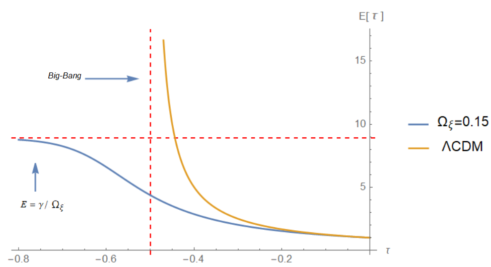
  Figure 1: Numerical behavior of $E(\tau)$, obtained from Eq. (II) at early-times, for $\Omega_{\Lambda_{0}}=10^{-6}$, $\Omega_{\xi_{0}}=0.15$ and $\gamma=4/3$. For a comparison, we also plotted the $\Lambda$CDM model obtained from Eq. (8).

• Early-time behavior of the exact solution: As it was discussed in Cruz et al. [a], if the condition (14) is fulfilled, then the solution represents a universe without singularity towards the past, as can be seen in Fig. 1, where numerically was found the behavior of $E$ as a function of $\tau$ from Eq. (II), with the values for the free parameters of $\gamma=4/3$ and $\Omega_{\xi_{0}}=0.15$. For these values, we are considered an early-time radiation domination era in a model only dominated by this dissipative radiation component and the CC, therefore, we consider the value of $\Omega_{\Lambda}=10^{-6}$ since the contribution of radiation is bigger than the DE component in this era. Note that the fulfillment of Eq. (14) implies the fulfillment of Eq. (12) which ensure a constant positive energy density. Even more, as it was discussed in Cruz et al. [a], the Ricci scalar is finite with the presence of viscosity, but we recovered the divergence when we neglect the dissipation. On the other hand, from Eq. (10) and Fig. 1 it can be seen that, if we take the limit $\Omega_{\xi_{0}}\rightarrow 0$, then $E\rightarrow\infty$, and the solutions tend to a model with a Big-Bang singularity. Therefore, for the condition given by Eq. (14), Eqs. (10) represent the asymptotic past behavior for the exact analytical solution (II).

In our study, this early-time behavior of the solution is of interest, in which the model is dominated by a radiation viscous component and a DE given by the CC, which is small but not negligible, leading to a solution without the initial Big-Bang singularity, with a behavior known as soft-Big Bang, describing a solution that starts in an eternal physical past time that comes from a static universe, avoiding a quantum regime for the space-time. In particular, we study the fulfillment of the near equilibrium condition, the mathematical stability, and the entropy production of the solution in order to obtain a suitable non-singular early-time viscous solution from the physical and mathematical point of view.

III Near equilibrium condition, mathematical stability and entropy production

III.1 Near equilibrium condition

The near equilibrium condition (1) is a consequence of the fact that Eckart’s theory is a relativistic thermodynamic theory out of the equilibrium, but close to this. According to Maartens in Maartens [a] and by the consideration of Eqs. (3), (5), and (6), which leads to

$$\frac{\ddot{a}}{a}=-\frac{1}{6}\left(\rho+3\left(p+\Pi\right)\right)+\frac{\Lambda}{3},$$ (15)

the condition to have an accelerated expansion ($\ddot{a}>0$) driven only by the negativeness of the viscous pressure $\Pi$ (i.e. $\Lambda=0$) drives to the condition

$$-\Pi>p+\frac{\rho}{3}.$$ (16)

A direct inspection of the previous result shows that the viscous pressure $\Pi$ is greater than the equilibrium pressure $p$ of the fluid, and then, the near equilibrium condition is not fulfilled. In other words, an accelerated expansion due only to the negativeness’s of the viscous pressure requires a theory beyond the near equilibrium regime assumed in Eckart’s theory Maartens [a]. Nevertheless, according to the authors in Cruz et al. [d], L. Herrera-Zamorano [b], Cruz et al. [b], the near equilibrium condition could hold in some regimes if one includes a positive CC. In this sense, the condition $\ddot{a}>0$ on Eq. (15) leads to

$$-\Pi>\frac{-2\Lambda}{3}+p+\frac{\rho}{3},$$ (17)

and the near equilibrium condition could be fulfilled because from Eq. (17) the viscous pressure $\Pi$ is not necessarily greater than the equilibrium pressure $p$ of the dissipative fluid. On the other hand, it is possible to rewrite the near equilibrium condition (1) in a dimensionless form, by the use of Eq. (6) and the EoS, leading to

$$l=\left|\frac{E(\tau)\Omega_{\xi_{0}}}{\gamma-1}\right|\ll 1.$$ (18)

Note that this last result shows that the behavior of $l$ as a function of time $\tau$ is driven by the behavior of the dimensionless Hubble parameter $E(\tau)$, and this condition is not satisfied when the solution has a initial singularity, where $E(\tau)\to\infty$. Nevertheless, for the early radiation dominant era, where the value of $\gamma$ is bigger than one, the last expression remains finite for a past eternal universe in which $E(\tau)\to const.$, indicating the possibility of fulfilling the near equilibrium condition. It is important to note that this result is independent of the inclusion of a CC because in a radiation domination era we need a decelerated expanding universe instead of an accelerated expanding one.

III.2 Mathematical stability

For mathematical stability, we study the behavior of the Hubble parameter under a small perturbation, i.e., we write

$$E_{\delta}(\tau)=E(\tau)+h(\tau),\,\,\,|h(\tau)|\ll E(\tau),$$ (19)

where $E(\tau)$ correspond to the unperturbed Hubble parameter in its dimensionless form, and $h(\tau)$ correspond to the small perturbation function. Introducing Eq. (19) in Eq. (7), we obtain the following differential equation, in our dimensionless notation, for $h(\tau)$:

$$h^{\prime}-\frac{9\Omega_{\xi_{0}}}{2}\left(E^{2}-\frac{2\gamma}{3\Omega_{\xi_{0}}}E-\frac{\Omega_{\Lambda_{0}}}{3}\right)h=0,$$ (20)

where “prime” denotes the derivative with respect to $\tau$. The above expression is a differential equation for the perturbation function $h(\tau)$ and describes the behavior of this perturbation with time $\tau$, i.e, for a mathematically stable solution to early times, we need to impose that $h(\tau\to-\infty)\to 0$.

III.3 Entropy production

The internal energy of a cosmic fluid and its physical three dimensional volume are given by $U=\rho V$ and $V=V_{0}a^{3}$ (where $V_{0}$ is the present-time volume), respectively. By the consideration of the the first law of thermodynamics equation

$$TdS=dU+pdV,$$ (21)

where $T$ and $S$ are the temperature and entropy of the cosmic fluid, respectively, we can find from Eq. (21) the Gibbs equation Maartens [b], Cruz et al. [b] given by

$$dS=-\left(\frac{\rho+p}{Tn^{2}}\right)dn+\frac{d\rho}{Tn},$$ (22)

where $n=N/V$ is the number of particle density. Also, we have the following integrability condition

$$\left[\frac{\partial}{\partial\rho}\left(\frac{\partial S}{\partial n}\right)_{\rho}\right]_{n}=\left[\frac{\partial}{\partial n}\left(\frac{\partial S}{\partial\rho}\right)_{n}\right]_{\rho},$$ (23)

that must hold on to the thermodynamical variables $\rho$ and $n$. Following this, we considered the thermodynamic assumption in which the temperature is a function of the number of particles density and the energy density, i.e., $T(n,\rho)$. With this, the integrability condition given by Eq. (23) become in Tamayo , Maartens [b], Cruz et al. [b]

$$n\frac{\partial T}{\partial n}+\left(\rho+p\right)\frac{\partial T}{\partial\rho}=T\frac{\partial p}{\partial\rho}.$$ (24)

In order to compare our result with the model without viscosity, we study the case of a perfect fluid and a viscous fluid separately.

For a perfect fluid, the particle four-current is given by $n^{\alpha}_{;\alpha}=0$, where the symbol “;” refers to covariant derivative, and together with the conservation equation, we have the following expressions for the particle density and the energy density, respectively:

$$\dot{n}+3Hn=\frac{\dot{N}}{N} = 0,$$ (25)

$$\dot{\rho}+3H(\rho+p) = 0.$$ (26)

Assuming also that the energy density depends on temperature and volume, i.e., $\rho(T,V)$ Tamayo , Cruz et al. [b], we have then the following relation:

$$\frac{d\rho}{da}=\frac{\partial\rho}{\partial T}\frac{dT}{da}+\frac{3n}{a}\frac{\partial\rho}{\partial n}.$$ (27)

It is possible to show, with the help of Eqs. (26), (27), and the EoS, that the temperature given by Eq. (24) will be directly proportional to the internal energy, i.e., $T\sim U$ Tamayo , Cruz et al. [b]. Note, from Eq. (22), together with Eqs. (25), (26), and the EoS, that the entropy production is equal to $dS=0$, a condition which implies that there is no entropy production in the cosmic expansion, and therefore, the fluid is adiabatic.

For a viscous fluid, in the framework of Eckart’s theory, the average four-velocity is chosen in a frame where there is no particle flux Weinberg and Dicke , Eckart . Therefore, in this frame, the expression $n^{\alpha}_{;\alpha}=0$ is still valid, and Eq. (25) doesn’t change. On the other hand, from Eqs. (4) and (5), we have the following conservation equation:

$$\dot{\rho}+3H(\rho+p+\Pi)=0,$$ (28)

which together with the Eq. (25) and the EoS, the Eq. (22) give us the following expression for entropy production Tamayo , Cruz et al. [e, b], given in a dimensionless form:

$$nT\frac{dS}{d\tau}={3E^{2}\Omega_{\xi_{0}}\rho}.$$ (29)

As we can see from the above expression, the entropy production in the viscous expanding universe is strictly positive, as long as the free parameters of the models are compatible with physical conditions like $\rho>0$, and is possible to obtain the behavior of a perfect fluid when $\Omega_{\xi_{0}}=0$.

IV Study of the exact solution to early-time

In this section, we study the exact solution given by the Eq. (II) under the condition (14) in terms of the fulfillment, at the same time, of the near equilibrium condition, the mathematical stability, and the positiveness of the entropy production. For that end, we focus our analysis on two defined early-time epochs of validity for the solution: (i) an arbitrary time for the radiation domination era in which $\tau=0$, $a=1$ and $E=1$, and (ii) the asymptotic soft-Big Bang era where $\tau\to-\infty$ and for which $E=\gamma/\Omega_{\xi_{0}}$.

IV.1 Near equilibrium condition

Here, we study Eq. (18) backward in time. Note that this condition can be rewritten as

$$E(\tau)\ll\frac{\gamma-1}{\Omega_{\xi_{0}}}=\frac{\gamma}{\Omega_{\xi_{0}}}-\frac{1}{\Omega_{\xi_{0}}},$$ (30)

an expression that tells us that as long as $E(\tau)$ be much smaller than $(\gamma-1)/\Omega_{\xi_{0}}$, then the solution must be near to the thermodynamic equilibrium. Considering then the first case in which $E(\tau=0)=1$, the condition (30) leads to

$$\Omega_{\xi_{0}}\ll\gamma-1,$$ (31)

which ensures that the theory is close to the thermodynamic equilibrium in the initial radiation domination era as long as $\Omega_{\xi_{0}}\ll 1/3$. It is important to note that, if we satisfy the previous expression, then, we will satisfy, at the same time, the condition (14) for which this past eternal solution hold. On the other hand, as time goes backward, then the solution increase asymptotically to the de Sitter-like solution given by (10), and therefore, for the soft-Big Bang era the near equilibrium condition (30) leads to

$$\gamma\ll\gamma-1,$$ (32)

i.e., the solution is far from the near equilibrium condition. In other words the near equilibrium condition can never be satisfied for $\gamma\geq 1/2$ (i.e., $p\geq-\rho/2$). Note that, in this case, and contrary to what happens in the case of an accelerated expanding universe, the inclusion of a positive CC constant could lead to the violation of the near equilibrium condition because a radiation domination era is characterized by a decelerated expanding universe ($\ddot{a}<0$) and, therefore, the inequality in the condition (17) changes. Nevertheless, the not inclusion of a CC implies abandoning all the good behaviors of the solution at late timesCruz et al. [b]. Therefore, the soft Big-Bang solution cannot hold the near equilibrium condition in the infinity past time. In this sense, the near equilibrium condition is an effective way to study the feasibility of the solution.

In order to study the limits where the near equilibrium condition holds in the common era of radiation, we consider in Eq. (30) the values of $\gamma=4/3$ and $\Omega_{\Lambda_{0}}=1\times 10^{-6}$, and we assume for simplicity that we are far from near equilibrium condition when $l=1$, i.e.,

$$E=\frac{1}{3\Omega_{\xi_{0}}}.$$ (33)

To be close to the near equilibrium condition, if we substitute the above value for the dimensionless Hubble parameter in (II), and the life-time for the radiation dominant era from Eq. (8), we will get from Eq. (II) a value for the viscosity of $\Omega_{\xi_{0}}=0.0080938$. Hence, we have the following restriction:

$$0<\Omega_{\xi_{0}}<0.0080938.$$ (34)

In Fig. 2 we display the near equilibrium condition for the fixed value of $\Omega_{\xi_{0}}=0.001$. At the beginning of the radiation domination era $(\tau=0$ and $E=1$), we obtained a value of $l=0.003$, according to the Eq. (18), and we are far from near equilibrium, according to Eq. (33), when $E=333.333$. The purple points represent the maximum and minimum values of $l$ in order to be close to the near equilibrium when $\gamma=4/3$, and the green line represents the evolutionary history in which we are near to thermodynamic equilibrium. The blue point represents the value when $E=235.704$, which represents the point where the Big Bang should occur if we consider the lifetime of the Universe according to Eq. (8) for the $\Lambda$CDM model in Eq. (II).

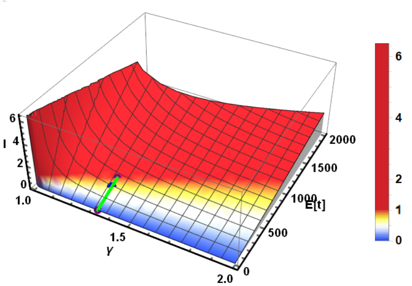
Figure 2: Behavior of $l$, given by Eq. (18), with respect to $\gamma$, and from $E=1$ (arbitrary initial radiation time) to $E=\gamma/\Omega_{\xi_{0}}$ (soft Big-Bang). The particular value of $\Omega_{\xi_{0}}=0.001$ is considered. The green line represents the near equilibrium history when $\gamma=4/3$, and the blue point represents the moment when the Big Bang occurs for the $\Lambda$CDM model.

Therefore, the solution can describe the radiation domination era of the $\Lambda$CDM model with a viscous radiation component that fulfills, for the entire era, the near equilibrium condition, but, for the infinite past time, when the solution tends to the soft Big-bang, we need to postulate that the solution holds beyond the near equilibrium condition.

IV.2 Mathematical stability

To analyze the mathematical stability, we use Eq. (20), changing the integration variable from $\tau$ to $E$, obtaining in our dimensional notation the expression

$$\frac{dh}{dE}=\frac{\left(\Omega_{\Lambda_{0}}\Omega_{\xi_{0}}+2\gamma E-3E^{2}\Omega_{\xi_{0}}\right)h}{\left(E^{2}-\Omega_{\Lambda_{0}}\right)\left(\gamma-E\Omega_{\xi_{0}}\right)},$$ (35)

whose integration leads to

$$h(E)=h_{i}\left(E\Omega_{\xi_{0}}-\gamma\right)\left(\Omega_{\Lambda_{0}}-E^{2}\right),$$ (36)

being $h_{i}$ and integration constant. If the condition given by Eq. (14) holds, then $E$ tends to $\gamma/\Omega_{\xi}$ backward in time (soft Big-Bang), and the perturbation function given by Eq. (36) goes to zero at this time, i.e, the solution is mathematically stable when $\tau\rightarrow-\infty$ or, in other words, the soft Big-Bang solution is mathematically stable. It is important to note that the solution (II) is also mathematically stable when $\tau\rightarrow\infty$ in which $E=\sqrt{\Omega_{\Lambda_{0}}}$ (de Sitter solution), as can be seen from Eq. (36).

We can find the maximum values for the perturbation function form Eq. (36), being obtained

$$E=\frac{\gamma\pm\sqrt{\gamma^{2}+3\Omega_{\xi_{0}}\Omega_{\Lambda_{0}}}}{3\Omega_{\xi_{0}}}.$$ (37)

From now, we only consider the positive sign, because the negative sign gives a value of $E<0$ which doesn’t occur for the entire cosmic evolution of the solution (II). In order to find some constraint in the cosmological parameters that ensure stability in the entire radiation era, we substitute Eq. (37) in (36), getting the following condition:

$$h = h_{i}\Big{|}\Big{(}\frac{2\gamma^{3}}{27\Omega^{2}_{\xi_{0}}}+\frac{2\gamma^{2}\sqrt{\gamma^{2}+3\Omega^{2}_{\xi_{0}}\Omega_{\Lambda_{0}}}}{27\Omega^{2}_{\xi_{0}}}$$ (38)

$$+ \frac{2}{9}\Omega_{\Lambda_{0}}\sqrt{\gamma^{2}+3\Omega^{2}_{\xi_{0}}\Omega_{\Lambda_{0}}}-\frac{2\gamma\Omega_{\Lambda_{0}}}{3}\Big{)}\Big{|}\ll E(\tau),$$

where $h_{i}$ is fixed considering that $h(E=1)=0.00001$. From Eq. (38), we can see that if $\Omega_{\xi_{0}}\rightarrow 0$, then $h\rightarrow\infty$ and we are far from the mathematical stability. This should not be a surprise because with very small values of $\Omega_{\xi_{0}}$ the solution tends to the $\Lambda$CDM model with Big-Bang singularity as was discussed in section II. For the radiation era, $\Omega_{\Lambda_{0}}$ has a small contribution to the total energy budget and, in addition, in order to be close to the near equilibrium condition, we need to fulfill the constraint given by Eq. (34), i.e., $\Omega_{\xi_{0}}$ must be small. We begin studying the stability when $H(t)$ is close to an arbitrary value of $H_{0}$, in the radiation dominant era. Therefore, we can approximate Eq. (38) as

$$h\approx\left|h_{i}\frac{4\gamma^{3}}{27\Omega^{2}_{\xi_{0}}}\right|<1.$$ (39)

For the radiation era, we have $\gamma=4/3$, and the above restriction in $\Omega_{\xi_{0}}$ gives us

$$0.00162387<\Omega_{\xi_{0}}<\frac{4}{3}.$$ (40)

In Fig. 3, we display the behaviour of the perturbation function $h$ as a function of the dimensionless Hubble parameter $E$, given by Eq. (36), for the fixed values of $\Omega_{\xi_{0}}=0.002$ and $\Omega_{\Lambda}=10^{-6}$. From Eq. (39), we obtain that the maximum value for $h$ is $0.659426$, and from Eq. (37), we can see that this value is obtained when $E=444.444$. Therefore, the solution (II) is stable for the usual radiation domination era. In the figure, the green line is given by Eq. (38) and represents the maximum points that can be obtained for the value of $h(E)$. We can also see one point in purple that represents the maximum value obtained for radiation ($\gamma=4/3$).

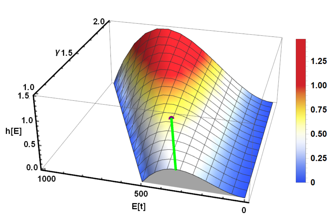
Figure 3: Behavior for $h$, given by Eq. (36), as a function of $\gamma$, and from $E=1$ (arbitrary initial radiation-time) to $E=\gamma/\Omega_{\xi}$ (soft Big-Bang). The values of $\Omega_{\Lambda}=10^{-6}$ and $\Omega_{\xi}=0.002$ are considered. The green line are given by Eq. (38), and the purple point represent the maximum value obtained for $\gamma=4/3$.

Finally, we can find a single constraint on $\Omega_{\xi_{0}}$ from Eqs. (34) and (40), given by

$$0.00162387<\Omega_{\xi_{0}}<0.0080938.$$ (41)

This single constraint allows us to satisfy both criteria, the near equilibrium condition, and the mathematical stability in the Hubble parameter, for the usual radiation era of the $\Lambda$CDM model.

IV.3 Temperature and entropy production

In order to evaluate the entropy production of the dissipative radiation component of the model from the Eq. (29), we first need to find their temperature from the Eq. (24). Rewriting the conservation Eq. (28) in the form

$$\frac{d\rho}{da}=-\frac{3\rho}{a}\left(\gamma-3H\xi_{0}\right),$$ (42)

we can rewrite Eq. (27) as

$$\rho\left(\gamma-3H\xi_{0}\right)=-\frac{a}{3}\frac{\partial\rho}{\partial T}\frac{dT}{da}-n\frac{\partial\rho}{\partial n}.$$ (43)

Then, from Eq. (24) and Eq. (5), we have

$$n\frac{\partial T}{\partial n}+\rho\left(\gamma-3H\xi_{0}\right)\frac{\partial T}{\partial\rho}=T\left[\left(\gamma-1\right)-3H\xi_{0}-3\xi_{0}\rho\frac{\partial H}{\partial\rho}\right],$$ (44)

which together with Eq. (43) leads to

$$\frac{dT}{T}=-3\frac{da}{a}\left[\left(\gamma-3H\xi_{0}\right)-1-3\xi_{0}\rho\frac{\partial H}{\partial\rho}\right].$$ (45)

By the use of Eqs. (2) and (42), we can rewrite the Eq. (45) in the the following form:

$$\frac{dT}{T}=\frac{d\rho}{\rho}\left[1-\frac{\left(\frac{2}{3}\sqrt{3\left(\rho+\Lambda\right)}+\xi_{0}\rho\right)}{\frac{2}{3}\sqrt{3\left(\rho+\Lambda\right)}\left(\gamma-\sqrt{3\left(\rho+\Lambda\right)}\xi_{0}\right)}\right].$$ (46)

Since we are considering the evolution of the solution (II) in an arbitrary time in the radiation domination era in which $E(\tau=0)=1$ to the past when $E(\tau\to-\infty)=\gamma/\Omega_{\xi_{0}}$, then, we integrate the Eq. (46) from $E=1$ to an arbitrary past-time $E(\tau<0)$, being obtained

$$\ln{\left(\frac{T}{T_{0}}\right)}=\ln\left(\frac{\rho}{\rho_{0}}\right)$$

$$-\frac{2\Omega_{\xi_{0}}\sqrt{\Omega_{\Lambda}}\left[\operatorname{arctanh}{\left(\frac{\sqrt{\Omega_{\Lambda_{0}}}}{E}\right)}-\operatorname{arctanh}{\left(\sqrt{\Omega_{\Lambda_{0}}}\right)}\right]}{\left(\gamma^{2}-\Omega_{\Lambda_{0}}\Omega^{2}_{\xi_{0}}\right)}+$$

$$\frac{\gamma\ln\left({\frac{\rho}{\rho_{0}}}\right)-\left[\gamma(2+\gamma)-\Omega_{\Lambda_{0}}\Omega^{2}_{\xi_{0}}\right]\ln{\left(\frac{\gamma-E\Omega_{\xi_{0}}}{\gamma-\Omega_{\xi_{0}}}\right)}}{\left(\gamma^{2}-\Omega_{\Lambda_{0}}\Omega^{2}_{\xi_{0}}\right)}.$$ (47)

On the other hand, integrating Eq. (42), with the help of Eq. (2), we obtain in our dimensionless notation the expression

$$\ln{a^{3}} = \frac{2\Omega_{\xi_{0}}\sqrt{\Omega_{\Lambda}}\left[\operatorname{arctanh}{\left(\frac{\sqrt{\Omega_{\Lambda_{0}}}}{E}\right)}-\operatorname{arctanh}{\left(\sqrt{\Omega_{\Lambda_{0}}}\right)}\right]}{\left(\gamma^{2}-\Omega_{\Lambda_{0}}\Omega^{2}_{\xi_{0}}\right)}$$ (48)

$$+ \frac{-\gamma\ln\left({\frac{\rho}{\rho_{0}}}\right)+2\gamma\ln{\left(\frac{\gamma-E\Omega_{\xi_{0}}}{\gamma-\Omega_{\xi_{0}}}\right)}}{\left(\gamma^{2}-\Omega_{\Lambda_{0}}\Omega^{2}_{\xi_{0}}\right)}.$$

With this last result, we can express the temperature from Eq. (47) of the dissipative radiation fluid as a function of the scale factor as follows

$$T=T_{0}\left(\frac{\rho}{\rho_{0}}\right)\left(\frac{\gamma-\Omega_{\xi_{0}}}{\gamma-E\Omega_{\xi_{0}}}\right){a^{-3}}.$$ (49)

We can see from Eq. (49) that when $E(\tau\rightarrow-\infty)$ the solution goes to the soft Big-Bang given by Eq. (10), and the temperature increase as long as the radiation fluid is compressed in the past infinity ($a\rightarrow 0$), until reaching a state where the energy density would be constant and given by Eq. (13). In this stage, the universe would be infinitely hotter since the expression for the temperature of the dissipative fluid given by Eq. (49) diverge, being this a reasonable behavior for which the solution would be far from the near equilibrium regime, as it was discussed in the section IV.1. It is important to note that, in this model, the temperature increases to infinity in the infinity past, whereas in the $\Lambda$CDM model the temperature is infinity in a finite pats time.

In Fig. 4, we display the numerical behavior of the temperature for the dissipative radiation fluid ($\gamma=4/3$) for the fixed values of $\Omega_{\Lambda_{0}}=10^{-6}$ and $\Omega_{\xi_{0}}=0.002$ (according to restriction (41)). The energy density of the dissipative radiation fluid is obtained from Eq. (48).

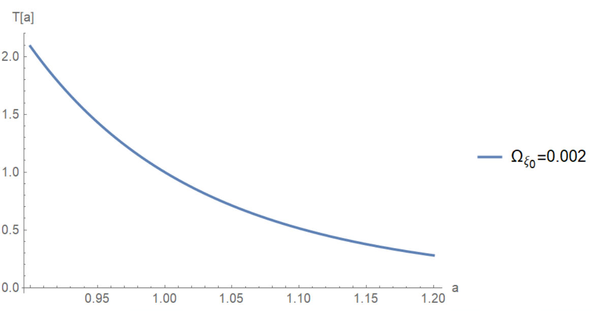
Figure 4: Behavior of the temperature of the dissipative radiation fluid ($\gamma=4/3$), given by Eq. (49), from $a=0.9$ to $a=1.20$ ($a=1$ represents an arbitrary time for the radiation domination era in which $\tau=0$ and $E=1$). The values of $\Omega_{\Lambda_{0}}=10^{-6}$ and $\Omega_{\xi_{0}}=0.002$ are considered.

With the temperature given by Eq. (49), we can calculate the entropy production from Eq. (29). By the use of Eq. (25) we have $n=n_{0}a^{3}$, and the entropy production for the dissipative radiation fluid is given by

$$\frac{dS}{d\tau}=\frac{3E^{2}\Omega_{\xi_{0}}\rho}{nT}=\frac{3E^{2}\rho_{0}\left(\gamma-E\Omega_{\xi_{0}}\right)\Omega_{\xi_{0}}}{n_{0}T_{0}\left(\gamma-\Omega_{\xi_{0}}\right)}.$$ (50)

Note that, in the infinite past, the solution (II) tends to the asymptotic soft Big-bang solution $E=\gamma/\Omega_{\xi_{0}}$ with null entropy production according to Eq. (50). This result is due to the asymptotic behavior of the fluid since, in this stage, the fluid will be fully compressed with a constant energy density given by Eq. (13) with no change in the micro-states of the system. Considering Eq. (41), then the entropy production for this radiation domination era ($\gamma=4/3$) would be positive and finite.

On the other hand, making use of Eq. (7) to rewrite Eq. (50), and making the integration over $E$, we will obtain in our dimensional notation the expresion

$$dS=\frac{-2\Omega_{\xi_{0}}\rho_{0}E^{2}dE}{n_{0}T_{0}\left(\gamma-\Omega_{\xi_{0}}\right)\left(E^{2}-\Omega_{\Lambda_{0}}\right)},$$ (51)

and then,

$$S(E) = S_{0}-\frac{2\rho_{0}}{n_{0}T_{0}\left(\gamma-\Omega_{\xi_{0}}\right)}\Big{\{}$$ (52)

$$+ \Omega_{\xi_{0}}\sqrt{\Omega_{\Lambda_{0}}}\ln\left[\left(\frac{\sqrt{\Omega_{\Lambda_{0}}}\Omega_{\xi_{0}}+\gamma}{\sqrt{\Omega_{\Lambda_{0}}}\Omega_{\xi_{0}}-\gamma}\right)\left(\frac{\sqrt{\Omega_{\Lambda_{0}}}-E}{\sqrt{\Omega_{\Lambda_{0}}}+E}\right)\right]$$

$$+ E\Omega_{\xi_{0}}-{\gamma}\Big{\}}.$$

From the above expression, the constraint for a positive energy density for the soft Big-bang solution given by Eq. (12) ensures a real value for entropy since in the logarithm term $E$ is greater than $\sqrt{\Omega_{\Lambda_{0}}}$. Note that, for the infinity past when $E\rightarrow\gamma/\Omega_{\xi_{0}}$, we get $S=S_{0}$, i.e. a constant entropy. In Fig. 5 is represented the numerical behavior of the entropy for the dissipative radiation fluid ($\gamma=4/3$) for $\Omega_{\Lambda_{0}}=10^{-6}$ and $\Omega_{\xi_{0}}=0.002$ (according to restriction Eq. (41)), for the particular initial value of $S_{0}=0$. We can see that the same condition that satisfies the near equilibrium condition and the mathematical stability of the Hubble parameter are compatible with a positive entropy that increase with the universe expansion from $E=\gamma/\Omega_{\xi_{0}}=666.7$ (soft-Big Bang) to $E=1$ (arbitrary initial time in the radiation domination era).

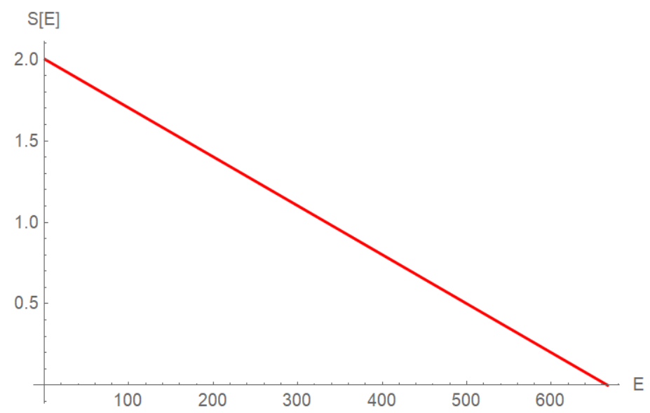
Figure 5: Behavior of the entropy for the dissipative radiation fluid ($\gamma=4/3$), given by Eq. (52), from $E=1$ (arbitrary initial time in the radiation domination era) to $E=\gamma/\Omega_{\xi_{0}}$ (soft Big-Bang). The values of $\Omega_{\Lambda_{0}}=10^{-6}$ and $\Omega_{\xi_{0}}=0.002$ are considered.

V Discussion

We have studied throughout this work the near equilibrium condition, the mathematical stability of the Hubble parameter, and the entropy production of a bulk viscous model previously found in Cruz et al. [a], within the framework of Eckart’s theory, in an early-time era of the cosmic evolution. The model represents a universe filled with a dissipative radiation component, where the bulk viscosity is proportional to their energy density according to the expression $\xi=\xi_{0}\rho$, and a positive CC whose contribution to the total energy density budget is small but not negligible. This model is characterized by a past eternal behavior known as “soft-Big Bang”, with an asymptotic solution given by Eq. (10), as long as the condition $\Omega_{\xi_{0}}<\gamma$ holds, which also implies the fulfillment of the condition (12), i.e., this asymptotic behavior has a constant and positive energy density in the infinity past time, contrary to the infinity energy density obtained in the $\Lambda$CDM model, which occurs in a finite time. In addition, this model follows very close to the $\Lambda$CDM behavior for small values of dissipation ($\Omega_{\xi}\rightarrow 0$), as we can see in Fig. 1.

We have shown in section IV.1 that, for a viscous radiation component, where $\gamma$ is bigger than one, the behavior of the expression for the near equilibrium condition ($l$) is driven by the behavior of the dimensionless Hubble parameter $E(\tau)$, according to Eq. (18), and, as a long as the condition (14) is satisfied, $E(\tau)$ tends asymptotically to the soft-Big bang solution (10) and, therefore, the near equilibrium condition (18) remains finite for this past eternal universe. From Fig. 2, we can see that this model can describe the radiation domination era of the $\Lambda$CDM model and, for the entire era, the near equilibrium condition is fulfilled as a long as the constraint for the bulk viscous coefficient given by Eq. (34) is satisfied. Nevertheless, for the infinite past time, when the solution tends to the soft-Big bang, the near equilibrium condition is not satisfy. Thus, we examine the limits within which the solution remains viable in terms of the near equilibrium condition.

In section IV.2, we have shown that a small perturbative function in the mathematical expression for the Hubble parameter solution (II) is stable for $\gamma=4/3$, as long as we satisfy the condition given by Eq. (40), as we can see in Fig. 3. Therefore, we can have a single constraint in $\Omega_{\xi_{0}}$ to satisfy both criteria, the near equilibrium condition and the stability in the Hubble parameter which is given by Eq. (41).

The temperature and the entropy production for the viscous radiation fluid were studied in section IV.3. The temperature is given by Eq. (49), and in the infinity past ($a\rightarrow 0$), the fluid is compressed to a constant energy density given by Eq. (13), where the temperature diverges and starts to decrease during his expansion as we can see in Fig. 4. Therefore, as long as the temperature increase to infinity, we will start to be far from near equilibrium condition as is displayed in Fig. 2. The advantage of this model is that the temperature is not infinity in a finite time like in the $\Lambda$CDM model and, therefore, the presence of viscosity together with a positive CC acts as a modulator in the near equilibrium process before the temperature starts to be extremely high. For the entropy production, this is strictly positive, and when we go backward in time the fluid starts to compress as long as the scale factor goes to zero, getting a constant energy density given by Eq. (13). Therefore, the entropy production goes to zero during this compression of the fluid, and the restriction (12) appears automatically within the expression of the logarithm in (52), to ensure the real value of the entropy. Also, the consideration of near equilibrium regime together with mathematical stability implies the condition (41), and with this constraint, the entropy is positive and well behaved, as we can see in Fig. 5.

Therefore, the solution given by Eq. (II) can describe the entire radiation era of the $\Lambda$CDM model with a viscous radiation component instead of a perfect radiation fluid, satisfying at the same time the near equilibrium condition, the positiveness of the entropy production and the solution is mathematically stable, as a long as the conditions described before holds. The principal characteristic of the solution is to avoid the initial Big Bang singularity, although the solution behaves very similar to the $\Lambda$CDM model, in an asymptotic past eternal behavior known as soft-Big Bang.

References

- et. al [a] N. Aghanim et. al. Planck 2018 results. vi. cosmological parameters. A & A 641, A6 (2020), a.
- et. al [b] Shadab Alam et. al. The clustering of galaxies in the completed sdss-iii baryon oscillationspectroscopic survey: cosmological analysis of the dr12 galaxy sample. Mon.Not.Roy.Astron.Soc. 470 (2017) 3, 2617-2652, b.
- et. al [c] G. Hinshaw et. al. Nine-year wilkinson microwave anisotropy probe (wmap) observations: Cosmological parameter results. Astrophys.J.Suppl. 208 (2013) 19, c.
- [4] Joseph Ryan Shulei Cao and Bharat Ratra. Using pantheon and des supernova, baryon acoustic oscillation, and hubble parameter data to constrain the hubble constant, dark energy dynamics, and spatial curvature. MNRAS, 504, 300-310 (2021).
- et. al [d] S. Perlmutter et. al. Measurements of and from 42 High-Redshift Supernovae. Astrophys.J.517:565-586,1999, d.
- [6] Marc Davis, George Efstathiou, Carlos S. Frenk, and Simon D.M. White. The evolution of large scale structure in a universe dominated by cold dark matter. Astrophys.J. 292 (1985) 371-394.
- [7] Steven Weinberg and R. H. Dicke. Gravitation and Cosmology: Principles and Applications of the General Theory of Relativity. ISBN 9780471925675, 9780471925675.
- [8] Georges Lemaitre. The beginning of the world from the point of view of quantum theory. Nature 127 (1931) 706.
- Hawking and Ellis [2011] S. W. Hawking and G. F. R. Ellis. The Large Scale Structure of Space-Time. Cambridge Monographs on Mathematical Physics. Cambridge University Press, 2 2011. ISBN 978-0-521-20016-5, 978-0-521-09906-6, 978-0-511-82630-6, 978-0-521-09906-6. doi: 10.1017/CBO9780511524646.
- Cruz et al. [a] Norman Cruz, Esteban González, and José Jovel. Singularities and soft-big bang in a viscous cdm model. Phys. Rev. D 105, 024047, a.
- [11] E. Rebhan. ’soft bang’ instead of ’big bang’: Model of an inflationary universe without singularities and with eternal physical past time. Astron.Astrophys. 353 (2000) 1-9.
- [12] E. Elbaz M. Novello. Soft big bang model induced by nonminimal coupling. Nuovo Cim.B 109 (1994) 741-746.
- [13] Rosen N. Israelit M. A singularity-free cosmological model in general relativity. Astrophys. J. 342, 627 (1989).
- [14] Priester W. Blome H.J. Big bounce in the very early universe. Astron. Astrophys. 250, 43 (1991).
- [15] Christos G. Tsagas George F.R. Ellis, Jeff Murugan. The emergent universe: An explicit construction. Class.Quant.Grav.21:233-250,2004.
- [16] George F. R. Ellis and Roy Maartens. The emergent universe: Inflationary cosmology with no singularity. Class. Quant. Grav.21:223-232,2004.
- [17] Alexei A. Starobinsky. A new type of isotropic cosmological models without singularity. Phys.Lett.B 91 (1980) 99-102, Adv.Ser.Astrophys.Cosmol. 3 (1987) 130-133.
- [18] T. Singh, R. Chaubey, and Ashutosh Singh. Bouncing cosmologies with viscous fluids. Astrophys Space Sci 361, 106 (2016).
- [19] Esteban González Felipe Contreras, Norman Cruz. Generalized equations of state and regular universes. J.Phys.Conf.Ser. 720 (2016) 1, 012014.
- [20] Felipe Contreras, Norman Cruz, Emilio Elizalde, Esteban González, and Sergei Odintsov. Linking little rip cosmologies with regular early universes. Phys.Rev.D 98 (2018) 12, 123520.
- Mukherjee et al. [2005] S. Mukherjee, B. C. Paul, S. D. Maharaj, and A. Beesham. Emergent universe in starobinsky model. 5 2005.
- [22] George L. Murphy. Big-bang model without singularities. Phys.Rev.D 8 (1973) 4231-4233.
- [23] M. Heller, Z. Klimek, and L. Suszycki. Imperfect fluid friedmannian cosmology. Astrophysics and Space Science, Volume 20, Issue 1, pp.205-212.
- [24] I. Brevik and G. Stokkan. Viscosity and matter creation in the early universe. Astrophysics and Space Science volume 239, pages89–96 (1996).
- [25] Winfried Zimdahl and Diego Pavón. Cosmology with adiabatic matter creation. Int.J.Mod.Phys.D 3 (1994) 327-330.
- [26] Gyan Prakash Singh and Aroonkumar Beesham. Bulk viscosity and particle creation in brans - dicke theory. Australian Journal of Physics 52(6):1039-1049.
- [27] Mehdi Eshaghi, Nematollah Riazi, and Ahmad Kiasatpour. Bulk viscosity and particle creation in the inflationary cosmology. arXiv:1504.07774.
- [28] Iver Brevik, Øyvind Grøn, Jaume de Haro, Sergei D. Odintsov, and Emmanuel N. Saridakis. Viscous cosmology for early- and late-time universe. Int.J.Mod.Phys. D26 (2017) 1730024.
- [29] Diego Pavon Luis P. Chimento, Alejandro S. Jakubi. Stability of inflationary solutions driven by a changing dissipative fluid. Class.Quant.Grav. 16 (1999) 1625-1635.
- [30] Kazuharu Bamba and Sergei D. Odintsov. Inflation in a viscous fluid model. arXiv:1508.05451.
- [31] Norman Cruz Miguel Cruz and Samuel Lepe. Accelerated and decelerated expansion in a causal dissipative cosmology. Phys. Rev. D 96, 124020 (2017).
- [32] R. de Sa Ribeiro J.C. Fabris, S.V.B. Goncalves. Bulk viscosity driving the acceleration of the universe. Gen.Rel.Grav.38:495-506,2006.
- Arturo Avelino [a] Ulises Nucamendi Arturo Avelino. Can a matter-dominated model with constant bulk viscosity drive the accelerated expansion of the universe? JCAP 0904:006,2009, a.
- Arturo Avelino [b] Ulises Nucamendi Arturo Avelino. Exploring a matter-dominated model with bulk viscosity to drive the accelerated expansion of the universe. JCAP 1008:009,2010, b.
- [35] Athira Sasidharan and Titus K. Mathew. Bulk viscous matter and recent acceleration of the universe. EPJ C 75 348 2015.
- [36] Jerin Mohan N D, Athira Sasidharan, and Titus K Mathew. Bulk viscous matter and recent acceleration of the universe based on causal viscous theory. The European Physical Journal C volume 77, Article number: 849 (2017).
- [37] A. Hernández Almada, Miguel A. García Aspeitia, M. A. Rodríguez-Meza, and V. Motta. A hybrid model of viscous and chaplygin gas to tackle the universe acceleration. arXiv:2103.16733.
- [38] Shin’ichi Nojiri and Sergei D. Odintsov. Inhomogeneous equation of state of the universe: Phantom era, future singularity and crossing the phantom barrier. Phys.Rev.D72:023003,2005.
- [39] S. Capozziello, V.F. Cardone, E. Elizalde, S.Nojiri, and S. D.Odintsov. Observational constraints on dark energy with generalized equations of state. Phys.Rev.D73:043512,2006.
- L. Herrera-Zamorano [a] A. Hernández-Almada L. Herrera-Zamorano, Miguel A. García-Aspeitia. Constraints and cosmography of cdm in presence of viscosity. Eur.Phys.J.C 80 (2020) 7, 637, a.
- [41] John D. Barrow Baojiu Li. Does bulk viscosity create a viable unified dark matter model? Phys.Rev.D79:103521,2009.
- [42] W. Zimdahl W.S. Hipólito-Ricaldi, H.E.S. Velten. Viscous dark fluid universe. Phys.Rev.D82:063507,2010.
- [43] Titus K Mathew Athira Sasidharan. Phase space analysis of bulk viscous matter dominated universe. JHEP 1606 (2016) 138.
- Norman Cruz [a] Guillermo Palma Norman Cruz, Esteban González. Exact analytical solution for an israel–stewart cosmology. Gen.Rel.Grav. 52 (2020) 6, 62, a.
- Norman Cruz [b] Guillermo Palma Norman Cruz, Esteban González. Testing dissipative dark matter in causal thermodynamics. Mod.Phys.Lett.A 36 (2021) 06, 2150032, b.
- Ganguly and Quintin [2022] Chandrima Ganguly and Jerome Quintin. Microphysical manifestations of viscosity and consequences for anisotropies in the very early universe. Phys. Rev. D, 105(2):023532, 2022. doi: 10.1103/PhysRevD.105.023532.
- Belinski [2013] V. A. Belinski. Stabilization of the friedmann big bang by the shear stresses. Phys. Rev. D, 88:103521, Nov 2013. doi: 10.1103/PhysRevD.88.103521. URL https://link.aps.org/doi/10.1103/PhysRevD.88.103521.
- Ganguly and Bruni [2019] Chandrima Ganguly and Marco Bruni. Quasi-Isotropic Cycles and Nonsingular Bounces in a Mixmaster Cosmology. Phys. Rev. Lett., 123(20):201301, 2019. doi: 10.1103/PhysRevLett.123.201301.
- [49] Carl Eckart. The thermodynamics of irreversible processes. iii. relativistic theory of the simple fluid. Phys. Rev. 58, 919 (1940).
- [50] L. D. Landau and E. M. Lifshitz. Fluid Mechanics Volume 6, (1959).
- [51] Werner Israel. Nonstationary irreversible thermodynamics: A causal relativistic theory. Annals Phys. 100 (1976) 310-331.
- [52] Ingo Muller. Zum paradoxon der warmeleitungstheorie. Z.Phys. 198 (1967) 329-344.
- Israel and Stewart [a] W. Israel and J. M. Stewart. Transient relativistic thermodynamics and kinetic theory. Annals Phys. 118 (1979) 341-372, a.
- Israel and Stewart [b] W. Israel and J. M. Stewart. On transient relativistic thermodynamics and kinetic theory. ii. R. Soc. Lond. A. 357,59-75 (1977), b.
- Maartens [a] R. Maartens. Dissipative cosmology. Class.Quant.Grav. 12 (1995) 1455-1465, a.
- [56] A. Hernández-Almada. Cosmological test on viscous bulk models using hubble parameter measurements and type ia supernovae data. Eur.Phys.J.C 79 (2019) 9, 751.
- [57] George M. Fuller James R. Wilson, Grant J. Mathews. Bulk viscosity, decaying dark matter, and the cosmic acceleration. Phys.Rev.D75:043521,2007.
- [58] Jinwen Hu and Huan Hu. Viscous universe with cosmological constant. Eur.Phys.J.Plus 135 (2020) 9, 718.
- [59] Norman Cruz Mauricio Cataldo and Samuel Lepe. Viscous dark energy and phantom evolution. Phys.Lett.B619:5-10,2005.
- [60] I. Brevik and O. Gorbunova. Dark energy and viscous cosmology. Gen.Rel.Grav. 37 (2005) 2039-2045.
- Cruz et al. [b] Norman Cruz, Esteban González, and Jose Jovel. Study of a viscous wdm model: Near equilibrium condition, entropy production, and cosmological constraints. arXiv:2202.02362 [gr-qc], b.
- Cruz et al. [c] Miguel Cruz, Norman Cruz, Esteban González, and Samuel Lepe. Testing a non linear solution of the Israel-Stewart theory with supernovae. arXiv:2109.08823 [gr-qc], c.
- Cruz et al. [d] Norman Cruz, Esteban González, Samuel Lepe, and Diego Sáez-Chillón Gómez. Analysing dissipative effects in the cdm model. JCAP 12 (2018) 017, d.
- L. Herrera-Zamorano [b] Miguel A. García-Aspeitia L. Herrera-Zamorano, A. Hernández-Almada. Constraints and cosmography of cdm in presence of viscosity. EPJC 80, 637 (2020), b.
- [65] T. Padmanabhan and S. Chitre. Viscous universes. Phys. Lett. A 120, 433 (1987).
- [66] Shin’ichi Nojiri, Sergei D. Odintsov, and Shinji Tsujikawa. Properties of singularities in (phantom) dark energy universe. Phys.Rev.D71:063004,2005.
- [67] Prado Martín-Moruno Mariam Bouhmadi-López, Claus Kiefer. Phantom singularities and their quantum fate: general relativity and beyond—a cantata cost action topic. Gen.Rel.Grav. 51 (2019) 10, 135.
- [68] David Tamayo. Thermodynamics of viscous dark energy. arXiv:2006.14153 [gr-qc].
- [69] O. Cornejo-Pérez and J. A. Belinchón. Exact solutions of a flat full causal bulk viscous frw cosmological model through factorization. International Journal of Modern Physics D, Vol. 22, No. 6 (2013) 1350031.
- Cruz et al. [e] Miguel Cruz, Norman Cruz, and Samuel Lepe. Phantom solution in a non-linear israel–stewart theory. Phys. Lett. B 769, 159 (2017), e.
- Maartens [b] Roy Maartens. Causal thermodynamics in relativity. astro-ph/9609119, b.
- [72] J. Salmonson W.A. Hiscock. Dissipative boltzmann-robertson-walker cosmologies. Phys.Rev.D 43 (1991) 3249-3258.
- [73] D. Jou D. Pavon, J. Bafaluy. Causal friedmann-robertson-walker cosmology. Class.Quant.Grav. 8 (1991) 347-360.
- Cruz et al. [f] Miguel Cruz, Samuel Lepe, and Sergei D. Odintsov. Thermodynamically allowed phantom cosmology with viscous fluid. Phys. Rev. D 98, 083515 (2018), f.
- [75] N.D. Jerin Mohan, P.B. Krishna, Athira Sasidharan, and Titus K. Mathew. Dynamical system analysis and thermal evolution of the causal dissipative model. arXiv:1807.04041 [gr-qc].
- [76] Titus K Mathew, Aswathy M B, and Manoj M. Cosmology and thermodynamics of flrw universe with bulk viscous stiff fluid. Eur.Phys.J.C 74 (2014) 99, 3188.
- [77] I. Brevik and A. V. Timoshkin. Thermodynamic aspects of entropic cosmology with viscosity. Int. J. Mod. Phys. D 30, 2150008 (2021).
- [78] Titus K Mathew Jerin Mohan N D. On the feasibility of truncated israel-stewart model in the context of late acceleration. Class.Quant.Grav. 38 (2021) 14, 145016.
- [79] Iver Brevik. Viscosity-induced crossing of the phantom barrier. Entropy, Vol. 17, pp. 6318-6328 (2015).
- [80] W. de Sitter. Einstein’s theory of gravitation and its astronomical consequences, third paper. Mon.Not.Roy.Astron.Soc. 78 (1917) 3-28.