A general framework for multi-step ahead adaptive conformal heteroscedastic time series forecasting

Abstract

This paper introduces a novel model-agnostic algorithm called adaptive ensemble batch multi-input multi-output conformalized quantile regression (AEnbMIMOCQR) that enables forecasters to generate multi-step ahead prediction intervals for a fixed pre-specified miscoverage rate $\alpha$ in a distribution-free manner. Our method is grounded on conformal prediction principles, however, it does not require data splitting and provides close to exact coverage even when the data is not exchangeable. Moreover, the resulting prediction intervals, besides being empirically valid along the forecast horizon, do not neglect heteroscedasticity. AEnbMIMOCQR is designed to be robust to distribution shifts, which means that its prediction intervals remain reliable over an unlimited period of time, without entailing retraining or imposing unrealistic strict assumptions on the data-generating process. Through methodically experimentation, we demonstrate that our approach outperforms other competitive methods on both real-world and synthetic datasets. The code used in the experimental part and a tutorial on how to use AEnbMIMOCQR can be found at the following GitHub repository: https://github.com/Quilograma/AEnbMIMOCQR.

List of symbols

Notation	Description
$\mathcal{A}$	arbitrary regression algorithm (e.g., lightGBM)
$x$	a scalar
$\bm{x}$	a vector
$\bm{X}$	a tensor or random vector
$\alpha$	miscoverage rate, between 0 and 1
$\alpha_{t}$	miscoverage rate, between 0 and 1 at the t-th timestep.
$\bm{\epsilon}$	set of non-conformity scores
Quantile($\bm{\epsilon}$; $1-\alpha$)	$1-\alpha$ quantile of $\bm{\epsilon}$
$C_{1-\alpha}(\bm{x_{n}})$	oracle $1-\alpha$ prediction interval on input $\bm{x_{n}}$
$\hat{C}_{1-\alpha}^{(t)}(\bm{x_{n}})$	estimated $1-\alpha$ prediction interval on input $\bm{x_{n}}$ at the t-th timestep
$Q_{\tau}(\bm{x})$	population conditional quantile for $\tau\in(0,1)$ on input $\bm{x}$
$\hat{Q}_{\tau}(\bm{x})$	conditional quantile estimate for $\tau\in(0,1)$ on input $\bm{x}$
$y_{t,h}$	observation at the t-th timestep for the h-th horizon
$X$	Random variable
$\mathbbm{1}$	Indicator function

1 Introduction

Recent advances in time series forecasting research have been driven by the increasing demand for higher forecast accuracy in complex settings, as set by modern big data applications (Das et al., 2023; Masini et al., 2023). While considerable effort has been dedicated to identifying the most effective approaches, with the widely recognized M forecasting competition, initiated in 1982 (Makridakis et al., 1982), serving as a arena for these breakthroughs, quantifying the uncertainty of such predictions has received diminished attention. Indeed, the inclusion of prediction intervals (PIs) began to be considered in forecasting competitions only from the M4 competition (Makridakis et al., 2020) onward. Another example of this discrepancy was observed in the M5 forecasting competitions. The M5 "Accuracy" competition (Makridakis et al., 2022a), which centered on optimizing point predictions, garnered significant interest and participation, with a staggering $7,092$ participants vying for top honors. In stark contrast, the M5 "Uncertainty" competition (Makridakis et al., 2022b), which aimed to assess the quality of estimated conditional quantiles, drew considerably less attention, involving only $1,137$ participants despite offering the same prize incentives.

Nevertheless, this seemingly diminished interest does not align with the actual relevance of probabilistic forecasting, which plays a pivotal role in numerous high-stakes domains, including finance (Fatouros et al., 2023), healthcare planning (Rostami-Tabar et al., 2023; Taylor & Taylor, 2023), energy (Cramer et al., 2023; Wang et al., 2022), and urban planning (Du et al., 2022; Qian et al., 2023), urging a greater focus on the topic. Probabilistic forecasting enables decision-makers to improve their decision-making by incorporating uncertainty, which is overlooked by point predictions. A common form of probabilistic forecast that we will delve into is a PI, which defines a specific range within which the actual future value is anticipated to lie, with a predetermined level of probability (e.g., 0.9). It differs from a confidence interval (Heskes, 1996) in that it takes into consideration both aleatory and epistemic uncertainties (Der Kiureghian & Ditlevsen, 2009).

While the advantages of PIs concerning informed decision-making are undeniable, their construction is anything but straightforward as time series are non i.i.d.. A recent paper (Xu & Xie, 2023) alluded to the need for a distribution-free framework that generates PIs for time series data, along with provable guarantees for interval coverage and model-agnosticity properties so that it can be wrapped around complex and flexible models such as lightGBM (Ke et al., 2017) that do not have an inherent method for generating PIs. In addition to the aforementioned criteria, a recent study (Dewolf et al., 2023a) draws out attention to the importance of PIs which handle heteroscedasticity. Bellow, we outline all properties this framework should comply with:

1. Mitigating the reliance on strict distributional assumptions;

2. Ensuring the validity of the generated PIs non-asymptotically;

3. Handling heteroscedasticity;

4. Ability to generate PIs for an arbitrary forecast horizon;

5. Model-agnosticity;

6. Minimizing the width of the generated PIs;

7. Reliability under distribution shift without entailing retraining.

In this paper, we embrace the challenge of presenting a framework designed to comprehend all of the aforementioned properties. Specifically, for an arbitrary forecast horizon $H$ we seek to ensure validity step-wise in the sense of (1), where $y_{t+h}$ is the unknown h-step ahead, $[\hat{y}_{t+h}^{L},\hat{y}_{t+h}^{U}]$ is the generated h-step ahead PI, and $\alpha\in(0,1)$ is the so-called miscoverage rate.

$$\mathbb{P}\{y_{t+h}\in[\hat{y}_{t+h}^{L},\hat{y}_{t+h}^{U}]\}=1-\alpha,\quad\forall h\in\{1,2...,H\}$$ (1)

1.1 Defining quality in prediction intervals

We will now delve into establishing the key attributes that constitute a high-quality PI, not exclusively tied to time series forecasting, but more generally any regression task. To this end, consider an unseen pair of covariates and target, denoted as $(\bm{x_{n+1}},y_{n+1})$; the foremost and arguably most crucial requirement that a high-quality PI should meet is validity, as outlined in Definition (1). It refers to the alignment between the desired and observed nominal coverage. A valid, sometimes also referred to as calibrated PI, ensures the specified nominal coverage—neither more nor less. For instance, for a 90% PI, around 90% of real observations should fall within. Another requirement is sharpness. A sharp PI is as narrower as possible to be informative. Moreover, a frequently overlooked yet essential criterion that PIs should also comply with is the ability to handle heteroscedasticity. Heteroscedasticity occurs when the error variance exhibits variation across the covariates space. A clear understanding of the distinction between marginal and conditional coverage is vital in order to grasp why marginally valid PIs may not be sufficient. Essentially, conditionally valid PIs adapt to the varying error variance in the covariates space, as stipulated in Definition (2). To help comprehension of these concepts, two plots, Figures 2 and 2, are presented, pointing the differences between these two types of PIs. While in Figure 2, the PIs adapt to the local uncertainty of the given input, in Figure 2, they fail to do so. Additionally, ensuring conditional coverage implies that miscoverage of the target variable is equally likely to occur across the covariates space. This becomes clearer if we increase $\alpha$ from $0.01$ to $0.1$, as shown in Figures 5 and 5, where we notice that in Figure 5 the ratio of miscoverage for $x\geq 40$ is much greater in comparison to $x<40$.

Thinking in a real-world setting where $x$ could represent a person’s age, deploying PIs as depicted in Figure 5 would raise severe ethical concerns in practice, despite satisfying Definition (1).

Definition 1 (Marginal validity (also known as marginal coverage)).

A PI is termed valid if for an unseen pair of covariates and target $(\bm{x_{n+1}},y_{n+1})$

$$\mathbb{P}\left\{y_{n+1}\in\hat{C}_{1-\alpha}(\bm{x_{n+1}})\right\}=1-\alpha$$ (2)

Definition 2 (Conditional validity (also known as conditional coverage)).

A PI is termed conditional valid if for an unseen pair of covariates and target $(\bm{x_{n+1}},y_{n+1})$

$$\mathbb{P}\left\{y_{n+1}\in\hat{C}_{1-\alpha}(\bm{x_{n+1}})|\bm{X_{n+1}}=\bm{x_{n+1}}\right\}=1-\alpha.$$ (3)

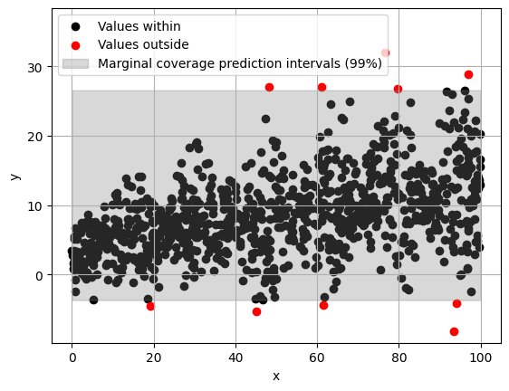
Figure 1: Marginally valid PIs for $\alpha=0.01$.

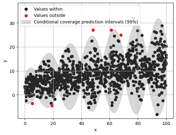
Figure 2: Conditionally valid PIs for $\alpha=0.01$.

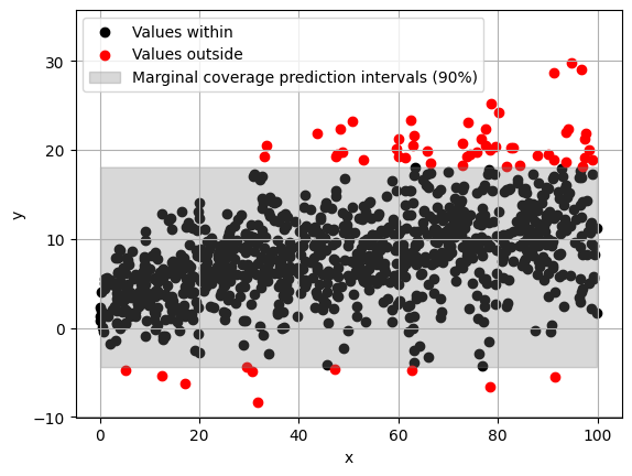
Figure 3: Marginally valid PIs for $\alpha=0.1$.

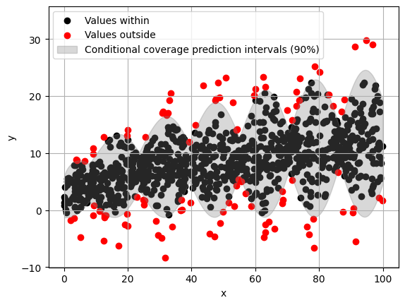
Figure 4: Conditionally valid PIs for $\alpha=0.1$.

Figure 5: *

Data generated according to $y=2+\sqrt{x}+\epsilon(x)$, where $\epsilon(x)=\mathcal{N}(0,2+|0.6\sqrt{x}\cos{0,0.2x}|)$ is an heteroscedastic aleatory noise and $x\in[0,100]$. A total of 1000 observations are present in each plot.

1.2 Literature review

Selecting the right approach to produce multi-step ahead PIs can be strenuous given the multitude of available approaches (Tyralis & Papacharalampous, 2022; Chatfield, 2001). Certain traditional methods have an in-built theoretical way to do so (Brockwell & Davis, 2002; Cochrane, 2005; Hyndman & Athanasopoulos, 2018). Nevertheless, their applicability is constrained by the reliance on robust parametric distributional assumptions. For example, PIs generated by autoregressive integrated moving average (ARIMA) are based on the premises of linearity, independence of residuals, homoscedasticity, normality, and stationarity after differencing, dissuading numerous practitioners from applying these methods in practical, real-world scenarios, primarily because of the formidable task of confirming these assumptions, which are seldom fulfilled. Employing these methods without proper verification is even more detrimental, as it most likely results in unreliable PIs.

In the M5 UQ competition (Makridakis et al., 2022b), one of the significant findings was that winning teams utilized simple machine learning (ML) models leveraging their inherent flexibility. Consequently, an advisable direction is to prioritize model-agnostic UQ methods, capable of encompassing a wide array of statistical models, particularly ML-based. These comprehend bootstrapping (Hongyi Li & Maddala, 1996; Flores-Agreda & Cantoni, 2019), deep ensembles (Lakshminarayanan et al., 2017), dropout (Gal & Ghahramani, 2016), empirical (Lee & Scholtes, 2014), Bayesian (Kwon et al., 2020; Harrison & Stevens, 1976; Gelman et al., 1995), Gaussian processes (Williams & Rasmussen, 1995), and quantile regression (QR) (Koenker & Hallock, 2001; Koenker, 2017). However, it is crucial to note that, in isolation, these methods generally do not consistently achieve validity, as demonstrated in a comprehensive independent experiment (Dewolf et al., 2023b). The authors of the aforementioned experiment, attribute this inconsistency between the desired and actual out-of-sample nominal coverage to the violation of certain assumptions that are inherent to some classes of methods. To overcome this limitation, the authors promote (CP) (Shafer & Vovk, 2008; Fontana et al., 2023; Angelopoulos & Bates, 2023) as a general calibration procedure for methods that deliver poor results without a calibration step.

Unlike the aforementioned methods, CP ensures marginal coverage in finite samples in a distribution-free manner under the mild assumption of exchangeability, a slightly weaker assumption compared to i.i.d., that is already implicit while training most statistical models. Despite this advantage, PIs built uniquely from CP may have fixed or weakly varying width regardless of the error variance input-wise (Foygel Barber et al., 2021; Johansson et al., 2014; Papadopoulos & Haralambous, 2011). To address this limitation, a method called conformalized quantile regression (CQR) (Romano et al., 2019) was proposed. CQR employs CP along with QR to correct its predictive bands, inheriting the most attractive features of both, resulting in valid PIs that account for the present heteroscedasticity to a certain extend.

In time series data, the assumption of exchangeability of CP may not hold, which can compromise the reliability of utilizing CP under such circumstances. Moreover, exchangeability implies identically distributed making it unsuitable in case of a distribution shift. Currently, CP has already been extended to handle time series (Xu & Xie, 2021; Jensen et al., 2022). However, after carefully analyzing these methods, we identified opportunities for further improvement. Concretely, the proposed algorithm adapts faster to distribution shifts while delivering shorter PIs along the forecast horizon.

1.3 Contributions

This paper addresses the criteria presented above by presenting an algorithm that constructs distribution-free PIs for volatile time series data. These PIs converge to valid over an unlimited period of time along the forecast horizon while considering heteroscedasticity. In essence, the key contributions of this paper are:

• A novel algorithm, called AEnbMIMOCQR, which combines three existing methods: ensemble batch conformalized quantile regression (EnbCQR) (Jensen et al., 2022), adaptive conformal inference (ACI) (Gibbs & Candes, 2021), and the multi-input multi-output (MIMO) forecasting strategy (Taieb et al., 2012). Similarly to ensemble batch prediction intervals (EnbPI) (Xu & Xie, 2021), AEnbMIMOCQR does not require data splitting, having the advantage of handling heteroscedasticity by utilizing CQR (Romano et al., 2019). AEnbMIMOCQR has the ability of adapting to distribution shifts through post-training feedback received in batches. This is achieved by using a varying $\alpha_{t}$ parameter for the miscoverage rate and a sliding window of empirical residuals. Consequently, AEnbMIMOCQR is capable of ensuring nearly valid PIs even on adverse settings. Finally, AEnbMIMOCQR utilizes the MIMO strategy to obtain $H$-step ahead PIs directly, which most likely has a positive effect on narrowing PIs width due to not accumulating errors unlike other forecasting strategies.

• Theoretically, AEnbMIMOCQR inherits the same asymptotic properties of ACI and EnbPI. Therefore, PIs generated by AEnbMIMOCQR are asymptotically valid under mild assumptions.

• Empirically, AEnbMIMOCQR nearly delivers the desired nominal coverage. Moreover, we evaluated the performance of AEnbMIMOCQR on both real-world and synthetic datasets and compared its PIs performance with suitable performance measures against those produced by state-of-the-art methods, namely EnbPI and EnbCQR as well as ARIMA to serve as a baseline. Our experiments demonstrated that AEnbMIMOCQR adapts quicker to distribution shifts compared to EnbPI and EnbCQR, which is reflected in terms of a closer gap between observed and desired nominal coverage. Additionally, the width of the PIs generated by AEnbMIMOCQR are shorter and adapt to the local difficulty of the input, which suggests suitability for handling heteroscedasticity.

• Although this paper solely tackles univariate time series, AEnbMIMOCQR can be easily generalized to cope with multivariate time series and hints are provided to do so. Furthermore, AEnbMIMOCQR can be employed as a replacement for CQR in volatile regression settings, not necessarily time series, and for unsupervised anomaly detection tasks.

1.4 Paper outline

The remainder of this paper is structured as follows: Section 2 provides a brief summary of the necessary background required to understand AEnbMIMOCQR, while Section 3 introduces it in detail. In Section 4, we describe the datasets, software, parameters, and performance measures used to run the algorithms. Section 5 presents and analyzes the results obtained from our experiments. Finally, Section 6 summarizes the main findings of the study and discusses possible future research directions.

The notation used throughout this paper can be consulted at the beggining of the paper.

All mathematical details used to prove the theorems have been omitted from the main text for brevity, but are available in A. Additionally, pseudocode for the competitive algorithms can be found in B.

2 Background

2.1 Forecasting strategies

When faced with a multi-step ahead forecasting problem, it is crucial to determine the most effective forecasting strategy (Taieb et al., 2012). While this is a complex and continually evolving area of research that goes beyond the scope of this paper, we will briefly present and discuss two popular methods: recursive and MIMO. The former is used on EnbPI and EnbCQR while AEnbMIMOCQR uses the latter.

2.1.1 Recursive

Suppose that from the following time series $\{y_{1},y_{2},...,y_{n}\}$ we want to estimate a function $f:\mathbb{R}^{p}\rightarrow\mathbb{R}$ to predict the next observation based on its $p$ lags. How can this be achieved and how to use it to make $H$-step ahead point predictions from an abstract regression algorithm $\mathcal{A}$?

First, we should convert the time series to a supervised learning problem as follows

$$\begin{bmatrix}y_{1}&y_{2}&\cdots&y_{p}&|&y_{p+1}\\ y_{2}&y_{3}&\cdots&y_{p+1}&|&y_{p+2}\\ \vdots&\vdots&\ddots&\vdots&|&\vdots\\ y_{n-p}&y_{n-p+1}&\cdots&y_{n-1}&|&y_{n}\\ \end{bmatrix},$$ (4)

where the left-hand side are covariates and the right-hand side is the target. This matrix can be constructed by stacking $B_{i}=(\underbrace{(y_{i},y_{i+1},...,y_{i+p-1})}_{\text{Covariates}},\underbrace{y_{i+p}}_{\text{Target}}),\quad 1\leq i\leq n-p$ vertically.

Second, we estimate a regression function from the training data as $\hat{f}=\mathcal{A}(B_{1},...,B_{n-p})$.

Finally, multi-step ahead point predictions are computed from the following equations

$$\hat{y}_{n+h}=\begin{cases}\hat{f}(y_{n-p+1},...,y_{n}),\quad\mbox{for }h=1,\\ \hat{f}(y_{n-p+h},...,y_{n},\hat{y}_{n+1},...,\hat{y}_{n+h-1}),\quad\mbox{for }h\in\{2,...,p\},\\ \hat{f}(\hat{y}_{n+h-p},...,\hat{y}_{n+h-1}),\quad\mbox{for }h\in\{p+1,...,H\}.\end{cases}$$ (5)

The major flaw of this approach is that the estimation $\hat{f}$ was derived from a training set of actual lag values. However, when the model is used to generated multi-step ahead point predictions on new data in the out-of-sample phase, the prediction at each step is included as input for the next step, leading to accumulation of errors as the forecast horizon ($h$) increases. It is worth noting that for $h>p$, the input of the model only consists of forecasts, which can further exacerbate the issue.

2.1.2 MIMO

The MIMO strategy also involves converting time series data into a supervised learning problem, as shown in (6). However, unlike the recursive strategy, the target variable is a vector rather than a scalar, therefore $F:\mathbb{R}^{p}\rightarrow\mathbb{R}^{H}$ is multi-output. This has the advantage of avoiding error accumulation over a large forecast horizon. To make a forecast for the entire horizon, it only needs to incorporate the past $p$ observations to then forecast the whole forecast horizon in a single step.

Despite this appeal, the MIMO strategy has some bottlenecks. First, the structure of the model is more complex and therefore may require more training data. Second, the stochastic dependency between the observations of the forecast horizon is lost, which may lead to decreased forecast accuracy. Lastly, the regression algorithm $\mathcal{A}$ must be able to handle multi-output targets.

$$\begin{bmatrix}y_{1}&y_{2}&\cdots&y_{p}&|&y_{p+1}&\cdots&y_{p+H}\\ y_{2}&y_{3}&\cdots&y_{p+1}&|&y_{p+2}&\cdots&y_{p+H+1}\\ \vdots&\vdots&\ddots&\vdots&|&\vdots&\cdots&\vdots\\ y_{n-H-p}&y_{n-H-p+1}&\cdots&y_{n-H-1}&|&y_{n-H}&\cdots&y_{n}\\ \end{bmatrix}$$ (6)

Empirical studies have shown that multi-output strategies tend to perform better in multi-step ahead forecasting (Taieb et al., 2012; Xiong et al., 2013). However, this is not an universal rule, as confirmed in (An & Anh, 2015), following the "horses for courses" (Petropoulos et al., 2014) principle.

2.2 Conformal prediction

Currently, CP covers a broad range of ML problems, including regression, classification, unsupervised anomaly detection, and time series (Angelopoulos & Bates, 2023). The strongest property of CP is its ability to ensure marginal coverage in finite samples while being model-agnostic and distribution-free. No assumptions are required beyond exchangeability. Several variants to employ CP comprehend transductive (Vovk, 2013), jackknife+ (Barber et al., 2021), cross-conformal (Vovk, 2015) and inductive (Papadopoulos, 2008). Although some variants can potentially be more statistically efficient, this comes at the cost of a potentially more complex and computationally demanding algorithm. Therefore, for the sake of simplicity and space, only the inductive approach is introduced here. Henceforth referred to as CP. Following is the general outline of CP:

1. Estimate a model $\hat{f}$ on a training dataset or use a pre-trained off-the-shelf model; 2. Define a symmetric heuristic notion of uncertainty denoted as $s:\mathcal{X}\times\mathcal{Y}\rightarrow\mathcal{A}\subseteq\mathbb{R}$ usually referred to as the non-conformity score function, where larger scores encode worse agreement between pairs $(\bm{x},y)\in\mathcal{X}\times\mathcal{Y}$; 3. Compute $\bm{\epsilon}=\{\epsilon_{1},...,\epsilon_{n}\}=\{s(\bm{x_{1}},y_{1}),...,s(\bm{x_{n}},y_{n})\}$ non-conformity scores on a calibration dataset, not seen by the model during training, using the estimated model $\hat{f}$, and the non-conformity score function $s$ applied on pairs of a calibration dataset $\mathcal{D}_{\text{cal}}=\{(\bm{x_{i}},y_{i})\}_{i=1}^{n}$; 4. Compute $\hat{q}=\text{Quantile}\left(\bm{\epsilon};\frac{\lceil(n+1)(1-\alpha)\rceil}{n}\right)$; 5. For fresh covariates $\bm{x_{n+1}}$ deploy PIs as $\hat{C}_{1-\alpha}(\bm{x_{n+1}})=\{y\in\mathcal{Y}:s(\bm{x_{n+1}},y)\leq\hat{q}\}$.

CP is relatively straightforward as seen above. However, to account for the variability in the dataset, the calibration set should contain ideally a few thousand elements. Note that although the correct quantile in step 4, to account for a minor finite-sample correction, is $\frac{\lceil(n+1)(1-\alpha)\rceil}{n}$, for calibration’s set sizes greater than one hundred, it is empirically equivalent to computing the $1-\alpha$ quantile. Hence, we will use the $1-\alpha$ quantile for simplicity’s sake from now on.

Considering regression, one natural choice for the non-conformity score function is the absolute error, which is defined as $\epsilon_{i}=|\hat{y}_{i}-y_{i}|$. Once we have computed the non-conformity scores for all observations in the calibration set, we can compute their $1-\alpha$ quantile, denoted as $\hat{q}$. Afterwards, to obtain a PI for fresh covariates $\bm{x_{n+1}}$ with an unknown target value $y_{n+1}$, we first make a point prediction $\hat{f}(\bm{x_{n+1}})$. We then construct the PI by adding and subtracting the quantile $\hat{q}$ from the point prediction, resulting in the interval $\hat{f}(\bm{x_{n+1}})\pm\hat{q}$. Based on Theorem (1), which assumes exchangeability of the data-generating process, the provided PI is expected to achieve marginal validity. Additionally, the upper bound $(1-\alpha+\frac{1}{n+1})$ ensures that the PIs are not overly conservative, where n represents the calibration set size. As such, by increasing the size of the calibration set, CP converges to marginal validity.

In the upcoming section, we introduce a superior strategy for regression that accounts for heteroscedasticity. Notably, $\hat{f}(\bm{x_{n+1}})\pm\hat{q}$ remains constant in width, regardless of the input, as illustrated in Figure 8.

Theorem 1 (Marginal coverage guarantee).

Let $(\bm{X_{1}},Y_{1}),...,(\bm{X_{n}},Y_{n})$ be exchangeable random vectors with no ties almost surely drawn from a distribution P, additionally if for a new pair $(\bm{X_{n+1}},Y_{n+1})$, $(\bm{X_{1}},Y_{1}),...,(\bm{X_{n+1}},Y_{n+1})$ are still exchangeable, then by constructing $C_{1-\alpha}(\bm{X_{n+1}})$ using CP, the following inequality holds for any non-conformity score function $s:\mathcal{X}\times\mathcal{Y}\rightarrow\mathcal{A}\subseteq\mathbb{R}$ and any $\alpha\in(\frac{1}{n+1},1)$

$$1-\alpha\leq\mathbb{P}\{Y_{n+1}\in C_{1-\alpha}(\bm{X_{n+1}})\}\leq 1-\alpha+\frac{1}{n+1}.$$ (7)

2.3 Conformalized quantile regression

A better approach to build valid PIs is through the use of CQR (Romano et al., 2019). CQR utilizes QR (Koenker & Hallock, 2001; Koenker, 2017) to estimate conditional quantiles from the data, which are then corrected via CP to ensure marginal coverage. This approach allows for PIs of varying width depending on the input according to its local error variance, as depicted in Figure 8.

Recall that the $\tau$-quantile of a conditional distribution $Y|\bm{X}$ is given by

$$Q_{\tau}(\bm{x})=\inf{\{y\in\mathcal{Y}:F_{Y|\bm{X}}(y|\bm{x})\geq\tau}\}.$$ (8)

Based on this, the interval $[Q_{\alpha/2}(\bm{x}),Q_{1-\alpha/2}(\bm{x})]$ is conditionally valid given that

$$\int_{Q_{\alpha/2}(\bm{x})}^{Q_{1-\alpha/2}(\bm{x})}f_{Y|\bm{X}}(y|\bm{x})\;dy=1-\alpha.$$ (9)

QR enables us to estimate these conditional population quantiles from the data by minimizing the so-called pinball loss over the training set, which is mathematically expressed by

$$\rho_{\tau}(y,\hat{f}(\bm{x}))=\max\left(\tau(y-\hat{f}(\bm{x})),(\tau-1)(y-\hat{f}(\bm{x}))\right).$$ (10)

To achieve the desired nominal coverage, two models have to be trained, each one set to minimize a pinball loss function. One for $\tau=\alpha/2$ and another for $\tau=1-\alpha/2$. The resulting conditional quantile estimates are denoted as $\hat{Q}_{\alpha/2}(\bm{x})$ and $\hat{Q}_{1-\alpha/2}(\bm{x})$, respectively.

Although the theory states that minimizing the pinball loss is an asymptotic consistent estimator for the true conditional population quantile and therefore $\hat{Q}_{\tau}(\bm{x})\overset{\text{P}}{\rightarrow}Q_{\tau}(\bm{x})$, this only holds under unverifiable regularity conditions such as the oracle conditional distribution being Lipschitz continuous (Meinshausen & Ridgeway, 2006; Steinwart & Christmann, 2011). To further exacerbate the issue, extreme quantiles may be challenging to estimate due to data scarcity (Gonçalves et al., 2021), resulting in poor quality estimates.

Given the information presented, it is highly likely that the interval $[\hat{Q}_{\alpha/2}(\bm{x}),\hat{Q}_{1-\alpha/2}(\bm{x})]$ will either deliver overcoverage or undercoverage. Although its unfeasible to correct these estimates in a way to match the oracle conditional quantiles, we can draw ideas from CP to turn these estimates into reliable valid PIs. To do so, Romano et al. (2019) devised a clever non-conformity score function given by

$$s(\bm{x},y)=\max{\{\hat{Q}_{\alpha/2}(\bm{x})-y,y-\hat{Q}_{1-\alpha/2}(\bm{x})\}}.$$ (11)

This non-conformity score function assigns negative scores when the ground truth falls within the PI, and positive scores otherwise. The magnitude of the score is directly proporional to the distance from the ground truth to the nearest bound. Through it, after computing all non-conformity scores over the calibration dataset and computing $\hat{q}$, valid PIs are attained as

$$[\hat{Q}_{\alpha/2}(\bm{x})-\hat{q},\hat{Q}_{1-\alpha/2}(\bm{x})+\hat{q}].$$ (12)

Note that in case of overcoverage $\hat{q}$ will be negative and positive in case of undercoverage. The role of $\hat{q}$ here is simply to make the smallest shift on the predictive bands so that the desired nominal coverage is ensured. This shift assumes homoscedasticity and can be improved (Kivaranovic et al., 2020; Sousa et al., 2022). However, for the sake of simplicity, we will not delve into it further in this paper.

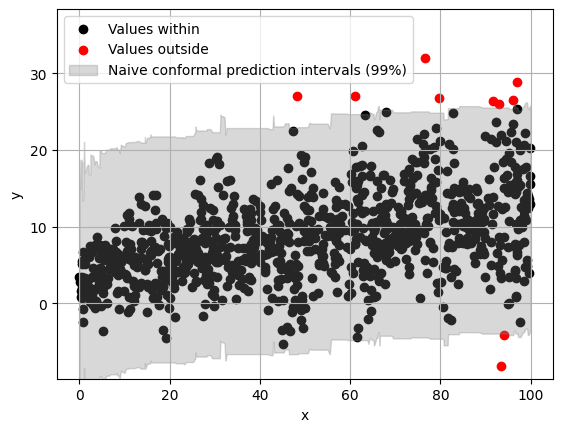
Figure 6: Naive conformal PIs for $\alpha=0.01$.

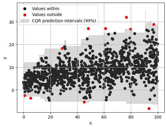
Figure 7: CQR PIs for $\alpha=0.01$.

Figure 8: *

Data generated according to $y=2+\sqrt{x}+\epsilon(x)$, where $\epsilon(x)=\mathcal{N}(0,2+|0.6\sqrt{x}\cos{0,0.2x}|)$ is an heteroscedastic aleatory noise and $x\in[0,100]$. A total of 1000 observations are present in each plot.

2.4 Conformal prediction for time series

The exchangeability assumption of CP, while mild, may not hold for time series data, since the order of observations does matter. To overcome this, several methods suggest rearranging time series in exchangeable blocks that preserve dependency (Chernozhukov et al., 2018; Stankeviciute et al., 2021). However, these blocks still have an inherent order and thus may not be fully exchangeable, hindering the efficacy of CP under these settings.

A more versatile method closely related to Jackknife+-after-bootstrap (Kim et al., 2020) proposed in (Xu & Xie, 2021) is EnbPI. EnbPI utilizes an ensemble learning method called bagging (Breiman, 1996) to mitigate overfitting while generating in-sample non-conformity scores on out-of-bag samples avoiding, therefore, data splitting. The set of non-conformity scores is then updated in batches in the out-of-sample phase, making EnbPI adaptive to distribution shifts. Theoretically, the authors of EnbPI derived tight upper bounds for the absolute difference between the empirical and theoretical error distribution considering a stationary and strongly mixing error process. Empirically, their method ensured the desired coverage over time while ARIMA failed to do so.

Consider a training set $\mathcal{D}_{\text{train}}=\{(\bm{x_{i}},y_{i})\}_{i=1}^{n}$ and an arbitrary regression algorithm $\mathcal{A}$, in practice, EnbPI works as follows:

1. Generate $B$ bootstrap sets from $\mathcal{D}_{\text{train}}$, referred to as $S_{1},..,S_{B}$; 2. Train the regression algorithm on the bootstrap sets to estimate predictors, $\hat{f}^{b}=\mathcal{A}(S_{b}),\quad\forall b\in\{1,..,B\}$; 3. Loop through the training set and aggregate the predictors which did not use the i-th row for training yielding point predictions as $\hat{y}_{i}=\phi(\{\hat{f}^{b}(\bm{x_{i}})\;|\;i\not\in S_{b}\})$, where $\phi$ is a suitable aggregator such as the mean; 4. From the ensemble point predictions, build a set of non-conformity scores ($\bm{\epsilon}$) from absolute errors $\epsilon_{i}=|\hat{y}_{i}-y_{i}|$; 5. Compute $\hat{q}=\text{Quantile}(\bm{\epsilon};1-\alpha)$; 6. For each new out-of-sample set of covariates $\bm{\hat{x}_{n+1}},...,\bm{\hat{x}_{n+H}}$, construct ensemble point predictions for each element of the forecast horizon as $\hat{y}_{n+h}=\phi(\{\hat{f}^{b}(\bm{\hat{x}_{n+h}})\}_{b=1}^{B})$ to then output PIs as $\hat{y}_{n+h}\pm\hat{q}$. After delivering $H$-step ahead PIs and receiving external feedback about the ground truth values $y_{n+1},...,y_{n+H}$, store out-of-sample residuals as $\epsilon_{n+h}=|\hat{y}_{n+h}-y_{n+h}|$ in memory and update $\bm{\epsilon}$ by incorporating these non-conformity scores while discarding the H-th most oldest. Compute $\hat{q}=\text{Quantile}(\bm{\epsilon};1-\alpha)$ again. Repeat this step indefinitely after each $H$-step ahead PIs are produced.

The strength of EnbPI lies in its adaptability, achieved through step 6, where the non-conformity set is transformed into a sliding window of empirical residuals. However, it has a significant drawback when applied to univariate time series forecasting. This issue arises because the in-sample non-conformity scores are computed using actual lag values to generate point predictions whereas, during the out-of-sample phase, each set of covariates $\hat{\bm{x}}_{\bm{n+h}}$ is computed using the recursive strategy formula (as described in (5)). Due to this recursive nature, these values accumulate errors over time, in contrast to the in-sample non-conformity scores which do not reflect this behaviour. Additionally, given that the size of the non-conformity set $(\approx n)$ is usually much larger than the forecast horizon $(H)$, it may take a considerable amount of time before all in-sample non-conformity scores can be discarded. This may result in significant differences between the desired nominal coverage and the observed coverage through a long period a time, despite converging to the specified coverage.

Another drawback of the EnbPI method is its constant PIs width within each batch. However, by utilizing the CQR approach, it is feasible to overcome this limitation. This results in the well-known EnbCQR (Jensen et al., 2022).

2.5 Adaptive conformal inference

ACI (Gibbs & Candes, 2021) is a method designed to extend CP to volatile non-exchangeable settings. The approach involves initializing $\alpha_{1}$ as $\alpha$ and sequentially updating a time-varying $\alpha_{t}$ on received feedback via the following equation

$$\alpha_{t+1}=\alpha_{t}+\gamma(\alpha-\mathbbm{1}\{y_{t}\not\in\hat{C}^{(t)}_{1-\alpha_{t}}(\bm{x_{t}})\}),$$ (13)

where $\gamma$ is a learning rate that controls the method’s adaptation speed to distribution shifts. Note that if the true value is outside the PI, we update the PI width by increasing $\alpha$ using the recursion $\alpha_{t+1}=\alpha_{t}+\gamma(\alpha-1)$. This results in a wider PI for the next iteration, as $\alpha_{t+1}<\alpha_{t}$. On the other hand, if the true value is within the PI, we reduce the width of the PI by increasing $\alpha$, since $\alpha_{t+1}=\alpha_{t}+\gamma\alpha>\alpha_{t}$.

Theoretically, the authors of ACI have demonstrated that for a non-decreasing quantile function, the following inequality holds

$$\left|\frac{1}{n}\sum_{t=1}^{n}\mathbbm{1}\{y_{t}\not\in\hat{C}^{(t)}_{1-\alpha_{t}}(\bm{x_{t}})\}-\alpha\right|\leq\frac{\max\{\alpha_{1},1-\alpha_{1}\}+\gamma}{n\gamma},$$ (14)

which implies that $\lim_{n\rightarrow\infty}\frac{1}{n}\sum_{t=1}^{n}\mathbbm{1}\{y_{t}\not\in\hat{C}^{(t)}_{1-\alpha_{t}}(\bm{x_{t}})\}=\alpha$, demonstrating the method’s asymptotic consistency.

However, in practice, ACI has several bottlenecks. First, nothing prevents $\alpha_{t}<0$, which leads to an infinite PI, despite being highly unlikely to occur in practice, especially if $\gamma$ is small. Second, the learning rate $\gamma$, which is passed as a hyperparameter has strong impact on the method’s efficiency. Lastly, given that the non-conformity set remains unchanged, updating the miscoverage rate $\alpha$ alone may not be sufficient to handle substantial distribution shifts.

Taking into account the last bottleneck of ACI, we have decided to integrate it with a sliding window of empirical residuals in our proposal to further improve adaptability.

3 AEnbMIMOCQR

We now introduce AEnbMIMOCQR, a method that closely follows the structure of EnbPI but offers several additional advantages. Firstly, AEnbMIMOCQR employs the MIMO strategy that always uses actual values as input, avoiding any mismatch between in-sample and out-of-sample non-conformity scores. Secondly, it handles heteroscedasticity by targeting conditional quantiles via a multi-output version of CQR. Thirdly, for situations where $n>>H$ an optional sampling of the non-conformity set without replacement before entering the out-of-sample phase is provided in order to decrease its size and thus improve adaptability. Finally, AEnbMIMOCQR leverages ACI along with a sliding window of non-conformity scores, allowing it to quickly adapt to distribution shifts.

The complete pseudocode of AEnbMIMOCQR is presented in Algorithm (1). The first part of the algorithm focuses on the in-sample phase (lines 1-12), while the second part (lines 17-26) is dedicated to the out-of-sample phase. We also assume that $n_{\text{test}}\equiv 0\mod H$ for simplicity’s sake. To simplify the notation, we have used pairs of vectors $(\bm{x_{i}},\bm{y_{i}})$, where $\bm{x_{i}}$ is the left-hand side and $\bm{y_{i}}$ the right-hand side of line $i$ as in (6).

In terms of coverage, AEnbMIMOCQR PIs are asymptotic valid along the forecast horizon, in the sense of (15).

$$\lim_{n\rightarrow\infty}\frac{1}{n}\sum_{t=1}^{n}\mathbbm{1}\{y_{t,h}\in[\hat{y}_{t,h}^{L},\hat{y}_{t,h}^{U}]\}=1-\alpha,\quad\forall h\in\{1,2...,H\}$$ (15)

Specifically, in the in-sample phase, out-of-bag non-conformity scores are computed for each step ahead from the ensemble multi-output QR models following the non-conformity score function presented in (11) as

$$\epsilon_{t,h}^{\phi}=\max\{\hat{y}_{t,h}^{L}-y_{t,h},y_{t,h}-\hat{y}_{t,h}^{U}\},\quad\forall h\in\{1,...,H\}.$$ (16)

Afterwards, we provide multi-step ahead PIs as

$$[\hat{y}_{t,h}^{L}-\hat{q}^{(h)},\hat{y}_{t,h}^{U}+\hat{q}^{(h)}],\quad\forall h\in\{1,...,H\},$$ (17)

where $\hat{q}^{(h)}$ is the h-step ahead QR’s CP correction.

Similarly to EnbPI, in the out-of-sample phase, the non-conformity set is updated with new non-conformity scores after generating $H$-step ahead PIs. In addition, ACI is utilized initializing $\alpha_{h}$ as $\alpha$, where $\alpha_{h}$ is the miscoverage rate for the $h$-step ahead. In line 16 of Algorithm (1), the symbol $\bm{\epsilon_{h}}^{{}^{\prime}}$ refers to the non-conformity set obtained from $\bm{\epsilon_{h}}$ after sampling $T$ scores without replacement. The user specifies the dimension of $\bm{\epsilon_{h}}^{{}^{\prime}}$ as $T$, which is chosen to be much smaller than the original dimension $(\approx n)$ of $\bm{\epsilon_{h}}$. This reduction in dimension is intended to improve the adaptability of the algorithm.

For instance, if $\bm{\epsilon_{h}}$ has a dimension of $10,000$ and $H=10$ for each $h$-step ahead, the update of the empirical quantiles after producing the first $H$-step ahead PIs and updating the non-conformity set will be negligible. This is because the dimension of the non-conformity set is much larger than $H$. However, by specifying $T=100$ and using the sampled version $\bm{\epsilon_{h}}^{{}^{\prime}}$ instead of $\bm{\epsilon_{h}}$, the effect on the empirical quantiles will be more significant since the dimension is now much smaller and closer to $H$. Undoubtedly, information loss is inevitable in this process, however it is worth employing in practice considering the gains in adaptability.

Overall, AEnbMIMOCQR is expected to comply with the criteria initially presented in Section 1, implying it should empirically deliver the desired nominal coverage along the forecast horizon even on the most adverse volatile settings.

Algorithm 1 AEnbMIMOCQR algorithm

.

1:A training set $\{(\bm{x_{i}},\bm{y_{i}})\}_{i=1}^{n}$, miscoverage rate $\alpha$, a multi-output QR algorithm $\mathcal{A}_{\tau}$, an aggregation function $\phi$, number of bootstrap models $B$, the forecast horizon $H$, $T$ observations to sample without replacement, a test set $\{(\bm{x_{t}},\bm{y_{t}})\}_{t=n+1}^{n+n_{\text{test}}}$ with $\bm{y_{t}}$ revealed only at timestep $t+H$.

2:PIs for $\bm{x_{n+1}},\bm{x_{n+1+H}},...,\bm{x_{n+n_{\text{test}}}}$.

3:for $b\leftarrow 1,...,B$ do

4:     Sample an index set $S_{b}=(i_{1},...,i_{T})$ from indices (1,…,$n$)

5:     Train $\hat{F}_{\alpha/2}^{b}\leftarrow\mathcal{A}_{\alpha/2}(\{(\bm{x_{i}},\bm{y_{i}})\;|\;i\in S_{b}\})$

6:     Train $\hat{F}_{1-\alpha/2}^{b}\leftarrow\mathcal{A}_{1-\alpha/2}(\{(\bm{x_{i}},\bm{y_{i}})\;|\;i\in S_{b}\})$

7:end for

8:$\bm{\epsilon}_{h}\leftarrow\{\},\quad\forall h\in\{1,...,H\}$

9:for $i\leftarrow 1,...,n$ do

10:     $[\hat{y}_{i,1}^{L},...,\hat{y}_{i,H}^{L}]\leftarrow\phi(\{(\hat{F}_{\alpha/2}^{b}(\bm{x_{i}})|\;i\not\in S_{b}\})$

11:     $[\hat{y}_{i,1}^{U},...,\hat{y}_{i,H}^{U}]\leftarrow\phi(\{(\hat{F}_{1-\alpha/2}^{b}(\bm{x_{i}})|\;i\not\in S_{b}\})$

12:     $\epsilon_{i,h}^{\phi}\leftarrow\max{\{\hat{y}_{i,h}^{L}-y_{i,h},y_{i,h}-\hat{y}_{i,h}^{U}\}},\quad\forall h\in\{1,...,H\}$

13:     $\bm{\epsilon}_{h}\leftarrow\bm{\epsilon}_{h}\cup\{\epsilon_{i,h}^{\phi}\},\quad\forall h\in\{1,...,H\}$

14:end for

15:$\gamma\leftarrow 1/\max\{T,|\bm{\epsilon_{1}}|\}$

16:$\alpha_{h}\leftarrow\alpha,\quad\forall h\in\{1,...,H\}$

17:$\hat{q}^{(h)}\leftarrow\text{Quantile}(\bm{\epsilon_{h}};1-\alpha_{h}),\quad\forall h\in\{1,...,H\}$

18:$\bm{\epsilon_{h}}^{{}^{\prime}}\leftarrow\text{Sample}(T,\bm{\epsilon_{h}}),\quad\forall h\in\{1,...,H\}$

19:for $t\leftarrow n+1,n+1+H,...,n+n_{\text{test}}$ do

20:     $[\hat{y}_{t,1}^{L},...,\hat{y}_{t,H}^{L}]\leftarrow\phi(\{(\hat{F}_{\alpha/2}^{b}(\bm{x_{t}})\}_{b=1}^{B})$

21:     $[\hat{y}_{t,1}^{U},...,\hat{y}_{t,H}^{U}]\leftarrow\phi(\{(\hat{F}_{1-\alpha/2}^{b}(\bm{x_{t}})\}_{b=1}^{B})$

22:     Return $\hat{C}_{1-\alpha_{h}}^{(t)}(\bm{x_{t}})\leftarrow[\hat{y}_{t,h}^{L}-\hat{q}^{(h)},\hat{y}_{t,h}^{U}+\hat{q}^{(h)}],\quad\forall h\in\{1,...,H\}$

23:     $\epsilon_{h}^{(*)}\leftarrow\max{\{(\hat{y}_{t,h}^{L}-\hat{q}^{(h)})-y_{t,h},y_{t,h}-(\hat{y}_{t,h}^{U}+\hat{q}^{(h)})\}},\quad\forall h\in\{1,...,H\}$

24:     $\bm{\epsilon}_{h}^{{}^{\prime}}\leftarrow(\bm{\epsilon}_{h}^{{}^{\prime}}-\{\epsilon_{1,h}\})\cup\{\epsilon_{h}^{(*)}\},\quad\forall h\in\{1,...,H\}$ and reset index of $\bm{\epsilon}_{h}$

25:     $\alpha_{h}\leftarrow\alpha_{h}+\gamma(\alpha-\mathbbm{1}\{y_{t,h}\not\in\hat{C}_{1-\alpha}^{(t)}(\bm{x_{t}})\}),\quad\forall h\in\{1,...,H\}$

26:     $\alpha_{h}\leftarrow\max\{0,\min\{\alpha_{h},1\}\},\quad\forall h\in\{1,...,H\}$

27:     Update $\hat{q}^{(h)}\leftarrow\text{Quantile}(\bm{\epsilon_{h}^{{}^{\prime}}};1-\alpha_{h}),\quad\forall h\in\{1,...,H\}$

28:end for

3.1 AEnbMIMOCQR for multivariate time series

Thus far, this article has solely tackled conformal univariate time series forecasting; however, in many applications, the covariates are lagged multidimensional features that intend to estimate a $H$-step ahead multidimensional target, therefore the traning set $\mathcal{D}_{\text{train}}=\{(\bm{X_{i}},\bm{Y_{i}})\}_{i=1}^{n}$ is used to estimate the desired function $F:\mathbb{R}^{p\times F_{1}}\rightarrow\mathbb{R}^{H\times F_{2}}$, where $F_{1}\geq F_{2}$ are the number of input and output features, respectively. AEnbMIMOCQR can handle this setting by training a suitable ML model (e.g. (Hochreiter & Schmidhuber, 1997)) set to minimize the pinball loss and by also modifying Algorithm (1) accordingly, so that we have $H\times F_{2}$ non-conformity sets, $\alpha$s, and $\hat{q}$s, one per each feature and horizon.

In the interest of space, Algorithm (1) will not be reproduced to contemplate this case since the generalization is straightforward from here.

4 Experimental design

The goal of the experimental part is to compare the PIs generated by the AEnbMIMOCQR method against those generated by four other methods: EnbPI, EnbCQR, ARIMA, and MIMOCQR, which is a simplified version of AEnbMIMOCQR that does not adapt to distribution shifts and does not use bagging (Breiman, 1996). Although the quality of the PIs generated by the conformal methods depends on the underlying regression algorithm, finding the best architecture is outside the scope of this study. Instead, the same architecture is employed for all methods, enabling a fair comparison of their relative performance. Table (1) displays the global parameters used in the experiment.

Parameter	value
$\alpha$	0.1
Number of lags (p)	40
Forecast horizon (H)	30

Table 1: Global parameters used throughout the experiment.

4.1 Datasets

To evaluate the efficacy of the methods, two experiments were conducted. The first experiment employed a real-world dataset, while the second experiment was conducted using a synthetic dataset to provide a more controlled setting since the aleatory noise distribution is known.

4.1.1 Real-world

The real-world dataset is the NN5 forecasting competition dataset (NN, 5). This dataset comprises 111 time series, with each time series consisting of 791 daily cash machine withdrawals recorded at a specific location in England. This dataset is a suitable choice for this analysis since, as shown in Table (2), the Augmented Dickey-Fuller test (Dickey & Fuller, 1979, 1981) indicates that a reasonable amount of time series are non-stationary for a maxlag of 40.

Significance level	#series
0.1	92
0.05	84
0.01	67

Table 2: Number of stationary time series for different significance levels of the Augmented Dickey-Fuller test.

4.1.2 Synthetic

In order to create a controlled experimental environment, data is generated using (18), where $\{Y_{i}\}_{i=1}^{40}\sim\text{U}(0,1)$ and $c_{t}=0.1+t/1000$. This allows for a rigorous comparison between methods, as we have direct access to the oracle PIs. Additionally, since the data-generating process is dynamic it enables us to assess how different methods adapt to distribution shifts.

$$Y_{t}=\mathcal{N}\left(\log\left(\sum_{i=1}^{40}Y_{t-i}^{2}\right),c_{t}\log\left(\sum_{i=1}^{40}Y_{t-i}^{2}\right)\right),\quad t=41,...,1041.$$ (18)

4.2 Experimental setup

In this experiment, a multilayer perceptron (Noriega, 2005) regression algorithm with two hidden layers and 64 neurons in each layer was utilized. The models were estimated using ADAM (Kingma & Ba, 2014) as a optimizer for 1000 epochs. The architecture of the regression algorithm differed for AEnbMIMOCQR and MIMOCQR, both having an $H$-dimensional output layer, while EnbCQR and EnbPI, had a $1$-dimensional output layer. Additionally, while EnbPI was set to minimize the mean squared error, the other competitive methods were set to minimize the pinball loss at the quantiles of interest. The mean function was used to aggregate 10 bootstrap models ($B=10\text{ and }\phi=\text{'mean'}$) for all models. $T$ was set to 100 on AEnbMIMOCQR for both datasets. The number of testing observations was set to 390, therefore $n_{\text{test}}=390$, leaving the remainder for training. The experiment was conducted using the Python programming language along with the tensorflow (Abadi et al., 2015) and pmdarima (Smith et al., 2017) libraries.

4.3 Evaluation performance measures

The quality of the delivered PIs in the real-world dataset was evaluated using two performance measures: prediction interval coverage probability (PICP), which assesses the calibration, and prediction interval normalized average width (PINAW), which measures the sharpness. The PICP performance measure can also be found in (Shepero et al., 2018; Jensen et al., 2022) and is defined in (19), while the PINAW performance measure can be found in (Kavousi-Fard, 2016; Jensen et al., 2022) and is defined in (20). Note that different performance measure could be used such as the scalled pinball loss (Makridakis et al., 2022b) or Winkler score (Winkler, 1972). However, we prefer to report sharpness and calibration separately since for critical applications, ensuring the desired nominal coverage is the primary concern over shorter PIs. Moreover, performance measures such as the Winkler score are not adequate for evaluating PIs that aim to capture heteroscedasticity noises.

In the synthetic dataset, a third performance measure inspired by insersection over union (IOU) was employed. This performance measure penalizes PIs that deviate from the oracle PIs, whether they are overly conservative or under conservative. We name it mean intersection over union (MIOU) since it is the average IOU over the test set. The formula is presented in (21).

$$\text{PICP}=\frac{1}{n_{\text{test}}}\sum_{t=1}^{n_{\text{test}}}\mathbbm{1}\left\{y_{t}\in[\hat{y}^{L}_{t},\hat{y}^{U}_{t}]\right\},$$ (19)

$$\text{PINAW}=\frac{1}{n_{\text{test}}(y_{\text{max}}-y_{\text{min}})}\sum_{t=1}^{n_{\text{test}}}(\hat{y}^{U}_{t}-\hat{y}^{L}_{t}),$$ (20)

$$\text{MIOU}=\frac{1}{n_{\text{test}}}\sum_{t=1}^{n_{\text{test}}}\frac{|[\hat{y}^{L}_{t},\hat{y}^{U}_{t}]\cap[y^{L}_{t},y^{U}_{t}]|}{|[\hat{y}^{L}_{t},\hat{y}^{U}_{t}]\cup[y^{L}_{t},y^{U}_{t}]|}=\frac{1}{n_{\text{test}}}\sum_{t=1}^{n_{\text{test}}}\frac{|[\max\{\hat{y}^{L}_{t},y^{L}_{t}\},\min\{\hat{y}^{U}_{t},y^{U}_{t}\}]|}{|[\min\{\hat{y}^{L}_{t},y^{L}_{t}\},\max\{\hat{y}^{U}_{t},y^{U}_{t}]|}.$$ (21)

5 Results and analysis

5.1 Real-world dataset

The results of all methods with the parameters specified in the last section are summarized in Table (3). Figure 9 shows the PICP boxplot scores for all methods. Since we are comparing 111 series and the chosen performance measures are scale-independent, we have calculated the average values across all series, according to (22) and (23).

Upon inspecting Table (3) results, it becomes evident that AEnbMIMOCQR outperforms its competitors in terms of observed coverage, as indicated by its $\text{PICP}^{*}$ score, which is closer to the desired nominal coverage of 0.9. Furthermore, its PIs width is lower than that of EnbPI and EnbCQR, most likely due to not accumulating errors over the forecast horizon. ARIMA method appears to be the furthest from achieving the desired nominal coverage. Although it produces wide PIs according to its $\text{PINAW}^{*}$, they seem to be mislocated. Given that the data-generating process is unknown, we cannot pinpoint the specific reasons for this issue. However, it is likely due to one or more violations of the many rigid assumptions underlying the method. As for the adaptive components that integrate AEnbMIMOCQR such as ACI and a sliding window of empirical residuals, they play a crucial role in achieving a 0.078 higher $\text{PICP}^{*}$ score by comparing it to MIMOCQR.

Moreover, Figure 9 reveals that the spread of AEnbMIMOCQR is lower, which is expected based on the algorithm formulation. While AEnbMIMOCQR seeks to ensure exact nominal coverage and updates the $\alpha$ when the algorithm is either overcovering or undercovering, its competitors do not, justifying the shorter spread.

$$\text{PICP}^{*}=\frac{1}{111}\sum_{i=1}^{111}\text{PICP}_{i}$$ (22)

$$\text{PINAW}^{*}=\frac{1}{111}\sum_{i=1}^{111}\text{PINAW}_{i}$$ (23)

Method	$\textbf{PICP}^{*}$	$\textbf{PINAW}^{*}$
AEnbMIMOCQR	0.882	0.357
MIMOCQR	0.804	0.283
EnbPI	0.862	0.493
EnbCQR	0.866	0.370
ARIMA	0.723	0.403

Table 3: Relative performance measures obtained on the real-world dataset.

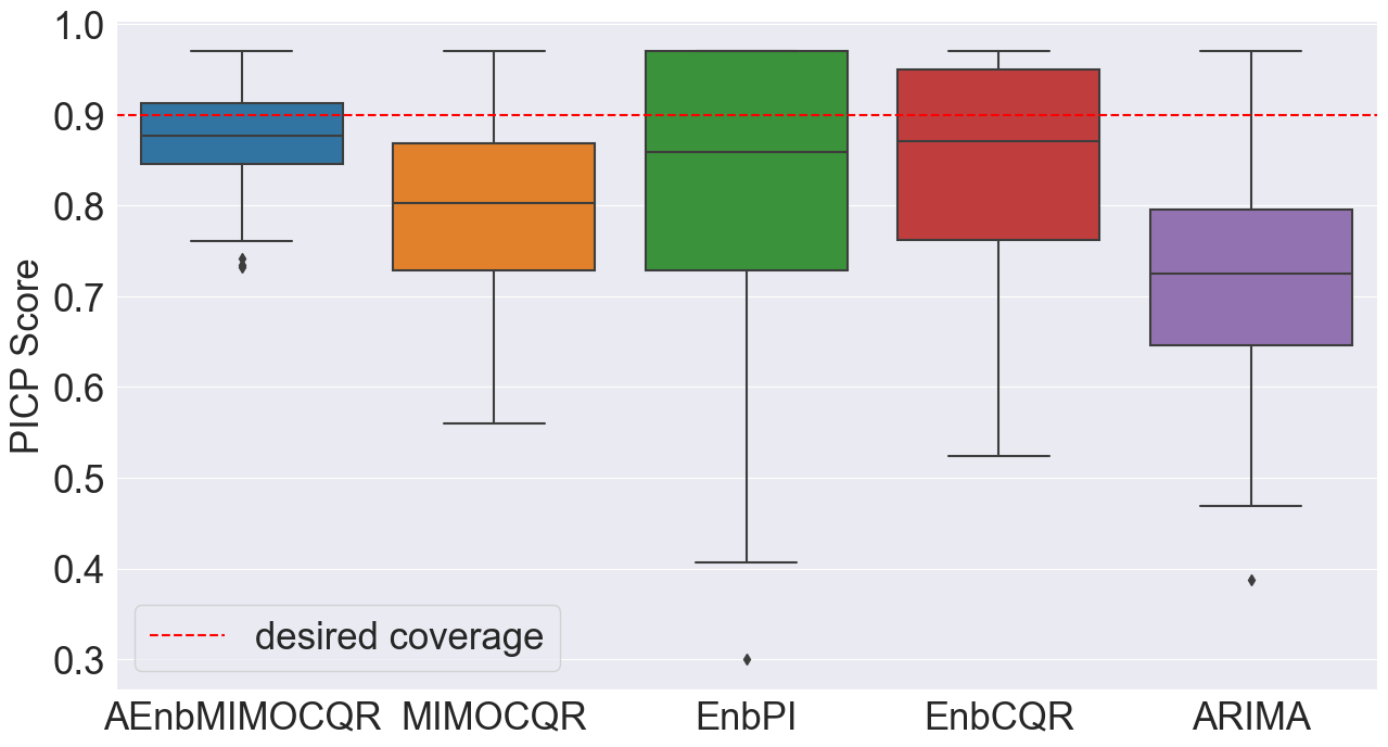
Figure 9: PICP score boxplot of all methods computed on the NN5 daataset.

5.2 Synthetic dataset

The experiments conducted on the synthetic dataset have shown results that are consistent with those obtained on the real-world dataset. However, this additional experiment is key since relying solely on measures such as PICP and PINAW may not be sufficient if the goal is to assess conditional nominal coverage. In such cases, it is essential to consider other performance measures, such as MIOU, which can effectively take into account the heteroscedasticity of the dataset. Therefore, based on the evidence shown in Table (4), AEnbMIMOCQR gets closer in achieving conditional nominal coverage, where a MIOU score of 1 signifies perfect conditional nominal coverage.

Method	MIOU
AEnbMIMOCQR	0.843
MIMOCQR	0.784
EnbPI	0.752
EnbCQR	0.796
ARIMA	0.622

Table 4: MIOU scores on the synthetic dataset.

6 Discussion and conclusions

In this paper, we proposed a novel algorithm called AEnbMIMOCQR that extends CP for multi-step ahead regression tasks without relying on exchangeability assumptions. Although previous work, such as EnbPI and EnbCQR, has explored the extension of CP to non-exchangeable data settings, our algorithm demonstrated faster adaptation to distribution shifts. Specifically, we observed more consistent observed coverage levels when compared to competing methods, as well as shorter and input-varying PIs. Moreover, using ACI, bagging, and a sliding window of empirical non-conformity scores revealed key as, contrarily to the simplified version, MIMOCQR, the observed coverage closely aligns with the desired nominal coverage. These results highlight the potential benefits of using AEnbMIMOCQR in real-world applications where distribution shifts and heteroscedasticity may occur, enhancing decision-making in critical applications.

Regardless of whether the data is heteroscedastic or not, we concur with the recommendation of Jensen et al. (2022) to always use heteroscedastic methods such as EnbCQR and AEnbMIMOCQR. Even in cases where the data is homoscedastic, the PIs produced by EnbCQR will be similar to those of EnbPI.

Topics worth exploring in the future are: (i) devise a clever mechanism on the choice of $\gamma$ in ACI, as it an important impact on the method’s adaptation speed; (ii) comparing our approach against different forecasting strategies for multi-step ahead forecasting presented in the literature; (iii) instead of discarding the oldest non-conformity scores, discard according to a a better criteria (e.g., discard those that are less likely to belong the current data distribution); (iv) utilizing asymmetric and heteroscedasticity aware non-conformity measures (Kivaranovic et al., 2020); and (v) employing ACI in conjunction with EnbCQR or EnbPI.

To conclude, AEnbMIMOCQR is a step further on extending CP for multi-step ahead forecasting in time series and may certainly encounter several applications in real-world sectors including, but not limited to, energy, finance, and retail.

CRediT authorship contribution statement

Martim Sousa: Writing - original draft, Writing - review & editing, Problem conceptualization, Methodology, Algorithm development, Investigation, Programming, Data analysis, Data curation. Ana Tomé: Writing - review & editing, Supervision, Validation. José Moreira: Writing - review & editing, Supervision, Validation, Funding acquisition.

Declaration of Competing Interest

The authors declare that they have no known competing financial interests or personal relationships that could have appeared to influence the work reported in this paper.

Appendix A Proofs

Definition 3 (Exchangeability).

A sequence of random variables $Z_{1},Z_{2},...,Z_{n}\in\mathcal{Z}$ are exchangeable if and only if for any permutation $\pi:\{1,2,...,n\}\rightarrow\{1,2,...,n\}$, we have

$$\mathbb{P}\{Z_{1},Z_{2},...,Z_{n}\}=\mathbb{P}\{Z_{\pi(1)},Z_{\pi(2)},...,Z_{\pi(n)}\}$$ (24)

Lemma 1.

Let $Z_{1},...,Z_{n}\in\mathcal{Z}$ be exchangeable random variables with no ties almost surely, then their ranks are uniformly distributed on {1,…,n}.

Proof.

Let $R_{i}=\text{Rank}(Z_{i})$. Since $Z_{1},\ldots,Z_{n}$ are exchangeable, there are $n!$ equally probable permutations of the variables. Furthermore, because $Z_{1},\ldots,Z_{n}$ have no ties almost surely, we have $\mathbb{P}(R_{i}\neq R_{j})=1$ for all $i\neq j\in\{1,\ldots,n\}$.

For any $i\in\{1,...,n\}$, if we fix $R_{i}$ on rank $j\in\{1,...,n\}$, then there are (n-1)! possible permutations among the other n-1 random variables. Hence, $\mathbb{P}(R_{i}=j)=\frac{(n-1)!}{n!}=\frac{1}{n}$ and thus

$$\mathbb{P}(R_{i}=1)=\mathbb{P}(R_{i}=2)=...=\mathbb{P}(R_{i}=n)=\frac{1}{n},\quad\forall i\in\{1,...,n\}.$$

This shows that the ranks of the variables are uniformly distributed on ${1,\ldots,n}$. ∎

Theorem 2 (Marginal coverage guarantee).

Let $(\bm{X_{1}},Y_{1}),...,(\bm{X_{n}},Y_{n})$ be exchangeable random vectors with no ties almost surely drawn from a distribution P, additionally if for a new pair $(\bm{X_{n+1}},Y_{n+1})$, $(\bm{X_{1}},Y_{1}),...,(\bm{X_{n+1}},Y_{n+1})$ are still exchangeable, then by constructing $C_{1-\alpha}(\bm{X_{n+1}})$ using CP, the following inequality holds for any non-conformity score function $s:\mathcal{X}\times\mathcal{Y}\rightarrow\mathcal{A}\subseteq\mathbb{R}$ and any $\alpha\in(\frac{1}{n+1},1)$

$$1-\alpha\leq\mathbb{P}\{Y_{n+1}\in C_{1-\alpha}(\bm{X_{n+1}})\}\leq 1-\alpha+\frac{1}{n+1}.$$ (25)

Proof.

Since $\bm{Z_{1}}=(\bm{X_{1}},Y_{1}),...,\bm{Z_{n}}=(\bm{X_{n}},Y_{n})$ are exchangeable random vectors with no ties almost surely, the corresponding non-conformity scores $\bm{\epsilon}=\{(\epsilon_{i}:=s(\bm{Z_{i}}))\}_{i=1}^{n}$ are also exchangeable (by Theorem 3 of (Kuchibhotla, 2020)) with no ties almost surely. Since the non-conformity scores $\epsilon_{1},...,\epsilon_{n},\epsilon_{n+1}$ are exchangeable, their ranks are uniformly distributed by Lemma (1). Therefore, $\text{Rank}(\epsilon_{n+1})\sim\mathcal{U}\{1,n+1\}$. That is,

$$\mathbb{P}\{\epsilon_{n+1}\leq\epsilon_{(k)}\}=\mathbb{P}\{\text{Rank}(\epsilon_{n+1})\leq k\}=\frac{k}{n+1},\quad\forall k\in\{1,...,n+1\}.$$

By definition, since $\hat{q}=\text{Quantile}(\bm{\epsilon};\frac{\lceil(n+1)(1-\alpha)\rceil}{n})=\epsilon_{(\lceil(n+1)(1-\alpha)\rceil)}$, follows that

$$\mathbb{P}\{Y_{n+1}\in C_{1-\alpha}(\bm{X_{n+1})}\}=\mathbb{P}\{y\in\mathcal{Y}:s(\bm{X_{n+1}},y)\leq\hat{q}\}=\mathbb{P}\{\epsilon_{n+1}\leq\epsilon_{(\lceil(n+1)(1-\alpha)\rceil)}\}=\frac{\lceil(n+1)(1-\alpha)\rceil}{n+1}.$$

It is easy to note that $1-\alpha\leq\frac{\lceil(n+1)(1-\alpha)\rceil}{n+1}\leq\frac{(n+1)(1-\alpha)+1}{n+1}=1-\alpha+\frac{1}{n+1}$. ∎

Appendix B Algorithms

Algorithm 2 EnbPI algorithm adapted to recursive $H$-step ahead PIs. (Xu & Xie, 2021)

.

1:Training data $\{(\bm{x_{i}},y_{i})\}_{i=1}^{n}$, regression algorithm $\mathcal{A}$, miscoverage rate $\alpha$, aggregation function $\phi$, number of bootstrap models $B$, the forecast horizon $H$, and test data $\{(\bm{x_{t}},y_{t})\}_{t=n+1}^{n+n_{\text{test}}}$, with $y_{t}$ revealed only after $H$ timesteps.

2:PIs: $\{\hat{C}_{1-\alpha}^{(t)}(\bm{x_{t}})\}_{t=n+1}^{n+n_{\text{test}}}$

3:for b=1,…,B do

4:     Sample an index set $S_{b}=(i_{1},...,i_{T})$ from indices (1,…,n)

5:     Train $\hat{f}^{b}\leftarrow\mathcal{A}(\{\bm{x_{i}},y_{i})\;|\;i\in S_{b}\})$

6:end for

7:$\bm{\epsilon}\leftarrow\{\}$

8:for $i\leftarrow 1,...,n$ do

9:     $\hat{y}_{i}\leftarrow\phi(\{\hat{f}^{b}(\bm{x_{i}})\;|\;i\not\in S_{b}\})$

10:     $\epsilon_{i}^{\phi}\leftarrow|\hat{y}_{i}-y_{i}|$

11:     $\bm{\epsilon}\leftarrow\bm{\epsilon}\cup\{\ \epsilon_{i}^{\phi}\}$

12:end for

13:$\hat{q}\leftarrow\text{Quantile}\left(\bm{\epsilon};1-\alpha\right)$

14:for $t\leftarrow n+1,...,n+n_{\text{test}}$ do

15:     Compute $\hat{\bm{x_{t}}}$ using the recursive strategy formula (see (5)) for $h=t-T\mod H$

16:     $\hat{y}_{t}\leftarrow\phi(\{\hat{f}^{b}(\bm{x_{t}})\}_{b=1}^{B})$

17:     Return $\hat{C}_{1-\alpha}^{(t)}(\bm{x_{t}})\leftarrow[\hat{y}_{t}-\hat{q},\hat{y}_{t}+\hat{q}]$

18:     if $t-T\equiv 0\mod H$ then

19:         for $j\leftarrow t-H,...,t-1$ do

20:              $\epsilon_{j}^{\phi}\leftarrow|\hat{y}_{j}-y_{j}|$

21:              $\bm{\epsilon}\leftarrow(\bm{\epsilon}-\{\epsilon_{1}^{\phi}\})\cup\{\epsilon_{j}^{\phi}\}$ and reset index of $\bm{\epsilon}$

22:         end for

23:         Update $\hat{q}\leftarrow\text{Quantile}\left(\bm{\epsilon};1-\alpha\right)$

24:     end if

25:end for

Algorithm 3 EnbCQR algorithm adapted to recursive $H$-step ahead PIs. (Jensen et al., 2022)

.

1:Training data $\{(\bm{x_{i}},y_{i})\}_{i=1}^{n}$, regression single-output QR algorithm $\mathcal{A}_{\tau}$, miscoverage rate $\alpha$, aggregation function $\phi$, number of bootstrap models $B$, the forecast horizon $H$, and test data $\{(\bm{x_{t}},y_{t})\}_{t=n+1}^{n+n_{\text{test}}}$, with $y_{t}$ revealed only after $H$ timesteps.

2:PIs: $\{\hat{C}_{1-\alpha}^{(t)}(\bm{x_{t}})\}_{t=n+1}^{n+n_{\text{test}}}$

3:for b=1,…,B do

4:     Sample an index set $S_{b}=(i_{1},...,i_{T})$ from indices (1,…,n)

5:     Train $\hat{f}_{\alpha/2}^{b}\leftarrow\mathcal{A}_{\alpha/2}(\{\bm{x_{i}},y_{i})\;|\;i\in S_{b}\})$

6:     Train $\hat{f}_{0.5}^{b}\leftarrow\mathcal{A}_{0.5}(\{\bm{x_{i}},y_{i})\;|\;i\in S_{b}\})$

7:     Train $\hat{f}_{1-\alpha/2}^{b}\leftarrow\mathcal{A}_{1-\alpha/2}(\{\bm{x_{i}},y_{i})\;|\;i\in S_{b}\})$

8:end for

9:$\bm{\epsilon}\leftarrow\{\}$

10:for $i\leftarrow 1,...,n$ do

11:     $\hat{y}_{i}^{L}\leftarrow\phi(\{\hat{f}^{b}_{\alpha/2}(\bm{x_{i}})\;|\;i\not\in S_{b}\})$

12:     $\hat{y}_{i}^{U}\leftarrow\phi(\{\hat{f}^{b}_{1-\alpha/2}(\bm{x_{i}})\;|\;i\not\in S_{b}\})$

13:     $\epsilon_{i}^{\phi}\leftarrow\max\{\hat{y}_{i}^{L}-y_{i},y_{i}-\hat{y}_{i}^{U}\}$

14:     $\bm{\epsilon}\leftarrow\bm{\epsilon}\cup\{\ \epsilon_{i}^{\phi}\}$

15:end for

16:$\hat{q}\leftarrow\text{Quantile}\left(\bm{\epsilon};1-\alpha\right)$

17:for $t\leftarrow n+1,...,n+n_{\text{test}}$ do

18:     Compute $\hat{\bm{x_{t}}}$ using $\{\hat{f}^{b}_{0.5}\}_{b=1}^{B}$ and the recursive strategy formula (see (5)) for $h=t-T\mod H$

19:     $\hat{y}_{t}^{L}\leftarrow\phi(\{\hat{f}^{b}_{\alpha/2}(\hat{\bm{x_{t}}})\}_{b=1}^{B})$

20:     $\hat{y}_{t}^{U}\leftarrow\phi(\{\hat{f}^{b}_{1-\alpha/2}(\hat{\bm{x_{t}}})\}_{b=1}^{B})$

21:     Return $\hat{C}_{1-\alpha}^{(t)}(\bm{x_{t}})\leftarrow[\hat{y}_{t}^{L}-\hat{q},\hat{y}_{t}^{U}+\hat{q}]$

22:     if $t-T\equiv 0\mod H$ then

23:         for $j\leftarrow t-H,...,t-1$ do

24:              $\epsilon_{j}^{\phi}\leftarrow\max\{\hat{y}_{i}^{L}-y_{i},y_{i}-\hat{y}_{i}^{U}\}$

25:              $\bm{\epsilon}\leftarrow(\bm{\epsilon}-\{\epsilon_{1}^{\phi}\})\cup\{\epsilon_{j}^{\phi}\}$ and reset index of $\bm{\epsilon}$

26:         end for

27:         Update $\hat{q}\leftarrow\text{Quantile}\left(\bm{\epsilon};1-\alpha\right)$

28:     end if

29:end for

Algorithm 4 MIMOCQR algorithm to obtain $H$-step ahead PIs

.

1:A training set $\{(\bm{x_{i}},\bm{y_{i}})\}_{i=1}^{n}$, a calibration set $\{(\bm{x_{i}},\bm{y_{i}})\}_{i=n+1}^{n+n_{\text{cal}}}$, miscoverage rate $\alpha$, a multi-output QR algorithm $\mathcal{A}_{\tau}$, the forecast horizon $H$, and a test set $\{(\bm{x_{t}},\bm{y_{t}})\}_{t=n+n_{\text{cal}}+1}^{n+n_{\text{cal}}+n_{\text{test}}}$ with $\bm{y_{t}}$ revealed only at timestep $t+H$.

2:PIs $\{\hat{C}_{1-\alpha}^{(t)}(\bm{x_{t}})\}_{t=n+1}^{n+n_{\text{test}}}$

3:Train $\hat{F}_{\alpha/2}\leftarrow\mathcal{A}_{\alpha/2}(\{(\bm{x_{i}},\bm{y_{i}})\;|\;i\in\{1,...,n\}\})$

4:Train $\hat{F}_{1-\alpha/2}\leftarrow\mathcal{A}_{1-\alpha/2}(\{(\bm{x_{i}},\bm{y_{i}})\;|\;i\in\{1,...,n\}\})$

5:$\bm{\epsilon}_{h}\leftarrow\{\},\quad\forall h\in\{1,...,H\}$

6:for $i\leftarrow n+1,...,n+n_{\text{cal}}$ do

7:     $[\hat{y}_{i,1}^{L},...,\hat{y}_{i,H}^{L}]\leftarrow\hat{F}_{\alpha/2}(\bm{x_{i}})$

8:     $[\hat{y}_{i,1}^{U},...,\hat{y}_{i,H}^{U}]\leftarrow\hat{F}_{1-\alpha/2}(\bm{x_{i}})$

9:     $\epsilon_{i,h}^{\phi}\leftarrow\max{\{\hat{y}_{i,h}^{L}-y_{i,h},y_{i,h}-\hat{y}_{i,h}^{U}\}},\quad\forall h\in\{1,...,H\}$

10:     $\bm{\epsilon}_{h}\leftarrow\bm{\epsilon}_{h}\cup\{\epsilon_{i,h}^{\phi}\},\quad\forall h\in\{1,...,H\}$

11:end for

12:$\hat{q}^{(h)}\leftarrow\text{Quantile}(\bm{\epsilon_{h}};1-\alpha),\quad\forall h\in\{1,...,H\}$

13:for $t\leftarrow n+n_{\text{cal}}+1,n+n_{\text{cal}}+H+1,...,n+n_{\text{cal}}+n_{\text{test}}$ do

14:     $[\hat{y}_{t,1}^{L},...,\hat{y}_{t,H}^{L}]\leftarrow\hat{F}_{\alpha/2}(\bm{x_{t}})$

15:     $[\hat{y}_{t,1}^{U},...,\hat{y}_{t,H}^{U}]\leftarrow\hat{F}_{1-\alpha/2}(\bm{x_{t}})$

16:     Return $\hat{C}_{1-\alpha}^{(t)}(\bm{x_{t}})\leftarrow[\hat{y}_{t,h}^{L}-\hat{q}^{(h)},\hat{y}_{t,h}^{U}+\hat{q}^{(h)}],\quad\forall h\in\{1,...,H\}$

17:end for

References

- NN (5) (). Nn5 forecasting competion dataset. http://www.neural-forecasting-competition.com/NN5/. Accessed: April 7, 2023.
- Abadi et al. (2015) Abadi, M., Agarwal, A., Barham, P., Brevdo, E., Chen, Z., Citro, C., Corrado, G. S., Davis, A., Dean, J., Devin, M., Ghemawat, S., Goodfellow, I., Harp, A., Irving, G., Isard, M., Jia, Y., Jozefowicz, R., Kaiser, L., Kudlur, M., Levenberg, J., Mané, D., Monga, R., Moore, S., Murray, D., Olah, C., Schuster, M., Shlens, J., Steiner, B., Sutskever, I., Talwar, K., Tucker, P., Vanhoucke, V., Vasudevan, V., Viégas, F., Vinyals, O., Warden, P., Wattenberg, M., Wicke, M., Yu, Y., & Zheng, X. (2015). TensorFlow: Large-scale machine learning on heterogeneous systems. URL: https://www.tensorflow.org/ software available from tensorflow.org.
- An & Anh (2015) An, N. H., & Anh, D. T. (2015). Comparison of strategies for multi-step-ahead prediction of time series using neural network. In 2015 International Conference on Advanced Computing and Applications (ACOMP) (pp. 142–149). IEEE.
- Angelopoulos & Bates (2023) Angelopoulos, A. N., & Bates, S. (2023). Conformal prediction: A gentle introduction. Foundations and Trends® in Machine Learning, 16, 494–591. URL: http://dx.doi.org/10.1561/2200000101. doi:10.1561/2200000101.
- Barber et al. (2021) Barber, R. F., Candes, E. J., Ramdas, A., & Tibshirani, R. J. (2021). Predictive inference with the jackknife+, .
- Breiman (1996) Breiman, L. (1996). Bagging predictors. Machine learning, 24, 123–140.
- Brockwell & Davis (2002) Brockwell, P. J., & Davis, R. A. (2002). Introduction to time series and forecasting. Springer.
- Chatfield (2001) Chatfield, C. (2001). Prediction intervals for time-series forecasting. Principles of forecasting: A handbook for researchers and practitioners, (pp. 475–494).
- Chernozhukov et al. (2018) Chernozhukov, V., Wüthrich, K., & Yinchu, Z. (2018). Exact and robust conformal inference methods for predictive machine learning with dependent data. In Conference On learning theory (pp. 732–749). PMLR.
- Cochrane (2005) Cochrane, J. H. (2005). Time series for macroeconomics and finance. Manuscript, University of Chicago, 15, 16.
- Cramer et al. (2023) Cramer, E., Witthaut, D., Mitsos, A., & Dahmen, M. (2023). Multivariate probabilistic forecasting of intraday electricity prices using normalizing flows. Applied Energy, 346, 121370. URL: https://www.sciencedirect.com/science/article/pii/S0306261923007341. doi:https://doi.org/10.1016/j.apenergy.2023.121370.
- Das et al. (2023) Das, A., Kong, W., Leach, A., Sen, R., & Yu, R. (2023). Long-term forecasting with tide: Time-series dense encoder. arXiv preprint arXiv:2304.08424, .
- Der Kiureghian & Ditlevsen (2009) Der Kiureghian, A., & Ditlevsen, O. (2009). Aleatory or epistemic? does it matter? Structural safety, 31, 105–112.
- Dewolf et al. (2023a) Dewolf, N., Baets, B. D., & Waegeman, W. (2023a). Heteroskedastic conformal regression. arXiv, .
- Dewolf et al. (2023b) Dewolf, N., Baets, B. D., & Waegeman, W. (2023b). Valid prediction intervals for regression problems. Artificial Intelligence Review, 56, 577–613.
- Dickey & Fuller (1979) Dickey, D. A., & Fuller, W. A. (1979). Distribution of the estimators for autoregressive time series with a unit root. Journal of the American Statistical Association, 74, 427–431.
- Dickey & Fuller (1981) Dickey, D. A., & Fuller, W. A. (1981). Likelihood ratio statistics for autoregressive time series with a unit root. Econometrica, 49, 1057–1072.
- Du et al. (2022) Du, B., Huang, S., Guo, J., Tang, H., Wang, L., & Zhou, S. (2022). Interval forecasting for urban water demand using pso optimized kde distribution and lstm neural networks. Applied Soft Computing, 122, 108875. URL: https://www.sciencedirect.com/science/article/pii/S1568494622002563. doi:https://doi.org/10.1016/j.asoc.2022.108875.
- Fatouros et al. (2023) Fatouros, G., Makridis, G., Kotios, D., Soldatos, J., Filippakis, M., & Kyriazis, D. (2023). Deepvar: a framework for portfolio risk assessment leveraging probabilistic deep neural networks. Digital finance, 5, 29–56.
- Flores-Agreda & Cantoni (2019) Flores-Agreda, D., & Cantoni, E. (2019). Bootstrap estimation of uncertainty in prediction for generalized linear mixed models. Computational Statistics & Data Analysis, 130, 1–17. URL: https://www.sciencedirect.com/science/article/pii/S0167947318301890. doi:https://doi.org/10.1016/j.csda.2018.08.006.
- Fontana et al. (2023) Fontana, M., Zeni, G., & Vantini, S. (2023). Conformal prediction: a unified review of theory and new challenges. Bernoulli, 29, 1–23.
- Foygel Barber et al. (2021) Foygel Barber, R., Candes, E. J., Ramdas, A., & Tibshirani, R. J. (2021). The limits of distribution-free conditional predictive inference. Information and Inference: A Journal of the IMA, 10, 455–482.
- Gal & Ghahramani (2016) Gal, Y., & Ghahramani, Z. (2016). Dropout as a bayesian approximation: Representing model uncertainty in deep learning. In international conference on machine learning (pp. 1050–1059). PMLR.
- Gelman et al. (1995) Gelman, A., Carlin, J. B., Stern, H. S., & Rubin, D. B. (1995). Bayesian data analysis. Chapman and Hall/CRC.
- Gibbs & Candes (2021) Gibbs, I., & Candes, E. (2021). Adaptive conformal inference under distribution shift. Advances in Neural Information Processing Systems, 34, 1660–1672.
- Gonçalves et al. (2021) Gonçalves, C., Cavalcante, L., Brito, M., Bessa, R. J., & Gama, J. (2021). Forecasting conditional extreme quantiles for wind energy. Electric Power Systems Research, 190, 106636.
- Harrison & Stevens (1976) Harrison, P. J., & Stevens, C. F. (1976). Bayesian forecasting. Journal of the Royal Statistical Society: Series B (Methodological), 38, 205–228.
- Heskes (1996) Heskes, T. (1996). Practical confidence and prediction intervals. Advances in neural information processing systems, 9.
- Hochreiter & Schmidhuber (1997) Hochreiter, S., & Schmidhuber, J. (1997). Long short-term memory. Neural computation, 9, 1735–80. doi:10.1162/neco.1997.9.8.1735.
- Hongyi Li & Maddala (1996) Hongyi Li, G., & Maddala (1996). Bootstrapping time series models. Econometric reviews, 15, 115–158.
- Hyndman & Athanasopoulos (2018) Hyndman, R. J., & Athanasopoulos, G. (2018). Forecasting: principles and practice. OTexts.
- Jensen et al. (2022) Jensen, V., Bianchi, F. M., & Anfinsen, S. N. (2022). Ensemble conformalized quantile regression for probabilistic time series forecasting. IEEE Transactions on Neural Networks and Learning Systems, .
- Johansson et al. (2014) Johansson, U., Boström, H., Löfström, T., & Linusson, H. (2014). Regression conformal prediction with random forests. Machine learning, 97, 155–176.
- Kavousi-Fard (2016) Kavousi-Fard, A. (2016). Modeling uncertainty in tidal current forecast using prediction interval-based svr. IEEE Transactions on Sustainable Energy, 8, 708–715.
- Ke et al. (2017) Ke, G., Meng, Q., Finley, T., Wang, T., Chen, W., Ma, W., Ye, Q., & Liu, T.-Y. (2017). Lightgbm: A highly efficient gradient boosting decision tree. Advances in neural information processing systems, 30.
- Kim et al. (2020) Kim, B., Xu, C., & Barber, R. (2020). Predictive inference is free with the jackknife+-after-bootstrap. Advances in Neural Information Processing Systems, 33, 4138–4149.
- Kingma & Ba (2014) Kingma, D. P., & Ba, J. (2014). Adam: A method for stochastic optimization. arXiv preprint arXiv:1412.6980, .
- Kivaranovic et al. (2020) Kivaranovic, D., Johnson, K. D., & Leeb, H. (2020). Adaptive, distribution-free prediction intervals for deep networks. In International Conference on Artificial Intelligence and Statistics (pp. 4346–4356). PMLR.
- Koenker (2017) Koenker, R. (2017). Quantile regression: 40 years on. Annual Review of Economics, 9, 155–176.
- Koenker & Hallock (2001) Koenker, R., & Hallock, K. F. (2001). Quantile regression. Journal of economic perspectives, 15, 143–156.
- Kuchibhotla (2020) Kuchibhotla, A. K. (2020). Exchangeability, conformal prediction, and rank tests. arXiv preprint arXiv:2005.06095, .
- Kwon et al. (2020) Kwon, Y., Won, J.-H., Kim, B. J., & Paik, M. C. (2020). Uncertainty quantification using bayesian neural networks in classification: Application to biomedical image segmentation. Computational Statistics & Data Analysis, 142, 106816. URL: https://www.sciencedirect.com/science/article/pii/S016794731930163X. doi:https://doi.org/10.1016/j.csda.2019.106816.
- Lakshminarayanan et al. (2017) Lakshminarayanan, B., Pritzel, A., & Blundell, C. (2017). Simple and scalable predictive uncertainty estimation using deep ensembles. Advances in neural information processing systems, 30.
- Lee & Scholtes (2014) Lee, Y. S., & Scholtes, S. (2014). Empirical prediction intervals revisited. International Journal of Forecasting, 30, 217–234.
- Makridakis et al. (1982) Makridakis, S., Andersen, A., Carbone, R., Fildes, R., Hibon, M., Lewandowski, R., Newton, J., Parzen, E., & Winkler, R. (1982). The accuracy of extrapolation (time series) methods: Results of a forecasting competition. Journal of forecasting, 1, 111–153.
- Makridakis et al. (2020) Makridakis, S., Spiliotis, E., & Assimakopoulos, V. (2020). The m4 competition: 100,000 time series and 61 forecasting methods. International Journal of Forecasting, 36, 54–74. URL: https://www.sciencedirect.com/science/article/pii/S0169207019301128. doi:https://doi.org/10.1016/j.ijforecast.2019.04.014. M4 Competition.
- Makridakis et al. (2022a) Makridakis, S., Spiliotis, E., & Assimakopoulos, V. (2022a). M5 accuracy competition: Results, findings, and conclusions. International Journal of Forecasting, 38, 1346–1364. URL: https://www.sciencedirect.com/science/article/pii/S0169207021001874. doi:https://doi.org/10.1016/j.ijforecast.2021.11.013. Special Issue: M5 competition.
- Makridakis et al. (2022b) Makridakis, S., Spiliotis, E., Assimakopoulos, V., Chen, Z., Gaba, A., Tsetlin, I., & Winkler, R. L. (2022b). The m5 uncertainty competition: Results, findings and conclusions. International Journal of Forecasting, 38, 1365–1385.
- Masini et al. (2023) Masini, R. P., Medeiros, M. C., & Mendes, E. F. (2023). Machine learning advances for time series forecasting. Journal of economic surveys, 37, 76–111.
- Meinshausen & Ridgeway (2006) Meinshausen, N., & Ridgeway, G. (2006). Quantile regression forests. Journal of machine learning research, 7.
- Noriega (2005) Noriega, L. (2005). Multilayer perceptron tutorial. School of Computing. Staffordshire University, 4, 5.
- Papadopoulos (2008) Papadopoulos, H. (2008). Inductive conformal prediction: Theory and application to neural networks. In Tools in artificial intelligence. Citeseer.
- Papadopoulos & Haralambous (2011) Papadopoulos, H., & Haralambous, H. (2011). Reliable prediction intervals with regression neural networks. Neural Networks, 24, 842–851. URL: https://www.sciencedirect.com/science/article/pii/S089360801100150X. doi:https://doi.org/10.1016/j.neunet.2011.05.008. Artificial Neural Networks: Selected Papers from ICANN 2010.
- Petropoulos et al. (2014) Petropoulos, F., Makridakis, S., Assimakopoulos, V., & Nikolopoulos, K. (2014). ‘horses for courses’ in demand forecasting. European Journal of Operational Research, 237, 152–163.
- Qian et al. (2023) Qian, W., Zhang, D., Zhao, Y., Zheng, K., & James, J. (2023). Uncertainty quantification for traffic forecasting: A unified approach. In 2023 IEEE 39th International Conference on Data Engineering (ICDE) (pp. 992–1004). IEEE.
- Romano et al. (2019) Romano, Y., Patterson, E., & Candes, E. (2019). Conformalized quantile regression. Advances in neural information processing systems, 32.
- Rostami-Tabar et al. (2023) Rostami-Tabar, B., Browell, J., & Svetunkov, I. (2023). Probabilistic forecasting of hourly emergency department arrivals. Health Systems, (pp. 1–17).
- Shafer & Vovk (2008) Shafer, G., & Vovk, V. (2008). A tutorial on conformal prediction. Journal of Machine Learning Research, 9.
- Shepero et al. (2018) Shepero, M., Van Der Meer, D., Munkhammar, J., & Widén, J. (2018). Residential probabilistic load forecasting: A method using gaussian process designed for electric load data. Applied Energy, 218, 159–172.
- Smith et al. (2017) Smith, T. G. et al. (2017). pmdarima: Arima estimators for Python. URL: http://www.alkaline-ml.com/pmdarima [Online; accessed <today>].
- Sousa et al. (2022) Sousa, M., Tomé, A. M., & Moreira, J. (2022). Improved conformalized quantile regression. arXiv:2207.02808.
- Stankeviciute et al. (2021) Stankeviciute, K., M Alaa, A., & van der Schaar, M. (2021). Conformal time-series forecasting. Advances in Neural Information Processing Systems, 34, 6216--6228.
- Steinwart & Christmann (2011) Steinwart, I., & Christmann, A. (2011). Estimating conditional quantiles with the help of the pinball loss, .
- Taieb et al. (2012) Taieb, S. B., Bontempi, G., Atiya, A. F., & Sorjamaa, A. (2012). A review and comparison of strategies for multi-step ahead time series forecasting based on the nn5 forecasting competition. Expert systems with applications, 39, 7067--7083.
- Taylor & Taylor (2023) Taylor, J. W., & Taylor, K. S. (2023). Combining probabilistic forecasts of covid-19 mortality in the united states. European Journal of Operational Research, 304, 25--41. URL: https://www.sciencedirect.com/science/article/pii/S0377221721005609. doi:https://doi.org/10.1016/j.ejor.2021.06.044. The role of Operational Research in future epidemics/ pandemics.
- Tyralis & Papacharalampous (2022) Tyralis, H., & Papacharalampous, G. (2022). A review of probabilistic forecasting and prediction with machine learning. arXiv preprint arXiv:2209.08307, .
- Vovk (2013) Vovk, V. (2013). Transductive conformal predictors. In Artificial Intelligence Applications and Innovations: 9th IFIP WG 12.5 International Conference, AIAI 2013, Paphos, Cyprus, September 30–October 2, 2013, Proceedings 9 (pp. 348--360). Springer.
- Vovk (2015) Vovk, V. (2015). Cross-conformal predictors. Annals of Mathematics and Artificial Intelligence, 74, 9--28.
- Wang et al. (2022) Wang, J., Wang, S., Zeng, B., & Lu, H. (2022). A novel ensemble probabilistic forecasting system for uncertainty in wind speed. Applied Energy, 313, 118796. URL: https://www.sciencedirect.com/science/article/pii/S0306261922002434. doi:https://doi.org/10.1016/j.apenergy.2022.118796.
- Williams & Rasmussen (1995) Williams, C., & Rasmussen, C. (1995). Gaussian processes for regression. Advances in neural information processing systems, 8.
- Winkler (1972) Winkler, R. L. (1972). A decision-theoretic approach to interval estimation. Journal of the American Statistical Association, 67, 187--191.
- Xiong et al. (2013) Xiong, T., Bao, Y., & Hu, Z. (2013). Beyond one-step-ahead forecasting: evaluation of alternative multi-step-ahead forecasting models for crude oil prices. Energy Economics, 40, 405--415.
- Xu & Xie (2021) Xu, C., & Xie, Y. (2021). Conformal prediction interval for dynamic time-series. In International Conference on Machine Learning (pp. 11559--11569). PMLR.
- Xu & Xie (2023) Xu, C., & Xie, Y. (2023). Conformal prediction for time series. arXiv:2010.09107.