Optimization of Artificial Neural Networks models applied to the identification of images of asteroids’ resonant arguments

Abstract

The asteroidal main belt is crossed by a web of mean-motion and secular resonances, that occur when there is a commensurability between fundamental frequencies of the asteroids and planets. Traditionally, these objects were identified by visual inspection of the time evolution of their resonant argument, which is a combination of orbital elements of the asteroid and the perturbing planet(s). Since the population of asteroids affected by these resonances is, in some cases, of the order of several thousand, this has become a taxing task for a human observer. Recent works used Convolutional Neural Networks (CNN) models to perform such task automatically. In this work, we compare the outcome of such models with those of some of the most advanced and publicly available CNN architectures, like the VGG, Inception and ResNet. The performance of such models is first tested and optimized for overfitting issues, using validation sets and a series of regularization techniques like data augmentation, dropout, and batch normalization. The three best-performing models were then used to predict the labels of larger testing databases containing thousands of images. The VGG model, with and without regularizations, proved to be the most efficient method to predict labels of large datasets. Since the Vera C. Rubin observatory is likely to discover up to four million new asteroids in the next few years, the use of these models might become quite valuable to identify populations of resonant minor bodies.

1 Introduction

Neuron networks in biological systems served as a model for artificial neural networks (ANNs, hereafter). A typical $ANN$ shows a neural network with an input, a hidden layer, and an output layer by having several layers between the input and output layers. There are many different sizes and forms of neural networks, but they all share the same fundamental building blocks: neurons, weights, biases, and activation functions. These parts work similarly to the human brain and can be trained using the same techniques as other traditional machine-learning techniques. Among $ANN$, Convolutional Neural Networks ($CNN$) have proven to be successful in challenging computer vision problems, achieving cutting-edge outcomes on tasks like picture classification while also participating in hybrid models for brand-new difficulties like object localization, image captioning, and more. $CNN$s are regularized versions of multi-layer perceptrons, which are fully connected networks, where each neuron in one layer is coupled to every neuron in the layer above it. These networks are susceptible to data overfitting due to their ”full connectivity.” Regularization, or the avoidance of overfitting, can be achieved in many ways, such as by punishing training-related variables (such as weight reduction) or by lowering connectivity ( skipped connections, dropout, etc.). Advanced $CNN$ architectures, like the VGG model (Simonyan and Zisserman, 2014), the inception architecture (Szegedy et al., 2015), and the Residual Network, or ResNet He et al. (2015) have been among the most successful models in recent years to solve multi-class problems of images classifications, each winning awards at different editions of the ImageNet Large Scale Visual Recognition Challenge, or ILSVRC. Interested readers can find more details on the history of the development of $CNN$s in Brownlee (2020).

Applications of $CNN$ in astronomy, and in particular in the field of small bodies dynamics, have been, so far, somewhat limited. Examples of recent applications include DeepStreaks Duev et al. (2019) and Tails Duev et al. (2021), which are convolutional neural network, deep-learning systems designed to efficiently identify streaking fast-moving near-Earth objects and comets identified by the Zwicky Transient Facility (ZTF). Additionally, asteroids can be automatically categorized into their taxonomic spectrum classes using neural networks. Using datasets imitating Legacy Survey of Space and Time (LSST) and GAIA observations, Penttilä et al. (2022, 2021) employed feed-forward neural networks to forecast asteroid taxonomy with the Bus-DeMeo classification. According to the results, neural networks can reliably detect asteroids’ taxonomic classes.

Regarding the main theme of this work, $ANN$s were first used for the automatic classification of asteroids’ resonant angles in Carruba et al. (2021) for asteroids affected by the 1:2 external mean-motion resonance with Mars (M1:2 hereafter). For asteroids affected by this resonance, the resonant argument is:

$${\sigma}_{1}=2\lambda-{\lambda}_{M}-{\varpi}_{M},$$ (1)

where $\lambda=M+\Omega+\omega$ is the mean longitude, $\varpi=\Omega+\omega$, with $\Omega$ being the longitude of the node and $\omega$ the argument of pericenter, and where the suffix $M$ identifies the planet Mars, can have three kinds of behavior: circulation, libration, and switching orbits. For circulation orbits the resonant argument will cover all possible values from $0^{\circ}$ to $360^{\circ}$. For librating orbits, the resonant argument will oscillates around a stable equilibrium point, while for switching orbits the resonant argument will alternate phases of libration and circulation. An example of the application of Carruba et al. (2021) $ANN$ model is shown in figure (1), where the probability of each resonant argument image to belong to a given class is shown at the bottom of each panel for 20 asteroids. Asteroid 44 Nysa is in a circulating orbit, 1972 Yi Xing is in a switching orbit, and 1998 Titius is on a librating orbit around the $0^{\circ}$ equilibrium point.

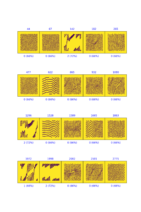
Figure 1: An application of the Carruba et al. (2021) $ANN$ model to a set of 20 images of resonant arguments of asteroids affected by the M1:2 mean-motion resonance with Mars. The number above each resonant argument is the asteroid identification, while the number at the bottom is their class, 0 for circulation, 1 for switching orbits, and 2 for librating ones), with the associated probability of the asteroid belonging to that class, as computed by the $ANN$ model.

More recently, a similar model was used by Carruba et al. (2022) to classify the orbits of asteroids affected by the ${\nu}_{6}$ secular resonance. The main difference with the Carruba et al. (2021) model was the presence of an additional class, since for ${\nu}_{6}$ asteroids libration can occur around two equilibrium points, $0^{\circ}$ (aligned libration) and $180^{\circ}$ (antialigned libration).

The main goal of this paper is to investigate how the use of more advanced model architectures can improve the classification of asteroids dynamical regimes, and how employing regularization techniques can reduce the problem of the overfitting of the training data-set. For these purposes, $CNN$s models like the VGG, Inception, and ResNet, with and without regularization techniques, will be applied to publically available resonant arguments images databases, like those for the M1:2 and ${\nu}_{6}$ resonance. Selecting the most efficient method to fit these databases, for small and large testing data-sets, will be the ultimate goal of this work.

This paper is so divided: in section (2) we revise some basic properties of $CNN$. In section  (3) we revise the architecture of some of the recently published more advanced $CNN$ models. Methods to evaluate the models’ performances will be discussed in section (4), while in section (5) we will discuss approaches to improve the models’ performances through regularization. In section (6) we will apply $CNN$ models, regularized or not, to the two asteroids’ resonant arguments images databases to select the three best performing models for each dataset. In section (7) these models will be tested with large testing sets, to ultimately select the best performing method for each set. Finally, in section (8) we will discuss our conclusions.

2 Convolutional Neural Networks, some basic concepts

Convolutional neural networks, or $CNNs$, are a type of neural network models originally designed to work with two-dimensional picture data. Their name derives from the convolutional layer, which is an important layer of the model. Convolution is a linear procedure involving the multiplication of a two-dimensional array of weights, often referred to as a filter, with an input array. This is achieved by multiplying the input and filter’s filter-sized patch element-by-element before summing the results, which produces a single value. This operation is occasionally referred to as the ”scalar product”, because it produces a single integer. Since the same filter might be multiplied by the input array several times at various points on the input, it is better to use a filter that is smaller than the input. The filter is applied sequentially from left to right and top to bottom to each overlapped piece of the input data that has the same size of the filter.

This idea of applying the same filter to an image in a systematic way is a strong concept. If a filter is designed to identify a particular type of input feature, applying the filter methodically across the entire image provides the possibility to find the feature anywhere in the data. Translation invariance, which is the name of this quality, denotes the general interest in whether a feature exists rather than its location.

The filter is multiplied once with a filter-sized piece of the input array to create a single value. When the filter is applied uniformly throughout the input array, the result is a two-dimensional array of output values that represent the input filtering. As a result, the two-dimensional output array of this procedure is referred to as a feature map. Each value in a feature map can be processed through a nonlinearity, such as a Rectified Linear Unit (ReLU), once the feature map has been built. If the input value is negative, the ReLU activation function is intended to be 0. For positive or zero values, it is intended to be the input value itself, $y=x$.

The disadvantage of convolutional layers’ feature map output is that it captures the precise location of features in the input. Even little adjustments to the position of the feature in the input image will produce a different feature map. A common solution to this issue is to utilize a pooling layer, usually added after the convolutional layer. In some models, this pattern may be repeated once or more. The pooling layer builds new pooled feature maps with the same amount of features by working separately on each feature map. In that it requires choosing a pooling procedure, pooling is comparable to applying a filter to feature maps. The pooling operation or filter, for instance, is often applied with a stride of 2 pixels and is typically smaller than the feature map.

This implies that each feature map will always be compressed by a factor of two by the pooling layer, i.e., each dimension will be halved, producing a feature map with a quarter as many pixels or values. A pooling layer applied to a 6 $\times$ 6 (36 pixels) feature map, for example, will provide a map of 3 $\times$ 3 pixels (9 pixels). Rather than being learned, the pooling operation is defined. Two common functions used for pooling operations are the average pooling, which computes the average value for each considered patch on the feature map, and the maximum pooling, where the maximum value is instead used. The result of using a pooling layer and creating downsampled or pooled feature maps is a summary of the features found in the input. Their advantage resides in the fact that even minute adjustments in the location of the feature in the input that the convolutional layer picks up will result in the feature remaining in the same location on the pooled feature map. The local translation invariance of the model is a benefit added by the pooling layer.

3 $ANN$ models

The first successful model for image classification was LeNet-5, outlined in the paper by LeCun et al. (1998). The system was created to solve a handwritten character recognition problem, and it was tested using the MNIST standard dataset, attaining a classification accuracy of about 99.2%. (or a 0.8 percent error rate). This model was subsequently characterized as the core component of a larger system known as Graph Transformer Networks.

Advancements in the field of image recognition came later on, also because of the efforts of the ImageNet project and its sponsored computer vision competition, the ImageNet Large Scale Visual Recognition Challenge (ILSVRC). The ImageNet project is a large visual database created for use in visual object recognition software research. The project has several million of images that have been hand-annotated to indicate what objects are depicted. Bounding boxes are provided for at least one million of the images. ILSVRC is an annual software contest, that has been held since 2010, where software programs compete to accurately identify and detect objects and sceneries. AlexNet refers to the model developed by Krizhevsky et al. (2012) to compete in the ILSVRC-2010 competition for the classification of objects photographs into 1000 different categories. Before the creation of AlexNet, this task was deemed to be too difficult for the then-current capacities of computer vision approaches. AlexNet success sparked a competition that inspired many more subsequent new models, several of which were applied to the same ILSVRC task of the original AlexNet problem.

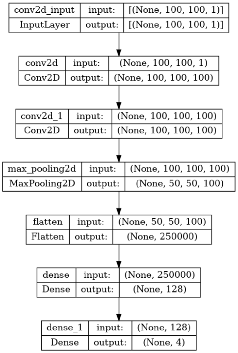
Figure 2: The architecture of the VGG model, as implemented in this work. The initial input dimension of [(None, 100, 100, 1)] refers to the dimension of the images of 100 $\times$ 100 pixels, with just one color channel (1), associated with a black and white picture. This input is fed to the first convolutional layer, that processes it and feeds its output to the next layer, until reaching the final layer with a dimension of 4, associated with the four possible classes studied in this problem, i.e., the classification of images of resonant arguments of asteroids interacting with the ${\nu}_{6}$ secular resonance.

Simonyan and Zisserman (2014) paper aimed at standardizing architecture designs for convolutional networks, while also developing better performing models. Their architecture is commonly referred to as VGG, after their lab’s name, the Visual Geometry Group at Oxford, and was developed and tested for the ILSVRC-2014 competition. Their use of several small filters has become a new standard. Most, but not all, convolutional layers are followed by max pooling layers. Another notable characteristic is the large number of filters, which rises with model depth, starting with 64 and proceeding through 128, 256, and 512 filters at the model’s feature extraction end. Among many possible architecture versions of the VGG model, two are most commonly used: the VGG-16 and VGG-19, which are named after the number of learned layers, 16 and 19, respectively. These architectures showed the best performance and depth among several VGG versions that were built and assessed. Finally, the VGG study was among the first to make model weights freely available, and this set a trend among researchers in the area of computer vision. As a result, in transfer learning, pre-trained models such as VGG are routinely employed as a starting point. The architecture of the VGG model, as defined in Brownlee (2020) and applied in this work, is shown in figure (2). Interested readers can find more details on the architecture and reasons for the choice of free parameters and number of layers of the models used in this work in Brownlee (2020).

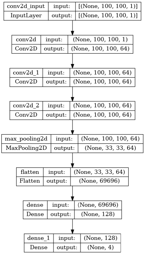
Figure 3: The architecture of the Inception model, as implemented in this work. Note the use of a stack of convolutional layers at the beginning of the architecture, typical of this model. See the text for more details on this architecture.

In their 2015 study titled Going Deeper with Convolutions, Szegedy et al. (2015) offered significant advancements in the application of convolutional layers. The authors of the paper suggested an architecture called inception and a particular network named GoogLeNet that came in first place in the ILSVRC challenge’s 2014 round. The most important innovation behind the inception models, and the main reason for their name, is the inception module. This is a stack of parallel convolutional layers with various filter sizes (such as 1 $\times$ 1, 3$\times$ 3, and 5 $\times$ 5), as well as a pooling layer with a 3 $\times$ 3 maximum, the output of which is subsequently concatenated. A problem with implementations of this model is that the filters’ number (depth or channels) starts to quickly increase in a naive implementation of the inception model, especially when inception modules are stacked. It can be computationally expensive to perform convolutions on many filters using larger filter sizes (like 3 and 5). To remedy this, 1 $\times$ 1 convolutional layers are employed before the 3 $\times$ 3 and 5 $\times$ 5 convolutional layers, as well as after the pooling layer, to reduce the number of filters in the inception model. The architecture of the Inception model, as used in this work, is shown in figure (3).

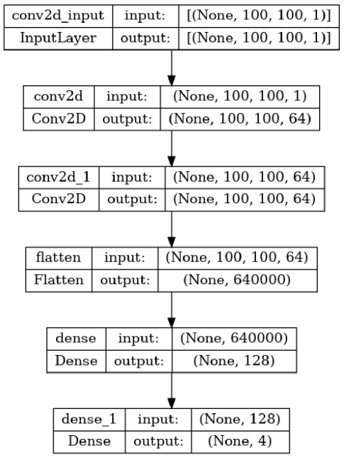
Figure 4: The architecture of the ResNet model, as implemented in this work. Note the presence of residual blocks, that are patterns comprising two convolutional layers activated by ReLU. See the text for more details on this architecture.

A Residual Network, or ResNet, was introduced by He et al. (2015) as an extremely deep model that was successful in the 2015 ILSVRC challenge. Impressively, their model has 152 layers. The concept of residual blocks that utilize shortcut connections is crucial to the architecture of the model. These are just connections where the input is transmitted to a deeper layer while remaining unchanged (i.e. skipping the following layer). A residual block is a pattern comprising two convolutional layers activated by ReLU, where the output and input of the block are combined. This is called the shortcut connection. If the input shape to the block is different from the form of the output of the block, a projected version of the input is employed. The model starts with what the authors define as a ”plain network”. Quoting Brownlee (2020), “this is a deep convolutional neural network inspired by the VGG with small filters, grouped convolutional layers that are followed by no-pooling layers, and an average pooling after the feature detector portion of the model, before an output layer with a softmax activation function”. A residual network that defines residual blocks is created by introducing shortcut connections to the plain network. The shortcut connection’s input often has the same shape as the residual block’s output. The architecture of the ResNet model is shown in figure (4).

The ResNet model was the last model revised in this work. In the next section, we are going to introduce methods to evaluate the $CNN$ models’ performance.

4 Evaluating the models’ performance

In order to evaluate the performance of deep learning models, two metrics are often used, Cross-Entropy loss (Cox, 1958) and Accuracy (Metz, 1978). Loss/cost functions are employed to optimize the model during training while working on a machine learning or deep learning problem. Almost generally, the goal is to reduce the loss function. The model performs better if the loss is lower. One of the most significant cost functions is the Cross-Entropy loss. To understand the cross entropy loss one has first to grasp the concept of the softmax activation function. The Softmax activation function is typically positioned as the deep learning model’s final layer. The activation function known as Softmax scales numbers and logits into probabilities. Softmax produces a vector (let’s say $\vec{v}$) with a probability for each potential result. For all conceivable outcomes or classes, the probabilities in vector $\vec{v}$ add up to one. The mathematical definition of Softmax is

$$S(y)_{i}=\frac{exp(y_{i})}{\sum_{j=1}^{n}exp(y_{j})},$$ (2)

where $y$ is an input vector consisting of $n$ elements for $n$ classes. Consider a CNN model that attempts to categorize a picture as either a dog, cat, horse, or cheetah (four possible results/classes). A vector of logits, L, is produced by the final (completely connected) layer of the CNN and is then sent through a Softmax layer, which converts the logits into probabilities, P. For each of the 4 classes, these probabilities represent the model predictions.

For example, let us assume that the model will classify the picture of a dog using the Softmax function with a probability 0.775 of being a dog, 0.116 for being a cat, 0.039 for being a horse, and 0.070 of being a cheetah. The goal of a deep learning model is to make the output as close as feasible to the desired result. The Cross-Entropy loss function, also called logarithmic loss, log loss or logistic loss, is defined in terms of the actual class desired output 0 or 1. A score/loss is calculated by penalizing the probability based on how different it is from the actual expected value. Because of the penalty’s logarithmic structure, significant differences close to 1 receive a large score, while minor differences close to 0 receive a small score. Mathematically, the Cross-Entropy loss function is defined as

$$L_{CE}=-\sum_{i=1}^{n}t_{i}log(p_{i}),$$ (3)

where $t_{i}$ is the truth label and $p_{i}$ is the probability for the $i-th$ class. For the case of the classification of the dog’s image, the Cross-Entropy loss function will be minimal for the case of the image being labeled as a dog, larger in the other cases, and will reach a maximum for the horse class. For the cases where we have multiple classes classification, either where the labels are integers, or one-hot-encoded, sparse categorical cross-entropy and categorical cross-entropy can be defined. Interested readers are referred to the Keras API reference (https://keras.io/api/, (Chollet and others, 2018)).

One parameter for assessing classification models is accuracy. The percentage of predictions one’s model correctly predicted is known as Accuracy. Formally, Accuracy has the following definition:

$$Accuracy=\frac{Number~{}of~{}correct~{}predictions}{Total~{}number~{}of~{}predictions}.$$ (4)

Accuracy can also be determined in terms of positives and negatives for binary classification, as seen below:

$$Accuracy=\frac{TP+TN}{TP+TN+FP+FN},$$ (5)

where $TP$ = True Positives, $TN$ = True Negatives, $FP$ = False Positives, and $FN$ = False Negatives. For the case of multiple class classification, where each class is identified by an integer label, a SparseCategoricalAccuracy can be defined. Interested readers can find more information in the Keras API reference (https://keras.io/api/, (Chollet and others, 2018)).

One of the most common limitations of deep learning models is their tendency to overfit the training data. Overfitting occurs when the neural network model learns all the minute features of the training test. While this may result in nominally excellent values of Cross-Entropy loss and Accuracy, the ability of the model to make reliable predictions on test sets different than the training one is somewhat limited. Overfitting may occur for models with a very large number of trainable parameters, or for models that trained for too long. Conversely, underfitting may occur when the train data can still be improved upon. This may occur for a variety of reasons, including inadequate model strength, excessive regularization, or insufficient training time. This indicates that the network has not picked up any useful patterns from the training data. With the latest generation of $ANN$ models, overfitting tends to be a more common occurrence than underfitting.

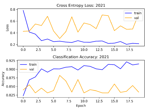
Figure 5: Cross entropy loss (top panel) and classification accuracy (bottom panel) as a function of epoch for an application of the Carruba et al. (2022) $ANN$ model. The distance between the training and validation metrics, and the fact that the accuracy for the training metric is consistently higher suggests that this model may be affected by overfitting.

A method to test for overfitting is to test the model on a validation set. A validation set is a part of the database over which the model trained on the training set can be tested. Usually, it is made of about 20% of the total database. If the model is overfitting the training set, while values of the training Cross-Entropy loss will go down and Accuracy will increase and be close to 1, the same will not be observed for these metrics applied to the validation set. Figure (5) shows a typical case where overfitting is observed. The actual performance of the model can be improved using methods such as Data Augmentation, Dropout, and Batch Normalization, which will be discussed in the next section. Generally speaking, the lower the difference between the values of Cross-Entropy loss and Accuracy of the training and validation sets, the better the actual performance of the model.

5 Improving the performance: regularization methods

There are various methods available to improve a CNN algorithm’s performance and reduce overfitting. Here we will focus on data augmentation, dropout, and batch normalization.

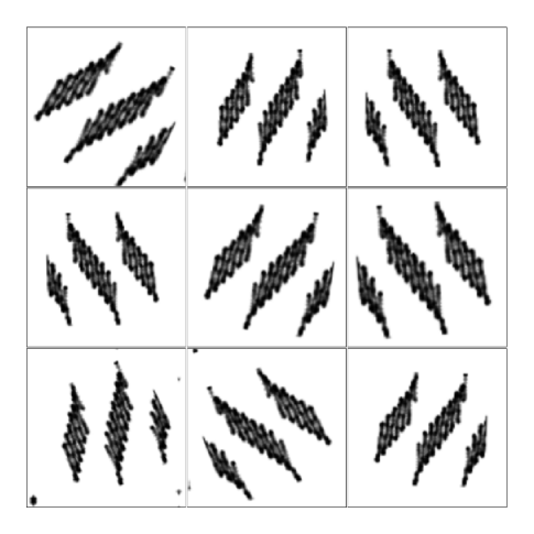
Figure 6: An example of Data Augmentation techniques applied to an image in the ${\nu}_{6}$ database. We applied three instances each of a random flip, random rotation and random zoom.

Data augmentation entails creating duplicates of the training dataset’s samples with minor random changes. This has a regularizing effect by allowing the model to learn the same broad features but in a more generic way while also expanding the training dataset. A variety of data augmentation techniques could be used. Given that the datasets that we are going to investigate consist of tiny images of resonant arguments, we will not use augmentation that severely distorts the images in order to preserve and utilize relevant information. The kinds of random augmentations that might be helpful include flipping an image horizontally, making modest image shifts, and possibly making minor zooming or cropping adjustments. Figure (6) displays an example of data augmentation obtained with the ImageDataGenerator class in Keras for an image from the ${\nu}_{6}$ database (see section (6) for more details on the use and applications of this dataset). Our example includes basic augmentations, such as flipping the image horizontally and shifting its height and breadth by 10%.

Dropout is a straightforward method that will erratically remove nodes from the network. As the remaining nodes must adjust to fill in the gaps left by the eliminated nodes, it has a regularizing effect. By including new dropout layers to the model, where the number of nodes deleted is controlled by a parameter, dropout can be added. In terms of where to add the layers and how much dropout to utilize, there are numerous patterns for adding dropouts to a model. In our case, we will use a fixed dropout rate of 20%, and add dropout layers after each max pooling layer and after the fully connected layer.

Finally, another method to reduce overfitting is batch normalization. Brownlee (2020) defines this method as “a technique for training very deep neural networks that standardizes the inputs to a layer for each mini-batch. This has the effect of stabilizing the learning process and dramatically reducing the number of training epochs required to train deep networks.”

Batch normalization employs a transformation that keeps the output mean and standard deviation close to 0 and to 1, respectively. Interested readers can find more information on the method in Brownlee (2020), here we will use batch normalization as implemented in Keras (https://keras.io/api/,
Chollet and others (2018)).

6 Applications to images databases

The use of $ANN$ for the purpose of classification of images of asteroid resonant arguments started in 2021 with the work of Carruba et al. (2021), where images of the resonant arguments of 6440 asteroids affected by the M1:2 exterior mean-motion resonance with Mars were classified, and the dynamical regimes identified within three categories (libration, circulation, and orbits switching from one mode to the other). Figure (7) displays the architecture of the 2021 $ANN$ model.

More recently, the same model was used by Carruba et al. (2022) to classify the orbits of more than 10000 asteroids affected by the ${\nu}_{6}$ secular resonance into four classes, circulation, aligned libration, where the resonant argument oscillates around $0^{\circ}$, antialigned libration, with oscillations around $180^{\circ}$, and switching behavior. Both databases of asteroids’ resonant arguments are publically available on the authors’ research group server.

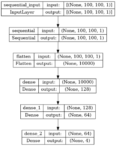
Figure 7: The architecture of the Carruba et al. (2022) $ANN$ model.

The model proposed in 2021 allowed to speed up the classification of asteroidal images, but it has some limitations. Considering the ${\nu}_{6}$ database, if we set aside a sample of 4875 asteroids images of numbered asteroids as a training set, and a sample of 1350 numbered asteroids with identifications between 523584 and 607011, we obtained Cross entropy loss and classification accuracy as a function of the epoch, for 20 epochs. Figure (5) shows our results, that are clearly affected by overfitting.

In this work, we will explore how the use of three more advanced models, the VGG, Inception, and ResNet architecture (see figures (2, 3, 4) for a summary of their architectures, as used in this work), improved by the regularization techniques seen in section (5), can boost the performance of image recognition for these kinds of problems.

To quantitatively compare the outcome of the different models tested in this work, we also computed the elapsed time needed to fit all models over 20 epochs, and the mean and maximum memory allocation during this process. All simulations ran alone on a Xubuntu workstation with an Intel I9-10900 processor with a DDR4 16GB 3200Mhz net core memory. We will start our analysis by studying the ${\nu}_{6}$ database.

6.1 Asteroids affected by the ${\nu}_{6}$ resonance

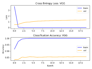
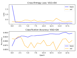
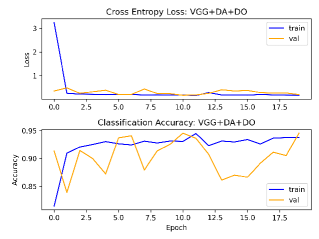
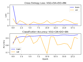
Figure 8: Cross entropy loss and classification accuracy as a function of epoch for the VGG model (top left panel), the VGG model plus data Augmentation (DA, top right panel), the VGG model plus DA and Dropout (DA+DO, bottom left panel), and also including Batch Normalization (DA+DO+BN, bottom right panel). Results obtained for the ${\nu}_{6}$ database.

As the first step in our analysis, we will use the ${\nu}_{6}$ asteroid database with the training, test, and validation structure described at the end of section (6). The first model applied to this dataset was the VGG, and was implemented alone and i) with data augmentation (DA), ii) data augmentation and dropout (DA+DO), and, finally, iii) also including batch normalization (DA+DO+BN). Our results are shown in figure (8), in the Appendix.

The results of the VGG model alone are clearly affected by overfitting. DA improves the outcome of the Cross entropy loss function, but accuracy is still not optimal. Better results are obtained when both DA and DO are applied, and they are not much improved if we also use BN.

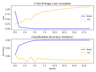
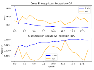
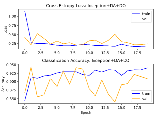
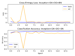
Figure 9: The same as in figure (8), but for the outcome of the Inception models.

For the case of the Inception model (see figure (9), in the appendix), again, we observe overfitting for the model alone without regularizations. The situation improves significantly for models with DA and DO, and there is almost no overfitting if we also consider BN. However, in this case, values of Accuracy are significantly lower than for what was observed for the DA+DO case.

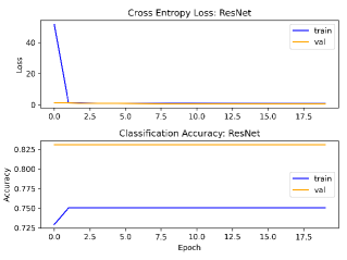
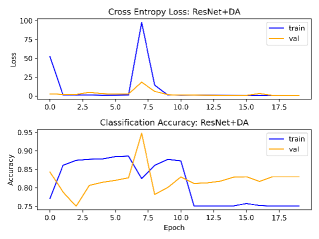
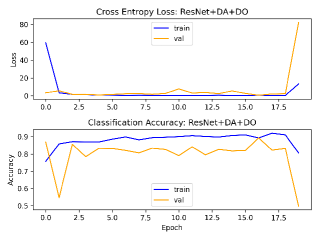
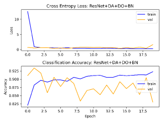
Figure 10: The same as in figure (8), but for the outcome of the ResNet models.

Finally, for the ResNet model (see figure (10), in the appendix) we actually observe underfitting for the model alone. The best results are again obtained for the model with DA+DO.

Table 1: Execution time, memory and maximum memory allocation for the models tested in this work for the ${\nu}_{6}$ database.

Model	Time	Memory	Max. Memory
	[h:m:s]	alloc. [Bytes]	alloc. [Bytes]
VGG	0:25:52.6	3633632	194524205
VGG+DA	0:25:14.1	4951169	194528646
VGG+DA+DO	0:11:41.7	5157584	194526710
VGG+DA+DO+BN	0:13:02.8	5185155	194527529
Inception	0:26:27.0	5746597	194896854
Inception+DA	0:27:47.7	5883557	194924103
Inception+DA+DO	0:28:27.4	5863357	194940207
Inception+DA+DO+BN	0:29:29.2	6388938	195023989
ResNet	0:17:13.1	4142248	331982732
ResNet+DA	0:16:50.2	5735049	333427831
ResNet+DA+DO	0:19:43.4	5655480	333496679
ResNet+DA+DO+BN	0:21:30.1	5824092	333666545

Our results in terms of execution time and memory allocation are reported in the table (1). The three best performing models in terms of avoidance of overfitting, execution time, and memory allocation were the VGG, ResNet, and Inception regularized with Data Augmentation and Dropout. For the case of the Inception model, better results in terms of overfitting were obtained for the case that also includes Batch Normalization, but values of accuracy were better for the model with just DA and DO.

In the next subsection, we will analyze the case of the M1:2 resonance database.

6.2 Asteroids affected by the M1:2 resonance

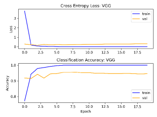
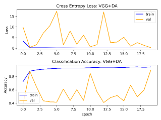
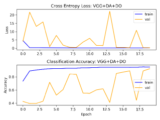
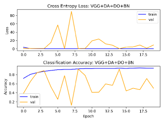
Figure 11: Cross entropy loss and classification accuracy as a function of epoch for the VGG model (top left panel), the VGG model plus data Augmentation (DA, top right panel), the VGG model plus DA and Dropout (DA+DO, bottom left panel), and also including Batch Normalization (DA+DO+BN, bottom right panel). Results obtained for the M1:2 database.

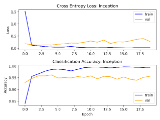
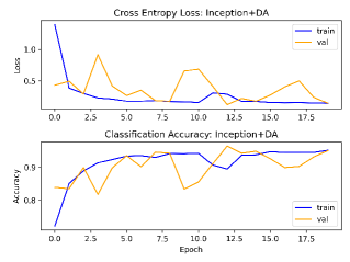
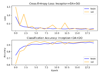
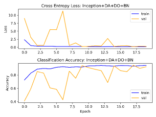
Figure 12: The same as in figure (11), but for the outcome of the Inception models.

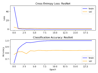
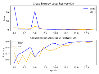
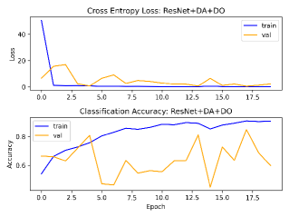
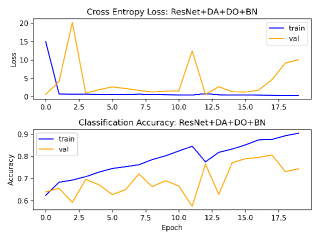
Figure 13: The same as in figure (11), but for the outcome of the ResNet models.

The Carruba et al. (2021) database contains images of 5700 asteroids’ resonant arguments. This dataset was divided into 4560 images for training (80% of the total) and 1140 images for validation (20% of the total), with 100 images used for the test set. The same models discussed in section (6.1) were applied to this database, with the only difference that the last Dense layer had 3 nodes instead of 4, since there are only three possible classes for this set. Our results for the VGG, Inception, and ResNet models, without and with the three regularizations (DA, DO, BN) are shown in the appendix, in figures (11, 12, 13). Table (2) displays our results in terms of execution time and memory allocation.

The best performing model in terms of overfitting avoidance was the Inception, regularized with Data Augmentation and Dropout. Surprisingly, the second-best performance was obtained by the VGG model with no regularization. Finally, the third best model was ResNet, regularized with DA, DO, and BN. In the next section, we will review how these models perform for larger test databases.

Table 2: Execution time, memory and maximum memory allocation for the models tested in this work for the M1:2 database.

Model	Time	Memory	Max. Memory
	[h:m:s]	alloc. [Bytes]	alloc. [Bytes]
VGG	0:24:32.0	4744976	183469190
VGG+DA	0:24:16.0	5186968	196222507
VGG+DA+DO	0:25:22.7	5947897	194526710
VGG+DA+DO+BN	0:28:37.3	5368555	183121859
Inception	0:24:55.8	4725164	183486485
Inception+DA	0:25:18.7	6094216	183512476
Inception+DA+DO	0:25:25.3	6311918	183519955
Inception+DA+DO+BN	0:27:18.3	6467734	183605621
ResNet	0:15:53.6	4653649	332345991
ResNet+DA	0:16:19.3	5153001	379370007
ResNet+DA+DO	0:18:40.8	6006420	333848121
ResNet+DA+DO+BN	0:19:35.9	6178250	334018955

7 Applications to larger test datasets

In the previous section, we trained our models with large testing and validation sets, but with small testing ones. Here, the three best-performing models selected in the previous section are tested on larger databases for both the ${\nu}_{6}$ and M1:2 resonances. For the case of the ${\nu}_{6}$ secular resonance, we consider a set of 3000 asteroid resonant arguments’ images obtained by Carruba et al. (2022) for multi-opposition asteroids affected by this resonance. For the M1:2 resonance, we selected 650 numbered objects with identifications larger than 523584 and lower than 606158 that were not previously considered by Carruba et al. (2021).

To assess the performance of the models, we used the accuracy, as defined in equations (4) and (5), and the F-beta score. The F-beta score is a metric, commonly used for binary classification problems, which is based on precision and recall. The percentage of accurate predictions for the positive class is calculated using the precision metric, which is given by:

$$precision=\frac{TP}{TP+FP}.$$ (6)

Recall, defined as:

$$recall=\frac{TP}{TP+FN},$$ (7)

determines the proportion of accurate positive predictions for the positive class out of all possible positive predictions. While maximizing recall will reduce false-negative errors, maximizing precision will reduce false-positive mistakes.

The harmonic mean of precision and recall is used to calculate the F-measure, giving each the same weight. This makes it possible to compare models and describe a model’s performance while also accounting for both precision and recall in a single score. A generalization of the F-measure, called the F-beta-measure includes a beta configuration parameter. For the F-measure this is equal to 1.0, which serves as the default beta value. In the calculation of the score, a smaller beta value, such as 0.5, gives more weight to recall and less to precision, whereas a greater beta value, such as 2.0, gives less weight to recall and more weight to precision. Following Brownlee (2020), we can define F-beta as:

$${F-beta}=(1+beta^{2})\times\frac{precision\times recall}{beta^{2}\times precision+recall}$$ (8)

Interested readers can find more information on the F-beta score in Brownlee (2020), chapter 22. Here, we are using the F-beta score as introduced by Pedregosa et al. (2011), and as implemented in the scikit-learn API Buitinck et al. (2013), with a beta value of 0.5, to give more weight to recall. Also, since we are dealing with a multi-class imbalanced problem, we used the ’weighted’ option of the average parameter, which will calculate metrics for each label and find their average weighted by their support, i.e., the number of true instances for each label. For more details on this last procedure please see Pedregosa et al. (2011).

Our results for the two datasets are shown in table (3). We included in our runs two versions of the VGG model, with and without regularizations, since the unregularized VGG model was one of the best performing for the M1:2 database, and we wanted to check its behavior for both cases. The best performing models for the ${\nu}_{6}$ and M1:2 resonances were the VGG, with and without regularization, with the Inception models performing slightly worse, followed by the ResNet models as a distant third.

Table 3: Values of accuracy and F-beta for the best performing models selected in section (6.1) and (6.2).

Database	Model	Accuracy	F-beta
${\nu}_{6}$	VGG	0.842	0.818
${\nu}_{6}$	VGG+DA+DO	0.884	0.872
${\nu}_{6}$	Inception+DA+DO	0.814	0.878
${\nu}_{6}$	ResNet+DA+DO	0.760	0.659
M1:2	VGG	0.935	0.937
M1:2	VGG+DA+DO	0 849	0.850
M1:2	Inception+DA+DO	0.882	0.890
M1:2	Resnet+DA+DO+BN	0.562	0.587

8 Conclusions

The main objective of this paper was to identify which approach, among modern available $CNN$ models, was i) less prone to overfitting, and ii) more efficient in predicting the labels of large datasets of asteroids’ resonant images. Using two publically available datasets of images of asteroids resonant arguments for objects interacting with the ${\nu}_{6}$ and M1:2 resonances, and setting aside a validation set for both databases, we identified three best performing models for each dataset, corrected (or not) for overfitting using standard regularization methods such as Data Augmentation, Dropout, and Batch Normalization, or combinations of such methods.

These best-performing methods were then tested on larger testing datasets, containing up to 3000 images of asteroidal resonant arguments. Their performance was measured using the standard accuracy metric, and the weighted F-beta score, a metric apt to measure the model efficiency for multi-class imbalanced problems, like the ones studied in this work. Surprisingly, the simplest method, the VGG, with or without regularization, performed best for both cases. Such models, which run in seconds on our machine, can now be used to classify thousands of asteroidal images of resonant arguments with accuracies and F-beta scores of up to 93.5%, and they will prove themselves quite valuable when the Vera C. Rubin surveys will start to discover millions of new asteroids after the beginning of operations (Jones et al., 2015).

Obtaining databases for other resonances interacting with asteroidal populations and performing an optimization study like the one carried out in this work remain challenges for future research.

9 Appendix: $CNN$ model performances results

In this appendix, we report plots of cross entropy loss and classification accuracy for the models tested on the ${\nu}_{6}$ and M1:2 images databases. See the discussion in sections (6.1) and (6.2) for more information on how to interpret these figures.

Conflict of interest

The authors declare that they have no conflict of interest.

10 Author contributions

All authors contributed to the study conception and design. Material preparation, and data collection were performed by Valerio Carruba, and Safwan Aljbaae. The first draft of the manuscript was written by Valerio Carruba and all authors commented on previous versions of the manuscript. All authors read and approved the final manuscript.

11 Data availability

The images database for the ${\nu}_{6}$ resonance was published in Carruba et al. (2022) and is available at this link:

https://drive.google.com/drive/folders/
1oxdXquibdYYP965AgzoMjFop-ZZXcHni

With the exception of the images used for the testing set in section  (7), the database for the M1:2 resonance was published in Carruba et al. (2021) and is available at:

https://drive.google.com/file/d/
1RsDoMh8iMwZhD-fnkYSs9hiWmg96SZf0/
view?usp=sharing

The testing set of images for M1:2 resonance used in section (7) can be obtained from the first author upon reasonable request.

12 Code availability

The codes developed for this work are publically available at this GitHub repository:

https://github.com/valeriocarruba/CNN-Optimization

References

- Brownlee (2020) Brownlee J (2020) Deep Learning for Computer Vision: Image Classification, Object Detection, and Face Recognition in Python. Ed. Machine Learning Mastery, San Juan, PR, USA
- Buitinck et al. (2013) Buitinck L, Louppe G, Blondel M, Pedregosa F, Mueller A, Grisel O, Niculae V, Prettenhofer P, Gramfort A, Grobler J, Layton R, VanderPlas J, Joly A, Holt B, Varoquaux G (2013) API design for machine learning software: experiences from the scikit-learn project. In: ECML PKDD Workshop: Languages for Data Mining and Machine Learning, pp 108–122
- Carruba et al. (2021) Carruba V, Aljbaae S, Domingos RC, Barletta W (2021) Artificial neural network classification of asteroids in the M1:2 mean-motion resonance with Mars. MNRAS504(1):692–700, DOI 10.1093/mnras/stab914, 2103.15586
- Carruba et al. (2022) Carruba V, Aljbaae S, Domingos RC, Huaman M, Martins B (2022) Identifying the population of stable 6 resonant asteroids using large data bases. MNRAS514(4):4803–4815, DOI 10.1093/mnras/stac1699, 2203.15763