The two-photon decay of X(6900) from light-by-light scattering at the LHC

Abstract

The LHCb Collaboration has recently discovered a structure around 6.9 GeV in the double-$J/\psi$ mass distribution, possibly a first fully-charmed tetraquark state $X(6900)$. Based on vector-meson dominance (VMD) such a state should have a significant branching ratio for decaying into two photons. We show that the recorded LHC data for the light-by-light scattering may indeed accommodate for such a state, with a $\gamma\gamma$ branching ratio of order of $10^{-4}$, which is larger even than the value inferred by the VMD. The spin-parity assignment $0^{-+}$ is in better agreement with the VMD prediction than $0^{++}$, albeit not significantly at the current precision. Further light-by-light scattering data in this region, clarifying the nature of this state, should be obtained in the Run 3 and probably in the high-luminosity phase of the LHC (Run 4 etc.).

I Introduction

The ATLAS and CMS Collaborations have recently made first experimental observations of light-by-light (LbL) scattering in the ultra-peripheral Pb-Pb collisions at the LHC Aaboud et al. (2017); Sirunyan et al. (2019). The ATLAS Collaboration has subsequently provided the most comprehensive dataset from the LHC Run-2 Aad et al. (2021), which shows a mild excess over the Standard Model prediction centered on the diphoton invariant mass region of 5 to 10 GeV (cf. Fig. 2 below). A similar excess between 5-7 GeV of the diphoton invariant mass was seen by CMS Collaboration Sirunyan et al. (2019) as well.

More recently, the LHCb Collaboration has observed a structure in the di-$J/\psi$ mass distribution LHCb collaboration (2020) and interpreted it as a new state, $X(6900)$, with mass and di-$J/\psi$ width quoted in Table 1. This state is possibly the lightest fully-charmed tetraquark state Richard (2020); Sonnenschein and Weissman (2021); Faustov et al. (2021); Deng et al. (2021); Guo and Oller (2021) (see also Chen et al. (2022) for review), and according to Refs. Karliner and Rosner (2020); Debastiani and Navarra (2019); Liu et al. (2020); Lü et al. (2020); Wu et al. (2018); Bedolla et al. (2020); Wang et al. (2019); Wan and Qiao (2021); Liang et al. (2021); Li et al. (2021); Ke et al. (2021) can be a pseudoscalar $P$-wave state ($J^{PC}=0^{-+}$), or a scalar $S$-wave state ($J^{PC}=0^{++}$). A possibility for it to be a tensor meson ($J^{PC}=2^{++}$) is discussed in Chen et al. (2022); Faustov et al. (2021); Deng et al. (2021); Karliner and Rosner (2020); Lü et al. (2020); Bedolla et al. (2020); Liang et al. (2021); Li et al. (2021); Ke et al. (2021); Weng et al. (2021); Zhu (2021). In any of these cases, this state would likely couple to two photons and hence contribute to the LbL scattering. In fact, the vector-meson dominance (VMD) hypothesis provides a rather accurate prediction for the two-photon decay width ($X\to\gamma\gamma$) in terms of the di-$J/\psi$ width (cf. Appendix).

Parameter	Interference	No-interference
$m_{X}$ [MeV]	$6886\pm 11\pm 11$	$6905\pm 11\pm 7$
$\Gamma_{X\rightarrow J/\psi J/\psi}$ [MeV]	$168\pm 33\pm 69$	$80\pm 19\pm 33$
$\Gamma_{X\rightarrow\gamma\gamma}$ [keV]	$67^{+15}_{-19}$	$45^{+11}_{-14}$

Table 1: The mass and di-$J/\psi$ width of $X(6900)$ in the two scenarios of Ref. LHCb collaboration (2020), and the corresponding two-photon widths obtained here by fitting the light-by-light scattering data of Ref. Aad et al. (2021).

In this work we explore the possibility of the excess seen in ATLAS experiment is due to the $X(6900)$ meson. The two-photon decay width of this state can then be determined from a fit to the data, with the resulting values shown in the last row of Table 1. In what follows we describe our formalism for the inclusion of mesons in LbL scattering (Sec. II), the details and results of the fit to ATLAS data (Sec. III), comparison with VMD estimates (Sec. IV), and conclusions (Sec. V).

II Meson exchange in light-by-light scattering

We start with outlining the formalism for the inclusion of meson states into the LbL process. These states ought to be added at the amplitude level. It is conventional to work with helicity amplitudes $M_{\lambda_{1}\lambda_{2}\lambda_{3}\lambda_{4}}(s,t,u)$, where $\lambda_{i}=\pm 1$ is the helicity of each of the four photons and the Mandelstam variables of the LbL scattering satisfy the kinematic constraint: $s+t+u=0$. Thanks to the discrete ($P$, $T$, $C$) symmetries only 5 of the 16 amplitudes are independent, e.g.: $M_{++++}$, $M_{+--+}$, $M_{+-+-}$, $M_{+++-}$ and $M_{++--}$. Furthermore, the crossing symmetry infers the following relation:

$$M_{++++}(s,t,u)=M_{+--+}(t,s,u)=M_{+-+-}(u,t,s).$$ (1)

The remaining two amplitudes are fully crossing invariant.

In what follows we consider spin-0 mesons, with parity $P=+$ (scalars) or $P=-$ (pseudoscalars). Their tree-level contributions to the LbL amplitudes follow from a simple effective Lagrangian (cf. Appendix), yielding the following expressions:

$$M^{P}_{++++}(s,t,u)=-\frac{16\pi s^{2}\Gamma_{\gamma\gamma}}{m^{3}\,(s-m^{2})},$$ (2a)

$$M^{P}_{+++-}(s,t,u)=0,$$ (2b)

$$M^{P}_{++--}(s,t,u)$$

$$\quad=-P\frac{16\pi\Gamma_{\gamma\gamma}}{m}\left(\frac{s}{s-m^{2}}+\frac{t}{t-m^{2}}+\frac{u}{u-m^{2}}\right),$$ (2c)

where $P=\pm 1$ stands for the parity of the state, $m$ for the mass, and $\Gamma_{\gamma\gamma}$ for the two-photon width.

The nonvanishing amplitudes are precisely the ones entering the forward LbL scattering sum rules Pascalutsa and Vanderhaeghen (2010), and it is useful to check the consistency of the above expressions with the sum rules. We recall that the helicity amplitudes of the forward ($t=0$) [or, equally, the backward ($u=0$), scattering of real photons satisfy exact sum rules Pascalutsa and Vanderhaeghen (2010); Pascalutsa (2018):

$$M_{++++}(s)+M_{+-+-}(s) =\frac{2s^{2}}{\pi}\int\limits_{0}^{\infty}ds^{\prime}\frac{\sigma_{0}(s^{\prime})+\sigma_{2}(s^{\prime})}{s^{{}^{\prime}2}-s^{2}-i0^{+}},$$ (3a)

$$M_{++++}(s)-M_{+-+-}(s) =\frac{2s}{\pi}\int\limits_{0}^{\infty}ds^{\prime}\,\frac{s^{\prime}\left[\sigma_{0}(s^{\prime})-\sigma_{2}(s^{\prime})\right]}{s^{{}^{\prime}2}-s^{2}-i0^{+}},$$ (3b)

$$M_{++--}(s) =\frac{2s^{2}}{\pi}\int\limits_{0}^{\infty}ds^{\prime}\frac{\sigma_{\parallel}(s^{\prime})-\sigma_{\perp}(s^{\prime})}{s^{{}^{\prime}2}-s^{2}-i0^{+}}.$$ (3c)

where the right-hand side involves integrals of total $\gamma\gamma$-fusion cross sections for various photon polarizations. For the case of $\gamma\gamma$-fusion into a scalar or a pseudoscalar meson these cross sections take the following simple form (see, e.g., Budnev et al. (1975); Pascalutsa et al. (2012)):

$$\sigma_{0}(s)=16\pi^{2}\frac{\Gamma_{\gamma\gamma}}{m}\,\delta(s-m^{2}),\quad\sigma_{2}(s)=0,$$ (4a)

$$\begin{cases}\sigma_{\parallel}(s)=\sigma_{0}(s),\quad\sigma_{\perp}(s)=0,\quad\text{for scalar},\\ \sigma_{\perp}(s)=\sigma_{0}(s),\quad\sigma_{\parallel}(s)=0,\quad\text{for pseudoscalar}.\end{cases}$$ (4b)

Substituting these cross sections into the sum rules we find that the contribution to $M_{++++}$ found in Eq. (2a) is reproduced by the first sum rule, but not the second one. This inconsistency can be fixed by reducing the one power of $s$ in the expression (2a), thus resulting in:

$$M^{P}_{++++}(s,t,u)=-\frac{16\pi s\,\Gamma_{\gamma\gamma}}{m\,(s-m^{2})}.$$ (5)

This contribution is consistent with both sum rules and has a better energy behavior. We shall use it in place of Eq. (2a).

The contribution to $M_{++--}$ in Eq. (2c) is consistent with the sum rule (3c). As a side remark we note that it satisfies a more general off-forward sum rule:

$$M_{++--}(s,t,u) = \frac{1}{\pi}\int\limits_{0}^{\infty}ds^{\prime}\big{[}\sigma_{\parallel}(s^{\prime})-\sigma_{\perp}(s^{\prime})\big{]}$$ (6)

$$\times \Big{(}\frac{s}{s^{\prime}-s}+\frac{t}{s^{\prime}-t}+\frac{u}{s^{\prime}-u}\Big{)}.$$

Any single-meson-exchange contribution to this LbL scattering should satisfy this sum rule. However it does not hold in a more general case — a subtraction function must be added. A similar off-forward sum rule holds for the crossing-invariant combination $M_{++++}+M_{+--+}+M_{+-+-}$ and the unpolarized cross section of $\gamma\gamma$ fusion. It also holds without subtraction for the single-meson-exchange contributions.

Next step is the inclusion of the decay width. It can be done by resumming the meson self-energy, $\Pi(s)$, in $s$-channel exchange contribution, such that the factors $1/(s-m^{2})$ in the above expressions are replaced with $1/\big{(}s-m^{2}-\Pi(s)\big{)}$. The decay width then comes from the imaginary part of the self-energy, i.e., $\mathop{\mathrm{Im}}\,\Pi(s)=-\sqrt{s}\,\Gamma(s)$. The real part of the self-energy contributes to the mass and field renormalization; any further effects of the real part are neglected here. For the total decay width of $X(6900)$-meson we use below the energy-dependent di-$J/\psi$ width, as calculated in the Appendix.

III Fitting $X(6900)$ into the light-by-light data

We have extended the Monte-Carlo code SuperChic v3.05 Harland-Lang et al. (2019, 2016) used in the original interpretation of the ATLAS data Aad et al. (2021), by including the $X(6900)$ along with the well-known bottomonium states Wang et al. (2018) pertinent to this energy region, see Table 2. Note that SuperChic v3.05 includes otherwise only the simplest perturbative-QCD (pQCD) contributions to LbL scattering, i.e., the quark-loop contribution. The next-to-leading order pQCD corrections were shown to contribute at the order of few percent Bern et al. (2001); Kłusek-Gawenda et al. (2016); Krintiras et al. (2022), which is negligible at the current level of experimental precision.

Meson	$J^{PC}$	$M$, [MeV]	$\Gamma_{\mathrm{tot}}$, [MeV]	$\Gamma_{\gamma\gamma}/\Gamma_{\mathrm{tot}}$ [%]
$\eta_{b}$(1S)	$0^{-+}$	$9399.0$	$17.9$	$5.87\times 10^{-3}$
$\eta_{b}$(2S)	$0^{-+}$	$9999.0$	$8.34$	$5.86\times 10^{-3}$
$\chi_{b0}$(1P)	$0^{++}$	$9859.44$	$3.39$	$5.87\times 10^{-3}$
$\chi_{b0}$(2P)	$0^{++}$	$10232.5$	$3.54$	$5.41\times 10^{-3}$

Table 2: Bottomonium resonances included in this work.

Given the mass and width of $X(6900)$ from the LHCb determination, the two-photon-decay width can be determined from the ATLAS data on LbL scattering. In the narrow resonance approximation, the LbL cross section depends only on the ratio $\Gamma_{X\to\gamma\gamma}/\sqrt{\Gamma_{\mathrm{tot}}}$, and hence we take it as a fitting parameter. The total width is assumed to be dominated by the di-$J/\psi$ decay (i.e., $\Gamma_{\mathrm{tot}}\simeq\Gamma_{X\to J/\psi\,J/\psi}$).

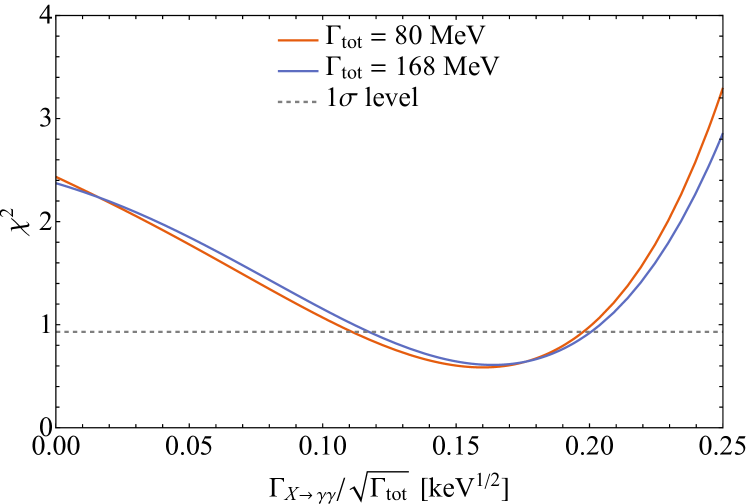
Figure 1: The profile of $\chi^{2}$ (divided by #d.o.f. = 3) for the values of $\Gamma_{\mathrm{tot}}$ used in the two LHCb scenarios. The gray dashed line cuts out the $1\sigma$ interval.

The fit has been performed to the unfolded diphoton invariant mass spectrum of the ATLAS data. The CMS data is not used in the present analysis since the corresponding spectrum is not unfolded. We have explored both the scalar and pseudoscalar nature of $X(6900)$, but the corresponding results of the fit turn out to be indistinguishable at the current level of statistical accuracy. We therefore show only the results for the scalar $X(6900)$. Since the main uncertainties in ATLAS data has a statistical origin, then for reasons of simplicity we take the total experimental uncertainties as the uncertainties for $\chi^{2}$ function. The resulting $\chi^{2}$ is shown in Fig. 1, for the two scenarios provided by the LHCb experiment. The best fit yields the following branching ratio ($\Gamma_{X\to\gamma\gamma}/\Gamma_{\mathrm{tot}}$):

$$B(X\to\gamma\gamma)=\begin{cases}5.6^{+1.3}_{-1.6}\times 10^{-4},&\text{No-int. sc},\\ 4.0^{+0.9}_{-1.1}\times 10^{-4},&\text{Int. sc.}.\end{cases}$$ (7)

The corresponding values for the $\gamma\gamma$ decay width are given in the last row of Table 1.

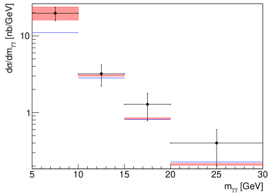
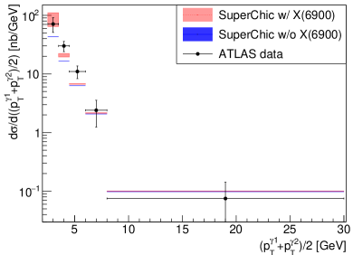
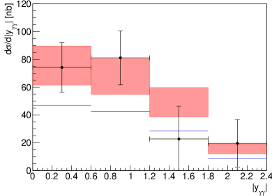
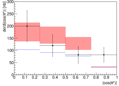
Figure 2: Differential fiducial cross sections of $\gamma\gamma\rightarrow\gamma\gamma$ production in Pb$+$Pb collisions at a centre-of-mass energy of $\sqrt{s_{NN}}=5.02$ TeV with integrated luminositiy 2.2 nb^-1 for four observables (from left to right and top to bottom): diphoton invariant mass $m_{\gamma\gamma}$, diphoton absolute rapidity $|y_{\gamma\gamma}|$, average photon transverse momentum $(p_{T}^{\gamma_{1}}+p_{T}^{\gamma_{2}})/2$ and diphoton $|cos(\theta^{\ast})|\equiv|\tanh(\Delta y_{\gamma_{1},\gamma_{2}}/2)|$. The red band represents an uncertainty ($1\sigma$ range) of the fit with $X(6900)$. The blue band contains only the statistical uncertainty of the SuperChic simulation without $X$-resonance.

Figure 2 shows the exclusive differential cross sections with and without the inclusion of $X(6900)$, versus the the ATLAS data Aad et al. (2021). The statistical uncertainties of the SuperChic results were highly reduced by simulating a large enough number of events ($10^{4}$), thus they were neglected in analysis and are not visible on the plots of Fig. 2. The fit yields the integrated fiducial cross section of $\sigma^{X}_{\mathrm{fid}}=121\pm 20$ nb. It can be compared with the reference SuperChic value without $X$-resonance, $\sigma^{0}_{\mathrm{fid}}=76$ nb and with the experimental value, $\sigma^{\mathrm{exp.}}_{\mathrm{fid}}=120\pm 17\mathrm{(stat.)}\pm 13\mathrm{(syst.)}\pm 4\mathrm{(lumi.)}$ nb, reported by ATLAS Aad et al. (2021). The description of ATLAS data with $X(6900)$ is better than without it by about $2.3\sigma$.

IV Vector-meson-dominance estimate

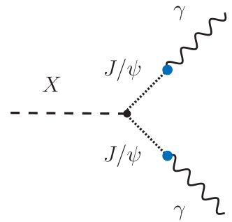
Figure 3: The $X(6900)\to\gamma\gamma$ decay via the VMD mechanism.

The ratio $\Gamma_{X\to\gamma\gamma}/\Gamma_{X\to J/\psi J/\psi}$ can be estimated via the VMD mechanism shown in Fig. 3. As the result, we obtain the following estimate for branching ratios in the scalar and pseudoscalar case, respectively (cf. Appendix for details):

$$B^{\mathrm{S}}_{\mathrm{VMD}}(X\to\gamma\gamma)=(2.8\pm 0.4)\times 10^{-6},$$ (8a)

$$B^{\mathrm{PS}}_{\mathrm{VMD}}(X\to\gamma\gamma)=(6.4\pm 0.8)\times 10^{-6}.$$ (8b)

As one can see, the central values of this estimate is about two orders of magnitude smaller than we obtained from the fit, Eq. (7); although, given the large uncertainties, the difference is fairly insignificant.

Certainly, further measurements of both the di-$J/\psi$ and $\gamma\gamma$ channels are desirable to pin down this possible inconsistency with the VMD expectations. It could perhaps be explained by other exotic resonances in the diphoton mass region from 5 to 10 GeV, which contribute to the observed excess on the $\gamma\gamma$ channel. The broad $X(6900)$ structure has already been proposed to be associated with more than one tetraquark states Barnea et al. (2006); Berezhnoy et al. (2012); Karliner et al. (2017); Wang (2017); Liu et al. (2019); Weng et al. (2021); Lundhammar and Ohlsson (2020); a second resonance could be located at around $7.2$ GeV, see e.g., LHCb collaboration (2020); Sonnenschein and Weissman (2021); Wan and Qiao (2021); Zhu (2021); Liang et al. (2021).

V Conclusion and Outlook

We have shown that the new tetraquark state $X(6900)$, observed by LHCb Collaboartion in the di-$J/\psi$ channel, could, in principle, account for the excess in the light-by-light scattering seen in the ATLAS and CMS data, The inclusion of $X(6900)$ improves the Standard Model prediction in the corresponding diphoton mass region of LbL cross sections. The $X\to\gamma\gamma$ branching ratio has been fitted to the ATLAS data. The result seen in Eq. (7), however, exceeds the VMD expectations, albeit statistically the discrepancy is not severe. Further measurements of the LbL scattering in the 5 to 10 GeV diphoton-mass range are very desirable to improve the precision.

Going to lower diphoton masses and increasing the statistics of the $\gamma\gamma\rightarrow\gamma\gamma$ events in future runs of the LHC will crucially improve the precision of the fit and hence further constrain the properties of the $X(6900)$. Moreover, the prospective double-differential (or even triple-differential) measurements of a pair (or triplet) of the observables depicted in Fig. 2, which show complementary sensitivity to $X$-state, may provide an additional improvement. Furthermore, since the Landau-Yang theorem forbids the exchange of the spin-1 $X$-resonance, the analysis of real $\gamma\gamma\rightarrow\gamma\gamma$ scattering ought to reduce the amount of possible quantum numbers of $X(6900)$, which are considered in several analyses (see, e.g. Liu et al. (2019, 2020)). Future measurements at LHCb that will allow the partial-wave analysis, could also narrow down the set of possible quantum number configurations.

Appendix A Branching ratio estimate using VMD

We estimate the two-photon decay width of $X(6900)$ by exploiting the vector meson dominance (VMD) hypothesis as shown in Fig. 3. The VMD implies that the photon $\lvert\gamma\rangle$ couples via a vector-meson state $\lvert V\rangle$ as follows Barger and Phillips (1975); Redlich et al. (2000):

$$\lvert\gamma\rangle\to\frac{e}{M_{V}}f_{V}\lvert V\rangle,$$ (A.1)

where $e$ is the electron charge, $f_{V}$ is the corresponding vector-meson decay constant, which is observed in $V\to e^{+}e^{-}$ decay, and $M_{V}$ is its mass.

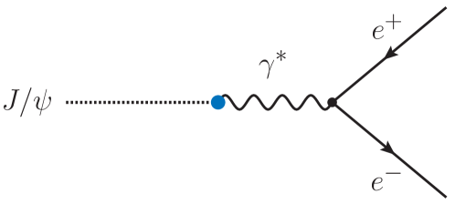
Figure 4: The VMD mechanism of $J/\psi\to e^{+}e^{-}$ decay which determines the $\gamma$-$J/\psi$ coupling.

The $J/\psi$ decay decay constant $f_{\psi}$ can be obtained from the $J/\psi\to e^{+}e^{-}$ decay width, cf. Fig. 4:

$$\Gamma_{J/\psi\to e^{+}e^{-}}=\frac{4\pi\alpha^{2}f^{2}_{\psi}}{3m_{\psi}}.$$ (A.2)

Using recent values Zyla et al. (2020) for $J/\psi$ mass $m_{\psi}=3096.900\pm 0.006$ MeV and electron-positron decay width $\Gamma_{J/\psi\to e^{+}e^{-}}=5.55\pm 0.17$ keV, one finds $f_{\psi}=278\pm 9$ MeV.

The decay widths $\Gamma_{X\to\gamma\gamma}$ and $\Gamma_{X\to J/\psi J/\psi}$ can be obtained via the imaginary part of the $X$-resonance self-energy derived from the following effective interactions

$$\mathcal{L}_{X\gamma\gamma}=-g_{X\gamma\gamma}\phi_{X}F^{\mu\nu}F_{\mu\nu},$$ (A.3)

$$\mathcal{L}_{X\,J/\psi\gamma}=-g_{X\gamma\psi}\phi_{X}G^{\mu\nu}F_{\mu\nu},$$ (A.4)

$$\mathcal{L}_{X\,J/\psi J/\psi}=-g_{X\psi\psi}\phi_{X}G^{\mu\nu}G_{\mu\nu},$$ (A.5)

where $g_{X\gamma\gamma}$, $g_{X\gamma\psi}$ and $g_{X\psi\psi}$ are dimensionful coupling constants, $F_{\mu\nu}=\partial_{\mu}A_{\nu}-\partial_{\nu}A_{\mu}$ is the photon field tensor, and $G_{\mu\nu}=\partial_{\mu}B_{\nu}-\partial_{\nu}B_{\mu}$ is the $J/\psi$ field tensor, $\phi_{X}$ is the scalar field of the $X$-meson. Note that we require gauge-invariance with respect to vector fields, including the massive one. This is where we differ from the recent VMD estimates of Ref. Esposito et al. (2021), which begin from a non-invariant Lagrangian for $J/\psi$. For the pseudoscalar case, one of the field tensors is replaced by its dual, i.e.,

$$F^{\mu\nu} \to\widetilde{F}^{\mu\nu}={\textstyle\frac{1}{2}}\epsilon^{\mu\nu\alpha\beta}F_{\alpha\beta},$$ (A.6)

$$G^{\mu\nu} \to\widetilde{G}^{\mu\nu}={\textstyle\frac{1}{2}}\epsilon^{\mu\nu\alpha\beta}G_{\alpha\beta}.$$ (A.7)

The X-V-V vertex that correspond to each of the Lagrangians (A.3)-(A.5) is

$$V^{\mu\nu}(q_{1},q_{2})=-2ig_{XV_{1}V_{2}}(q_{1}\cdot q_{2}\,g^{\mu\nu}-q_{1}^{\nu}q_{2}^{\mu}).$$ (A.8)

For the pseudoscalar, the vertex reads as:

$$\widetilde{V}^{\mu\nu}(q_{1},q_{2})=2i\widetilde{g}_{XV_{1}V_{2}}\epsilon^{\mu\nu\alpha\beta}q_{1\alpha}q_{2\beta}.$$ (A.9)

Employing the optical theorem, one can write the imaginary part of the self-energy

$$\mathop{\mathrm{Im}}\Pi_{V_{1}V_{2}}(s)=\frac{\lambda^{1/2}(s,m_{1}^{2},m_{2}^{2})}{16\pi s}\sum_{\lambda_{1}\lambda_{2}}\big{|}\mathcal{M}^{\lambda_{1}\lambda_{2}}_{X\to V_{1}V_{2}}\big{|}^{2},$$ (A.10)

where $\lambda_{i}$ are the helicities,

$$\sum_{\lambda_{1}\lambda_{2}}|\mathcal{M}^{\lambda_{1}\lambda_{2}}_{X\to V_{1}V_{2}}|^{2}=\begin{cases}4g^{2}_{XV_{1}V_{2}}\left[2(q_{1}\cdot q_{2})^{2}+q_{1}^{2}q_{2}^{2}\right],\\ 8\widetilde{g}^{2}_{XV_{1}V_{2}}\left[(q_{1}\cdot q_{2})^{2}-q_{1}^{2}q_{2}^{2}\right],\end{cases}$$ (A.11)

and $\lambda(s,m_{1}^{2},m_{2}^{2})=[s-(m_{1}+m_{2})^{2}][s-(m_{1}-m_{2})^{2}]$. Hence, for the scalar and pseudoscalar cases of $X$(6900) we obtain,

$$\mathop{\mathrm{Im}}\Pi_{\gamma\gamma}(s)=\frac{s^{2}}{16\pi}\theta\left(s\right)\times\begin{dcases}g^{2}_{X\gamma\gamma},\\ \widetilde{g}^{2}_{X\gamma\gamma},\end{dcases}$$ (A.12)

$$\mathop{\mathrm{Im}}\Pi_{\gamma J/\psi}(s)=\frac{(s-m_{\psi}^{2})^{3}}{8\pi s}\theta\left(s-m^{2}_{\psi}\right)\times\begin{dcases}g^{2}_{X\gamma\psi},\\ \widetilde{g}^{2}_{X\gamma\psi},\end{dcases}$$ (A.13)

$$\mathop{\mathrm{Im}}\Pi_{J/\psi J/\psi}(s)=\frac{1}{16\pi}\sqrt{1-\frac{4m_{\psi}^{2}}{s}}\theta\left(s-4m^{2}_{\psi}\right)\times\begin{dcases}g^{2}_{X\psi\psi}\big{[}\left(s-2m_{\psi}^{2}\right)^{2}+2m_{\psi}^{4}\big{]},\\ \widetilde{g}^{2}_{X\psi\psi}s\big{(}s-4m_{\psi}^{2}\big{)}.\end{dcases}$$ (A.14)

Assuming $\Gamma_{\mathrm{tot}}=\Gamma_{X\to J/\psi J/\psi}$, one thus obtains the following relations between the decay widths of $X(6900)$ into the $\gamma\gamma$ and di-$J/\psi$ channels:

$$\Gamma_{X\to\gamma\gamma}^{S} = \Gamma_{X\to J/\psi J/\psi}\left(\frac{ef_{\psi}}{m_{\psi}}\right)^{4}\left\{\sqrt{1-\frac{4m_{\psi}^{2}}{m_{X}^{2}}}\left[\left(1-\frac{2m_{\psi}^{2}}{m_{X}^{2}}\right)^{2}+2\left(\frac{m_{\psi}}{m_{X}}\right)^{4}\right]\right\}^{-1},$$ (A.15)

$$\Gamma_{X\to\gamma\gamma}^{PS} = \Gamma_{X\to J/\psi J/\psi}\left(\frac{ef_{\psi}}{m_{\psi}}\right)^{4}\left(1-\frac{4m_{\psi}^{2}}{m_{X}^{2}}\right)^{-\frac{3}{2}}.$$ (A.16)

Applying these relations, we arrive at the estimate of the branching ratios given in Eqs.  (8a) and (8b) with corresponding uncertainties that originate from the parameters entering Eqs. (A.15) and (A.16), i.e. the $X$(6900) and $J/\psi$ masses and $J/\psi$ decay constant.

References

- Aaboud et al. (2017) M. Aaboud et al. (ATLAS), Nature Phys. 13, 852 (2017).
- Sirunyan et al. (2019) A. M. Sirunyan et al. (CMS), Phys. Lett. B 797, 134826 (2019).
- Aad et al. (2021) G. Aad et al. (ATLAS), JHEP 03, 243 (2021).
- LHCb collaboration (2020) LHCb collaboration, Science Bulletin 65, 1983 (2020).
- Richard (2020) J.-M. Richard, Sci. Bull. 65, 1954 (2020).
- Sonnenschein and Weissman (2021) J. Sonnenschein and D. Weissman, Eur. Phys. J. C 81, 25 (2021).
- Faustov et al. (2021) R. N. Faustov, V. O. Galkin, and E. M. Savchenko, Universe 7, 94 (2021).
- Deng et al. (2021) C. Deng, H. Chen, and J. Ping, Phys. Rev. D 103, 014001 (2021).
- Guo and Oller (2021) Z.-H. Guo and J. A. Oller, Phys. Rev. D 103, 034024 (2021).
- Chen et al. (2022) H.-X. Chen, W. Chen, X. Liu, Y.-R. Liu, and S.-L. Zhu, (2022), arXiv:2204.02649 [hep-ph] .
- Karliner and Rosner (2020) M. Karliner and J. L. Rosner, Phys. Rev. D 102, 114039 (2020).
- Debastiani and Navarra (2019) V. R. Debastiani and F. S. Navarra, Chin. Phys. C 43, 013105 (2019).
- Liu et al. (2020) M.-S. Liu, F.-X. Liu, X.-H. Zhong, and Q. Zhao, “Full-heavy tetraquark states and their evidences in the LHCb di- spectrum,” (2020), arXiv:2006.11952 [hep-ph] .
- Lü et al. (2020) Q.-F. Lü, D.-Y. Chen, and Y.-B. Dong, Eur. Phys. J. C 80, 871 (2020).
- Wu et al. (2018) J. Wu, Y.-R. Liu, K. Chen, X. Liu, and S.-L. Zhu, Phys. Rev. D 97, 094015 (2018).
- Bedolla et al. (2020) M. A. Bedolla, J. Ferretti, C. D. Roberts, and E. Santopinto, Eur. Phys. J. C 80, 1004 (2020).
- Wang et al. (2019) G.-J. Wang, L. Meng, and S.-L. Zhu, Phys. Rev. D 100, 096013 (2019).
- Wan and Qiao (2021) B.-D. Wan and C.-F. Qiao, Phys. Lett. B 817, 136339 (2021).
- Liang et al. (2021) Z.-R. Liang, X.-Y. Wu, and D.-L. Yao, Phys. Rev. D 104, 034034 (2021).
- Li et al. (2021) Q. Li, C.-H. Chang, G.-L. Wang, and T. Wang, Phys. Rev. D 104, 014018 (2021).
- Ke et al. (2021) H.-W. Ke, X. Han, X.-H. Liu, and Y.-L. Shi, Eur. Phys. J. C 81, 427 (2021).
- Weng et al. (2021) X.-Z. Weng, X.-L. Chen, W.-Z. Deng, and S.-L. Zhu, Phys. Rev. D 103, 034001 (2021).
- Zhu (2021) R. Zhu, Nucl. Phys. B 966, 115393 (2021).
- Pascalutsa and Vanderhaeghen (2010) V. Pascalutsa and M. Vanderhaeghen, Phys. Rev. Lett. 105, 201603 (2010).
- Pascalutsa (2018) V. Pascalutsa, Causality Rules: A light treatise on dispersion relations and sum rules, IOP Concise Physics (Morgan & Claypool Publishers, 2018).
- Budnev et al. (1975) V. M. Budnev, I. F. Ginzburg, G. V. Meledin, and V. G. Serbo, Phys. Rept. 15, 181 (1975).
- Pascalutsa et al. (2012) V. Pascalutsa, V. Pauk, and M. Vanderhaeghen, Phys. Rev. D 85, 116001 (2012).
- Harland-Lang et al. (2019) L. A. Harland-Lang, V. A. Khoze, and M. G. Ryskin, The European Physical Journal C 79 (2019), 10.1140/epjc/s10052-018-6530-5.
- Harland-Lang et al. (2016) L. A. Harland-Lang, V. A. Khoze, and M. G. Ryskin, The European Physical Journal C 76 (2016), 10.1140/epjc/s10052-015-3832-8.
- Wang et al. (2018) J. Z. Wang, Z. F. Sun, X. Liu, and T. Matsuki, European Physical Journal C 78, 1 (2018).
- Bern et al. (2001) Z. Bern, A. De Freitas, L. J. Dixon, A. Ghinculov, and H. L. Wong, JHEP 11, 031 (2001).
- Kłusek-Gawenda et al. (2016) M. Kłusek-Gawenda, W. Schäfer, and A. Szczurek, Phys. Lett. B 761, 399 (2016).
- Krintiras et al. (2022) G. K. Krintiras, I. Grabowska-Bold, M. Kłusek-Gawenda, E. Chapon, R. Chudasama, and R. Granier de Cassagnac, (2022), arXiv:2204.02845 [hep-ph] .
- Barnea et al. (2006) N. Barnea, J. Vijande, and A. Valcarce, Phys. Rev. D 73, 054004 (2006).
- Berezhnoy et al. (2012) A. V. Berezhnoy, A. V. Luchinsky, and A. A. Novoselov, Phys. Rev. D 86, 034004 (2012).
- Karliner et al. (2017) M. Karliner, S. Nussinov, and J. L. Rosner, Phys. Rev. D 95, 034011 (2017).
- Wang (2017) Z.-G. Wang, Eur. Phys. J. C 77, 432 (2017).
- Liu et al. (2019) M.-S. Liu, Q.-F. Lü, X.-H. Zhong, and Q. Zhao, Phys. Rev. D 100, 016006 (2019).
- Lundhammar and Ohlsson (2020) P. Lundhammar and T. Ohlsson, Phys. Rev. D 102, 054018 (2020).
- Barger and Phillips (1975) V. Barger and R. Phillips, Physics Letters B 58, 433 (1975).
- Redlich et al. (2000) K. Redlich, H. Satz, and G. M. Zinovjev, Eur. Phys. J. C 17, 461 (2000).
- Zyla et al. (2020) P. A. Zyla et al. (Particle Data Group), PTEP 2020, 083C01 (2020).
- Esposito et al. (2021) A. Esposito, C. A. Manzari, A. Pilloni, and A. D. Polosa, Phys. Rev. D 104, 114029 (2021).