Heat transport in an optical lattice via Markovian feedback control

Abstract

Ultracold atoms offer a unique opportunity to study many-body physics in a clean and well-controlled environment. However, the isolated nature of quantum gases makes it difficult to study transport properties of the system, which are among the key observables in condensed matter physics. In this work, we employ Markovian feedback control to synthesize two effective thermal baths that couple to the boundaries of a one-dimensional Bose-Hubbard chain. This allows for the realization of a heat-current-carrying state. We investigate the steady-state heat current, including its scaling with system size and its response to disorder. In order to study large systems, we use semi-classical Monte-Carlo simulation and kinetic theory. The numerical results from both approaches show, as expected, that for non- and weakly interacting systems with and without disorder one finds the same scaling of the heat current with respect to the system size as it is found for systems coupled to thermal baths. Finally, we propose and test a scheme for measuring the energy flow. Thus, we provide a route for the quantum simulation of heat-current-carrying steady states of matter in atomic quantum gases.

I Introduction

Transport plays a crucial role in understanding states of matter in and out of equilibrium. The study of transport properties in real materials is always influenced by the effect of impurities, lattice defects and phonons. Ultracold atoms, in turn, offer to study transport also in systems, which are isolated from their environment and free of impurities or disorder, unless these properties are engineered on purpose in a controlled fashion. Moreover, they are highly tunable and can be manipulated and probed on their (large) intrinsic time and lengths scales RevModPhys.80.885 . This makes them promising quantum simulators also for transport. However, the isolated nature of quantum gases prevents a direct connection of the system, e.g., to leads or extended thermal baths of different temperature. To investigate the transport properties of quantum gases, a variety of approaches have been exploited. For instance, particle transport has been investigated by observing the response of the system to variations of the external potential via measuring the density distribution PhysRevLett.122.153602 ; Brown2019 , the quasimomentum distribution Pasienski2010 ; PhysRevLett.114.083002 , monitoring the center of mass motion PhysRevLett.92.160601 ; PhysRevLett.93.120401 ; PhysRevLett.94.120403 ; PhysRevLett.99.220601 , and expansion dynamics PhysRevLett.95.170409 ; PhysRevLett.95.170410 ; PhysRevLett.104.220602 ; Roati2008 ; Billy2008 ; Deissler2010 ; Kondov2011 ; Jendrzejewski2012 ; Choi2016 ; PhysRevLett.110.205301 ; Schneider2012 , or by studying mass flow through optically structured mesoscopic devices Krinner2015 ; Krinner2016 ; Krinner_2017 ; PhysRevX.8.011053 . Spin transport was studied by introducing spin inhomogeneities followed by monitoring the spin evolution sommer2011universal ; Fukuhara2013 ; Valtolina2017 ; Nichols2019 or investigating the decoherence of spin texture Koschorreck2013 ; PhysRevLett.113.147205 ; PhysRevLett.118.130405 ; Bardon2014 ; PhysRevLett.114.015301 ; Jepsen2020 . And heat transport was investigated by locally heating the system, after which the equilibration is studied by monitoring the temperature bias PhysRevLett.103.095301 or particle imbalance Brantut2013 ; PhysRevX.11.021034 . However, in all these experiments, transport occurs as a transient phenomenon only.

In this work, we employ Markovian feedback control PhysRevA.49.2133 to engineer two effective thermal baths that are coupled to a one-dimensional Bose-Hubbard chain. This allows for the realization of a heat-current-carrying steady state. As a measurement-based approach, Markovian feedback control continuously adds a signal-proportional feedback term to the system Hamiltonian. The dynamics of the system is then described by a feedback-modified Lindblad master equation (ME) PhysRevA.49.2133 . By properly choosing the measurement and feedback operators, the system dynamics can be steered towards a desired target state. The Markovian feedback method has been applied to various control problems, including the stabilization of arbitrary one-qubit quantum states PhysRevA.64.063810 ; PhysRevLett.117.060502 , the manipulation of quantum entanglement between two qubits PhysRevA.71.042309 ; PhysRevA.76.010301 ; PhysRevA.78.012334 ; Wang2010 as well as optical and spin squeezing PhysRevA.50.4253 ; PhysRevA.65.061801 ; 2021arXiv210202719B . In our previous works, we have shown that Markovian feedback control can be used to cool a bosonic quantum gas in an optical lattice wu2021cooling and to engineer a thermal bath wu2022FiniteT . Here, we will generalize such a feedback scheme to engineer two thermal baths at the boundaries of an optical lattice and study the heat transport through the chain induced by it. Different from our previous works wu2021cooling ; wu2022FiniteT , this requires to work out a scheme for engineering artificial thermal baths by employing local measurements and feedback on a few lattice sites only.

The paper is organized as follows: in Section II, we introduce our model and some basics of Markovian feedback control. This is followed by the description of a two-site feedback scheme in Section III, which can be used to engineer a finite-temperature bath. In Section IV, we study the steady-state heat current of the system, including its scaling behavior with system size (see Section IV.3) and its response to disorder (see Section IV.4). The experimental implementation of our scheme is discussed in Section V, including the measurement of heat current by measuring single-particle density matrix. A summary of the main results is presented in Section VI to conclude.

II Model and Markovian feedback scheme

The system under consideration is a one-dimensional optical lattice with $N$ interacting bosonic atoms, which can be described by the Bose-Hubbard model,

$$H=-J\sum\limits_{l=1}^{M-1}(a_{l}^{\dagger}a_{l+1}+a_{l+1}^{\dagger}a_{l})+\frac{U}{2}\sum\limits_{l=1}^{M}n_{l}(n_{l}-1)+\sum\limits_{l=1}^{M}{V_{l}n_{l}},$$ (1)

where $a_{l}$ annihilates a particle on site $l$ and $n_{l}=a_{l}^{\dagger}a_{l}$ counts the particle number on site $l$, with $\sum\nolimits_{l}n_{l}=N$. The first term in (1) describes tunneling between neighboring sites with rate $J$, the second term denotes on-site interactions with strength $U$ and the last term describes an on-site potential. In the following discussion, $V_{l}=0$ unless stated otherwise.

Let us consider a homodyne measurement of an operator $c$. The dynamical evolution of the system is then described by the stochastic master equation (SME) wiseman2009quantum  ($\hbar=1$ hereafter),

$$d\rho_{c}=-i[H,\rho_{c}]dt+{\cal D}[c]\rho_{c}dt+{\cal H}[c]\rho_{c}dW,$$

with ${\cal H}[c]\rho:=c\rho+\rho c^{\dagger}-{\rm Tr}[(c+c^{\dagger})\rho]\rho$ and ${\cal D}[c]\rho:=c\rho c^{\dagger}-\frac{1}{2}(c^{\dagger}c\rho+\rho c^{\dagger}c)$. Here $\rho_{c}$ denotes the quantum state conditioned on the measurement result, $I_{\rm hom}={\rm Tr}[(c+c^{\dagger})\rho]+\xi(t)$, with $\xi(t)=dW/dt$ and $dW$ being the standard Wiener increment with mean zero and variance $dt$. The quantum backaction of a weak measurement can be used for tailoring the system’s dynamics and to prepare target states. While the state generated in this way is conditional due to the nondeterministic nature of measurement, the introduction of feedback using the information acquired from the measurements allows to steer the system’s dynamics into a desired state.

Here we consider a direct feedback strategy, where a signal-dependent, i.e. conditional, feedback term $I_{\rm hom}F$ is added to the Hamiltonian. According to the theory of Markovian feedback control PhysRevA.49.2133 , the system is then governed by the feedback-modified SME

$$d\rho_{c} = -i[H+H_{\rm fb},\rho_{c}]dt+{\cal D}[A]\rho_{c}dt+{\cal H}[A]\rho_{c}dW,$$

with operators

$$A=c-iF,\quad H_{\rm fb}=\frac{1}{2}(c^{\dagger}F+Fc).$$ (2)

By taking the ensemble average of the possible measurement outcomes, we arrive at the feedback-modified ME PhysRevA.49.2133

$$\dot{\rho}=-i[H+H_{\rm fb},\rho]+{\cal D}[A]\rho.$$ (3)

The effect induced by the feedback loop is seen to replace the collapse operator $c$ by $A$ and to add an extra term $H_{\rm fb}$ to the Hamiltonian. The latter is proportional to measurement strength and thus can be safely neglected for weak measurements.

III Two-site feedback scheme

Before approaching the scenario relevant for heat transport, where the feedback is mimicking two thermal baths of different temperature at both ends of the system, let us first investigate how the local coupling to a single bath can be realized. Previously, we considered already the engineering of a thermal bath using measurement and feedback operators acting globally on all sites of a lattice wu2022FiniteT . In contrast, we now consider the following two-site measurement and feedback operator

$$c_{l} =\sqrt{\gamma}(x_{l}n_{l}-{x_{l}^{-1}}n_{l+1}),\quad F_{l} =-i\lambda\sqrt{\gamma}(a_{l}^{\dagger}a_{l+1}-a_{l+1}^{\dagger}a_{l}),$$ (4)

where $\gamma$ is the measurement strength, $\lambda$ is a free parameter to be determined, $x_{l}=g_{l+1}/g_{l}$ and $g_{l}$ are the coefficients of the single-particle ground state, i.e., $|g\rangle=\sum\nolimits_{l}{g_{l}|l\rangle}$. The feedback-modified collapse operator then reads

$$A_{l}=c_{l}-iF_{l}.$$ (5)

Note that the sites $l$ and $l+1$ where to perform the measurement and feedback can be any neighboring two sites on the lattice.

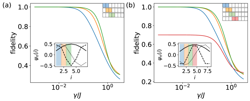
Figure 1: The fidelity (6) between the steady state of the ME (3) for our two-site feedback scheme (4) and the ground state of the system (1) as a function of the measurement strength $\gamma$ for two different lattice sizes with $N=2$ non-interacting particles: (a) $M=7$ and (b) $M=8$. Different colored curves correspond to schemes performing at different sites as indicated by the sketch at the upper right corner with the corresponding colors. As expected, for weak measurements $\gamma\ll J$, the fidelity approaches $1$. The only case where the feedback-controlled system does not settle down to the ground state [see the red curve in (b)] for weak measurements is due to the fact that the ground state is not the unique dark state of the collapse operator. From the inset, which shows the first three eigenstates of the system, one can see that the first excited state for $M=8$ in (b) as denoted by the dashed line has the same wavefunction values as the ground state (see solid line) at the feedback-controlled sites (site $4$ and site $5$), and thus is also a dark state of the collapse operator.

For $N$ non-interacting particles, with $\lambda=1$, one can show that $A_{l}|g\rangle^{\otimes N}=0$, where $|g\rangle^{\otimes N}$ denotes the ground state of the system, with all particles occupying the single-particle ground state, $|{g}\rangle$. It is easy to check it for the single-particle problem, where the collapse operator reduces to

$$A_{l}=\frac{g_{l+1}}{g_{l}}{|l\rangle\langle l|}-\frac{g_{l}}{g_{l+1}}{|l+1\rangle\langle l+1|}-(|l\rangle\langle l+1|-|l+1\rangle\langle l|).$$

Applying it to the ground state $|g\rangle$, one gets

$$A_{l}|g\rangle=g_{l+1}|l\rangle-g_{l}|l+1\rangle-g_{l+1}|l\rangle+g_{l}|l+1\rangle=0.$$

When there are no interactions between the particles, the multi-particle problem is equivalent to the single-particle problem. Namely, the ground state of the system is a dark state of the collapse operator $A_{l}$. Assuming weak measurements with strength $\gamma\ll J$, where the impact of the additional term in the Hamiltonian $H_{\rm bf}\propto\gamma$ is negligible, the dissipative dynamics will then drive the system towards the ground state (if it is the unique dark state of the collapse operator).

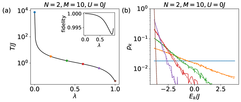
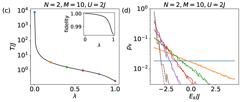
Figure 2: Engieering a finite-temperature bath using two-site feedback scheme (4). (a, c) The effective temperature of the feedback-synthesized bath as a function of the feedback strength $\lambda$. The inset shows the fidelity between the steady state and the corresponding effective thermal state. (b, d) The distribution of the steady state on the eigenbasis for various $\lambda$ marked in (a, c). $k$ is the label of the $k$th eigenstate, with energy in ascending order. Dashed lines are the corresponding thermal distributions. Parameters are $V_{l}=0$, $\gamma=0.01J$.

In Fig. 1, we show the fidelity between the steady state of the ME (3) for our two-site feedback scheme (4), $\rho_{\rm ss}$, and the ground state of the system (1), $|G\rangle$, i.e.,

$$f=\sqrt{\langle G|\rho_{\rm ss}|G\rangle},$$ (6)

as a function of the measurement strength $\gamma$ for two different lattice sizes with $N=2$ non-interacting particles: (a) $M=7$ and (b) $M=8$. Different colored curves correspond to schemes performing at different sites as indicated by the sketch at the upper right corner with the corresponding colors. As expected, for weak measurements $\gamma\ll J$, the fidelity approaches $1$. The only case where the feedback-controlled system does not settle down to the ground state [see the red curve in (b)] for weak measurements is due to the fact that the ground state is not the unique dark state of the collapse operator. Namely, from the inset, which shows the first three eigenstates of the system, one can see that the first excited state for $M=8$ in (b) as denoted by the dashed line has the same wavefunction values as the ground state (see solid line) at the feedback-controlled sites (site $4$ and site $5$), and thus is also a dark state of the collapse operator.

For $0<\lambda<1$, the proposed scheme can be used to engineer a finite-temperature bath. In Fig. 2, we show the effective temperature of the feedback-synthesized bath as a function of the feedback strength $\lambda$ for (a) non-interacting and (c) interacting systems. The inset shows the fidelity between the steady state and the corresponding effective thermal state, which is close to $1$ over the whole parameter regime. As a second measure, we compare the probability distribution in the eigenstate basis for the steady states at various $\lambda$ (solid lines) marked in Fig. 2(a, c) to the corresponding thermal states (dashed lines) in Fig. 2(b, d). They are found to agree with each other very well.

IV Heat transport

IV.1 Model

We use the two-site feedback scheme to heat up the system on one side and cool it down on the other side, see the sketch in Fig. 3. Note that the feedback-controlled sites for the bath on the right hand side of the chain are chosen differently from the left hand site, not to be the outermost sites, otherwise the system will be effectively coupled to one thermal bath at the average temperature of the two synthesized baths PhysRevE.92.062119 . The two measurement operations are assumed to be independent of each other (see Section V for the experimental implementation), giving rise to uncorrelated signals. The dynamics of the system is described by the feedback master equation,

$$\dot{\rho}={\cal L}\rho=-i[H,\rho]+{\cal L}_{L}\rho+{\cal L}_{R}\rho,$$ (7)

where

$${\cal L}_{\mu}\rho=-i[H_{{\rm fb}}^{\mu},\rho]+{\cal D}[A_{\mu}](\rho),\quad(\mu=L,R)$$ (8)

describes the impact of the feedback control on the $\mu$ side of the chain with $H_{{\rm fb}}^{L}\equiv H_{{\rm fb}}^{(1)}$, $H_{{\rm fb}}^{R}\equiv H_{{\rm fb}}^{(M-2)}$, $H_{\rm fb}^{(l)}=(c_{l}F_{l}+F_{l}c_{l})/2$ and

$$A_{L}\equiv A_{1}=c_{1}-i\lambda_{L}F_{1},\quad A_{R}\equiv A_{M-2}=c_{M-2}-i\lambda_{R}F_{M-2}.$$ (9)

Cooling is realized by setting $\lambda=1$, corresonding to a zero-temperature bath, and heating by setting $0<\lambda<1$, corresponding to finite positive temperatures.

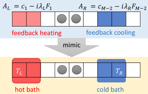
Figure 3: A sketch of our feedback scheme for realizing a heat-current-carrying state. A one-dimensional optical lattice is cooled and heated at both ends via feedback control, as shown in the upper panel in blue background. This mimics the effect of coupling the system locally to a hot bath and a cold bath (see lower panel in yellow background), and thus allows us to study the heat transport property of the system.

IV.2 Heat current

The steady state of the system is a heat-current-carrying state. The heat current ${\cal J}$ is calculated from the continuity equation for energy,

$$\frac{d\langle H\rangle}{dt}={\cal J}_{L}+{\cal J}_{R}.$$ (10)

It follows from the ME (7) that

$$\frac{d\langle H\rangle}{dt}={\rm Tr}\left\{H{\cal L}_{L}\rho\right\}+{\rm Tr}\left\{H{\cal L}_{R}\rho\right\}.$$

So we have

$${\cal J}_{L}={\rm Tr}\left\{H{\cal L}_{L}\rho\right\},\quad{\cal J}_{R}={\rm Tr}\left\{H{\cal L}_{R}\rho\right\}.$$ (11)

In the steady state, $d\langle H\rangle/dt=0$. Thus, the steady-state heat current is

$${\cal J}_{\rm ss}={\cal J}_{L}=-{\cal J}_{R}={\rm Tr}\left\{H{\cal L}_{L}\rho_{\rm ss}\right\}=-{\rm Tr}\left\{H{\cal L}_{R}\rho_{\rm ss}\right\}.$$ (12)

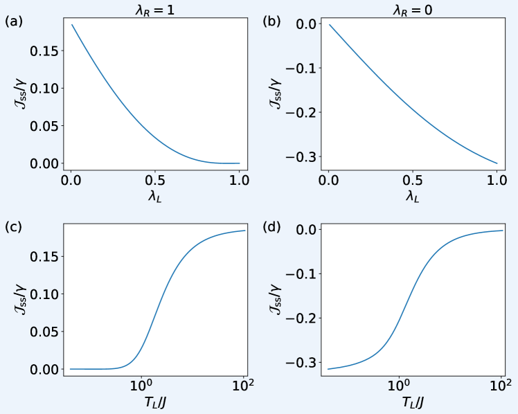
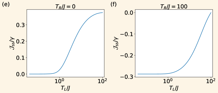
Figure 4: The panels in blue background (a-d) are the results for our scheme. The steady-state heat current is shown as a function of (a, b) the feedback strength $\lambda_{L}$ and (c, d) the effective temperature $T_{L}$ of the left bath. For the right bath, (a, c) $\lambda_{R}=1$, which corresponds to a zero-temperature bath; (b, d) $\lambda_{R}=0$, which corresponds to an infinite-temperature bath. In both cases, the heat current increases with the temperature imbalance between the two baths. Similar behavior is observed when the system is coupled to real thermal bath, as shown in the panels (e, f) in yellow background. Parameters are $N=1$, $M=10$, $V_{l}=0$, $\gamma=0.01J$.

Figure 4 shows the steady-state heat current of a system with $N=1$ particle in a lattice with $M=10$ sites as a function of the feedback strength $\lambda_{L}$ [see (a) and (b)] and the effective temperature $T_{L}$ [see (c) and (d)] of the left bath. For the right bath, in (a, c) $\lambda_{R}=1$, which corresponds to a zero-temperature bath ($T_{R}=0$); in (b, d) $\lambda_{R}=0$, which corresponds to an infinite-temperature bath ($T_{R}=\infty$). As expected, the heat current in both cases increases with the temperature imbalance between the two baths. Similar behavior is observed when the system is coupled to real thermal bath, as shown in Fig. 4(e, f). Since the heat current in non-equilibrium is not solely determined by the temperature of the baths, we do not expect exactly the same behavior for our scheme and the thermal bath case. In the following discussion, we will focus on the case with $\lambda_{R}=1$ for our scheme.

IV.3 System-size scaling

We are interested in the scaling of the steady-state heat current with system size. To study this property, we have to deal with large systems, which are not accessible by exact diagonalization. For a system with $N$ particles and $M$ sites, the dimension of the Hilbert space is $D=(N+M-1)!/N!/(M-1)!$, which means the Liouvillian superoperator ${\cal L}$ is a $D^{2}$ by $D^{2}$ matrix. For instance, for $M=4$ and $N=8$, $D=330$, the Liouvillian superoperator will be a $108900$ by $108900$ matrix. This simple example shows that it is hard to treat large systems by using the exact diagonalization approach. In order to circumvent this problem, we resort to two different approaches: kinetic theory and semi-classical Monte Carlo simulation, as described in the following.

For the non-interacting case, the system Hamiltonian reads

$$H=\sum\limits_{k}{\epsilon_{k}n_{k}},$$

with single-particle eigenenergy $\epsilon_{k}=-2J\cos{\frac{k\pi}{M+1}}$ in the absence of on-site potential. Here $n_{k}=c_{k}^{\dagger}c_{k}$ counts the number of particles in the single-particle eigenstate $|k\rangle$, with $c_{k}^{\dagger}=\sum\nolimits_{l}\langle l|k\rangle a_{l}^{\dagger}$ being the corresponding creation operator. The continuity equation for energy then reads

$$\frac{d\langle H\rangle}{dt}=\sum\nolimits_{k}\epsilon_{k}\langle\dot{n}_{k}\rangle.$$ (13)

It depends on the time evolution of the mean occupations $\langle n_{k}\rangle$, which is governed by

$$\langle\dot{n}_{k}\rangle=\sum\nolimits_{q}\left[R_{kq}\langle n_{q}(1+n_{k})\rangle-R_{qk}\langle n_{k}(1+n_{q})\rangle\right],$$ (14)

with $R_{kq}=R_{kq}^{L}+R_{kq}^{R}=|\langle k|A_{L}|q\rangle|^{2}+|\langle k|A_{R}|q\rangle|^{2}$ being the single-particle transfer rate from single-particle eigenstate $q$ to $k$. The steady-state heat current is given by

$${\cal J}_{\rm ss}={\cal J}_{L}=\sum\nolimits_{k}\epsilon_{k}\langle\dot{n}_{k}\rangle_{L}=-{\cal J}_{R}=-\sum\nolimits_{k}\epsilon_{k}\langle\dot{n}_{k}\rangle_{R}$$ (15)

with

$$\langle\dot{n}_{k}\rangle_{\mu}=\sum\nolimits_{q}\left[R_{kq}^{\mu}\langle n_{q}(1+n_{k})\rangle_{\rm ss}-R_{qk}^{\mu}\langle n_{k}(1+n_{q})\rangle_{\rm ss}\right],\quad(\mu=L,R).$$ (16)

Here the subscript ‘ss’ of the expectation values denotes the steady-state expectation values, which satisfy

$$\sum\nolimits_{q}\left[R_{kq}\langle n_{q}(1+n_{k})\rangle_{\rm ss}-R_{qk}\langle n_{k}(1+n_{q})\rangle_{\rm ss}\right]=0.$$ (17)

In the following, we describe two approaches to calculate the steady-state expectation values approximately.

IV.3.1 Semi-classical Monte Carlo simulation.

In the semi-classical Monte-Carlo simulation PhysRevE.92.062119 , the density matrix is approximated by a mixed superposition of Fock states with respect to single-particle eigenstates $\rho=\sum\nolimits_{\bf n}{p_{\bf n}|{\bf n}\rangle\langle{\bf n}|}$, with ${\bf n}=(n_{1},n_{2},\ldots,n_{M})$, i.e., the off-diagonal elements which decouple with the diagonal elements and decay with time are neglected for weak system-bath coupling BRE02 . The equations of motion for the Fock-space occupation probabilities $p_{\bf n}$ are then mapped to a random walk in the classical space spanned by the Fock states $|{\bf n}\rangle$ (but not their superpositions). We perform these simulations by using the Gillespie-type algorithm described in Ref. PhysRevE.92.062119 . By averaging over the long-time dynamics of many trajectories, we can then compute steady-state expectation values, $\langle{n}_{k}\rangle_{\rm ss},\langle{n}_{k}{n}_{q}\rangle_{\rm ss}$, etc. The steady-state heat current is then calculated by using Eq. (15). This approach gives accurate results after sufficient statistical sampling. For a given accuracy, the sampling size increases with increasing system sizes.

IV.3.2 Kinetic theory.

We use kinetic theory to treat large systems where the semi-classical Monte Carlo simulation is computationally expensive. The set of equations (14) is not closed as the single-particle correlations depend on two-particle correlations, which in turn depend on three-particle correlations, and so on. To get a closed set of equations, we employ the mean-field approximation $\langle n_{k}n_{q}\rangle\approx\langle n_{k}\rangle\langle n_{q}\rangle$, which then leads to

$$\langle\dot{n}_{k}\rangle\approx\sum\nolimits_{q}\left\{R_{kq}\langle n_{q}\rangle[1+\langle n_{k}\rangle]-R_{qk}\langle n_{k}\rangle[1+\langle n_{q}\rangle]\right\}.$$

The steady-state heat current is calculated approximately by using Eq. (15) with

$$\langle\dot{n}_{k}\rangle_{L}\approx\sum\limits_{q}\left\{R_{kq}^{L}\langle n_{q}\rangle_{\rm ss}[1+\langle n_{k}\rangle_{\rm ss}]-R_{qk}^{L}\langle n_{k}\rangle_{\rm ss}[1+\langle n_{q}\rangle_{\rm ss}]\right\},$$ (18)

where the steady-state expectation values are obtained by solving $\langle\dot{n}_{k}\rangle=0$, i.e.,

$$\sum\limits_{q}\left\{R_{kq}\langle n_{q}\rangle_{\rm ss}[1+\langle n_{k}\rangle_{\rm ss}]-R_{qk}\langle n_{k}\rangle_{\rm ss}[1+\langle n_{q}\rangle_{\rm ss}]\right\}=0.$$ (19)

IV.3.3 Results.

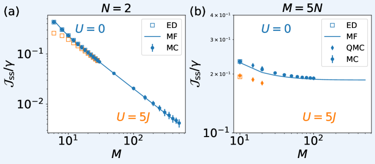
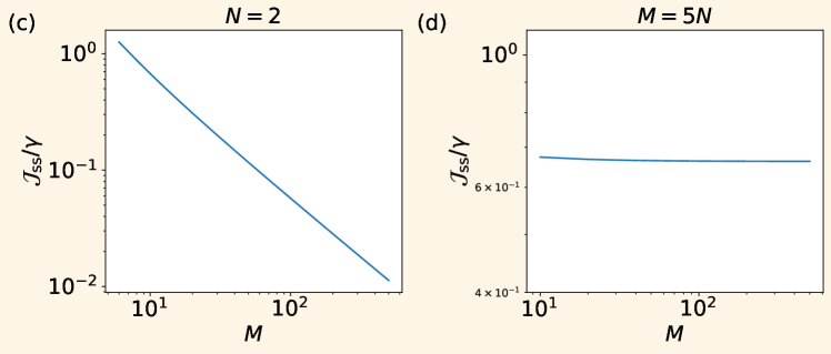
Figure 5: System-size scaling of the steady-state heat current for (a, c) a fixed particle number $N=2$ and (b, d) a fixed filling factor $n=N/M=1/5$. The panels in blue background (a, b) are the results for our scheme. The panels in yellow background (c, d) are the results when the system is coupled to thermal bath. The blue (orange) data denote the results for the non-interacting (interacting) case. The squares denote the results from exact diagonalization (ED). The diamonds denote the results from quantum jump Monte-Carlo simulations (QMC). The bullets denote the results from semi-classical Monte Carlo (MC) simulation. The solid lines are the results from kinetic theory with mean-field (MF) approximation. For the MC simulation, the results are obtained by averaging over the long-time [up to $\gamma t=10^{5}$ for (a) and $\gamma t=10^{6}$ for (b)] dynamics of $100$ trajectories. The error bar denotes one standard deviation. Parameters are $V_{l}=0$, $\gamma=0.01J$, $\lambda_{L}=0.2$, $\lambda_{R}=1$, $T_{L}=10J$, $T_{R}=0.01J$.

Figure 5 shows the system-size dependence of the steady-state heat current. Let us first focus on the non-interacting case, as shown by the blue data. For a fixed particle number $N=2$ [see Fig. 5(a)], the results from the three approaches, i.e., exact diagonalization (squares), Monte Carlo simulation (bullets), and mean-field approximation (solid lines), agree with each other. The steady-state heat current is found to decrease with the lattice size $M$ as $M^{-1}$, like for diffusive transport 2021arXiv210414350L . For a fixed filling factor at $N/M=1/5$ [see Fig. 5(b)], a slight deviation is found between the mean-field results and the Monte Carlo results. Nevertheless, the results from both approaches show that in this case the current first decreases with system size, but then saturates to a finite value, independent of the lattice size $M$, corresponding to ballistic transport 2021arXiv210414350L . These results are consistent with that when the system is coupled to two thermal baths on its ends, as shown in Fig. 5(c) and (d).

Now let us turn on interactions. For a fixed particle number, which can be calculated by using exact diagonalization [the orange squares in Fig. 5(a)], the interactions are found to have some impact on the steady-state heat current for small systems. While this effect becomes weaker with increasing system sizes, and thus does not change the scaling of the current with system size. For a fixed filling factor, the numerical simulation is challenging. We resort to quantum jump Monte Carlo method PhysRevLett.68.580 ; Daley2014Review , which offers an efficient stochastic simulation of the master equation by means of quantum trajectories. We are able to calculate the heat current of the interacting system for up to $20$ lattice sites [see orange diamonds in Fig. 5(b)]. We can clearly observe that it is reduced with respect to the heat current for the non-interacting system. Moreover, we can see that it drops with $M$. The accessible system sizes of $20$ do, however, not allow to reach the regime, where the ballistic transport of the non-interacting system becomes apparent from the saturation of the heat current. While it would have been interesting to study numerically, whether/how ballistic transport breaks down with increasing interactions, we would like to point out that our scheme opens the opportunity to investigate this question experimentally in a quantum simulation, where heat-current-carrying states also of larger interacting systems are prepared using feedback control.

IV.4 Influence of disorder

Here we investigate the influence of disorder on the steady-state heat current. For this purpose, we add a random on-site potential, with $V_{l}$ being a random number uniformly distributed in the range $[-V_{d},V_{d}]$ . The results are shown in Fig. 6, which are averaged over $100$ trajectories with different disorder configurations. As expected, the current decreases with the disorder strength $V_{d}$, as shown in Fig. 6(a). Figure 6(b) shows the current as a function of the lattice site number $M$ at $V_{d}=0.2J$ and fixed filling $N/M=1/5$. The decay of the current with increasing system size is approximately exponential, as indicated by the close-to-linear form of the current in the log-$y$ plot. Similar behaviors are observed when the system is coupled to real thermal baths, as shown in Fig. 6(c) and (d).

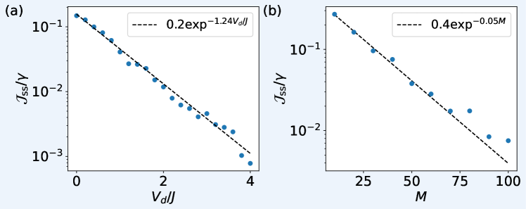
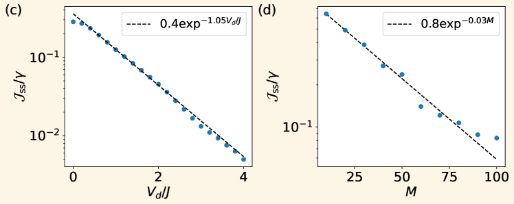
Figure 6: (a, c) The steady-state heat current ${\cal J}_{\rm ss}$ as a function of the disorder strength for one particle on $M=10$ sites. The results are obtained from exact diagonalization. (b, d) The system-size scaling of ${\cal J}_{\rm ss}$ at $V_{d}=0.2J$ for $N=M/5$. The results are obtained from kinetic theory with mean-field approximation. The panels in blue background (a, b) are the results for our scheme. The panels in yellow background (c, d) are the results when the system is coupled to thermal bath. All the results are averaged over $100$ trajectories with different disorder configurations. Parameters are $U=0$, $\gamma=0.01J$, $\lambda_{L}=0.1$, $\lambda_{R}=1$, $T_{L}=10J$, and $T_{R}=0.01J$.

V Experimental Implementation

Now we discuss the experimental implementation of our scheme. For the engineering of the local baths, one needs to perform measurements of the on-site population, and add the corresponding feedback control. The former can be implemented via homodyne detection of the off-resonant scattering of structured probe light from the atoms PhysRevLett.114.113604 ; PhysRevLett.115.095301 ; RevModPhys.85.553 . To engineer two independent baths, one can for instance use two probe beams with different frequencies. The feedback control of tunneling with complex rate can be realized by modulating the on-site energy of the relevant sites (see Appendix A).

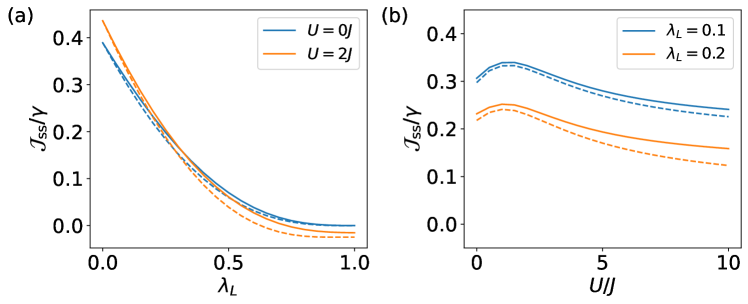
Figure 7: The steady-state heat current ${\cal J}_{\rm ss}$ as a function of (a) the feedback strength $\lambda_{L}$ for two different interaction strengths $U$, and (b) the interaction strength $U$ for two different feedback strength $\lambda_{L}$. Parameters are $N=2$, $M=10$, $V_{l}=0$, $\gamma=0.01J$, and $\lambda_{R}=1$. The solid lines are exact results. The dashed lines are the approximated results by using Wick’s decomposition, Eqs.(21)-(24).

For the heat current, we propose to make use of the measurement of single-particle density matrices $\langle a_{i}^{\dagger}a_{j}\rangle$, which is experimentally accessible PhysRevLett.121.260401 . It can be shown that the heat current is given by

$$\frac{{\cal J}_{L}}{\gamma} =\frac{J}{2}[(x+x^{-1})^{2}+4\lambda_{L}^{2}]\langle a_{1}^{\dagger}a_{2}+a_{2}^{\dagger}a_{1}\rangle+\frac{J}{2}(\lambda_{L}^{2}+x^{-2})\langle a_{2}^{\dagger}a_{3}+a_{3}^{\dagger}a_{2}\rangle$$ (20)

$$+J\lambda_{L}(x+x^{-1})\langle(a_{1}^{\dagger}a_{2}-a_{2}^{\dagger}a_{1})^{2}\rangle-2J\lambda_{L}\langle(n_{1}-n_{2})(xn_{1}-x^{-1}n_{2})\rangle$$

$$-\frac{J\lambda_{L}}{2}\langle(a_{1}^{\dagger}a_{3}+a_{3}^{\dagger}a_{1})(xn_{1}-x^{-1}n_{2})+{\rm h.c.}\rangle$$

$$-\frac{J\lambda_{L}}{2x}\langle(a_{1}^{\dagger}a_{2}-a_{2}^{\dagger}a_{1})(a_{2}^{\dagger}a_{3}-a_{3}^{\dagger}a_{2})+{\rm h.c.}\rangle$$

$$-\frac{U\lambda_{L}}{4}\langle(xn_{1}-x^{-1}n_{2})(n_{1}-n_{2})(a_{1}^{\dagger}a_{2}+a_{2}^{\dagger}a_{1})+{\rm h.c.}\rangle$$

$$-\frac{U\lambda_{L}}{4}\langle(n_{1}-n_{2})(a_{1}^{\dagger}a_{2}+a_{2}^{\dagger}a_{1})(xn_{1}-x^{-1}n_{2})+{\rm h.c.}\rangle$$

$$-U\lambda_{L}^{2}(\langle(n_{1}-n_{2})^{2}\rangle-\langle(a_{1}^{\dagger}a_{2}+a_{2}^{\dagger}a_{1})^{2}\rangle).$$

By using Wick’s theorem, corresponding to the mean-field approximation used already for the kinetic theory,

$$\langle a_{k}^{\dagger}a_{q}a_{p}^{\dagger}a_{l}\rangle\approx\langle a_{k}^{\dagger}a_{q}\rangle\langle a_{p}^{\dagger}a_{l}\rangle+\langle a_{k}^{\dagger}a_{l}\rangle\langle a_{q}a_{p}^{\dagger}\rangle,$$

we have

$$\langle(a_{1}^{\dagger}a_{2}-a_{2}^{\dagger}a_{1})^{2}\rangle \approx\langle a_{1}^{\dagger}a_{2}-a_{2}^{\dagger}a_{1}\rangle^{2}+\langle a_{1}^{\dagger}a_{2}\rangle^{2}+\langle a_{2}^{\dagger}a_{1}\rangle^{2}-2\langle n_{1}\rangle\langle n_{2}\rangle-\langle n_{1}\rangle-\langle n_{2}\rangle,$$ (21)

$$\langle(n_{1}-n_{2})(xn_{1}-x^{-1}n_{2})\rangle$$ (22)

$$\approx x\langle n_{1}\rangle(2\langle n_{1}\rangle-\langle n_{2}\rangle+1)+x^{-1}\langle n_{2}\rangle(2\langle n_{2}\rangle-\langle n_{1}\rangle+1)-(x+x^{-1})|\langle a_{1}^{\dagger}a_{2}\rangle|^{2},$$

$$\langle(a_{1}^{\dagger}a_{3}+a_{3}^{\dagger}a_{1})(xn_{1}-x^{-1}n_{2})+{\rm h.c.}\rangle\approx\langle a_{1}^{\dagger}a_{3}+a_{3}^{\dagger}a_{1}\rangle(4x\langle n_{1}\rangle-2x^{-1}\langle n_{2}\rangle+x)$$ (23)

$$-4x^{-1}{\rm Re}(\langle a_{1}^{\dagger}a_{2}\rangle\langle a_{2}^{\dagger}a_{3}\rangle),$$

$$\langle(a_{1}^{\dagger}a_{2}-a_{2}^{\dagger}a_{1})(a_{2}^{\dagger}a_{3}-a_{3}^{\dagger}a_{2})+{\rm h.c.}\rangle$$ (24)

$$\approx 2\langle a_{1}^{\dagger}a_{2}-a_{2}^{\dagger}a_{1}\rangle\langle a_{2}^{\dagger}a_{3}-a_{3}^{\dagger}a_{2}\rangle+\langle a_{1}^{\dagger}a_{3}+a_{3}^{\dagger}a_{1}\rangle(2\langle n_{2}\rangle+1)-4{\rm Re}(\langle a_{1}^{\dagger}a_{2}\rangle\langle a_{3}^{\dagger}a_{2}\rangle),$$

$$\langle(n_{1}-n_{2})^{2}\rangle-\langle(a_{1}^{\dagger}a_{2}+a_{2}^{\dagger}a_{1})^{2}\rangle\approx 2\langle n_{1}-n_{2}\rangle^{2}-4{{\rm Re}(\langle a_{1}^{\dagger}a_{2}\rangle^{2})-4{|\langle a_{1}^{\dagger}a_{2}\rangle|}^{2}},$$ (25)

$$\langle(xn_{1}-x^{-1}n_{2})(n_{1}-n_{2})(a_{1}^{\dagger}a_{2}+a_{2}^{\dagger}a_{1})+(n_{1}-n_{2})(a_{1}^{\dagger}a_{2}+a_{2}^{\dagger}a_{1})(xn_{1}-x^{-1}n_{2})+{\rm h.c.}\rangle$$ (26)

$$\approx 4\langle a_{1}^{\dagger}a_{2}+a_{2}^{\dagger}a_{1}\rangle\{x\left[6\langle n_{1}\rangle^{2}+4\langle n_{1}\rangle\right]+x^{-1}\left[6\langle n_{2}\rangle^{2}+4\langle n_{2}\rangle\right]$$

$$-(x+x^{-1})[4\langle n_{1}\rangle\langle n_{2}\rangle+\langle n_{1}\rangle+\langle n_{2}\rangle+2|\langle a_{1}^{\dagger}a_{2}\rangle|^{2}]\}.$$

A comparison between the exact results of the individual terms and the mean-field approximation is presented in  B. In Fig. 7, we compare the exact results of the steady-state heat current and the approximated ones by using Eqs.(21)-(24). Note that for the latter, we neglect the interaction terms proportional to $U$ in Eq. (20) since they are small and cannot be expected to be captured within mean-field theory (see Appendix B for details). For the non-interacting case [see the blue data in Fig. 7(a)], the approximation is found to be very good, especially for $\lambda_{L}$ close to $0$ or $1$. For the interacting case [see the orange data in Fig. 7(a) and the results in Fig. 7(b)], the approximated results still capture the behavior very well. These results confirm the feasibility to measure the heat current for our scheme in experiments.

VI Conclusion

In conclusion, we have proposed a scheme for the realization of heat-current-carrying states of ultracold atoms in an optical lattice using Markovian feedback control. Measurements and feedback control are implemented at the boundaries of the lattice to mimic the effect of coupling the system locally to two thermal baths with different temperature. We studied the scaling of the steady-state heat current with system size by using two approaches: semi-classical Monte Carlo simulation and kinetic theory. For the non-interacting case, both approaches show good agreement with the results from exact diagonalization (accessible for small systems). When the particle number is fixed, the current decays with the lattice size as $M^{-1}$. For a fixed filling factor, the current is found to decay at first, but rapidly saturate at a finite value, independent of the system size. Namely, the system exhibits ballistic transport. For the interacting systems with a fixed filling factor, our simulations are restricted to rather small system sizes, so that it is hard to investigate, how ballistic transport is modified or destroyed as a result of interactions. However, our scheme opens a door towards the experimental investigation of this problem in a quantum simulator of ultracold atoms. In the presence of disorder, the current for a system with a fixed filling factor is found to decay exponentially with the system size. These results confirm that the heat current generated by the feedback-engineered baths shows the same scaling behavior as those resulting from actual thermal baths. We also discussed the experimental implementation of our scheme and, in particular, described how the heat current can be measured in the laboratory. Our findings can be tested by available experimental techniques. Our approach opens a new path for the experimental investigation of heat-current-carrying states of large interacting systems for which a theoretical prediction is challenging. Thus it offers a new route for the quantum simulation of transport phenomena with ultracold atoms.

Appendix A

Here we discuss the implementation of the feedback control terms. By including the feedback terms to the Hamiltonian, we arrive at

$$H^{\prime}(t) =-(J_{L}(t)a_{1}^{\dagger}a_{2}+J_{R}(t)a_{M-2}^{\dagger}a_{M-1}+J\sum\limits_{l\neq 1,M-2}{a_{l}^{\dagger}a_{l+1}}+{\rm h.c.})+H_{U}+H_{V},$$ (A27)

where $H_{U}$ and $H_{V}$ denote the original interaction and on-site potential terms in (1) and

$$J_{\mu}(t)=J+i\sqrt{\gamma}\lambda_{\mu}I_{\rm hom}(t)=\sqrt{J^{2}+\gamma\lambda_{\mu}^{2}I_{\rm hom}^{2}}e^{i\theta_{\mu}(t)},\quad\lambda=L,R,$$ (A28)

with $\tan\theta_{\mu}=\sqrt{\gamma}\lambda_{\mu}I_{\rm hom}/J$. Our goal is to implement such a Hamiltonian.

We can achieve it by modulating the on-site energy of the relevant sites so that the system Hamiltonian reads

$$H_{d}(t)=-\sum\limits_{l=1}^{M-1}{(J_{l}a_{l}^{\dagger}a_{l+1}+{\rm h.c.})}+H_{U}+H_{V}+\Delta_{L}(t)n_{1}-\Delta_{R}(t)(n_{M-1}+n_{M}).$$ (A29)

In the rotating frame with transformation $U(t)=\exp\{i\int{[\Delta_{L}(t_{1})n_{1}-\Delta_{R}(t_{1})(n_{M-1}+n_{M})]dt_{1}}\},$ the Hamiltonian is given by

$$\tilde{H}_{d}(t) =UHU^{\dagger}+i\dot{U}U^{\dagger}$$ (A30)

$$=-(J_{1}e^{i\theta_{L}(t)}a_{1}^{\dagger}a_{2}+J_{M-2}e^{i\theta_{R}(t)}a_{M-2}^{\dagger}a_{M-1}+\sum\limits_{l\neq 1,M-2}{J_{l}a_{l}^{\dagger}a_{l+1}}+{\rm h.c.})+H_{U}+H_{V},$$

with $\theta_{\mu}(t)=\int\Delta_{\mu}(t_{1})dt_{1}$. By comparing Eqs. (A27) and (A30), one can read off

$$J_{1}=\sqrt{J^{2}+\gamma\lambda_{L}^{2}I_{\rm hom}^{2}},J_{M-2}=\sqrt{J^{2}+\gamma\lambda_{R}^{2}I_{\rm hom}^{2}},\int\Delta_{\mu}(t_{1})dt_{1}=\arctan(\sqrt{\gamma}\lambda_{\mu}I_{\rm hom}/J),$$ (A31)

and $J_{l}=J$ for $l\neq 1,M-2$.

Appendix B

Figure A1: Checking Eqs. (21)-(26) in the main text. The solid (dashed) lines denote the results of the left (right) hand side of these equations. The parameters are $N=2$, $M=10$, $U=2J$, $V_{l}=0$, $\gamma=0.01J$, and $\lambda_{R}=1$.

Here we check the validity of Eqs. (21)-(26) in the main text. Figure A1 compares the left (solid lines) and right (dashed lines) hand side of these terms. One can see that for the terms relevant for tunneling effects, i.e., (a)-(d), the approximations are good. They become worse when it comes to the terms relevant to interactions, i.e., (e)-(f). The worse performance of the approximation in (f) is attributed to the involved higher order correlations compared with other terms. Due to the bad performance of the approximation in the two interaction-relevant terms, we neglect them in the calculation of the approximated heat current. Note that the term in (e) has very small value, and thus its influence is small. For the term in (f), from the expression of the heat current, Eq. (20) in the main text, one can see that it is proportional to $\lambda_{L}^{2}$, and thus its effect is weak for small $\lambda_{L}$. This observation is in consistent with the results shown in Fig. 7 of the main text.

References

References

- (1) Immanuel Bloch, Jean Dalibard, and Wilhelm Zwerger. Many-body physics with ultracold gases. Rev. Mod. Phys., 80:885–964, Jul 2008.
- (2) Rhys Anderson, Fudong Wang, Peihang Xu, Vijin Venu, Stefan Trotzky, Frédéric Chevy, and Joseph H. Thywissen. Conductivity spectrum of ultracold atoms in an optical lattice. Phys. Rev. Lett., 122:153602, Apr 2019.
- (3) Peter T. Brown, Debayan Mitra, Elmer Guardado-Sanchez, Reza Nourafkan, Alexis Reymbaut, Charles-David Hébert, Simon Bergeron, A.-M. S. Tremblay, Jure Kokalj, David A. Huse, Peter Schauß, and Waseem S. Bakr. Bad metallic transport in a cold atom fermi-hubbard system. Science, 363(6425):379–382, 2019.
- (4) M. Pasienski, D. McKay, M. White, and B. DeMarco. A disordered insulator in an optical lattice. Nature Physics, 6(9):677–680, Sep 2010.
- (5) S. S. Kondov, W. R. McGehee, W. Xu, and B. DeMarco. Disorder-induced localization in a strongly correlated atomic hubbard gas. Phys. Rev. Lett., 114:083002, Feb 2015.
- (6) H. Ott, E. de Mirandes, F. Ferlaino, G. Roati, G. Modugno, and M. Inguscio. Collisionally induced transport in periodic potentials. Phys. Rev. Lett., 92:160601, Apr 2004.
- (7) L. Pezzè, L. Pitaevskii, A. Smerzi, S. Stringari, G. Modugno, E. de Mirandes, F. Ferlaino, H. Ott, G. Roati, and M. Inguscio. Insulating behavior of a trapped ideal fermi gas. Phys. Rev. Lett., 93:120401, Sep 2004.
- (8) C. D. Fertig, K. M. O’Hara, J. H. Huckans, S. L. Rolston, W. D. Phillips, and J. V. Porto. Strongly inhibited transport of a degenerate 1d bose gas in a lattice. Phys. Rev. Lett., 94:120403, Apr 2005.
- (9) Niels Strohmaier, Yosuke Takasu, Kenneth Günter, Robert Jördens, Michael Köhl, Henning Moritz, and Tilman Esslinger. Interaction-controlled transport of an ultracold fermi gas. Phys. Rev. Lett., 99:220601, Nov 2007.
- (10) D. Clément, A. F. Varón, M. Hugbart, J. A. Retter, P. Bouyer, L. Sanchez-Palencia, D. M. Gangardt, G. V. Shlyapnikov, and A. Aspect. Suppression of transport of an interacting elongated bose-einstein condensate in a random potential. Phys. Rev. Lett., 95:170409, Oct 2005.
- (11) C. Fort, L. Fallani, V. Guarrera, J. E. Lye, M. Modugno, D. S. Wiersma, and M. Inguscio. Effect of optical disorder and single defects on the expansion of a bose-einstein condensate in a one-dimensional waveguide. Phys. Rev. Lett., 95:170410, Oct 2005.
- (12) M. Robert-de Saint-Vincent, J.-P. Brantut, B. Allard, T. Plisson, L. Pezzé, L. Sanchez-Palencia, A. Aspect, T. Bourdel, and P. Bouyer. Anisotropic 2d diffusive expansion of ultracold atoms in a disordered potential. Phys. Rev. Lett., 104:220602, Jun 2010.
- (13) Giacomo Roati, Chiara D’Errico, Leonardo Fallani, Marco Fattori, Chiara Fort, Matteo Zaccanti, Giovanni Modugno, Michele Modugno, and Massimo Inguscio. Anderson localization of a non-interacting bose–einstein condensate. Nature, 453(7197):895–898, Jun 2008.
- (14) Juliette Billy, Vincent Josse, Zhanchun Zuo, Alain Bernard, Ben Hambrecht, Pierre Lugan, David Clément, Laurent Sanchez-Palencia, Philippe Bouyer, and Alain Aspect. Direct observation of anderson localization of matter waves in a controlled disorder. Nature, 453(7197):891–894, Jun 2008.
- (15) B. Deissler, M. Zaccanti, G. Roati, C. D’Errico, M. Fattori, M. Modugno, G. Modugno, and M. Inguscio. Delocalization of a disordered bosonic system by repulsive interactions. Nature Physics, 6(5):354–358, May 2010.
- (16) S. S. Kondov, W. R. McGehee, J. J. Zirbel, and B. DeMarco. Three-dimensional anderson localization of ultracold matter. Science, 334(6052):66–68, 2011.
- (17) F. Jendrzejewski, A. Bernard, K. Müller, P. Cheinet, V. Josse, M. Piraud, L. Pezzé, L. Sanchez-Palencia, A. Aspect, and P. Bouyer. Three-dimensional localization of ultracold atoms in an optical disordered potential. Nature Physics, 8(5):398–403, May 2012.
- (18) Jae yoon Choi, Sebastian Hild, Johannes Zeiher, Peter Schauß, Antonio Rubio-Abadal, Tarik Yefsah, Vedika Khemani, David A. Huse, Immanuel Bloch, and Christian Gross. Exploring the many-body localization transition in two dimensions. Science, 352(6293):1547–1552, 2016.
- (19) J. P. Ronzheimer, M. Schreiber, S. Braun, S. S. Hodgman, S. Langer, I. P. McCulloch, F. Heidrich-Meisner, I. Bloch, and U. Schneider. Expansion dynamics of interacting bosons in homogeneous lattices in one and two dimensions. Phys. Rev. Lett., 110:205301, May 2013.
- (20) Ulrich Schneider, Lucia Hackermüller, Jens Philipp Ronzheimer, Sebastian Will, Simon Braun, Thorsten Best, Immanuel Bloch, Eugene Demler, Stephan Mandt, David Rasch, and Achim Rosch. Fermionic transport and out-of-equilibrium dynamics in a homogeneous hubbard model with ultracold atoms. Nature Physics, 8(3):213–218, Mar 2012.
- (21) Sebastian Krinner, David Stadler, Dominik Husmann, Jean-Philippe Brantut, and Tilman Esslinger. Observation of quantized conductance in neutral matter. Nature, 517(7532):64–67, Jan 2015.
- (22) Sebastian Krinner, Martin Lebrat, Dominik Husmann, Charles Grenier, Jean-Philippe Brantut, and Tilman Esslinger. Mapping out spin and particle conductances in a quantum point contact. Proceedings of the National Academy of Sciences, 113(29):8144–8149, 2016.
- (23) Sebastian Krinner, Tilman Esslinger, and Jean-Philippe Brantut. Two-terminal transport measurements with cold atoms. Journal of Physics: Condensed Matter, 29(34):343003, jul 2017.
- (24) Martin Lebrat, Pjotrs Grišins, Dominik Husmann, Samuel Häusler, Laura Corman, Thierry Giamarchi, Jean-Philippe Brantut, and Tilman Esslinger. Band and correlated insulators of cold fermions in a mesoscopic lattice. Phys. Rev. X, 8:011053, Mar 2018.
- (25) Ariel Sommer, Mark Ku, Giacomo Roati, and Martin W Zwierlein. Universal spin transport in a strongly interacting fermi gas. Nature, 472(7342):201–204, 2011.
- (26) Takeshi Fukuhara, Adrian Kantian, Manuel Endres, Marc Cheneau, Peter Schauß, Sebastian Hild, David Bellem, Ulrich Schollwöck, Thierry Giamarchi, Christian Gross, Immanuel Bloch, and Stefan Kuhr. Quantum dynamics of a mobile spin impurity. Nature Physics, 9(4):235–241, Apr 2013.
- (27) G. Valtolina, F. Scazza, A. Amico, A. Burchianti, A. Recati, T. Enss, M. Inguscio, M. Zaccanti, and G. Roati. Exploring the ferromagnetic behaviour of a repulsive fermi gas through spin dynamics. Nature Physics, 13(7):704–709, Jul 2017.
- (28) Matthew A. Nichols, Lawrence W. Cheuk, Melih Okan, Thomas R. Hartke, Enrique Mendez, T. Senthil, Ehsan Khatami, Hao Zhang, and Martin W. Zwierlein. Spin transport in a mott insulator of ultracold fermions. Science, 363(6425):383–387, 2019.
- (29) Marco Koschorreck, Daniel Pertot, Enrico Vogt, and Michael Köhl. Universal spin dynamics in two-dimensional fermi gases. Nature Physics, 9(7):405–409, Jul 2013.
- (30) Sebastian Hild, Takeshi Fukuhara, Peter Schauß, Johannes Zeiher, Michael Knap, Eugene Demler, Immanuel Bloch, and Christian Gross. Far-from-equilibrium spin transport in heisenberg quantum magnets. Phys. Rev. Lett., 113:147205, Oct 2014.
- (31) C. Luciuk, S. Smale, F. Böttcher, H. Sharum, B. A. Olsen, S. Trotzky, T. Enss, and J. H. Thywissen. Observation of quantum-limited spin transport in strongly interacting two-dimensional fermi gases. Phys. Rev. Lett., 118:130405, Mar 2017.
- (32) A. B. Bardon, S. Beattie, C. Luciuk, W. Cairncross, D. Fine, N. S. Cheng, G. J. A. Edge, E. Taylor, S. Zhang, S. Trotzky, and J. H. Thywissen. Transverse demagnetization dynamics of a unitary fermi gas. Science, 344(6185):722–724, 2014.
- (33) S. Trotzky, S. Beattie, C. Luciuk, S. Smale, A. B. Bardon, T. Enss, E. Taylor, S. Zhang, and J. H. Thywissen. Observation of the leggett-rice effect in a unitary fermi gas. Phys. Rev. Lett., 114:015301, Jan 2015.
- (34) Paul Niklas Jepsen, Jesse Amato-Grill, Ivana Dimitrova, Wen Wei Ho, Eugene Demler, and Wolfgang Ketterle. Spin transport in a tunable heisenberg model realized with ultracold atoms. Nature, 588(7838):403–407, Dec 2020.
- (35) R. Meppelink, R. van Rooij, J. M. Vogels, and P. van der Straten. Enhanced heat flow in the hydrodynamic collisionless regime. Phys. Rev. Lett., 103:095301, Aug 2009.
- (36) Jean-Philippe Brantut, Charles Grenier, Jakob Meineke, David Stadler, Sebastian Krinner, Corinna Kollath, Tilman Esslinger, and Antoine Georges. A thermoelectric heat engine with ultracold atoms. Science, 342(6159):713–715, 2013.
- (37) Samuel Häusler, Philipp Fabritius, Jeffrey Mohan, Martin Lebrat, Laura Corman, and Tilman Esslinger. Interaction-assisted reversal of thermopower with ultracold atoms. Phys. Rev. X, 11:021034, May 2021.
- (38) H. M. Wiseman. Quantum theory of continuous feedback. Phys. Rev. A, 49:2133–2150, Mar 1994.
- (39) Jin Wang and H. M. Wiseman. Feedback-stabilization of an arbitrary pure state of a two-level atom. Phys. Rev. A, 64:063810, Nov 2001.
- (40) P. Campagne-Ibarcq, S. Jezouin, N. Cottet, P. Six, L. Bretheau, F. Mallet, A. Sarlette, P. Rouchon, and B. Huard. Using spontaneous emission of a qubit as a resource for feedback control. Phys. Rev. Lett., 117:060502, Aug 2016.
- (41) Jin Wang, H. M. Wiseman, and G. J. Milburn. Dynamical creation of entanglement by homodyne-mediated feedback. Phys. Rev. A, 71:042309, Apr 2005.
- (42) A. R. R. Carvalho and J. J. Hope. Stabilizing entanglement by quantum-jump-based feedback. Phys. Rev. A, 76:010301, Jul 2007.
- (43) A. R. R. Carvalho, A. J. S. Reid, and J. J. Hope. Controlling entanglement by direct quantum feedback. Phys. Rev. A, 78:012334, Jul 2008.
- (44) L. C. Wang, J. Shen, and X. X. Yi. Effect of feedback control on the entanglement evolution. The European Physical Journal D, 56(3):435–440, Feb 2010.
- (45) P. Tombesi and D. Vitali. Physical realization of an environment with squeezed quantum fluctuations via quantum-nondemolition-mediated feedback. Phys. Rev. A, 50:4253–4257, Nov 1994.
- (46) L. K. Thomsen, S. Mancini, and H. M. Wiseman. Spin squeezing via quantum feedback. Phys. Rev. A, 65:061801, Jun 2002.
- (47) Giuseppe Buonaiuto, Federico Carollo, Beatriz Olmos, and Igor Lesanovsky. Dynamical phases and quantum correlations in an emitter-waveguide system with feedback. arXiv e-prints, page arXiv:2102.02719, February 2021.
- (48) Ling-Na Wu and André Eckardt. Cooling and state preparation in an optical lattice via markovian feedback control. Phys. Rev. Research, 4:L022045, May 2022.
- (49) Ling-Na Wu and André Eckardt. Quantum engineering of a synthetic thermal bath for bosonic atoms in a one-dimensional optical lattice via Markovian feedback control. arXiv e-prints, page arXiv:2203.15670, March 2022.
- (50) Howard M Wiseman and Gerard J Milburn. Quantum measurement and control. Cambridge university press, 2009.
- (51) Daniel Vorberg, Waltraut Wustmann, Henning Schomerus, Roland Ketzmerick, and André Eckardt. Nonequilibrium steady states of ideal bosonic and fermionic quantum gases. Phys. Rev. E, 92:062119, Dec 2015.
- (52) H. P. Breuer and F. Petruccione. The theory of open quantum systems. Oxford University Press, Great Clarendon Street, 2002.
- (53) Gabriel T. Landi, Dario Poletti, and Gernot Schaller. Non-equilibrium boundary driven quantum systems: models, methods and properties. arXiv e-prints, page arXiv:2104.14350, April 2021.
- (54) Jean Dalibard, Yvan Castin, and Klaus Mølmer. Wave-function approach to dissipative processes in quantum optics. Phys. Rev. Lett., 68:580–583, Feb 1992.
- (55) Andrew J. Daley. Quantum trajectories and open many-body quantum systems. Advances in Physics, 63(2):77–149, 2014.
- (56) T. J. Elliott, W. Kozlowski, S. F. Caballero-Benitez, and I. B. Mekhov. Multipartite entangled spatial modes of ultracold atoms generated and controlled by quantum measurement. Phys. Rev. Lett., 114:113604, Mar 2015.
- (57) Yuto Ashida and Masahito Ueda. Diffraction-unlimited position measurement of ultracold atoms in an optical lattice. Phys. Rev. Lett., 115:095301, Aug 2015.
- (58) Helmut Ritsch, Peter Domokos, Ferdinand Brennecke, and Tilman Esslinger. Cold atoms in cavity-generated dynamical optical potentials. Rev. Mod. Phys., 85:553–601, Apr 2013.
- (59) Luis A. Peña Ardila, Markus Heyl, and André Eckardt. Measuring the single-particle density matrix for fermions and hard-core bosons in an optical lattice. Phys. Rev. Lett., 121:260401, Dec 2018.