Classical and deep pricing for Path-dependent options in non-linear generalized affine models

Abstract.

In this work we consider one-dimensional generalized affine processes under the paradigm of Knightian uncertainty (so-called non-linear generalized affine models). This extends and generalizes previous results in Fadina et al. (2019) and Lütkebohmert et al. (2022). In particular, we study the case when the payoff is allowed to depend on the path, like it is the case for barrier options or Asian options.

To this end, we develop the path-dependent setting for the value function relying on functional Itô-calculus. We establish a dynamic programming principle which then leads to a functional non-linear Kolmogorov equation describing the evolution of the value function.

While for Asian options, the valuation can be traced back to PDE methods, this is no longer possible for more complicated payoffs like barrier options. To handle these in an efficient manner, we approximate the functional derivatives with deep neural networks and show that numerical valuation under parameter uncertainty is highly tractable.

Keywords: affine processes, Knightian uncertainty, Vasiček model, Cox-Ingersoll-Ross model, non-linear affine process, Kolmogorov equations, fully non-linear PDE, functional Itô calculus, deep-learning

1. Introduction

Knightian uncertainty plays an increasingly important role in modern financial mathematics since model risk is always a concern in rapidly changing dynamic environments such as financial markets. In the framework we consider here we overcome model risk by not fixing a single (and of course in reality unknown) probabilistic model, and consider instead a suitable class of models. The main goal is to obtain worst-case prices over this class. Naturally, a very large class of models leads to prohibitively expensive worst-case prices, such that our goal here is to study a suitably large but not too large model class.

The class we will focus on, generalized non-linear affine models as proposed in Lütkebohmert et al. (2022), extend the class of affine models and provide a parsimonious representation of uncertainty. Affine models are a frequently used model class in practice since they combine a large flexibility together with a high tractability (see for example Duffie et al. (2003), Keller-Ressel et al. (2019) and references therein).

Treating uncertainty in dynamic frameworks is quite a delicate question, since already establishing a dynamic programming principle requires checking measurability and pasting properties. The work Fadina et al. (2019) was, to the best of our knowledge, the first work which considered uncertainty in an affine setting. In contrast to $G$-Brownian motion or $G$-Lévy processes considered for example in Peng (2019), Neufeld and Nutz (2017), Denk et al. (2020), the set of probability measures which are considered in this class depends on the state of the observation. This of course is a key feature in financial markets: uncertainty for a stock being worth a few pennies naturally differs from a stock being worth 1.000$.

Taking Knightian uncertainty into account results in pricing mechanisms which are robust against model risk and hence plays a prominent role in the literature, see Denis and Martini (2006), Cont (2006), Acciaio et al. (2016), Muhle-Karbe and Nutz (2018), Bielecki et al. (2018), and the book Guyon and Henry-Labordère (2013), to name just a few references in this direction. The class of non-linear generalized affine processes (i.e. generalized affine processes under parameter uncertainty) are able to capture this (and many more) phenomena. Non-linear affine processes have been applied to a reduced-form intensity model in Biagini and Oberpriller (2021) and have been further extended in Criens and Niemann (2022b).

In this work we extend the non-linear generalized affine model from Lütkebohmert et al. (2022) to the path-dependent case in a similar way as in Criens and Niemann (2022b). This requires a quite technical extension of the setup using functional Itô calculus which has been established in Cont and Fournié (2013). As in Fadina et al. (2019) and Lütkebohmert et al. (2022), we associate non-linear expectations to this class of path-dependent non-linear generalized affine processes and derive the corresponding dynamic programming principle. Furthermore, we provide a functional version of the non-linear Kolmogorov equation. The latter result opens the door to the robust valuation of path-dependent options. Note that the theoretical results in Fadina et al. (2019) and Lütkebohmert et al. (2022) only allow the robust pricing of derivatives whose payoff depends on the value of the underlying at the time of maturity. Moreover, here the valuation relies on a non-linear PDE while in the path-dependent case we work with a non-linear path-dependent PDE.

In a first step, we focus on Asian options, i.e. European options whose payoff is based on the average of the underlying over a fixed period in time. For this class we provide the link to a non-linear Kolmogorov equation, which is possible due to the smoothing effect of the average. In particular, this allows to numerically evaluate Asian Put options under model uncertainty by making use of finite difference schemes for non-linear PDEs. In a second step, we consider strongly path-dependent options, such as barrier options. In this case, it is not any longer possible to simplify the framework in order to work with a non-linear PDE. Here, the value function is the solution of a functional Kolmogorov PDE which requires to numerically deal with pathwise derivatives. As such an approximation is intractable by using Monte-Carlo methods, we rely on machine learning methods to solve the functional Kolmogorov PDE. More specifically, we rewrite the problem in terms of a forward-backward SDE and then use deep neural networks to approximate the functional derivatives, as suggested in E et al. (2017), Beck et al. (2019). We illustrate this approach for an up-and in digital option and conclude by comparing our results to the existing methods.

The paper is organized as follows: in Section 2 we introduce path-dependent non-linear affine processes. In Section 3 we derive the dynamic programming principle and in Section 4 we provide a functional non-linear Kolmogorov equation. In Section 5 we study the valuation of Asian options, whereas we focus on barrier options and the numerical solution of functional PDEs in Section 6.

2. Path-dependent uncertainty for stochastic processes

We begin by formally introducing generalized affine process under uncertainty and at the same time extend Lütkebohmert et al. (2022) to the setting with path-dependence.

Fix a time horizon $T>0$ and let $\Omega=C([0,T])$ be the canonical space of continuous, one-dimensional paths until $T$. We endow $\Omega$ with the topology of uniform convergence and denote by ${\mathscr{F}}$ its Borel $\sigma$-field. Let $X$ be the canonical process $X(t,\omega)=\omega(t)$, and let $\mathbb{F}=({\mathscr{F}}_{t})_{t\geq 0}$ with ${\mathscr{F}}_{t}=\sigma(X(s),0\leq s\leq t)$ be the (raw) filtration generated by $X$.

Since we are interested in path-dependency, we need a proper notation to distinguish between the value of a process $X$ at time $t$ and the path until time $t$. For a path, or respectively a stochastic process, $x$ in the space $C([0,T])$ we denote by $x(t)$ its value at time $t\in[0,T]$ while $x_{t}=(x(s):0\leq s\leq t)$ denotes its path from $0$ to $t$. We will stick throughout to this notation.

Next, we denote by $\mathfrak{P}(\Omega)$ the Polish space of all probability measures on $\Omega$ equipped with the topology of weak convergence. If we consider a probability measure $P\in\mathfrak{P}(\Omega)$ and $t\in[0,T]$, we say that the process $X$ from time $t$ on, denoted by $X^{t}=X^{t}(s)_{s\in[0,T-t]}=(X(t+s))_{s\in[0,T-t]}$, is a $P$-semimartingale for its natural right-continuous version of the filtration, if there exists a (continuous) $P$-local martingale $M^{t,P}=(M^{t,P}(s))_{s\in[0,T-t]}=(M^{P}(t+s))_{s\in[0,T-t]}$ and a continuous, adapted process $B^{t,P}=(B^{t,P}(s))_{s\in[0,T-t]}=(B^{P}(t+s))_{s\in[0,T-t]}$ which has $P$-a.s. paths with finite variation, such that $M^{t,P}(0)=B^{t,P}(0)=0$ $P$-a.s. and

$$X^{t}=X(t)+M^{t,P}+B^{t,P}\quad P\text{-a.s.}$$

A semimartingale can be described by its semimartingale characteristics: we denote by $C^{t}=(C^{t}(s))_{s\in[0,T-t]}=(C(t+s))_{s\in[0,T-t]}$ the quadratic variation of $X^{t}$ (which can be chosen independently of $P$). Hence, $C^{t}(s)=\langle X^{t}\rangle(s)=\langle M^{t,P}\rangle(s)$, for $s\in[0,T-t]$; where - as usual - $\langle X\rangle$ denotes the predictable quadratic variation of $X$. The pair $(B^{t,P},C^{t})$ is called (semimartingale) characteristics of $X^{t}$.

We will focus on semimartingales $X^{t}$ with absolutely continuous characteristics. This is the case when

$$B^{t,P}(s)=\int_{0}^{s}\beta^{t,P}(u)du,\quad C^{t}(s)=\int_{0}^{s}\alpha^{t}(u)du,\quad\forall s\in[0,T-t],\ P\text{-a.s.}$$

with predictable processes $\beta^{t,P}=(\beta^{t,P}(s))_{s\in[0,T-t]}=(\beta^{P}(t+s))_{s\in[0,T-t]}$ and $\alpha^{t}=(\alpha^{t}(s))_{s\in[0,T-t]}=(\alpha(t+s))_{s\in[0,T-t]}$. The pair $(\beta^{P},\alpha)$ is called differential characteristics of $X$. We note that $\alpha$ can be chosen independently of $P$. Moreover they are independent of $t$ in the following sense: if $X$ is a semimartingale on $[t_{1},T]$, then it is also a semimartingale on $[t_{2},T]$ if $t_{1}<t_{2}$ and the differential characteristics coincide on $[t_{2},T]$.

For $t\in[0,T]$ we denote by

$$\mathfrak{P}_{\text{sem}}^{\text{ac}}(t)$$

the set of probability measures such that $X^{t}$ is a $P$-semimartingale for its natural right-continuous filtration, which has absolutely continuous characteristics.

2.1. Generalized affine processes under uncertainty

Model uncertainty in the setting considered here is represented by uncertainty on the differential characteristics. In particular, the common assumption that the differential characteristics are known and fixed is relaxed in the following sense.

A (one-dimensional) generalized affine process is the unique strong solution of the following stochastic differential equation,

$$dX(t)=\left(b^{0}+b^{1}X(t)\right)dt+\left(a^{0}+a^{1}X(t)\right)^{\gamma}\,dW(t),\quad X(0)=x_{0},$$ (1)

where $a_{i},b_{i}\in\mathbb{R},i=0,1,\ \gamma\in[1/2,1]$ and $W$ is a Brownian motion. The differential characteristics of $X$ are given by $\beta=b^{0}+b^{1}X$ and $\alpha=\left(a^{0}+a^{1}X\right)^{2\gamma}$. For $\gamma=1/2$, we are in the case of a classical affine process.

Parameter uncertainty on the parameter vector $(b^{0},b^{1},a^{0},a^{1},\gamma)$ is specified by the intervals with boundaries $\underline{b}^{i}\leq\overline{b}^{i}$, $\underline{a}^{i}\leq\bar{a}^{i}$, $i=0,1$, and $\underline{\gamma}\leq\overline{\gamma}$, respectively. This leads to the compact set

$$\Theta=[\underline{b}^{0},\overline{b}^{0}]\times[\underline{b}^{1},\overline{b}^{1}]\times[\underline{a}^{0},\overline{a}^{0}]\times[\underline{a}^{1},\overline{a}^{1}]\times[\underline{\gamma},\overline{\gamma}]\subset\mathbb{R}^{2}\times\mathbb{R}_{\geq 0}^{2}\times[1/2,1],$$ (2)

encoding the uncertainty on the given parameters. The case where $\Theta$ is a singleton refers to the classical case without uncertainty.

We will be interested in the intervals generated by the associated affine functions. In this regard, let $B:=[\underline{b}^{0},\overline{b}^{0}]\times[\underline{b}^{1},\overline{b}^{1}]$, $A:=[\underline{a}^{0},\overline{a}^{0}]\times[\underline{a}^{1},\overline{a}^{1}]$ and $\Gamma:=[\underline{\gamma},\overline{\gamma}].$ Moreover, we denote for $a\in\mathbb{R}^{2}$, $a:=(a^{0},a^{1})$, similarly for $b\in\mathbb{R}^{2}$. Furthermore, let

$$\begin{aligned} b^{*}(x)&:=\{b^{0}+b^{1}x:b\in B\},\\ a^{*}(x)&:=\{\left(a^{0}+a^{1}x^{+}\right)^{2\gamma}:a\in A,\gamma\in\Gamma\},\end{aligned}$$ (3)

for $x\in\mathbb{R}$, denote the associated set-valued functions. As the state space will, in general, be $\mathbb{R}$, we have to ensure non-negativity of the quadratic variation which is achieved using $(\cdot)^{+}:=\max\{\cdot,0\}$ in the definition of $a^{*}$. Clearly, it is possible to consider a more general $\Theta$, which is, however, not our focus here.

Definition 2.1.

Fix $t\in[0,T]$. A semimartingale law $P\in\mathfrak{P}_{\operatorname{sem}}^{\operatorname{ac}}(t)$ is called generalized affine-dominated on $(t,T]$, if $(\beta^{P},\alpha)$ satisfy

$$\beta^{P}(s)\in b^{*}(X(s)),\quad\text{ and }\quad\alpha(s)\in a^{*}(X(s)),$$ (4)

for $dP\otimes dt$-almost all $(\omega,s)\in\Omega\times(t,T]$. If $t=0$, we call $P$ generalized affine-dominated.

Now we are in the position to introduce a generalized affine process under uncertainty which followed a specific path $x\in C(0,t)$ until $t$.

Definition 2.2.

Fix $t\in[0,T)$ and $x\in C([0,t])$. A non-linear generalized affine process with history $x$ until $t$ is the family of semimartingale laws $P\in\mathfrak{P}_{\operatorname{sem}}^{\operatorname{ac}}(t)$, such that

1. $P(X_{t}=x_{t})=1$,

2. $P$ is generalized affine-dominated on $(t,T]$.

For $\text{\text@underline{$\gamma$}}=\bar{\gamma}=1/2$ we call such a family of semimartingale laws $P\in\mathfrak{P}_{\operatorname{sem}}^{\operatorname{ac}}(t)$ satisfying (i) and (ii) non-linear affine process with history $x$ until $t$.

As explained in the introduction, parameter uncertainty is represented by a family of models replacing the single model in the approaches without uncertainty: according to Definition 2.2, the affine process under parameter uncertainty is represented by a family of semimartingale laws instead of a single one. We denote the semimartingale laws $P\in\mathfrak{P}_{\operatorname{sem}}^{\operatorname{ac}}(t)$, satisfying $P(X_{t}=x_{t})=1$ and being generalized affine-dominated on $(t,T]$ by

$${\mathcal{A}}(t,x_{t},\Theta).$$

Intuitively, this corresponds to a generalized affine process under uncertainty which followed the path $x_{t}=(x(s):s\in[0,t])$ until $t$. We start by showing that ${\mathcal{A}}(t,x_{t},\Theta)$ is not empty.

Proposition 2.3.

Consider $t\in[0,T)$ and measurable mappings $b^{0},b^{1},a^{0},a^{1},\gamma:[t,T]\times\mathbb{R}\to\mathbb{R}$ each with values in $[\text{\text@underline{$b$}}^{0},\bar{b}^{0}]$, $[\text{\text@underline{$b$}}^{1},\bar{b}^{1}]$, $[\text{\text@underline{$a$}}^{0},\bar{a}^{0}]$, $[\text{\text@underline{$a$}}^{1},\bar{a}^{1}]$ and $[\text{\text@underline{$\gamma$}},\bar{\gamma}]$, respectively. Define

$$b:[t,T]\times\mathbb{R} \to\mathbb{R}, b(s,y):=b^{0}(s,y)+b^{1}(s,y)y,$$ (5)

$$a:[t,T]\times\mathbb{R} \to\mathbb{R}_{\geq 0}, a(s,y):=\left(a^{0}(s,y)+a^{1}(s,y)y^{+}\right)^{2\gamma(s,y)}$$ (6)

and assume that $b(s,\cdot)$ and $a(s,\cdot)$ are continuous for all $s\in[t,T]$. Then, for all $x\in C([0,T])$ there exists a $P\in\mathcal{A}(t,x_{t},\Theta)$, such that for the differential characteristics $(\beta^{P},\alpha)$ under $P$,

$$\beta^{P}(\omega,s)=b(s,X(\omega,s))\text{ and }\alpha(\omega,s)=a(s,X(\omega,s))$$ (7)

for $dP\otimes dt$-almost all $(\omega,s)\in\Omega\times(t,T]$.

Proof.

This follows by Lemma 4.9 in Criens and Niemann (2022b) which is a version of Skorokhod’s classical existence result for weak solutions to Brownian stochastic differential equations. This proposition requires linear growth and continuous dependence on $\omega$ which is clearly satisfied here. ∎

2.2. The state space

We denote by ${\mathcal{X}}\subseteq\mathbb{R}$ the state space which we will consider. Following Fadina et al. (2019) and Lütkebohmert et al. (2022) we focus on the cases where either

$$\begin{split}\text{(i)}\ &\text{\text@underline{$a$}}^{0}>0\text{ and }{\mathcal{X}}=\mathbb{R},\\ \text{(ii)}\ &\text{\text@underline{$\gamma$}}=\bar{\gamma}=1/2,\ \text{\text@underline{$a$}}^{0}=\bar{a}^{0}=0,\ \text{\text@underline{$b$}}^{0}\geq\frac{\bar{a}^{1}}{2}>0\text{ and }{\mathcal{X}}=\mathbb{R}_{>0},\text{ or }\\ \text{(iii)}\ &\frac{1}{2}<\text{\text@underline{$\gamma$}}\leq\bar{\gamma}\leq 1,\ \text{\text@underline{$a$}}^{0}=\bar{a}^{0}=0,\ \text{\text@underline{$b$}}^{0}>0,\ \text{\text@underline{$a$}}^{1}>0\text{ and }{\mathcal{X}}=\mathbb{R}_{>0}.\end{split}$$ (8)

In this regard, we call $\Theta$ proper if either (i), (ii) or (iii) is satisfied. In these cases,

$$P(X_{T}\in C([0,T],{\mathcal{X}}))=P(C([0,T],{\mathcal{X}}))=1$$ (9)

for all $P\in{\mathcal{A}}(t,x_{t},\Theta)$ and for all $(t,x)\in[0,T]\times C([0,T],{\mathcal{X}})$. This trivially holds true in the case (i) and in the case (ii) this follows from (Fadina et al., 2019, Prop. 2.3). For the case (iii) this is proven in (Lütkebohmert et al., 2022, Lemma A.1).

3. Dynamic Programming

In this section we consider the valuation problem and establish a dynamic programming principle relying on Theorem 2.1 in El Karoui and Tan (2015). We consider a payoff which is given as a measurable, bounded and possibly path-dependent function

$$\Phi:C([0,T],{\mathcal{X}})\to\mathbb{R}.$$

In the paradigm of Knightian uncertainty, the value at time $t$ we are interested in, given the observed path $x_{t}$ until $t$ is specified in terms of the supremum over all possible expectations,

$$V(t,x_{t}) =\sup_{P\in\mathcal{A}(t,x_{t},\Theta)}E_{P}\left[\Phi(X_{T})\right].$$ (10)

Before we establish the dynamic programming principle, we first consider measurability of the value function. This is always the first step and the proof relies on well-known arguments.

Proposition 3.1.

Consider proper $\Theta$ and measurable and bounded payoff $\Phi$. Then,

1. The value function $V:[0,T]\times C([0,T],{\mathcal{X}})\to\mathbb{R}$ is upper semi-analytic, and

2. for every stopping time $\tau$ the random variable $V(\tau,X){\mathds{1}}_{\{X\in C([0,T],{\mathcal{X}})\}}$ is universally measurable.

Proof.

Regarding (i) we consider the Polish spaces $E=[0,T]\times\Omega$ and $F=\mathfrak{P}(\Omega)$. By similar arguments as in Section 1 in Criens and Niemann (2022b), it can be shown that

$${\mathscr{A}}:=\{(P,t,x)\in\mathfrak{P}(\Omega)\times[0,T]\times\Omega:P\in{\mathcal{A}}(t,x_{t},\Theta)\}\subseteq F\times E$$

is measurable and hence analytic. It follows now from (Bertsekas and Shreve, 1978, Prop. 7.25) with monotone class arguments (see also (Neufeld and Nutz, 2014, Lemma 3.1)), that

$$f:(P,t,x)\mapsto E_{P}[\Phi(X_{T}){\mathds{1}}_{\{X\in C([0,T],{\mathcal{X}})\}}]$$ (11)

is measurable. The restriction to ${\mathscr{A}}$ is upper semi-analytic since $\{f>c\}\cap{\mathscr{A}}\in{\mathscr{B}}(F\times E)$.

The next step is to apply (Bertsekas and Shreve, 1978, Prop. 7.47). In this regard, we compute

$$\operatorname{proj}_{E}({\mathscr{A}}) =\{(t,x)\in E:{\mathcal{A}}(t,x_{t},\Theta)\neq\varnothing\}=E$$

by Proposition 2.3. The mentioned result gives that the function

$$f^{*}:(t,x) \mapsto\sup_{P:(P,t,x)\in{\mathscr{A}}}f(P,t,x)$$ (12)

is upper semi-analytic and so is its restriction to $[0,T]\times C([0,T],{\mathcal{X}})$.

Since compositions of analytically measurable functions may fail to be analytically measurable we consider universal measurability in (ii). Hence, by (i) $(t,\omega)\mapsto V(t,\omega){\mathds{1}}_{\{X\in C([0,T],{\mathcal{X}}\}}$ is universally measurable. Moreover, $\omega\mapsto(\tau(\omega),\omega)$ is universally measurable and the concatenation of these two functions shows that $V(\tau,X){\mathds{1}}_{\{X\in C([0,T],{\mathcal{X}})\}}$ is universally measurable. ∎

Finally, we have all ingredients to prove the dynamic programming principle.

Theorem 3.2.

Consider proper $\Theta$ and measurable and bounded payoff $\Phi$. For all $t\in[0,T]$, $x\in C([0,T],{\mathcal{X}})$ and every stopping time $\tau\subseteq[t,T]$,

$$V(t,x)=\sup_{P\in{\mathcal{A}}(t,x_{t},\Theta)}E_{P}\left[V(\tau,X){\mathds{1}}_{\{X\in C([0,T],{\mathcal{X}})\}}\right].$$ (13)

For proving the dynamic programming principle we apply Theorem 2.1 in El Karoui and Tan (2015). To do so, we need to verify that the assumptions of this result are satisfied. For the reader’s convenience we state them in the following. For $\omega,\omega^{\prime}\in\Omega$ and $t\in[0,T],$ we define the concatenation

$$\omega\otimes_{t}\omega^{\prime}:=\omega{\mathds{1}}_{[0,t)}+\left(\omega(t)+\omega^{\prime}-\omega^{\prime}(t)\right){\mathds{1}}_{[t,T)}.$$

Moreover, for a probability measure $P$ on $(\Omega,{\mathscr{F}})$, a kernel $\omega\mapsto Q_{\omega}\in\mathfrak{P}(\Omega)$, and a $[0,T]$-valued stopping time $\tau$, we denote by $P\otimes_{\tau}Q$ the pasting measure, given by

$$(P\otimes_{\tau}Q)(A):=\int\int{\mathds{1}}_{A}(\omega\otimes_{\tau(\omega)}\omega^{\prime})Q_{\omega}(d\omega^{\prime})P(d\omega),\quad A\in{\mathscr{F}}.$$

With this notation the conditions from (El Karoui and Tan, 2015, Thm. 2.1) can be stated as follows.

1. Measurable graph condition: The set

   $$\left\{(P,t,x)\in\mathfrak{P}(\Omega)\times[0,T]\times\Omega\,|\,P\in{\mathcal{A}}(t,x_{t},\Theta)\right\}$$

   is analytic.

2. Stability under conditioning: For any $(t,x)\in[0,T]\times C([0,T])$, $P\in{\mathcal{A}}(t,x_{t},\Theta)$ and a stopping time $\tau\subseteq[t,T]$, there exists a version of the regular conditional distribution of $P$ given ${\mathscr{F}}_{\tau}$, denoted by $P^{\tau}$, such that $P_{\omega}^{\tau}\in\mathcal{A}(\tau(\omega),\omega_{\tau(\omega)},\Theta)$ for $P$-almost all $\omega\in\Omega$.

3. Stability under pasting: Let $(t,x)\in[0,T]\times C([0,T])$, $P\in{\mathcal{A}}(t,x_{t},\Theta)$ and a stopping time $\tau\subseteq[t,T]$. For a family $(Q_{\omega})_{\omega\in\Omega}\subseteq\mathfrak{P}(\Omega)$ of probability measures, such that for all $F\in{\mathscr{F}}$, $\omega\mapsto Q_{\omega}(F)$ is ${\mathscr{F}}_{\tau}$-measurable and $Q_{\omega}\in\mathcal{A}(\tau(\omega),\omega_{\tau(\omega)},\Theta)$ for $P$-almost all $\omega\in\Omega$ we obtain that

   $$P\otimes_{\tau}Q\in{\mathcal{A}}(t,x_{t},\Theta).$$

Proof.

The proof follows by the same arguments as in Neufeld and Nutz (2017) or in Criens and Niemann (2022b). ∎

4. The non-linear Kolmogorov equation

In this section we provide a functional version of the non-linear Kolmogorov align from (Fadina et al., 2019, Thm. 4.1). Since up to now, the value function $V$ is given by equation (13) and hence except for trivial cases very involved, the Kolmogorov align constitutes the tool to numerically compute $V$.

Mutatis mutandis we obtain the following lemma from (Lütkebohmert et al., 2022, Lemma A.3), or see also (Fadina et al., 2019, Lemma 3.4).

Lemma 4.1.

Consider proper $\Theta$ and $q\geq 1$. Then, there exists ${0<\epsilon=\epsilon(q)<1}$, such that for all $0<h\leq\epsilon$, all $t\in[0,T-h]$ and all $x\in C([0,T],{\mathcal{X}})$ it holds that

$$\sup_{P\in\mathcal{A}(t,x_{t},\Theta)}E_{P}\left[\sup_{0\leq s\leq h}|X(t+s)-x(t)|^{q}\right]\leq C(h^{q}+h^{q/2})$$

with a constant $C=C(x(t),q)>0$, being independent of $h$ and depending on $t$ only via $x(t)$.

Now we introduce the non-linear Kolmogorov equation. This equation will specify the evolution of the value functions and in the case without uncertainty turns out to be the classical Kolmogorov equation. To this end, define

$$G(y,p,q):=\sup_{(b^{0},b^{1},a^{0},a^{1},\gamma)\in\Theta}\left((b^{0}+b^{1}y)p+\left(\frac{1}{2}(a^{0}+a^{1}y^{+})\right)^{2\gamma}q\right).$$ (14)

Consider a non-anticipative functional $F=(F_{t})_{t\in[0,T]}$, i.e. $F(x)=F_{t}(x_{\cdot\wedge t})$ for all $x\in D([0,T],{\mathcal{X}})$ and $t\in[0,T)$, and

$$\begin{split}-{\mathcal{D}}_{t}F(x_{t})-G\left(x(t),\nabla_{x}F_{t}(x_{t}),\nabla_{x}^{2}F_{t}(x_{t})\right)&=0\quad\text{on}\ [0,T)\times C([0,T],{\mathcal{X}}),\\ F_{T}(x)&=\Phi(x),\quad x\in{\mathcal{X}}.\end{split}$$ (15)

Here, $D([0,T],{\mathcal{X}})$ denotes the space of càdlàg functions from $[0,T]$ to ${\mathcal{X}}$.

4.1. Functional derivatives

In the following, we introduce some notations and definitions about functional derivatives which we use later. For more details on this topic we refer to Cont and Fournié (2013).

For a path $x\in D([0,T],{\mathcal{X}})$, $0\leq t<T$ and $0\leq h\leq T-t$ we denote by $x_{t,h}\in D([0,t+h],{\mathcal{X}})$ the horizontal extension of $x_{t}$ to $[0,t+h]$, i.e.

$$x_{t,h}(s):=x(s){\mathds{1}}_{[0,t]}(s)+x(t){\mathds{1}}_{(t,t+h]}(s).$$ (16)

Moreover, for $h\in{\mathcal{X}}$ the vertical perturbation $x_{t}^{h}$ of $x_{t}$ is obtained by shifting the endpoint $x(t)$ with $h$, i.e.

$$x_{t}^{h}(s):=x_{t}(s){\mathds{1}}_{[0,t)}(s)+(x(t)+h){\mathds{1}}_{\{t\}}(s).$$ (17)

The horizontal derivative at $(t,x)\in[0,T)\times D([0,T],{\mathcal{X}})$ of the non-anticipative functional $F$ is defined as

$${\mathcal{D}}_{t}F(x_{t}):=\lim_{h\searrow 0}\frac{1}{h}(F_{t+h}(x_{t,h})-F_{t}(x_{t})),$$

if the limit exists. Moreover, we define the vertical derivative at $(t,x)\in[0,T]\times D([0,T],{\mathcal{X}})$ of $F$ as

$$\nabla_{x}F_{t}(x_{t}):=\lim_{h\searrow 0}\frac{1}{h}(F_{t}(x_{t}^{h})-F_{t}(x_{t})).$$

Function classes

Now we introduce some useful classes which we will utilize later on. First, we define the class of left-continuous non-anticipative functionals $\mathbb{F}_{l}^{\infty}$, i.e. those functionals $F=(F_{t})_{t\in[0,T)}$ which satisfy

$$\forall t\in[0,T],\ \forall\epsilon>0,\ \forall x\in D([0,t],{\mathcal{X}}),\ \exists\eta>0,\ \forall h\in[0,t],\ \forall x^{\prime}\in D([0,t-h],{\mathcal{X}})$$

$$h+\sup_{s\in[0,t]}|x(s)-x^{\prime}_{t-h,h}(s)|<\eta\quad\Rightarrow\quad|F_{t}(x)-F_{t-h}(x^{\prime})|<\epsilon.$$

By $\mathbb{B}$ we denote the set of boundedness-preserving functionals. These are those non-anticipative functionals $F$ such that for any compact subset $K\subset{\mathcal{X}}$ and any $R>0$, there exists a constant $C=C(K,R)>0$ such that

$$\forall t\in[0,T],\ \forall x\in D([0,T],K):\sup_{s\in[0,t]}|x(s)|<R\quad\Rightarrow\quad|F_{t}(x)|<C.$$

We say that $F$ is predictable, if $F(t,x)=F(t,x_{t-})$ for all $(t,x)\in[0,T]\times D([0,T],{\mathcal{X}})$ with $x_{t-}:=x(s){\mathds{1}}_{[0,t)}(s)+x(t-){\mathds{1}}_{\{t\}}(s)$.

We denote by $\mathbb{C}_{b}^{1,2}([0,T))$ the class of non-anticipative functionals $F=(F_{t})_{t\in[0,T]}$ for which

1. one horizontal derivative of $F$ exists at all $(t,x)\in[0,T)\times D([0,T],{\mathcal{X}})$,

2. two vertical derivatives of $F$ exist at all $(t,x)\in[0,T)\times D([0,T],{\mathcal{X}})$,

3. $F,{\mathcal{D}}F,\nabla F,\nabla^{2}F$ are continuous at fixed $t\in[0,T)$ and $t\in[0,T]$, respectively,

4. $F,\nabla F,\nabla^{2}F$ are elements in $\mathbb{F}_{l}^{\infty}$.

5. ${\mathcal{D}}F,\nabla F,\nabla^{2}F$ are elements in $\mathbb{B}$, and

6. $F$ is predictable.

A non-anticipative functional $F=(F_{t})_{t\in[0,T)}$ is called Lipschitz-continuous, if for all $x,y\in D([0,T],{\mathcal{X}})$ and $t\in[0,T)$ there exists a constant $L>0$ such that for all $h\in[0,T-t)$,

$$|F_{t+h}(x_{t+h})-F_{t}(y_{t})|\leq L\Big{(}h+\sup_{s\in[0,h]}|x(t+s)-y(t\wedge s)|\Big{)}.$$ (18)

We denote by $\operatorname{Lip}_{b}^{1,2}([0,T))$ the class of non-anticipative functionals $F\in\mathbb{C}_{b}^{1,2}([0,T))$, whose derivatives are Lipschitz-continuous in the sense of (18) such that $\nabla_{x}F$ is uniformly bounded. It is also possible to let the Lipschitz constant depend on $x_{t},y_{t}$.

4.2. Viscosity solutions of PPDE

In this section we consider viscosity solutions of the path-dependent Kolmogorov equation. For theoretical background, we refer to Section 11 of Zhang (2017). We choose the set of test-functions to be properly differentiable, Lipschitz-continuous functions, i.e. $\varphi\in\operatorname{Lip}_{b}^{1,2}([0,T))$. This weakens the stronger requirement of differentiability ($C^{2,3}$) in Fadina et al. (2019) and Lütkebohmert et al. (2022).

Consider $F=(F_{t})_{t\in[0,T]}$ with $F_{t}:C([0,t],{\mathcal{X}})\to\mathbb{R}$ for all $t\in[0,T]$. Then $F$ is called viscosity subsolution of the Kolmogorov equation (15), if $F_{T}(\cdot)\leq\Phi(\cdot)$, and for all $(t,x)\in[0,T)\times C([0,T],{\mathcal{X}})$ and all $\varphi\in\operatorname{Lip}_{b}^{1,2}([0,T))$ with $\varphi_{t}(x_{t})=F_{t}(x_{t})$ and $\varphi_{s}(y_{s})\geq F_{s}(y_{s})$, $(s,y)\in[0,T)\times C([0,T],{\mathcal{X}})$, it holds that:

$$-{\mathcal{D}}_{t}\varphi(x_{t})-G\left(x(t),\nabla_{x}\varphi_{t}(x_{t}),\nabla_{x}^{2}\varphi_{t}(x_{t})\right)\leq 0.$$

The definition of a viscosity supersolution is obtained by reversing the inequalities. $F$ is called viscosity solution if it is both a viscosity super- and a viscosity subsolution.

Theorem 4.2.

Consider proper $\Theta$. Then, the value function $V$ from equation (10) is a viscosity solution of the Kolmogorov equation (15).

Proof.

Essentially, we follow (Fadina et al., 2019, Thm. 4.1) with slight adaptation. For convenience of the reader we give a proof with details. In particular, we show superviscosity, which was not proved therein. For the superviscosity, we also refer to (Criens and Niemann, 2022b, Lemma 4.10). We remark that in the subsequent lines within this proof, $C>0$ is a constant whose value may change from line to line. Moreover, we define the constant

$${\mathcal{K}}:=|\text{\text@underline{$b$}}^{0}|+|\bar{b}^{0}|+|\text{\text@underline{$b$}}^{1}|+|\bar{b}^{1}|+\bar{a}^{0}+\bar{a}^{1}+1.$$ (19)

Subviscosity: consider $(t,x)\in[0,T)\times C([0,T],{\mathcal{X}})$ and $\varphi\in\operatorname{Lip}_{b}^{1,2}([0,T))$ with $\varphi_{t}(x_{t})=V_{t}(x_{t})$ and $\varphi_{s}(y_{s})\geq V_{s}(y_{s})$ for all $(s,y)\in[0,T)\times C([0,T],{\mathcal{X}})$. The dynamic programming principle, Theorem 3.2, yields that for $u\in(0,T-t)$,

$$0=\sup_{P\in{\mathcal{A}}(t,x_{t},\Theta)}E_{P}[V_{t+u}(X_{t+u})-V_{t}(x_{t})]\leq\sup_{P\in{\mathcal{A}}(t,x_{t},\Theta)}E_{P}[\varphi_{t+u}(X_{t+u})-\varphi_{t}(x_{t})].$$ (20)

The expectation is well-defined since with $\Phi$ also $V$ is bounded and hence, by continuity, also $\varphi$.

Fix any $P\in\mathcal{A}(t,x_{t},\Theta)$ and denote as above by $(\beta^{P},\alpha)$ the differential characteristics of $X$ under $P$. By the functional Itô-formula, see (Cont and Fournié, 2013, Thm. 4.1), we obtain

$$\varphi_{t+u}(X_{t+u})-\varphi_{t}(X_{t}) =\int_{0}^{u}{\mathcal{D}}_{t}\varphi_{t+s}(X_{t+s})ds+\int_{0}^{u}\nabla_{x}\varphi_{t+s}(X_{t+s})dM(t+s)$$

$$\quad+\int_{0}^{u}\nabla_{x}\varphi_{t+s}(X_{t+s})\beta^{P}(t+s)ds+\frac{1}{2}\int_{0}^{u}\nabla_{x}^{2}\varphi_{t+s}(X_{t+s})\alpha(t+s)ds,$$ (21)

$P$-a.s., where the stochastic integral is w.r.t. $P$ and $M$ is the martingale part in the $P$-semimartingale decomposition of $X$.

Since $\nabla_{x}\varphi$ is uniformly bounded, from Remark 3.5 in Fadina et al. (2019), for small enough $0<u<T-t$, the local martingale part in (4.2) is in fact a true martingale and hence its expectation vanishes. Next, we consider the third addend in (4.2). Then for all $s\in[0,u]$ we have

$$E_{P}\left[\int_{0}^{u}\nabla_{x}\varphi_{t+s}(X_{t+s})\beta^{P}(t+s)ds\right]$$

$$\leq\int_{0}^{u}E_{P}\left[|\nabla_{x}\varphi_{t+s}(X_{t+s})-\nabla_{x}\varphi_{t}(x_{t})||\beta^{P}(t+s)|+\nabla_{x}\varphi_{t}(x_{t})\beta^{P}(t+s)\right]ds.$$

By the Lipschitz continuity in (18) for $\nabla_{x}\varphi$ and the definition of ${\mathcal{K}}$ in (19), it follows for sufficiently small $u$

$$\int_{0}^{u}E_{P}\left[|\nabla_{x}\varphi_{t+s}(X_{t+s})-\nabla_{x}\varphi_{t}(x_{t})||\beta^{P}(t+s)|\right]ds$$

$$\leq\int_{0}^{u}E_{P}\left[L\Big{(}s+\sup_{v\in[0,u]}|X(t+v)-x(t)|\Big{)}\left(\mathcal{K}+\mathcal{K}|x(t)|+\mathcal{K}\sup_{v\in[0,u]}|X(t+v)-x(t)|\right)\right]ds$$

$$\leq C\left(u^{3}+u^{5/2}+u^{2}+u^{3/2}\right).$$

Thus, we get

$${E_{P}\left[\int_{0}^{u}\nabla_{x}\varphi_{t+s}(X_{t+s})\beta^{P}(t+s)ds\right]} \leq\int_{0}^{u}E_{P}\left[\nabla_{x}\varphi_{t}(x_{t})\beta^{P}(t+s)\right]ds$$

$$+C\left(u^{3}+u^{5/2}+u^{2}+u^{3/2}\right).$$ (22)

By the same technique we get the corresponding estimates for the first and the last addend in (4.2). Hence, we have

$$E_{P}\Big{[}\varphi_{t+u}(X_{t+u}) -\varphi_{t}(X_{t})\Big{]}\leq C\left(u^{3}+u^{5/2}+u^{2}+u^{3/2}\right)$$

$$+u{\mathcal{D}}_{t}\varphi_{t}(x_{t})+\int_{0}^{t}E_{P}\left[G\left(x(t+s),\nabla_{x}\varphi_{t+s}(x_{t+s}),\nabla_{x}^{2}\varphi_{t+s}(x_{t+s})\right)\right]ds,$$ (23)

where $G$ is defined in (14). Now, the result follows by the same arguments as in (Fadina et al., 2019, Theorem 4.1).

Superviscosity: consider $(t,x)\in[0,T)\times C([0,T],{\mathcal{X}})$ and $\varphi\in\operatorname{Lip}_{b}^{1,2}([0,T))$ with $\varphi_{t}(x_{t})=V_{t}(x_{t})$ and $\varphi_{s}(y_{s})\leq V_{s}(y_{s})$ for all $(s,y)\in[0,T)\times C([0,T],{\mathcal{X}})$. Then, for $0<u<T-t$,

$$0=\sup_{P\in{\mathcal{A}}(t,x_{t},\Theta)}E_{P}[V_{t+u}(X_{t+u})-V_{t}(x_{t})]\geq\sup_{P\in{\mathcal{A}}(t,x_{t},\Theta)}E_{P}[\varphi_{t+u}(X_{t+u})-\varphi_{t}(x_{t})].$$ (24)

Fix $P\in\mathcal{A}(t,x_{t},\Theta)$. As for (4.2), we obtain

$$E_{P}\left[\int_{0}^{u}\nabla_{x}\varphi_{t+s}(X_{t+s})\beta^{P}(t+s)ds\right] \geq-C\left(u^{3}+u^{5/2}+u^{2}+u^{3/2}\right)+\int_{0}^{u}E_{P}\left[\nabla_{x}\varphi_{t}(x_{t})\beta^{P}(t+s)\right]ds.$$

Proceeding similarly for the other addends, we obtain

$$E_{P}[\varphi_{t+u}(X_{t+u})-\varphi_{t}(x_{t})] \geq-C\left(u^{3}+u^{5/2}+u^{2}+u^{3/2}\right)+u{\mathcal{D}}_{t}\varphi(x_{t})$$

$$\quad+\int_{0}^{u}E_{P}\left[\nabla_{x}\varphi_{t}(x_{t})\beta^{P}(t+s)+\frac{1}{2}\nabla_{x}^{2}\varphi_{t}(x_{t})\alpha(t+s)\right]ds.$$ (25)

Let $\theta=(b^{0},b^{1},a^{0},a^{1},\gamma)\in\Theta$. Then by Proposition 2.3 there exists $P^{\prime}=P(\theta)\in\mathcal{A}(t,x_{t},\Theta)$ such that

$$\int_{0}^{u}E_{P^{\prime}}\left[\nabla_{x}\varphi_{t}(x_{t})\beta^{P^{\prime}}(t+s)+\frac{1}{2}\nabla_{x}^{2}\varphi_{t}(x_{t})\alpha(t+s)\right]ds$$

$$=\int_{0}^{u}E_{P^{\prime}}\bigg{[}\nabla_{x}\varphi_{t}(x_{t})\left(b^{0}(t+s,X(t+s))+b^{1}(t+s,X(t+s))X(t+s)\right)$$

$$\quad+\frac{1}{2}\nabla_{x}^{2}\varphi_{t}(x_{t})\left(a^{0}(t+s,X(t+s))+a^{1}(t+s,X(t+s))X(t+s)^{+}\right)^{2\gamma(t+s,X(t+s))}\bigg{]}ds$$

$$=\int_{0}^{u}E_{P^{\prime}}\left[G_{\theta}\left(X(t+s),\nabla_{x}\varphi_{t}(x_{t}),\nabla_{x}^{2}\varphi_{t}(x_{t})\right)\right]ds.$$

Here, we set

$$G_{\theta}(y,p,q) :=b(t,y)p+\frac{1}{2}a(t,y)q,$$

where the functions $a,b$ are as in (5), (6).

Hence, by a further application of Lemma 3.4 in Fadina et al. (2019),

$$\int_{0}^{u}E_{P^{\prime}}\left[G_{\theta}\left(X(t+s),\nabla_{x}\varphi_{t}(x_{t}),\nabla_{x}^{2}\varphi_{t}(x_{t})\right)\right]ds$$

$$\geq u\,G_{\theta}\left(x(t),\nabla_{x}\varphi_{t}(x_{t}),\nabla_{x}^{2}\varphi_{t}(x_{t})\right)-C\int_{0}^{u}E_{P^{\prime}}\left[\sup_{v\in[0,u]}|X(t+v)-x(t)|\right]ds$$

$$\geq u\,G_{\theta}\left(x(t),\nabla_{x}\varphi_{t}(x_{t}),\nabla_{x}^{2}\varphi_{t}(x_{t})\right)-C\left(u^{2}+u^{3/2}\right).$$ (26)

Summarizing, we established

$$E_{P^{\prime}}[\varphi_{t+u}(X_{t+u})-\varphi_{t}(x_{t})]$$

$$\quad\geq-C\left(u^{3}+u^{5/2}+u^{2}+u^{3/2}\right)+u{\mathcal{D}}_{t}\varphi(x_{t})+uG_{\theta}\left(x(t),\nabla_{x}\varphi_{t}(x_{t}),\nabla_{x}^{2}\varphi_{t}(x_{t})\right).$$

Dividing by $-u$ and letting $u\to 0$ it follows that

$$-{\mathcal{D}}_{t}\varphi(x_{t})-G_{\theta}\left(x(t),\nabla_{x}\varphi_{t}(x_{t}),\nabla_{x}^{2}\varphi_{t}(x_{t})\right) \geq 0.$$

By taking the supremum over all $\theta\in\Theta$ it follows that $V$ is a viscosity solution. ∎

In some cases the value function turns out to be linear: then it is the expectation of the worst-case. To obtain this, we use the idea in Criens and Niemann (2022a), which studies the strong Feller property for nonlinear diffusions.

Corollary 4.3.

Consider the case where ${\mathcal{X}}=\mathbb{R}_{>0}$ and $\text{\text@underline{$\gamma$}}=\bar{\gamma}=\frac{1}{2}$ from equation (8), i.e. $\text{\text@underline{$a$}}^{0}=\bar{a}^{0}=0,\ \text{\text@underline{$b$}}^{0}\geq\frac{\bar{a}^{1}}{2}>0$. Assume that $\Phi$ is an increasing, convex function which has at most polynomial growth. Then, the value function

$$V(t,x):=\sup_{{\mathcal{A}}(0,x,\Theta)}E_{P}[\Phi(X(T-t))],\quad(t,x)\in[0,T]\times C([0,T])$$ (27)

is a classical solution to the linear PDE

$$\begin{cases}\partial_{t}V(t,x)+\big{(}\bar{b}^{0}+\bar{b}^{1}x\big{)}\partial_{x}V(t,x)+\frac{1}{2}\bar{a}^{1}x\,\partial_{xx}V(t,x)=0,&(t,x)\in[0,T)\times\mathbb{R}_{>0},\\ V(T,x)=\Phi(x),&x\in\mathbb{R}_{>0}.\end{cases}$$ (28)

Moreover, it is the unique solution among all solutions of polynomial growth. Furthermore, for every $x\in C([0,T])$ with $x_{0}\in\mathbb{R}_{>0}$, the following SDE

$$dX(t) =\big{(}\bar{b}^{0}+\bar{b}^{1}X(t)\big{)}dt+\sqrt{\bar{a}^{1}\,X(t)}dW(t),\quad X(0)=x_{0},$$ (29)

admits a weak solution process with unique law $P_{x_{0}}$ and

$$V(t,x_{0})=E_{P_{x_{0}}}[\Phi(X(T-t))],\quad(t,x)\in[0,T]\times C([0,T]).$$ (30)

Proof.

To prove this result we use similar arguments as in Theorem 2.30 in Criens and Niemann (2022a). Since $\text{\text@underline{$b$}}^{0}\geq\frac{\bar{a}^{1}}{2}>0$, the SDE (29) has a unique strong solution with state space $\mathbb{R}_{>0}$, see, for instance, (Jeanblanc et al., 2009, Section 6.3.1). Next, we show that

$$\sup_{P\in{\mathcal{A}}(0,x,\Theta)}E_{P}[\Phi(X(T-t))]=E_{P_{x}}[\Phi(X(T-t))].$$ (31)

First, note that $P_{x}\in{\mathcal{A}}(0,x,\Theta)$ and hence

$$\sup_{P\in{\mathcal{A}}(0,x,\Theta)}E_{P}[\Phi(X(T-t))]\geq E_{P_{x}}[\Phi(X(T-t))]$$

As already proven and discussed in Fadina et al. (2019), see Propositions 9 and 11, the propagation of order property is satisfied for the class of affine processes. This implies, by the smoothness of the propagation operator, see (Bergenthum and Rüschendorf, 2007, Thm. 2.2), that $P\circ X_{t}^{-1}\leq_{\textnormal{icx}}P_{x}\circ X_{t}^{-1}$ for all $P\in{\mathcal{A}}(0,x,\Theta)$ and $t\in[0,T]$. Here, $\leq_{\textnormal{icx}}$ denotes the increasing-convex stochastic order. Thus, it follows that

$$\sup_{P\in{\mathcal{A}}(0,x,\Theta)}E_{P}[\Phi(X(T-t))]\leq E_{P_{x}}[\Phi(X(T-t))],$$

and (31) holds. We notice that that

$$(t,x)\mapsto E_{P_{x}}[\Phi(T-t)]$$

is continuous. To see this, use that $(t,x)\mapsto P_{x}\circ X(T-t)^{-1}$ is continuous (where the image space is endowed with the weak topology) by (Duffie et al., 2003, Thm. 2.8) and (Kallenberg, 2002, Thm. 19.25), and then a uniform moment bound (see, for instance, (Karatzas and Shreve, 1988, Problem 5.3.15)) and the continuous mapping theorem. Finally, the result follows from (Janson and Tysk, 2006, Thm. 6.5). ∎

5. Asian options

For options which are not path-dependent, the payoff is given by $\Phi(x_{T})=h(x(T))$ with bounded measurable function $h$. Then $V_{t}(x_{t})=v(t,x(t))$ for some function $v:[0,T]\times{\mathcal{X}} \to\mathbb{R}$ since the distribution of $X(T)$ only depends on $x_{t}$ through the value $x(t)$. If $v$ is continuous (for example if $h$ is Lipschitz-continuous as in Lemma 3.6 in Fadina et al. (2019)), then $v$ is a viscosity solution of the path-independent Kolmogorov align and we obtain Theorem 4.1 in Fadina et al. (2019) as a special case. More interesting in the context we consider here are of course path-dependent options.

5.1. Asian options

Asian options are European options on the average of a stock price over a certain time interval. Due to the smoothing of the average, they are quite attractive for investors, since the payoff is less easy to manipulate, they are easier to hedge and typically less risky. Naturally the history of papers on Asian options is long and we refer for example to Bayraktar and Xing (2011), Kirkby and Nguyen (2020) for further references.

For our use, Asian options are considered as a typical path-dependent payoff which illustrates our methodology. To this end, assume that the payoff $\Phi$ is given by

$$\Phi(x_{T})=h\left(\int_{0}^{T}x(s)ds,x(T)\right),\quad x\in C([0,T],{\mathcal{X}})$$

with bounded measurable function $h$. As above, the value function depends on $x_{t}$ only through $x(t)$ such that

$$V_{t}(x_{t})=v\left(t,\int_{0}^{t}x(s)ds,x(t)\right),\quad(t,x)\in[0,T]\times C([0,T],{\mathcal{X}})$$ (32)

with some appropriate function $v$.

In the following we therefore simply compute $v$. We assume that $h$ is sufficiently regular to achieve that $v$ is sufficiently differentiable and consider

$$\begin{split}-\partial_{t}v(t,y,z)-z\partial_{y}v(t,y,z)-G(z,\partial_{z}v(t,y,z),\partial_{zz}v(t,y,z))&=0\quad\quad\quad\text{on }[0,T)\times({\mathcal{X}}\cup\{0\})\times{\mathcal{X}},\\ v(T,y,z)&=h(y,z)\quad\forall(y,z)\in{\mathcal{X}}\times{\mathcal{X}},\end{split}$$ (33)

where $G$ is given in (14).

Proposition 5.1.

Assume $\Theta$ is proper and $v\in C^{1,1,2}([0,T]\times({\mathcal{X}}\cup\{0\})\times{\mathcal{X}})$ with Lipschitz-continuous and uniformly bounded derivatives. Then $v$ is a solution of the non-linear PDE in equation (33).

Proof.

We can extend $V$ to a non-anticipative functional on the space of càdlàg paths by setting $V_{t}(x_{t}):=v(t,\int_{0}^{t}x(s)ds,x(t))$ for $(t,x)\in[0,T]\times D([0,T],{\mathcal{X}}).$ Then, by using the notations and definitions introduced in Subsection 4.1 we get

$${\mathcal{D}}_{t}V(x_{t}) =\lim_{h\searrow 0}\frac{1}{h}(V_{t+h}(x_{t,h})-V_{t}(x_{t}))$$

$$=\lim_{h\searrow 0}\frac{1}{h}\left(v\left(t+h,\int_{0}^{t}x(s)ds+x(t)h,x(t)\right)-v\left(t,\int_{0}^{t}x(s)ds,x(t)\right)\right)$$

$$=\partial_{t}v\left(t,\int_{0}^{t}x(s)ds,x(t)\right)+x(t)\partial_{y}v\left(t,\int_{0}^{t}x(s)ds,x(t)\right),$$ (34)

Moreover,

$$\nabla_{x}V_{t}(x_{t}) =\partial_{z}v\left(t,\int_{0}^{t}x(s)ds,x(t)\right)\quad\text{ and }\quad\nabla_{x}^{2}V_{t}(x_{t})=\partial_{zz}v\left(t,\int_{0}^{t}x(s)ds,x(t)\right).$$ (35)

Now we show $V\in\text{Lip}_{b}^{1,2}([0,T))$. To this end, note that $V\in\mathbb{C}_{b}^{1,2}([0,T))$ by the above computations and the assumptions on $v$.

Thus, we concentrate on the pathwise Lipschitz continuity in (18) of the derivatives of $V$. Let $x,\tilde{x}\in D([0,T],{\mathcal{X}})$, $t\in[0,T]$ and $h\in[0,T-t)$. We have

$$|\nabla_{x}V_{t+h}(x_{t+h})-\nabla_{x}V_{t}(\tilde{x}_{t})| =\bigg{|}\partial_{z}v\Big{(}t+h,\int_{0}^{t+h}x(s)ds,x(t+h)\Big{)}-\partial_{z}v\Big{(}t,\int_{0}^{t}\tilde{x}(s)ds,\tilde{x}(t)\Big{)}\bigg{|}$$

$$\leq C\Big{(}h+\int_{0}^{t}|x(s)-\tilde{x}(s)|ds+\int_{t}^{t+h}|x(s)|ds+|x(t+h)-\tilde{x}(t)|\Big{)}$$

$$\leq C\Big{(}h+h\sup_{s\in[0,h]}|{x}(t+s)|+\sup_{s\in[0,h]}|x(t+s)-\tilde{x}(t)|\Big{)}$$

$$\leq C\Big{(}(1+|\tilde{x}(t)|)h+(1+T)\sup_{s\in[0,h]}|x(t+s)-\tilde{x}(t)|\Big{)}$$

$$\leq C\Big{(}h+\sup_{s\in[0,h]}|x(t+s)-\tilde{x}(t)|\Big{)},$$

with a constant $C$ depending on $x_{t},\tilde{x}_{t}$; again we change the constant $C$ from row to row. The pathwise Lipschitz continuity of $\nabla_{x}^{2}V$ follows in a similar way. Next, we prove that also ${\mathcal{D}}_{t}V$ is pathwise Lipschitz-continuous. This follows for the first addend in (5.1) by similar arguments as for $\nabla_{x}V,\nabla_{x}^{2}V$. For a short notation we set

$$\Xi_{t}^{\tilde{x}} :=\left(t,\int_{0}^{t}\tilde{x}(s)ds,\tilde{x}(t)\right)\quad\text{and }\quad\Xi_{t+h}^{x}:=\left(t+h,\int_{0}^{t+h}x(s)ds,x(t+h)\right).$$

For the second addend in (5.1) we obtain

$$\left|x(t+h)\partial_{y}v(\Xi_{t+h}^{x})-\tilde{x}(t)\partial_{y}v(\Xi_{t}^{\tilde{x}})\right| \leq|\partial_{y}v(\Xi_{t+h}^{x})||x(t+h)-\tilde{x}(t)|+|\tilde{x}(t)||\partial_{y}v(\Xi_{t+h}^{x})-\partial_{y}v(\Xi^{\tilde{x}}_{t})|$$

$$\leq C\sup_{s\in[0,h]}|x(t+s)-\tilde{x}(t)|+C\,|\tilde{x}(t)|\Big{(}h+\sup_{s\in[0,h]}|x(t+s)-\tilde{x}(t)|\Big{)}$$

$$\leq C\Big{(}h+\sup_{s\in[0,h]}|x(t+s)-\tilde{x}(t)|\Big{)},$$

where we use that $\partial_{y}v$ is bounded and with a changing constant $C$ depending on $x_{t},\tilde{x}_{t}$. Thus, the Lipschitz continuity of ${\mathcal{D}}_{t}V$ follows. By (35) and the assumption that the derivatives of $v$ are uniformly bounded, it follows that also $\nabla_{x}V$ is uniformly bounded. Therefore, we conclude that $V\in\text{Lip}_{b}^{1,2}([0,T)).$ Hence, $V$ is a solution of (15), i.e.

$$-\partial_{t}v(\Xi_{t}^{x})-x(t)\partial_{y}v(\Xi_{t}^{x})-G\Big{(}x(t),\partial_{z}v(\Xi_{t}^{x}),\partial_{zz}v(\Xi_{t}^{x})\Big{)}=0.$$

By choosing $x\in C([0,T],{\mathcal{X}})$ appropriately we obtain for all $(t,y,z)\in(0,T)\times{\mathcal{X}}\times{\mathcal{X}}$ that

$$-\partial_{t}v(t,y,z)-x(t)\partial_{y}v(t,y,z)-G\Big{(}x(t),\partial_{z}v(t,y,z),\partial_{zz}v(t,y,z)\Big{)}=0$$

which can be extended by continuity to $[0,T)$. It is easy to check the boundary condition and we obtain that $v$ solves (33). ∎

This result opens the door to fast numerical evaluation of Asian options under parameter uncertainty. Consider the (bounded) put option given by

$$\Phi(x_{T})=\left(K_{1}-\frac{1}{T}\int_{0}^{T}x(s)ds\right)^{+}\wedge K_{2},\quad x\in C([0,T]).$$ (36)

with $K_{1},K_{2}\in\mathbb{R}$. Since $K_{2}$ can be chosen arbitrarily large it does not play a role in the numerical computation and can be neglected.

Following the non-linear Vasiček model proposed in (Fadina et al., 2019, Section 4.2) we choose the model parameters

$$\begin{split}\text{\text@underline{$\gamma$}}=\bar{\gamma}=\frac{1}{2},\ \text{\text@underline{$b$}}^{0}=0.05,\ \bar{b}^{0}=0.15,\ \text{\text@underline{$b$}}^{1}&=-3,\ \bar{b}^{1}=-0.5,\ \text{\text@underline{$a$}}^{0}=0.01,\ \bar{a}^{0}=0.02,\ \text{\text@underline{$a$}}^{1}=\bar{a}^{1}=0,\\ &T=1,\ K_{1}=0.2,\ K_{2}=10^{6}.\end{split}$$ (37)

As comparison we consider the classical Vasiček models where mean reversion level is the upper bound, and also the volatility. For model 1 we consider the lower bound of the mean reversion level and for model 2 the upper bound, respectively:

$$\begin{split}\text{\text@underline{$\gamma$}}=\bar{\gamma}=\frac{1}{2},\ \text{\text@underline{$b$}}^{0}=\bar{b}^{0}=0.15,\ \text{\text@underline{$b$}}^{1}=\bar{b}^{1}=-3,\ \text{\text@underline{$a$}}^{0}=\bar{a}^{0}=0.02,\ \text{\text@underline{$a$}}^{1}=\bar{a}^{1}=0\quad&\text{(Vasi\v{c}ek 1)},\\ \text{\text@underline{$\gamma$}}=\bar{\gamma}=\frac{1}{2},\ \text{\text@underline{$b$}}^{0}=\bar{b}^{0}=0.15,\ \text{\text@underline{$b$}}^{1}=\bar{b}^{1}=-0.5,\ \text{\text@underline{$a$}}^{0}=\bar{a}^{0}=0.02,\ \text{\text@underline{$a$}}^{1}=\bar{a}^{1}=0\quad&\text{(Vasi\v{c}ek 2)}.\end{split}$$ (38)

The fully non-linear Kolmogorov PDE can be solved very efficiently with a finite-difference method in Matlab, the outcome is shown in Figure 1 for $x_{0}\in[-0.5,0.5]$.

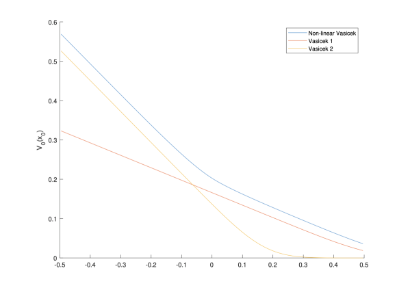
Figure 1. Numerically obtained prices for Asian put options. Blue is the non-linear Vasiček model (the upper line) and red and yellow are prices for Vasiček models without uncertainty, however parameters chosen in such a way that the mean reversion speed is either maximal or minimal, compare equations (37) and (38), respectively. On the $x$ axis we plot the initial value $x_{0}$.

Clearly, the initial value $x_{0}$ influences the value of the Asian put in such a way that a higher initial value implies on average a higher value of the integral $\int_{0}^{T}X(s)ds$, leading to lower prices for the put.

Let us first compare the two classical Vasiček models. The only difference is in the parameter $b^{1}$. However, for an intuition it is better to consider the mean reversion speed $\kappa=-b^{i}$ and the mean reversion level $\theta=\nicefrac{{b^{0}}}{{-b^{1}}}$. Note that by changing $b^{1}$ both models have different mean-reversion speed and mean-reversion level. In the model Vasiček 1, $\kappa=3$ and $\theta=0.05$, while in the model Vasiček 2, $\kappa=0.5$ and $\theta=0.3$. In the latter model, the mean-reversion level is at the upper boundary of the interval for $x_{0}$ (0.5) such that the process has the tendency to increase and the option shows a strong dependence from $x_{0}$ a little further away from $0.5$ (approx $0.2$ in our case). In Vasiček 1, the model mean-reverts strongly to $0.05$ and the dependence on the initial value is therefore less pronounced.

The price in the model under uncertainty (the non-linear Vasiček model) clearly dominates the prices without parameter uncertainty. Moreover, the value function shows a smoothed kink around $0$ which stems from the switching behaviour of the supremum in the non-linear Kolmogorov equation at $0$.

6. The numerical solution of functional PDEs

A full numerical study of the non-linear pricing of path-dependent options is far beyond the scope of this article. Our intention is to present a small numerical example which on the one side highlights the feasibility of the chosen numerical approach via deep neural networks and on the other side also shows the challenges of this approach.

While in the case of Asian options finite difference methods could be applied since the average has a smoothing effect, this will no longer be possible in other cases, for example when Barrier options are considered. For such options we propose to solve the equation numerically relying on machine learning methods. Essentially, the idea is to write the problem as a forward-backward SDE which we then discretize in time. The resulting functional derivatives are approximated with neural networks.

The proposed method bases on the recent work on E et al. (2017), Beck et al. (2019) and is surprisingly simple.

6.1. Barrier options

Barrier options are inherently path-dependent. We consider for simplicity digital barrier options, and choose the case of an up-and-in option. These products offer the payoff $1$ if the barrier $B$ is reached in the interval of consideration, $[0,T]$, and $0$ otherwise. In practice, such products are highly attractive because they often allow for cheaper investments (an up-and-in Call might be significantly cheaper in comparison to a standard Call). More precisely, the payoff is given by

$$\Phi(x_{T})={\mathds{1}}_{\{\sup_{s\in[0,T]}x(s)\geq B\}},\quad x\in C([0,T],{\mathcal{X}}),$$ (39)

In this case we are not able to reduce the value function to a classical PDE for $v$ since the non-anticipative functional

$$F_{t}(x_{t})=\sup_{s\in[0,t]}x(s)$$

is not vertically differentiable (consider $t>0$ and $x$ with ${\sup_{s\in[0,t]}x(s)=x(0)=x(t)}$).

We therefore propose an algorithm how to solve the (non-linear) functional Kolmogorov PDE in an approximate way by relying on machine learning techniques. Note that a Monte-Carlo simulation in this context is highly intractable because one has to simulate under all measures from $\mathcal{A}(t,x_{t},\Theta)$.

Moreover, solving the Kolmogorov equation (15) directly through numerical methods like finite differences face the challenge that pathwise derivatives have to be approximated by finite differences with requires a fine discretization of the path space $D([0,T])$. We begin by establishing the connection between functional PDEs and forward-backward stochastic differential equations (FBSDEs).

6.2. Backward SDEs

For an overview on backward stochastic differential equations we refer, for example, to Zhang (2017). Generally speaking, we are interested in functional PDEs of the form

$$\begin{split}{\mathcal{D}}_{t}F(x_{t})&=f\left(t,x(t),F(x_{t}),\nabla_{x}F_{t}(x_{t}),\nabla_{x}^{2}F_{t}(x_{t})\right)\quad\text{on }[0,T)\times C([0,T]),\\ F_{T}(x_{T})&=g(x_{T})\quad\forall x\in C([0,T])\end{split}$$ (40)

with a non-anticipative functional $F$, $T>0$ and mappings $f:[0,T]\times\mathbb{R}^{4}\to\mathbb{R}$ and $g:C([0,T])\to\mathbb{R}.$ Clearly, the non-linear Kolmogorov equation (15) falls into this class.

We consider a filtered probability space $(\Omega,{\mathscr{F}},\mathbb{F},P)$ together with a Brownian motion $W$. For the following we set $\nabla_{x}F_{T}=\nabla_{x}^{2}F_{T}:=0$.

Lemma 6.1.

Assume that the non-anticipate functional $F\in\mathbb{F}_{l}^{\infty}$ satisfies $F\in\mathbb{C}_{b}^{1,2}([0,T))$ and solves (40). With $x\in\mathbb{R}$ define the two processes

$$X(t) :=x+W(t)\quad\text{ and }\quad Y(t):=F_{t}(X_{t}),\qquad\quad t\in[0,T].$$

Then $Y$ solves the BSDE

$$Y(t)=g(X_{T}) -\int_{t}^{T}\left(f\left(s,X(s),Y(s),\nabla_{x}F_{s}(X_{s}),\nabla_{x}^{2}F_{s}(X_{s})\right)+\frac{1}{2}\nabla_{x}^{2}F_{s}(X_{s})\right)ds$$

$$-\int_{t}^{T}\nabla_{x}F_{s}(X_{s})dW(s)\quad P\text{-a.s. }\forall t\in[0,T].$$ (41)

Proof.

Observe that $F$ satisfies the assumptions of the functional Itô-formula, Theorem 4.1 in Cont and Fournié (2013). By this, we obtain that

$$Y(t) =Y(0)+\int_{0}^{t}\left({\mathcal{D}}_{s}F(X_{s})+\frac{1}{2}\nabla_{x}^{2}F_{s}(X_{s})\right)ds+\int_{0}^{t}\nabla_{x}F_{s}(X_{s})dW(s).$$

Since $F$ solves (40) by assumption, we obtain for all $t\in[0,T)$,

$$Y(t)=Y(0) +\int_{0}^{t}\left(f\left(s,X(s),Y(s),\nabla_{x}F_{s}(X_{s}),\nabla_{x}^{2}F_{s}(X_{s})\right)+\frac{1}{2}\nabla_{x}^{2}F_{s}(X_{s})\right)ds$$

$$+\int_{0}^{t}\nabla_{x}F_{s}(X_{s})dW(s)\quad P\text{-a.s.}$$

By continuity, this can be extended to $[0,T]$. Hence, for all $t\in[0,T]$,

$$Y(t) =Y(T)-(Y(T)-Y(t))=\eqref{eq:BSDE}.\qed$$

6.3. Deep learning of fractional gradients

Consider a discretization in time, $0=t_{0}<\dots<t_{N}=T$. The BSDE (41) is approixmated as follows

$$Y(t_{n+1}) \approx Y(t_{n})+\nabla_{x}F_{t_{n}}(X_{t_{n}})(W(t_{n+1})-W(t_{n}))$$

$$+\Big{(}f\left(t_{n},X(t_{n}),Y(t_{n}),\nabla_{x}F_{t_{n}}(X_{t_{n}}),\nabla_{x}^{2}F_{t_{n}}(X_{t_{n}})\right)+\frac{1}{2}\nabla_{x}^{2}F_{t_{n}}(X_{t_{n}})\Big{)}\,(t_{n+1}-t_{n})$$ (42)

with $Y(t_{N})=g(X_{t_{N}})$. We proceed as follows:

1. Choose random starting values $Y(t_{0})$, $\nabla_{x}F_{t_{0}}(X_{t_{0}})$ and $\nabla_{x}^{2}F_{t_{0}}(X_{t_{0}})$.

2. Approximate $\nabla_{x}F_{t_{n}}(X_{t_{n}})$ and $\nabla_{x}^{2}F_{t_{n}}(X_{t_{n}})$, $n=1,\dots,N-1$, via neural networks.

3. Repeat the following training step for the computation of a minibatch of size $M$ until a sufficient level of accuracy is reached:

   • Sample $M$ random paths $(X(t_{0}),\dots,X(t_{N}))$.

   • Use (1) to compute $m=1,\dots,M$ paths $(Y^{m}(t_{0}),\dots,Y^{m}(t_{N}))$.

   • Compute the aggregated loss $\sum_{m=1}^{M}(Y^{m}(t_{N})-g(X^{m}_{t_{N}}))^{2}$.

   • Update parameter of the neural net to minimize the loss function (for example by using stochastic gradient descent).

Algorithm 1 Outline of the Algorithm

As a next step we detail how neural networks can be used for deep-learning of the required gradients $\nabla_{x}F_{t}(X_{t})$ and $\nabla_{x}^{2}F_{t}(X_{t}).$ Consider a discrete time grid $0=t_{0}<\dots<t_{N}=T$. Since the solution $Y$ of (41) satisfies

$$E_{P}\big{[}(Y_{T}-g(X_{T}))^{2}\big{]}=0,$$

a discretized approximation $Y^{\theta}$ can be found by minimizing

$$\theta\mapsto E_{P}\big{[}(Y^{\theta}_{N}-g(X_{t_{0}},\dots,X_{t_{N}}))^{2}\big{]},$$

with the approximation $Y^{\theta}$ which we construct now. The associated loss function is $\ell(\theta)=(Y^{\theta}_{N}-g(X_{t_{0}},\dots,X_{t_{N}}))^{2}$. The value $g(X_{T})$ is approximated by the piecewise constant path of $X$ based on $X_{t_{0}},\dots,X_{t_{N}}$. We shortly denote this in the following by

$$g(X^{N}_{T}):=g(X_{t_{0}},\dots,X_{t_{N}}),$$

and similarly for other functions depending on the discretized approximation $X^{N}$ of $X$.

The parameter vector $\theta\in\mathbb{R}^{\nu},\nu\in\mathbb{N},$ contains initial values and the parameters of the neural networks and will be specified step by step.

Initial values

The first three values $(\theta_{1},\theta_{2},\theta_{3})$ denote the initial values where $\theta_{1}=Y_{0}^{\theta}$ approximates $Y_{t_{0}}$, $\theta_{2}$ approximates $\nabla_{x}F_{t_{0}}(X_{t_{0}})$ and $\theta_{3}$ approximates $\nabla_{x}^{2}F_{t_{0}}(X_{t_{0}}).$

Functional derivatives

Furthermore, we will use the neural networks $\mathscr{NN}^{1}_{n}=\mathscr{NN}^{1,\theta}_{n}$ as approximations of $\nabla_{x}F_{t_{n}}(X_{t_{n}})$, $n=1,\dots,N-1$; the neural networks $\mathscr{NN}^{2}_{n}=\mathscr{NN}^{2,\theta}_{n}$ approximate $\nabla_{x}^{2}F_{t_{n}}(X_{t_{n}})$.

More precisely, ${\mathscr{N}}_{n}^{1}:\mathbb{R}^{n}\to\mathbb{R}$ depends on the training parameters $\theta_{j_{n-1}+1},\dots,\theta_{i_{n}}$ while ${\mathscr{N}}_{n}^{2}:\mathbb{R}^{n}\to\mathbb{R}$ depends on the training parameters $\theta_{i_{n}+1},\dots,\theta_{j_{n}}$ with $j_{0}=3$.

Then, our approximation $Y^{N}$ is given by (compare equation (41)) $Y^{N}_{0}:=\theta_{1}$ and

$$Y_{n+1}^{N}:=Y_{n}^{N} +\left(f(t_{n},X(t_{n}),Y_{n}^{N},\mathscr{NN}_{n}^{1}(X^{N}_{t_{n}}),\mathscr{NN}_{n}^{2}(X^{N}_{t_{n}}))+\frac{1}{2}\mathscr{NN}_{n}^{2}(X^{N}_{t_{n}})\,\right)(t_{n+1}-t_{n})$$

$$+\mathscr{NN}_{n}^{1}(X^{N}_{t_{n}})\cdot(W(t_{n+1})-W(t_{n})),$$

$n=1,\dots,N-1$.

Optimization

As mentioned above the goal of the algorithm is to find $\theta$ such that the expected loss is minimized. To achieve this a batch of size $M$ of simulations is constructed and for each simulation $m$, the loss is given by

$$\ell_{m}(\theta):=(Y^{m,\theta}_{N}-g(X^{m}_{t_{0}},\dots,X^{m}_{t_{N}}))^{2}.$$

The expectation is estimated by the aggregated loss

$$\ell(\theta)=\sum_{m=1}^{M}\ell_{m}(\theta).$$

Now the parameter $\theta$ can be minimized as detailed in Algorithm 1 by, for example, stochastic gradient descent. The targeted approximation of $Y(0)=F_{0}(X_{0})$ is the parameter $\theta_{1}$.

6.4. Numerical results

Our experiments showed that if the network is chosen too deep, the parameter $\theta_{1}$ (which is the one which we are mainly interested in) will be less efficiently trained or even not trained at all. For our goals, neural networks with 4 layers and rectified linear units (ReLU) as activation function achieved the best results.

For the numerical results of pricing up-and-in digital options (compare equation (39)) we consider the case already studied in the previous section, where we chose the parameters according to equation (37).

$x(0)$		-0.3	-0.2	-0.1	0	0.1	0.2	0.3
mean		0.607	0.665	0.732	0.790	0.856	1.000	1.000
std.dev.		0.008	0.006	0.005	0.004	0.002	0.003	0.003

Table 1. Computed prices of the barrier up-and-in digital options (10 runs) with associated standard deviations for different initial values $x(0)$ of the non-linear affine process $X$. The model parameters are specified in equation (37). In most cases the optimal value is already achieved after 25.000 steps, the values here are computed with 100.000 steps, however.

The outcome of the numerical deep learning algorithm is shown in Table 1. The algorithm computes, as described above the value $V_{0}(x_{0})$ of the digital up-and-in barrier option as detailed in (39). Since the outcome of the algorithm is random, we simulated it 10 times and show mean together with standard deviation. Clearly, as expected, prices are increasing in $x_{0}$. For high initial value we face small difficulties as for $x(0)=0.2$ the value should of course be exactly equal to $1$. For even higher values, the price remains similar.

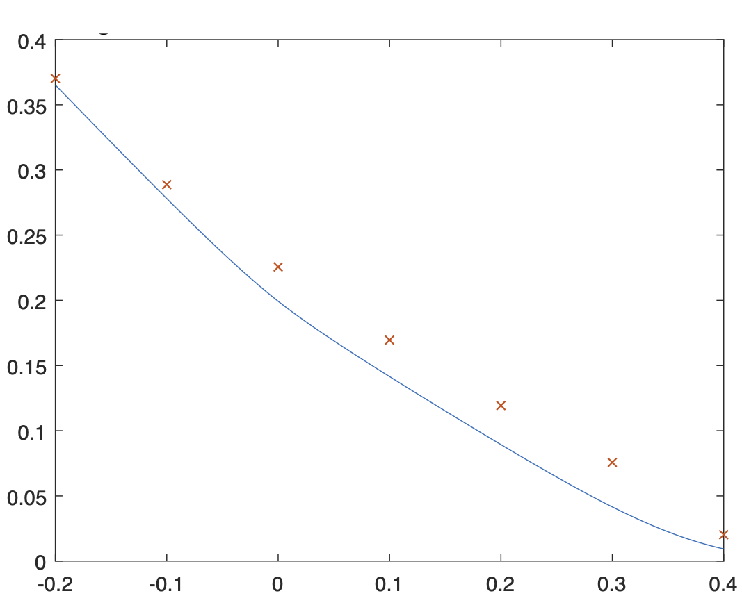
Figure 2. Comparison of the finite difference method (solid line, blue) with the deep-learning approach (crosses) in the context of Asian put options according to the model detailed in equation (43).

Benchmarking

To obtain a comparison with existing methods we revisit the Asian put and compare the results from the machine-learning algorithm with the results from finite difference schemes, which are shown in Figure 2. The chosen parameters are:

$$\text{\text@underline{$\gamma$}}=\bar{\gamma}=\frac{1}{2},\ \text{\text@underline{$b$}}^{0}=0.05,\ \bar{b}^{0}=0.15,\ \text{\text@underline{$b$}}^{1} =-3,\ \bar{b}^{1}=-0.5,\ \text{\text@underline{$a$}}^{0}=0.01,\ \bar{a}^{0}=0.02,\ \text{\text@underline{$a$}}^{1}=\bar{a}^{1}=0,$$ (43)

with $T=0.5$ and $K_{1}=0.2,\ K_{2}=10^{6}$.

We can make the following observations:

1. The machine-learning algorithm produces slightly higher values in comparison to the finite difference scheme. The typical kink at $x(0)=0$ is very well visible. The difference is more pronounced in the middle of the observation area, i.e. between $0.1$ and $0.3$.

2. Clearly, the approximation of $g(X_{T})$ with a finite number of gridpoints and piecewise constant extrapolation will cause difficulties when this approximation fails to reach $g(X_{T})$. In the cases we consider here, this does not cause problems.

References

- (1)
- Acciaio et al. (2016) Acciaio, B., Beiglböck, M., Penkner, F. and Schachermayer, W. (2016), ‘A model-free version of the fundamental theorem of asset pricing and the super-replication theorem’, Mathematical Finance 26(2), 233–251.
- Bayraktar and Xing (2011) Bayraktar, E. and Xing, H. (2011), ‘Pricing Asian options for jump diffusion’, Mathematical Finance 21(1), 117–143.
- Beck et al. (2019) Beck, C., E, W. and Jentzen, A. (2019), ‘Machine learning approximation algorithms for high-dimensional fully nonlinear partial differential equations and second-order backward stochastic differential equations’, Journal of Nonlinear Science 29(4), 1563–1619.
- Bergenthum and Rüschendorf (2007) Bergenthum, J. and Rüschendorf, L. (2007), ‘Comparison of semimartingales and Lèvy processes’, The Annals of Probability 35(1), 228–254.
- Bertsekas and Shreve (1978) Bertsekas, D. P. and Shreve, S. E. (1978), Stochastic Optimal Control: The Discrete Time Case, Acadamic Press.
- Biagini and Oberpriller (2021) Biagini, F. and Oberpriller, K. (2021), ‘Reduced-form setting under model uncertainty with non-linear affine intensities’, Probability, Uncertainty and Quantitative Risk 6(3), 159–188.
- Bielecki et al. (2018) Bielecki, T. R., Cialenco, I. and Rutkowski, M. (2018), ‘Arbitrage-free pricing of derivatives in nonlinear market models’, Probability, Uncertainty and Quantitative Risk 3(1), 2.
- Cont (2006) Cont, R. (2006), ‘Model uncertainty and its impact on the pricing of derivative instruments’, Mathematical Finance 16, 519–542.
- Cont and Fournié (2013) Cont, R. and Fournié, D.-A. (2013), ‘Functional Itô calculus and stochastic integral representation of martingales’, The Annals of Probability 41(1), 109–133.
- Criens and Niemann (2022a) Criens, D. and Niemann, L. (2022a), ‘Markov selections and Feller properties of nonlinear diffusions’, arXiv preprint arXiv:22051.15200v1 .
- Criens and Niemann (2022b) Criens, D. and Niemann, L. (2022b), ‘Non-linear continuous semimartingales’, arXiv preprint arXiv:2204.07823 .
- Denis and Martini (2006) Denis, L. and Martini, C. (2006), ‘A theoretical framework for the pricing of contingent claims in the presence of model uncertainty’, The Annals of Applied Probability 16(2), 827–852.
- Denk et al. (2020) Denk, R., Kupper, M. and Nendel, M. (2020), ‘A semigroup approach to nonlinear Lévy processes’, Stochastic Processes and their Applications 130(3), 1616–1642.
- Duffie et al. (2003) Duffie, D., Filipović, D. and Schachermayer, W. (2003), ‘Affine processes and applications in finance’, Ann. Appl. Probab. 13, 984–1053.
- E et al. (2017) E, W., Han, J. and Jentzen, A. (2017), ‘Deep learning-based numerical methods for high-dimensional parabolic partial differential equations and backward stochastic differential equations’, Communications in Mathematics and Statistics 5(4), 349–380.
- El Karoui and Tan (2015) El Karoui, N. and Tan, X. (2015), ‘Capacities, measurable selection and dynamic programming part II: Application in stochastic control problems’, arXiv:1310.3364v2 .
- Fadina et al. (2019) Fadina, T., Neufeld, A. and Schmidt, T. (2019), ‘Affine processes under parameter uncertainty’, Probability, Uncertainty and Quantitative Risk 4(1), 1.
- Guyon and Henry-Labordère (2013) Guyon, J. and Henry-Labordère, P. (2013), Nonlinear option pricing, CRC Press.
- Janson and Tysk (2006) Janson, S. and Tysk, J. (2006), ‘Feynman-Kac formulas for Black-Scholes-type operators’, Bulletin of the London Mathematical Society 38(2), 269–282.
- Jeanblanc et al. (2009) Jeanblanc, M., Yor, M. and Chesney, M. (2009), Mathematical methods for financial markets, Springer Finance, Springer-Verlag London Ltd., London.
- Kallenberg (2002) Kallenberg, O. (2002), Foundations of modern probability, Probability and its Applications (New York), second edn, Springer-Verlag, New York.
- Karatzas and Shreve (1988) Karatzas, I. and Shreve, S. E. (1988), Brownian Motion and Stochastic Calculus, Springer Verlag. Berlin Heidelberg New York.
- Keller-Ressel et al. (2019) Keller-Ressel, M., Schmidt, T., Wardenga, R. et al. (2019), ‘Affine processes beyond stochastic continuity’, The Annals of Applied Probability 29(6), 3387–3437.
- Kirkby and Nguyen (2020) Kirkby, J. L. and Nguyen, D. (2020), ‘Efficient Asian option pricing under regime switching jump diffusions and stochastic volatility models’, Annals of Finance 16(3), 307–351.
- Lütkebohmert et al. (2022) Lütkebohmert, E., Schmidt, T. and Sester, J. (2022), ‘Robust deep hedging’, Quantitative Finance 22(8), 1465–1480.
- Muhle-Karbe and Nutz (2018) Muhle-Karbe, J. and Nutz, M. (2018), ‘A risk-neutral equilibrium leading to uncertain volatility pricing’, Finance and Stochastics 22(2), 281–295.
- Neufeld and Nutz (2014) Neufeld, A. and Nutz, M. (2014), ‘Measurability of semimartingale characteristics with respect to the probability law’, Stochastic Processes and their Applications 124(11), 3819 – 3845.
- Neufeld and Nutz (2017) Neufeld, A. and Nutz, M. (2017), ‘Nonlinear Lévy processes and their characteristics’, Transactions of the American Mathematical Society 369(1), 69–95.
- Peng (2019) Peng, S. (2019), Nonlinear expectations and stochastic calculus under uncertainty: with robust CLT and G-Brownian motion, Vol. 95, Springer Nature.
- Zhang (2017) Zhang, J. (2017), Backward stochastic differential equations, Springer.