Probing Physics Beyond the Standard Model: Limits from BBN and the CMB Independently and Combined

Abstract

We present new Big Bang Nucleosynthesis (BBN) limits on the cosmic expansion rate or relativistic energy density, quantified via the number $N_{\nu}$ of equivalent neutrino species. We use the latest light element observations, neutron mean lifetime, and update our evaluation for the nuclear rates $d+d\rightarrow\mbox{${}^{3}{\rm He}$}+n$ and $d+d\rightarrow\mbox{${}^{3}{\rm H}$}+p$. Combining this result with the independent constraints from the cosmic microwave background (CMB) yields tight limits on new physics that perturbs $N_{\nu}$ and $\eta$ prior to cosmic nucleosynthesis: a joint BBN+CMB analysis gives $N_{\nu}=2.898\pm 0.141$, resulting in $N_{\nu}<3.180$ at $2\sigma$. We apply these limits to a wide variety of new physics scenarios including right-handed neutrinos, dark radiation, and a stochastic gravitational wave background. The strength of the independent BBN and CMB constraints now opens a new window: we can search for limits on potential changes in $N_{\nu}$ and/or the baryon-to-photon ratio $\eta$ between the two epochs. The present data place strong constraints on the allowed changes in $N_{\nu}$ between BBN and CMB decoupling; for example, we find $-0.708<N_{\nu}^{\rm CMB}-N_{\nu}^{\rm BBN}<0.328$ in the case where $\eta$ and the primordial helium mass fraction $Y_{p}$ are unchanged between the two epochs; we also give limits on the allowed variations in $\eta$ or in $(\eta,N_{\nu})$ jointly. We discuss scenarios in which such changes could occur, and show that BBN+CMB results combine to place important constraints on some early dark energy models to explain the $H_{0}$ tension. Looking to the future, we forecast the tightened precision for $N_{\nu}$ arising from both CMB Stage 4 measurements as well as improvements in astronomical ${}^{4}{\rm He}$ measurements. We find that CMB-S4 combined with present BBN and light element observation precision can give $\sigma(N_{\nu})\simeq 0.03$. Such future precision would reveal the expected effect of neutrino heating ($N_{\rm eff}-3=0.044$) of the CMB during BBN, and would be near the level to reveal any particle species ever in thermal equilibrium with the standard model. Improved $Y_{p}$ measurements can push this precision even further.

1 Introduction

Big-bang nucleosynthesis (BBN) is the theory which accounts for the production of the lightest nuclei [1] during the first seconds to minutes of cosmic time (for reviews see refs. [2, 3, 4, 5, 6, 7]). The physics behind standard BBN is very well known because the typical energy scale is that of relatively low-energy nuclear physics, i.e., of order 1 MeV. We refer to standard BBN (SBBN) as the theory based on the Standard Model of particle and nuclear interactions, and $\Lambda$CDM cosmology with three neutrino flavors. At present, SBBN is the earliest reliable probe the universe where the microphysics is well understood. All four fundamental interactions participate in element formation, so SBBN probes all known interactions. Moreover, through the effects of the cosmic expansion rate, BBN is sensitive to all contributions to cosmic mass-energy density [9, 10, 11, 12] which can often be parameterized as additional neutrino flavors and as we will see allows one to probe departures from the Standard Model.

In the pioneering work of Steigman, Schramm, and Gunn [12], the existence of additional massive charged leptons was assumed to be accompanied by (massless) neutrinos. As such, these would contribute to the radiation energy density prior to nucleosynthesis,

$$\rho_{R}=\rho_{\gamma}+\rho_{e}+\rho_{\nu}=\frac{\pi^{2}}{30}\left(2+\frac{7}{2}+\frac{7}{4}N_{\nu}\right)T^{4}\,,$$ (1.1)

for temperatures $T\gtrsim 1$ MeV, where $N_{\nu}$ is the total number of neutrino flavors (relativistic at temperature $T$). More generally, the presence of any additional relativistic particle species can be expressed in terms of the equivalent number $N_{\nu}$.

The best accelerator limit on the number of neutrino species is based on the invisible width of the $Z^{0}$ boson. The LEP experiments combined give $N_{\nu}=2.9963\pm 0.0074$ [13]; this of course is in impressive agreement with the $N_{\nu}^{\rm SM}=3$ result from the Standard Model. Note that this limit applies to particles that have standard electroweak couplings to the $Z^{0}$, whereas the BBN (and CMB) limits probe any species in thermal equilibrium during this epoch. The cosmological limits are thus complementary to the accelerator results in that they are arise from different physics, and importantly, these probes can give different results. We will refer to BBN with $N_{\nu}\neq 3$ as “NBBN”.

As is well known, the abundances of the light elements produced in BBN are very sensitive to the neutron-proton ratio $(n/p)$, when the deuterium bottleneck is broken at $T\sim 0.1$ MeV. While the helium abundance is very sensitive to this ratio (as nearly all free neutrons end up in a ${}^{4}{\rm He}$ nucleus), the deuterium abundance is also sensitive to $(n/p)$. The neutron-to-proton ratio is largely determined at the freeze-out of the weak interaction rates (modulo neutron decays). The freeze-out temperature in turn can be determined roughly by balancing the weak interaction rates with the expansion rate of the Universe, $\Gamma_{\rm weak}(T_{f})=H(T_{f})$, where $H$ is the Hubble parameter. Furthermore, we can approximate

$$\Gamma_{\rm weak}(T) \propto G_{F}^{2}T^{5}$$ (1.2)

$$H^{2}(T) \simeq \frac{8\pi}{3}G_{N}\rho_{R}\,,$$ (1.3)

where $G_{F,N}$ represent Fermi’s and Newton’s constants. Clearly, any change in the number of relativistic degrees of freedom, will affect $H$ and through $T_{f}$ will alter $(n/p)_{f}\sim e^{-\Delta m/T_{f}}$, where $\Delta m=1.29$ MeV is the neutron-proton mass difference. It is not hard to convince oneself that an increase in $N_{\nu}$ will lead to a larger value for $(n/p)_{f}$ and hence a larger value for the the ${}^{4}{\rm He}$ mass fraction, denoted as $Y_{p}$. More generally, any departure from the Standard Model (of either particle/nuclear physics or cosmology) which affects either $\Gamma_{\rm weak}$ or $H$, will alter the light element abundances.

Of course, constraints on new physics requires accurate abundance measurements, accurate nuclear rates, as well as an accurate determination of the baryon density, $\Omega_{b}h^{2}$, or baryon-to-photon ratio, $\eta$. The baryon density has indeed been determined very accurately first by WMAP [14] and subsequently by Planck [8], effectively making SBBN a parameter-free theory [15]. The deuterium abundance, observed in high redshift quasar absorption systems, is now determined with approximately 1% accuracy, [16, 17, 18, 19, 20, 21, 22, 23] giving

$$\left(\frac{\rm D}{\rm H}\right)_{\rm obs}=(2.55\pm 0.03)\times 10^{-5}\,.$$ (1.4)

Because of the small uncertainty in its observational determination, deuterium, which scales as $N_{\nu}^{0.405}$ [24, 25], now plays an important role in containing physics beyond the Standard Model. Historically however, it is ${}^{4}{\rm He}$ which has set the strongest constraints on $N_{\nu}$. ${}^{4}{\rm He}$ is observed in extragalactic HII regions using a series of ${}^{4}{\rm He}$ and H emission lines. The observational determination of ${}^{4}{\rm He}$ has also improved [26, 27]. A recent analysis including high quality observations of the Leoncino dwarf galaxy leads to an inferred primordial abundance of [28]

$$Y_{p,\rm obs}=0.2448\pm 0.0033\,.$$ (1.5)

Similar recent analyses yield $0.2453\pm 0.0034$ [27], $0.2436\pm 0.0040$ [29], and $0.2462\pm 0.0022$ [30]. The helium abundance scales as $Y_{p}\propto N_{\nu}^{0.163}$ [24]. For comparison, using the Planck likelihood chains [8] with fixed $N_{\nu}$, SBBN leads to mean values [25] of

$$\left(\frac{\rm D}{\rm H}\right)_{\rm SBBN} = (2.506\pm 0.110)\times 10^{-5}$$ (1.6)

$$Y_{p,\rm SBBN} = 0.2469\pm 0.0002\,.$$ (1.7)

CMB anisotropies, particularly at high multipoles, are sensitive to the neutrino number via the effects on the expansion rate, and via the ratio of the photon diffusion length to the sound horizon (see, e.g., ref. [31]). In the Standard Model, the effective number of neutrino species $N_{\rm eff}$ is 3.044 [32, 33, 34, 35]. The difference

$$\Delta N_{\nu,\ \nu-\rm heating}=N_{\rm eff}-3=0.044$$ (1.8)

is due to residual heating to neutrinos when accounting for the fact the $e^{+}e^{-}$ annihilation in the early universe is not instantaneous, and has a branching to $e^{+}e^{-}\rightarrow\nu\bar{\nu}$. In our notation, $N_{\rm eff}^{\rm SM}=3.044$ is equivalent to $N_{\nu}^{\rm SM}=3$ in the standard case. Eq. (1.8) thus sets an important target for measurements of $\Delta N_{\nu}$.

Another target for $N_{\nu}$ measurements comes from the presence of particles beyond the Standard Model; here too there is an important physically motivated limit (see, e.g., the recent review and forecasts in ref. [36]). A new species $X$, in equilibrium, has energy density

$$\rho_{X}=g_{X,\rm eff}\frac{\pi^{2}}{30}\ T_{X}^{4}$$ (1.9)

where $g_{X,\rm eff}$ is the number of degrees of freedom for scalars and 7/8 times the number of degrees of freedom when $X$ is a fermion. At high temperatures, if $X$ is in equilibrium with the SM thermal bath, $T_{X}=T_{\gamma}$. However if $X$ drops out of equilibrium, entropy conservation gives $T_{X}$ at lower temperatures

$$\frac{T_{X}}{T_{\gamma}}=\left(\frac{g_{*}(T_{\nu,\rm f})}{g_{*}(T_{X,\rm f})}\right)^{1/3}\times\left(\frac{4}{11}\right)^{1/3}\,,$$ (1.10)

where $g_{*}(T_{\nu,\rm f})=43/4$ is the number of SM degrees of freedom when neutrinos freeze out and $g_{*}(T_{X,\rm f})$ counts the number of effective degrees of freedom (not including $X$) when $X$ freezes out. We can relate the density in $X$ to an effective contribution to $N_{\nu}$ by defining

$$\Delta N_{\nu}=\frac{4}{7}g_{X,\rm eff}\left(\frac{T_{X}}{T_{\nu}}\right)^{4}$$ (1.11)

recalling that $(T_{\nu}/T_{\gamma})^{3}=4/11$. Thus the earlier a new species $X$ freezes out from the Standard Model, the lower its contribution to $\Delta N_{\nu}$ due to the resulting dilution of $g_{*}$:

$$\Delta N_{\nu} = \frac{4}{7}g_{X,\rm eff}\left[\frac{43}{4g_{*}(T_{X,\rm f})}\right]^{4/3}$$ (1.12)

$$\geq 0.027\ g_{X,\rm eff}$$ (1.13)

where the limiting value in Eq. (1.13) assumes that the species freezes out before the entire Standard Model, i.e., $g_{*}(T_{X,\rm f})=427/4$; later freeze-out will give higher $\Delta N_{\nu}$. We see that this limit is comparable to the neutrino heating perturbation in Eq. (1.8).

Including particles beyond the Standard Model increases the maximum possible $g_{*}$. In the extreme case, where new fields decouple so early that there entropy is diluted by the field content of a (supersymmetric) grand unified theory, many new (nearly) massless fields are allowed. For example, in minimal supersymmetric SU(5), $g_{*}(T_{X,\rm f})=1545/4$, the one-sided limit of $\delta N_{\nu}<0.226$ (see below) would place a limit of roughly 47 new scalars or 54 fermionic degrees of freedom. This may constrain some string theories which predict large numbers of light moduli [37].

In recent years, the cosmic microwave background (CMB) measurements have also become a probe of $N_{\nu}$ at the epoch of recombination. Allowing $N_{\nu}$ to vary, the Planck likelihood chains [8] lead to a determination of $\Omega_{\rm b}^{\rm CMB}h^{2}=0.02224\pm 0.00022$ corresponding to $\eta^{\rm CMB}=(6.090\pm 0.061)\times 10^{-10}$, and an effective number of neutrino flavors

$$N_{\nu}^{\rm CMB}=2.800\pm 0.294\,.$$ (1.14)

When $N_{\nu}$ is allowed to vary ($N_{\nu}\neq 3$), the NBBN calculations of D/H and $Y_{p}$ are somewhat different [25]

$$\left(\frac{\rm D}{\rm H}\right)_{\rm NBBN} = (2.447\pm 0.137)\times 10^{-5}$$ (1.15)

$$Y_{p,\rm NBBN} = 0.2441\pm 0.0041\,.$$ (1.16)

Note that both are still in very good agreement with observations. Also note that the theory uncertainty in $Y_{p}$ is now significantly larger due to the strong dependence of $Y_{p}$ on $N_{\nu}$. The combined result for NBBN convolved with the CMB chains gives [25] $\eta^{\rm NBBN+CMB}=6.092\pm 0.054$ and

$$\left.N_{\nu}\right|_{\rm Yeh2021}^{\rm BBN+CMB}=2.880\pm 0.144\,.$$ (1.17)

This result is updated in §4 below.

In this work, we make use of the analyses described in detail in [38, 39, 40, 6, 24]. Recently, there has been a burst of activity in response to new precision measurement of the $d(p,\gamma)\mbox{${}^{3}{\rm He}$}$ reaction by the LUNA collaboration [41]. Recent BBN studies have used two different approaches to nuclear rates: an empirical approach, based primarily on experimentally measured cross sections, finds excellent BBN+CMB agreement [42, 25], while an approach incorporating nuclear theory finds some tension [43]. Additional deuterium reaction measurements are called for to resolve this discrepancy [44]. Our work here is an extension of that in ref. [25] and we note that when the measured nuclear rates are used there is good agreement with the CMB. On the other hand, there is a primordial lithium problem–that is, the predicted BBN ${}^{7}{\rm Li}$/H differs significantly from observations [45, 46]. However, much of the evidence in support of associating the ${}^{7}{\rm Li}$ observed in low metallicity halo stars with primordial Li, has evaporated [47]. Recent non-observations of ${}^{6}{\rm Li}$ in halo stars provide new evidence that stellar depletion is at play, and thus offer new support for a stellar solution to the problem [47]. As such, in this paper we assume that the Li problem solution lies not in new physics, but elsewhere, most likely astrophysical–stellar depletion see e.g. [48, 49, 50, 51, 52, 53, 54, 55].

We calculate our results using a series of interlocking codes, beginning with the BBN calculation of light-element abundances, which form the basis for Monte Carlo runs that inform the likelihood functions described below. Our BBN code descends from the original Wagoner code [56], with updates for higher-order corrections to the weak rates [57] and for integration accuracy [58], as described more fully in ref. [59]. The Monte Carlo calculation and likeihood analysis stems from refs. [15, 40], and nuclear reaction rates have been continually updated, most recently in ref. [25] as well as $d+d$ rates as discussed below. A comparison with work by other groups shows that when the same nuclear rates are adopted, all light-element predictions in are in excellent agreement [60].

In this paper we build on the analysis of [24, 25]. We use updated nuclear rates for $d(d,n)$${}^{3}{\rm He}$ and $d(d,p)t$, as well as the updated ${}^{4}{\rm He}$ abundance [27] and neutron mean-life [61]. As in [62, 63, 64, 65], we concentrate on NBBN to first set constraints on $N_{\nu}$ and apply these constraints to a wide variety of extensions of the Standard Model. We focus on models where these extensions can be described as perturbations away from the SBBN with $N_{\nu}^{\rm SM}=3$ neutrino species. In some scenarios there can be changes to the microphysics of element formation due to new particles or interactions and these require a dedicated analysis beyond the scope of this paper.

In what follows, we perform a combined CMB+NBBN likelihood analysis in order to constrain $N_{\nu}$ and a host of extensions beyond the Standard Model. As we will see, D/H is now important in determining $N_{\nu}$, and as such, we first update nuclear rates for deuterium in §2. We then provide in §3 a brief summary of our likelihood analysis providing first limits from NBBN separately from those derived from the CMB. Next in §4, we provide our combined (CMB-NBBN) likelihood analysis and consider traditional limits on $N_{\nu}$ where no new physics is assumed between the epoch of BBN and CMB decoupling. We also allow different values of $N_{\nu}$ between BBN and CMB decoupling in §5. In §6 we anticipate the ability of future CMB-S4 and astronomical ${}^{4}{\rm He}$ measurements to further sharpen our measures of $N_{\nu}$, possibly even revealing the predicted standard neutrino heating effects. Our summary and conclusions are given in §7.

2 Re-evaluation of $d(d,n)\mbox{${}^{3}{\rm He}$}$ and $d(d,p)t$ Thermonuclear Rates

It has long been known that $d(p,\gamma)\mbox{${}^{3}{\rm He}$}$, $d(d,n)\mbox{${}^{3}{\rm He}$}$, and $d(d,p)t$ dominate the error of the BBN deuterium prediction [6]. Until recently, $d(p,\gamma)\mbox{${}^{3}{\rm He}$}$ was the major source of the D/H uncertainty due to its sparse cross section data with relatively large errors at BBN energies [25]. However, the precision cross section measurement from the LUNA Collaboration [41] revolutionized the evaluation of the $d(p,\gamma)\mbox{${}^{3}{\rm He}$}$ thermonuclear rate and its uncertainty. Including the LUNA data in our world average, we reported a new $d(p,\gamma)\mbox{${}^{3}{\rm He}$}$ rate with a factor of 2 improvement in its uncertainty, and went on to sow the impact of this new rate on the BBN prediction for D/H as well as constraints on relevant cosmological parameters [25]. Similar studies were performed in [42, 43].

Given the importance of precision D/H calculations for $\eta$ and (to a lesser extent) for $N_{\nu}$ determinations, we want to evaluate all of the important deuterium destruction rates on the same footing. Prior to the new LUNA data, we had adopted deuterium rates based on NACRE-II [66]. Having the updated $d(p,\gamma)\mbox{${}^{3}{\rm He}$}$ rate that incorporates the new LUNA data, we will now go one step further; we apply the same methodology and global fitting procedure of ref. [25] to re-evaluate $d(d,n)\mbox{${}^{3}{\rm He}$}$ and $d(d,p)t$ rates and uncertainties in this study. In this section we summarize the results of this analysis.

Fortuitously, $d(d,n)\mbox{${}^{3}{\rm He}$}$ and $d(d,p)t$ share the same initial state, and so can be measured in the same experiment. Because we aim to re-evaluate these two $d+d$ rates with our new procedure, we use the similar datasets adopted in NACRE-II [66]. We include cross section data for $d(d,n)\mbox{${}^{3}{\rm He}$}$ and $d(d,p)t$ from Schulte et al. [67], Krauss et al. [68], Brown et al. [69], Greife et al. [70], Leonard et al. [71], and Tumino et al. [72]. In addition, we add data from Ganeev et al. [73] and Hofstee et al. [74], who only report results for $d(d,n)\mbox{${}^{3}{\rm He}$}$. To avoid the impact of the laboratory electron screening effect at low energies, we adopt data points above 10 keV, which is also below the Gamow window for $d+d$. For the high energy end, we stop at 3 MeV because it sufficiently covers the most important energy ranges for both BBN $d+d$ rates. These adopted data are plotted in Figures 1 and 2 in terms of the astrophysical $S$-factor $S(E)=E\sigma(E)e^{2\pi\eta_{s}}$ versus the center-of-mass energy $E$ to factor out the effect of the Coulomb barrier, where $\eta_{s}=e^{2}/\hbar v$ is the Sommerfeld parameter and $v=v(E)$ is the relative velocity of reactant D nuclides, and $\sigma(E)$ is the reaction cross section. In Figure 2, we show the $S$-factor for the $d+d$ reactions as in Fig. 1, but for wider and logarithmic energy scale. We see that our fits agrees with the experimental data out to $\sim 2\ \rm MeV$. Larger energies are sufficiently beyond the range of validity of our 4th-order polynomial description that the fit becomes unphysical.

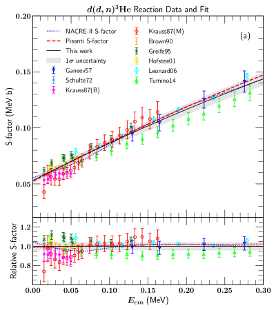
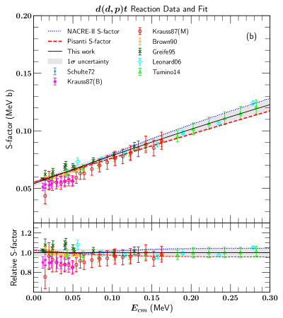
Figure 1: The astrophysical $S$-factor for $d(d,n)$${}^{3}{\rm He}$ in the left panel and $d(d,p)t$ in the right panel. On a linear energy scale centered at the BBN energies, we show for both $d+d$ rates 1) the NACRE-II [66] $S$-factor used in our previous BBN analysis [24] (blue dotted); 2) the global average from Pisanti et al. [42] (red dashed); and 3) our new world average rate (black solid).

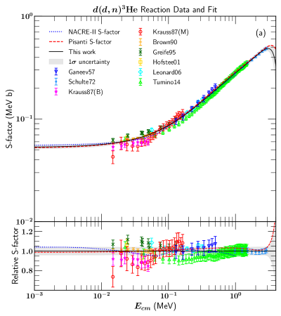
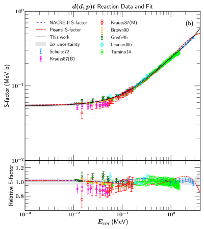
Figure 2: The astrophysical $S$-factor for $d(d,n)$${}^{3}{\rm He}$ in the left panel and $d(d,p)t$ in the right panel on a log energy scale centered at the BBN energies.

Following the same nuclear cross section fitting procedure developed for $d(p,\gamma)\mbox{${}^{3}{\rm He}$}$ [25], we fit the $S$-factor using a series of polynomials in terms of center-of-mass energy $E$. Because both $d(d,n)\mbox{${}^{3}{\rm He}$}$ and $d(d,p)t$ $S$-factor plots show smooth behavior around BBN energy range, we found that a polynomial expansion including a 4th-order ($E^{4}$) term agrees well with the data without overfitting for both reactions. The global best fit is determined by $\chi^{2}$ minimization. Beyond the experimental energy-dependent uncertainty (statistical and systematic errors combined in quadrature), we also include an energy-independent uncertainty to account for the systematic discrepancies among datasets [38]. The resulting $\chi^{2}$ per degree of freedom is around unity with the inclusion of such a discrepancy error.

We also present in Figures 1 and 2 relevant $S$-factor fits for both $d(d,n)\mbox{${}^{3}{\rm He}$}$ (on the left panel) and $d(d,p)t$ (on the right panel) considered in this paper as a function of energy. The blue dotted curve is from NACRE-II [66] and was adopted in our previous BBN studies [6, 24, 25]. The black solid curve is our new average rate with the grey shaded region for our calculated 1-$\sigma$ uncertainty. For comparison, the work done here is basically re-evaluating the $d+d$ rates based on a dataset selection similar to NACRE-II but using our own fitting procedure. Figure 1 shows that the NACRE-II and our new cross section fits agree with each other and the data within uncertainties at BBN energies. Moreover, Pisanti et al. have recently reported their latest fits for both $d+d$ rates based on a similar empirical polynomial fitting procedure [42]. We include their fit in Figures 1 and 2 using the red dashed curve for data analysis method comparison. In the lower portion of these two panels, the data and other fits are shown relative to new fit used here.

Once we have the best fit for the $S$-factor, we can calculate the average thermonuclear rate as a function of temperature $T$ using

$$\lambda(T)=N_{\rm Avo}\langle\sigma v\rangle=N_{\rm Avo}\bigg{(}\frac{8}{\mu\pi}\bigg{)}^{1/2}(kT)^{-3/2}\int^{E_{\rm max}}_{E_{\rm min}}S(E)e^{-2\pi\eta_{s}}e^{-E/kT}dE,$$ (2.1)

where $N_{\rm Avo}$ is Avogadro’s number and $\mu$ is the reduced mass. The integration bounds are set to be ($E_{\rm min}$, $E_{\rm max}$) = (0 $kT$, 100 $kT$) for practical calculation.

In Figure 3, using our new rates as baselines, we show the relative $d+d$ thermal rates for our previous work [6, 24, 25] calculated from the fits of NACRE-II. Our new rates are consistent with NACRE-II rates around $T_{9}=1$, which is at the heart of BBN deuterium synthesis. In fact, within uncertainty, the $d(d,n)\mbox{${}^{3}{\rm He}$}$ rate from NACRE-II is a few percent smaller than our new baseline at $0.1<T_{9}<1$, but for $d(d,p)t$ the trend goes in the opposite direction. Because these two $d+d$ rates have similar scaling relations to the deuterium prediction [25], the downward and upward differences shown in the panels of Figure 3 at $0.1<T_{9}<1$ almost cancel in practice. Thus we do not expect large changes in the mean values of D/H calculated with our updated network versus the our older work. But in our new analysis, the predicted deuterium uncertainty contributions have decreased by a factor of $\sim 1.5$ from $d(d,n)\mbox{${}^{3}{\rm He}$}$ and a factor of $\sim 1.4$ from $d(d,p)t$. Therefore, we anticipate that the the resulting full D/H uncertainty will be lower by a similar factor.

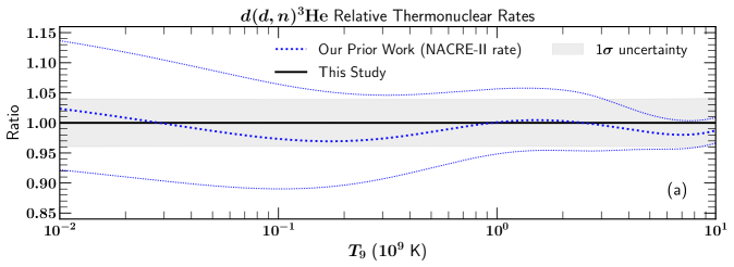
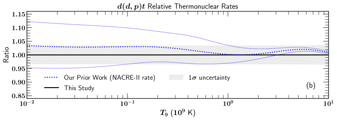
Figure 3: The comparison between the old thermonuclear rates adopted in our prior work [6, 24, 25] and our new averages as baselines for $d(d,n)$${}^{3}{\rm He}$ in the left panel and $d(d,p)t$ in the right panel. The old rates, calculated from NACRE-II [66], are in dotted blue with 1$\sigma$ bounds. The 1$\sigma$ uncertainties of new rates are indicated by the grey regions. Curves are shown as a function of temperature in units of $T_{9}=10^{9}$ K. Our new rates are consistent with the old rates around $T_{9}=1$.

2.1 Primordial Light Element Abundance Predictions

Using the baryon density from the base_yhe_plikHM_TTTEEE_lowl_lowE_post_lensing chains of Planck 2018 data as input for the $N_{\nu}=3$ standard case, here we list our latest SBBN light element abundance predictions with their means and $1\sigma$ errors:

$$Y_{p} = 0.2467\pm 0.0002,$$ (2.2)

$${\rm D/H} = (2.506\pm 0.083)\times 10^{-5},$$ (2.3)

$$\mbox{${}^{3}{\rm He}$}/{\rm H} = (10.45\pm 0.87)\times 10^{-6},$$ (2.4)

$$\mbox{${}^{7}{\rm Li}$}/{\rm H} = (4.96\pm 0.70)\times 10^{-10}.$$ (2.5)

We remind readers that these (and Table 1 below) are the only results in this paper where we used the standard CMB (fixed $N_{\rm eff}$) chains. Compared with Equation (1.6), our new predicted ${\rm D/H}$ uncertainty has been improved by a factor of $\sim 1.3$ relative to [25], as expected. However, it still falls behind the observational uncertainty shown in Equation (1.4). Currently, $d(d,n)\mbox{${}^{3}{\rm He}$}$ dominates the deuterium error budget in our study by contributing $\sigma(D/H)=0.053\times 10^{-5}$, followed by $d(d,p)t$ with $\sigma(D/H)=0.039\times 10^{-5}$ and then $d(p,\gamma)\mbox{${}^{3}{\rm He}$}$ with $\sigma(D/H)=0.036\times 10^{-5}$. To further improve the BBN deuterium calculation after LUNA’s precision measurements of $d(p,\gamma)\mbox{${}^{3}{\rm He}$}$, future precision cross section measurements for $d(d,n)\mbox{${}^{3}{\rm He}$}$ and $d(d,p)t$ at BBN energies are now desired.

For completeness, we show in Table 1, updated results for our determination of $\eta$ from the CMB alone and in combination with BBN using various combinations of light element observations when $N_{\nu}=3$ is fixed. The likelihood functions used to obtain these results were defined in [24] and can be inferred from the likelihood functions defined below.

Table 1: Constraints on the baryon-to-photon ratio, using different combinations of observational constraints. We have marginalized over $Y_{p}$ to create 1D $\eta$ likelihood distributions with $N_{\nu}=3$. Given are both the mean (and its uncertainty) as well as the value of $\eta$ at the peak of the distribution.

Constraints Used	mean $10^{10}\eta$	peak $10^{10}\eta$
CMB-only	$6.104\pm 0.055$	6.104
BBN+$Y_{p}$	$6.239{}^{+1.202}_{-2.741}$	5.031
BBN+D	$6.042\pm 0.118$	6.041
BBN+$Y_{p}$+D	$6.040\pm 0.118$	6.039
CMB+BBN	$6.124\pm 0.040$	6.124
CMB+BBN+$Y_{p}$	$6.124\pm 0.040$	6.124
CMB+BBN+D	$6.115\pm 0.038$	6.115
CMB+BBN+$Y_{p}$+D	$6.115\pm 0.038$	6.115

We use the Planck base_nnu_yhe_plikHM_TTTEEE_lowl_lowE_post_lensing chains for NBBN abundances; these include temperature and polarization data, as well as lensing. For the completeness of this section, here are the abundance predictions when $N_{\nu}$ is not fixed:

$$Y_{p} = 0.2439\pm 0.0041,$$ (2.6)

$${\rm D/H} = (2.447\pm 0.117)\times 10^{-5},$$ (2.7)

$$\mbox{${}^{3}{\rm He}$}/{\rm H} = (10.37\pm 0.88)\times 10^{-6},$$ (2.8)

$$\mbox{${}^{7}{\rm Li}$}/{\rm H} = (5.03\pm 0.72)\times 10^{-10}.$$ (2.9)

3 Independent Limits on $N_{\nu}$ from the BBN and the CMB

In this section we present independent BBN and CMB limits on $\eta$ and $N_{\nu}$, using likelihood analyses. This allows us to compare these measures, which provides a first assessment of the consistency between these results. Agreement would support the standard scenario where both $\eta$ and $N_{\nu}$ are unchanged after BBN. Discrepancy could point to new physics between the BBN and CMB epochs.

We compute the BBN likelihood functions following the formalism we have described elsewhere, e.g., [6, 24]; here we summarize the key results. BBN theory as embodied in our code predicts light element abundances $\vec{X}=(Y_{p},{\rm D/H,\mbox{${}^{3}{\rm He}$}/H},\mbox{${}^{7}{\rm Li}$}/{\rm H})$ for each choice of the pair $(\eta,N_{\nu})$ and nuclear reaction rates. Varying nuclear reaction rates within their uncertainties via a Monte Carlo gives the likelihood function ${\cal L}_{\rm NBBN}(\vec{X};\eta,N_{\nu})$.

Astronomical observations determine the abundances $X_{i}$ for each light nuclide $i$, giving likelihoods ${\cal L}_{{\rm obs}}(X_{i})$ which we model as Gaussians. We convolve with the BBN predictions to infer

$${\cal L}_{\rm NBBN+obs}(\eta,N_{\nu})\ \propto\ \int{\cal L}_{\rm NBBN}(\vec{X};\eta,N_{\nu})\ \prod_{i}{\cal L}_{{\rm obs}}(X_{i})\ dX_{i}\ \ .$$ (3.1)

We implicitly assume flat priors for $\eta$ and $N_{\nu}$.

As noted in our previous work, not all light element abundances are in practice suitable as probes of cosmology. ${}^{3}{\rm He}$ does not have a sufficiently well-measured primordial abundance ([76, 77, 78, 79], but see [80]), and there are multiple reasons to suspect that ${}^{7}{\rm Li}$ observations do not reflect the primordial abundance [47]. Therefore the abundance observations available for our analysis are ${\rm D/H}$ and $Y_{p}$, so the product in Eq. (3.1) can have one or two terms depending on which of these one uses.

Turning to the CMB constraints, we use the likelihoods derived from the final Planck 2018 analysis. These likelihoods depend on $\eta$, $N_{\rm eff}$ and $Y_{p}$. This likelihood is sensitive to the primordial (elemental) helium abundance, because the damping tail is sensitive to the number of electrons per baryon, which in turn depends on $Y_{p}$. To preserve independence from BBN, we use the MCMC chains that do not use the nucleosynthesis relationship giving $Y_{p}$ at each $\Omega_{\rm b}h^{2}$. This likelihood is well fit by correlated Gaussians with small high-order corrections [6]. As mentioned in §1, the CMB measures $N_{\rm eff}$, which slightly differs from the BBN value due to heating effects during BBN at neutrino freeze-out. For the standard $N_{\nu}=3$ case this gives $N_{\rm eff}=3.044$ [32, 33, 34, 35], which we extend to

$$N_{\rm eff}=(1.0147)N_{\nu}.$$ (3.2)

We thus arrive at a CMB likelihood ${\cal L}_{\rm NCMB}(\eta,N_{\nu},Y_{p})$. By marginalizing the CMB likelihood over $Y_{p}$, we can obtain

$${\mathcal{L}}_{\rm NCMB}(\eta,N_{\nu})\ \propto\ \int{\mathcal{L}}_{\rm NCMB}(\eta,N_{\nu},Y_{p})\ dY_{p}\,.$$ (3.3)

Figure 4 and Table 2 present limits on $N_{\nu}$ for BBN and the CMB independently, and combined under the assumption that relevant cosmological parameters are the same at the two epochs (which is addressed further in §4). The BBN-only limits marginalize over $\eta$ and light element observations D/H and/or $Y_{p}$

$${\cal L}_{\rm NBBN+obs}(N_{\nu})\ \propto\ \int{\cal L}_{\rm NBBN}(\vec{X};\eta,N_{\nu})\ d\eta\ \prod_{i}{\cal L}_{\rm obs}(X_{i})\ dX_{i}\,.$$ (3.4)

Here and below, the product over observations includes one or two terms depending on the D/H and $Y_{p}$ combination used. The result appear as the dot-dashed red curve in the left panel of Figure 4, where we see it peaked near, but slightly below, the Standard Model value. The peak value and mean value of $N_{\nu}$ for this case are given in the 2nd row of Table 2.

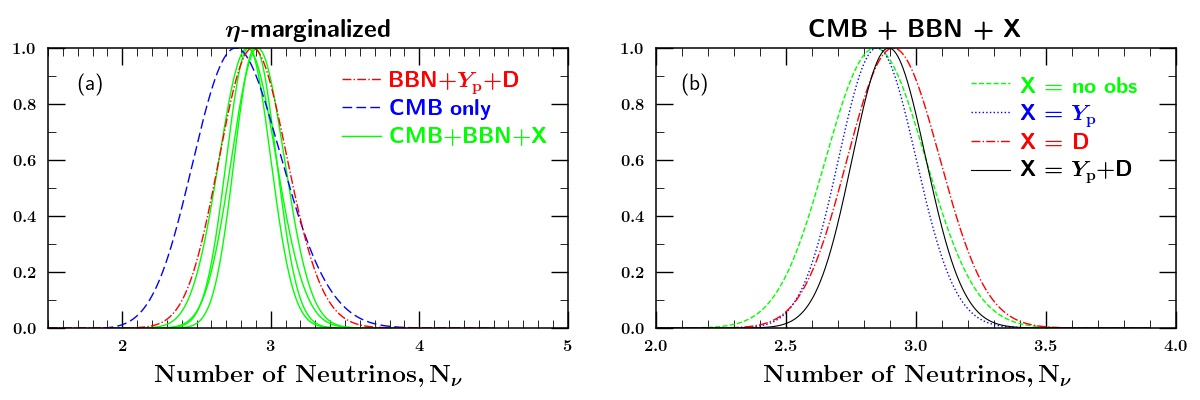
Figure 4: Likelihood distributions for $N_{\nu}$ for BBN and the CMB separately and combined. In all cases shown, the likelihood function has been marginalized over the baryon-to-photon ratio $\eta$. (a) BBN-only, CMB-only, and combined limits. (b) Zoom into BBN+CMB joint limits to highlight results for different combinations of light element abundances. The last three columns of Table 2 summarize these results.

Table 2: The separately marginalized central 68.3% confidence limits and most-likely values on the baryon-to-photon ratio $\eta$ and effective number of neutrinos $N_{\nu}$, using different combinations of observational constraints. The 95.45% upper limits from Eq. (4.4), given that $N_{\nu}>3$, are also shown in the last column.

Constraints Used	mean $\eta_{10}$	peak $\eta_{10}$	mean $N_{\nu}$	peak $N_{\nu}$	$\delta N_{\nu}$
CMB-only	$6.090\pm 0.061$	$6.090^{+0.061}_{-0.062}$	$2.800\pm 0.294$	$2.764^{+0.308}_{-0.282}$	0.513
BBN+$Y_{p}$+D	$5.986\pm 0.161$	$5.980^{+0.163}_{-0.159}$	$2.889\pm 0.229$	$2.878^{+0.232}_{-0.226}$	0.407
CMB+BBN	$6.087\pm 0.061$	$6.088^{+0.061}_{-0.062}$	$2.848\pm 0.190$	$2.843^{+0.192}_{-0.189}$	0.296
CMB+BBN+$Y_{p}$	$6.089\pm 0.053$	$6.089^{+0.054}_{-0.054}$	$2.853\pm 0.148$	$2.850^{+0.149}_{-0.148}$	0.221
CMB+BBN+D	$6.092\pm 0.060$	$6.093^{+0.061}_{-0.060}$	$2.916\pm 0.176$	$2.912^{+0.178}_{-0.175}$	0.303
CMB+BBN+$Y_{p}$+D	$6.088\pm 0.054$	$6.088^{+0.054}_{-0.054}$	$2.898\pm 0.141$	$2.895^{+0.142}_{-0.141}$	0.226

It is also possible to marginalize over $N_{\nu}$ to obtain a likelihood as a function of $\eta$,

$${\cal L}_{\rm NBBN+obs}(\eta)\ \propto\ \int{\cal L}_{\rm NBBN}(\vec{X};\eta,N_{\nu})\ dN_{\nu}\ \prod_{i}{\cal L}_{\rm obs}(X_{i})\ dX_{i}\,.$$ (3.5)

The mean and peak values of $\eta$ from the BBN-only likelihood function is also given in the 2nd row of Table 2.

For the CMB-only results we marginalize the likelihood given in Eq. (3.3) over $\eta$ to obtain the distribution in $N_{\nu}$

$${\mathcal{L}}_{\rm NCMB}(N_{\nu})\ \propto\ \int{\mathcal{L}}_{\rm NCMB}(\eta,N_{\nu})\ d\eta\,.$$ (3.6)

This appears as the dashed blue curve in the left panel of Figure 4, which is entirely consistent with the BBN-only curve and the Standard Model value, though the peak lies slightly below both. The mean and peak values of $N_{\nu}$ from the CMB-only likelihood function is given in the first row of Table 2. Similarly, we can marginalize over $N_{\nu}$ to obtain

$${\mathcal{L}}_{\rm NCMB}(\eta)\ \propto\ \int{\mathcal{L}}_{\rm NCMB}(\eta,N_{\nu})\ dN_{\nu}\,.$$ (3.7)

The mean and peak values of $\eta$ from the CMB-only likelihood function is also given in the first row of Table 2.

Figure 4 shows that the BBN and CMB determinations of $N_{\nu}$ are in excellent agreement with each other, and with the Standard Model value. These three measures are all independent, so their concordance is by no means guaranteed, but to the contrary marks a great success of hot big bang cosmology. Put differently, this agreement tells us that BBN and the CMB are consistent with both the Standard Model ($N_{\nu}=3$) and standard Cosmology ($N_{\nu}^{\rm BBN}=N_{\nu}^{\rm CMB}$), showing no need for new physics within our ability to measure.

It is also remarkable that BBN and the CMB probes $N_{\nu}$ with similar precision. The BBN limits remain slightly tighter, but the improvement of the CMB constraints after Planck has made them closely competitive. The comparable strength in these two measure now offers new ways to probe the early universe, as we now see.

The agreement between the BBN and CMB measures of $N_{\nu}$ invites us to press onward in two ways. (1) We can combine the BBN and CMB limits on $N_{\nu}$, assuming nothing occurs between the two epochs to change this parameter. This analysis appears in §4, and this approach is the one adopted in work to date. (2) We now can also search for, and place limits on, possible differences between $N_{\nu}$ at the BBN and CMB epochs. This approach is novel, and appears in §5.

4 BBN and the CMB Combined: No New Physics After Nucleosynthesis

In this section we combine the BBN and CMB constraints on $N_{\nu}$, and apply the resulting limits to a variety of particle physics and astrophysics examples. The limits we derive here rest on the assumption that $N_{\nu}^{\rm CMB}=N_{\nu}^{\rm BBN}$, that is, there is no change in the cosmic radiation content between the two epochs. This assumption is relaxed in §5. This approach is similar to that used in prior work. Thus our results here for the best fits to $\eta$ and $N_{\nu}$ are an update of our findings in [25], with the only difference being the updates to the $d+d$ reaction rates as explained in §2, as well as an updated primordial helium mass fraction and neutron mean-life.

4.1 BBN+CMB Limits on $N_{\nu}$

Two dimensional joint limits on $(\eta,N_{\nu})$ are obtained using Eq. (3.1) for the BBN-only likelihood and Eq. (3.3) for the CMB-only likelihood function. We can then combine BBN and the CMB to get tighter joint limits on both $\eta$ and $N_{\nu}$. This was first done in [6] and is an extension of the traditional BBN-only approach, e.g., in [62]. The combined likelihood is

$${\cal L}_{\rm NBBN+NCMB+obs}(\eta,N_{\nu})\ \propto\ \int{\cal L}_{\rm NCMB}(\eta,N_{\nu},Y_{p})\ {\cal L}_{\rm NBBN}(\vec{X};\eta,N_{\nu})\ \prod{\cal L}_{\rm obs}(X_{i})\ dX_{i}\ .$$ (4.1)

In cases where ${}^{4}{\rm He}$ observations are used, the $Y_{p}$ marginalization links the BBN and CMB distribution which are both sensitive to this value.

A projection of the likelihood function (4.1) onto the $(\eta,N_{\nu})$ plane is shown by the solid contours in Fig. 5. These are compared with the BBN-only results using Eq. (3.1) and the CMB-only results using Eq. (3.3) in the left and right panels depicted by the dotted contours. We see that the BBN-only constraint shows a significant positive correlation between $\eta$ and $N_{\nu}$. This arises because ${\rm D/H}\propto\eta^{-1.6}N_{\nu}^{0.4}$ and so for fixed $({\rm D/H})_{\rm obs}$, we see the positive correlation $N_{\nu}\propto\eta^{4}$ follows. On the other hand, for the CMB there is very little correlation between $\eta$ and $N_{\nu}$. Both the BBN-only and CMB-only results are consistent with each other, justifying their combined use. Figure 5 displays that BBN provides a slightly better $N_{\nu}$ determination, while the CMB dominates the measurement of $\eta$. This illustrates a BBN-CMB complementarity. As one can see, results are also in excellent agreement with the Standard Model value of $N_{\nu}=3$.

If we marginalize (4.1) over $\eta$, we obtain the distributions over $N_{\nu}$ which appear in Figure 4 for different light element observation combinations. In panel (a) these appear as the solid curves which are zoomed in on in panel (b) which shows the effect of combining the CMB with different BBN+obs choices; this moderately improves on the BBN-only constraints. As one would expect, progressively adding light element observations leads to further modest improvements on the $N_{\nu}$ limit.

Note that the case labeled ‘$X=$ no obs’ corresponds to $\int{\cal L}_{\rm CMB}(\eta,N_{\nu},Y_{p})\ {\cal L}_{BBN}(Y_{p};\eta,N_{\nu})\ d\eta\ dY_{p}$ where we use no astronomical observational data for $Y_{p}$ (or D/H), but through ${\cal L}_{\rm BBN}$ we introduce the BBN theory connection among $Y_{p}$, $\eta$, and $N_{\nu}$. This case gives a noticeably stronger limit on $N_{\nu}$ than those of the CMB only. This demonstrates another aspect of BBN-CMB complementarity, as the tight BBN predictions for $Y_{p}$ alleviate the weaker CMB sensitivity to this parameter.

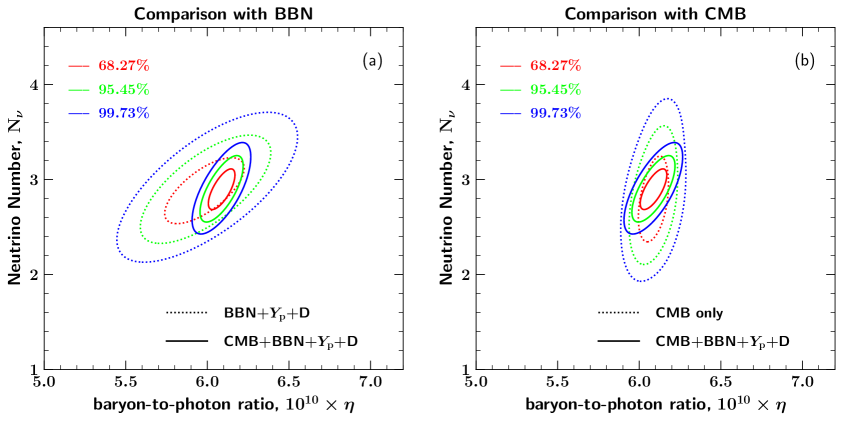
Figure 5: The joint or 2D likelihood ${\cal L}(\eta,N_{\nu})$, assuming these parameters do not change between after BBN. (a) Dashed contours show BBN-only results, while solid contours give combined BBN+CMB results. (b) Contours for the CMB only, and again BBN+CMB combined. Overall, we see that the combined BBN+CMB+obs likelihood combines the virtues of the tight CMB limits on $\eta$ and the stronger BBN limits on $N_{\nu}$.

From Fig. 4 and Table  2 we see that $Y_{p}$ has the stronger impact on the BBN+CMB constraints, but that D/H still has an impact despite playing a lesser role. Improved astronomical $Y_{p}$ measurements, while quite challenging, would thus improve $N_{\nu}$ limits, as we will see below in detail (§6).

Our best limit uses both light elements and the CMB:

$$N_{\nu}=2.898\pm 0.141$$ (4.2)

i.e, the case CMB+BBN+$Y_{p}$+D/H. This gives a 2$\sigma$ upper limit of

$$\Delta N_{\nu}<0.180$$ (4.3)

arising from our two-sided error range about the mean in Eq. (4.2). This result updates that given in Eq. (1.17) by the inclusion of the newly adopted deuterium rates, primordial helium abundance, and neutron mean-life. As one can see, these updates are incremental hopefully indicating the robustness of the limit. We note that this upper limit is almost exactly an order of magnitude tighter than in [62]. For comparison, a scalar particle in equilibrium contributes $\Delta N_{\nu}=4/7=0.57$, so this is ruled out, unless it decouples well before neutrino decoupling [81, 82].

When the best fit value of $N_{\nu}$ is near (or as in Eq. (4.2), below) 3, the resulting limit 2-$\sigma$ upper limit in Eq. (4.3) maybe overly aggressive if we know that there are at least three weakly interacting neutrinos contributing to weak freeze-out. In this case, one can consider a weakened limit by normalizing the likelihood function using only $N_{\nu}\geq 3$ [83] to find the 1-sided limit

$$\frac{\int^{3+\delta N_{\nu}}_{3}{\cal L}(N_{\nu})\ dN_{\nu}}{\int^{\infty}_{3}{\cal L}(N_{\nu})\ dN_{\nu}}=0.9545$$ (4.4)

Thus we demand here that $N_{\nu}>3$ to accommodate the three known light neutrino species. In that case, the last column of Table 2 gives 95.45% CL values for $\delta N_{\nu}$, of which the strongest is

$$\delta N_{\nu}=N_{\nu}-3\ <\ 0.226$$ (4.5)

based on the combination of CMB+BBN+$Y_{p}$+D/H. This one-sided limit is weaker than the corresponding two-sided limit in Eq. (4.3), as expected, but again we see that a fully coupled scalar is ruled out.

The same constraint can be expressed in terms of limits on the speed-up factor

$$\xi=\frac{H(N_{\nu})}{H_{\rm std}}=\sqrt{1+\frac{7(N_{\nu}-3)}{43}}$$ (4.6)

Using Eq. (4.2), and propagating the error, we find the $1\sigma$ range

$$-0.020<\xi-1<0.003$$ (4.7)

and the $2\sigma$ limits

$$\xi-1 < 0.015\ \ \ \ (\mbox{given 2-sided}\ \Delta N_{\nu})$$ (4.8)

$$\xi_{3}-1 < 0.018\ \ \ \ (\mbox{given 1-sided}\ \delta N_{\nu})$$ (4.9)

which are notably larger than the $1\sigma$ upper limit in Eq. (4.7) because the central $N_{\nu}$ value is below 3. Here are throughout, the subscript 3 denotes this case of demanding $N_{\nu}\geq 3$ and thus using the one-sided limit.

Finally, we can express the excess energy density in terms of the critical density, i.e., we can find $\Omega_{X}$ for perturbation $X$. During BBN, the total energy is fully radiation dominated, so that $\rho_{\rm tot}\approx\rho_{\rm rad}$ to high precision, and thus at the start of the BBN epoch (at 2 $\sigma$)

$$\left.\Omega_{X}\right|_{{\rm BBN}} = \frac{\rho_{X}}{\rho_{\rm rad}+\rho_{X}}=\frac{7\Delta N_{\nu}/4}{43/4+7\Delta N_{\nu}/4}<0.028$$ (4.10)

$$\left.\Omega_{X,3}\right|_{{\rm BBN}} = \frac{\rho_{X,3}}{\rho_{\rm rad}+\rho_{X,3}}=\frac{7\delta N_{\nu}/4}{43/4+7\delta N_{\nu}/4}<0.035$$ (4.11)

where $\rho_{\rm rad}$ is the unperturbed radiation density.

By the present day, radiation is a small fraction of the total energy density, for example with $\Omega_{\gamma}h^{2}=2.473\times 10^{-5}$. It is convenient to find the ratio of the density in $X$ to that of photons, which at the start of BBN is $(\rho_{X}/\rho_{\gamma})_{\rm BBN}=g_{X}/2\ (T_{X}/T)^{4}=7/8\ \Delta N_{\nu}$. If $X$ is decoupled by the start of BBN, $T_{X}\propto 1/a$, and so today $(\rho_{X}/\rho_{\gamma})_{0}=(\rho_{X}/\rho_{\gamma})_{\rm BBN}(a_{\rm BBN}T_{\rm BBN}/a_{0}T_{0})^{4}$. Using the conservation of comoving entropy $S=2\pi^{2}/15\ g_{*S}T^{3}a^{3}$, we have $(aT)_{0}/(aT)_{\rm BBN}=(4/11)^{1/3}$ and so

$$\left.\Omega_{X}\right|_{0} = \left(\frac{\rho_{X}}{\rho_{\gamma}}\right)\Omega_{\gamma,0}=\left(\frac{4}{11}\right)^{4/3}\left(\frac{\rho_{X}}{\rho_{\gamma}}\right)_{\rm BBN}\Omega_{\gamma,0}=\frac{7}{8}\left(\frac{4}{11}\right)^{4/3}\Omega_{\gamma,0}\ \Delta N_{\nu}$$ (4.12)

$$= 5.6\times 10^{-6}\ h^{-2}\ \Delta N_{\nu}$$ (4.13)

Thus today we have at $2\sigma$

$$\left.\Omega_{X}\right|_{0} < 1.0\times 10^{-6}h^{-2}$$ (4.14)

$$\left.\Omega_{X,3}\right|_{0} < 1.3\times 10^{-6}\,h^{-2}\ .$$ (4.15)

This limit is much tighter than at BBN simply because the two epochs lie squarely on opposite sides of matter-radiation equality.

4.2 Applications: Constraints on New Physics Prior to BBN

The limits on $N_{\nu}$ (Eq. 4.2) or equivalently the speedup factor (Eq. 4.7) probe physics beyond the Standard Model where the only significant effect on BBN is manifest through the expansion rate, and that $\eta$ is unchanged after BBN. This covers a wide range of new physics possibilities of ongoing interest. Here we illustrate several examples, but we note that this is a necessarily incomplete sample of the large literature on this topic (for reviews see [84, 62, 85, 86]).

4.2.1 Right-Handed Neutrinos

The simplest models generating non-zero neutrino masses require right-handed Standard Model singlet neutrinos. Often these states are quite massive as in the seesaw mechanism, and hence bear no effect on BBN. However, it is possible that light right-handed neutrinos (RHNs) or sterile neutrinos are present and contribute to the energy density at the time of BBN. The standard BBN treatment of neutrinos assumes the Standard Model: three generations of neutrinos with left-handed couplings to the $W$ and $Z$ bosons. If other light ($m_{\nu}\ll 1\,\rm MeV$) neutrinos exist and are populated, these states would of course contribute to $N_{\nu}$.

In the case of Dirac neutrinos, it is obvious from the limit in Eq. (4.5) that three RHNs with full weak-scale interactions (leading to $N_{\nu}=6$) are badly excluded. However, RHN states are not efficiently populated by Standard Model interactions. Nevertheless it is possible, within the limits of either Eqs. (4.3) or (4.5), that three light right-handed states are present provided they decouple from the thermal bath sufficiently early. More precisely, we can translate the limits on $N_{\nu}$ into limits on the RHN temperature at BBN, which can be related to their decoupling temperature and ultimately how strongly they couple to the SM.

For example, for $N_{\nu_{R}}$ new states with mass $m_{\nu_{R}}\ll 1$ MeV and with temperature $T_{\nu_{R}}<T_{\nu_{L}}$, the energy density in relativistic states is

$$\rho_{R}=\rho_{\gamma}+\rho_{e}+\rho_{\nu_{L}}+\rho_{\nu_{R}}=\frac{\pi^{2}}{30}\left(2+\frac{7}{2}+\frac{7}{4}N_{\nu}+\frac{7}{4}N_{\nu_{R}}\left(\frac{T_{\nu_{R}}}{T_{\nu_{L}}}\right)^{4}\right)T^{4}\,,$$ (4.16)

leading to a one-sided limit based on Eq. (4.5) of

$$\frac{T_{\nu_{R}}}{T_{\nu_{L}}}<0.52,$$ (4.17)

when we assume $N_{\nu_{R}}=3$. In order to obtain a right-handed neutrino temperature satisfying (4.17), the RHNs must decouple sufficiently early [81, 82, 87] so that the number of relativistic degrees of freedom at decoupling satisfies

$$g_{dR}>\frac{43}{4}\left(\frac{T_{\nu_{L}}}{T_{\nu_{R}}}\right)^{3}=75\,.$$ (4.18)

This in turn requires that the right-handed neutrinos decouple at a temperature $T_{d\nu_{R}}\gtrsim m_{\tau}$. Using a more precise calculation of the equation of state [88, 89], we find that

$$T_{d\nu_{R}}>1.2~{}{\rm GeV}.$$ (4.19)

Very generically, if we assume that right-handed neutrino decoupling is controlled by contact interactions mediated by a new $Z^{\prime}$ gauge boson then we are able to set a lower bound on the new gauge boson mass

$$M_{Z^{\prime}}\gtrsim\left(\frac{T_{d{\nu_{R}}}}{T_{d{\nu_{L}}}}\right)^{3/4}\left(\frac{43/4}{g_{dR}}\right)^{1/8}\left(\frac{g^{\prime}}{g}\right)M_{Z}\simeq 8.7\left(\frac{g^{\prime}}{g}\right)~{}{\rm TeV}\,,$$ (4.20)

where $g^{\prime}$ is the new gauge coupling, $g$ is the $SU(2)_{L}$ gauge coupling, and we have assumed $T_{d{\nu_{L}}}\sim 2$ MeV [90].

The limit (4.20) is conservative in the sense that we have used the one-sided limit on $N_{\nu}$ requiring $N_{\nu}\geq 3$. A significantly stronger limit on $M_{Z^{\prime}}$ is possible if we employ the more restrictive two-sided limit from Eq. (4.3). In that case, we find $T_{\nu R}/T_{\nu L}<0.49$, which gives $g_{\nu R}>89$. This is only possible if $T_{d{\nu_{R}}}>M_{Z}$, or more accurately from [89], $T_{d{\nu_{R}}}>30$ GeV. This gives a limit $M_{Z^{\prime}}\gtrsim 95$ TeV. Some model-specific limits using the arguments above can be found in Refs. [87, 91, 92, 93, 94, 95]. These limits can be compared to experimental limits on extra $U(1)$ gauge bosons, which are necessarily model-dependent as they depend on how these gauge bosons are coupled to Standard Model particles. For example [96], limits on $Z_{LR}$ in a left-right symmetric model are $M_{Z_{LR}}\gtrsim 1.2$ TeV and mass limits on a $Z^{\prime}$ gauge boson with SM couplings are $M_{Z^{\prime}}>5.1$ TeV.

This generic argument assumes that thermalization occurs through contact interactions below the scale of the gauge boson mass. The derivation of the limit is more complicated at smaller values of the $Z^{\prime}$ gauge coupling where thermal decoupling instead occurs for $T\sim m_{Z^{\prime}}$ through $Z^{\prime}$ decays and inverse decays, while at even smaller couplings out-of-equilibrium freeze-in production can still be constraining. Such effects were worked out for the case of a light, feebly-coupled $U(1)_{B-L}$ gauge boson in [97, 98]; for $1\,\mathrm{MeV}\lesssim m_{Z^{\prime}}\lesssim$ 100 GeV and couplings $g^{\prime}\ll 1$, the resulting contribution of RH neutrinos to $\Delta N_{\nu}$ constitutes the leading probe of the model, together with limits from Supernova 1987A.

Alternatively, the degree to which sterile neutrinos are present in the thermal bath [99, 100, 101, 102, 103, 104] may be constrained by the possible mixing with Standard Model left-handed neutrinos. For example, if $\theta_{s}$ is defined as the mixing angle between active and sterile neutrinos, limits on $\theta_{s}$ can be derived. If $\nu_{1}\approx\cos\theta_{s}\nu_{s}+\sin\theta_{s}\nu_{L}$ and $\nu_{2}\approx\cos\theta_{s}\nu_{L}-\sin\theta_{s}\nu_{s}$ are the two mass eigenstates, the interaction rates for $\nu_{1}$ are similar to those of the active neutrinos, $\nu_{2}$, though suppressed by $\theta_{s}^{2}$ for $\theta_{s}\ll 1$. As in the examples discussed above, $\nu_{1}$ will decouple before $\nu_{2}$ with $T_{d1}\sim T_{d2}\theta_{s}^{-2/3}$ and the limits on $T_{\nu_{R}}$ can be converted into a limit on $\theta_{s}$ [105]. Assuming a single sterile state, $T_{1}/T_{2}<0.69$ requiring $T_{d1}\gtrsim\Lambda_{\rm QCD}$

$$\theta_{s}<\left(\frac{T_{d2}}{T_{d1}}\right)^{3/2}=\left(\frac{2{\rm MeV}}{\Lambda_{\rm QCD}}\right)^{3/2}\lesssim 1.5\times 10^{-3}\,,$$ (4.21)

for $\Lambda_{\rm QCD}=150$ MeV. Other cosmological and astrophysical limits have also been recently discussed [106].

Finally, right-handed neutrino states can allow for the presence of neutrino magnetic moments, whose cosmological effects depends on whether the neutrinos are Dirac or Majorana. In either case, a complete analysis includes changes in neutrino energy spectra and in their cosmic thermodynamics, which are beyond the scope of our analysis; see refs. [107, 108, 109, 110] and references therein.

4.2.2 Dark Radiation

Thermal dark radiation is a frequent ingredient in theories of beyond-the-SM physics. Pseudo-Nambu-Goldstone bosons (pNGBs), for instance, appear in many extensions of the SM, arising from the spontaneous breaking of (for instance) Peccei-Quinn symmetries (axions) [111, 112]; lepton number symmetries (majorons) [113, 114]; or family symmetries (familons) [115]. PNGBs are naturally light and, depending on the reheating temperature and the symmetry-breaking scale, may be thermally populated in the early universe, thereby contributing to dark radiation. However, stellar and supernova cooling bounds on the interactions of these pNGBs with matter typically require that the symmetry breaking scale is sufficiently large to preclude the pNGB from being in equilibrium with the SM plasma at temperatures below the QCD phase transition [116]. Thus in minimal models pNGBs generically do not lead to shifts in $\Delta N_{\rm eff}$ that are large enough to be detected with current sensitivity; however, they represent well-motivated targets for the future. In less minimal models, such as those that contain also a dark matter candidate, e.g. [117], stellar cooling bounds can be relaxed and substantially larger contributions to $N_{\mathrm{eff}}$ are possible.

More generally, multi-state hidden sectors offer many avenues to address the origin of dark matter (DM), whether DM is a thermal or non-thermal relic. DM may be produced by a thermal freeze-out process from a dark radiation bath, stabilized through a dark number asymmetry similar to the baryon asymmetry, or through a more complicated interplay of equilibrium and non-equilibrium mechanisms; see e.g. [118] for an overview of recent work. In such hidden sector scenarios, dark matter is produced out of a dark thermal bath, which carries a sizeable amount of entropy. The simplest way to accommodate this entropy is to sequester it in dark radiation, which requires the existence of a light degree of freedom in the hidden sector spectrum. Otherwise the lightest hidden sector state(s) must decay into the SM in the early universe, which imposes severe restrictions on the abundance and lifetime of the decaying particle(s). A relativistic relic contributing to dark radiation thus represents a generic (though not universal) component of dark sector model building.

Thermal hidden sectors in the early universe are also motivated by approaches to the hierarchy problem. The Twin Higgs mechanism introduces a mirror or ‘twin’ copy of the SM, related to the SM by a discrete symmetry that ensures a cancellation between the contributions of SM and twin particles to the Higgs mass parameter [119]. Exact cancellations require the introduction of twin photons and twin neutrinos, which can all contribute to dark radiation. Given the Higgs portal interactions inherent between twin and SM particles, twin particles are in thermal equilibrium with the SM in the early universe until temperatures of $\mathcal{O}(\mathrm{GeV})$, and thus mirror Twin Higgs models require a period of late asymmetric reheating in order to dilute the dark radiation to levels allowed by current constraints [120, 121]. Another approach to the hierarchy problem is furnished by NNaturalness [122], which postulates a large number $N$ of copies of the SM that differ by the value of the Higgs mass-squared parameter, with Higgs-reheaton couplings arranged such that the sector with the smallest non-zero Higgs vacuum expectation value is preferentially populated in the early universe. The massless species from the additional sectors, populated at much lower temperatures than the SM, then contribute to dark radiation.

In a self-interacting dark sector, the dark radiation may have cosmologically relevant interactions with other dark species. In some theories these interactions can keep the dark radiation in internal kinetic equilibrium, so that it acts as a perfect fluid, rather than a free-streaming relic, during recombination. Both fluid and free-streaming dark radiation affect BBN in the same way, through the contribution of their (homogeneous) energy density to the Hubble rate, and therefore both are subject to BBN constraints on $N_{\nu}$. However, the imprint of fluid dark radiation on the power spectrum of the CMB anisotropies has a different phase than in the free-streaming case appropriate for SM neutrinos, and the contribution of fluid dark radiation must be quantified by the observable $N_{\mathrm{fluid}}$ rather than $N_{\mathrm{eff}}$ [123, 124]. CMB constraints on $N_{\mathrm{fluid}}$ are typically weaker by a factor of 2-3 than the corresponding CMB constraints on $N_{\mathrm{eff}}$ [125, 126]. Theories with fluid dark radiation are still subject to the BBN-only constraints on $N_{\mathrm{eff}}$ derived in Section 3.

The energy density carried in thermal dark radiation depends on its temperature $T_{DR}$, which will in general differ from that of the SM, as well as the number of its degrees of freedom $g_{*HS}$. Dark radiation contributes to the energy density in relativistic species as

$$\rho_{\rm DR}=g_{*\rm HS}(T_{\rm DR})\frac{\pi^{2}}{30}T_{\rm DR}^{4}.$$ (4.22)

In describing multi-state hidden sectors, we need to account for a possible time-varying $g_{*\rm HS}$ as hidden sector species may become nonrelativistic and deposit their entropy into the remaining dark radiation. Denoting the value of $g_{*\rm HS}$ immediately prior to BBN as $g_{*\rm HS}^{\rm IR}$, from Eq. (1.11) the contribution to $\Delta N_{\nu}$ is

$$\Delta N_{\nu}=\frac{4}{7}g_{*\rm HS}^{\rm IR}\left(\frac{T_{\rm DR}}{T_{\nu}}\right)^{4}=2.2g_{*\rm HS}^{\rm IR}\left(\frac{T_{\rm DR}}{T_{\gamma}}\right)^{4},$$ (4.23)

where in the last equality we have used $T_{\nu}=(4/11)^{1/3}T_{\gamma}$. Assuming entropy conservation, we can rewrite this expression in terms of the HS and SM temperatures and effective entropic degrees of freedom $g_{*S}(T)$ at some earlier time as

$$\Delta N_{\nu}=2.2g_{*HS}^{IR}\left(\frac{T_{DR}^{UV}}{T_{\gamma}^{UV}}\right)^{4}\left(\frac{43/4}{g_{*S,SM}(T_{\gamma}^{UV})}\right)^{4/3}\left(\frac{g_{*S,HS}(T_{DR}^{UV})}{g_{*S,HS}(T_{DR}^{IR})}\right)^{4/3}.$$ (4.24)

Thus if the HS and the SM were in thermal equilibrium at some common UV temperature $T_{\gamma}^{\rm UV}=T_{\rm DR}^{\rm UV}=T_{*}$, the resulting shift in $N_{\nu}$ depends only on the evolution of the numbers of degrees of freedom in both sectors following decoupling:

$$\Delta N_{\nu}=2.2g_{*HS}^{IR}\left(\frac{43/4}{g_{*S,\rm SM}(T_{*})}\right)^{4/3}\left(\frac{g_{*S,\rm HS}(T_{*})}{g_{*S,\rm HS}(T_{\rm DR}^{\rm IR})}\right)^{4/3}.$$ (4.25)

The one-sided upper bound from Eq. (4.5) requiring $\delta N_{\nu}<0.226$ thus allows two relativistic degrees of freedom to have been in equilibrium with the SM at early times (i.e., taking $g_{*S,\rm SM}=g_{*,\rm SM}=106.75$). This bound is stringent enough to preclude nontrivial evolution in $g_{*\rm HS}$ once the HS has decoupled from the SM: e.g., putting $g_{*S,\rm HS}(T_{*})=2$ and $g_{*\rm HS}^{\rm IR}=g_{*S,\rm HS}^{\rm IR}=1$ in Eq. (4.25) results in $\Delta N_{\nu}=0.26$. Of course, if there are additional BSM species in the thermal plasma at early times that deposit their entropy preferentially into the SM, the temperature of the dark radiation is then further suppressed relative to that of the SM, and more degrees of freedom can be accommodated. Dark sectors may also be populated out of equilibrium with the SM in the early universe, e.g. via asymmetric reheating [127], in which case the temperature ratio between the photons and the dark radiation is a free parameter and $g_{*\rm HS}$ may be substantially larger.

4.2.3 Stochastic Gravitational Wave Background

A gravitational wave background is a generic prediction of inflation models. After inflation, processes in the early universe such as phase transitions or the evolution of cosmic string networks can also source stochastic gravitational wave backgrounds; see, e.g., ref. [128]. Regardless of its origin, the energy density in gravitational waves laid down before BBN acts as radiation and thus its impact on BBN is completely captured by our $N_{\nu}$ analysis. Gravitational waves with adiabatic initial conditions leave the same imprint on the CMB as free-streaming dark radiation, and for this case the limit on the present-day energy density in gravitational waves is that in Eq. (4.15), namely

$$\Omega_{\rm GW,0}\,h^{2}<1.3\times 10^{-6}\ \ \ (f\gtrsim 2\times 10^{-11}\ {\rm Hz})$$ (4.26)

where we impose $N_{\nu}>3$. This is similar to recent “indirect” limits based on BBN and the CMB and quoted by the LIGO and VIRGO collaborations [129, 130]. Other recent limits using the CMB, often in concert with BBN, are in refs. [131, 132, 133, 134]. Gravitational waves with non-adiabatic initial conditions give rise to a different CMB signature and can be more tightly constrained; results appear in ref. [135].

The BBN constraint on stochastic gravitational waves applies to frequencies above a cutoff $f\gtrsim f_{\rm BBN}$. This restriction on the frequency range arises because the BBN limit applies to modes that are within the horizon at the start of BBN, so that the comoving wavenumber is larger than the inverse of the comoving Hubble length $d_{\rm H,com}=1/aH$ at the time, i.e., $k_{\rm BBN}>a_{\rm BBN}H_{\rm BBN}$ [136]. Setting $T_{\rm BBN}=1\,\rm MeV$ gives $z_{\rm BBN}=5.9\times 10^{9}$, and then $f_{\rm BBN}=k_{\rm BBN}/2\pi=1.8\times 10^{-11}\ \rm Hz$. A similar argument gives a CMB frequency cutoff $f_{\rm CMB}\gtrsim 10^{-16}\ \rm Hz$. This means that while the limit in Eq. (4.26) applies for the frequency range indicated, if there is a gravitational wave component with $f_{\rm CMB}<f<f_{\rm BBN}$, this will contribute to $N_{\nu}^{\rm CMB}$ but not to $N_{\nu}^{\rm BBN}$. This would lead to an effective time variation in $N_{\nu}$, which is the subject of §5.

4.2.4 Vacuum Energy: Tracker Solutions

A scalar field $\phi$ present during BBN contributes vacuum energy that affects the cosmic expansion rate [84]. In particular, quintessence models for dark energy often have tracker solutions, in which the scalar field providing the dark energy behaves as the dominant cosmic mass-energy component until late times when the field drives cosmic acceleration today [84, 137, 138, 139, 140]. Thus, $\rho_{\phi}$ effectively acts as a subdominant component of radiation during BBN, and is amenable to our analysis.

The limit applies during BBN, where the energy density must obey Eq. (4.11), i.e.,

$$\left.\Omega_{\phi}\right|_{\rm BBN}<0.035$$ (4.27)

Note that for this result is valid when the tracker field behaves like radiation throughout BBN and CMB, with the same fraction of the radiation density over all of this time.

For a potential $V(\phi)=M_{\rm Pl}^{4}e^{-\lambda\phi/M_{\rm Pl}}$, the coupling is constrained to be $\lambda=2M_{\rm Pl}/\sqrt{\Omega_{\phi}}>11$.

4.2.5 Changing Fundamental Couplings

Though there is no intrinsic reason that fundamental couplings are in fact constant, there are many constraints which limit their time variation. For a review see: [141]. Some of the strongest limits are derived from BBN since the temporal baseline is essentially the age of the Universe. In most cases, the limits derived from BBN can be traced to their effect on the freeze-out of the weak interactions which determine the neutron-to-proton ratio. That is, any new physics which alters either Eqs. (1.2) or (1.3), will affect $T_{f}$ and hence $n/p$. Very simply, we have

$$\frac{\Delta(n/p)}{(n/p)}=\frac{\Delta m}{T_{f}}\frac{\Delta T_{f}}{T_{f}}\,,$$ (4.28)

which induces a change in the light elements, most notably $Y_{p}\approx 2(n/p)/(1+(n/p))$. This is the basis for the limits on $N_{\nu}$ and more generally $\xi$ as these directly affect $H$ in Eq. (1.3).

A variation in the fine-structure constant, $\alpha$, however affects the neutron-proton mass difference (which then affects $n/p$). The neutron-proton mass difference receives both weak and electromagnetic contributions

$$\Delta m=a\,\alpha\,\Lambda+b(h_{d}-h_{u})\,v\,,$$ (4.29)

where the electromagnetic contribution is $a\,\alpha\,\Lambda=-0.76\ \rm MeV$ and is proportional to the QCD scale $\Lambda$, while the weak contribution is $b({h_{d}}-{h_{u}})\,v=2.05\ \rm MeV$, where $h_{d,u}$ are the Yukawa couplings to the $u$ and $d$ quarks and $v$ is the Higgs expectation value [142]. Therefore a change in $\alpha$ directly affects $\Delta m$ and Eq. (4.28) is modified

$$\frac{\Delta(n/p)}{(n/p)}=\frac{\Delta m}{T_{f}}\left(\frac{\Delta T_{f}}{T_{f}}-\frac{\Delta^{2}m}{\Delta m}\right)\,,$$ (4.30)

where $\Delta^{2}m$ is the change in $\Delta m$. This leads to a variation in $Y_{p}$

$$\frac{\Delta Y_{p}}{Y_{p}}=\frac{\Delta m/T_{f}}{1+(n/p)}\left(\frac{\Delta T_{f}}{T_{f}}-\frac{\Delta^{2}m}{\Delta m}\right)\approx 1.3\frac{\Delta^{2}m}{\Delta m}\,,$$ (4.31)

where the last inequality assumes $T_{f}\approx 0.84$ MeV. Thus the bounds on $Y_{p}$ constrain $\Delta^{2}m$ and hence $\alpha$ [143, 144, 145, 146, 147].

From Eq. (4.29), $\Delta^{2}m=-0.76\Delta\alpha/\alpha\ \rm MeV$ and using the observational uncertainty in $Y_{p}$ from Eq. (1.5), we have

$$\frac{\Delta\alpha}{\alpha}\lesssim 0.018\,.$$ (4.32)

Though it probes a different cosmological epoch, Planck constraints on variations in $\alpha$ from the CMB are now tighter than that from BBN. Intermediate Planck results [148] give $\Delta\alpha/\alpha=(3.6\pm 3.7)\times 10^{-3}$ or $\Delta\alpha/\alpha<0.007$ at 1 $\sigma$, somewhat stronger than the limit in Eq. (4.32). However, in many theories which allow for a variation in $\alpha$, that variation is accompanied by variations in other fundamental parameters [144, 149, 150, 151, 152, 153] affecting not only the neutron-proton mass difference, but also the deuterium binding energy and other quantities relevant to BBN [144, 146, 154, 155, 156, 157, 158, 159, 160, 161, 162]. These considerations are more model dependent, but generally provide limits which are roughly two orders of magnitude stronger than (4.32).

While variations in $\alpha$ and other couplings affect the weak interaction rates in Eq. (1.2), a variation in the gravitational constant directly affects Eq. (1.3) and the limit on $G_{\rm N}$ can easily be cast in the form of a limit on $N_{\nu}$. Of course any consideration of a variation in $G_{\rm N}$, implicitly assumes the constancy of some masses, e.g., the proton mass, so that it is the variation of the gravitational coupling $G_{\rm N}m_{p}^{2}$ which is constrained.

From Eq. (1.3), we see that $H^{2}\propto G_{\rm N}$, and we thus have $\Delta G_{\rm N}/G_{\rm N}=\xi^{2}-1=(7/43)(N_{\nu}-3)$. Using $N_{\nu}=2.898\pm 0.141$ we find the 1 $\sigma$ range

$$-0.040<\frac{\Delta G_{\rm N}}{G_{\rm N}}<0.006\ \ .$$ (4.33)

The asymmetry in the bounds is traced to the central value of $N_{\nu}$ lying sightly below 3. More conservatively we have at 2 $\sigma$

$$-.062<\left(\frac{\Delta G_{\rm N}}{G_{\rm N}}\right) < 0.029$$ (4.34)

$$0<\left(\frac{\Delta G_{\rm N}}{G_{\rm N}}\right)_{3} < 0.037\,$$ (4.35)

which is similar to recent work [163]. If we parameterize the variation as $G_{\rm N}\sim t^{-x}$ [164, 165, 166, 167, 168, 163], the 2 sigma limits become $-0.002<x<0.0007$ and $x<0.0009$, respectively. These corresponds to a limit $-5.1\times 10^{-14}~{}{\rm yr}^{-1}<{\dot{G}}_{\rm N}/G_{\rm N}<1.1\times 10^{-13}~{}{\rm yr}^{-1}$ and $-6.5\times 10^{-14}~{}{\rm yr}^{-1}<{\dot{G}}_{\rm N}/G_{\rm N}<0$ (for the 2-sided and 1-sided limits), which is slightly better than the strongest limit from lunar-laser-ranging [169] giving ${\dot{G}}_{\rm N}/G_{\rm N}<2.2\times 10^{-13}$ yr^-1.

As a variation in $G_{\rm N}$ effectively implies a non-minimal theory of gravity, we can translate the bounds on the variation into bounds on parameters in specific non-minimal models. For example, in Brans-Dicke gravity, the variation in $G_{\rm N}$ can be translated in a limit on the coupling $\omega$ ($\omega\to\infty$ corresponds to the limit of Einstein gravity) which is bound by BBN [170, 171, 172, 173, 167]. Our 2-sided and 1-sided limits on $\omega$ are $\omega>270$ and $>230$ respectively. These are weaker than bounds imposed by the CMB which are of order 2000 [174, 175, 176, 177]. Both cosmological limits are weaker than the limits obtained by Doppler tracking of the Cassini spacecraft [178] which gives $\omega>15000$ (2 $\sigma$) [179].

4.2.6 Primordial Magnetism

Primordial magnetic fields could be created in the very early universe, e.g., during inflation. The fields would thus be present during BBN. Jedamzik et al [180] showed that magnetic field modes are damped at scales much below the horizon at neutrino decoupling. As Cheng et al [181] note, this means that magnetic fields during BBN are well-approximated as a uniform perturbation to the energy density. The energy density $\rho_{B}=B^{2}/8\pi\propto a^{-4}$ scales as radiation because the field obeys $B\propto a^{-2}$ due to flux conservation.

Magnetic fields during BBN not only add to the energy density through $\rho_{B}$. They also perturb the $e^{\pm}$ density of states, and thus (1) boost the the energy density and pressure due to pairs, and (2) change the $n\rightarrow p$ interconversion rates. For field strengths of interest, the effect of $\rho_{B}$ dominates the perturbation to BBN, and thus is amenable to our treatment; see refs. [181, 182, 183] for detailed analysis.

Taking the approximation of the field’s energy density as the dominant perturbation, we have $B^{2}/8\pi<\Delta N_{\nu}\ \rho_{1\nu}$. At the beginning of BBN, this corresponds to $B(1\ {\rm MeV})<2.6\times 10^{13}\ \rm Gauss$; today this would be $B_{0}<2.8\ \rm\mu G$.

5 Searching for new physics between the BBN and CMB epochs

Up until now, we have assumed that the values of $\eta$ and $N_{\nu}$ remained unchanged between the time of BBN and CMB decoupling. However, it is possible that new physics is responsible for a change in these quantities and therefore, we now drop the assumption that one or both of $N_{\nu}$ and $\eta$ are the same for the BBN and CMB epochs. This probes possible evolution in these quantities. The data allow us to probe scenarios where only one of $\eta$ or $N_{\nu}$ change, or where both change. As we will see, these correspond to different physical scenarios. For example, a stable particle becoming non-relativistic after BBN would change $N_{\nu}$ only, while decays or annihilations of some beyond the Standard Model particles into Standard Model particles can change both $\eta$ and $N_{\nu}$.

The baryon-to-photon ratio is intimately related to the comoving entropy of relativistic species

$$S_{\rm com}=a^{3}\,s=\frac{2\pi^{2}}{45}\ g_{*,S}\ (aT)^{3}\ \ .$$ (5.1)

where $s$ is the entropy density and $a$ is the cosmological scale factor. Here $g_{*,S}=\sum_{\rm boson}g_{b}(T_{b}/T)^{3}+7/8\ \sum_{\rm fermion}g_{f}(T_{f}/T)^{3}$ is the usual effective number of entropic degrees of freedom, summed over relativistic species. For constant $g_{*,S}$, we see that $S_{\rm com}\propto(aT)^{3}$, and thus the photon temperature $T\propto 1/a$ when $S_{\rm com}$ is conserved. Note also that the baryon density (assuming baryon number conservation) scales as $n_{B}\propto 1/a^{3}$, and the photon number density $n_{\gamma}\propto T^{3}$, the baryon-to-photon ratio can be normalized to its present value $\eta_{0}$

$$\eta=\frac{n_{\rm B}}{n_{\gamma}}=\eta_{0}\left(\frac{a_{0}T_{0}}{aT}\right)^{3}\,.$$ (5.2)

Thus a change in entropy and a change in the product $aT$ can be related to $\eta$

$$\eta=\frac{2\pi^{2}g_{*,S}a_{0}^{3}T_{0}^{3}\eta_{0}}{45S_{\rm com}}\ \ .$$ (5.3)

Thus we have $\eta\propto(g_{*,S}/S_{\rm com})$, and is it clear that entropy production—changing the comoving entropy $S_{\rm com}$—leads to changes in $\eta$.

We note that variations in $\eta$ can in some cases be linked to changes in $N_{\nu}$. This is because the cosmic entropy is dominated by that in relativistic species via the second law of thermodynamics: $T\,dS_{\rm com}=d(\rho_{\rm rel}a^{3})+p_{\rm rel}d(a^{3})=a^{-1}d(\rho_{\rm rel}a^{4})$, where $\rho_{\rm rel}$ and $p_{\rm rel}$ correspond to the energy density and pressure of relativistic species. Thus entropy change $dS_{\rm com}\neq 0$ in relativistic species also implies a change in $\rho a^{4}$, which can be parameterized by $N_{\nu}$.

We therefore treat $\eta^{\rm BBN}$ and $\eta^{\rm CMB}$ as distinct, as we do for $N_{\nu}^{\rm BBN}$ and $N_{\nu}^{\rm CMB}$. To probe their joint distribution, we convolve over the light element abundances

$${\cal L}(N_{\nu}^{\rm BBN},\eta^{\rm BBN},N_{\nu}^{\rm CMB},\eta^{\rm CMB})$$

$$\propto \int{\cal L}_{\rm NCMB}(\eta^{\rm CMB},N_{\nu}^{\rm CMB},Y_{p})\ {\cal L}_{\rm NBBN}(\vec{X};\eta^{\rm BBN},N_{\nu}^{\rm BBN})\prod_{i}{\cal L}_{\rm obs}(X_{i})\ dX_{i}\ \ .$$

This serves to link the CMB and BBN distributions via their dependence on $Y_{p}$.

We continue to assume the light elements did not change after BBN, so that the their observations are valid to apply for both BBN and the CMB. In particular, by using low-redshift astronomical observations $Y_{p,\rm obs}$ from extragalactic HII regions (Eq. 1.5), we are implicitly assuming that there is not any cosmologically important (i.e., pre-stellar) nucleosynthesis between BBN and recombination:

$$Y_{p}^{\rm BBN}=Y_{p}^{\rm CMB}=Y_{p,\rm obs}\ \ .$$ (5.5)

There are several ways to proceed to understand the constraints on this 4-dimensional space. We first examine possible changes in $N_{\nu}$ alone.

5.1 Limits on $\mathrm{N_{\nu}}$ Evolution

Our evaluations of $N_{\nu}$ in Fig. 4 include both CMB-only and BBN-only analyses, which give independent measures. We see that the two measures are remarkably consistent, $|N_{\nu}^{\rm CMB}-N_{\nu}^{\rm BBN}|$ is roughly one third of the half-width of the distributions. We already see that the CMB and BBN show no need for a change in $N$ between the epochs, a theme we will see repeated. Thus it is reasonable to combine them as we have in the previous section; here we examine the extent to which they are allowed to differ. Processes which may change the value of $N_{\nu}$ between BBN and CMB decoupling include decays of non-relativistic particles to relativistic ones which would increase $N_{\nu}$, or some relatively light particle (say of order 1 keV), becoming non-relativistic, thereby decreasing $N_{\nu}$.

We marginalize over the two $\eta^{i}$ to compare the neutrino numbers and produce the likelihood

$${\cal L}(N_{\nu}^{\rm BBN},N_{\nu}^{\rm CMB})\ \propto\ \int{\cal L}(N_{\nu}^{\rm BBN},\eta^{\rm BBN},N_{\nu}^{\rm CMB},\eta^{\rm CMB})\ d\eta^{\rm BBN}\ d\eta^{\rm CMB}\,.$$ (5.6)

In the marginalization, we adopt the least restrictive assumption regarding $\eta^{i}$, i.e., we do not demand that the two $\eta^{i}$ are related, and allow them to differ. This is appropriate for scenarios where a change in $\eta$ is possible.

Results for Eq. (5.6) appear in Fig. 6. Panel (a) shows the joint constraints in the $(N_{\nu}^{\rm BBN},N_{\nu}^{\rm CMB})$ plane. We we see that the $1\sigma$ contour includes the Standard Model case of $(3,3)$, while the best fit likelihood peak is slightly below 3 in both variables. The dotted diagonal line shows $N_{\nu}^{\rm CMB}=N_{\nu}^{\rm BBN}$, which almost perfectly bisects the contours, and the best-fit point (shown by the yellow dot) is very close to this line. Indeed, the nearly circular contours also show that the BBN and CMB constraints have very similar spreads (and that the $Y_{p}$ convolution does not introduce much correlation). These results reaffirm that the Standard Model works very well: neither BBN nor the CMB provide any significant evidence for new physics. Moreover, the remarkable agreement between the independent values of $N_{\nu}$ measured by the CMB and BBN also shows that there is no preference for a change in $N_{\nu}$ between the two epochs. Thus we proceed to use these results to limit changes in $N_{\nu}$.

Panel (b) of Fig. 6 explores the allowed range in the

$$DN_{\nu}\equiv N_{\nu}^{\rm CMB}-N_{\nu}^{\rm BBN}$$ (5.7)

difference. Here for each value of $DN_{\nu}$, we marginalize the distribution in panel (a) to obtain the likelihood, ${\cal L}(DN_{\nu})$ shown in panel (b). We see that the peak is very near zero (the Standard Model value is shown by the vertical dotted line), indicating that there is no preference for $N_{\nu}$ evolving between these two epochs. The best fit being $DN_{\nu}=-0.064\pm 0.342$. Note that the uncertainty here is related to the uncertainties obtained in the previous section for BBN-alone and CMB-alone, and in this case as one might expect, the combined uncertainty in $DN_{\nu}$ is larger than either of the two individually. The vertical dot-dashed lines give the 95% 2-sided limits on $DN_{\nu}$. We see that while the $2\sigma$ limits on the difference in $N_{\nu}$ do not allow 1 full neutrino species, but could allow a net gain or loss of a fully-coupled scalar.

Panel (c) of Fig. 6 is similar to panel (b), but now requires that both the BBN and CMB values have $N_{\nu}>3$. This amounts to marginalizing over fixed values of $DN_{\nu}$ within the top right corner outlined by dotted lines in panel (a). The distribution in panel (c) peaks sharply at $DN_{\nu}\simeq 0$, indicating consistency with the Standard Model. Vertical dot-dashed lines show 95% one-sided limits on the difference, which we see are quite strong: positive values have $DN_{\nu}<0.312$, while negative values have $-DN_{\nu}<0.350$. We see that the difference is too small to accommodate a full scalar appearing or disappearing between the two epochs.

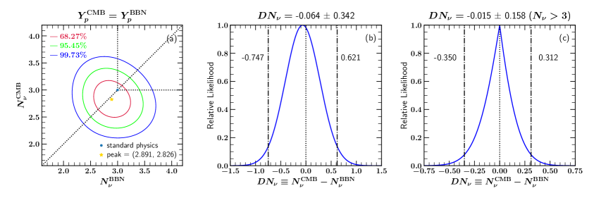
Figure 6: CMB vs BBN independent determinations of $N_{\nu}$. We marginalize over $\eta$ in both epochs separately as shown in Eq. (5.6), after convolving with light elements as in Eqs. (5) and (5.5). We adopt the Aver et al $Y_{p}$ [28] as in Eq. (1.5). Panel (a) compares the two measures, showing that the best-fit point is quite close to the diagonal $N_{\nu}^{\rm CMB}=N_{\nu}^{\rm BBN}$ line, and within 1 sigma of the Standard Cosmology result at $(3,3)$. We note that the BBN and CMB constraints are quite comparable to each other. Panel (b) shows the distribution of the difference $DN_{\nu}\equiv N_{\nu}^{\rm CMB}-N_{\nu}^{\rm BBN}$, which peaks nearly at the Standard Cosmology value $\Delta N_{\nu}=0$. The vertical dot-dashed lines show the 95% two-sided limit. Panel (c) is similar to panel (b) but requiring $N_{\nu}\geq 3$. Vertical lines give the 95% one-sided limits. Overall we see that our results are in excellent agreement with the Standard Cosmology expectations, and thus we place limits on nonstandard alternatives where $\Delta N_{\nu}\neq 0$.

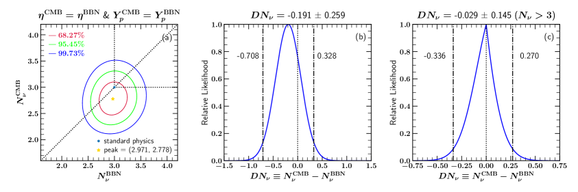
Figure 7: CMB vs BBN determinations of $N_{\nu}$. Similar to Fig. 6 but additionally demanding $\eta^{\rm CMB}=\eta^{\rm BBN}$.

In principle, there could be scenarios where $N_{\nu}$ changes between BBN and the CMB but $\eta$ does not. Therefore it is appropriate to consider a likelihood function constrained by $\eta^{\rm BBN}=\eta^{\rm CMB}$ which gives

$${\cal L}(N_{\nu}^{\rm BBN},N_{\nu}^{\rm CMB})\ \propto\ \int{\cal L}(N_{\nu}^{\rm BBN},\eta,\ N_{\nu}^{\rm CMB},\eta)\ ;\ \ d\eta\qquad\eta=\eta^{\rm BBN}=\eta^{\rm CMB}$$ (5.8)

where the integrand is given by Eq. (5). This likelihood distribution is expected to give stronger limits on the change in $N_{\nu}$ if the BBN- and CMB-preferred $\eta$ values are similar. Results for this case appear in Fig. 7. We see that the results for each panel are quite similar to those from the corresponding part of Fig. 6, but as expected the limits are tighter. Again all three panels show results fully consistent with the Standard Model. In panel (b), the $\Delta N_{\nu}$ is slightly shifted to negative values, but by less than $1\sigma$.

These limits place new constraints on many kinds of models for physics in the early universe; we now discuss a few examples.

Early Dark Energy models.

A change in $N_{\nu}$ between BBN and the CMB occurs in Early Dark Energy models [184]. For the case of an oscillating scalar field in a potential which is approximately quartic about the minimum, the oscillations act like radiation with an equation of state $w=1/3$. Using best-fit values, the dark energy component acts as radiation for scale factors $a>a_{\rm c}\approx 1.9\times 10^{-4}$ or $z_{\rm c}\approx 5300$, close to the epoch of matter-radiation equality when $a_{\rm eq}=\Omega_{\rm r,0}/\Omega_{\rm m,0}\approx 1/3400$. Thus, during recombination this component will act as radiation, adding to $N_{\nu}$. At $z_{c}$, the model requires a best-fit $f_{\rm EDE}=\Omega_{\phi}(a_{c})=0.044$, assuming $\Omega_{\rm tot}=1$. Compared to the ordinary radiation density, we have $\rho_{\phi}(a_{c})/\rho_{r}(a_{c})=f_{\rm EDE}(1+a_{c}/a_{\rm eq})$. We can write $\rho_{\phi}/\rho_{r}\approx g_{1\nu}\,DN_{\nu}^{\rm EDE}/(2+3g_{1\nu})$, with $g_{1\nu}=7/4\ (4/11)^{4/3}$. We thus cast the early dark energy perturbation during the CMB as

$$DN_{\nu}^{\rm EDE}\approx f_{\rm EDE}\left(1+\frac{a_{c}}{a_{\rm eq}}\right)\left[3+\frac{8}{7}\left(\frac{11}{4}\right)^{4/3}\right]=0.53\ \ ,$$ (5.9)

an increase of about half of an equivalent neutrino species at recombination. Comparing to our results from this section, we see that this is allowed when $N_{\nu}$ is free, but is not allowed (at 2 $\sigma$) when $N_{\nu}>3$ in Fig. 6. Furthermore, from Fig. 7, we see that when $\eta$ is held fixed between BBN and CMB decoupling, $DN_{\nu}<0.33$ putting still more pressure on this model. Indeed as we will see in the next subsection, to attain $DN_{\nu}^{\rm EDE}$ as large as that in Eq. (5.9), would require an increase in $\eta$ between the BBN and CMB epochs. This model–or more precisely, this choice of $(f_{\rm EDE},a_{c},w)$–is thus at best marginally allowed from our viewpoint. Moreover, this example shows that there is a role for constraints of the type we have presented. Other early dark energy models with different potentials and hence different equations of state parameters $w$ will also be constrained by BBN + CMB limits, but these cannot be parameterized by $N_{\nu}$ and so would require dedicated study.

Relativistic relic becoming nonrelativistic.

A BSM particle $\chi$ that contributes to $N_{\nu}$ during BBN may become nonrelativistic prior to the formation of the CMB. In this case the number of effective relativistic degrees of freedom will decrease between the two epochs, leaving $\eta$ unaffected. The contribution of such a free-streaming relativistic relic to $N_{\mathrm{eff}}$ during BBN can be written in a very general way as

$$\rho_{\chi}|_{BBN}=\left(\frac{a_{\mathrm{nr}}}{a_{\mathrm{eq}}}\right)f_{\rm DM}\times\left(\frac{\Omega_{\rm cdm}}{\Omega_{\rm m}}\right)\rho_{SM}|_{BBN},$$ (5.10)

where $a_{\mathrm{nr}}$ is the scale factor when the relic becomes nonrelativistic and $a_{\mathrm{eq}}$ is the scale factor at matter-radiation equality, with $a_{\mathrm{nr}}<a_{\mathrm{eq}}$, $f_{\rm DM}<1$ is the fraction of dark matter contributed by the relic after it becomes nonrelativistic, and $\Omega_{\rm cdm},\,\Omega_{\rm m}$ are the fractions of critical density in cold dark matter and total matter (CDM $+$ baryons). Here we have assumed only that the evolution of the energy density of $\chi$ can be well-approximated as redshifting like radiation for $a<a_{\mathrm{nr}}$ and matter for $a>a_{\mathrm{nr}}$. Specific models of warm dark matter, such as sterile neutrinos, will relate $f_{\rm DM}$ and $a_{\mathrm{nr}}$ to the mass and production mechanism of the hot relic $\chi$. Given this expression for the energy density for the relativistic relic, the corresponding shift in $N_{\nu}$ is

$$-DN_{\nu}=6.2\left(\frac{a_{\mathrm{nr}}}{a_{\mathrm{eq}}}\right)f_{\rm DM},$$

where we have used the results of Ref. [8] for cosmic parameters. Imposing the one-sided constraint $-DN_{\nu}<0.336$, we thus obtain

$$\left(\frac{a_{\mathrm{nr}}}{a_{\mathrm{eq}}}\right)f_{\rm DM}<0.054.$$ (5.11)

For fractions $f_{\rm DM}$ near unity, this result constrains relics becoming nonrelativistic at sufficiently early times that the assumption of a constant value of $N_{\nu}$ at the CMB epoch is consistent.

This dark radiation disappearance limit depends on two key properties of the relic: (i) the scale $a_{\mathrm{nr}}$ at which it becomes nonrelativistic, and (ii) the fraction $f_{\rm DM}$ of dark matter that the relic represents after it becomes nonrelativistic. These two properties are also exactly the same quantities that are important for understanding the potential impact of the hot relic on structure formation, which lets us make some general observations about $DN_{\nu}$ limits compared to those arising from measurements of the Lyman-$\alpha$ forest. The free-streaming horizon

$$\lambda_{FS}=\int_{t_{0}}^{t_{f}}\frac{v}{a}dt\approx\frac{1}{a_{\mathrm{nr}}H_{nr}}\left[1+\ln\left(a_{\mathrm{eq}}/a_{\mathrm{nr}}\right)\right]$$ (5.12)

is a useful estimate for the maximum scale on which a hot relic can suppress the growth of density perturbations in the early universe. While Lyman-$\alpha$ constraints on warm relics require specifying the model-dependent phase space distribution of the relic, when $f_{\rm DM}=1$ (and again assuming a phase-space distribution characterized by a single momentum scale), it is possible to extract a conservative and model-insensitive requirement that $\lambda_{FS}\lesssim 0.1$ Mpc in order to match current observations [186]. Approximating the Hubble rate as piecewise power laws in the scale factor $a$ lets us write

$$\lambda_{FS}\approx\frac{1}{H_{0}}\sqrt{\frac{\Omega_{R}\Omega_{\Lambda}}{\Omega_{M}^{2}}}\frac{a_{\mathrm{nr}}}{a_{\mathrm{eq}}}\left[1+\ln\left(a_{\mathrm{eq}}/a_{\mathrm{nr}}\right)\right].$$ (5.13)

For $f_{\rm DM}=1$ the $DN_{\nu}$ limit on $a_{\mathrm{nr}}/a_{\mathrm{eq}}$ in eq. (5.11) translates into the weaker constraint $\lambda_{FS}\lesssim 24$ Mpc using eq. (5.13). Thus for models of light relics, independent of the detailed microphysics in a given model, the present $DN_{\nu}$ limit is meaningful but less constraining than the current Lyman-$\alpha$ limits (for more model-specific statements see [186, 187, 188, 189]).

Late equilibration with neutrinos.

BSM physics that has relevant interactions with the SM neutrinos can come into equilibrium with the SM neutrinos after BBN and subsequently become nonrelativistic, depositing their entropy into the neutrino bath [190, 191, 192, 193]. In such scenarios the effective number of neutrinos increases between BBN and the CMB, while leaving $\eta$ and $Y_{p}$ unaffected. The one-sided constraint $DN_{\nu}<0.270$ allows for a single relativistic degree of freedom to equilibrate with the SM neutrinos provided its temperature before BBN was no more than $0.6T_{\gamma}$. Late equilibration with a particle species with more than one degree of freedom cannot be accommodated.

Inflationary dark vectors decaying to neutrinos.

Dark vector bosons produced through inflationary fluctuations can decay to SM neutrinos if they couple to the $B-L$ current, or similarly to the current for one of the other anomaly-free but non-flavor-universal global $U(1)$ symmetries of the SM, $L_{i}-L_{j}$ or $B-3L_{i}$ [194]. When this decay occurs between neutrino decoupling and recombination, it gives rise to a shift in $N_{\nu}$ while leaving $\eta$ unaffected. The vector boson’s mass controls the timing of its decay, but not the size of the resulting shift in $N_{\nu}$; instead, this shift depends quadratically on the (unknown) Hubble scale during inflation and inversely on the vector boson’s coupling to neutrinos [194]. The constraints on this scenario from the limit $DN_{\nu}<0.270$ are slightly more stringent than those shown in [194], which used a CMB+LSS $\Delta N_{\mathrm{eff}}$ constraint of $\Delta N_{\mathrm{eff}}<0.28$.

5.2 Limits on the Evolution of the Baryon-to-Photon Ratio

In this section, we place limits on changes in the baryon-to-photon ratio between BBN and CMB decoupling. As shown in Eq. (5.3), changes in comoving entropy lead to changes in $\eta$. In the standard picture $e^{\pm}$ pair annihilation transfers entropy to photons during BBN, and BBN calculations include these effects. Here we look for changes in $\eta$ beyond this, and between the two epochs.

Nonstandard scenarios with entropy change include particle creation or destruction, e.g., by out-of-equilibrium decays. As noted in the discussion surrounding Eq. (5.3), entropy change typically also changes $N_{\nu}$, and such cases are treated in the next subsection. Indeed, it is challenging to try to construct physically motivated scenarios that change $\eta$ while holding $N_{\nu}$ fixed. Nevertheless, for completeness we show results for such scenarios here.

For the most conservative limits, we marginalize separately over $N_{\nu}^{\rm BBN}$ and $N_{\nu}^{\rm CMB}$:

$${\cal L}(\eta^{\rm BBN},\eta^{\rm CMB})=\int{\cal L}(N_{\nu}^{\rm BBN},\eta^{\rm BBN},N_{\nu}^{\rm CMB},\eta^{\rm CMB})\ dN_{\nu}^{\rm BBN}\ dN_{\nu}^{\rm CMB}\ \ .$$ (5.14)

Note that the 4-D integrand imposes $Y_{p}^{\rm CMB}=Y_{p}^{\rm BBN}$ via Eq. (5). Results appear in Fig. 8. We see that the peak values of $\eta^{\rm CMB}$ and $\eta^{\rm BBN}$ are indeed quite close to each other, less than $1\sigma$ apart. They thus are close to dotted diagonal line giving the Standard Model case $\eta^{\rm CMB}=\eta^{\rm BBN}$. This is a manifestation of the BBN-CMB concordance that stands as a success of the hot big bang theory. The plot also makes clear the well-known result that the CMB measurement of $\eta$ is substantially tighter than that from BBN. Finally, we see that there is not a significant correlation between the two $\eta$ values, despite using a common $Y_{p}$ constraint. This is because $Y_{p}$ does not play an important role in setting $\eta^{\rm BBN}$.

We denote the change in baryon-to-photon ratio as

$$D\eta=\eta^{\rm CMB}-\eta^{\rm BBN}\ \ ,$$ (5.15)

and for convenience we also use $D\eta_{10}=10^{10}D\eta$. Panel (b) of Fig. 8 shows the distribution of this difference. Each value of $D\eta_{10}$ corresponds to a diagonal in panel (a), and we marginalize over this diagonal to find the value at each point in panel (b). We see that $D\eta_{10}$ peaks close to the Standard Model $D\eta=0$ value, with a slight preference for positive values. As a result, the limits on negative $D\eta$ are stronger than those for positive values.

We saw in Eq. (5.3) that $\eta\propto g_{*S}/S_{\rm com}$: an increase in the entropy of the baryon-photon plasma leads to a decrease in $\eta$. With this in mind, we note that the 1-sided limit on a decrease $D\eta_{10}<0$,

$$\left.D\eta_{10}\right|_{\rm min}=-0.287$$ (5.16)

at $2\sigma$ (the 2-sided limits are shown in Fig. 8). Given the mean $\eta_{10}\sim 6$, this means only a $\sim 5\%$ decrease is allowed.

We have also examined possible changes in $\eta$ in the case where we require $N_{\nu}>3$ at both BBN and CMB epochs. These results appear in Fig. 9, where the main lesson is that the consistency with the Standard Model is even better, with the peaks in both panels even closer to $D\eta=0$. The one-sided limit on the decrease $D\eta_{10}<0$ now becomes

$$\left.D\eta_{10}\right|_{\rm min,N>3}=-0.251$$ (5.17)

at $2\sigma$ (the 2-sided limits are shown in Fig. 9), now allowing only a $\sim 4\%$ difference. We see that very little change is allowed in the baryon-to-photon ratio, and thus in entropy, between BBN and the CMB.

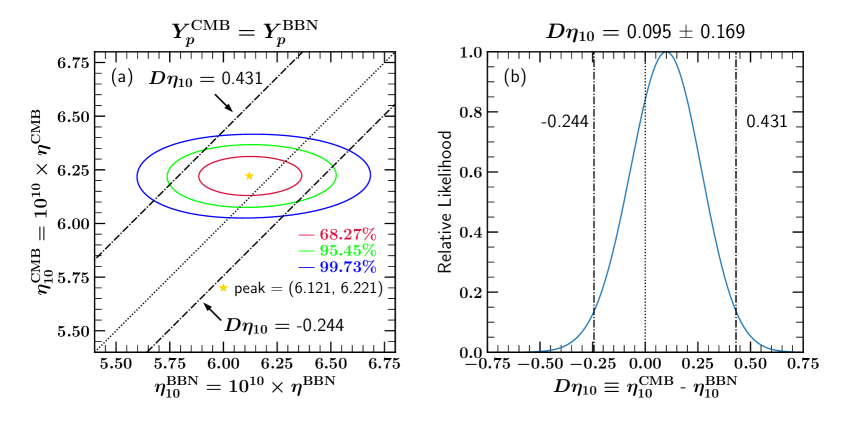
Figure 8: A comparison of the independent BBN and CMB measures of $10^{10}\eta$, marginalizing separately over all $N_{\nu}$ values but holding $Y_{p}$ fixed as in Fig. 6. Panel (a) shows $\eta^{\rm CMB}$ vs $\eta^{\rm BBN}$ likelihood contours. We see that the best-fit point lies within $1\sigma$ of the Standard Cosmology $\eta^{\rm CMB}=\eta^{\rm BBN}$ shown by the dotted line. We also see that $\eta^{\rm CMB}$ constraints are significantly tighter. Panel (b) shows the distribution for the difference $D\eta=\eta^{\rm CMB}-\eta^{\rm BBN}$. The dot-dashed lines show the the two-sided 95% CL limits, and these also appear as the dot-dashed diagonal lines in (a). We see the peak lies near the Standard Cosmology $D\eta=0$ value, and that there are rather tight limits on deviations away from this value.

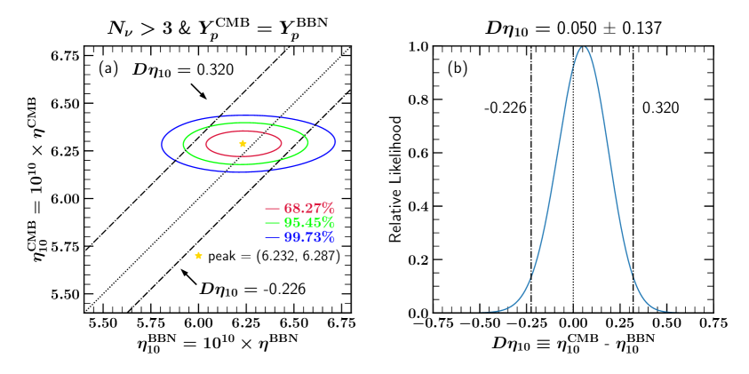
Figure 9: Similar to Fig. 8, but requiring $N>3$ for both the CMB and BBN.

5.3 Limits on Evolution of Both $\eta$ and $N_{\nu}$

We now relax the assumption that only one of $\eta$ and $N_{\nu}$ varies, and we allow for both to change between nucleosynthesis and recombination. Examples where this situation can occur would be entropy-producing scenarios such as annihilations or decays into photons.

For our most conservative case, we do not require $Y_{p}^{\rm CMB}=Y_{p}^{\rm BBN}$. Rather, we use equation (3.1) for ${\cal L}_{\rm NBBN+obs}(\eta,N_{\nu})$, and marginalize over $Y_{p}$ to find

$${\mathcal{L}}_{\rm NCMB}(\eta,N_{\nu})\ \propto\ \int{\mathcal{L}}_{\rm NCMB}(\eta,N_{\nu},Y_{p})\ dY_{p}\,.$$ (5.18)

We then calculate the likelihoods for the differences $D\eta=\eta^{\rm CMB}-\eta^{\rm BBN}$ and $DN_{\nu}=N_{\nu}^{\rm CMB}-N_{\nu}^{\rm BBN}$:

$${\mathcal{L}}_{\rm NCMB+NBBN+obs}(D\eta,DN_{\nu})\ \propto\ \int{\mathcal{L}}_{\rm NCMB}(\eta+D\eta,N_{\nu}+DN_{\nu}){\cal L}_{\rm NBBN+obs}(\eta,N_{\nu})\ d\eta\,dN_{\nu}\ .$$ (5.19)

This convolution takes the 4D distribution in Eq. (5) down to a 2D distribution by focusing on the differences in $\eta$ and $N_{\nu}$.

If we do require that the BBN and CMB $Y_{p}$ values are the same, as in Eq. (5.5), then the convolution

$${\cal L}_{\rm NBBN+NCMB+obs}(D\eta,DN_{\nu})\ \propto\ \int{\cal L}_{\rm NCMB}(\eta+D\eta,N_{\nu}+DN_{\nu},Y_{p})\ {\cal L}_{\rm NBBN}(\vec{X};\eta,N_{\nu})\ \prod{\cal L}_{\rm obs}(X_{i})\ dX_{i}\ d\eta\ dN_{\nu}\$$ (5.20)

gives the likelihood distribution for the change in these parameters.

Fig. 10 shows the allowed changes in $\eta$ and $N_{\nu}$ for both cases. Remarkably, but at this point not surprisingly in panel (a) and (b) the maximum likelihood is close to $(0,0)$. That is, even with this greater freedom, we again see that the Standard Model gives an excellent fit, and the data do not show a need for variation between the two epochs. We also see a positive correlation between $D\eta$ and $DN_{\nu}$. This reflects the fact shown in Fig. 5 that BBN alone (and to lesser extent, the CMB alone) has a positive $(\eta,N_{\nu})$ correlation. Figure 11 is similar to Fig. 10, but now allowing only $N_{\nu}>3$ for both BBN and the CMB. We see in Fig. 10 that the regions with $DN_{\nu}<3$ allow for larger deviations between the two epochs. Thus when we exclude these, the result is mostly a narrowing of the allowed $N_{\nu}$ range.

Figures 10 and 11 also generalize some of our earlier results. The $N_{\nu}$ change for $\eta^{\rm CMB}=\eta^{\rm BBN}$ corresponds to a vertical line at $D\eta=0$; this is what is shown in Fig. 7.

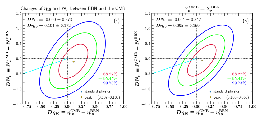
Figure 10: Allowed variation in both $\eta$ and $N_{\nu}$ between BBN and the CMB, assuming $Y_{p}$ is the same in both epochs in panel (b). The cyan lines are for the scenario described in eqs. (5.21-5.22), for the case of $f_{\gamma}=1$.

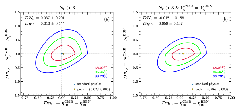
Figure 11: Similar to Fig. 10, but now requiring $N>3$.

One immediate application of these constraints is a species that decays out of equilibrium in the epoch between BBN and recombination, which can inject sufficient energy and entropy into the SM radiation bath to alter both $N_{\mathrm{eff}}$ and $\eta$. Related work has focused on particle decays [195, 196, 197, 198]. We illustrate the impact of this varying-$\eta$, varying-$N_{\nu}$ analysis with a general example where a decaying particle injects energy density $\Delta\varepsilon$ into the photon bath after the conclusion of BBN and before the formation of the CMB. We consider the case where all of this energy is deposited into photons at redshifts $z\gtrsim\mathrm{few}\,\times 10^{6}$, so that it can be simply parameterized by a shift in the photon temperature [199]. In this redshift range constraints on $DN_{\nu}$ and $D\eta$ provide a leading probe of energy injection in the early universe, while spectral distortions become more powerful at lower redshifts [200].

To leading order in the fractional energy injection $\Delta\varepsilon/\rho_{\gamma}^{CMB}$, the shift in $\eta$ and $N_{\nu}$ resulting from such an energy injection can be written

$$D\eta \approx \eta^{CMB}\left[-\frac{3}{4}\frac{\Delta\varepsilon}{\rho_{\gamma}^{CMB}}\right]$$ (5.21)

$$DN_{\nu} \approx N_{\nu}^{BBN}\left[-\frac{\Delta\varepsilon}{\rho_{\gamma}^{CMB}}\right],$$ (5.22)

where $\Delta\varepsilon$ parameterizes the net energy deposited into photons after the conclusion of BBN, such that $\rho_{\gamma}^{CMB}=\rho_{\gamma}^{BBN}(a_{BBN}/a_{CMB})^{4}+\Delta\varepsilon$.

We can now constrain the fractional energy release $\Delta\varepsilon/\rho_{\gamma}^{\rm CMB}$ using the 2-D joint constraints from from Fig. 10. As $\Delta\varepsilon/\rho_{\gamma}^{\rm CMB}$ varies from $0$ and up, the constraints in eqs. (5.21-5.22) describe a line in the $(D\eta,DN_{\nu})$ plane, taking $N_{\nu}^{\rm BBN}$ and $\eta^{\rm CMB}$ as fixed. This line appears in Fig. 10(a), and intersects the $2\sigma$ contour at $(D\eta,DN_{\nu})=(-0.28,-0.18)$. These correspond respectively to limits $\Delta\varepsilon/\rho_{\gamma}^{\rm CMB}<(0.061,0.062)$ which are almost equal, and so the $D\eta$ constraint drives the limit

$$\frac{\Delta\varepsilon}{\rho_{\gamma}^{\rm CMB}}<0.061\ \ .$$ (5.23)

Here we adopted the central value for $\eta_{\rm CMB}$, but the uncertainty on this quantity is $<1\%$, and so our limit is essentially unchanged. Note that in this case, the analysis shown in Fig. 11 does not apply, because it assumes $N_{\nu}\geq 3$ for both the BBN and CMB epochs. But even in the presence of SM neutrinos, in this example the heating of photons relative to neutrinos will lead to $T_{\nu}/T_{\gamma}<(4/11)^{1/3}$, which would show up in CMB analyses as $N_{\nu}^{\rm CMB}<3$.

In a case where the decaying species deposits a fraction $f_{\gamma}$ of its energy into photons while the remaining fraction $1-f_{\gamma}$ is deposited into neutrinos, the resulting shifts in $\eta$ and $N_{\nu}$ become, again to leading order in $\Delta\varepsilon/\rho_{\gamma}^{CMB}$,

$$DN_{\nu} \approx N_{\nu}^{BBN}\left[\frac{1-f_{\gamma}}{c_{\nu}N_{\nu}^{BBN}}-f_{\gamma}\right]\frac{\Delta\varepsilon}{\rho_{\gamma}^{CMB}}$$ (5.24)

$$D\eta \approx \eta^{CMB}f_{\gamma}\left[-\frac{3}{4}\frac{\Delta\varepsilon}{\rho_{\gamma}^{CMB}}\right],$$ (5.25)

where $c_{\nu}=\frac{7}{8}\left(\frac{4}{11}\right)^{4/3}$. Using $N_{\nu}^{\rm BBN}=3$, the bracketed coefficient in eq. (5.24) goes from $-1$ to $+1.47$ as $f_{\gamma}$ decreases from 1 to 0. There is a finely-tuned value of $f_{\gamma,0}=(1+N_{\nu}^{\rm BBN}c_{\nu})^{-1}=0.595$ for which the energy of the decaying particle is shared between photons and neutrinos in a ratio that exactly replicates that predicted by the standard cosmology, resulting in $DN_{\nu}=0$, while $\eta$ still decreases. Thus, the $DN_{\nu}$ variation is largest and positive for $f_{\gamma}=1$, vanishes for $f_{\gamma}=f_{\gamma,0}$ and reverses sign for $f_{\gamma}<f_{\gamma,0}$. Also, for all $f_{\gamma}$ the $DN_{\nu}/N_{\nu}-D\eta/\eta$ correlation is still linear, but the slope is generally shallower than for $f_{\gamma}=1$, becoming negative for $f_{\gamma}<f_{\gamma,0}$. For $f_{\gamma}=0.5$, we find that the $D\eta$ constraint in Fig. 10(a) is stronger, and with $D\eta/\eta^{\rm CMB}<-0.36$ gives $\Delta\varepsilon/\rho_{\gamma}^{\rm CMB}<0.096$, almost a factor of 2 weaker than the result in eq. (5.23).

The photon bath can also experience a net entropy increase if it comes into equilibrium with a feebly-coupled dark sector after BBN [190, 192]. This late equilibration can be naturally realized in theories where a light (sub-MeV) species mediates interactions between photons and one or more SM singlet fields. Concrete models that realize late equilibration with the photon plasma are however subject to a number of stringent constraints, particularly from stellar cooling [192].

6 The Expected Impact of Future Observations: CMB-S4, Precision ⁴He Observations and the Hunt for Neutrino Heating

We look forward to a bright future in which the constraints we have presented will become stronger. For the microwave background, CMB Stage-4 (CMB-S4) will be the next generation ground-based CMB experiment. CMB-S4 is expected to improve the CMB precision at small angular scales, reducing uncertainties at high multipoles in CMB anisotropy power spectra. Such improvement will result in a better CMB measurement of $\sigma(N_{\nu})$. On the BBN side, the $Y_{p}$ uncertainties from astronomical observations currently dominate the size of BBN $\sigma(N_{\nu})$. Therefore, we also look forward to future improvements on the precision of primordial helium observations to provide BBN-only $N_{\nu}$ determination that can compete with the expected CMB-S4 results.

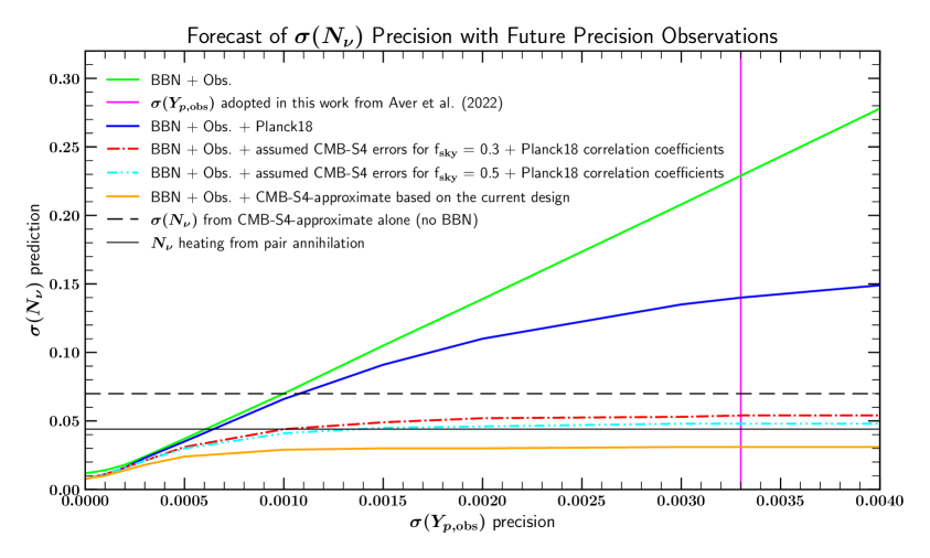
Figure 12: Impact on the precision of $N_{\nu}$ due to future improvements in astronomical ${}^{4}{\rm He}$ measurement precision. Curves show the $\sigma(Y_{p,\rm obs})$ impact on $\sigma(N_{\nu})$ for the cases of (a) BBN+Obs., which in green shows a nearly linear scaling down for most of the range, and of (b) BBN+Obs.+CMB, where the shallower and nonlinear responses reflect the contribution of past and future CMB constraints on $N_{\nu}$ (in blue and orange respectively). The vertical line for the current $\sigma(Y_{p,\rm obs})$, the horizontal dashed line for the expected $\sigma(N_{\nu})$ from the CMB-S4-approximate case alone, and the horizontal solid line for the impact of neutrino heating are three auxiliary lines for reference. We see it is very promising to probe the neutrino heating effect by combining current BBN constraints with the future CMB-S4 data.

Figure 12 shows forecasts for the uncertainty in $N_{\nu}$ in response to improvements in astronomical measurements of $Y_{p}$. The different curves show the expected $\sigma(N_{\nu})$ given the observed $\sigma(Y_{p})$ error budget, for different combinations of BBN with CMB measurements past and future. For BBN alone (shown in green), we see that the trend is linear over most of the domain; this reflects the fact that for BBN only, $Y_{p}$ dominates the $N_{\nu}$ inference. We see that for BBN alone, to begin to see the effects of neutrino heating (Eq. 1.8) with $\sigma(N_{\nu})<0.044$ (shown by the solid-black line) requires very precise helium determinations: $\sigma(Y_{p})<0.0006$.

Figure 12 also highlights the dramatic improvements when BBN and CMB measurements are combined (the solid-blue curve). We see that adding the Planck 2018 information dramatically improves the $N_{\nu}$ sensitivity for $Y_{p}$ measurements at or somewhat below the current levels. At the current $\sigma(Y_{p})=0.0033$, we see that BBN+CMB combination improves the $\sigma(N_{\nu})$ by about a factor of 2. Note that the BBN-only and CMB-only errors are comparable, so the effect is not just one of averaging, but rather the combination breaks degeneracies and so is quite powerful. There remains significant improvement down to $\sigma(Y_{p})\simeq 0.0012$, but to reach the neutrino heating still requires similar ${}^{4}{\rm He}$ precision to the BBN-only case.

Looking forward to CMB-S4, we find the BBN+CMB-S4 combination should be very powerful. The CMB-S4 constraints are sensitive to the fraction $f_{\rm sky}$ of the sky observed. We will use $f_{\rm sky}^{\rm S4}=0.3$ as a baseline for CMB-S4, but a larger sky coverage would tighten the limit. We assume in our toy model that the CMB-S4 likelihood is a multivariate Gaussian distribution and has $\sigma(N_{\rm eff}^{\rm S4})=(0.09,0.08)$ and $\sigma(Y_{p}^{\rm S4})=(0.0055,0.0047)$ for $f_{\rm sky}^{\rm S4}=(0.3,0.5)$. These values are approximately inferred from the Figure 28 of the CMB-S4 science book [202], which provides forecasts for $\sigma(N_{\rm eff}^{\rm S4})$ and $\sigma(Y_{p}^{\rm S4})$ as functions of sky fraction. We also use the correlations of these three parameters from the same Planck MCMC chains for $N_{\nu}\neq 3$ adopted in the previous sections. Both cases are shown in Figure 12 respectively as the dashdotted-red and the dashdotdotted-cyan curves. We again find that combining BBN+CMB reduces the uncertainty budget substantially, so that even at the present $Y_{p}$ sensitivity, $\sigma(N_{\nu})\approx 0.05$, very close to the neutrino heating limit, and substantially better than the CMB alone. To push below the neutrino heating limit is somewhat less demanding of ${}^{4}{\rm He}$ observations, albeit challenging, requiring $\sigma(Y_{p})<0.001$ when $f_{\rm sky}^{\rm S4}=0.3$.

To further improve the joint $\sigma(N_{\nu})$ sensitivity, the correlation between $N_{\rm eff}^{\rm S4}$ and $Y_{p}^{\rm S4}$ plays a crucial role. This correlation has impact on how the CMB likelihood convolves with the BBN likelihood on the $N_{\nu}$-$Y_{p}$ plane, determining the spread of the combined $N_{\nu}$ likelihood. In our toy model, we found that if the correlation coefficient $\rho^{\rm\ S4}_{(N_{\rm eff},Y_{p})}\sim-0.9$ at $f_{\rm sky}^{\rm S4}=0.3$, i.e. highly anti-correlation between $N_{\rm eff}^{\rm S4}$ and $Y_{p}^{\rm S4}$, we can get a joint $\sigma(N_{\nu})\sim 0.03$ ($\sim 1$ % uncertainty) even with the present $Y_{p}$ sensitivity. This agrees with forecasts in refs. [202, 205, 36]. We note that attaining this precision requires that the real CMB-S4 reaches the key entries assumed in our toy model–not only the relevant parameter uncertainties, but also the strong $N_{\rm eff}-Y_{p}$ anticorrelation.

The orange curve in Figure 12 shows the expected joint $\sigma(N_{\nu})$ at different $Y_{p}$ precision using a CMB-S4 example likelihood forecast calculated and kindly provided by Benjamin Wallisch based on refs. [206, 207, 208, 204, 209]. This particular forecast, labeled as “S4-approximate” in the figure, is based on a set of internal-linear-combination noise curves derived from a version of the current design and a simple foreground model, and provides an approximation of what CMB-S4 is currently thought to look like. Given that the key inputs of this likelihood are $\sigma(N_{\rm eff}^{\rm S4})=0.071$, $\sigma(Y_{p}^{\rm S4})=0.0045$, and $\rho^{\rm\ S4}_{(N_{\rm eff},Y_{p})}=-0.848$, our BBN+CMB-S4 forecast displays the joint $\sigma(N_{\nu})\simeq 0.03$ for the most range of $\sigma(Y_{p})>0.001$ including the current observed ${}^{4}{\rm He}$ uncertainty. Thus, it is very promising to probe the neutrino heating effect by combining current BBN constraints with the future CMB-S4 data.

An expected CMB-S4 precision $\sigma(N_{\nu})\simeq 0.03$ also reaches the Standard Model lower limit $\Delta N_{\nu}>0.027$ for a scalar that was ever thermally populated (Eq. (1.13) with $g_{X,\rm eff}=1$). This will make CMB-S4 a powerful probe not only of Standard Model physics but also of departures from it. Importantly, BBN plays a critical role here: the CMB-only “S4-approximate” constraint only reaches $\sigma(N_{\nu})\simeq 0.07$ if the BBN relation $Y_{p}(\eta)$ is not used (long-dashed horizontal dashed line in Fig. 12).

We also note that this forecasted S4 CMB-only limit $\sigma(N_{\nu})\simeq 0.07$ would still be challenging to match with BBN alone. To catch up with such a sensitivity as well in the BBN-only case, future ⁴He astronomical observations need to reach $\sigma(Y_{p})\simeq 0.001$. The lesson is that BBN and the CMB are most powerful when working together.

Finally, CMB-S4 should also improve the CMB measure of ${}^{4}{\rm He}$ to $\sigma(Y_{p}^{\rm CMB})\simeq 0.0045$. While this will improve the precision by a factor of $\sim 4$ from the Planck value, it is still larger then the current errors $\sigma(Y_{p}^{\rm obs})=0.0033$ from astronomical observations. Even so, the independent and clean $Y_{p}^{\rm CMB}$ measurement will offer an important consistency check on $Y_{p,{\rm obs}}$ and its systematics. Along similar lines, another independent cross-check would be measurement of $Y_{p}$ from helium signatures in the kinetic Sunyaev-Zel’dovich effect [210].

7 Discussion and Conclusions

BBN constraints on $N_{\nu}$ have long stood as a prototypical example of cosmological probes of new physics. Now CMB measurements have reached similar precision. We find that these independent BBN and CMB measures of $N_{\nu}$ are consistent with each other and with the Standard Model; this represents a non-trivial success of hot big bang cosmology. We have explored the consequences of using BBN and the CMB jointly and separately to look for new physics. First, we updated the joint BBN+CMB constraints for the case where $N_{\nu}$ does not change between these two epochs. The resulting limits in Eqs. (4.3 - 4.5) tighten the constraints new physics in the early universe, which we illustrated with several examples.

Second, advances in the BBN and CMB precision now also allow us to meaningfully probe changes in $N_{\nu}$ and $\eta$ between these two epochs. We find the the current data is consistent with the Standard Model, with only modest departures allowed. We applied our limits to early dark energy models for the $H_{0}$ tension, finding that BBN+CMB constraints can be significant. We also placed bounds on changes in $\eta$ that limit entropy production between BBN and the CMB.

It bears repeating that the limits we have set are valid when an effective value for $N_{\nu}$ adequately captures the effect of new physics. Our results apply to situations where the only important perturbation adds a radiation-like component to the cosmic energy density, and where there is no additional effects on structure growth as probed by the CMB. Moreover, our work requires that $N_{\nu}$ takes a constant value throughout the BBN epoch, and similarly for the CMB, though possibly with a different value. Cases where our treatment is inadequate require dedicated analyses; these include perturbations with density that does not evolve as radiation such as early matter domination, or where interactions with the baryon-photon plasma can affect reaction rates. And finally, we have assumed the primordial lithium problem does not have a new physics solution [47]; were that to be the case, a bespoke analysis is again required.

To further sharpen BBN and CMB constraints on new physics, we look forward to new precision results in nuclear experiments, nuclear theory, astronomical observations, and CMB measurements. BBN predictions for deuterium still have larger errors than D/H observations, due to the uncertainties in major deuterium destruction rates $d(d,n)\mbox{${}^{3}{\rm He}$}$, $d(d,p)t$, and $d(p,\gamma)\mbox{${}^{3}{\rm He}$}$ (listed by their contribution to the predicted D/H uncertainty). We point out that measurements of the $d+d$ reaction are the most urgently needed, and better theoretical understanding of these rates would also be illuminating. Also, if BBN theory errors can be reduced via new cross section measurements, D/H can become a stronger probe of $N_{\nu}$. Improvements in nuclear theory would be useful as well, particularly for deuterium rates: ref. [43] use nuclear theory in deriving thermonuclear rates, and find D/H abundances that are discrepant with the results of the empirical approach adopted here and in ref. [42].

Improved astronomical measurements of the light elements can also advance the field. For D/H, it may be challenging to improve the already small error in the mean, but to continue to test for systematics, it remains critical to find additional good systems across as wide as possible a range of redshift and metallicity. As we have shown, improvements in astronomical ${}^{4}{\rm He}$ observations will sharpen $N_{\nu}^{\rm BBN}$ and thus sharpen the comparison with $N_{\nu}^{\rm CMB}$. And of course, an unambiguous solution to the lithium problem remains outstanding (but see ref. [47]).

Finally, the upcoming CMB-S4 will improve $N_{\rm eff}$ measurements. The projected CMB-S4-alone precision $\sigma(N_{\rm eff})\simeq 0.07$ will then likely provide a stronger probe of $N_{\nu}$ than BBN. To catch up with such CMB-S4 precision on the BBN side, future primordial ⁴He observations must reach $\sigma(Y_{p,{\rm obs}})\simeq 0.001$, $\sim 1/3$ of the current (already-excellent) uncertainty. Moreover, the predicted BBN+CMB-S4 joint precision $\sigma(N_{\nu})\simeq 0.03$ bring in reach new regimes in both conventional and exotic physics. We will be able to discriminate for the first time the difference $N_{\rm eff}-3=0.044$ for the effect of neutrino heating. And this sensitivity to $N_{\nu}$ can reveal the effects of new particles that were in thermal equilibrium at temperatures above the masses of all Standard Model particles. We look forward to this view of the early Universe coming into focus.

References

- [1] R.A. Alpher and R.C. Herman, Remarks on the Evolution of the Expanding Universe, Phys. Rev. 75 (1949) 1089.
- [2] T.P. Walker, G. Steigman, D.N. Schramm, K.A. Olive and H.-S. Kang, Primordial Nucleosynthesis Redux, ApJS 376 (1991) 51.
- [3] K.A. Olive, G. Steigman and T.P. Walker, Primordial nucleosynthesis: theory and observations, Physics Reports 333 (2000) 389 [astro-ph/9905320].
- [4] G. Steigman, Primordial Nucleosynthesis in the Precision Cosmology Era, Annual Review of Nuclear and Particle Science 57 (2007) 463 [0712.1100].
- [5] F. Iocco, G. Mangano, G. Miele, O. Pisanti and P.D. Serpico, Primordial nucleosynthesis: From precision cosmology to fundamental physics, Physics Reports 472 (2009) 1 [0809.0631].
- [6] R.H. Cyburt, B.D. Fields, K.A. Olive and T.-H. Yeh, Big bang nucleosynthesis: Present status, Rev. Mod. Phys. 88 (2016) 015004.
- [7] C. Pitrou, A. Coc, J.-P. Uzan and E. Vangioni, Precision big bang nucleosynthesis with improved Helium-4 predictions, Physics Reports 754 (2018) 1 [1801.08023].
- [8] Planck collaboration, Planck 2018 results. VI. Cosmological parameters, Astron. Astrophys. 641 (2020) A6 [1807.06209].
- [9] F. Hoyle and R.J. Tayler, The Mystery of the Cosmic Helium Abundance, Nature 203 (1964) 1108.
- [10] V.F. Shvartsman, Density of relict particles with zero rest mass in the universe, Pisma Zh. Eksp. Teor. Fiz. 9 (1969) 315.
- [11] P.J.E. Peebles, Physical cosmology, Princeton University Press (1971).
- [12] G. Steigman, D.N. Schramm and J.E. Gunn, Cosmological limits to the number of massive leptons, Physics Letters B 66 (1977) 202.
- [13] P. Janot and S. Jadach, Improved Bhabha cross section at LEP and the number of light neutrino species, Phys. Lett. B 803 (2020) 135319 [1912.02067].
- [14] WMAP collaboration, First year Wilkinson Microwave Anisotropy Probe (WMAP) observations: Determination of cosmological parameters, Astrophys. J. Suppl. 148 (2003) 175 [astro-ph/0302209].
- [15] R.H. Cyburt, B.D. Fields and K.A. Olive, Primordial nucleosynthesis with CMB inputs: probing the early universe and light element astrophysics, Astroparticle Physics 17 (2002) 87 [astro-ph/0105397].
- [16] M. Pettini and R. Cooke, A new, precise measurement of the primordial abundance of deuterium, MNRAS 425 (2012) 2477 [1205.3785].
- [17] R.J. Cooke, M. Pettini, R.A. Jorgenson, M.T. Murphy and C.C. Steidel, Precision Measures of the Primordial Abundance of Deuterium, ApJS 781 (2014) 31 [1308.3240].
- [18] S. Riemer-Sørensen, J.K. Webb, N. Crighton, V. Dumont, K. Ali, S. Kotuš et al., A robust deuterium abundance; re-measurement of the z = 3.256 absorption system towards the quasar PKS 1937-101, MNRAS 447 (2015) 2925 [1412.4043].
- [19] R.J. Cooke, M. Pettini, K.M. Nollett and R. Jorgenson, The Primordial Deuterium Abundance of the Most Metal-poor Damped Lyman- System, ApJS 830 (2016) 148 [1607.03900].
- [20] S.A. Balashev, E.O. Zavarygin, A.V. Ivanchik, K.N. Telikova and D.A. Varshalovich, The primordial deuterium abundance: subDLA system at zabs = 2.437 towards the QSO J 1444+2919, MNRAS 458 (2016) 2188 [1511.01797].
- [21] S. Riemer-Sørensen, S. Kotuš, J.K. Webb, K. Ali, V. Dumont, M.T. Murphy et al., A precise deuterium abundance: remeasurement of the z = 3.572 absorption system towards the quasar PKS1937-101, MNRAS 468 (2017) 3239 [1703.06656].
- [22] E.O. Zavarygin, J.K. Webb, V. Dumont and S. Riemer-Sørensen, The primordial deuterium abundance at zabs = 2.504 from a high signal-to-noise spectrum of Q1009+2956, MNRAS 477 (2018) 5536 [1706.09512].
- [23] R.J. Cooke, M. Pettini and C.C. Steidel, One Percent Determination of the Primordial Deuterium Abundance, ApJS 855 (2018) 102 [1710.11129].
- [24] B.D. Fields, K.A. Olive, T.-H. Yeh and C. Young, Big-Bang Nucleosynthesis after Planck, JCAP 03 (2020) 010 [1912.01132].
- [25] T.-H. Yeh, K.A. Olive and B.D. Fields, The impact of new 3 rates on Big Bang Nucleosynthesis, JCAP 03 (2021) 046 [2011.13874].
- [26] E. Aver, K.A. Olive and E.D. Skillman, The effects of He I 10830 on helium abundance determinations, JCAP 2015 (2015) 011 [1503.08146].
- [27] E. Aver, D.A. Berg, K.A. Olive, R.W. Pogge, J.J. Salzer and E.D. Skillman, Improving helium abundance determinations with Leo P as a case study, JCAP 2021 (2021) 027 [2010.04180].
- [28] E. Aver, D.A. Berg, A.S. Hirschauer, K.A. Olive, R.W. Pogge, N.S.J. Rogers et al., A comprehensive chemical abundance analysis of the extremely metal poor Leoncino Dwarf galaxy (AGC 198691), MNRAS 510 (2022) 373 [2109.00178].
- [29] T. Hsyu, R.J. Cooke, J.X. Prochaska and M. Bolte, The PHLEK Survey: A New Determination of the Primordial Helium Abundance, Astrophys. J. 896 (2020) 77 [2005.12290].
- [30] O.A. Kurichin, P.A. Kislitsyn, V.V. Klimenko, S.A. Balashev and A.V. Ivanchik, A new determination of the primordial helium abundance using the analyses of H II region spectra from SDSS, Mon. Not. Roy. Astron. Soc. 502 (2021) 3045 [2101.09127].
- [31] Z. Hou, R. Keisler, L. Knox, M. Millea and C. Reichardt, How massless neutrinos affect the cosmic microwave background damping tail, PRD 87 (2013) 083008 [1104.2333].
- [32] K. Akita and M. Yamaguchi, A precision calculation of relic neutrino decoupling, JCAP 08 (2020) 012 [2005.07047].
- [33] J.J. Bennett, G. Buldgen, P.F. De Salas, M. Drewes, S. Gariazzo, S. Pastor et al., Towards a precision calculation of in the Standard Model II: Neutrino decoupling in the presence of flavour oscillations and finite-temperature QED, JCAP 04 (2021) 073 [2012.02726].
- [34] M. Escudero Abenza, Precision early universe thermodynamics made simple: and neutrino decoupling in the Standard Model and beyond, JCAP 05 (2020) 048 [2001.04466].
- [35] J. Froustey, C. Pitrou and M.C. Volpe, Neutrino decoupling including flavour oscillations and primordial nucleosynthesis, JCAP 12 (2020) 015 [2008.01074].
- [36] C. Dvorkin, J. Meyers, P. Adshead, M. Amin, C.A. Argüelles, T. Brinckmann et al., The Physics of Light Relics, arXiv e-prints (2022) arXiv:2203.07943 [2203.07943].
- [37] S. Kalara and K.A. Olive, PHENOMENOLOGICAL AND COSMOLOGICAL CONSEQUENCES OF GAUGE SINGLETS IN SUPERSTRING THEORIES, Nucl. Phys. B 331 (1990) 181.
- [38] R.H. Cyburt, B.D. Fields and K.A. Olive, The NACRE thermonuclear reaction compilation and big bang nucleosynthesis, New Astronomy 6 (2001) 215 [astro-ph/0102179].
- [39] R.H. Cyburt, B.D. Fields and K.A. Olive, Primordial nucleosynthesis in light of WMAP, Physics Letters B 567 (2003) 227 [astro-ph/0302431].
- [40] R.H. Cyburt, Primordial nucleosynthesis for the new cosmology: Determining uncertainties and examining concordance, PRD 70 (2004) 023505 [astro-ph/0401091].
- [41] V. Mossa, K. Stöckel, F. Cavanna, F. Ferraro, M. Aliotta, F. Barile et al., The baryon density of the Universe from an improved rate of deuterium burning, Nature 587 (2020) 210.
- [42] O. Pisanti, G. Mangano, G. Miele and P. Mazzella, Primordial Deuterium after LUNA: concordances and error budget, JCAP 2021 (2021) 020 [2011.11537].
- [43] C. Pitrou, A. Coc, J.-P. Uzan and E. Vangioni, A new tension in the cosmological model from primordial deuterium?, MNRAS 502 (2021) 2474 [2011.11320].
- [44] C. Pitrou, A. Coc, J.-P. Uzan and E. Vangioni, Resolving conclusions about the early universe requires accurate nuclear measurements, Nature Reviews Physics 3 (2021) 231–232.
- [45] R.H. Cyburt, B.D. Fields and K.A. Olive, An update on the big bang nucleosynthesis prediction for 7Li: the problem worsens, JCAP 2008 (2008) 012 [0808.2818].
- [46] B.D. Fields, The Primordial Lithium Problem, Annual Review of Nuclear and Particle Science 61 (2011) 47 [1203.3551].
- [47] B.D. Fields and K.A. Olive, Implications of the Non-Observation of in Halo Stars for the Primordial Problem, 2204.03167.
- [48] S. Vauclair and C. Charbonnel, Element Segregation in Low-Metallicity Stars and the Primordial Lithium Abundance, ApJS 502 (1998) 372 [astro-ph/9802315].
- [49] M.H. Pinsonneault, T.P. Walker, G. Steigman and V.K. Narayanan, Halo Star Lithium Depletion, ApJS 527 (1999) 180 [astro-ph/9803073].
- [50] M.H. Pinsonneault, G. Steigman, T.P. Walker and V.K. Narayanan, Stellar Mixing and the Primordial Lithium Abundance, ApJS 574 (2002) 398 [astro-ph/0105439].
- [51] O. Richard, G. Michaud and J. Richer, Implications of WMAP Observations on Li Abundance and Stellar Evolution Models, ApJS 619 (2005) 538 [astro-ph/0409672].
- [52] A.J. Korn, F. Grundahl, O. Richard, P.S. Barklem, L. Mashonkina, R. Collet et al., A probable stellar solution to the cosmological lithium discrepancy, Nature 442 (2006) 657 [astro-ph/0608201].
- [53] K. Lind, F. Primas, C. Charbonnel, F. Grundahl and M. Asplund, Signatures of intrinsic Li depletion and Li-Na anti-correlation in the metal-poor globular cluster NGC 6397, Astronomy & Astrophysics 503 (2009) 545 [0906.2876].
- [54] P. Gruyters, K. Lind, O. Richard, F. Grundahl, M. Asplund, L. Casagrande et al., Atomic diffusion and mixing in old stars. VI. The lithium content of M30, Astronomy & Astrophysics 589 (2016) A61 [1603.01565].
- [55] M. Deal, O. Richard and S. Vauclair, Matter accretion in metal-poor stars down to extremely metal-poor stars and the lithium problem, Astron. Astrophys. 646 (2021) A160 [2101.01522].
- [56] R.V. Wagoner, Synthesis of the Elements Within Objects Exploding from Very High Temperatures, ApJ 18 (1969) 247.
- [57] T.P. Walker, G. Steigman, D.N. Schramm, K.A. Olive and H.-S. Kang, Primordial Nucleosynthesis Redux, ApJS 376 (1991) 51.
- [58] P.J. Kernan, Two Astroparticle Physics Problems: Solar Neutrinos and Primordial HELIUM-4, Ph.D. thesis, The Ohio State University, Jan., 1993.
- [59] K.A. Olive, G. Steigman and T.P. Walker, Primordial nucleosynthesis: theory and observations, Physics Reports 333 (2000) 389 [astro-ph/9905320].
- [60] Á. Gómez Iñesta, C. Iliadis and A. Coc, Bayesian Estimation of Thermonuclear Reaction Rates for Deuterium+Deuterium Reactions, ApJS 849 (2017) 134 [1710.01647].
- [61] Particle Data Group and Workman, R. L. et al., Review of Particle Physics, 2022, Progress of Theoretical and Experimental Physics 2022 (2022) 083C01.
- [62] R.H. Cyburt, B.D. Fields, K.A. Olive and E. Skillman, New BBN limits on physics beyond the standard model from 4He, Astroparticle Physics 23 (2005) 313 [astro-ph/0408033].
- [63] G. Steigman, Primordial Helium And the Cosmic Background Radiation, JCAP 04 (2010) 029 [1002.3604].
- [64] G. Mangano and P.D. Serpico, A robust upper limit on from BBN, circa 2011, Phys. Lett. B 701 (2011) 296 [1103.1261].
- [65] K.M. Nollett and G.P. Holder, An analysis of constraints on relativistic species from primordial nucleosynthesis and the cosmic microwave background, arXiv e-prints (2011) arXiv:1112.2683 [1112.2683].
- [66] Y. Xu, K. Takahashi, S. Goriely, M. Arnould, M. Ohta and H. Utsunomiya, NACRE II: an update of the NACRE compilation of charged-particle-induced thermonuclear reaction rates for nuclei with mass number A<16, Nucl. Phys. A 918 (2013) 61 [1310.7099].
- [67] R.L. Schulte, M. Cosack, A.W. Obst and J.L. Weil, 2H + reactions from 1.96 to 6.20 MeV, Nucl. Phys. A 192 (1972) 609.
- [68] A. Krauss, H.W. Becker, H.P. Trautvetter, C. Rolfs and K. Brand, Low-energy fusion cross sections of D + D and D + 3He reactions, Nucl. Phys. A 465 (1987) 150.
- [69] R.E. Brown and N. Jarmie, Differential cross sections at low energies for (d,ph and (d,nhe, Phys. Rev. C 41 (1990) 1391.
- [70] U. Greife, F. Gorris, M. Junker, C. Rolfs and D. Zahnow, Oppenheimer-Phillips effect and electron screening in d + d fusion reactions, Zeitschrift fur Physik A Hadrons and Nuclei 351 (1995) 107.
- [71] D.S. Leonard, H.J. Karwowski, C.R. Brune, B.M. Fisher and E.J. Ludwig, Precision measurements of H2(d,p)H3 and H2(d,n)He3 total cross sections at Big Bang nucleosynthesis energies, Phys. Rev. C 73 (2006) 045801.
- [72] A. Tumino et al., Low-energy d + d fusion reactions via the Trojan Horse Method, Phys. Lett. B 700 (2011) 111.
- [73] A.S. Ganeev, A.M. Govorov, G.M. Osetinskii, A.N. Rakivnenko, I.V. Sizov and V.S. Siksin, The D-D reaction in the deuteron energy range 100 - 1000 keV, Sov. J. At. Energy Suppl. 5 (1958) 21.
- [74] M.A. Hofstee, A.K. Pallone, F.E. Cecil, J.A. McNeil and C.S. Galovich, Measurement of low energy (d,n) reactions on light nuclei important to astrophysics, Nucl. Phys. A 688 (2001) 527.
- [75] UCN collaboration, Improved neutron lifetime measurement with UCN, Phys. Rev. Lett. 127 (2021) 162501 [2106.10375].
- [76] K.A. Olive, R.T. Rood, D.N. Schramm, J. Truran and E. Vangioni-Flam, What Is the Problem with 3He?, ApJS 444 (1995) 680 [astro-ph/9410058].
- [77] S.T. Scully, M. Casse, K.A. Olive, D.N. Schramm, J. Truran and E. Vangioni-Flam, The Local abundance of He-3: A Confrontation between theory and observation, Astrophys. J. 462 (1996) 960 [astro-ph/9508086].
- [78] K.A. Olive, D.N. Schramm, S.T. Scully and J.W. Truran, Low mass stars and the He-3 problem, Astrophys. J. 479 (1997) 752 [astro-ph/9610039].
- [79] E. Vangioni-Flam, K.A. Olive, B.D. Fields and M. Cassé, On the Baryometric Status of 3He, ApJS 585 (2003) 611 [astro-ph/0207583].
- [80] R.J. Cooke, P. Noterdaeme, J.W. Johnson, M. Pettini, L. Welsh, C. Peroux et al., Primordial helium-3 redux: The helium isotope ratio of the Orion nebula, 2203.11256.
- [81] G. Steigman, K.A. Olive and D.N. Schramm, Cosmological Constraints on Superweak Particles, Phys. Rev. Lett. 43 (1979) 239.
- [82] K.A. Olive, D.N. Schramm and G. Steigman, Limits on New Superweakly Interacting Particles from Primordial Nucleosynthesis, Nucl. Phys. B 180 (1981) 497.
- [83] K.A. Olive and G. Steigman, A New look at neutrino limits from big bang nucleosynthesis, Phys. Lett. B 354 (1995) 357 [hep-ph/9502400].
- [84] S. Sarkar, Big bang nucleosynthesis and physics beyond the standard model, Rept. Prog. Phys. 59 (1996) 1493 [hep-ph/9602260].
- [85] K. Jedamzik and M. Pospelov, Big Bang Nucleosynthesis and Particle Dark Matter, New J. Phys. 11 (2009) 105028 [0906.2087].
- [86] M. Pospelov and J. Pradler, Big Bang Nucleosynthesis as a Probe of New Physics, Ann. Rev. Nucl. Part. Sci. 60 (2010) 539 [1011.1054].
- [87] G. Steigman, K.A. Olive, D.N. Schramm and M.S. Turner, A Reexamination of the Cosmological Bound to the Number of Neutrino Flavors, Phys. Lett. B 176 (1986) 33.
- [88] M. Srednicki, R. Watkins and K.A. Olive, Calculations of Relic Densities in the Early Universe, Nucl. Phys. B 310 (1988) 693.
- [89] S. Borsanyi et al., Calculation of the axion mass based on high-temperature lattice quantum chromodynamics, Nature 539 (2016) 69 [1606.07494].
- [90] D.A. Dicus, E.W. Kolb, A.M. Gleeson, E.C.G. Sudarshan, V.L. Teplitz and M.S. Turner, Primordial Nucleosynthesis Including Radiative, Coulomb, and Finite Temperature Corrections to Weak Rates, Phys. Rev. D 26 (1982) 2694.
- [91] J.L. Lopez and D.V. Nanopoulos, New Bounds on Primordial Nucleosynthesis in the Presence of a Cornered Z′, Phys. Lett. B 241 (1990) 392.
- [92] A.E. Faraggi and D.V. Nanopoulos, A SUPERSTRING AT O (1-TeV) ?, Mod. Phys. Lett. A 6 (1991) 61.
- [93] M.C. Gonzalez-Garcia and J.W.F. Valle, Cosmological Constraints on Additional Light Neutrinos and Neutral Gauge Bosons, Phys. Lett. B 240 (1990) 163.
- [94] V. Barger, P. Langacker and H.-S. Lee, Primordial nucleosynthesis constraints on properties, Phys. Rev. D 67 (2003) 075009 [hep-ph/0302066].
- [95] A. Solaguren-Beascoa and M.C. Gonzalez-Garcia, Dark Radiation Confronting LHC in Z’ Models, Phys. Lett. B 719 (2013) 121 [1210.6350].
- [96] Particle Data Group, P.A. Zyla, R.M. Barnett, J. Beringer, O. Dahl, D.A. Dwyer et al., Review of Particle Physics, Progress of Theoretical and Experimental Physics 2020 (2020) 083C01.
- [97] K.N. Abazajian and J. Heeck, Observing Dirac neutrinos in the cosmic microwave background, Phys. Rev. D 100 (2019) 075027 [1908.03286].
- [98] P. Adshead, P. Ralegankar and J. Shelton, Dark radiation constraints on portal interactions with hidden sectors, 2206.13530.
- [99] K. Enqvist, K. Kainulainen and J. Maalampi, Refraction and Oscillations of Neutrinos in the Early Universe, Nucl. Phys. B 349 (1991) 754.
- [100] K. Enqvist, K. Kainulainen and J. Maalampi, Resonant neutrino transitions and nucleosynthesis, Phys. Lett. B 249 (1990) 531.
- [101] K. Enqvist, P. Keranen, J. Maalampi and H. Uibo, Cosmological abundances of right-handed neutrinos, Nucl. Phys. B 484 (1997) 403 [hep-ph/9608354].
- [102] A.D. Dolgov and F.L. Villante, BBN bounds on active sterile neutrino mixing, Nucl. Phys. B 679 (2004) 261 [hep-ph/0308083].
- [103] T. Asaka, M. Laine and M. Shaposhnikov, On the hadronic contribution to sterile neutrino production, JHEP 06 (2006) 053 [hep-ph/0605209].
- [104] T. Asaka, M. Laine and M. Shaposhnikov, Lightest sterile neutrino abundance within the nuMSM, JHEP 01 (2007) 091 [hep-ph/0612182].
- [105] E. Dudas, L. Heurtier, Y. Mambrini, K.A. Olive and M. Pierre, Model of metastable EeV dark matter, Phys. Rev. D 101 (2020) 115029 [2003.02846].
- [106] G. Alonso-Álvarez and J.M. Cline, Sterile neutrino production at small mixing in the early universe, 2204.04224.
- [107] J.A. Morgan, COSMOLOGICAL UPPER LIMIT TO NEUTRINO MAGNETIC MOMENTS, Phys. Lett. B 102 (1981) 247.
- [108] D. Grasso and E.W. Kolb, Cosmological bounds to the magnetic moment of heavy tau-neutrinos, Phys. Rev. D 54 (1996) 1374 [astro-ph/9603051].
- [109] N. Vassh, E. Grohs, A.B. Balantekin and G.M. Fuller, Majorana neutrino magnetic moment and neutrino decoupling in big bang nucleosynthesis, PRD 92 (2015) 125020 [1510.00428].
- [110] A.B. Balantekin and B. Kayser, On the Properties of Neutrinos, Annual Review of Nuclear and Particle Science 68 (2018) 313.
- [111] S. Weinberg, A New Light Boson?, Phys. Rev. Lett. 40 (1978) 223.
- [112] F. Wilczek, Problem of Strong and Invariance in the Presence of Instantons, Phys. Rev. Lett. 40 (1978) 279.
- [113] Y. Chikashige, R.N. Mohapatra and R.D. Peccei, Are There Real Goldstone Bosons Associated with Broken Lepton Number?, Phys. Lett. B 98 (1981) 265.
- [114] G.B. Gelmini and M. Roncadelli, Left-Handed Neutrino Mass Scale and Spontaneously Broken Lepton Number, Phys. Lett. B 99 (1981) 411.
- [115] F. Wilczek, Axions and Family Symmetry Breaking, Phys. Rev. Lett. 49 (1982) 1549.
- [116] C. Brust, D.E. Kaplan and M.T. Walters, New Light Species and the CMB, JHEP 12 (2013) 058 [1303.5379].
- [117] S. Weinberg, Goldstone Bosons as Fractional Cosmic Neutrinos, Phys. Rev. Lett. 110 (2013) 241301 [1305.1971].
- [118] P. Asadi et al., Early-Universe Model Building, 2203.06680.
- [119] Z. Chacko, H.-S. Goh and R. Harnik, The Twin Higgs: Natural electroweak breaking from mirror symmetry, Phys. Rev. Lett. 96 (2006) 231802 [hep-ph/0506256].
- [120] Z. Chacko, N. Craig, P.J. Fox and R. Harnik, Cosmology in Mirror Twin Higgs and Neutrino Masses, JHEP 07 (2017) 023 [1611.07975].
- [121] N. Craig, S. Koren and T. Trott, Cosmological Signals of a Mirror Twin Higgs, JHEP 05 (2017) 038 [1611.07977].
- [122] N. Arkani-Hamed, T. Cohen, R.T. D’Agnolo, A. Hook, H.D. Kim and D. Pinner, Solving the Hierarchy Problem at Reheating with a Large Number of Degrees of Freedom, Phys. Rev. Lett. 117 (2016) 251801 [1607.06821].
- [123] Z. Chacko, L.J. Hall, T. Okui and S.J. Oliver, CMB signals of neutrino mass generation, Phys. Rev. D 70 (2004) 085008 [hep-ph/0312267].
- [124] N.F. Bell, E. Pierpaoli and K. Sigurdson, Cosmological signatures of interacting neutrinos, Phys. Rev. D 73 (2006) 063523 [astro-ph/0511410].
- [125] C. Brust, Y. Cui and K. Sigurdson, Cosmological Constraints on Interacting Light Particles, JCAP 08 (2017) 020 [1703.10732].
- [126] N. Blinov and G. Marques-Tavares, Interacting radiation after Planck and its implications for the Hubble Tension, JCAP 09 (2020) 029 [2003.08387].
- [127] P. Adshead, Y. Cui and J. Shelton, Chilly Dark Sectors and Asymmetric Reheating, JHEP 06 (2016) 016 [1604.02458].
- [128] M. Maggiore, Gravitational wave experiments and early universe cosmology, Phys. Rept. 331 (2000) 283 [gr-qc/9909001].
- [129] LIGO Scientific, Virgo collaboration, Upper Limits on the Stochastic Gravitational-Wave Background from Advanced LIGO’s First Observing Run, Phys. Rev. Lett. 118 (2017) 121101 [1612.02029].
- [130] KAGRA, Virgo, LIGO Scientific collaboration, Upper limits on the isotropic gravitational-wave background from Advanced LIGO and Advanced Virgo’s third observing run, Phys. Rev. D 104 (2021) 022004 [2101.12130].
- [131] L. Pagano, L. Salvati and A. Melchiorri, New constraints on primordial gravitational waves from Planck 2015, Phys. Lett. B 760 (2016) 823 [1508.02393].
- [132] P.D. Lasky et al., Gravitational-wave cosmology across 29 decades in frequency, Phys. Rev. X 6 (2016) 011035 [1511.05994].
- [133] B. Li, P.R. Shapiro and T. Rindler-Daller, Bose-Einstein-condensed scalar field dark matter and the gravitational wave background from inflation: new cosmological constraints and its detectability by LIGO, Phys. Rev. D 96 (2017) 063505 [1611.07961].
- [134] B. Li and P.R. Shapiro, Precision cosmology and the stiff-amplified gravitational-wave background from inflation: NANOGrav, Advanced LIGO-Virgo and the Hubble tension, JCAP 10 (2021) 024 [2107.12229].
- [135] T.J. Clarke, E.J. Copeland and A. Moss, Constraints on primordial gravitational waves from the Cosmic Microwave Background, JCAP 10 (2020) 002 [2004.11396].
- [136] L.A. Boyle and A. Buonanno, Relating gravitational wave constraints from primordial nucleosynthesis, pulsar timing, laser interferometers, and the CMB: Implications for the early Universe, Phys. Rev. D 78 (2008) 043531 [0708.2279].
- [137] M. Birkel and S. Sarkar, Nucleosynthesis bounds on a time varying cosmological ’constant’, Astropart. Phys. 6 (1997) 197 [astro-ph/9605055].
- [138] P.G. Ferreira and M. Joyce, Cosmology with a primordial scaling field, Phys. Rev. D 58 (1998) 023503 [astro-ph/9711102].
- [139] R. Bean, S.H. Hansen and A. Melchiorri, Early universe constraints on a primordial scaling field, Phys. Rev. D 64 (2001) 103508 [astro-ph/0104162].
- [140] J.P. Kneller and G. Steigman, Big bang nucleosynthesis and CMB constraints on dark energy, PRD 67 (2003) 063501 [astro-ph/0210500].
- [141] J.-P. Uzan, Varying Constants, Gravitation and Cosmology, Living Rev. Rel. 14 (2011) 2 [1009.5514].
- [142] J. Gasser and H. Leutwyler, Quark Masses, Phys. Rept. 87 (1982) 77.
- [143] E.W. Kolb, M.J. Perry and T.P. Walker, Time Variation of Fundamental Constants, Primordial Nucleosynthesis and the Size of Extra Dimensions, Phys. Rev. D 33 (1986) 869.
- [144] B.A. Campbell and K.A. Olive, Nucleosynthesis and the time dependence of fundamental couplings, Phys. Lett. B 345 (1995) 429 [hep-ph/9411272].
- [145] L. Bergstrom, S. Iguri and H. Rubinstein, Constraints on the variation of the fine structure constant from big bang nucleosynthesis, Phys. Rev. D 60 (1999) 045005 [astro-ph/9902157].
- [146] K. Ichikawa and M. Kawasaki, Constraining the variation of the coupling constants with big bang nucleosynthesis, Phys. Rev. D 65 (2002) 123511 [hep-ph/0203006].
- [147] K.M. Nollett and R.E. Lopez, Primordial nucleosynthesis with a varying fine structure constant: An Improved estimate, Phys. Rev. D 66 (2002) 063507 [astro-ph/0204325].
- [148] Planck collaboration, Planck intermediate results - XXIV. Constraints on variations in fundamental constants, Astron. Astrophys. 580 (2015) A22 [1406.7482].
- [149] P. Langacker, G. Segre and M.J. Strassler, Implications of gauge unification for time variation of the fine structure constant, Phys. Lett. B 528 (2002) 121 [hep-ph/0112233].
- [150] T. Dent and M. Fairbairn, Time varying coupling strengths, nuclear forces and unification, Nucl. Phys. B 653 (2003) 256 [hep-ph/0112279].
- [151] X. Calmet and H. Fritzsch, The Cosmological evolution of the nucleon mass and the electroweak coupling constants, Eur. Phys. J. C 24 (2002) 639 [hep-ph/0112110].
- [152] T. Dent, Varying alpha, thresholds and extra dimensions, Nucl. Phys. B 677 (2004) 471 [hep-ph/0305026].
- [153] X. Calmet and H. Fritzsch, A Time Variation of Proton-Electron Mass Ratio and Grand Unification, EPL 76 (2006) 1064 [astro-ph/0605232].
- [154] C.M. Muller, G. Schafer and C. Wetterich, Nucleosynthesis and the variation of fundamental couplings, Phys. Rev. D 70 (2004) 083504 [astro-ph/0405373].
- [155] V.V. Flambaum and E.V. Shuryak, Limits on cosmological variation of strong interaction and quark masses from big bang nucleosynthesis, cosmic, laboratory and Oklo data, Phys. Rev. D 65 (2002) 103503 [hep-ph/0201303].
- [156] V.F. Dmitriev, V.V. Flambaum and J.K. Webb, Cosmological variation of deuteron binding energy, strong interaction and quark masses from big bang nucleosynthesis, Phys. Rev. D 69 (2004) 063506 [astro-ph/0310892].
- [157] S.J. Landau, M.E. Mosquera and H. Vucetich, Primordial nucleosynthesis with varying fundamental constants: A Semi-analytical approach, Astrophys. J. 637 (2006) 38 [astro-ph/0411150].
- [158] A. Coc, N.J. Nunes, K.A. Olive, J.-P. Uzan and E. Vangioni, Coupled Variations of Fundamental Couplings and Primordial Nucleosynthesis, Phys. Rev. D 76 (2007) 023511 [astro-ph/0610733].
- [159] T. Dent, S. Stern and C. Wetterich, Primordial nucleosynthesis as a probe of fundamental physics parameters, Phys. Rev. D 76 (2007) 063513 [0705.0696].
- [160] A. Coc, P. Descouvemont, K.A. Olive, J.-P. Uzan and E. Vangioni, The variation of fundamental constants and the role of A=5 and A=8 nuclei on primordial nucleosynthesis, Phys. Rev. D 86 (2012) 043529 [1206.1139].
- [161] C.J.A.P. Martins, Primordial nucleosynthesis with varying fundamental constants: Degeneracies with cosmological parameters, Astron. Astrophys. 646 (2021) A47 [2012.10505].
- [162] M. Deal and C.J.A.P. Martins, Primordial nucleosynthesis with varying fundamental constants - Solutions to the lithium problem and the deuterium discrepancy, Astron. Astrophys. 653 (2021) A48 [2106.13989].
- [163] J. Alvey, N. Sabti, M. Escudero and M. Fairbairn, Improved BBN Constraints on the Variation of the Gravitational Constant, Eur. Phys. J. C 80 (2020) 148 [1910.10730].
- [164] J.-M. Yang, D.N. Schramm, G. Steigman and R.T. Rood, Constraints on Cosmology and Neutrino Physics from Big Bang Nucleosynthesis, Astrophys. J. 227 (1979) 697.
- [165] F.S. Accetta, L.M. Krauss and P. Romanelli, New limits on the variability of G from big bang nucleosynthesis, Phys. Lett. B 248 (1990) 146.
- [166] C.J. Copi, A.N. Davis and L.M. Krauss, A New nucleosynthesis constraint on the variation of G, Phys. Rev. Lett. 92 (2004) 171301 [astro-ph/0311334].
- [167] K.-i. Umezu, K. Ichiki and M. Yahiro, Cosmological constraints on Newton’s constant, Phys. Rev. D 72 (2005) 044010 [astro-ph/0503578].
- [168] C. Bambi, M. Giannotti and F.L. Villante, The Response of primordial abundances to a general modification of G(N) and/or of the early Universe expansion rate, Phys. Rev. D 71 (2005) 123524 [astro-ph/0503502].
- [169] F. Hofmann and J. Müller, Relativistic tests with lunar laser ranging, Class. Quant. Grav. 35 (2018) 035015.
- [170] J.A. Casas, J. Garcia-Bellido and M. Quiros, Nucleosynthesis bounds on Jordan-Brans-Dicke theories of gravity, Mod. Phys. Lett. A 7 (1992) 447.
- [171] J.A. Casas, J. Garcia-Bellido and M. Quiros, Updating nucleosynthesis bounds on Jordan-Brans-Dicke theories of gravity, Phys. Lett. B 278 (1992) 94.
- [172] A. Serna, R. Dominguez-Tenreiro and G. Yepes, Primordial Nucleosynthesis Bounds on the Brans-Dicke Theory, ApJS 391 (1992) 433.
- [173] T. Clifton, J.D. Barrow and R.J. Scherrer, Constraints on the variation of G from primordial nucleosynthesis, Phys. Rev. D 71 (2005) 123526 [astro-ph/0504418].
- [174] X.-l. Chen and M. Kamionkowski, Cosmic microwave background temperature and polarization anisotropy in Brans-Dicke cosmology, Phys. Rev. D 60 (1999) 104036 [astro-ph/9905368].
- [175] R. Nagata, T. Chiba and N. Sugiyama, WMAP constraints on scalar- tensor cosmology and the variation of the gravitational constant, Phys. Rev. D 69 (2004) 083512 [astro-ph/0311274].
- [176] J. Ooba, K. Ichiki, T. Chiba and N. Sugiyama, Planck constraints on scalar-tensor cosmology and the variation of the gravitational constant, Phys. Rev. D 93 (2016) 122002 [1602.00809].
- [177] J. Ooba, K. Ichiki, T. Chiba and N. Sugiyama, Cosmological constraints on scalar–tensor gravity and the variation of the gravitational constant, PTEP 2017 (2017) 043E03 [1702.00742].
- [178] B. Bertotti, L. Iess and P. Tortora, A test of general relativity using radio links with the Cassini spacecraft, Nature 425 (2003) 374.
- [179] C.M. Will, The Confrontation between General Relativity and Experiment, Living Rev. Rel. 17 (2014) 4 [1403.7377].
- [180] K. Jedamzik, V. Katalinić and A.V. Olinto, Damping of cosmic magnetic fields, PRD 57 (1998) 3264 [astro-ph/9606080].
- [181] B. Cheng, A.V. Olinto, D.N. Schramm and J.W. Truran, Constraints on the strength of primordial magnetic fields from big bang nucleosynthesis reexamined, PRD 54 (1996) 4714 [astro-ph/9606163].
- [182] P.J. Kernan, G.D. Starkman and T. Vachaspati, Big bang nucleosynthesis constraints on primordial magnetic fields, PRD 54 (1996) 7207 [astro-ph/9509126].
- [183] M. Kawasaki and M. Kusakabe, Updated constraint on a primordial magnetic field during big bang nucleosynthesis and a formulation of field effects, PRD 86 (2012) 063003 [1204.6164].
- [184] V. Poulin, T.L. Smith, T. Karwal and M. Kamionkowski, Early Dark Energy can Resolve the Hubble Tension, Phys. Rev. Lett. 122 (2019) 221301 [1811.04083].
- [185] B. Li, T. Rindler-Daller and P.R. Shapiro, Cosmological Constraints on Bose-Einstein-Condensed Scalar Field Dark Matter, Phys. Rev. D 89 (2014) 083536 [1310.6061].
- [186] G. Ballesteros, M.A.G. Garcia and M. Pierre, How warm are non-thermal relics? Lyman- bounds on out-of-equilibrium dark matter, JCAP 03 (2021) 101 [2011.13458].
- [187] S. Das and E.O. Nadler, Constraints on the epoch of dark matter formation from Milky Way satellites, Phys. Rev. D 103 (2021) 043517 [2010.01137].
- [188] S.-P. Li, X.-Q. Li, X.-S. Yan and Y.-D. Yang, Simple estimate of BBN sensitivity to light freeze-in dark matter, Phys. Rev. D 104 (2021) 115007 [2106.07122].
- [189] Q. Decant, J. Heisig, D.C. Hooper and L. Lopez-Honorez, Lyman- constraints on freeze-in and superWIMPs, JCAP 03 (2022) 041 [2111.09321].
- [190] A. Berlin and N. Blinov, Thermal Dark Matter Below an MeV, Phys. Rev. Lett. 120 (2018) 021801 [1706.07046].
- [191] A. Berlin and N. Blinov, Thermal neutrino portal to sub-MeV dark matter, Phys. Rev. D 99 (2019) 095030 [1807.04282].
- [192] A. Berlin, N. Blinov and S.W. Li, Dark Sector Equilibration During Nucleosynthesis, Phys. Rev. D 100 (2019) 015038 [1904.04256].
- [193] K.J. Kelly, M. Sen and Y. Zhang, Intimate Relationship between Sterile Neutrino Dark Matter and Neff, Phys. Rev. Lett. 127 (2021) 041101 [2011.02487].
- [194] G. Krnjaic, Dark Radiation from Inflationary Fluctuations, Phys. Rev. D 103 (2021) 123507 [2006.13224].
- [195] R.J. Scherrer and M.S. Turner, Decaying Particles Do Not Heat Up the Universe, Phys. Rev. D 31 (1985) 681.
- [196] W. Fischler and J. Meyers, Dark Radiation Emerging After Big Bang Nucleosynthesis?, Phys. Rev. D 83 (2011) 063520 [1011.3501].
- [197] J.L. Menestrina and R.J. Scherrer, Dark Radiation from Particle Decays during Big Bang Nucleosynthesis, Phys. Rev. D 85 (2012) 047301 [1111.0605].
- [198] P. Di Bari, S.F. King and A. Merle, Dark Radiation or Warm Dark Matter from long lived particle decays in the light of Planck, Phys. Lett. B 724 (2013) 77 [1303.6267].
- [199] J. Chluba, Refined approximations for the distortion visibility function and -type spectral distortions, Mon. Not. Roy. Astron. Soc. 440 (2014) 2544 [1312.6030].
- [200] G. De Zotti and M. Bonato, Primordial nucleosynthesis constraints on high-z energy releases, Mon. Not. Roy. Astron. Soc. 499 (2020) 5653 [2010.06419].
- [201] A.C. Sobotka, A.L. Erickcek and T.L. Smith, Was Entropy Conserved between BBN and Recombination?, 2207.14308.
- [202] CMB-S4 collaboration, CMB-S4 Science Book, First Edition, 1610.02743.
- [203] D. Green, J. Meyers and A. van Engelen, CMB Delensing Beyond the B Modes, JCAP 12 (2017) 005 [1609.08143].
- [204] S.C. Hotinli, J. Meyers, C. Trendafilova, D. Green and A. van Engelen, The benefits of CMB delensing, JCAP 04 (2022) 020 [2111.15036].
- [205] K. Abazajian, G. Addison, P. Adshead, Z. Ahmed, S.W. Allen, D. Alonso et al., CMB-S4 Science Case, Reference Design, and Project Plan, arXiv e-prints (2019) arXiv:1907.04473 [1907.04473].
- [206] D. Baumann, D. Green, J. Meyers and B. Wallisch, Phases of New Physics in the CMB, JCAP 01 (2016) 007 [1508.06342].
- [207] D. Baumann, D. Green and B. Wallisch, Searching for light relics with large-scale structure, JCAP 08 (2018) 029 [1712.08067].
- [208] B. Wallisch, Cosmological Probes of Light Relics, Ph.D. thesis, Cambridge U., 2018. 1810.02800. 10.17863/CAM.30368.
- [209] S. Raghunathan, “CMB-S4: Dark Radiation Anisotropy Flowdown Team (DRAFT) tool.” https://github.com/sriniraghunathan/DRAFT.
- [210] S.C. Hotinli, S. Ferraro, G.P. Holder, M.C. Johnson, M. Kamionkowski and P. La Plante, Probing helium reionization with kinetic Sunyaev Zel’dovich tomography, 2207.07660.