XInsight: eXplainable Data Analysis Through The Lens of Causality

Abstract.

In light of the growing popularity of Exploratory Data Analysis (EDA), understanding the underlying causes of the knowledge acquired by EDA is crucial. However, it remains under-researched. This study promotes a transparent and explicable perspective on data analysis, called eXplainable Data Analysis (XDA). For this reason, we present XInsight, a general framework for XDA. XInsight provides data analysis with qualitative and quantitative explanations of causal and non-causal semantics. This way, it will significantly improve human understanding and confidence in the outcomes of data analysis, facilitating accurate data interpretation and decision making in the real world. XInsight is a three-module, end-to-end pipeline designed to extract causal graphs, translate causal primitives into XDA semantics, and quantify the quantitative contribution of each explanation to a data fact. XInsight uses a set of design concepts and optimizations to address the inherent difficulties associated with integrating causality into XDA. Experiments on synthetic and real-world datasets as well as a user study demonstrate the highly promising capabilities of XInsight.

1. Introduction

Exploratory data analysis (EDA) is key to acquiring insight from data and facilitating analysis towards decision making (milo2020automating, 38, 28). With the advent of the digital age, the information explosion phenomenon (buckland2017information, 8) makes it difficult for users to justify and rely on knowledge and conclusions from EDA. To ease the cognitive process, data explanations are proposed to deliberate data facts (e.g., query outcomes) and enhance user comprehension (glavic2021trends, 17). In this paper, we term such a process as eXplainable Data Analysis (XDA), which advances data analysis by providing users with effective explanations. By suggesting and justifying choices to alter outcomes, XDA helps users comprehend and trust phenomena emerging from data; as a result, it facilitates real-world decision making.

Explanations can be categorized as either causal or non-causal (lange2016because, 22). Causal explanations seek causal factors to explain an outcome. Fig. 1 depicts a hypothetical lung cancer dataset. Here, a patient’s location (indicating regional tobacco control policy) and amount of stress have an impact on whether they would smoke. Then, smoking influences lung cancer’s severity. The degree of severity further affects whether they would undergo surgery and the five-year survival rate. Here, smoking explains why a patient has high lung cancer severity (see Fig. 1(f)). In contrast, a non-causal explanation shows the results merely by statistical correlations. For example, surgery “explains” (more precisely, is relevant to) lung cancer severity (see Fig. 1(g)). Despite being helpful, this is not a causal explanation (povich2018because, 45).

Existing data explanation tools (e.g., Tableau’s Explain Data (tableau, 13) in industry, Scorpion (wu2013scorpion, 54) and DIFF (abuzaid2021diff, 1) in academia) often provide non-causal explanations (glavic2021trends, 17). Although valuable for data analysis, they may mislead users who want causal explanations. A well-known confusion, as noted in (law2021causal, 23), is that Tableau’s Explain Data reports that Massachusetts’ low teenage pregnancy rate may explain this state’s high ACT Math score. Such explanations are questionable. In comparison, causal explanations play a central role in human cognition (keil2006explanation, 21, 39). They enable users to make counterfactual thinking and actionable decisions. For instance, quitting smoking reduces lung cancer severity whereas cancelling surgery does not.

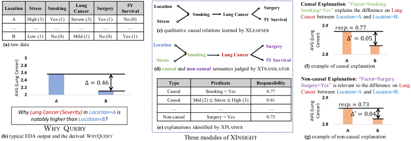
Figure 1. Illustrative example of XInsight.

According to Pearl’s general causality (judea2009causal, 40), causal knowledge is typically represented by causal graphs. Each node in a causal graph represents a random variable in data, and each directed edge between parent and child nodes denotes a cause-effect relation. Causal knowledge primarily conveys qualitative explanations (scheines1991qualitative, 50), such as smoking causes lung cancer. To further enable quantitative explanations, it is necessary to quantify the contribution of each input to the output. This way, we quantify smoking’s contribution to lung cancer and compare it with other factors. Halpern’s actual causality (halpern2005causes, 19, 18), and essentially its adaptation, DB Causality [30], provide an elegant formulation of this concept.

This paper proposes XInsight as a unified, causality-based XDA framework that qualitatively and quantitatively answers Why Query raised by users. Considering the following Why Query:

Example 1.1.

The dataset in Fig. 1(a) depicts the patient information in a country. An analyst observes an interesting data fact: “the average severity of lung cancer of patients in location A is much higher than in location B” and then raises a Why Query (Fig. 1(b)).

for which Fig. 1(f) and (g) illustrate two explanations provided by XInsight. Each explanation is flagged as either a “causal” or “non-causal” explanation, and is composed of both qualitative and quantitative sub-explanations.

Example 1.2.

An explanation (Fig. 1(f)) deems “Smoking” to be a qualitative causal factor of lung cancer severity and highlights “Smoking=Yes” and its responsibility as a quantitative sub-explanation.

XInsight includes three modules, XLearner, XTranslator, and XPlainer to gradually form explanations. XLearner first automatically discovers a causal graph $\mathcal{G}$ from data (Fig. 1(c)). Then, given a Why Query (Fig. 1(b)) with the target (i.e., the measure “Lung Cancer”) and the context (i.e., the breakdown dimension “Location”), XTranslator enumerates each remaining variable on $\mathcal{G}$ and decides if it is causal or non-causal to the target under the context. Fig. 1(d) shows causal variables (i.e., those that can potentially provide causal explanations) in green and non-causal variables (i.e., those that can potentially provide non-causal explanations) in purple. Last, XPlainer quantifies how well each variable answers Why Query by searching possible predicates on the variables that are the most responsible, as shown in Fig. 1(e). Despite the promising capability of XInsight, concretizing each module is challenging. We brief the challenges and our solutions in the following.

XLearner. Most real-world datasets are collected irrespective of causal sufficiency (peters2017elements, 43). In other words, not all causally relevant variables are available in the dataset. Furthermore, real-world datasets often contain deterministic relations in the form of Functional Dependency (FD), especially when they have materialized from relational databases. These FDs may violate the faithfulness assumption (ding2020reliable, 12), which is crucial for many causal discovery algorithms. To address these challenges, we establish a theory to propose an FD-induced graph $\mathcal{G}_{\texttt{FD}}$. XLearner uses $\mathcal{G}_{\texttt{FD}}$ to select a subset of variables for standard causal discovery where the selected variables do not trigger faithfulness violations induced by FDs. It adopts FCI (zhang2008completeness, 57) to address causal insufficiency and synergistically combine the result of FCI with the causal relations entailed by $\mathcal{G}_{\texttt{FD}}$.

XTranslator. The translation from causal primitives (the structural relations in the causal graph) into XDA semantics (e.g., whether a variable provides causal explanations) is under-explored. Given a Why Query (with a target and a context), it is unclear how to determine if a variable $X$ can explain the target given the context, and, moreover, if $X$ provides causal or non-causal explanations. XTranslator characterizes various causal primitives (e.g., m-separation, ancestor/descendant relations) from a causal graph and provides a taxonomy to translate them into XDA semantics.

XPlainer. DB causality is primarily designed for data provenance, which usually provides tuples as explanations. Contrarily, we note that predicate-level explanations shall be more desirable for XDA scenarios. Moreover, computing the responsibility of explanations with DB causality is NP-complete in general (meliou2010complexity, 33). XPlainer adapts DB causality to XDA by using predicate-level explanations with the conciseness consideration and also significantly reduces the computing cost with theoretical guarantees. In summary, we make the following contributions:

• We propose XInsight, a unified and causality-based framework for XDA. XInsight features adequate (by distinguishing causal from non-causal) and comprehensive (with qualitative and quantitative) explanations.

• XInsight consists of three modules, XLearner, XTranslator and XPlainer, each of which is meticulously designed to address technical challenges and deliver efficient analysis. XLearner learns the causal graph from causally insufficient data in the presence of FD-induced faithfulness violations, XTranslator translates causal primitives into XDA semantics, and XPlainer efficiently provides quantitative explanations via an adaptation of DB causality to meet the needs of XDA scenarios.

• Empirically, we conduct thorough experiments on public data, production data, and synthetic data via quantitative experiments and human evaluations. The results are very encouraging.

Open Source and Real-world Adoption. We release our code at (code, 36). XPlainer has been integrated into Microsoft Power BI to explain increase/decrease in data (pbi, 37).

2. Preliminary

2.1. Data Model and Query

Multi-Dimensional Data. Let $D\coloneqq\{X_{1},\cdots,X_{n}\}$ represents multi-dimensional data comprising $n$ attributes. In XInsight, we assume that records of $D$ are drawn independently from an identical distribution without selection biases (i.e, i.i.d. assumption) such that each attribute is a (random) variable. Here, selection bias is a preferential selection of units in data analysis (bareinboim2012controlling, 5). A variable is either categorical or numerical. In accordance with previous works (ma2021metainsight, 28, 11), we denote a categorical variable as dimension and a numerical variable as measure. Multi-dimensional data is commonly represented as a spreadsheet in our context. For relational data, we anticipate taking a materialized provenance table (li2021putting, 24) as input.

Aggregation and Discretization on Measure. Given a measure $M$, users may perform aggregation operations (such as SUM and AVG in SQL) over a set of realizations of $M$. In some cases, measures are processed in the form of a dimension (e.g., use measures for explanations), which necessitates discretization. It transforms numerical values into several discrete bins that form a categorical variable.

Filter. In this paper, filter is the basic unit of data operations. Given a multi-dimensional data $D$ and a dimension $X$, a filter $p_{i}=\{X=x_{i}\}$ (e.g., “Smoking=Yes”) implies an equality assertion to $X$ such that the value of $X$ shall equal $x_{i}$.

Predicate. The disjunction of filters applied on the same dimension is a predicate. Given the dimension $X$, the predicate $P(x_{1},\cdots,x_{k})$ is a set containment assertion $\{X=x_{1}\lor\cdots\lor X=x_{k}\}\equiv\{p_{1},\cdots,p_{k}\}$. On a discretized measure, a predicate is an assertion on ranges. A filter is a special case of a predicate. For clarity, we represent a general predicate with a capital $P$ and a filter with a lower-case $p$.

Subspace. A subspace is a conjunction of filters on disjointed dimensions. Given multi-dimensional data $D$, a subspace corresponds to a subset of rows satisfying the conditions of all filters. If two subspaces only differ in one filter, they are regarded as siblings. The term Context refers to the variables of two sibling subspaces, where the background variables are the variables with the shared filters and the foreground variables are the variables with the different filters. In the following example, we provide a simple instantiation.

Example 2.1.

Consider the preceding dataset in Fig. 1(a). $s=\{\text{Location}=\text{A}\land\text{Lung Cancer}=\text{Severe}\}$ represents the subspace denoting all patients in “Location=A” with severe lung cancer. All patients in “Location=A” with severe lung cancer and all patients in “Location=B” with severe lung cancer form a pair of sibling subspaces. Here, “Location” is the foreground variable and “Lung Cancer” is the background variable.

Selection. We use the following notation to represent the selection procedure over multi-dimensional data $D$. The subset of data after the selection operation is defined as $D_{p_{i}}$, $D_{P}$, or $D_{s}$, where $p_{i}$ is a filter, $P$ is a predicate, and $s$ is a subspace. We define $D-D^{\prime}$ as the rows remaining in $D$ after removing those from $D^{\prime}$.

Why Query and Explanation. As illustrated in Fig. 1(b), the user would issue a Why Query to XInsight for explanation. We formally define Why Query as follows.

Definition 2.0 (Why Query).

Given a multi-dimensional data $D$, a user launches aggregate query $agg()$ on a target measure $M$ under two sibling subspaces $s_{1},s_{2}$. Why Query is defined as $\Delta_{s_{1},s_{2},M,agg}(D)=agg_{M}(D_{s_{1}})-agg_{M}(D_{s_{2}})$. For brevity, we use $\Delta(D)$ as the shorthand of $\Delta_{s_{1},s_{2},M,agg}(D)$. W.l.o.g., we assume $\Delta$ is always non-negative.

Example 2.3.

As shown in Fig. 1(b), we concretize the Why Query $\Delta$ with the AVG aggregate on the target “Lung Cancer” over two sibling subspaces $s_{1}=\{\text{Location}=\text{A}\},s_{2}=\{\text{Location}=\text{B}\}$, denoting the difference in average lung cancer severity in “A” and “B”.

Indeed, explaining the difference between two aggregate queries is one prevalent data analysis task. Identifying the cause in data difference constitutes the basis of many data explanation applications, such as outlier explanation and data debugging (glavic2021trends, 17). In accordance with prior works (wu2013scorpion, 54, 1, 17), we concretize the problem of XDA by concentrating on the explanation of data difference. The following form is used to provide explanations in response to Why Query.

Definition 2.0 (Explanation).

Given a Why Query, an explanation is represented by the following triplet

(1) $$\textit{explanation}\coloneqq\left\langle\textit{type},\textit{predicate},\textit{responsibility}\right\rangle\vspace{-5pt}$$

where $\textit{type}\in\{\textit{causal},\textit{non-causal}\}$ denotes whether the explanation is causal or non-causal, the predicate is the content of the explanation, and responsibility, and a score ranging from 0 to 1 quantifies the extent to which the explanation explains the given Why Query.

Example 2.5.

Fig. 1(e) lists several explanations to the Why Query. Fig. 1(f)-(g) visualize two of them. Fig. 1(f), as a causal explanation, depicts that “Smoking=Yes” causes the lung cancer severity difference in Location A and B with a responsibility of $0.77$.

Single- vs. Multi-Dimensional Explanation. For conciseness and clarity, we anticipate that each explanation reflects one aspect contributing to the outcome when explaining the Why Query. We recommend adopting a single-dimensional explanation in XInsight due to its unambiguous causal semantics, although it is feasible to extend an explanation as multi-dimensional using the Cartesian product. The joint causal semantics of several variables, however, could be obscure. Furthermore, multiple single-dimensional explanations (e.g., Fig. 1(e)) suffice to represent a multi-dimensional case.

Functional Dependency (FD). Functional dependency relations are common in multi-dimensional data. In a relational database, among the attributes, there may exist primary keys and foreign keys. Therefore, after materialization, the resulting multi-dimensional data may have functional dependencies. A functional dependency between $X$ and $Y$ is represented by $X\xrightarrow{\texttt{FD}}Y$. FD, as a deterministic relation among two variables, deems a form of reliable knowledge. This research focuses on one-to-one and one-to-many FDs. We present a simple exemplary dataset that contains FDs.

Example 2.6.

Let CityInfo be a dataset with three attributes (i.e., City, State, Country). It has three FDs, namely, $\text{City}\xrightarrow{\texttt{FD}}\text{State}$, $\text{State}\xrightarrow{\texttt{FD}}\text{Country}$, and $\text{City}\xrightarrow{\texttt{FD}}\text{Country}$.

FD-Induced Graph. Given a multi-dimensional data $D$ and its functional dependencies, the FD-induced Graph $\mathcal{G}_{\texttt{FD}}\coloneqq(V,E)$, where $V\coloneqq\{X_{i}\mid\forall X_{i}\in D\}$ and $E\coloneqq\{(X_{i},X_{j})\mid\text{if }X_{i}\xrightarrow{\texttt{FD}}X_{j}\}$. We assume $\mathcal{G}_{\texttt{FD}}$ to be acyclic. Cycles in $\mathcal{G}_{\texttt{FD}}$ imply redundant attributes; in such cases, we retain only one of them to ensure acyclicity.

2.2. Causal Discovery with Latent Variables

This section presents terminology essential to causal discovery with latent variables, such as the representation of causal graphs under causal insufficiency and typical assumptions in causal discovery.

Causal Sufficiency. Causal discovery aims to learn the causal relations from the observational data. Most causal discovery algorithms assume a sufficient observation of the underlying data generating process (spirtes2000causation, 51). Formally, a set of variables $\bm{X}$ is said to be causally sufficient if there is no hidden variable $Z\notin\bm{X}$ that is causing more than one variable in $\bm{X}$. In other words, it assumes that latent confounders — the shared causes among two or multiple variables — do not exist. However, the process used to acquire real-world data does not provide such guarantees, thereby often yielding causally insufficient observations. Hence, the causal discovery procedure is compromised by the spurious association between two variables sharing a latent confounder. We present an example below.

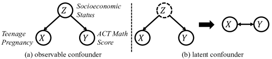
Figure 2. Examples of observable and latent confounders.

Example 2.7.

Consider the hypothetical causal graph in Fig. 2(a) where the socioeconomic status ($Z$) simultaneously causes teenage pregnancy ($X$) and their ACT math scores ($Y$). The socioeconomic status, however, does not appear in the dataset. This absence yields an insufficient observation (the left-side causal graph in Fig. 2(b)), which further results in a spurious association (pearl2009causality, 41) of teenage pregnancy and ACT math scores (the bidirected edge in Fig. 2(b)).

Hence, popular directed acyclic graphs are not expressive enough to represent these subtle relations. This necessitates the Maximum Ancestral Graph (spirtes2000causation, 51), which is introduced shortly.

Notation and Terminology. Recall that we assume the dataset is i.i.d. with potential latent confounders and does not contain selection bias. Maximal Ancestral Graph (MAG) forms the standard representation of causal graphs in this setting. We now introduce important concepts of graphical models and properties of MAG.

A directed mixed graph $\mathcal{G}$ is a graphical model that contains nodes $\bm{X}$ and two types of edges, including directed ($\to$) and bidirected ($\leftrightarrow$). There is at most one edge between any two nodes. For each directed edge $X\to Y$, $X$ is a parent of $Y$ and $Y$ is a child of $X$. $X$ and $Y$ are adjacent if there is an edge (either directed or bidirected) between them. A path $\mathcal{P}$ is a sequence of distinct nodes $(X_{1},\ldots,X_{k})$ where $X_{i}$ and $X_{i+1}$ are adjacent in $\mathcal{G}$ for all $1\leq i<k$. A path $\mathcal{P}=(X_{1},\ldots,X_{k})$ is directed if $X_{i}$ is a parent of $X_{i+1}$ for all $1\leq i<k$. $X$ is an ancestor of $Y$ if there exists a directed path from $X$ to $Y$ and $Y$ is a descendant of $X$ accordingly. Given a path $(X_{1},\ldots,X_{k})$, a non-endpoint node $X_{i}$ is a collider if there are arrowheads pointing to $X_{i}$ from both $X_{i-1}$ and $X_{i+1}$. Below, we list all possible cases of a collider.

Example 2.8.

Given $(X_{i-1},X_{i},X_{i+1})$, $X_{i}$ is a collider if and only if a) $X_{i-1}\to X_{i}\leftarrow X_{i+1}$, or b) $X_{i-1}\leftrightarrow X_{i}\leftarrow X_{i+1}$, or c) $X_{i-1}\to X_{i}\leftrightarrow X_{i+1}$, or d) $X_{i-1}\leftrightarrow X_{i}\leftrightarrow X_{i+1}$. In Fig. 1(c), Smoking is a collider of Location and Stress since “Location ${\circ\hskip 0.85358pt\!\!\!\rightarrow}$ Smoking ${\leftarrow\hskip 0.85358pt\!\!\!\circ}$ Stress”, where $\circ$ represents an undetermined edge endpoint.

A path $(X,W_{1},\cdots,W_{k},Y)$ is said to be blocked by $Z\subseteq\bm{X}\setminus\{X,Y\}$ if there exists a node $W_{i}\in\{W_{1},\cdots,W_{k}\}$ such that a) $W_{i}$ is not a collider but a member of $Z$, or b) $W_{i}$ is a collider but not an ancestor of any nodes of $Z$. We now introduce m-separation and MAG.

Definition 2.0 (m-separation (zhang2008completeness, 57)).

$X,Y$ are m-separated by $Z$ (denoted by $X{\Perp_{\mathcal{G}}}Y\mid Z$) if all paths between $X,Y$ are blocked by $Z$.

Example 2.10.

Consider the causal graph in Fig. 1(c) where “Smoking” blocks the only path between “Location” and “Lung Cancer”. Hence, “Smoking” m-separates “Location” and “Lung Cancer” (denoted by $\text{Lung Cancer}{\Perp_{\mathcal{G}}}\text{Location}\mid\text{Smoking}$).

Definition 2.0 (Maximal Ancestral Graph (zhang2008completeness, 57)).

A directed mixed graph is called a MAG if a) it contains no directed cycles or almost directed cycles and b) for each pair of non-adjacent nodes, there exists a set of nodes that m-separates them. A directed cycle refers to the case where $X\to Y\to\cdots\to X$ and an almost directed cycle refers to the case where $X\to Y\to\cdots\to Z\leftrightarrow X$.

Then, the Global Markov Property (GMP) is developed to provide a probabilistic interpretation of m-separation.

Definition 2.0 (Global Markov Property (spirtes2000causation, 51)).

(2) $$X{\Perp_{\mathcal{G}}}Y\mid Z\Rightarrow X\Perp Y\mid Z\vspace{-5pt}$$

As aforementioned, m-separation indicates that all paths between $X$ and $Y$ are “blocked” by $Z$. Hence, it is intuitive that, if $X$ and $Y$ are m-separated, their statistical correlation is also “blocked” by $Z$. The term conditional independence (i.e., $X\Perp Y\mid Z$) depicts this absence of statistical correlation. Statistically, $X\Perp Y\mid Z$ implies that $P(X,Y\mid Z)=P(X\mid Z)P(Y\mid Z)$, which can be empirically examined using statistical hypothesis tests (e.g., $\chi^{2}$ tests).

Example 2.13.

Consider the dataset in Fig. 1(a). According to GMP, the m-separation in Ex. 2.10 implies that, for the dataset in Fig. 1(a), “Location” and “Lung Cancer” are conditionally independent given “Smoking,” in a statistical sense.

With GMP, we can deduce statistical conditional independence in data from m-separations. Note that only data is available when performing causal discovery. Hence, we need to invert GMP and establish a connection from data distribution to the graphical structure. Faithfulness assumption establishes such connection.

Definition 2.0 (Faithfulness (spirtes2000causation, 51)).

(3) $$X\Perp Y\mid Z\Rightarrow X{\Perp_{\mathcal{G}}}Y\mid Z$$

According to faithfulness, if we observe that two variables are conditionally independent by a set of variables in data, then they are m-separated by the same set of variables on the causal graph. Faithfulness and GMP together establish the equivalence between conditional independence and m-separation and they form the key to causal discovery. In addition, we define skeleton as follows.

Definition 2.0 (Skeleton).

The skeleton $\mathcal{S}$ of a MAG $\mathcal{G}$ is the undirected graph obtained by removing all arrowheads from $\mathcal{G}$.

Constraint-based Causal Discovery. Constraint-based approaches are the standard solution to causal discovery. With the faithfulness assumption, these methods exploit the conditional independence derived from data and gradually establish a MAG $\mathcal{G}$. $\mathcal{G}$ is consistent with all m-separations entailed by conditional independence. However, there may exist multiple MAGs that are equally consistent with the m-separations and not distinguishable, which is called Markov equivalence class, denoted by $[\mathcal{G}]$. It is worth noting that these feasible MAGs share the same skeleton while differing in direction on certain edges. These MAGs are therefore summarized into a compact representation called Partial Ancestral Graph (PAG) with some undetermined edge endpoints.

Table 1. Four types of edges in PAG. Circle represents undetermined edge endpoint (can be either an arrowhead or tail).

Edge	Causal Semantics
$X\rightarrow Y$	$X$ is a cause of $Y$.
$X\leftrightarrow Y$	neither $X$ nor $Y$ is a cause of each other but they share a latent common cause.
$X{\circ\hskip 0.85358pt\!\!\!\rightarrow}Y$	1) $X$ is a cause of $Y$; or 2) neither $X$ nor $Y$ is a cause of each other but they share a latent common cause.
$X{\circ\hskip 1.13809pt\!\!\!-\hskip 1.13809pt\!\!\!\circ}Y$	1) $X$ may be a cause of $Y$; or 2) $Y$ may be a cause of $X$; or 3) neither $X$ nor $Y$ is a cause of each other but
	they share a latent common cause.

Definition 2.0 (Partial Ancestral Graph (zhang2008completeness, 57)).

Let $[\mathcal{G}]$ be a Markov equivalence class of a MAG $\mathcal{G}$. A PAG for $[\mathcal{G}]$ is a graph $\mathcal{P}$ with three possible edge endpoints (namely, tail, circle and arrowhead; and hence four kinds of edges: $\to,\leftrightarrow,{\circ\hskip 0.85358pt\!\!\!\rightarrow},{\circ\hskip 1.13809pt\!\!\!-\hskip 1.13809pt\!\!\!\circ}$) such that 1) $\mathcal{P}$ shares the same adjacencies with $\mathcal{G}$ (and any member of $[\mathcal{G}]$), and 2) every non-circle edge endpoint indicates an invariant edge endpoint in $[\mathcal{G}]$.

The second condition in Def. 2.16 implies that an edge associates a tail “$-$” or arrowhead “$\to$” endpoint, if and only if it is invariant in all $\mathcal{G}\in[\mathcal{G}]$. Table 1 lists the semantics of edges.

Example 2.17.

$\text{Location}~{}{\circ\hskip 0.85358pt\!\!\!\rightarrow}~{}\text{Smoking}$ in Fig. 1 (c) implies that “Location” is a cause of “Smoking” or they share a latent confounder.

We clarify that the FCI algorithm (spirtes2000causation, 51), as a typical constraint-based approach, consists of two phases. The skeleton of $[\mathcal{G}]$ is first learned by assuming faithfulness (i.e., the FCI-SL phase of the FCI algorithm). Then, the undirected edges are subsequently oriented according to a set of orientation rules (i.e., the FCI-Orient phase of the FCI algorithm). Finally, the PAG is returned; see full details of the FCI algorithm in Supplementary Material. However, soon we will show that the faithfulness assumption can be violated by FD relations. In this paper, we focus on establishing a theory and proposing a solution to tackle this unique challenge that arises in data analysis scenarios. That is, our XLearner calibrates the FCI algorithm to correctly handling FDs (see details in Sec. 3.1).

3. XInsight

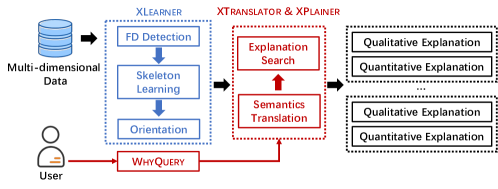
Figure 3. Workflow of XInsight. Offline phase is marked in blue and online phase is marked in red.

XInsight delivers a unified framework for XDA with three modules. The workflow of XInsight is shown in Fig. 3. First, given a multi-dimensional data $D$, XLearner pre-learns a causal graph $\mathcal{G}$ from data in the offline phase (blue-annotated in Fig. 3). Then, in the online phase (red-annotated in Fig. 3), upon receiving a Why Query, XTranslator identifies variables that have the potential to give either causal or non-causal explanations based on the causal primitives in $\mathcal{G}$. Finally, XPlainer examines each identified variable with potential and decides the optimal explanation for the given Why Query. After applying XPlainer to all variables with potential, XInsight yields a set of explanations (with qualitative sub-explanations and quantitative sub-explanations). By decoupling XInsight into an offline phase and an online phase, heavy-weight computations are performed beforehand, and only light-weight computations are needed in the online phase, allowing for a rapid response to a user’s query. In the following, we elaborate on the design of each module. Due to page limits, we present proofs and theoretical discussion in the Supplementary Material.

3.1. XLearner

XLearner aims to learn a causal graph $\mathcal{G}$ from multi-dimensional data $D$ in the presence of latent confounders. The primary obstacle is that learning the skeleton of $\mathcal{G}$ requires the faithfulness assumption (see Sec. 2.2), which may be violated by FDs in $D$. Below, we show how contradictory causal structures can be induced when being agnostic to FDs.

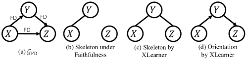
Figure 4. Illustration of FD-induced faithfulness violation.

Example 3.1.

We first consider the CityInfo dataset described in Ex. 2.6 and the corresponding FD-induced graph in Fig. 4(a), where $X$ denotes city, $Y$ denotes state, and $Z$ denotes country. By definition of conditional independence (i.e., $X\Perp Y\mid Z\iff P(X,Y\mid Z)=P(X\mid Z)P(Y\mid Z)$), we have $Y\Perp Z\mid X$ and $X\Perp Z\mid Y$. The definition of faithfulness implies $Y{\Perp_{\mathcal{G}}}Z\mid X$ and $X{\Perp_{\mathcal{G}}}Z\mid Y$, given $Y\Perp Z\mid X$ and $X\Perp Z\mid Y$. $Z$ is non-adjacent to both $X$ and $Y$ according to the m-separation definition (see the induced graph in Fig. 4(b)). Consequently, $Z$ is an isolated node in Fig. 4(b). We have $Y{\Perp_{\mathcal{G}}}Z$ and GMP further implies that $Y\Perp Z$, which contradicts $Y\not\Perp Z$ entailed by $Y\xrightarrow{\texttt{FD}}Z$. Indeed, the skeleton is not consistent with any MAGs that are on the top of it.

Table 2. Comparing different causal discovery algorithms. ✓ denotes “support” whereas ✗ denotes “no support”.

Alg.	Orientation	FD-induced Faithfulness Violation	Causal Insufficiency
PC (spirtes2000causation, 51)	✓	✗	✗
FCI (zhang2008completeness, 57)	✓	✗	✓
REAL (ding2020reliable, 12)	✗	✓	✗
XLearner	✓	✓	✓

As aforementioned in Sec. 2, the violations of causal sufficiency and faithfulness (induced by FDs) are common in the data analysis scenarios. However, they are addressed separately in the literature, as reviewed in Table 2. XLearner focuses on addressing both challenges simultaneously. Fig. 4(c)-(d) show the skeleton and orientation by XLearner, which are compliant with intuition.

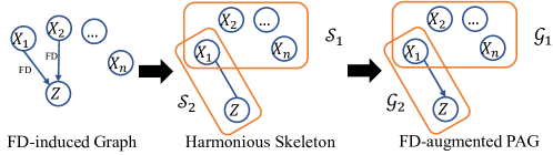
Figure 5. Running example of XLearner.

Overall, XLearner tackles the problem in three stages. We outline the workflow of XLearner in Alg. 1 and present an example. Then, we elaborate on the design of XLearner.

Example 3.2.

Consider the FD-induced graph $\mathcal{G}_{\texttt{FD}}$ shown in Fig. 5. In the first stage, XLearner uses $\mathcal{G}_{\texttt{FD}}$ to identify variables (e.g., $X_{1}$ and $Z$ in Fig. 5) that may trigger faithfulness violations. Then, the skeleton $\mathcal{S}_{2}$ is built upon a harmonious assumption instead of faithfulness over $X_{1}$ and $Z$. In the second stage, the FCI algorithm (skeleton learning and orientation) is only conducted over variables that comply with the faithfulness assumption. Hence, the skeleton $\mathcal{S}_{1}$ and the PAG $\mathcal{G}_{1}$ are identified accordingly. In the third stage, we orient $\mathcal{S}_{2}$ to generate an FD-augmented PAG $\mathcal{G}_{2}$. By concatenating $\mathcal{G}_{1}$ and $\mathcal{G}_{2}$, the resultant (FD-augmented) PAG $\mathcal{G}$ is obtained.

Input: Multi-dimensional Data $D$, FD-induced graph $\mathcal{G}_{\texttt{FD}}$

Output: FD-augmented PAG $G$

1 // stage 1: detect and preclude $\bm{X}_{\texttt{FD}}$ (Sec. 3.1.1)

2 $\mathcal{S}_{2}\leftarrow(V,\emptyset)$;

3 Topologically sorting nodes in $\mathcal{G}_{\texttt{FD}}$ and record depth as $d(X_{i})$;

4 while $\mathcal{G}_{\texttt{FD}}$ has non-root nodes do

5       $X\leftarrow\operatorname*{argmax}_{X\in\mathcal{G}_{\texttt{FD}}.V}d(X)$;

6       $Y\leftarrow\operatorname*{argmin}_{Y\in Pa(\mathcal{G}_{\texttt{FD}},X)}|Y|$;

7       add edge $(X,Y)$ in $\mathcal{S}_{2}$;

8       remove $X$ and all connected edges from $\mathcal{G}_{\texttt{FD}}$;

9      

10 end while

11// stage 2: standard PAG learning

12 $\mathcal{S}_{1}\leftarrow\texttt{FCI-SL}(D,\mathcal{G}_{\texttt{FD}}.V)$;

13 $\mathcal{G}_{1}\leftarrow\texttt{FCI-Orient}(S_{1})$;

14 // stage 3: orient $\mathcal{S}_{1}$ and generate $\mathcal{G}$ (Sec. 3.1.2)

15 foreach $(X\xrightarrow{\texttt{FD}}Y)\in\mathcal{G}_{\texttt{FD}}.E$ do

16       if $X,Y$ is adjacent in $\mathcal{S}$ then  orient $X\rightarrow Y$ on $\mathcal{G}^{2}$ ;

17      

18 end foreach

19generate $\mathcal{G}$ concatenating $\mathcal{G}^{1}$ and $\mathcal{G}^{2}$;

20 return $\mathcal{G}$;

Algorithm 1 XLearner procedure.

Comparison with FCI. Comparing with the FCI algorithm (spirtes2000causation, 51, 57), XLearner for the first time reconciles functional dependency (FD) and the faithfulness assumption for causally insufficient data within the harmonious skeleton framework. In that sense, it can learn causal graphs from real-world data adequately. As validated in Sec. 4.3, XLearner learns more accurate causal graphs than the FCI algorithm. Second, it uses FDs to provide a more complete orientation to the underlying causal graph. Hence, compared to the FCI algorithm, it leverages the knowledge from FDs to enforce a more precise causal graph with less undetermined edges. In sum, we deem that XLearner enhances the FCI algorithm from the theoretical perspective, and also addresses obstacles in the real-life adoption of the FCI algorithm.

3.1.1. Skeleton Learning with FD (lines 1–9 of Alg. 1)

Ding et al. point out that in the presence of FD relations, faithfulness assumption can be violated thus we can at most obtain a harmonious skeleton (ding2020reliable, 12). However, the original theory of harmonious skeletons is established under causal sufficiency. Here, we further generalize the harmonious skeleton for causally insufficient systems:

Definition 3.0 (Harmonious Skeleton).

A skeleton $\mathcal{S}$ is said to be harmonious w.r.t. a joint probability distribution $P$ if 1) there exists a MAG $\mathcal{G}$ sharing the same adjacencies of $\mathcal{S}$, 2) $P$ satisfies GMP to $\mathcal{G}$, and 3) any subgraph of $\mathcal{S}$ does not satisfy the previous two conditions.

Def. 3.3 entails three properties of $\mathcal{S}$. First, since there exists a MAG $\mathcal{G}$ on top of the skeleton $\mathcal{S}$, there exists a set of nodes that m-separates any non-adjacent nodes. Second, if two nodes (e.g., $X,Y$) are m-separated by $Z$, then $X\Perp Y\mid Z$. These two conditions imply that $X$ and $Y$ are non-adjacent in $\mathcal{S}$, if and only if there exists a set of nodes $Z$ such that $X\Perp Y\mid Z$. The last condition implies the minimality of $\mathcal{S}$, which is commonly assumed (peters2017elements, 43). When two graphs $\mathcal{G},\mathcal{G}^{\prime}$ are equally compatible with the data, we would prefer the simpler one. We now show the construction of $\mathcal{S}$, which begins with a basic case and generalizes to arbitrary structures.

Theorem 3.4.

Let $Z$ be a sink node (i.e., all edges of $Z$ are oriented to $Z$) in $\mathcal{G}_{\texttt{FD}}$. $\mathcal{S}=\mathcal{S}_{1}\cup\mathcal{S}_{2}$ is a harmonious skeleton if 1) $S_{1}$ is a harmonious skeleton over $\bm{X}\setminus Z$ and $\mathcal{S}_{2}$ contains only one edge $X_{i}-Z$ where $X_{i}$ can be any node connected to $Z$ in $\mathcal{G}_{\texttt{FD}}$.

Example 3.5.

Fig. 5 presents an example of Thm. 3.4. Connecting the sink node $Z$ with one of its parents $X_{1}$ in the $\mathcal{G}_{\texttt{FD}}$ yields a skeleton $\mathcal{S}_{2}$. If we can learn a harmonious skeleton $\mathcal{S}_{1}$ on the remaining nodes ($X_{1},\cdots,X_{n}$), Thm. 3.4 ensures that concatenating $\mathcal{S}_{1},\mathcal{S}_{2}$ produces a harmonious skeleton over all variables.

According to Thm. 3.4, if $Z$ has more than one parent, multiple harmonious skeletons exist (note that $Z$ can connect to any one of its parents). In practice, we connect $Z$ to the parent node with the lowest cardinality. Given a FD-induced graph, we recursively apply Thm. 3.4 to identify sink nodes and derive the corresponding harmonious skeleton $\mathcal{S}_{2}$ until all FDs are properly resolved. Then, we can apply the standard skeleton learning algorithm over the remaining nodes. The procedure is shown in lines 1–9 in Alg. 1.

Theorem 3.6.

The skeleton of Alg. 1 is harmonious.

Alg. 1 first constructs an empty skeleton $\mathcal{S}$ that shares the same nodes as $\mathcal{G}_{\texttt{FD}}$ (line 2). At line 3, we topologically sort the $\mathcal{G}_{\texttt{FD}}$ nodes (note that $\mathcal{G}_{\texttt{FD}}$ is a DAG). In each iteration (lines 5–8), we pick the deepest node and apply Thm. 3.4 to connect $X$ to one of its parents (in $\mathcal{G}_{\texttt{FD}}$) $Y$ in the skeleton. We use the parent node with the lowest cardinality as $Y$ (line 6), as it usually aligns with human intuition.

Example 3.7.

Consider the CityInfo dataset in Ex. 2.6. Alg. 1 identifies the correct skeleton as $\text{City}-\text{State}-\text{Country}$ in Fig. 4(c).

For root nodes, since there are no FDs and thus the faithfulness assumption holds, we employ the standard FCI algorithm (lines 10–12) to infer the PAG $\mathcal{G}_{1}$. After $\mathcal{S}_{2}$ being oriented to $\mathcal{G}_{2}$ (see Sec. 3.1.2), we concatenate them to form $\mathcal{G}$ (line 17). Thm. 3.6 proves that the skeleton of $\mathcal{G}$ is also harmonious after the concatenation.

3.1.2. Orientation (lines 13–16 of Alg. 1)

Classical constraint-based causal discovery algorithms decide the direction of edges based on a set of orientation rules. These rules orient undirected edges on skeletons (i.e., ${\circ\hskip 1.13809pt\!\!\!-\hskip 1.13809pt\!\!\!\circ}$) based on a set of criteria, including conditional independence and some graphical structural relations (e.g., discriminating path) (zhang2008completeness, 57). These rules are applied iteratively until no more orientations can be made. However, we argue that an FD itself reflects a causal relation to a good extent, of which the reason is twofold.

ANM Perspective on FD-related Edges. We anticipate incorporating the discrete additive noise model (ANM) (peters2011causal, 42) for orienting FD-related edges. The main theory of ANM implies that if an asymmetric ANM $Y=f(X)+N_{Y}$ exists from $X$ to $Y$ and $N_{Y}$ is independent of $X$, then $X$ causes $Y$. By FD, we note that, if $X\xrightarrow{\texttt{FD}}Y$ in $\mathcal{G}_{\texttt{FD}}$, an ANM construction from X to Y naturally exist with noise term $N_{Y}=0$. On the other hand, an ANM construction from $Y$ to $X$ exists only in very rare cases, as determined by the identifiability of the discrete ANM (see Thm. 4.6 in (peters2017elements, 43)). In light of this, we hypothesize that $X\xrightarrow{\texttt{FD}}Y$ in $\mathcal{G}_{\texttt{FD}}$ implies causation of $X\to Y$.

FCI Perspective on FD-related Edges. The rules in FCI may be unreliable due to the faithfulness violations by FDs. However, an FD itself is generally more reliable, which describes deterministic relations. More importantly, the directions from the FDs are compatible with the result of the FCI on the variables excluding FD-related variables. That is, incorporating ANM would not violate GMP.

We implement the above hypothesis in our orientation algorithm (lines 13–16 in Alg. 1). We examine, for each FD relation that is also adjacent in $\mathcal{S}_{2}$, whether the edge is oriented as $\rightarrow$ (lines 13–15). We note that, by incorporating ANM, the augmented graph is more informative and represents an overcomplete graph w.r.t. the ground-truth MAG’s Markov equivalence class, exhibiting greater precision than causal graphs learned only by rules.

3.2. XTranslator

A causal graph does not directly reveal if a variable adequately explains a Why Query, nor does it directly reflect if the variable features a causal or non-causal explanation. Bridging this gap requires a translation from causal primitives to XDA semantics. To illustrate, we start with a Why Query under AVG. We then show how to generalize the main result into SUM and other aggregates.

Principle of Explainability. Given a Why Query $\Delta$ where $agg=\texttt{AVG}$, a variable $X$ is said to have No Explainability if $X\Perp M\mid F\cup\bm{B}$, where $M$ is the target measure, $F$ is the foreground variable, and $\bm{B}$ are background variable(s). In the subsequent discussion, we omit $\bm{B}$ for the ease of presentation without loss of generality.

A Why Query in XDA requires us to observe the difference between aggregates on $M$ within two subspaces. The conditional independence of $X\Perp M\mid F$ implies that $\mathbb{E}(M\mid F,X)=\mathbb{E}(M\mid F)$. Hence, $\Delta(D)=\Delta(D_{X=x})$ in the large sample limit for all feasible filters in $X$. If $X$ is conditionally independent of $M$ given $F$, $X$ is simply impossible to offer explanations to the Why Query. Thus, this principle imposes a restriction on possible variables that have the potential to provide explanations. In particular, we derive the following restriction.

Proposition 3.0.

If $X$ has explainability, $M,X$ are not m-separated by $F$ in the causal graph $G$.

Proposition 3.8 illustrates the chance of pruning variables for which it is impossible to provide explanations. Table 3 further depicts the translation from causal primitives to XDA semantics. In XTranslator, a variable $X$ is first confirmed to have explainability if $X,M$ are not m-separated by $F$ in $G$ (1st row in Table 3). In addition, XTranslator also categorizes whether $X$ is causal or non-causal according to Table 3. Overall, $X$ provides a causal explanation if it is explainable and a cause (➀ and ➁ in Table 3) or a possible cause (➂ and ➃ rows in Table 3) of $M$. We show how the causal graph identified by XLearner is translated.

Example 3.9.

Given the dataset in Fig. 1(a), XLearner identifies the corresponding causal graph in Fig. 1(c). With the Why Query in Fig. 1(b), XTranslator translates the causal graph into the XDA semantics in Fig. 1(d). “Smoking” and “Stress Level” can be used to causally explain “Lung Cancer”. And, other variables (e.g., “Surgery”) are deemed non-causal explanations (last row in Table 3).

Table 3. Translating causal primitives to XDA semantics.

Rule	Path	Causal Primitive	XDA Semantics
➀	$X\rightarrow F\rightarrow M,\cdots$	m-separated	no explainability
➁	$X\rightarrow M$	parent	causal explanation
➂	$X\rightarrow\cdots\rightarrow M$	ancestor	causal explanation
➃	$X{\circ\hskip 0.85358pt\!\!\!\rightarrow}M$	almost parent	causal explanation
➄	$X{\circ\hskip 0.85358pt\!\!\!\rightarrow}\cdots{\circ\hskip 0.85358pt\!\!\!\rightarrow}M$	almost ancestor	causal explanation
➅	others	N/A	non-causal explanation

Extension to SUM. The above formulation over explainability is established on AVG aggregates. In the following, we discuss the implications of our formulation on SUM aggregates. If $X$ has no explainability, $X\Perp M\mid F$. When we enforce $X=x$, $\Delta(D_{X=x})$ can merely be affected by the number of rows where $X=x$ in two sibling subspaces (namely a COUNT-based explanation) instead of a causal relation between $X$ and $M$ (see detailed formulation in Supplementary Material). This may be valid for explanations; nevertheless, it is typically inconsistent with the common intuition of data analysis and may not align user expectations regarding explanations (i.e., a variable explains the target). Such COUNT-based explanation is unconventional and is thus less of a concern.

Semantics Consistency. Following the above discussion, we clarify that a variable may play different roles in various aggregates. However, in our current design, XTranslator focuses primarily on variables with strong connections to $M$, which are more likely to provide desirable explanations. Therefore, the semantics of a variable are consistent across different aggregates. As clarified in Principle of Explainability above, it is appropriate for pruning uninformative variables from general aggregates, and we do not observe notable issues in practice. We leave designing more comprehensive translation rules for future research.

3.3. XPlainer

XLearner and XTranslator together provide a coarse-grained, variable-level qualitative explanation to a Why Query. For instance, “Smoking” is a causal explanation for the differences in severity of “Lung Cancer” in Locations A and B. To go one step further, XPlainer provides predicate-level quantitative explanations to answer Why Query (e.g., “Smoking=Yes” explains the difference with the responsibility of $0.77$ in Fig. 1(f)). XPlainer is on the basis of a well-establish framework, DB causality (meliou2010causality, 32) (an extension of actual causality). To ease reading, below we first provide a recap of the notations defined in Sec. 2.1. We then rewrite the formulation of DB causality in the context of XInsight in Sec. 3.3.1.

Recap of Notations. We refer to a dataset as $D$, a filter as a lowercase $p$, and a set of filters as an uppercase $P$. The subset of $D$ satisfying $p$ (or $P$) is represented by $D_{p}$ (or $D_{P}$, respectively). We use $D-D_{P}$ as the complement of $D_{P}$ in $D$. By default, $\Delta(D)$ represents the Why Query over the dataset $D$. Likewise, for arbitrary $D^{\prime}\subseteq D$, $\Delta(D^{\prime})$ represents the difference between the aggregated values of two sibling subspaces inside $D^{\prime}$.

Definition 3.0 (DB Causality (meliou2010causality, 32)).

Given a multi-dimensional data $D$ and Why Query $\Delta$, let $t$ be a tuple in $D$. $t$ is called a counterfactual cause to $\Delta$, if $\Delta(D)>\epsilon$ and $\Delta(D-\{t\})\leq\epsilon$, where $\epsilon$ is a user-defined threshold. $t$ is called an actual cause to $\Delta$, if there exists a contingency $\Gamma\subseteq D$ such that $t$ is a counterfactual cause for $D-\Gamma$ (i.e., $\Delta(D-\Gamma-\{t\})\leq\epsilon<\Delta(D-\Gamma)$).

Definition 3.0 (DB Responsibility (meliou2010causality, 32)).

Suppose $P$ is an actual cause to Why Query $\Delta$ and $\Gamma$ ranges over all valid contingencies for $P$. The responsibility of $P$ is defined as $\rho_{P}=\frac{1}{1+\min_{\Gamma}|\Gamma|}$, where $|\Gamma|$ denotes the number of tuples in the contingency.

DB causality is appealing as it offers both a normalized measure (responsibility $\in(0,1]$) and a contingency. First, when the responsibility is close to 1, it implies that the tuple is more accountable for the outcome, and when it hits 1, it is totally responsible. Second, the minimal contingency reflects the additional influential factors that, together with the tuple, are fully responsible for the outcome. The two elements form a quantitative explanation and it is useful for users to understand why the difference exists.

3.3.1. Adaption

DB causality was originally designed for data provenance. As pointed out in (meliou2014causality, 31), tuple-level explanations are usually too fine-grained for data analysis scenarios. An individual tuple usually has too little effect on the highly aggregated outcome of a large dataset. Recalling the example in Fig. 1, users would expect to know that “Smoking=Yes” causes high “Lung Cancer” severity rather than an individual patient being the cause of the high “Lung Cancer” severity. This necessitates predicate-level explanations which are easier to understand and frequently used in data analysis scenarios, and by many data explanation tools (wu2013scorpion, 54, 1). Motivated by this, we make three adaptions over DB causality (namely, W-Causality, W-Responsibility and conciseness) to support XDA. We formulate W-Causality as follows.

Definition 3.0 (W-Causality).

Given a multi-dimensional data $D$, an attribute of interest $X$ and Why Query $\Delta$, let $P\subseteq\bigcup p_{i}$ be a predicate in $D$, where $\bigcup p_{i}$ denotes the set of all possible filters on $X$. $P$ is called a counterfactual cause of $\Delta$, if $\Delta(D)>\epsilon$ and $\Delta(D-D_{P})\leq\epsilon$, where $\epsilon$ is a user-defined threshold. $P$ is deemed to be an actual cause of $\Delta$, if there is a contingency $\Gamma\subseteq\bigcup p_{i}$ such that $P$ is a counterfactual cause for $D-D_{\Gamma}$ (i.e., $\Delta(D-D_{\Gamma}-D_{P})\leq\epsilon<\Delta(D-D_{\Gamma})$), where $P\cap\Gamma=\emptyset$.

From Tuples to Predicates. Def. 3.12 transforms the tuple and contingency into two predicates. This way, explanations as well as contingencies constitute a form of intervention over the multi-dimensional data. When a contingency $\Gamma$ is applied, it indicates that, if the events related to $\Gamma$ do not happen, then the events related to $P$ are fully responsible for $\Delta$. This adaption in turn entails another adaption to the responsibility for predicate-level explanations.

Definition 3.0 (W-Responsibility).

Suppose $P$ is an actual cause to Why Query $\Delta$ and $\Gamma$ range over all valid contingencies for $P$. The responsibility of $P$ is defined as $\rho_{P}=\frac{1}{1+\min_{\Gamma}|\Gamma|_{W}}$, where $|\Gamma|_{W}$ is defined as $\max(\frac{\Delta(D-D_{P})-\Delta(D-D_{P}-D_{\Gamma})}{\Delta(D)},0)$. We let $\rho_{P}=0$ if $P$ is not an actual cause.

W-Responsibility. Instead of using the number of rows in $D_{\Gamma}$ as $|\Gamma|_{W}$, Def. 3.13 employs the truncated difference in $\Gamma$ over $\Delta$ to measure the importance of $P$. In particular, $\Delta(D-D_{P})-\Delta(D-D_{P}-D_{\Gamma})$ can be deemed as first-order finite backward difference to the function $\Delta(\cdot)$ at the point of $D-D_{P}$ and $\Gamma$ is the step size. This supplies a simple and intuitive way to understand to what extent $\Gamma$ plays an important role in reducing the difference. The large difference imposed by $\Gamma$ implies a low importance of explanation $P$ to $\Delta$; because the reduction in $\Delta$ is primarily caused by $\Gamma$ instead of $P$ itself. Therefore, the responsibility of $P$ is measured by a valid contingency $\Gamma^{*}$ (such that $\Delta(D-D_{P}-D_{\Gamma})\leq\epsilon$ and $\Delta(D-D_{\Gamma})>\epsilon$) with minimal difference on $\Delta$.

Conciseness. Using responsibility as the sole criterion is not sufficient in practical data analysis scenarios (glavic2021trends, 17). Typically, a concise explanation is preferable. Therefore, given an attribute of interest $X$, we formulate the optimal explanation of $X$ as follows.

(4) $$\operatorname*{argmax}_{P\subseteq\bigcup p_{i}}\rho_{P}-\sigma|P|$$

where $\bigcup p_{i}$ is the set of all possible filters in $X$, $|P|$ is the number of filters in $P$, and $\sigma|P|$ ($\sigma>0$) forms a conciseness regularization. In practice, we would prefer $\sigma=\nicefrac{{1}}{{m}}$ such that when all filters are picked, the score is zero.

Table 4. Different search solutions in XPlainer. FP is false positive and FN is false negative.

Solution	Complexity	Optimality
Brute-force Search	$O(2^{m})$	Optimal
Approx. Search (SUM)	$O(m\log m)$	Moderated FP; Negligible FN
Approx. Search (AVG)	$O(m^{2})$	Moderated FP&FN

3.3.2. Optimization

As pointed out in (bertossi2020score, 6, 7), computing responsibility (i.e., $\rho_{P}$) is intractable. Furthermore, solving the optimization problem in Eqn. 4 is itself difficult given $2^{m}$ search space ($m$ is the number of filters in $X$). We characterize the performance of different solutions in Table 4. First, the brute-force search is the most accurate and general method for arbitrary aggregates, despite being very slow. The explanation discovered by brute-force search is exactly the optimal explanation. In this paper, we design two approximate solutions for SUM and AVG, respectively. In particular, we first show the existence of a linearithmic approximated solution when the aggregation is SUM. This solution also has negligible false negatives, as theoretically guaranteed by a lemma on the completeness. Furthermore, we present a heuristics-based solution for AVG with quadratic complexity. Moreover, this solution should be applicable for other aggregate functions with a mild downgrade in optimality. Our evaluation (Sec. 4.4) shows that both approximations are tight and efficient in comparison to brute-force search.

Optimization for SUM. Given the additive property of SUM (i.e., $\Delta(D_{P_{1}}+D_{P_{2}})=\Delta(D_{P_{1}})+\Delta(D_{P_{2}})$), we obtain the following proposition to prune the search space.

Proposition 3.0.

If $P^{*}$ is the optimal explanation of Eqn. 4, $\forall p\in P^{*},\Delta(D_{p})>0$.

According to Proposition 3.14, the search algorithm can omit filters with a non-positive $\Delta_{i}$ (i.e., $\Delta(D_{p_{i}})$). Recall that Eqn. 4 seeks the optimal explanation. When the aggregate function is SUM, we only need to focus on filters with a reasonably high $\Delta_{i}$ without losing optimality and we define such filters as canonical filters.

Definition 3.0 (Canonical Filter and Predicate).

Without loss of generality (w.l.o.g.), given a Why Query $\Delta$ and an attribute of interest $X$, let filters $\{p_{1},\cdots,p_{m}\}$ of $X$ be ordered by $\Delta_{i}$ (i.e., $\Delta(D_{p_{i}})$) such that $\Delta_{1}\geq\cdots\geq\Delta_{m}$. We let $p_{1},\cdots,p_{j}$ be canonical filters if

(5) $$\Delta(D)-\sum_{i=1}^{j}\Delta_{i}\leq\epsilon<\Delta(D)-\sum_{i=1}^{j-1}\Delta_{i}$$

$P^{C}=\{p_{1},\cdots,p_{j}\}$ is called a canonical predicate and $\tau=\sum_{i=1}^{j}\Delta_{i}$.

With canonical filters and a corresponding canonical predicate $P^{C}$, we observe that $P^{C}$ manifests good properties. First, $P^{C}$ is the minimal counterfactual cause entailed by Eqn. 5. Our construction of canonical predicates guarantees completeness.

Proposition 3.0 (Completeness).

For SUM, given a Why Query $\Delta$, an attribute of interest $X$ and corresponding canonical predicate $P^{C}$, there exists an optimal explanation $P^{*}\subseteq P^{C}$.

The completeness proposition (Proposition 3.16) allows us to only focus on canonical filters when searching for the optimal explanation without loss of optimality. More importantly, the canonical predicate also allows us to efficiently identify actual causes and the corresponding valid contingencies.

Theorem 3.17.

For SUM, given a Why Query $\Delta$, an attribute of interest $X$ and corresponding canonical predicate $P^{C}$, $\forall P\subset P^{C}$, $P$ is an actual cause and $\overline{P}=P^{C}-P$ is a valid contingency.

The advantages of Thm. 3.17 are twofold. First, we can directly confirm valid explanations without exhaustive enumerations. Second, by the property of $\overline{P}$, we bound $P$’s responsibility ($\rho_{P}$).

Theorem 3.18.

For SUM, given a Why Query $\Delta$, an attribute of interest $X$ and corresponding canonical predicate $P^{C}$, the W-Responsibility $\rho_{P}$ of $P\subset P^{C}$ satisfies

(6) $$\frac{1}{1+\frac{\tau-\Delta(D_{P})}{\Delta(D)}}\leq\rho_{P}\leq\frac{1}{2-\frac{\Delta(D_{P})+\epsilon}{\Delta(D)}}$$

When $\Delta(D_{P})\ll\tau$ and $0<\tau\leq\Delta(D)$, $\frac{1}{1+\tau-\Delta(D_{P})}\approx\frac{1+\tau+\Delta(D_{P})}{(1+\tau)^{2}}$ and the corresponding approximation error rate $E<0.25$.

Thm. 3.18 provides a way to efficiently approximate responsibility with theoretical guarantees. In that sense, we can compute responsibility immediately and alleviate searching the minimal contingency. Let $\hat{\rho_{P}}=\frac{1+\tau+\Delta(D_{P})}{(1+\tau)^{2}}$, we can rewrite the objective function in the following form.

(7) $$\hat{\rho_{P}}-\sigma|P|=C_{1}+C_{2}\times\sum_{p_{i}\in P}(\Delta_{i}-C_{3})$$

Here, $C_{1},C_{2},C_{3}$ are constants. Then, the optimal explanation to Eqn. 7 is straightforward:

(8) $$P^{*}=\{p_{i}\mid\Delta_{i}>C_{3}\}$$

where $C_{3}=\frac{\sigma\Delta(D)}{(1+\frac{\tau}{\Delta(D)})^{2}}$. The complexity is $\mathcal{O}(m\log(m))$ (primarily in sorting filters for generating canonical predicates).

Optimization for AVG.  In terms of AVG, it is generally much more challenging due to the absence of the additive characteristics on $\Delta(D_{P})$. Therefore, the majority of the preceding propositions are not applicable. Having said that, we find the causal graph gives considerable opportunities to prune unnecessary computations.

Definition 3.0 (Homogeneous Sibling Subspace).

Given sibling subspaces $s_{1},s_{2}$ (with foreground variable $F$ and background variables $\bm{B}$), an attribute $X$ and the causal graph $G$, $s_{1},s_{2}$ are homogeneous on $X$ if $X,F$ are m-separated given $\bm{B}$ on $G$.

Proposition 3.0.

For a homogeneous AVG, given a Why Query $\Delta$, an attribute of interest $X$, a predicate $P\subseteq\bigcup p_{i}$ and a filter $p\in P$, if $\Delta(D_{p})>\Delta(D_{P})$, then $\Delta(D_{P}-D_{p})<\Delta(D_{P})$.

To practically address the search problem of AVG (Eqn. 4), we rely on greedy-based heuristics with a pruning strategy enabled by Proposition 3.20. The algorithm is outlined in Alg. 2.

Input: Why Query $\Delta$, threshold $\epsilon$, consiseness parameter $\sigma$

Output: (near) optimal explanation $P^{*}$

1 $P^{C}\leftarrow\emptyset$;

2 foreach $r=1,\cdots,\min(m,\frac{1}{\sigma})$ do

3       if $\Delta(D-D_{P^{C}})\leq\epsilon$ then  break ;

4       else

5             $\overline{P}\leftarrow\{p_{1},\cdots,p_{m}\}-P^{C}$;

6             if homogeneous then

7                   $S\leftarrow\{p_{i}\mid p_{i}\in\overline{P},\Delta_{i}>\Delta(D-D_{P^{C}})\}$;

8                   $p^{*}\leftarrow\operatorname*{argmin}_{p\in S}\Delta(D-D_{P^{C}}-D_{p})$;

9             else

10                   $p^{*}\leftarrow\operatorname*{argmin}_{p\in\overline{P}}\Delta(D-D_{P^{C}}-D_{p})$;

11             end if

12            $P^{C}\leftarrow P^{C}\cup\{p^{*}\}$;

13            

14       end if

15      

16 end foreach

17if $\Delta(D-D_{P^{C}})>\epsilon$ then return $\perp$;

18 foreach $k\in 1,\cdots,|P^{C}|$ do

19       $P_{k}\leftarrow$ top-k filters of $P^{C}$;

20       $\Gamma_{k}\leftarrow P^{C}-P_{k}$;

21       compute $\hat{\rho_{P_{k}}}$ with $\Gamma_{k}$.

22 end foreach

23return $\operatorname*{argmax}_{k}\hat{\rho_{P_{k}}}-\sigma|P_{k}|$;

Algorithm 2 XPlainer For AVG

The high-level idea behind Alg. 2 is similar to the one for SUM, which attempts to construct a canonical predicate $P^{C}$ such that $P^{C}$ forms a counterfactual cause, each subset $P\subset P^{C}$ of the canonical predicate constitutes an actual cause, and the complement set $P^{C}-P$ is a valid contingency. Unlike SUM, however, Alg. 2 does not ensure the optimality of the resulting explanation, primarily due to the incompleteness of the canonical predicate (Proposition 3.16) under AVG. Recall that $\rho_{P}$ ranges from 0 to 1 in Eqn. 4. The optimal explanation contains at most $\nicefrac{{1}}{{\sigma}}$ filters (otherwise, $\rho_{P}-\sigma|P|<0$). Hence, the canonical predicate $P^{C}$ shall contain at most $\nicefrac{{1}}{{\sigma}}$ or $m$ (i.e., the number of filters in the attribute).

Alg. 2 employs a greedy strategy to construct $P^{C}$ progressively. It starts with an empty canonical predicate (line 1) and inserts one filter in each iteration (lines 2–13). Before insertion, it checks whether $P^{C}$ is a canonical predicate (line 3) and terminates the loop if $P^{C}$ is already valid. Otherwise, it picks the remaining filters that were not chosen in earlier iterations as candidates (line 5) and inserts the filter that minimizes the difference $\Delta(D-D_{P^{C}}-D_{p_{i}})$ at the highest magnitude into $P^{C}$ (lines 6–12). When homogeneity holds and $\Delta_{i}\leq\Delta(D-D_{P^{C}})$, Alg. 2 prunes $p_{i}$ according to Proposition 3.20 (lines 7–8). Note that $\Delta_{i}$ is invariant throughout the loop; thus it only needs to be queried once. In general cases where homogeneity does not hold, Alg. 2 has to enumerate all possible filters in $\overline{P}$ (line 10). If we cannot obtain a valid canonical predicate (i.e., a counterfactual cause to $\Delta$) after the loop, Alg. 2 terminates and outputs $\perp$, indicating that it fails to find the optimal explanation within the attribute (line 15). Empirically, we do not observe such rare cases. When the canonical predicate $P^{C}$ is obtained, $\forall k=1,\cdots,|P^{C}|-1$, the top-k filters of $P_{k}\subseteq P^{C}$ is a valid actual cause and the complement set $\Gamma_{k}=P^{C}-P_{k}$ is a valid contingency. According to the termination condition in the above loop (line 3), $\Delta(D-D_{P_{k}})>\epsilon$. In addition, according to the definition of canonical predicate $\Delta(D-D_{P^{C}})=\Delta(D-D_{P_{k}}-D_{\Gamma_{k}})\leq\epsilon$, $\Gamma_{k}$ is a valid contingency to $P_{k}$. Therefore, we compute the approximated responsibility $\hat{\rho_{P_{k}}}$ by using its lower bound deduced by $\Gamma_{k}$ (line 19). After enumerating each $k$, Alg. 2 returns $P_{k}$ such that $\hat{\rho_{P_{k}}}-\sigma|P_{k}|$ is maximized (line 21). In summary, the first loop (lines 2–14) is of quadratic complexity regardless of homogeneity and the second loop is linear (lines 16–20). The total complexity is $\mathcal{O}(m^{2})$.

4. Evaluation

In this section, we evaluate XInsight to answer the following three research questions (RQs):

1. RQ1: End-To-End Performance. How can XInsight facilitate end users in explainable data analysis?

2. RQ2: XLearner Evaluation. Does XLearner effectively recover causal relations from observational data?

3. RQ3: XPlainer Evaluation. Does XPlainer accurately and efficiently yield explanations?

4.1. Datasets & User Study Setup

To the best of our knowledge, there is no real-world benchmark with manually labeled query/explanation pairs. To deliver a scientific evaluation, we conduct experiments on ① public datasets collected from previous works, ② real-world data collected from a production environment for user study and human evaluation, and ③ synthetic data with ground-truth explanations. The detailed steps for generating synthetic datasets are given in the Supplementary Material. We make necessary preprocessing before feeding to XInsight (e.g., remove missing values).

① Flight Delay (FLIGHT). We use the flight delay dataset from (salimi2017zaliql, 49) to explore the causes of flight delays in US airports. After preprocessing, the resulting dataset contains 17 variables, including the weather conditions of departure airports (temperature, humidity, visibility, rain, etc.), flight carrier, flight time (month, quarter, year, day of week and hour) and two variables indicating flight delays, DelayMinute (continuous) and Delay¿15min (binary).

① Hotel Booking (HOTEL). The hotel booking dataset (antonio2019hotel, 3) is frequently used for demonstrating data analysis methods. It contains 119,390 observations from two hotels. Each observation depicts the booking status (e.g., “room type”, “reservation status”, and “is canceled”) of a guest.

② Web Service Behavior Dataset (WEB). The dataset is collected from a web service’s production environment. It contains 29 columns and 764 rows, where each row is a list of binary values. The first 28 columns describe user behaviors on the web service (e.g., whether he clicks a specific button), which are collected by a logging module. The last column indicates whether the user was blocked for publishing malicious content (i.e., “IsBlocked”), which is annotated by cybersecurity experts. These behaviors are known to exhibit strong and clear causal relations, making it appropriate for testing XInsight in real-world scenarios.

③ Synthetic Data A (SYN-A). Ground-truth causal graphs are unattainable in practice and it is common to generate random graphs and then sample observational data from this graphical model. We generate MAGs with 10 to 150 variables (141 distinct scales in total). For each scale, we synthesize five random graphs and the associated datasets, resulting in 705 ($141\times 5$) datasets. Each dataset is injected with different amount of FDs.

③ Synthetic Data B (SYN-B). We follow the approach in Scorpion (wu2013scorpion, 54) to synthesize datasets for assessing XPlainer. Each dataset includes a valid Why Query and a ground-truth explanation to this difference. We generate 18 datasets with different difficulties.

User Study Setup. In addition to the experiments that will be launched shortly, we intend to determine the extent to which the results on WEB is correct and reasonable. Nonetheless, rendering professional judgments on explanations and causal claims require sufficient expertise in this domain, which makes gathering a large number of participants difficult. In this study, we recruit six domain experts for the WEB dataset; we confirm each expert can evaluate the explanations and causal claims with professionalism and high confidence. We organize the user study as follows:

1. Participant Education. We organize an education session for participants and demonstrate how to discern between causation and correlation. Then, a pilot study is conducted to confirm that participants have an adequate sense of causality.

2. Explanation Assessment. We raise four Why Query and ask XInsight to generate two explanations for each Why Query. We then ask participants to give each explanation a score (between 0 to 5) based on their domain knowledge.

3. Causal Claim Assessment. Following (law2021causal, 23), we collect eight edges connected to “IsBlocked”, transform these causal relations into human-comprehensible causal claims and ask participants to independently evaluate them (by labeling them as “reasonable,” “not reasonable,” or “unsure”).

4. Follow-up Discussion. Participants explain their decision and discuss the aggregated results.

4.2. RQ1: End-To-End Performance

We show that XInsight generates plausible and intuitive explanations for diverse datasets (FLIGHT, HOTEL and WEB) and invite experts to assess the quality of explanations generated for WEB. In this experiment, we manually discover noticeable differences to form Why Query, and ask XInsight to supply the explanations. We also compare XInsight’s outputs with naive correlation-based explanations. To ease presentation, we describe a Why Query in human-readable natural language in the following paragraphs.

FLIGHT & HOTEL. We ask the following Why Query on ①:

1. FLIGHT: why AVG(DelayMinute) in May (24.95 min) is notably higher than the one in November (21.28 min)?

2. HOTEL: why AVG(IsCanceled) (cancellation rate) in July (0.37) is notably higher than the one in January (0.30)?

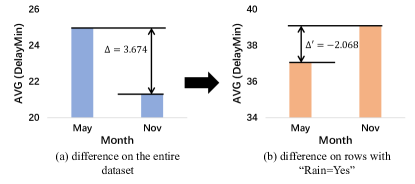
Figure 6. Explanation of Why Query on the FLIGHT dataset.

For the first Why Query, we observe that the duration of flight delay differs by month, particularly for May and November, which motivates us to ask XInsight for explanations — what the cause of the flight delay difference is. XInsight first learns a causal graph from data and identifies “rain” as a direct cause of DelayMinute. Then, XPlainer finds that the difference is reversed ($\Delta=3.674$ vs. $\Delta^{\prime}=-2.068$) when the condition “rain=Yes” is enforced (Fig. 6). Thus, it returns “rain=Yes” as an explanation. We interpret the explanation as correct because 1) rain is a typical reason for flight delay, and 2) for most states, monthly precipitation in May is usually higher than in November. Hence, when only counting the rainy cases (by enforcing “rain=Yes”), the difference is eliminated.

For the second Why Query, we observe that the cancellation rate varies by month of arrival. For instance, the cancellation rate in July is 0.37, which is higher than in January. Thus, we ask XInsight for explanations. XInsight identifies “LeadTime” (number of days between booking data and arrival date) as an indirect cause of “IsCanceled”. It also discovers that when enforcing “LeadTime$\leq 133$”, the difference is reduced. This is intuitive. A longer “LeadTime” results in greater uncertainty about guests’ future schedules, leading to a higher cancellation rate. In January, LeadTime of most reservations is less than 133 days (91%). In contrast, there are far more early reservations ($>133$ days) in July (48%), resulting in a higher cancellation rate. When these early reservations are excluded, the difference becomes much smaller.

Table 5. Results of explanation assessment. E$i$ and P$i$ stand for the $i$th explanation and the $i$th participant, respectively.

	E1	E2	E3	E4	E5	E6	E7	E8
P1	4	4	5	4	4	4	5	3
P2	4	4	4	4	3	4	3	4
P3	5	3	4	5	3	5	5	5
P4	3	4	5	4	4	3	3	4
P5	4	2	5	3	5	4	3	3
P6	5	4	5	5	5	4	5	5
mean	4.16	3.50	4.67	4.17	4.00	4.00	4.00	4.00
std	0.69	0.76	0.47	0.69	0.82	0.58	1.00	0.82

WEB. We report the results of the second phase in the user study (i.e., Explanation Assessment in Sec. 4.1) in Table 5. We view the results as encouraging, since nearly all responses are positive ($\geq 3$). Moreover, the average scores for seven out of eight explanations are $\geq 4$. We also investigated the explanation with the lowest score (E2 in Table 5). We find this is counter-intuitive but reasonable in retrospect. In the follow-up session, the discussion among participants also confirmed our finding. During the assessments, experts find many explanations inspiring and insightful, despite their familiarity with the dataset. It continuously increases their knowledge and help them design a better criteria for detecting malicious behavior.

Answer to RQ1: XInsight shows a promising end-to-end performance in explaining data differences. The user study validates that XInsight achieves a respectable level of agreement with experts.

4.3. RQ2: XLearner Evaluation

As a cornerstone of XInsight, XLearner is crucial to the effectiveness of the entire pipeline. To answer RQ2, we run XLearner on SYN-A which has ground truth causal graphs and on a real-world dataset WEB. Since WEB does not associate a ground-truth causal graph, we assess the quality of causal relations by the user study.

Table 6. Overall comparison between XLearner and FCI.

Algo.	F1-Score	Precision	Recall
XLearner	$0.88\pm 0.04$	$0.95\pm 0.03$	$0.82\pm 0.06$
FCI	$0.72\pm 0.05$	$0.92\pm 0.04$	$0.59\pm 0.06$

Table 6 provides an overall comparison between XLearner and FCI on SYN-A datasets. We find that XLearner is more accurate than FCI in the presence of FDs. In particular, while FCI has comparable precision, XLearner has a much higher recall. This confirms our discussion on the implications of FDs in Sec. 3.1. The faithfulness violations mislead FCI to incorrectly refute true edges (thus yield a lower recall) while XLearner is aware of such faithfulness violations and handles them with the procedure in Sec. 3.1.

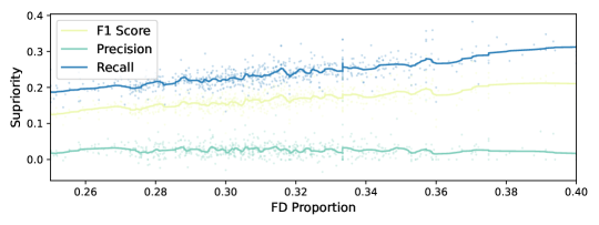
Figure 7. Comparison by FD Proportion. The x-axis is the proportion of FDs in the causal graph. The y-axis is the superiority (determined by subtracting the FCI’s score from the XLearner’s score) of XLearner over FCI.

Since XLearner focuses primarily on FDs as the opposite of FCI, we further study how varying proportions of FDs in the causal graph affect XLearner’s performance. We report the superiority in terms of varied amounts of FDs in Fig. 7. Overall, we observe an increasing trend in XLearner performance (particularly for F1 and recall) as the FD proportion increases. More importantly, we observe that “superiority” increases as FDs increase. Recall, as noted in the caption of Fig. 7, that the superiority is computed by subtracting the FCI’s score from the XLearner’s score. Thus, we interpret that XLearner gradually outperforms the FCI algorithm with greater degree as the proportion of FDs grows.

In addition to the experiments on synthetic datasets, we also evaluate XLearner with the WEB dataset (Sec. 4.1). As aforementioned, this real-world dataset lacks a ground-truth causal graph. Evaluating the accuracy of an estimated causal graph is thus challenging, if not impossible. At this step, we involve human experts to assess the correctness of the identified causal relations in the third phase of our user study (i.e., Causal Claim Assessment in Sec. 4.1).

Table 7. User study. C$i$ stands for the $i$th causal claim.

	C1	C2	C3	C4	C5	C6	C7	C8
# Reasonable	6	4	4	6	6	4	5	5
# Not Sure	0	2	1	0	0	0	1	1
# Not Reasonable	0	0	1	0	0	2	0	0

We report the results of our user study in Table 7: first, out of 48 responses ($6\text{~{}participants}~{}\times~{}8\text{~{}questions}$), only three ($6.3\%$) suggest that the causal claims are “Not Reasonable,” while $40$ responses ($83.3\%$) mark the causal claims as “Reasonable.” It indicates that the causal relations identified by XLearner correspond with expert knowledge in the majority of instances. Second, we investigate the claims that have been deemed “Not Reasonable” or “Unsure.” Encouragingly, we find that a notable proportion of causal claims are counter-intuitive yet correct. For instance, one causal claim states that “malicious intent would lead to more frequent configuration changes than benign intent.” In the causal claim assessment phase, one expert deemed it “Not Reasonable” and presumed that malicious users would keep a default configuration. In the follow-up session where they shared the independent assessments, this participant was persuaded and confirmed this causal relation as “Reasonable.”

Answer to RQ2: As reflected by the carefully-designed quantitative experiments and the user study, XLearner generates plausible causal graphs that are consistent with expert knowledge.

4.4. RQ3: XPlainer Evaluation

Recall the descriptions of SYN-B in which different parameters result in datasets with varying degrees of difficulty. In this experiment, we explore the accuracy of XPlainer on SYN-B.

Baseline. We compare XPlainer with three baselines, namely, Scorpion (wu2013scorpion, 54), RSExplain (roy2014formal, 47) and BOExplain (lockhart2021explaining, 27), which use predicates as explanations. Scorpion is an explanation engine for explaining outliers. It uses a metric called influence score to rank explanations, which considers the effect of the explanation between the outlier region and the hold-out region. RSExplain uses the concept of intervention to measure the effectiveness of an explanation. BOExplain is originally designed for explaining black-box machine learning models. When explaining Why Query, it employs the inference score and the Bayesian optimization to find the optimal explanation. To launch an apple-to-apple comparison, all baselines are enforced to search over a set of pre-defined causal filters $\{p_{1},\cdots,p_{m}\}$ derived from the generation procedure of SYN-B (see details in Supplementary Material); all these filters have been confirmed to constitute legitimate causal explanations.

Metric. We use the top-ranked explanation of each baseline as its optimal explanation. We mark a method as “N/A” denoting timeouts (more than one hour to process). We report the F1 Score of filters in the explanation over the ground-truth explanation.

Table 8. XPlainer and baselines under various settings. ✓ denotes that F1=1.0 and the best metric is highlighted.

#Rows (Cardinality=10)								10K	20K	50K	100K	500K	1M
XPlainer	F1 Score	✓	✓	✓	✓	✓	✓
(SUM)	Time (sec.)	0.004	0.005	0.007	0.010	0.017	0.019
Scorpion	F1 Score	0.5	0.5	0.5	0.5	0.5	0.8
(SUM)	Time (sec.)	0.68	0.82	1.25	1.93	2.45	2.93
RSExplain	F1 Score	0.75	0.75	0.75	0.75	0.75	0.75
(SUM)	Time (sec.)	0.68	0.83	1.25	1.94	2.44	2.90
BOExplain	F1 Score	0.8	0.8	0.5	0.5	0.5	0.8
(SUM)	Time (sec.)	5.24	5.32	5.62	6.38	9.80	13.53
XPlainer	F1 Score	✓	✓	✓	✓	✓	✓
(AVG)	Time (sec.)	0.016	0.019	0.026	0.038	0.052	0.063
Scorpion	F1 Score	✓	✓	✓	✓	✓	✓
(AVG)	Time (sec.)	0.59	0.67	0.90	1.29	1.69	2.01
RSExplain	F1 Score	0.75	0.75	0.75	0.75	0.75	0.75
(AVG)	Time (sec.)	0.58	0.66	0.90	1.28	1.68	1.95
BOExplain	F1 Score	0.86	✓	0.86	✓	✓	0.8
(AVG)	Time (sec.)	5.33	5.37	5.56	6.56	8.67	12.62
Cardinality (#Rows=100k)		10	15	20	30	50	100
XPlainer	F1 Score	✓	✓	✓	✓	✓	0.8
(SUM)	Time (sec.)	0.010	0.014	0.018	0.025	0.040	0.077
Scorpion	F1 Score	0.5	0.5	0.5	N/A	N/A	N/A
(SUM)	Time (sec.)	1.96	16.50	75.72	N/A	N/A	N/A
RSExplain	F1 Score	0.75	0.75	0.75	N/A	N/A	N/A
(SUM)	Time (sec.)	1.95	16.61	75.82	N/A	N/A	N/A
BOExplain	F1 Score	✓	0.86	0.86	0.46	0.27	0.15
(SUM)	Time (sec.)	6.28	8.71	11.17	15.44	25.44	48.73
XPlainer	F1 Score	✓	✓	✓	✓	✓	✓
(AVG)	Time (sec.)	0.038	0.060	0.082	0.124	0.211	0.426
Scorpion	F1 Score	✓	✓	✓	N/A	N/A	N/A
(AVG)	Time (sec.)	1.27	10.58	47.90	N/A	N/A	N/A
RSExplain	F1 Score	0.75	0.75	0.75	N/A	N/A	N/A
(AVG)	Time (sec.)	1.28	10.59	47.91	N/A	N/A	N/A
BOExplain	F1 Score	✓	0.86	0.5	0.5	0.27	0.14
(AVG)	Time (sec.)	5.87	8.23	10.44	15.00	24.35	46.35

Different Dataset Sizes. To study the scalability of XPlainer, we generate datasets of varying sizes and report the results in Table 8. Overall, we observe that XPlainer is more accurate and efficient than all baselines across all the studied settings. This is encouraging and also reasonable, as XPlainer uses many distinct characteristics of aggregation functions to optimize the search process, while other methods primarily treat them as a “black-box.” Scorpion and BOExplain often produce incomplete explanations, while RSExplain may frequently find extra spurious filters. We presume that this is because the objective function of Scorpion (and also BOExplain) is for explaining anomalies instead of Why Query, whereas RSExplain is primarily designed for data provenance. In contrast, explanations provided by XPlainer are seen as consistent with the ground truth.

XPlainer is highly efficient particularly for high cardinality regimes, while both Scorpion and RSExplain run out of time when the cardinality exceeds 30 (see the bottom half of Table 8). BOExplain uses Bayesian optimization to search for explanations, and its accuracy downgrades as cardinality increases. Similarly, when iterating different #Rows (the top half of Table 8), XPlainer also exhibits highly encouraging efficiency: XPlainer takes on average 0.06 seconds to explain Why Query whereas BOExplain (the second best) takes 13.17 seconds. In sum, we interpret from Table 8 that XPlainer delivers highly encouraging accuracy and efficiency across different settings in comparison with the baseline methods.

Different $\mu^{*}-\mu$. The difference between $\mu^{*},\mu$ indicates the magnitude of $\Delta$. To study the sensitivity of XPlainer, we study how well XPlainer performs under varying differences and compare it with baselines in Table 9. To clarify, $\mu^{*}-\mu=5$ and $\mu^{*}-\mu=10$ denote two relatively more challenging settings in Table 9, given the very subtle differences. On SUM aggregates, we find that all methods have difficulties in identifying explanations in those two challenging settings; still, XPlainer yields the best results for both settings. Even on the most challenging setting ($\mu^{*}-\mu=5$), XPlainer finds highly accurate explanations whereas RSExplain is less accurate.

Table 9. XPlainer and baselines with different $\mu^{*}-\mu$. ✓ denotes that the result is identical to the ground truth (F1=1.0).

$\mu-\mu^{*}$	5	10	15	30	50	100
XPlainer (SUM)	0.86	✓	✓	✓	✓	✓
Scorpion (SUM)	0.50	0.50	0.50	0.50	0.50	0.50
RSExplain (SUM)	0.75	0.75	0.75	0.75	0.75	0.75
BOExplain (SUM)	0.50	0.86	0.80	0.80	0.80	✓
XPlainer (AVG)	✓	✓	✓	✓	✓	✓
Scorpion (AVG)	0.80	✓	✓	✓	✓	✓
RSExplain (AVG)	0.75	0.75	0.75	0.75	0.75	0.75
BOExplain (AVG)	0.80	✓	0.86	0.86	0.80	✓

On AVG aggregates, XPlainer and Scorpion both perform well on identifying the ground-truth explanations; XPlainer is slightly better particularly for the most challenging setting when $\mu^{*}-\mu=5$. Nevertheless, RSExplain and BOExplain are less accurate on AVG. Overall, we conclude that XPlainer is more robust to subtle data differences while all other methods have difficulties in such challenging settings. We omit reporting the processing time here, since it has already been evidently explored in Table 8.

Tightness of Approximation. In Sec. 3.3, we show the approximation of minimal contingency for computing responsibilities under SUM and AVG. In the following, we compare the tightness of the responsibility $\hat{\rho}$ computed by $\overline{P}=P^{C}-P$ to the true responsibility $\rho$ computed by the minimal contingency $P_{\min}$ via brute-force search. The approximation error is computed as $E=\frac{|\hat{\rho}-\rho|}{\rho}$. Recall that we craft three filters that form the counterfactual cause in each dataset. In SUM, we can craft six ($3\choose 2$) actual causes from the three filters. In AVG, since the canonical predicate of AVG only supports the first $k$ filters as actual causes and the rest as contingencies, we pick the top-1 and top-2 filters as two actual causes and repeat the experiments on three datasets ($2\times 3$ in total). On the six actual causes of SUM aggregates, we find that the brute-force algorithm is $253.3\times$ slower than our approximated solution. More importantly, the approximation error is highly negligible with an average of $0.007$. We also observe that the approximation error on AVG is slightly higher ($0.066$) and that our heuristics-based solution is $27.3\times$ faster. This result is reasonable, as the heuristics-based solution does not provide guarantees of accuracy and requires more queries than SUM.

Answer to RQ3: XPlainer shows high scalability to large datasets and also accurately generates explanations in very difficult settings. On a mild cost of precision, two approximation solutions of XPlainer substantially improve efficiency.

5. Discussion

FD in Noisy Data. XInsight only considers deterministic FDs. As illustrated in Ex. 3.1, taking deterministic FDs into account eliminates faithfulness violations. However, when the data is noisy, the FDs may be stochastic (e.g., probabilistic interpretation of FDs (zhang2020statistical, 58)), which is currently not considered in XInsight. We clarify that considering only deterministic FDs deems a common setup shared by relevant works in this field (ding2020reliable, 12, 30). It remains unclear how noisy FDs may impact faithfulness. We leave this for future exploration.

Acquiring Causal Knowledge. Inferring causal relations is difficult. Typically, it needs a combination of domain knowledge (andrews2020completeness, 2), randomized experiments (triantafillou2015constraint, 52) and causal discovery (spirtes2000causation, 51, 57, 12, 29, 10). XInsight performs causal discovery from observational data due to its simplicity. Nevertheless, we envision users of XInsight can combine additional sources for acquiring more accurate causal knowledge. In this paper, we explain several key obstacles of applying causal discovery to real-world data, including causal insufficiency (zhang2008completeness, 57) and FD-induced faithfulness violations (ding2020reliable, 12, 30). XLearner, for the first time, simultaneously addresses all of them.

Other Forms of Explanations. Currently, XInsight employs predicates as the content of explanations, which is general enough for common data analysis scenarios. However, in some cases, explanations may be formed by the number of records in a database (tableau, 13) or counterbalances (miao2019going, 35). Furthermore, when explaining changes in a whole time series (chen2021tsexplain, 9), XInsight may be not applicable. We leave integrating XInsight into these scenarios for future work.

6. Related Work

Data Explanation. Explaining an unexpected query outcome in database is a crucial phase in the lifecycle of data analysis. In general, an explanation aims to provide certain forms of patterns that lead to the unexpected query outcome. Such patterns may be a set of predicates (wu2013scorpion, 54, 1, 4, 47), tuples (meliou2014causality, 31), or counterbalances (miao2019going, 35). Scorpion is the most relevant work for XInsight, which also provides explanations to aggregated queries (wu2013scorpion, 54). In particular, it employs an influence score to quantify explanations and features a set of optimizations to reduce the cost of explanation search. Recently, many tools have attempted to enhance explanations with additional knowledge (e.g., join tables) about the underlying data. However, such additional knowledge does not imply causation — top ranked explanations could be rated low by human participants due to a lack of causal semantics (li2021putting, 24). These observations evidently show the necessity of integrating causality into XDA.

Causality in Database. Most works related to causality analysis in the database is on the basis of Halpern’s seminal framework on actual causality (halpern2005causes, 19, 18). It provides an elegant and natural way to reason about input-output relations. Its results not only highlight the output’s cause, but also provide a contingency describing how it is triggered. The adaption of actual causality in the database (i.e., DB causality) is widely used for data provenance (meliou2010complexity, 33), data explanation (roy2014formal, 47) and debugging (meliou2011tracing, 34, 14, 56, 20). However, it has limitations when applied alone. On the one hand, as noted in (glavic2021trends, 17), DB causality does not necessarily imply true causation. Indeed, it assumes that causal knowledge is already known, and focuses solely on quantitative explanations. On the other hand, considerable adaptions are required to make it applicable to XDA scenarios, as discussed in Sec. 3.3. We also notice other methods for quantifying explanations, such as sufficient score, necessity score, and average causal effect (salimi2020causal, 48, 53). Despite their usefulness, we design XPlainer on top of actual causality because it is more understandable and general. Furthermore, without prior causal knowledge, none of these methods can imply true causation.

XDA vs. XAI. We note that XAI (explainable artificial intelligence) is parallel and complementary to XDA. Through the lens of data analysis, XAI aims to explain a prediction or model (pradhan2022explainable, 46, 16), while XDA enhances EDA for understanding data facts. In addition, we also observe a line of research (wu2020complaint, 55, 15, 26, 25) that identifies a subset of (training) data that is responsible for a prediction. While this line of research shares similar output format with XInsight, it is essentially for explaining how model predictions are influenced by training/test data, a scenario that is orthogonal to our research.

7. Conclusion

This paper advocates XDA, a concept that ships comprehensive and in-depth explainability toward EDA. XDA offers either causal or non-causal explanations for EDA outcomes, from both quantitative and qualitative perspectives. We have also presented the design of XInsight, a production framework for XDA over databases. Experiments and human evaluations reveal that XInsight manifests highly encouraging explanation capabilities. XPlainer has been integrated into Microsoft Power BI to explain increase/decrease in data.

8. Supplementary Material

8.1. Fast Causal Inference (FCI) Algorithm (spirtes2000causation, 51, 57)

We first introduce concepts and notations in addition to the one described in Sec. 2.2. Then, we outline the FCI algorithm in Alg. 3 and Alg. 4.

Definition 8.0 (Unshielded Triple).

In a graph, a triple $(X,Y,Z)$ is an unshielded triple if $X$ and $Z$ are non-adjacent, $X$ and $Z$ are adjacent, and $Y$ and $Z$ are adjacent.

Definition 8.0 (Possible-D-SEP).

In a graph, $\textit{Possible-D-SEP}(X,Y)$ is the set of nodes $Z$ such that there is an undirected path $\mathcal{P}$ between $X$ and $Z$ and for each subpath $S{*\hskip 0.85358pt\!\!\!-\hskip 0.85358pt\!\!\!*}W{*\hskip 0.85358pt\!\!\!-\hskip 0.85358pt\!\!\!*}T$ of $\mathcal{P}$ one of the following conditions holds.

1. $W$ is a collider; or,

2. $W$ is not marked as a non-collider and $S,W,T$ are a triangle. (A triangle is a set of three nodes all adjacent to one another).

Definition 8.0 (Ext-D-SEP).

In a graph, $\textit{Ext-D-SEP}(X,Y)$ is the union of $\textit{Possible-D-SEP}(X,Y)$ and $\textit{Possible-D-SEP}(Y,X)$.

Definition 8.0 (Discriminating Path).

In a MAG, a path between $X$ and $Y$, $\mathcal{P}=(X,\cdots,W,V,Y)$, is a discriminating path for $V$ if

1. $\mathcal{P}$ includes at least three edges;

2. $V$ is a non-endpoint node on $\mathcal{P}$, and is adjacent to $Y$ on $\mathcal{P}$; and

3. $X$ is not adjacent to $Y$, and every node between $X$ and $V$ is a collider on $\mathcal{P}$ and is a parent of $Y$.

Definition 8.0 (Uncovered Path).

In a PMG (partial mixed graph), a path $\mathcal{P}=(V_{0},\cdots,V_{n})$ is said to be uncovered if for every $1\leq i\leq n-1$, $V_{i-1}$ and $V_{i+1}$ are not adjacent, i.e., if every consecutive triple on the path is unshielded.

Definition 8.0 (Potentially Directed Path).

In a PMG (partial mixed graph), a path $\mathcal{P}=(V_{0},\cdots,V_{n})$ is said to be potentially directed (abbreviated as p.d.) from $V_{0}$ to $V_{n}$ if for every $0\leq i\leq n-1$, the edge between $V_{i}$ and $V_{i+1}$ is not into $V_{i}$ or out of $V_{i+1}$.

Definition 8.0 (Circle Path).

In a PMG (partial mixed graph), a circle path $\mathcal{P}=(V_{0},\cdots,V_{n})$ is a special case of p.d. path, where each edge on $\mathcal{P}$ is ${\circ\hskip 1.13809pt\!\!\!-\hskip 1.13809pt\!\!\!\circ}$.

Input: Data $D$

Output: Skeleton $G$

1 initialize a complete undirected graph $Q$ with $n$ nodes;

2 $n\leftarrow 0$;

3

4repeat

5      

6      repeat

7             select an ordered pair of adjacent nodes $X,Y$ such that $\textit{Neighbor}(X)\setminus\{Y\}$ has cardinality $\geq n$, and a subset $\bm{S}\subseteq\textit{Neighbor}(X)\setminus\{Y\}$ of cardinality $n$, and, if $X\Perp Y\mid S$, delete the edge between $X$ and $Y$ from $Q$, and record $\bm{S}$ in $\textit{Sepset}(X,Y)$ and $\textit{Sepset}(Y,X)$;

8      until all ordered pairs of adjacent nodes $X$ and $Y$ such that $\textit{Neighbor}(X)\setminus\{Y\}$ has cardinality $\geq n$ and all subsets $\bm{S}$ in $\textit{Neighbor}(X)\setminus\{Y\}$ have been tested for d-separation;

9      $n\leftarrow n+1$;

10      

11until for each ordered pair of adjacent nodes $X,Y$, $\textit{Neighbor}(X)\setminus\{Y\}$ has less than $n$ neighbors;

12let $F^{\prime}$ be the undirected graph from the above step and orient each edge as ${\circ\hskip 1.13809pt\!\!\!-\hskip 1.13809pt\!\!\!\circ}$;

13 foreach unshielded triple $(X,Y,Z)\in F^{\prime}$ do

14       if $Y$ is not in $\textit{Sepset}(X,Z)$ then

15             orient $X{*\hskip 0.85358pt\!\!\!-\hskip 0.85358pt\!\!\!*}Y{*\hskip 0.85358pt\!\!\!-\hskip 0.85358pt\!\!\!*}Z$ as $X{*\hskip 0.85358pt\!\!\!\rightarrow}Y{\leftarrow\hskip 0.85358pt\!\!\!*}Z$;

16            

17       end if

18      

19 end foreach

20foreach adjacent pair $(X,Y)\in F^{\prime}$ do

21       if there exists a subset $\bm{S}\subseteq\textit{Ext-D-SEP}(X,Y)$ such that $X\Perp Y\mid\bm{S}$ then

22             delete the edge between $X$ and $Y$ from $F^{\prime}$;

23            

24       end if

25      

26 end foreach

27let $G$ be the undirected graph of $F^{\prime}$;

return $G,\textit{Sepset}$

Algorithm 3 FCI-SL

Input: Skeleton $S$, Sepset Sepset

Output: PAG $G$

1

2let $G$ be the graph sharing all adjacencies of $S$ and orient each edge as ${\circ\hskip 1.13809pt\!\!\!-\hskip 1.13809pt\!\!\!\circ}$;

3 foreach unshielded triple $(\alpha,\beta,\gamma)\in G$ do

4       if $\beta$ is not in $\textit{Sepset}(\alpha,\gamma)$ then

5             orient $\alpha{*\hskip 0.85358pt\!\!\!-\hskip 0.85358pt\!\!\!*}\beta{*\hskip 0.85358pt\!\!\!-\hskip 0.85358pt\!\!\!*}\gamma$ as $\alpha{*\hskip 0.85358pt\!\!\!\rightarrow}\beta{\leftarrow\hskip 0.85358pt\!\!\!*}\gamma$;

6            

7       end if

8      

9 end foreach

10repeat

11      

12      $\mathcal{R}1$: if $\alpha{*\hskip 0.85358pt\!\!\!\rightarrow}\beta{\circ\!-\hskip 0.85358pt\!\!\!*}\gamma$, and $\alpha$ and $\gamma$ are not adjacent, then orient the triple as $\alpha{*\hskip 0.85358pt\!\!\!\rightarrow}\beta\rightarrow\gamma$;

13      

14      $\mathcal{R}2$: if $\alpha\rightarrow\beta{*\hskip 0.85358pt\!\!\!\rightarrow}\gamma$ or $\alpha{*\hskip 0.85358pt\!\!\!\rightarrow}\beta\rightarrow\gamma$, and $\alpha{*\hskip 0.85358pt\!\!\!-\hskip 0.85358pt\!\!\!\circ}\gamma$, then orient $\alpha{*\hskip 0.85358pt\!\!\!-\hskip 0.85358pt\!\!\!\circ}\gamma$ as $\alpha{*\hskip 0.85358pt\!\!\!\rightarrow}\gamma$;

15      

16      $\mathcal{R}3$: if $\alpha{*\hskip 0.85358pt\!\!\!\rightarrow}\beta{\leftarrow\hskip 0.85358pt\!\!\!*}\gamma$, $\alpha{*\hskip 0.85358pt\!\!\!-\hskip 0.85358pt\!\!\!\circ}\theta{\circ\!-\hskip 0.85358pt\!\!\!*}\gamma$, and $\alpha$ and $\gamma$ are not adjacent, and $\theta{*\hskip 0.85358pt\!\!\!-\hskip 0.85358pt\!\!\!\circ}\beta$, then orient $\theta{*\hskip 0.85358pt\!\!\!-\hskip 0.85358pt\!\!\!\circ}\beta$ as $\theta{*\hskip 0.85358pt\!\!\!\rightarrow}\beta$;

17      

18      $\mathcal{R}4$: if $u=(\theta,\cdots,\alpha,\beta,\gamma)$ is a discriminating path between $\theta$ and $\gamma$ for $\beta$, and $\beta{\circ\!-\hskip 0.85358pt\!\!\!*}\gamma$; then if $\beta\in\textit{Sepset}(\theta,\gamma)$, orient $\beta{\circ\!-\hskip 0.85358pt\!\!\!*}\gamma$ as $\beta\rightarrow\gamma$; otherwise orient the triple $(\alpha,\beta,\gamma)$ as $\alpha\leftrightarrow\beta\leftrightarrow\gamma$;

19      

20until none of the orientation rules applies;

21repeat

22      

23      $\mathcal{R}5$: for every (remaining) $\alpha{\circ\hskip 1.13809pt\!\!\!-\hskip 1.13809pt\!\!\!\circ}\beta$, if there is an uncovered circle path $p=(\alpha,\gamma,\cdots,\theta,\beta)$ between $\alpha$ and $\beta$ s.t. $\alpha$ and $\beta$ are not adjacent, and $\gamma$ and $\theta$ are not adjacent, then orient $\alpha{\circ\hskip 1.13809pt\!\!\!-\hskip 1.13809pt\!\!\!\circ}\beta$ and every edge on $p$ as undirected edges (—);

24      

25      $\mathcal{R}6$: if $\alpha-\beta{\circ\!-\hskip 0.85358pt\!\!\!*}\gamma$ ($\alpha$ and $\gamma$ may or may not be adjacent), then orient $\beta{\circ\!-\hskip 0.85358pt\!\!\!*}\gamma$ as $\beta{-\hskip 0.85358pt\!\!\!*}\gamma$;

26      

27      $\mathcal{R}7$: if $\alpha-\beta{\circ\!-\hskip 0.85358pt\!\!\!*}\gamma$ , and $\alpha$ and $\gamma$ are not adjacent, then orient $\beta{\circ\!-\hskip 0.85358pt\!\!\!*}\gamma$ as $\beta{-\hskip 0.85358pt\!\!\!*}\gamma$;

28      

29      $\mathcal{R}8$: if $\alpha\rightarrow\beta\rightarrow\gamma$ or $\alpha{-\hskip 0.85358pt\!\!\!\circ}\beta\rightarrow\gamma$, and $\alpha{\circ\hskip 0.85358pt\!\!\!\rightarrow}\gamma$, orient $\alpha{\circ\hskip 0.85358pt\!\!\!\rightarrow}\gamma$ as $\alpha\rightarrow\gamma$;

30      

31      $\mathcal{R}9$: if $\alpha{\circ\hskip 0.85358pt\!\!\!\rightarrow}\gamma$ and $p=(\alpha,\beta,\theta,\cdots,\gamma)$ is an uncovered p.d. path from $\alpha$ to $\gamma$ such that $\beta$ and $\gamma$ are not adjacent, then orient $\alpha{\circ\hskip 0.85358pt\!\!\!\rightarrow}\gamma$ as $\alpha\rightarrow\gamma$;

32      

33      $\mathcal{R}10$: suppose $\alpha{\circ\hskip 0.85358pt\!\!\!\rightarrow}\gamma$, $\beta\rightarrow\gamma\leftarrow\theta$, $p_{1}$ is an uncovered p.d. path from $\alpha$ to $\beta$ and $p_{2}$ is an uncovered p.d. path from $\alpha$ to $\theta$. Let $\mu$ be the node adjacent to $\alpha$ on $p_{1}$ ($\mu$ could be $\beta$), and $\omega$ be the node adjacent to $\alpha$ on $p_{2}$ ($\omega$ could be $\theta$). If $\mu$ and $\omega$ are distinct, and are not adjacent, then orient $\alpha{\circ\hskip 0.85358pt\!\!\!\rightarrow}\gamma$ as $\alpha\rightarrow\gamma$;

34      

35until none of the orientation rules applies;

36return $G$

Algorithm 4 FCI-Orient

8.2. Principle of Explainability under AVG and SUM

In AVG, we notice that $\color[rgb]{0,0,0}\texttt{AVG}_{M}(s_{1})\approx\mathbb{E}(M\mid F=f_{1})$ and $\color[rgb]{0,0,0}\texttt{AVG}_{M}(s_{2})\approx\mathbb{E}(M\mid F=f_{2})$ asymptotically. $\color[rgb]{0,0,0}\texttt{AVG}_{M}(s_{1}\land X=x)\approx\mathbb{E}(M\mid F=f_{1},X=x)=\mathbb{E}(M\mid F=f_{1})=\texttt{AVG}_{M}(s_{1})$. Similarly, $\color[rgb]{0,0,0}\texttt{AVG}_{M}(s_{2}\land X=x)\approx\texttt{AVG}_{M}(s_{1})$. Hence, $\color[rgb]{0,0,0}\Delta(D)\approx\Delta(D_{X=x})$.

In SUM, we notice that $\color[rgb]{0,0,0}\texttt{SUM}=\texttt{COUNT}\times\texttt{AVG}$ and $\color[rgb]{0,0,0}\texttt{COUNT}_{M}(s_{1})=N\times P(F=f_{1}),\texttt{COUNT}_{M}(s_{2})=N\times P(F=f_{2})$, where $\color[rgb]{0,0,0}N$ is a constant indicating the number of rows in the data. Then, $\color[rgb]{0,0,0}\Delta=N(P(F=f_{1})\mathbb{E}(M\mid F=f_{1})-P(F=f_{2})\mathbb{E}(M\mid F=f_{2}))$. $\color[rgb]{0,0,0}\Delta(D_{X=x})=N(P(F=f_{1},X=x)\mathbb{E}(M\mid F=f_{1},X=x)-P(F=f_{2},X=x)\mathbb{E}(M\mid F=f_{2},X=x))=N(P(F=f_{1},X=x)\mathbb{E}(M\mid F=f_{1})-P(F=f_{2},X=x)\mathbb{E}(M\mid F=f_{2}))$.

8.3. Proof of Thm. 3.4

Lemma 8.3.0.

If $\color[rgb]{0,0,0}X\xrightarrow{\texttt{FD}}Y$, then $\color[rgb]{0,0,0}Y\not\!\perp\!\!\!\perp X$, and for any other variable set $\color[rgb]{0,0,0}Z$, $\color[rgb]{0,0,0}Z\Perp Y\mid X$.

Proof.

Because $\color[rgb]{0,0,0}X\xrightarrow{\texttt{FD}}Y$, $\color[rgb]{0,0,0}P(Y\mid X)=I_{Y=f(X)}$. Since $\color[rgb]{0,0,0}|X|,|Y|>1$, the following inequality holds.

(9) $$P(XY)=P(X)P(Y\mid X)=P(X)I_{Y=f(X)}\neq P(X)P(Y)$$

Therefore, $\color[rgb]{0,0,0}Y\not\!\perp\!\!\!\perp X$. Given a variable set $\color[rgb]{0,0,0}Z$,

(10) $$P(YZ\mid X) =\frac{P(XYZ)}{P(X)}$$

$$=\frac{P(XZ)I_{Y=f(X)}}{P(X)}$$

$$=P(Z\mid X)I_{Y=f(X)}$$

$$=P(Z\mid X)P(Y\mid X)$$

Therefore, $\color[rgb]{0,0,0}Z\Perp Y\mid X$. ∎

Lemma 8.3.0.

If $\color[rgb]{0,0,0}X\xrightarrow{\texttt{FD}}Y$ and $\color[rgb]{0,0,0}Z\Perp X\mid W$, then $\color[rgb]{0,0,0}Z\Perp Y\mid W$, where $\color[rgb]{0,0,0}Z$ and $\color[rgb]{0,0,0}W$ are two disjoint variable set other than $\color[rgb]{0,0,0}X$ and $\color[rgb]{0,0,0}Y$.

Proof.

Let $\color[rgb]{0,0,0}\pi_{y}=\{x\mid f(x)=y\}$. Therefore, $\color[rgb]{0,0,0}\{X\in\pi_{y}\}=\{Y=y\}$. Since $\color[rgb]{0,0,0}Z\Perp X\mid W$,

(11) $$P(Y=y,Z\mid W) =P(X\in\pi_{y},Z\mid W)$$

$$=P(X\in\pi_{y}\mid W)P(Z\mid W)$$

$$=P(Y=y\mid W)P(Z\mid W)$$

Therefore, $\color[rgb]{0,0,0}Z\Perp Y\mid W$. ∎

Lemma 8.3.0.

In a MAG $\color[rgb]{0,0,0}\mathcal{G}$ over variables $\color[rgb]{0,0,0}\{X_{1},\cdots,X_{n}\}$, if $\color[rgb]{0,0,0}X_{1}\rightarrow X_{2}$ and no other edges connect $\color[rgb]{0,0,0}X_{2}$ with other vertices, when $\color[rgb]{0,0,0}X_{2}{\Perp_{\mathcal{G}}}Y\mid U$ for any $\color[rgb]{0,0,0}Y\in\{X_{3},\cdots,X_{n}\},U\subset\{X_{3},\cdots,X_{n}\},Y\notin U$, $\color[rgb]{0,0,0}X_{1}{\Perp_{\mathcal{G}}}Y\mid U$.

Proof.

If $\color[rgb]{0,0,0}X_{2}{\Perp_{\mathcal{G}}}Y\mid U$, according to the definition of m-separation, each path between $\color[rgb]{0,0,0}X_{2}$ and $\color[rgb]{0,0,0}Y$ satisfies one of the following two conditions: 1) there exists $\color[rgb]{0,0,0}X_{p}\rightarrow X_{s}\rightarrow X_{q}$, $\color[rgb]{0,0,0}X_{p}\leftarrow X_{s}\rightarrow X_{q}$, or $\color[rgb]{0,0,0}X_{p}\leftarrow X_{s}\leftarrow X_{q}$ where $\color[rgb]{0,0,0}X_{s}\in U$. 2) there exists $\color[rgb]{0,0,0}X_{p}\rightarrow X_{s}\leftarrow X_{q}$ where $\color[rgb]{0,0,0}X_{s}$ or any of its descendants does not belong to $\color[rgb]{0,0,0}U$. Because $\color[rgb]{0,0,0}X_{1}\notin U$, $\color[rgb]{0,0,0}X_{1}\neq X_{s}$. For the first case, $\color[rgb]{0,0,0}X_{s}$ blocks $\color[rgb]{0,0,0}X_{1}$ and $\color[rgb]{0,0,0}Y$ given that there is only one edge connecting to $\color[rgb]{0,0,0}X_{2}$. For the second case, $\color[rgb]{0,0,0}X_{1}$ cannot be a collider, because $\color[rgb]{0,0,0}X_{1}\rightarrow X_{2}$. Therefore, $\color[rgb]{0,0,0}U$ also blocks $\color[rgb]{0,0,0}X_{1}$ and $\color[rgb]{0,0,0}Y$ on this path. In summary, $\color[rgb]{0,0,0}X_{1}{\Perp_{\mathcal{G}}}Y\mid U$. ∎

With above lemmas, now we prove Thm. 3.4.

Proof.

We first construct a MAG $\color[rgb]{0,0,0}\mathcal{G}$ on the top of the skeleton, by adding an arrowhead from $\color[rgb]{0,0,0}X_{1}$ to $\color[rgb]{0,0,0}Z$ ($\color[rgb]{0,0,0}\mathcal{G}_{2}$). Because $\color[rgb]{0,0,0}\mathcal{S}_{1}$ is learnt from $\color[rgb]{0,0,0}\{X_{1},\cdots,X_{n}\}$ where faithfulness assumption holds, this part is harmonious. For $\color[rgb]{0,0,0}Z$, there are two types of m-separation in $\color[rgb]{0,0,0}\mathcal{G}$. Here, we prove that each type of m-separation satisfies GMP to data distribution $\color[rgb]{0,0,0}P_{V}$.

Type 1: $\color[rgb]{0,0,0}Z{\Perp_{\mathcal{G}}}X_{j\neq 1}\mid X_{1}$

According to Lemma. 8.8, $\color[rgb]{0,0,0}X_{1}\xrightarrow{\texttt{FD}}Z$ implies that $\color[rgb]{0,0,0}Z\Perp X_{j\neq 1}\mid X_{1}$.

Type 2: $\color[rgb]{0,0,0}Z{\Perp_{\mathcal{G}}}X_{j}\mid U(j\neq 1,U\cap\{X_{1},X_{j}\}=\emptyset)$

By Lemma. 8.10, $\color[rgb]{0,0,0}Z{\Perp_{\mathcal{G}}}X_{j}\mid U$ implies that $\color[rgb]{0,0,0}X_{1}{\Perp_{\mathcal{G}}}X_{j}\mid U$. Because $\color[rgb]{0,0,0}S_{1}$ is harmonious, $\color[rgb]{0,0,0}X_{1}{\Perp_{\mathcal{G}}}X_{j}\mid U$ implies that $\color[rgb]{0,0,0}X_{1}\Perp X_{j}\mid U$. According to Lemma. 8.9, $\color[rgb]{0,0,0}X_{1}\xrightarrow{\texttt{FD}}Z$ and $\color[rgb]{0,0,0}X_{1}\Perp X_{j}\mid U$ imply $\color[rgb]{0,0,0}Z\Perp X_{j}\mid U$.

Minimality is satisfied, since removing edge from $\color[rgb]{0,0,0}X_{1}$ to $\color[rgb]{0,0,0}Z$ will make $\color[rgb]{0,0,0}X_{1}\Perp Z$ which contradicts $\color[rgb]{0,0,0}P_{V}$. ∎

8.4. Proof of Thm. 3.6

Proof.

We prove Thm. 3.6 by mathematical induction. In the sense, Alg. 1 returns a harmonious skeleton when $\color[rgb]{0,0,0}\mathcal{G}_{\texttt{FD}}$ has arbitrary number of non-root vertices. Denote the number of non-root vertices as $\color[rgb]{0,0,0}s\geq 0$.

Base Case. When $\color[rgb]{0,0,0}s=0$, the skeleton is harmonious because all variables are under faithfulness assumptions.

Induction. Suppose the returned skeleton is harmonious for $\color[rgb]{0,0,0}\mathcal{G}_{\texttt{FD}}$ when $\color[rgb]{0,0,0}s=n$. Now we prove the skeleton is still harmonious when we add a vertex $\color[rgb]{0,0,0}X^{\prime}$ to a vertex set $\color[rgb]{0,0,0}\bm{X}\subseteq\mathcal{G}_{\texttt{FD}}.V$. Denote the new FD-induced graph as $\color[rgb]{0,0,0}\mathcal{G}_{\texttt{FD}}^{\prime}$, the skeleton of $\color[rgb]{0,0,0}\mathcal{G}_{\texttt{FD}}$ as $\color[rgb]{0,0,0}\mathcal{S}$, and the skeleton for $\color[rgb]{0,0,0}\mathcal{G}_{\texttt{FD}}^{\prime}$ as $\color[rgb]{0,0,0}\mathcal{S}^{\prime}$. According to Alg. 1, $\color[rgb]{0,0,0}\mathcal{S},\mathcal{S}^{\prime}$ share the same vertices and edges (except $\color[rgb]{0,0,0}X^{\prime}$). Given that $\color[rgb]{0,0,0}\mathcal{S}$ is harmonious, $\color[rgb]{0,0,0}\mathcal{S}^{\prime}$ can be decomposed into two subgraphs, i.e., $\color[rgb]{0,0,0}\mathcal{S}_{1},\mathcal{S}_{2}$, where $\color[rgb]{0,0,0}\mathcal{S}_{1}=\mathcal{S}$ and $\color[rgb]{0,0,0}\mathcal{S}_{2}$ corresponds to $\color[rgb]{0,0,0}X^{\prime}$ and one edge from $\color[rgb]{0,0,0}X^{\prime}$ to one of $\color[rgb]{0,0,0}\bm{X}$. Since $\color[rgb]{0,0,0}X^{\prime\prime}\xrightarrow{\texttt{FD}}X^{\prime}$, by Thm. 3.4, $\color[rgb]{0,0,0}\mathcal{S}^{\prime}$ is harmonious.

By the principle of mathematical induction, Thm. 3.6 holds.

∎

8.5. FCI Rules on FD-related Edges

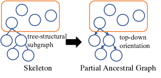
Figure 8. Orientation on tree-structural subgraph.

Since we only consider one-to-one and one-to-many FDs, FD-induced vertices only have at most one parent node in $\color[rgb]{0,0,0}\mathcal{G}_{\texttt{FD}}$. Therefore, it forms tree-structural subgraphs in the skeleton starting from the root vertices of $\color[rgb]{0,0,0}\mathcal{G}_{\texttt{FD}}$ (e.g., the left-hand side skeleton shown in Fig. 8). Intuitively, it would be ideal if the orientation rules allow us to orient the tree-structural subgraphs in a top-down manner (e.g., the right-hand side of Fig. 8). In particular, if there is an edge heading to the root node of the tree-structural subgraph, we can assign $\color[rgb]{0,0,0}\rightarrow$ ($\color[rgb]{0,0,0}\rightarrow$ is defined in Table 1) as the edge from the root node to its child vertices and propagate the directions to the leaf node by applying Rule 1 of FCI recursively.

Definition 8.0 (Rule 1 of FCI (zhang2008completeness, 57)).

If $\color[rgb]{0,0,0}X{*\hskip 0.85358pt\!\!\!\rightarrow}Y{\circ\hskip 0.85358pt\!\!\!\rightarrow}Z$ and $\color[rgb]{0,0,0}X,Z$ are non-adjacent, then orient $\color[rgb]{0,0,0}Y\rightarrow Z$. 

However, it is not necessarily attainable if we cannot identify the direction on the edge heading to the root node (i.e., $\color[rgb]{0,0,0}Y$ in Def. 8.11). As a result, we cannot derive any directions on the subgraphs. That is, all edges on the subgraph are $\color[rgb]{0,0,0}$, which denote edges with unknown directions. Such ambiguous cases are surely undesirable in XDA scenarios.

8.6. ANM on FD-related Edges

We note that, from viewpoint of conditional independence, functional dependency does not imply causal directions in all cases. However, we present that the counterexamples of such cases (i.e., contrasting direction between causal relation and functional dependency) are very rare in practice, if at all possible. Recall the theorem of “Identifiability of discrete ANMs” in (peters2017elements, 43).

Theorem 8.12.

Assume that a distribution $\color[rgb]{0,0,0}P_{X,Y}$ allows for an ANM $\color[rgb]{0,0,0}Y=f(X)+N_{Y}$ from $\color[rgb]{0,0,0}X$ to $\color[rgb]{0,0,0}Y$ and that either $\color[rgb]{0,0,0}X$ or $\color[rgb]{0,0,0}Y$ has finite support. $\color[rgb]{0,0,0}P_{X,Y}$ allows for an ANM from $\color[rgb]{0,0,0}Y$ to $\color[rgb]{0,0,0}X$ if and only if there exists a disjoint decomposition $\color[rgb]{0,0,0}\bigcup_{i=0}^{l}C_{i}=\text{supp}X$, such that the following conditions a), b), and c) are satisfied:

a) The $\color[rgb]{0,0,0}C_{i}$’s are shifted versions of each other

(12) $$\forall i\exists d_{i}>0:C_{i}=C_{0}+d_{i}$$

and $\color[rgb]{0,0,0}f$ is piecewise constant: $\color[rgb]{0,0,0}f\mid C_{i}\equiv c_{i}\forall i$.

b) The probability distributions on the $\color[rgb]{0,0,0}C_{i}$s are shifted and scaled versions of each other with the same shift constant as above: For $\color[rgb]{0,0,0}x\in C_{i}$, $\color[rgb]{0,0,0}P(X=x)$ satisfies

(13) $$P(X=x)=P(X=x-d_{i})\cdot\frac{P(x\in C_{i})}{P(x\in C_{0})}$$

c) The sets $\color[rgb]{0,0,0}c_{i}+\text{supp}N_{Y}:=\{c_{i}+h:P(N_{Y}=h)>0\}$ are disjoint sets.

By condition c), since $\color[rgb]{0,0,0}N_{Y}=0$ by functional dependency, $\color[rgb]{0,0,0}\nexists x_{i}\in C_{i},x_{j}\in C_{j}$ s.t. $\color[rgb]{0,0,0}f(x_{i})=f(x_{j})$. In other word, $\color[rgb]{0,0,0}X$ are decomposed by the value of $\color[rgb]{0,0,0}f(x)$ and each $\color[rgb]{0,0,0}c_{i}\in f(X)$ forms a disjoint subset $\color[rgb]{0,0,0}C_{i}$ of $\color[rgb]{0,0,0}X$. To admit condition a), each $\color[rgb]{0,0,0}C_{i}$ is a shifted version of others. Therefore, each $\color[rgb]{0,0,0}C_{i}$ should at least have an equal cardinality. The above two conditions imply that each $\color[rgb]{0,0,0}y\in Y$ corresponds to equal size of $\color[rgb]{0,0,0}x\in X$. Consider the aforementioned example where $\color[rgb]{0,0,0}\text{Country}\xrightarrow{\texttt{FD}}\text{Continent}$. To satisfy the condition, each continent must have equal number of countries. Furthermore, by condition b), the probability of a country $\color[rgb]{0,0,0}x$ in continent $\color[rgb]{0,0,0}c_{i}$ in the database can be exactly scaled by $\color[rgb]{0,0,0}\frac{P(x\in C_{i})}{P(x\in C_{0})}$ the probability of another shifted country $\color[rgb]{0,0,0}x-d_{i}$. The conditions together exhibits a very rare scenario. Therefore, we ignore such cases in practice.

As consistent with (peters2017elements, 43), we consider it reasonable to infer that direction of ANM as causal. Therefore, we hypothesis that functional dependencies in $\color[rgb]{0,0,0}\mathcal{G}_{\texttt{FD}}$ intrinsically imply causal directions.

8.7. Proof of Proposition 3.14

Proof.

Suppose there exists an optimal explanation $\color[rgb]{0,0,0}P^{*}$ such that $\color[rgb]{0,0,0}\exists p_{i}\in P^{*},\Delta_{i}\leq 0$. Let $\color[rgb]{0,0,0}P^{\prime}=\{p\mid p\in P^{*},\Delta_{p}>0\}$ and $\color[rgb]{0,0,0}\Gamma$ be the minimal contingency of $\color[rgb]{0,0,0}P^{*}$.

For SUM, since $\color[rgb]{0,0,0}\Delta(D_{P^{\prime}})\geq\Delta(D_{P^{*}})$, $\color[rgb]{0,0,0}\Delta(D)-\Delta(D_{\Gamma})-\Delta(D_{P^{\prime}})<\Delta(D)-\Delta(D_{\Gamma})-\Delta(D_{P^{*}})\leq\epsilon$.

For homogeneous AVG,

(14) $$\Delta(D-\Gamma-P^{\prime}) =\frac{\sum_{p_{i}\in\{p_{1},\cdots,p_{m}\}-\Gamma-P^{\prime}}a_{i}\Delta_{i}}{A_{D-\Gamma-P^{\prime}}}$$

$$<\frac{\sum_{p_{i}\in\{p_{1},\cdots,p_{m}\}-\Gamma-P^{*}}a_{i}\Delta_{i}}{A_{D-\Gamma-P^{*}}}$$

$$=\Delta(D-\Gamma-P^{*})\leq\epsilon$$

Hence, $\color[rgb]{0,0,0}\Gamma$ is also a valid contingency for $\color[rgb]{0,0,0}P^{\prime}$. $\color[rgb]{0,0,0}\rho_{P^{\prime}}\geq\rho_{P^{*}}$ and $\color[rgb]{0,0,0}|P^{\prime}|<|P^{*}|$ contradict the fact that $\color[rgb]{0,0,0}P^{*}$ is optimal. ∎

8.8. Proof of Proposition 3.16

Proof.

When there are more than one optimal explanations, let $\color[rgb]{0,0,0}P^{\prime}$ be the one with the smallest predicate size (i.e., $\color[rgb]{0,0,0}|P|$) and $\color[rgb]{0,0,0}\Gamma^{\prime}$ be the corresponding minimal contingency. Otherwise, let $\color[rgb]{0,0,0}P^{\prime}$ and $\color[rgb]{0,0,0}\Gamma^{\prime}$ be the optimal explanation and corresponding minimal contingency, respectively. If $\color[rgb]{0,0,0}|P^{\prime}|\geq|P^{C}|$, given that $\color[rgb]{0,0,0}\rho_{P^{\prime}}\leq 1$ and $\color[rgb]{0,0,0}\rho_{P^{C}}=1$, $\color[rgb]{0,0,0}\rho_{P^{\prime}}-\sigma\rho_{P^{\prime}}\leq\rho_{P^{C}}-\sigma\rho_{P^{C}}$. $\color[rgb]{0,0,0}P^{C}$ is at least as optimal as $\color[rgb]{0,0,0}P^{\prime}$. If $\color[rgb]{0,0,0}|P^{\prime}|<|P^{C}|$, then let $\color[rgb]{0,0,0}P^{\prime\prime}$ be a predicate by replacing all non-canonical filters in $\color[rgb]{0,0,0}P^{\prime}$ with canonical ones. Then, $\color[rgb]{0,0,0}1-d_{P^{\prime\prime}}\leq 1-d_{P^{\prime}}\leq\epsilon^{\prime}$. $\color[rgb]{0,0,0}\Gamma^{\prime}$ is then a valid contingency for $\color[rgb]{0,0,0}P^{\prime\prime}$. Therefore, $\color[rgb]{0,0,0}\rho_{P^{\prime\prime}}\geq\rho_{P^{\prime}}$ and $\color[rgb]{0,0,0}|P^{\prime\prime}|=|P^{\prime}|$. $\color[rgb]{0,0,0}\rho_{P^{\prime\prime}}-\sigma\rho_{P^{\prime\prime}}\geq\rho_{P^{\prime}}-\sigma\rho_{P^{\prime}}$. $\color[rgb]{0,0,0}P^{\prime\prime}\subset P^{C}$ is at least as optimal as $\color[rgb]{0,0,0}P^{\prime}$. In summary, there must exist an optimal explanation $\color[rgb]{0,0,0}P^{\prime\prime}\subseteq P^{C}$. ∎

8.9. Proof of Thm. 3.17

Proof.

Let $\color[rgb]{0,0,0}m_{k}=\sum_{i=1}^{k}d_{p_{i}}$. According to the definition of canonical predicate, $\color[rgb]{0,0,0}1-m_{j}\leq\epsilon^{\prime}<1-m_{j-1}$. This inequality implies that $\color[rgb]{0,0,0}1-(m_{j}-d_{p_{j}})+d_{p_{j}}\leq\epsilon^{\prime}<1-(m_{j}-d_{p_{j}})$. Since $\color[rgb]{0,0,0}\overline{P}\subset P^{C}$ and $\color[rgb]{0,0,0}d_{p_{1}}\leq\cdots\leq d_{p_{j}}$, $\color[rgb]{0,0,0}d_{\overline{P}}\geq d_{p_{j}}$. The following inequalities hold.

(15) $$\begin{gathered}\epsilon^{\prime}\geq 1-(m_{j}-d_{\overline{P}})-d_{\overline{P}}=1-d_{P}-d_{\overline{P}}\\ \epsilon^{\prime}<1-(m_{j}-d_{p_{j}})\leq 1-(m_{j}-d_{\overline{P}})=1-d_{P}\end{gathered}$$

Since $\color[rgb]{0,0,0}1-d_{P}-d_{\overline{P}}\leq\epsilon^{\prime}<1-d_{P}$, Thm. 3.17 holds. ∎

8.10. Proof of Thm. 3.18

Proof.

$\color[rgb]{0,0,0}\rho_{P}=\frac{1}{1+\min(|\Gamma|_{W})}\geq\frac{1}{1+|\overline{P}|_{W}}=\frac{1}{1+m_{j}-d_{P}}$. Furthermore, since $\color[rgb]{0,0,0}1-d_{P}-d_{\Gamma}\leq\epsilon^{\prime}$, $\color[rgb]{0,0,0}d_{\Gamma}\geq 1-d_{P}-\epsilon^{\prime}$ and $\color[rgb]{0,0,0}\rho_{P}\leq\frac{1}{2-d_{P}-\epsilon^{\prime}}$. Thus, we derive the lower and upper bounds of $\color[rgb]{0,0,0}\rho_{P}$. When assuming $\color[rgb]{0,0,0}d_{P}\ll m_{j}$ and $\color[rgb]{0,0,0}0<m_{j}\leq 1$, $\color[rgb]{0,0,0}\frac{1}{1+m_{j}-d_{P}}=\frac{1+m_{j}+d_{P}}{(1+m_{j})^{2}-d_{P}^{2}}\approx\frac{1+m_{j}+d_{P}}{(1+m_{j})^{2}}$. The approximation error rate $\color[rgb]{0,0,0}E=\frac{\frac{1}{1+m_{j}-d_{P}}-\frac{1+m_{j}+d_{P}}{(1+m_{j})^{2}}}{\frac{1}{1+m_{j}-d_{P}}}=\frac{d_{P}^{2}}{(1+m_{j})^{2}}<\frac{m_{j}^{2}}{(1+m_{j})^{2}}\leq 0.25$. ∎

8.11. Proof of Proposition 3.20

To prove Proposition 3.20, we first introduce the following notations and propositions.

Notations. Given Why Query $\color[rgb]{0,0,0}\Delta$ and corresponding sibling subspaces $\color[rgb]{0,0,0}s_{1},s_{2}$, let $\color[rgb]{0,0,0}x_{i},y_{i}$ be $\color[rgb]{0,0,0}agg_{M}(D_{s_{1}\cap p_{i}})$ and $\color[rgb]{0,0,0}agg_{M}(D_{s_{1}\cap p_{i}})$, respectively. We also let $\color[rgb]{0,0,0}a_{i},b_{i}$ be $\color[rgb]{0,0,0}|D_{s_{1}\cap p_{i}}|$ and $\color[rgb]{0,0,0}|D_{s_{1}\cap p_{i}}|$ denoting the rows of $\color[rgb]{0,0,0}D_{s_{1}\cap p_{i}}$ and $\color[rgb]{0,0,0}D_{s_{2}\cap p_{i}}$, respectively, and $\color[rgb]{0,0,0}A_{D},B_{D}$ be $\color[rgb]{0,0,0}|D_{s_{1}}|$ and $\color[rgb]{0,0,0}|D_{s_{2}}|$. Then, it is obvious that $\color[rgb]{0,0,0}\Delta(D_{p_{i}})=x_{i}-y_{i}$ and we use $\color[rgb]{0,0,0}\Delta_{i}$ as a shorthand for $\color[rgb]{0,0,0}\Delta(D_{p_{i}})$. For AVG and $\color[rgb]{0,0,0}\Delta(D_{P})=\sum_{p_{i}\in P}\Delta_{i}$, $\color[rgb]{0,0,0}\Delta(D)$ can be represented in the form of $\color[rgb]{0,0,0}\sum_{1}^{m}(\frac{a_{i}x_{i}}{A_{D}}-\frac{b_{i}y_{i}}{B_{D}})$.

Proposition 8.0.

If a pair of sibling subspaces are homogeneous on $\color[rgb]{0,0,0}X$, then $\color[rgb]{0,0,0}\frac{a_{1}}{b_{1}}=\cdots=\frac{a_{m}}{b_{m}}$.

Proof.

For homogeneous AVG, $\color[rgb]{0,0,0}X,F$ are m-separated given $\color[rgb]{0,0,0}\bm{B}$. Hence, $\color[rgb]{0,0,0}X\Perp F\mid\bm{B}$ and $\color[rgb]{0,0,0}P(X,F\mid\bm{B})=P(X\mid\bm{B})P(F\mid\bm{B})$. Recall that $\color[rgb]{0,0,0}a_{i}=P(X=x_{i},F=f_{1}\mid\bm{B}=\bm{b})$ and $\color[rgb]{0,0,0}b_{i}=P(X=x_{i},F=f_{2}\mid\bm{B}=\bm{b})$. We have $\color[rgb]{0,0,0}\frac{a_{i}}{b_{i}}=\frac{P(F=f_{1}\mid\bm{B}=\bm{b})}{P(F=f_{2}\mid\bm{B}=\bm{b})}$ which is a constant and invariant with respect to $\color[rgb]{0,0,0}i$. ∎

Proposition 8.0.

If $\color[rgb]{0,0,0}P_{1}$ and $\color[rgb]{0,0,0}P_{2}$ are two disjoint predicates on the same attribute, for homogeneous AVG, $\color[rgb]{0,0,0}\Delta(D_{P_{1}}+D_{P_{2}})<\Delta(D_{P_{1}})+\Delta(D_{P_{2}})$.

Proof.

For homogeneous AVG, $\color[rgb]{0,0,0}\Delta(D_{P_{1}})=\frac{\sum_{p_{i}\in P_{1}}a_{i}\Delta_{i}}{A_{P_{1}}}$, $\color[rgb]{0,0,0}\Delta(D_{P_{2}})=\frac{\sum_{p_{i}\in P_{2}}a_{i}\Delta_{i}}{A_{P_{2}}}$ and $\color[rgb]{0,0,0}\Delta(D_{P_{1}}+D_{P_{2}})=\frac{\sum_{p_{i}\in P_{1}\cup P_{2}}a_{i}\Delta_{i}}{A_{P_{1}\cup P_{2}}}$. Also, $\color[rgb]{0,0,0}A_{P_{1}\cup P_{2}}=A_{P_{1}}+A_{P_{2}}$. Hence, $\color[rgb]{0,0,0}A_{P_{1}}<A_{P_{1}\cup P_{2}}$ and $\color[rgb]{0,0,0}A_{P_{2}}<A_{P_{1}\cup P_{2}}$. Therefore,

(16) $$\Delta(D_{P_{1}})+\Delta(D_{P_{2}}) =\frac{\sum_{p_{i}\in P_{1}}a_{i}\Delta_{i}}{A_{P_{1}}}+\frac{\sum_{p_{i}\in P_{2}}a_{i}\Delta_{i}}{A_{P_{2}}}$$

$$>\frac{\sum_{p_{i}\in P_{1}}a_{i}\Delta_{i}}{A_{P_{1}\cup P_{2}}}+\frac{\sum_{p_{i}\in P_{2}}a_{i}\Delta_{i}}{A_{P_{1}\cup P_{2}}}$$

$$=\frac{\sum_{p_{i}\in P_{1}\cup P_{2}}a_{i}\Delta_{i}}{A_{P_{1}\cup P_{2}}}$$

$$=\Delta(D_{P_{1}}+D_{P_{2}})$$

∎

Now, we prove Proposition 3.20.

Proof.

(17) $$\Delta_{D_{P}-D_{p_{j}}} =\frac{\sum_{p_{i}\in P}a_{i}\Delta_{i}-a_{j}\Delta_{j}}{A_{D-p_{j}}}$$

$$=\frac{\sum_{p_{i}\in P}a_{i}\Delta_{i}-a_{j}\Delta_{j}}{A_{D}-a_{j}}$$

$$<\frac{\sum_{p_{i}\in P}a_{i}\Delta_{i}}{A_{D}}$$

$$=\Delta_{D_{P}}$$

The inequality in the above equation is true because $\color[rgb]{0,0,0}\frac{A}{B}<\frac{C}{D}$ implies $\color[rgb]{0,0,0}\frac{A-C}{B-D}<\frac{A}{B}$ where $\color[rgb]{0,0,0}A,B,C,D$ are positive and $\color[rgb]{0,0,0}A>C$, $\color[rgb]{0,0,0}B>D$. ∎

8.12. Generating Synthetic Data

③ Synthetic Data A (SYN-A). We use Erdős-Rényi model, a well-established random graph model, to synthesize random causal graphs of different scales and to produce datasets via forward sampling (poole2010artificial, 44). To simulate causally insufficient systems, we mask $\color[rgb]{0,0,0}5\%$ variables at random and return the corresponding PAG (Partial Ancestral Graph) as the ground truth. We construct conditional probability tables based on a Dirichlet prior and generate two additional FD nodes on each leaf node. Afterwards, these functional dependencies are employed to build FD-induced graphs.

③ Synthetic Data B (SYN-B). In particular, we design a data generating process with three variables $\color[rgb]{0,0,0}X,Y,Z$, where $\color[rgb]{0,0,0}X$ is a binary variable, $\color[rgb]{0,0,0}Y$ is a categorical variable, and $\color[rgb]{0,0,0}Z$ is a numerical variable. Different values in $\color[rgb]{0,0,0}X$ first impact $\color[rgb]{0,0,0}Y$ and then $\color[rgb]{0,0,0}Y$’s values further impact $\color[rgb]{0,0,0}Z$. When $\color[rgb]{0,0,0}Y$’s realizations are equal to some specific values (i.e., $\color[rgb]{0,0,0}Y\in\{y_{1},\cdots y_{k}\}$), $\color[rgb]{0,0,0}Z$ would be sampled from a Gaussian distribution with a higher mean $\color[rgb]{0,0,0}\mu^{*}$; otherwise, $\color[rgb]{0,0,0}Z$ is sampled from another Gaussian distribution with a lower mean $\color[rgb]{0,0,0}\mu<\mu^{*}$. Note that the higher $\color[rgb]{0,0,0}k$, the harder XPlainer (and other tools) to comprehensively identify all filters to form the correct explanation. As a result, given different $\color[rgb]{0,0,0}X$, the aggregated result of $\color[rgb]{0,0,0}Z$ differs. Recall Def. 2.2 where $\color[rgb]{0,0,0}X$ and $\color[rgb]{0,0,0}Z$ form the context and the target of a Why Query. Then, we seek to extract the explanation from $\color[rgb]{0,0,0}Y$ and the way $\color[rgb]{0,0,0}Y$ impacts $\color[rgb]{0,0,0}Z$ specified in the data generating process (i.e., $\color[rgb]{0,0,0}Y=y_{1}\lor\cdots\lor Y=y_{k}$) constitutes the ground truth of this Why Query. We concretize the above data generating process with different parameters (e.g., cardinality and conditional probability table of $\color[rgb]{0,0,0}Y$ and conditional distributions of $\color[rgb]{0,0,0}Z$) and yield 18 datasets of different difficulties. By default, we generate SYN-B datasets with 10,000 rows; the variable $\color[rgb]{0,0,0}Y$ contains ten values, three of which would trigger abnormal $\color[rgb]{0,0,0}Z$ (i.e., $\color[rgb]{0,0,0}Z\sim\mathcal{N}(\mu^{*},10),\mu^{*}=60$) while the others would produce normal $\color[rgb]{0,0,0}Z\sim\mathcal{N}(\mu,10),\mu=10$. The parameters are on a par with the configuration in Scorpion.