Abstract

As experiments continue to increase in size and scope, a fundamental challenge of subsequent analyses is to recast the wealth of information into an intuitive and readily-interpretable form. Often, each measurement only conveys the relationship between a pair of entries, and it is difficult to integrate these local interactions across a dataset to form a cohesive global picture. The classic localization problem tackles this question, transforming local measurements into a global map that reveals the underlying structure of a system. Here, we examine the more challenging bipartite localization problem, where pairwise distances are only available for bipartite data comprising two classes of entries (such as antibody-virus interactions, drug-cell potency, or user-rating profiles). We modify previous algorithms to solve bipartite localization and examine how each method behaves in the presence of noise, outliers, and partially-observed data. As a proof of concept, we apply these algorithms to antibody-virus neutralization measurements to create a basis set of antibody behaviors, formalize how potently inhibiting some viruses necessitates weakly inhibiting other viruses, and quantify how often combinations of antibodies exhibit degenerate behavior.

Introduction

Given a country’s geographic map, it is straightforward to determine the distance between any pair of cities. Yet posing this question in reverse (called the classic localization problem) is far more challenging: given only the distances between pairs of cities, can we reconstruct the full geographic map [1]?

Across all scientific disciplines, the interactions between vast numbers of entries are routinely measured, yet the deeper relationships underlying these entries only become apparent when recast into a global description of the system. For geographic maps, large tables of city-city distances are less interpretable than a 2D map positioning cities relative to one another.

To take another example from the field of human perception, the similarity between pairs of colors reveals that reds, greens, blues, and violets cluster together (Figure 1A, left). Yet by embedding these measurements into 2D space (without any additional information about the colors themselves), the colors naturally form into a highly-intuitive color wheel (Figure 1A, right). This representation greatly reduces the complexity of the system, enabling us to hypothesize how new colors would be perceived and predict trends in the data (e.g., that each color has a maximally-distant “complementary color” on the opposite side of the wheel).

When systems have such a simple underlying structure, we intuitively expect that a straightforward algorithm can dissect the pairwise distances and recover the global embedding. Indeed, for complete and noise-free data this can be achieved in two steps: the first centering the distances to reveal a matrix of inner products, and a second step using the singular value decomposition to determine the coordinates (Appendix A.1) [2]. For noisy or partially-missing data, numeric minimization [3, 4] and semidefinite programming relaxations [5, 6, 7, 8] have been developed to drive nonlinear dimensionality reduction [7], nuclear magnetic resonance spectroscopy [9, 10], and sensor network localization [5, 6, 8, 11, 4].

In this work, we consider a twist on this classical problem that we call bipartite localization, where a bipartite dataset consists of two classes of entries, and interactions can only be measured between (and not within) each class. Since previous methods are poorly suited to handle bipartite data [12, 13], we modify existing methods and tailor them for bipartite localization. In particular, we discuss two variants of the popular multidimensional scaling (MDS) algorithm – metric MDS and bipartite MDS – as well as a semidefinite programming (SDP) approach [6]. Each method has its own advantages: metric MDS is the simplest and most flexible numerical framework, bipartite MDS provides a closed-form solution up to an affine transform, and SDP uses a convex-relaxation that is harder to trap in local minima. For reproducibility, we create a GitHub repository with example code for each algorithm.

Bipartite datasets are ubiquitous in every scientific field, making these embedding methods broadly applicable. Examples include user-rating profiles such as the Netflix Challenge [14, 15], graph clustering [16, 17, 18], the dimensionality of facial expressions [19], the activity of protein mutants [20], gene expression for different DNA promoters [21], and the combinatorics of ligand signaling [22].

As a proof of principle, we apply these methods to the pressing issue of antibody-virus interactions, where multiple antibodies are assessed against panels of virus mutants (Figure 1B). Unlike many previous efforts that either exclusively visualized the viruses or the antibodies [23, 24] or required data to be normalized [25], we embed both types of entries into a shared space that directly corresponds to experimental measurements. The resulting map presents a natural context to probe features such as clustering and to explore the tradeoffs and inherent constraints of the system. Through these embeddings, we collapse the complexity of datasets into a readily interpretable and quantitative framework.

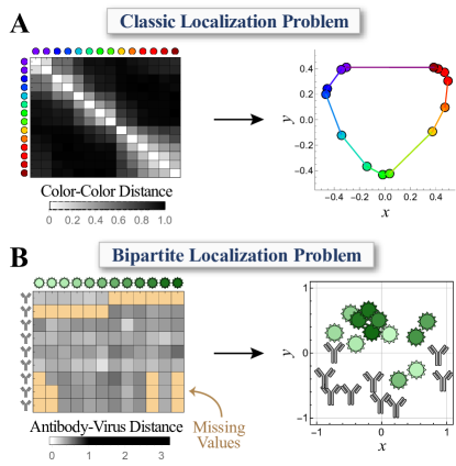
Figure 1: Embedding monopartite or bipartite data in Euclidean space. (A) The perceived similarity between colors recovers the canonical color wheel. Adapted from Table 4.1 of [26], with distance=1-(dissimilarities in table). (B) Embedding antibody neutralization against strains of the influenza virus. In this case, only antibody-virus distance can be measured experimentally, and some distances are missing (tan). Viruses are colored from lightest-to-darkest hues (oldest to more recent strains; full data in Figure S1). Adapted from Figure 5 of [27], with distance=$\log_{10}(\frac{\text{50\% Neutralization}}{10^{-10}\text{Molar}})$.

The Need for Embedding Algorithms

Before exploring the algorithms, we motivate the need for such embeddings by describing several potential applications. To ground this discussion, we suppose the bipartite classes represent antibodies and viruses (with distances describing antibody-virus interactions), although these applications generalize to any bipartite dataset.

First, an embedding combines datasets and predicts unmeasured interactions. For example, we cannot directly compare an antibody measured against viruses #1-6 with a second antibody measured against viruses #7-12 (top two rows in the Figure 1B dataset). Yet by embedding both antibodies, we predict their behavior against all viruses in the dataset. Hence, embeddings represent a form of matrix completion [28, 29].

Second, an embedding defines the intra-class distances between any two viruses (or two antibodies), a quantity that by definition cannot be directly measured through antibody-virus interactions. This intra-class distance describes how differently any antibody can neutralize the two viruses (i.e., essentially quantifying their cross-reactivity). In the limit where two viruses lie on the same point, they will be neutralized identically by all antibodies; when the two viruses lie far apart, their neutralization can greatly differ.

Third, the inferred virus-virus distances are crucial when designing future experiments. Viruses that are close together offer redundant information, whereas sampling viruses that are spread out across the map can detect more distinct antibody phenotypes.

Fourth, an embedding defines a basis set of behaviors, which is essential for systems where no mechanistic models exist. For example, there is a dearth of models that enumerate the space of antibody behaviors [30, 31, 32], which hinders theoretical exploration into features such as the optimality or degeneracy of the antibody response (both of which we address later in this work).

Finally, embeddings provide a fundamentally different vantage to study a system, and this shift in perspective could help uncover its underlying rules. For example, the complex sequence-to-function relationship of viral proteins may be simpler to crack within a low-dimensional embedding. Similarly, the antibody response changes with each viral exposure, and the dynamics of how each antibody evolves may be more readily understood within the context of an embedding.

Algorithms

We next develop the algorithms to transform pairwise interactions into a global map of a system. In bipartite embedding, we seek to recover the bipartite set of points $\{x_{i}^{*}\}_{i=1}^{m},\{y_{j}^{*}\}_{j=1}^{n}\subset\mathbb{R}^{d}$ given the noisy distance matrix $D\in\mathbb{R}^{m\times n}$ of the form

$$D_{ij}=D_{ij}^{*}+\epsilon_{ij},\,\,\,D_{ij}^{*}=\|x_{i}^{*}-y_{j}^{*}\|,$$ (1)

where distance is only measured between the $\{x_{i}^{*}\}$ and $\{y_{j}^{*}\}$. $D_{ij}^{*}$ represents the true distance that is perturbed with independently and identically distributed random noise $\epsilon_{ij}$. The goal is to use the noisy $D_{ij}$ with $(i,j)\in\mathcal{E}$, where $\mathcal{E}$ represents the subset of measured values, to find an embedding $\{x_{i}\}_{i=1}^{m},\{y_{j}\}_{j=1}^{n}$ that approximates the true embedding $\{x_{i}^{*}\},\{y_{j}^{*}\}$. In the following sections, we describe three algorithms to tackle this problem.

Metric Multidimensional Scaling (Metric MDS)

The straightforward numerical approach is to randomly initialize each $x_{i}$ and $y_{j}$, and then apply numerical methods (e.g., gradient descent or differential evolution) to match their coordinates as closely as possible to the distance matrix. In this paper, we use the least-squares loss function

$$\min_{\{x_{i}\}^{m}_{i=1},\{y_{j}\}^{n}_{j=1}}\sum_{(i,j)\in\mathcal{E}}(D_{ij}-\lVert x_{i}-y_{j}\rVert)^{2},$$ (2)

although we note that other loss functions can strongly affect the embedding (Figure S2). While this method is simple to implement, it is liable to get trapped in local minima and does not harness the underlying structure of the bipartite data.

Bipartite Multidimensional Scaling (Bipartite MDS)

In stark contrast, bipartite MDS provides a closed-form solution (up to a rigid transform) for noise-free and complete data. Although variants of the classical monopartite problem have been developed to deal with large datasets and noisy measurements [33], to our knowledge this technique has not been extended to complete bipartite data.

The key insight underlying classic MDS is that the doubly-centered squared-distance matrix is intimately related to the inner products (Gram matrix) of the embedded points. More precisely, we define the centering matrix that subtracts the mean from any vector,

$$J_{k}=I_{k}-\frac{1}{k}\textbf{1}_{k}\textbf{1}_{k}^{T}\in\mathbb{R}^{k\times k},$$ (3)

where $I_{k}$ is the $k\times k$ identity matrix and $\textbf{1}_{k}$ is the all-ones vector of size $k$ (with $J_{k}\mathbf{1}_{k}=\mathbf{0}$). Consider the complete noise-free bipartite graph,

$$(D^{*}\circ D^{*})_{ij}={D^{*}_{ij}}^{2}=\|x_{i}^{*}\|^{2}+\|y_{j}^{*}\|^{2}-2(x_{i}^{*})^{T}y_{j}^{*},$$ (4)

where $\circ$ denotes entrywise multiplication. Double-centering reveals the inner products of the embedding $X^{*}=[x_{1}^{*},\ldots,x_{m}^{*}]^{T}\in\mathbb{R}^{m\times d}$ and $Y^{*}=[y_{1}^{*},\ldots,y_{n}^{*}]^{T}\in\mathbb{R}^{n\times d}$ (Appendix A.4),

$$-\frac{1}{2}J_{m}(D^{*}\circ D^{*})J_{n}=J_{m}X^{*}(Y^{*})^{T}J_{n}=X^{*}(Y^{*})^{T}J_{n},$$ (5)

where in the second equality we assume without loss of generality that the points in $X^{*}$ are centered at the origin ($J_{m}X^{*}=X^{*}$).

The rank $d$ singular value decomposition (SVD) of the double-centered squared-distance matrix, $U\Sigma V^{T}=-\frac{1}{2}J_{m}(D^{*}\circ D^{*})J_{n}$, determines the embedding of $X^{*}$ and $Y^{*}$ up to linear transforms,

$$X^{*} =U\Sigma A_{U}$$ (6)

$$Y^{*} =VA_{V}+\textbf{1}(t_{V})^{T},$$ (7)

for some matrices $A_{U},A_{V}\in\mathbb{R}^{d\times d}$ (satisfying $A_{U}A_{V}^{T}=I_{d}$) and a translation $t_{V}\in\mathbb{R}^{d}$ between the centers of $X^{*}$ and $Y^{*}$. Lastly, $A_{V}$ and $t_{V}$ (together with $A_{U}=(A_{V}^{T})^{-1}$) are determined by utilizing the distance information $\lVert x_{i}^{*}-y_{j}^{*}\rVert=D_{ij}^{*}$ and minimizing (2) using semidefinite programming or numeric minimization (Appendix A.4).

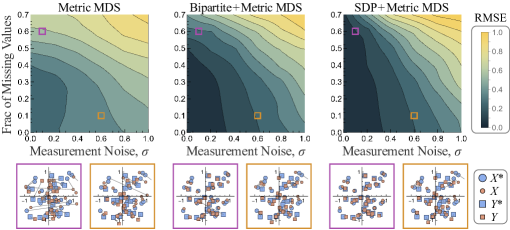
Figure S3: Post-processing an embedding with metric MDS. As in Figure 2, data is simulated with element-wise noise $\sigma$ and a fraction $f_{\text{Missing}}$ of missing entries. The results of each embedding is used to initialize one additional metric MDS, which greatly improves its accuracy. Error is computed as the average Euclidean distance between the numerical and actual coordinates (aligned using a rigid transform). Example plots at the bottom show an embedding when $\sigma=0.1$ and $f_{\text{Missing}}=0.6$ (purple box) as well as $\sigma=0.6$ and $f_{\text{Missing}}=0.1$ (brown box) for each method.

In summary, this algorithm reduces the embedding problem with $(m+n)d$ unknown variables into the simpler problem of determining the $d^{2}+d$ unknown variables in $A_{V}$ and $t_{V}$, regardless of the size of $D$! This same approach can be used for a noisy distance matrix $D$ (Algorithm 1). A caveat of this method is that it cannot readily handle missing values. In the numerical experiments below, we first fill in any missing values using the mean of all observed entries in the same row and column of the distance matrix – this leads to poor behavior when a substantial fraction of values are missing, which can be ameliorated with metric MDS post-processing (Figure S3).

Algorithm 1 Classical Multidimensional Scaling (Bipartite MDS)

Input:

• Distance matrix $D\in\mathbb{R}^{m\times n}$

• Dimension $d$ of the embedding

Steps:

1. Define a complete distance matrix $\tilde{D}$ equal to $D$ at measured values, with missing values filled in using the mean of all observed entries in the same row and column

2. Compute the double-centered matrix, $Q=-\frac{1}{2}J_{m}(\tilde{D}\circ\tilde{D})J_{n}$

3. Compute the top $d$ SVD, $Q=U\Sigma V^{T}$

4. Set $\{x_{i}\}_{i=1}^{m}=U\Sigma A_{U}$ and $\{y_{j}\}_{j=1}^{n}=VA_{V}+\textbf{1}(t_{V})^{T}$ for linear transforms $A_{U},A_{V}\in\mathbb{R}^{d\times d}$ and translation vector $t_{V}\in\mathbb{R}^{d\times 1}$ (where $A_{U}A_{V}^{T}=I$). Determine $A_{U}$, $A_{V}$, and $t_{V}$ by minimizing the difference between ${D}_{ij}$ and $\lVert x_{i}-y_{j}\rVert$ using non-convex numerical minimization or SDP (see Appendix A.4)

Semidefinite Programming (SDP)

Lastly, we investigate an intermediate algorithm that harnesses the bipartite nature of the data to perform a more robust numerical search. More precisely, by forming a positive-semidefinite matrix, we can adapt the sensor network localization SDP algorithm [6] and utilize efficient conic solvers for bipartite embedding [34, 35]. We define the combined coordinates $Z=\begin{pmatrix}X\\ Y\end{pmatrix}\in\mathbb{R}^{(m+n)\times d}$ where $X,Y$ store $\{x_{i}\}_{i=1}^{m},\{y_{j}\}_{j=1}^{n}$. We further define the inner product matrix $G\in\mathbb{R}^{(m+n)\times(m+n)}$ as

$$Z{Z}^{T}=\begin{pmatrix}X{X}^{T}&X{Y}^{T}\\ Y{X}^{T}&Y{Y}^{T}\end{pmatrix}\equiv\begin{pmatrix}G_{11}&G_{12}\\ G_{12}^{T}&G_{22}\end{pmatrix}\equiv G,$$ (8)

so that the squared-distance between $x_{i}$ and $y_{j}$ can be entirely written in terms of the entries of $G$, namely,

$$\|x_{i}-y_{j}\|_{2}^{2}=(G_{11})_{ii}-2(G_{12})_{ij}+(G_{22})_{jj}.$$ (9)

Note that we can exactly recast the optimization over $X$ and $Y$ in terms of an optimization over a positive semidefinite matrix $G$ of rank $d$. The goal is then to minimize $\sum_{(i,j)\in\mathcal{E}}|(G_{11})_{ii}-2(G_{12})_{ij}+(G_{22})_{jj}-D_{ij}^{2}|$ in terms of $G$. To this end, we introduce an extra error matrix $E\in\mathbb{R}^{m\times n}$ and minimize over the sum of errors:

$$\begin{matrix}[l]\underset{G,E}{\text{minimize}}&\sum_{(i,j)\in\mathcal{E}}E_{ij}\\ \text{subject to}&E\geq 0,G\succeq 0,\\ &-E_{ij}\leq(G_{11})_{ii}-2(G_{12})_{ij}+(G_{22})_{jj}-D_{ij}^{2}\leq E_{ij},\quad(i,j)\in\mathcal{E}\\ &\sum_{j=1}^{n}G_{ij}=0,\,\,\,\,\forall 1\leq j\leq m.\end{matrix}$$ (10)

The final constraint ensures that the $X$ coordinates are centered at the origin, removing their translational degree of freedom. Note that to achieve this convex conic program, we removed the non-convex $\text{rank}(d)$ constraint of $G$, which must now be added back. Thus, we apply an SVD to $G$ of rank $d$, $G=U\Sigma V^{T}$. The resulting $m+n$ coordinates are given by $\begin{pmatrix}X\\ Y\end{pmatrix}=U\sqrt{\Sigma}$ (Algorithm 2).

As with metric MDS, missing values are seamlessly handled in SDP since the objective in Equation 10 is restricted to the measured distances. As shown in the following sections, SDP often recovers a better embedding than metric or bipartite MDS, especially when there are many missing values. Note that we specifically chose a different loss function for metric MDS (Equation 2, optimized for systematic noise) and SDP ($\sum_{(i,j)\in\mathcal{E}}\lvert\lVert x_{i}-y_{j}\rVert^{2}-D_{ij}^{2}\rvert$, optimized to handle outliers) in order to explore the diversity of embedding behaviors. When analyzing datasets, it is worth trying multiple loss functions to determine which one best characterizes the system (Figure S2C). For completeness, we note that bipartite MDS is a closed-form method that does not explicitly use any loss function.

Algorithm 2 Semidefinite Programming (SDP)

Input:

• Distance matrix $D\in\mathbb{R}^{m\times n}$

• Dimension $d$ of embedding

Steps:

1. Solve $G\in\mathbb{R}^{(m+n)\times(m+n)}$ from Equation 10

2. Compute the top $d$ SVD, $G=U\Sigma U^{T}$. The embedded coordinates $\{x_{i}\}$ are given by the first $m$ rows of $U\Sigma^{1/2}$ while $\{y_{j}\}$ are given by the final $n$ rows

Numerical Experiments

We first assess the three embedding algorithms – metric MDS , bipartite MDS, and SDP – using simulated data with $m=20$ entries $x_{i}$ and $n=20$ entries $y_{j}$ (each chosen uniformly on $[-1,1]\times[-1,1]$). These points generate the true distance matrix, which we then perturb and use as the input matrix $D$. The accuracy of the resulting embedding is calculated using the RMSE of Euclidean distances, $\sqrt{(\sum_{i=1}^{m}\|x_{i}-x_{i}^{*}\|^{2}+\sum_{j=1}^{n}\|y_{j}-y_{j}^{*}\|^{2})/(m+n)}$, between the estimated and true coordinates (once aligned via a rigid transform).

Systematic Noise and Missing Values

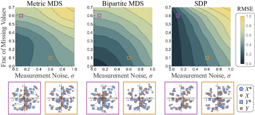
Figure 2: Performance on a simulated dataset. Top, Phase diagram of embedding error as a function of the element-wise noise $\sigma$ of the distance matrix and the fraction $f_{\text{Missing}}$ of missing entries for metric multidimensional scaling (metric MDS), bipartite multidimensional scaling, and semidefinite programming (SDP). Error is computed as the average Euclidean distance between the numerical and true coordinates (aligned using a rigid transform). Diagrams show the average of 10 runs, and the metric MDS results were smoothed because its embedding accuracy was erratic. Bottom, Examples of the embedding when $\sigma=0.1$ and $f_{\text{Missing}}=0.6$ (purple box) as well as $\sigma=0.6$ and $f_{\text{Missing}}=0.1$ (brown box) for each method. Edges connect the numerical coordinates to the true embedding.

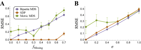
Figure S4: Embedding for noise-free or complete datasets. (A) The noise-free limit $\sigma=0$ and (B) the limit of complete data $f_{\text{Missing}}=0$. In both panels, $m=n=20$ and the error represents the RMSE of Euclidean distances between the the estimated and true coordinates (once aligned via a rigid transform).

To generate the input matrix $D$, we perturb each entry of the true distance matrix by adding a random value uniformly chosen from $[-\sigma,\sigma]$ ($x$-axis) and withhold a fraction $f_{\text{Missing}}$ of randomly selected entries ($y$-axis). Of the three algorithms, SDP exhibits the most robust behavior in the presence of missing values (Figure 2), and in the noise-free case along the $y$-axis it undergoes a phase transition from near-perfect recovery when $f_{\text{Missing}}\leq 0.6$ to noisy recovery (Figure S4A). In contrast, the error of bipartite MDS increases nearly proportionally to $f_{\text{Missing}}$, since each missing value must be initialized as the row/column mean which effectively perturbs the distance matrix. Metric MDS also finds poorer embeddings with larger $f_{\text{Missing}}$, as it occasionally gets trapped in local minima (even in the low-noise limit).

When $D$ is fully observed along the $x$-axis, the error increases approximately linearly with noise for all three algorithms ($\text{RMSE}\approx\sigma/2$, Figure S4B), although metric MDS displays somewhat erratic behavior as it may get stuck in local minima. The bottom panels in Figure 2 show example embeddings in the intermediate regimes when $\sigma=0.1$ and $f_{\text{Missing}}=0.6$ (purple) or when $\sigma=0.6$ and $f_{\text{Missing}}=0.1$ (brown), with gray lines connecting the true coordinates to their numerical approximations.

In terms of overall performance, the region of near-perfect recovery is largest for SDP followed by bipartite MDS and metric MDS (Figure 2). One way to improve these algorithms is to combine them, for example, by using SDP or bipartite MDS to initialize the coordinates in metric MDS. These combined algorithms substantially improve embedding accuracy, allowing bipartite MDS to handle missing values and extending the capability of SDP to embed noisy measurements (Figure S3).

Handling Large Outliers and Bounded Measurements

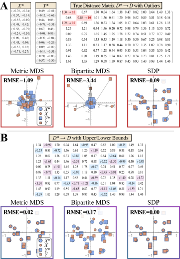
Figure 3: Embedding with outliers and bounded data. (A) Embedding a noise-free distance matrix $D$ with three highly-corrupted measurements (highlighted in red). (B) Embedding a distance matrix where 30% of entries are replaced with upper or lower bounds (blue and purple).

In addition to noisy measurements, datasets may contain outliers that distort an embedding. Bipartite MDS is highly susceptible to large outliers, which can corrupt the largest singular vectors of the squared-distance matrix (Figure 3A). In contrast, SDP minimizes the sum of absolute (un-squared) deviation [36], and such loss is far more robust against gross corruptions. Metric MDS exhibits intermediate behavior, although we note that the choice of loss function heavily influences this behavior (Figure S2).

Lastly, we explored each algorithm’s tolerance to distances given as upper or lower bounds, which can arise when an experiment measures a value outside of its dynamic range. Figure 3B shows the embedding from the same distance matrix, now modified to represent 30% of measurements as upper or lower bounds. In this complete and noise-free case, both metric MDS and SDP can directly utilize these bounds to generate near-perfect reconstructions. In contrast, bipartite MDS cannot directly incorporate bounded data, and hence we replace each bounded measurement by the bound itself, which leads to worse reconstruction.

Analysis of Antibody-Virus Measurements

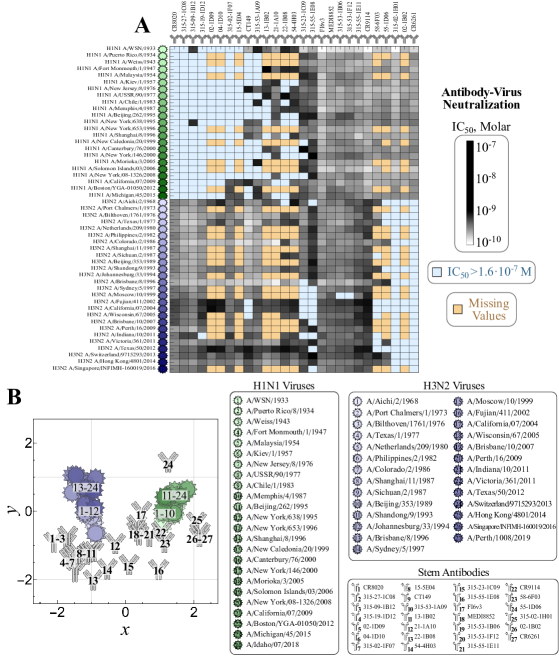
Figure S1: Annotated influenza antibody-virus data from Creanga et al. [27]. (A) Neutralization measurements of 49 influenza viruses against 27 antibodies targeting the stem of influenza hemagglutinin. The inhibitory concentration of antibody needed to neutralize 50% of viruses ($\text{IC}_{50}$, grayscale). Some antibody-virus interactions were not measured (tan), and some antibodies exhibited weak neutralization ($\text{IC}_{50}>1.6\cdot 10^{-7}\,\text{M}$, light-blue) outside the dynamic range of the assay. (B) The same 2D metric MDS embedding (as in Figure 4B) with the antibodies and viruses labeled.

We next applied these embedding algorithms to an influenza dataset where the neutralization from 27 stem antibodies was measured against 49 viruses that circulated between 1933-2019 (Figure S1). The following section transforms these experimental measurements into map distances to embed these antibody-virus interactions, while all subsequent sections utilize this embedding to probe the antibody response.

Transforming Antibody-Virus Measurements into Distances

For each antibody-virus pair, the inhibitory concentration required to neutralize 50% of virus particles ($\text{IC}_{50}$ in Molar units) was measured, with lower values signifying a more potent antibody [27]. $\text{IC}_{50}$s ranged from $8.6\cdot 10^{-11}\,\text{M}$ (very strong neutralization) to $>$$1.6\cdot 10^{-7}\,\text{M}$ (weak neutralization outside the range of the assay).

To briefly describe the biological context for this dataset, each of the 27 antibodies targets the stem region of hemagglutinin, one of the key surface proteins on the influenza virus. This stem domain is highly conserved, and antibodies targeting it can neutralize very diverse viruses; for example, some antibodies measurably neutralize both the H1N1 and H3N2 influenza subtypes, which is rarely seen in antibodies targeting the head domain of this same viral protein [37].

Yet even these broadly neutralizing antibodies have limits. Antibodies that potently neutralize H1N1 viruses tend to weakly neutralize H3N2 strains (and vice versa), while antibodies that neutralize all viruses tend to have intermediate effectiveness. These trends hint that there is an underlying tradeoff between antibody potency (how much a virus is neutralized) and breadth (how many diverse viruses can be neutralized). Such patterns are difficult to directly discern from a table of pairwise interactions, yet they naturally emerge through an embedding.

To that end, we first converted these antibody-virus neutralization measurements into distances. Antibodies typically have $\text{IC}_{50}$s$\,>10^{-10}\,\text{M}$ (since selection does not act below this point [38, 39]), and hence we define antibody-virus distance as $D_{ij}=\log_{10}\left(\frac{\text{IC}_{50}}{10^{-10}\,\text{M}}\right)$ (Figure 4A). We then applied all three embedding algorithms to create a global map of the system. Since both the dimensionality and the ground truth coordinates are not known, we assessed each algorithm through cross validation (training on 90% of data, testing on the remaining 10%).

Metric MDS performed the best in all dimensions and exhibited a sharp “elbow” at $d=2$, suggesting that a 2D landscape captures the underlying structure of the system (Figure 4C). We note that the 2D cross-validation RMSE was 0.44 (Figure 4D), so that withheld neutralization measurements are predicted within $10^{0.44}\approx 3$-fold, which is comparable to the noise of the neutralization assay.

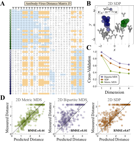
Figure 4: Mapping influenza antibody-virus interactions. (A) Experimentally measured distance matrix between 27 antibodies and 49 influenza viruses [27]. (B) The metric MDS embedding in 2D. (C) 10-fold cross validation RMSE (calculated using the distance matrix). (D) Example of 2D cross validation for each method, demonstrating that metric MDS performs the best.

Designing Optimal Antibody Cocktails

The resulting map provides a powerful way to quantify trends in the data (Figure 4B). For example, the H1N1 viruses [green] and H3N2 viruses [blue] cluster together, as expected based on their genetic similarity. Interestingly, the centers of these clusters are $\approx\,$2.5 map units apart, demonstrating that while antibodies can be highly potent against H1N1 or H3N2 viruses, no antibody in the panel could strongly neutralize both subtypes.

Similar to the color wheel example in Figure 1A, the antibody-virus embedding not only represents the entities in this specific dataset, but also describes other potential antibodies and viruses. For such entities, the embedding serves as a discovery space to quantify and constrain their behavior.

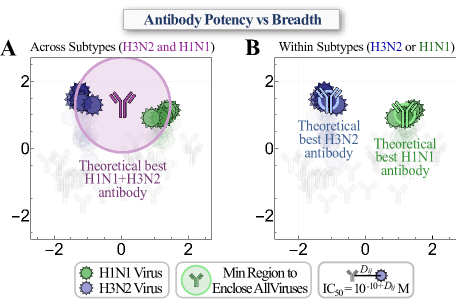
Figure S5: Predicting optimal neutralization for any mapped viruses. Suppose we want to neutralize the five viruses at the tops of the H1N1 and H3N2 clusters in Figure 4B (H1N1 A/New York/638/1995, A/Beijing/262/1995, H1N1 A/New Caledonia/20/1999, A/Canterbury/76/2000, A/New York/146/2000 and H3N2 A/Fujian/411/2002, A/California/07/2004, A/Indiana/10/2011, A/Texas/50/2012, A/Perth/1008/2019). Using the points on the map to represent potential antibody neutralization profiles, we determine (A) the best single antibody or (B) the best 2-antibody mixture that would neutralize these viruses the most potently (with the smallest possible distance between any virus and the nearest antibody). The solution is given by the $n$ minimum covering circles for these viruses, with the antibodies positioned at the centers of each circle.

For example, within this framework we can design a mixture of $n$ antibodies that optimally neutralizes the 5 viruses at the top of the H1N1 cluster as well as the 5 viruses at the top of the H3N2 cluster as potently as possible (Figure S5). This question lies at the heart of ongoing efforts to find new broadly-neutralizing antibodies, yet few methods exist to predict or even constrain antibody behavior. To that end, we use each point on the map to describe a potential antibody whose neutralization against each mapped virus is determined by its map-distance. This reduces the complex biological problem of enumerating antibody behavior to a straightforward geometry problem.

The best $n=1$ antibody mixture against these 10 viruses is represented by the center of the smallest circle that covers every virus (Figure S5, $\text{distance}\!\leq\!1.4$ [$\text{IC}_{50}\!\leq\!10^{-8.6}\,\text{M}$] for each virus). For a mixture with $n=2$ antibodies, the potency dramatically improves by using one H1N1-specific antibody and one H3N2-specific antibody ($\text{distance}\!\leq\!0.3$ [$\text{IC}_{50}\!\leq\!10^{-9.7}\,\text{M}$] for each virus). This problem can be readily extended to mixtures with an arbitrary $n$ antibodies covering any set of mapped viruses. Given the growing number of efforts to find broadly neutralizing antibodies [40, 41, 42, 43], it is essential to have some framework to estimate the limits of antibody behavior. Such estimations inform when the antibodies already discovered are near the theoretical best behavior (and hence further searching is less likely to lead to significant improvement) or when there are alleged antibodies that could perform orders of magnitude better than what we have currently seen [44].

Degeneracy of the Antibody Response

Another key unexplored feature of the antibody response is its degeneracy: can the neutralization from a mixture of $n$ antibodies behave like a mixture with fewer antibodies? For example, many vaccination regiments aim to elicit a broadly-neutralizing antibody that will be potent against diverse viral strains. Yet even if a post-vaccination antibody response is measured against a large array of viruses, it may be impossible to determine whether its breadth is conferred by a single antibody or due to the collective action of multiple antibodies. These questions hint at an underlying gap in our knowledge, namely, quantifying when antibody mixtures “unlock” fundamentally new behaviors that cannot be achieved by any individual antibody. Moreover, these topics are difficult to tackle experimentally, since the low-throughput neutralization assay is time- and resource-intensive.

Nevertheless, quantifying the degree of antibody degeneracy becomes tractable through an embedding. Such analyses necessarily make the strong assumption that every point on the map represents a viable antibody. Moreover, there may be other antibody phenotypes (e.g., from highly-specific hemagglutinin head-targeting antibodies) that are not represented by any point on the map; in essence, the embedding serves to locally extrapolate antibody behavior based on the specific interactions provided as input (Figure 4A). Yet with these caveats, we can explore how often a mixture made within this space of antibodies can be mimicked by a single antibody.

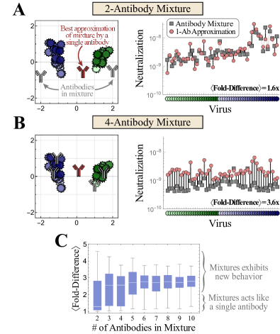
Figure 5: Degeneracy of antibody mixtures. Examples of (A) a 2-antibody mixture that behaves like a single antibody and (B) a 4-antibody mixture that exhibits distinct behavior from any individual antibody. Left, the antibodies in the mixture (gray) and the best approximating antibody (red). Right, the neutralization $\text{IC}_{50}$s across all viruses. The fold-difference between the mixture and antibody is shown by the vertical black lines for each virus, with the mean fold-difference given in the bottom-right. (C) For each mixture containing $n$ antibodies ($x$-axis), we sample 100 equimolar mixtures and quantify their average fold-difference to the nearest approximating antibody.

We describe an antibody mixture by $n$ points in Figure 4B, with the $i^{\text{th}}$ antibody neutralizing the $j^{\text{th}}$ virus with an $\text{IC}_{50}^{ij}=10^{-10+D_{ij}}$ dictated by the map distance $D_{ij}$ between the antibody and virus. Since all antibodies in our panel bind to the same region of the hemagglutinin stem [45, 46, 47], we treat their binding as competitive, so only one antibody can bind to each hemagglutinin monomer at a time. Thus, a mixture’s neutralization against virus $j$ is given by

$$\text{IC}_{50}^{\text{Mixture}}=\left(\sum_{i}\frac{f_{i}}{\text{IC}_{50}^{ij}}\right)^{-1}$$ (11)

where $f_{i}$ represents the fraction of antibody $i$ in the mixture (with $\sum_{i}f_{i}=1$). A diluted antibody with small $f_{i}$ will effectively have a weaker (larger) $\text{IC}_{50}$, which in the embedding translates to an extra “distance handicap” of $\log_{10}f_{i}$ added to its distance from any virus. We note that this binding model has been verified on antibody mixtures from this specific panel [44] and on other datasets [48, 49]. For simplicity, we restrict ourselves to equimolar $n$-antibody mixtures ($f_{i}=1/n$).

Given a specific mixture ($n$ random points on the map, sampled near the H1N1 and H3N2 clusters), we quantify the closest approximating single antibody (another point on the map) by scanning through every possible location and minimizing the average fold-difference between the mixture’s and antibody’s neutralization profiles across all viruses. Figure 5A shows a mixture of 2-antibodies (gray), one of which is potent against the blue H3N2 viruses on the left of the map and the other potent against the green H1N1 viruses, that behave nearly identically to a single antibody (red) in the middle of the map. While a few viruses are neutralized differently by the mixture and antibody (vertical black lines, right panel of Figure 5A), on average the antibody’s $\text{IC}_{50}$s are within 1.6-fold of the mixture’s values against these 50 diverse viruses. This discrepancy is comparable to the $\approx$2-fold error of the assay, and hence given either neutralization profile, we could not determine whether it arose from an individual antibody or a mixture.

Higher-order mixtures unlock more unique behaviors that cannot be replicated by an individual antibody. For example, not only does the 4-antibody mixture in Figure 5B show a 3.6-fold difference from the nearest approximating antibody, but the mixture’s measurements are systematically lower across nearly all viruses. Thus, neutralization profiles exhibiting such strong breath are indicative of multiple antibodies.

To systematically explore degeneracy, we sampled 100 antibody mixtures for each $n$ (with $2\leq n\leq 10$) and found the closest approximating single antibody. The resulting distributions of the mean fold-difference are shown in Figure 5C. While 2-antibody mixtures tend to resemble individual antibodies, higher order mixtures often exhibit distinctive profiles with a $\langle\text{fold-difference}\rangle>2$ to the closest approximating antibody. By the time $n\geq 5$ antibodies are combined, the likelihood that they match any single antibody becomes exceedingly rare.

Discussion

Embedding algorithms fill a “hole” in our understanding by transforming local pairwise interactions into a global map. Such algorithms have been used to identify when a new viral variant arises, quantify drug-protein interactions, and distinguish between cell types [25, 50, 51]. Yet we propose that such algorithms also provide the groundwork for new theoretical studies that only become possible when we reveal the underlying structure of a system.

In the context of antibody-virus interactions, an embedding provides a rigorous approach to extrapolate available measurements. Each point describes a potential antibody, and the entire map defines a basis set of antibody behaviors. By coupling these data-driven results with a biophysical model of how antibodies collectively act, we can model higher-order mixtures and pave the way to study the complex array of antibodies within each person.

More work is needed to understand the limits of these embeddings and quantify their predictive power. At the same time, we are just beginning to scratch the surface on aspects of the antibody response that can be probed with these embeddings, from designing antibody cocktails to determining how the antibody response evolves on the map with each viral exposure.

As datasets continue to grow in size and complexity, it becomes increasingly important to quantitatively visualize interactions between entities. Future datasets may require multi-localization, where higher-order interactions (e.g., between a ligand and multimeric receptor [22]; antibodies, antigens, and cell receptors [52]; or single-cell multi-omics datasets [53]) are embedded in a low-dimensional space.

Appendix A Supplemental Methods

The sections below describe the implementations of metric MDS, bipartite MDS, and SDP algorithms. Complete Mathematica code is available on GitHub (https://github.com/TalEinav/Bilocalization).

A.1 Solving the classical localization problem for complete, noise-free data

Here, we present the well-known solution to the (monopartite) classical localization problem, where the noise-free distances $D\in\mathbb{R}^{n\times n}$ is provided between every pair of $n$ points in $d$ dimensions. Our goal is to determine the coordinates $\{x_{i}\}_{i=1}^{n}\subset\mathbb{R}^{d}$ such that $D_{ij}=\lVert x_{i}-x_{j}\rVert$.

Since an embedding always has a translational degree of freedom, we will assume without loss of generality that the coordinates are centered around the origin, $\sum_{i=1}^{n}x_{i}=\mathbf{0}$. We define the combined coordinate matrix $X=[x_{1},\ldots,x_{n}]^{T}\in\mathbb{R}^{n\times d}$. Note that the entrywise squared-distance matrix can be written as

$$D\circ D=\text{diag}(XX^{T})\mathbf{1}_{n}^{T}+\mathbf{1}_{n}\text{diag}(XX^{T})^{T}-2XX^{T}$$ (S1)

where the first two terms on the right-hand side are outer products.

The algorithm proceeds in two steps. First, we apply the centering matrix $J_{n}$ (Equation 3) from the left and right to row-center and column-center the squared-distances,

$$-\frac{1}{2}J_{n}(D\circ D)J_{n}=XX^{T},$$ (S2)

where we used the fact that $J_{n}\mathbf{1}_{n}=\mathbf{0}$ and $\mathbf{1}_{n}^{T}J_{n}=\mathbf{0}$. This transforms the distance matrix into a matrix of inner products for the coordinates, $XX^{T}$.

The second step is to compute the SVD of the left-hand side, $U\Sigma U^{T}=XX^{T}$, which will only have $d$ non-zero singular values. From this form, we can immediately read out the solution $X=U\Sigma^{1/2}$.

A.2 Handling missing values in the distance matrix

In metric MDS and SDP, missing values are automatically ignored, since the sums in 2 and 10 are over the measured distances, $(i,j)\in\mathcal{E}$. In other words, each measured edge constrains the embedding while unmeasured edges are ignored. Bipartite MDS requires a complete matrix to compute the SVD, and hence each missing entry is first filled in using the mean of all non-missing measurements in its row and column.

A.3 Handling upper or lower bounds in the distance matrix

Sometimes measurements are given as upper or lower bounds on $\|x_{i}-y_{j}\|$ (signifying weak or strong interactions outside the dynamic range of the experiment).

For an upper bound $\lVert x_{i}-y_{j}\rVert<b_{\text{up}}$ in metric MDS, we modify the relevant summand in the loss function to $\frac{1}{1+e^{c(b_{\text{high}}-\lVert x_{i}-y_{j}\rVert)}}\left(b_{\text{high}}-\lVert x_{i}-y_{j}\rVert\right)^{2}$ where $c>0$ is a positive constant (in this work, we chose $c=10$ based on the scale of the distance measurements). The prefactor in the summand penalizes violations of the bound while minimally increasing the loss when the bound is satisfied. For a lower bound, $\lVert x_{i}-y_{j}\rVert>b_{\text{low}}$, we similarly modify the summand to $\frac{1}{1+e^{-c(b_{\text{low}}-\lVert x_{i}-y_{j}\rVert)}}\left(b_{\text{low}}-\lVert x_{i}-y_{j}\rVert\right)^{2}$. Note that the resulting cost function is non-convex, which can prevent numerical algorithms from finding a good minimizer. When computing RMSE in the cross-validation analysis (Figure 4C,D), we added these same prefactors when the measured distance was an upper or lower bound.

Bipartite MDS requires exact distance measurements to compute an SVD, and hence we replace each bounded measurement by the bound itself, which leads to poorer embeddings.

In SDP, bounded values are handled by modifying the second constraint in Problem 10. For example, an upper bound $\|x_{i}-y_{j}\|<b_{\text{up}}$ is enforced by the one-sided constraint $(G_{11})_{ii}-2(G_{12})_{ij}+(G_{22})_{jj}-b_{\text{up}}^{2}<E_{ij}$. A lower bound $\|x_{i}-y_{j}\|>b_{\text{low}}$ is enforced by the one-sided constraint $-E_{ij}<(G_{11})_{ii}-2(G_{12})_{ij}+(G_{22})_{jj}-b_{\text{low}}^{2}$. The objective remains the same, namely, to minimize the sum of (positive) errors $E_{ij}$ between the embedding and distance measurements.

A.4 Determining the affine transformation in Bipartite MDS

In this section, we provide some intuition for bipartite MDS and describe in detail the final SDP step that determines the affine transform between $X$ and $Y$.

We begin by rewriting Equation (4) as

$${D^{*}}\circ D^{*}=\text{diag}(X^{*}{X^{*}}^{T})\mathbf{1}_{n}^{T}+\mathbf{1}_{m}\text{diag}(Y^{*}{Y^{*}}^{T})^{T}-2{X^{*}}^{T}Y^{*}.$$ (S3)

Because $\mathbf{1}_{m},\mathbf{1}_{n}$ lie in the nullspace of $J_{m},J_{n}$, double-centering isolates the inner product term as in Equation (5). Using the rank-$d$ SVD $U\Sigma V^{T}=-\frac{1}{2}J_{m}(D^{*}\circ D^{*})J_{n}$, we can rewrite Equation (5) as

$$X^{*}=U\Sigma(V^{T}({Y^{*}}^{T}J_{n})^{\dagger}),\quad J_{n}Y^{*}=V(\Sigma U^{T}({X^{*}}^{T})^{\dagger}).$$ (S4)

where “$\dagger$” denotes the pseudo-inverse. This reveals that the embedding $X^{*},Y^{*}$ can be determined up to linear transforms as in Equation (6)-(7).

As described in the main text, the final step of bipartite MDS is to determine the affine transforms $A_{U},A_{V}$ (satisfying $A_{U}A_{V}^{T}=I_{d}$) and the translation $t_{V}$ so that the embeddings $X^{*},Y^{*}$ in Equation (6)-(7) match the distance matrix. This can be done numerically by either minimizing the loss function in Equation (2) that optimally handles systematic noise, or by minimizing the loss function of squared-distances

$$\min_{\{x_{i}\}^{m}_{i=1},\{y_{j}\}^{n}_{j=1}}\sum_{(i,j)\in\mathcal{E}}\lvert{D}_{ij}^{2}-\lVert x_{i}-y_{j}\rVert^{2}\rvert$$ (S5)

that better handles outliers (Figure S2).

Instead of numeric minimization, we can use semidefinite programming to solve Equation (S5) and prevent the minimization from getting stuck at local minimum (note that with semidefinite programming cannot be used with the loss function in Equation (2)). To that end, we construct the $(2d+1)\times(2d+1)$ Gram matrix

$$\tilde{G}=\begin{pmatrix}-\text{ }A_{U}\text{ }-\\ -\text{ }A_{V}\text{ }-\\ -\,\,\,t_{V}^{T}\,\,\,-\end{pmatrix}\begin{pmatrix}|&|&|\\ A_{U}^{T}&A_{V}^{T}&t_{V}\\ |&|&|\end{pmatrix}$$ (S6)

with which we can express $\lVert x_{i}-y_{j}\rVert^{2}$. Using Equations (6)-(7), we can write

$$\lVert x_{i}-y_{j}\rVert^{2}=U_{i}\Sigma A_{U}A_{U}^{T}\Sigma U_{i}^{T}+V_{j}A_{V}A_{V}^{T}V_{j}^{T}+t_{V}^{T}t_{V}-2V_{j}\Sigma U_{i}-2U_{i}\Sigma A_{U}t_{V}+2V_{j}A_{V}t_{V}$$ (S7)

in terms of the entries of $\tilde{G}$.

Define the minimization matrix $\gamma\in\mathbb{R}^{m\times n}$ with $\gamma_{ij}={D}_{ij}^{2}-\lVert x_{i}-y_{j}\rVert^{2}$. To minimize the absolute value of the $\gamma_{ij}$, we use Schur’s complement condition, defining the auxiliary matrix $\tilde{\gamma}\in\mathbb{R}^{m\times n}$ and using semidefinite programming to solve

$$\begin{matrix}[l]\underset{\tilde{G},\tilde{\gamma}}{\text{minimize}}&\sum_{(i,j)\in\mathcal{E}}\tilde{\gamma}_{ij}\\ \text{subject to}&\tilde{G}\succeq 0,\\ &\begin{pmatrix}\tilde{\gamma}_{ij}&\gamma_{ij}\\ \gamma_{ij}&1\end{pmatrix}\succeq 0,\,\,\,\,\forall 1\leq i\leq m,1\leq j\leq n\\ &\tilde{G}_{d+1:2d,1:d}=I_{d}.\end{matrix}$$ (S8)

We then use Cholesky decomposition extract $A_{U}$ from $\tilde{G}_{1:d,1:d}$ and determine $A_{V}=\tilde{G}_{d+1:2d,d+1:2d}A_{U}$ as well as $t_{V}=\tilde{G}_{2d+1,d+1:2d}A_{U}$. The resulting embedding is given by Equations (6)-(7).

A.5 Numeric Minimization in Metric Multidimensional Scaling

Minimization was performed using the default NMinimize in Mathematica with the default search method (Differential Evolution). This method is time-constrained, so that for large distance matrices (where $n+m\gtrsim 100$), it may yield very poor solutions. Although in this work we only ran this minimization once, multiple initial conditions could be run to report the lowest error achieved.

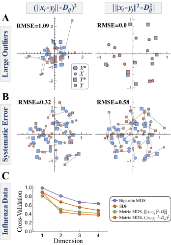
Figure S2: Choice of loss function strongly influences metric MDS. We compare two loss functions for metric MDS: Left column mean squared error between unsquared-distances (shown in the main text) versus right column mean absolute error between the squared-distances. (A) Mean absolute error handles the distance matrix with large outliers far better (see Figure 3A). (B) Large systematic noise is handled better by mean squared error, since this represents the maximum likelihood estimator for approximately-Gaussian error (see $\sigma=1,f_{\text{Missing}}=0$ from Figure 2). (C) Cross-validation for the influenza data in Figure 4 is slightly lower for metric MDS with mean squared error for embeddings with $\text{dimension}\geq 2$.

References

- [1] Joseph B Kruskal “Multidimensional Scaling” Sage, 1978 URL: https://www.google.com/books/edition/Multidimensional˙Scaling/8gpEDwAAQBAJ?hl=en&gbpv=0
- [2] A. Mead “Review of the Development of Multidimensional Scaling Methods” In The Statistician 41.1 JSTOR, 1992, pp. 27 DOI: 10.2307/2348634
- [3] Jan Leeuw and Patrick Mair “Multidimensional Scaling Using Majorization: SMACOF in R” In Journal of Statistical Software 31.3 University of California at Los Angeles, 2009, pp. 1–30 DOI: 10.18637/JSS.V031.I03
- [4] Leo Liberti, Carlile Lavor, Nelson Maculan and Antonio Mucherino “Euclidean Distance Geometry and Applications” In SIAM review 56.1 SIAM, 2014, pp. 3–69 DOI: 10.1137/120875909
- [5] Abdo Y. Alfakih, Amir Khandani and Henry Wolkowicz “Solving Euclidean Distance Matrix Completion Problems Via Semidefinite Programming” In Computational Optimization and Applications 12.1 Springer, 1999, pp. 13–30 DOI: 10.1023/A:1008655427845
- [6] Pratik Biswas, Tzu Chen Liang, Kim Chuan Toh, Yinyu Ye and Ta Chung Wang “Semidefinite programming approaches for sensor network localization with noisy distance measurements” In IEEE Transactions on Automation Science and Engineering 3.4, 2006, pp. 360–371 DOI: 10.1109/TASE.2006.877401
- [7] Kilian Q Weinberger and Lawrence K Saul “An Introduction to Nonlinear Dimensionality Reduction by Maximum Variance Unfolding” In AAAI 2, 2006, pp. 1683–1686 URL: https://dl.acm.org/doi/10.5555/1597348.1597471
- [8] Anthony Man Cho So and Yinyu Ye “Theory of semidefinite programming for Sensor Network Localization” In Mathematical Programming 109.2 Springer, 2006, pp. 367–384 DOI: 10.1007/S10107-006-0040-1
- [9] Kurt Wuthrich “Protein Structure Determination in Solution by NMR Spectroscopy” In Journal of Biological Chemistry 265.36, 1990, pp. 22059–22062 DOI: 10.1016/S0021-9258(18)45665-7
- [10] Bruce R Donald “Algorithms in Structural Molecular Biology” MIT Press, 2011 URL: https://www.google.com/books/edition/Algorithms˙in˙Structural˙Molecular˙Biolo/GSw3AgAAQBAJ?hl=en&gbpv=0
- [11] Amit Singer “A remark on global positioning from local distances” In Proceedings of the National Academy of Sciences 105.28 National Academy of Sciences, 2008, pp. 9507–9511 DOI: 10.1073/PNAS.0709842104
- [12] Robert Connelly and Steven J. Gortler “Universal Rigidity of Complete Bipartite Graphs” In Discrete and Computational Geometry 57.2 Springer, 2017, pp. 281–304 DOI: 10.1007/S00454-016-9836-9
- [13] Ming Gao, Xiangnan He, Leihui Chen, Tingting Liu, Jinglin Zhang and Aoying Zhou “Learning Vertex Representations for Bipartite Networks” In IEEE Transactions on Knowledge and Data Engineering 34.1 IEEE Computer Society, 2022, pp. 379–393 DOI: 10.1109/TKDE.2020.2979980
- [14] Andrey Feuerverger, Yu He and Shashi Khatri “Statistical Significance of the Netflix Challenge” In Project Euclid 27.2 Institute of Mathematical Statistics, 2012, pp. 202–231 DOI: 10.1214/11-STS368
- [15] Xiangnan He, Hanwang Zhang, Min Yen Kan and Tat Seng Chua “Fast matrix factorization for online recommendation with implicit feedback” In SIGIR 2016 Association for Computing Machinery, Inc, 2016, pp. 549–558 DOI: 10.1145/2911451.2911489
- [16] Inderjit S. Dhillon “Co-clustering documents and words using bipartite spectral graph partitioning” In KDD Association for Computing Machinery (ACM), 2001, pp. 269–274 DOI: 10.1145/502512.502550
- [17] Yuval Kluger, Ronen Basri, Joseph T. Chang and Mark Gerstein “Spectral Biclustering of Microarray Data: Coclustering Genes and Conditions” In Genome Research 13.4 Cold Spring Harbor Laboratory Press, 2003, pp. 703 DOI: 10.1101/GR.648603
- [18] Sara C. Madeira and Arlindo L. Oliveira “Biclustering algorithms for biological data analysis: A survey” In IEEE/ACM transactions on computational biology and bioinformatics 1.1, 2004, pp. 24–45 DOI: 10.1109/TCBB.2004.2
- [19] James A. Russell and Merry Bullock “Multidimensional Scaling of Emotional Facial Expressions. Similarity From Preschoolers to Adults” In Journal of Personality and Social Psychology 48.5, 1985, pp. 1290–1298 DOI: 10.1037/0022-3514.48.5.1290
- [20] Eric M Jones et al. “Structural and functional characterization of G protein–coupled receptors with deep mutational scanning” In eLife 9, 2020 DOI: 10.7554/eLife.54895
- [21] Timothy C. Yu et al. “Multiplexed characterization of rationally designed promoter architectures deconstructs combinatorial logic for IPTG-inducible systems” In Nature Communications 12.1 Cold Spring Harbor Laboratory, 2021, pp. 325 DOI: 10.1038/s41467-020-20094-3
- [22] Heidi E Klumpe, Matthew A Langley, James M Linton, Christina J Su, Yaron E Antebi and Michael B Elowitz “The context-dependent, combinatorial logic of BMP signaling In brief The context-dependent, combinatorial logic of BMP signaling” In Cell Systems 13, 2022 DOI: 10.1016/j.cels.2022.03.002
- [23] Hang Xie et al. “Differential Effects of Prior Influenza Exposures on H3N2 Cross-reactivity of Human Postvaccination Sera” In Clinical Infectious Diseases 65.2 Oxford University Press, 2017, pp. 259–267 DOI: 10.1093/cid/cix269
- [24] Allison J. Greaney et al. “Mapping mutations to the SARS-CoV-2 RBD that escape binding by different classes of antibodies” In Nature Communications 12.1 Nature Publishing Group, 2021, pp. 1–14 DOI: 10.1038/s41467-021-24435-8
- [25] Derek J. Smith, Alan S. Lapedes, Jan C. Jong, Theo M. Bestebroer, Guus F. Rimmelzwaan, Albert D.M.E. Osterhaus and Ron A.M. Fouchier “Mapping the antigenic and genetic evolution of influenza virus” In Science 305.5682, 2004, pp. 371–376 DOI: 10.1126/science.1097211
- [26] Ingwer Borg and Patrick J. F. Groenen “Modern Multidimensional Scaling”, 2005, pp. 65–66 URL: https://www.google.com/books/edition/Modern˙Multidimensional˙Scaling/duTODldZzRcC?hl=en&gbpv=0
- [27] Adrian Creanga et al. “A comprehensive influenza reporter virus panel for high-throughput deep profiling of neutralizing antibodies” In Nature Communications 12.1 Nature Publishing Group, 2021, pp. 1722 DOI: 10.1038/s41467-021-21954-2
- [28] Emmanuel J. Candes and Benjamin Recht “Exact matrix completion via convex optimization” In Foundations of Computational Mathematics 9.6 Springer, 2009, pp. 717–772 DOI: 10.1007/s10208-009-9045-5
- [29] Jason Hartford, Devon R Graham, Kevin Leyton-Brown and Siamak Ravanbakhsh “Deep Models of Interactions Across Sets” In Proceedings of the 35th International Conference on Machine Learning 80, 2018, pp. 1909–1918 arXiv: https://proceedings.mlr.press/v80/hartford18a.html
- [30] D J Smith, S Forrest, D H Ackley and A S Perelson “Variable efficacy of repeated annual influenza vaccination” In Proceedings of the National Academy of Sciences 96.24 National Academy of Sciences, 1999, pp. 14001–6 DOI: 10.1073/pnas.96.24.14001
- [31] Shenshen Wang, Jordi Mata-Fink, Barry Kriegsman, Melissa Hanson, Darrell J Irvine, Herman N Eisen, Dennis R Burton, K Dane Wittrup, Mehran Kardar and Arup K Chakraborty “Manipulating the selection forces during affinity maturation to generate cross-reactive HIV antibodies.” In Cell 160.4 Elsevier, 2015, pp. 785–797 DOI: 10.1016/j.cell.2015.01.027
- [32] Andreas Mayer, Vijay Balasubramanian, Thierry Mora and Aleksandra M Walczak “How a well-adapted immune system is organized.” In Proceedings of the National Academy of Sciences of the United States of America 112.19 National Academy of Sciences, 2015, pp. 5950–5 DOI: 10.1073/pnas.1421827112
- [33] Erez Peterfreund and Matan Gavish “Multidimensional scaling of noisy high dimensional data” In Applied and Computational Harmonic Analysis 51 Academic Press, 2021, pp. 333–373 DOI: 10.1016/J.ACHA.2020.11.006
- [34] K. C. Toh, M. J. Todd and R. H. Tütüncü “SDPT3 — A Matlab software package for semidefinite programming, Version 1.3” In Optimization Methods and Software 11.1 GordonBreach Science Publishers, 1998, pp. 545–581 DOI: 10.1080/10556789908805762
- [35] Jos F. Sturm “Using SeDuMi 1.02, A Matlab toolbox for optimization over symmetric cones” In Optimization Methods and Software 11.1 GordonBreach Science Publishers, 1999, pp. 625–653 DOI: 10.1080/10556789908805766
- [36] David Pollard “Asymptotics for Least Absolute Deviation Regression Estimators” In Econometric Theory 7, 1991, pp. 186–199 URL: https://www.jstor.org/stable/3532043
- [37] James E. Crowe “Is It Possible to Develop a “Universal” Influenza Virus Vaccine?” In Cold Spring Harbor Perspectives in Biology 10.7 Cold Spring Harbor Laboratory Press, 2018, pp. a029496 DOI: 10.1101/CSHPERSPECT.A029496
- [38] J Foote and H N Eisen “Kinetic and affinity limits on antibodies produced during immune responses” In Proceedings of the National Academy of Sciences of the United States of America 92.5 National Academy of Sciences, 1995, pp. 1254–6 DOI: 10.1073/pnas.92.5.1254
- [39] Sarah F Andrews et al. “Immune history profoundly affects broadly protective B cell responses to influenza” In Science translational medicine 7.316 American Association for the Advancement of Science, 2015, pp. 316ra192 DOI: 10.1126/scitranslmed.aad0522
- [40] Jens Wrammert et al. “Broadly cross-reactive antibodies dominate the human B cell response against 2009 pandemic H1N1 influenza virus infection” In The Journal of Experimental Medicine 208.1 Rockefeller University Press, 2011, pp. 181–93 DOI: 10.1084/jem.20101352
- [41] Jiwon Lee et al. “Molecular-level analysis of the serum antibody repertoire in young adults before and after seasonal influenza vaccination” In Nature Medicine 22.12 Nature Publishing Group, 2016, pp. 1456–1464 DOI: 10.1038/nm.4224
- [42] Kshitij Wagh et al. “Potential of conventional and bispecific broadly neutralizing antibodies for prevention of HIV-1 subtype A, C, and D infections” In PLOS Pathogens 14.3 Public Library of Science, 2018, pp. e1006860 DOI: 10.1371/journal.ppat.1006860
- [43] Sarah F. Andrews et al. “Activation Dynamics and Immunoglobulin Evolution of Pre-existing and Newly Generated Human Memory B cell Responses to Influenza Hemagglutinin” In Immunity 51.2, 2019, pp. 398–410.e5 DOI: 10.1016/j.immuni.2019.06.024
- [44] Tal Einav, Adrian Creanga, Sarah F. Andrews, Adrian B. McDermott and Masaru Kanekiyo “Using Neutralization Landscapes to enumerate Antibody Behavior and Decompose Antibody Mixtures” In bioRxiv, 2022, pp. 2020.08.28.270561 DOI: 10.1101/2020.08.28.270561
- [45] M. Gordon Joyce et al. “Vaccine-Induced Antibodies that Neutralize Group 1 and Group 2 Influenza A Viruses” In Cell 166.3 Cell Press, 2016, pp. 609–623 DOI: 10.1016/J.CELL.2016.06.043
- [46] Sarah F. Andrews, Barney S. Graham, John R. Mascola and Adrian B. McDermott “Is It Possible to Develop a “Universal” Influenza Virus Vaccine?” In Cold Spring Harbor Perspectives in Biology 10.7 Cold Spring Harbor Laboratory Press, 2018, pp. a029413 DOI: 10.1101/CSHPERSPECT.A029413
- [47] Nicholas C. Wu and Ian A. Wilson “Influenza Hemagglutinin Structures and Antibody Recognition” In Cold Spring Harbor Perspectives in Medicine 10.8 Cold Spring Harbor Laboratory Press, 2020, pp. a038778 DOI: 10.1101/CSHPERSPECT.A038778
- [48] Kshitij Wagh et al. “Optimal Combinations of Broadly Neutralizing Antibodies for Prevention and Treatment of HIV-1 Clade C Infection” In PLOS Pathogens 12.3 Public Library of Science, 2016, pp. e1005520 DOI: 10.1371/journal.ppat.1005520
- [49] Tal Einav and Jesse D. Bloom “When two are better than one: Modeling the mechanisms of antibody mixtures” In PLOS Computational Biology 16.5 Public Library of Science, 2020, pp. e1007830 DOI: 10.1371/journal.pcbi.1007830
- [50] Marinka Zitnik, Monica Agrawal and Jure Leskovec “Modeling polypharmacy side effects with graph convolutional networks” In Bioinformatics 34.13 Oxford Academic, 2018, pp. i457–i466 DOI: 10.1093/BIOINFORMATICS/BTY294
- [51] Akira Cortal, Loredana Martignetti, Emmanuelle Six and Antonio Rausell “Gene signature extraction and cell identity recognition at the single-cell level with Cell-ID” In Nature Biotechnology 39.9 Nature Publishing Group, 2021, pp. 1095–1102 DOI: 10.1038/s41587-021-00896-6
- [52] Zhixin Cyrillus Tan, Madeleine C Murphy, Hakan S Alpay, Scott D Taylor and Aaron S Meyer “Tensor-structured decomposition improves systems serology analysis” In Molecular systems biology 17.9 Mol Syst Biol, 2021 DOI: 10.15252/MSB.202110243
- [53] Huidong Chen, Jayoung Ryu, Michael E. Vinyard, Adam Lerer and Luca Pinello “SIMBA: SIngle-cell eMBedding Along with features” In bioRxiv Cold Spring Harbor Laboratory, 2022, pp. 2021.10.17.464750 DOI: 10.1101/2021.10.17.464750