Deep reinforcement learning for preparation of thermal and prethermal quantum states

Abstract

We propose a method based on deep reinforcement learning that efficiently prepares a quantum many-body pure state in thermal or prethermal equilibrium. The main physical intuition underlying the method is that the information on the equilibrium states can be efficiently encoded/extracted by focusing on only a few local observables, relying on the typicality of equilibrium states. Instead of resorting to the expensive preparation protocol that adopts global features such as the quantum state fidelity, we show that the equilibrium states can be efficiently prepared only by learning the expectation values of local observables. We demonstrate our method by preparing two illustrative examples: Gibbs ensembles in non-integrable systems and generalized Gibbs ensembles in integrable systems. Pure states prepared solely from local observables are numerically shown to successfully encode the macroscopic properties of the equilibrium states. Furthermore, we find that the preparation errors, with respect to the system size, decay exponentially for Gibbs ensembles and polynomially for generalized Gibbs ensembles, which are in agreement with the finite-size fluctuation within thermodynamic ensembles. Our method paves a path toward studying the thermodynamic and statistical properties of quantum many-body systems in quantum hardware.

I Introduction

The preparation of a desired quantum many-body state is an essential task that plays a significant role in quantum computing [1, 2], quantum metrology [3], and quantum communication [4]. Specifically, the thermal state is one of the most important targets in quantum state preparation tasks [5, 6, 7, 8, 9, 10, 11] from both theoretical and experimental viewpoints. A common strategy is to employ numerical methods such as CRAB [12, 13], GRAPE [14], and Krotov [15]. However, it must be noted that all these methods suffer from the exponential growth of computational cost and, furthermore, require detailed knowledge about the nonequilibrium properties of the system. Therefore, it is desirable to construct a preparation protocol that employs only a little knowledge during the learning task.

A surging technology to extract the essential features in quantum systems with a prohibitively large exploration space is machine learning, which has exemplified its capacity across a wide range of physics [16, 17, 18, 19, 20, 21, 22, 23, 24, 25, 26, 27, 28, 29, 30, 31, 32, 33, 34, 35, 36, 37]. Successful applications include representations of quantum many-body states with neural networks (NNs) [18, 19, 38, 20, 21, 22, 23, 24, 25, 26, 27, 28, 29, 30, 39], quantum state tomography [31, 32, 33], and phase classification [34, 35, 40], to name a few. In particular, a branch of machine learning called reinforcement learning (RL) [41] has been recognized as a powerful tool to perform quantum state preparation [42, 43, 44, 45, 46, 47, 48, 49, 50]. RL is designed to discover an efficient policy that maximizes a given reward through trial-and-error learning on the behavior of the environment. Several previous studies utilize the algorithm that adopts the deep RL framework; the quantitative evaluation of the action, or the reward, determined by the algorithm makes full use of the capability of NNs to approximate high-dimensional nonlinear functions [50, 51, 48, 47, 46, 45, 49, 52]. While the bulk of the previous works choose fidelity as the reward, its computation for quantum many-body systems requires exponentially large resources in either numerics or experiment, and thus fidelity is not practical to scale up.

In this work, we propose a deep-RL-based method that only relies on local measurements to prepare thermal and prethermal pure states described by Gibbs and generalized Gibbs ensembles (GGEs) [53, 54, 55, 56]. The underlying physical intuition is that we may take advantage of the typicality of equilibrium states [57, 58, 7, 59] to prepare them solely using local observables, without reliance on global features such as fidelity. Numerically, we find that although the deep RL agent is only informed of the local information on the thermodynamic ensembles, the accuracy of the prepared state improves exponentially with the system size for Gibbs ensembles, whereas the improvement is polynomial for GGEs.

The remainder of the paper is organized as follows. In Sec. II, we present an overview of the framework of the deep RL. The application of RL to quantum state preparation is described in Sec. III, which includes the core proposal of our work, i.e., the local preparation of thermal and prethermal pure quantum states leveraging the typicality of equilibrium states. After the framework is presented, we give the numerical demonstration for preparation of equilibrium states described by Gibbs ensembles and GGEs in Sec. IV and V, respectively. Finally, we give our conclusions and a discussion in Sec. VI.

II Reinforcement learning

The general framework of the RL can be concisely expressed as a procedure to train an agent how to interact with the environment through the optimization of cumulative reward [see Fig. 1]. The strengths of deep RL, which are why we choose to employ it, are the high degree of freedom in reward design that makes the algorithm independent of the actual model and its ability to handle a huge search space of total actions, which amounts to $15^{200}\approx 10^{235}$ in our demonstration in integrable systems in Sec. V. The corresponding quantities (game tree complexity) of chess, shogi (Japanese chess), and Go, which are canonical environments for high-performance planning, are $\approx 10^{123}$, $10^{226}$ and $10^{360}$, respectively [60, 61, 62]. The search space size of our problem is larger than that of shogi and deep RL is a reasonable choice to achieve higher performance .

The goal of RL is to discover the best policy $\pi$ that outputs the sequence of actions $\mathcal{A}=\{a_{t}\}_{t}$ based on observations of the environment $\mathcal{O}=\{o_{t}\}_{t}$, such that the feedback realizes the most desired behavior quantified by the rewards $\mathcal{R}=\{r_{t}\}_{t}$. Typically, all the events are discretized so that each value can be well-defined at each time step $t$.

A practical strategy widely used in the community of machine learning is Q-learning. Here, one aims to find the best approximation of the optimal action-value function as [41]

$$Q^{*}(o,a)=\max_{\pi}\mathbb{E}_{\pi}\left[r_{t}+\sum_{n=1}^{\infty}\gamma^{n}r_{t+n}\middle|o_{t}=o,\ a_{t}=a,\pi\right],$$ (1)

which is the maximum sum of rewards $r_{t}$ discounted by $\gamma$ ($0<\gamma<1$) in a stochastic policy that chooses action according to some probability distribution as $\pi\left\lparen a|o\right\rparen=\Pr\left\lparen a|o\right\rparen$. A powerful flavor of Q-learning uses the deep NNs to represent the action-value function, and hence referred to as the deep RL algorithms [64, 65]. The extraordinary representative power of NNs has been found to facilitate successful applications of deep RL algorithms in numerous fields that are not necessarily limited to computer science but also include the natural science, the materials sciences, and so on.

In this paper, we focus on a non-distributed implementation [66] of a deep RL algorithm called R2D2 [67]. R2D2 is a type of deep Q-learning algorithm [68] and assumes that the agent can obtain partial information about the state of the environment. As we show the architecture in Appendix A, the NN used in R2D2 includes a Long Short-Term Memory (LSTM) layer, and therefore the action-value function $Q$ computed by the NN at step $t$ depends not only on the instant observation $o_{t}$ but also on the previous observations ${\left\{o_{t^{\prime}}\right\}}_{t^{\prime}\leq t}$ [69]. This feature enables the NN to handle time-series inputs and develop the capability in a partially observed environment.

III Reinforcement learning for quantum state preparation

III.1 Global state preparation

Next, we review the general protocol to prepare a desired isolated quantum many-body state using the deep RL framework. Specifically, we aim to prepare a target quantum state $\ket{\psi_{\rm target}}$ from an easily prepared quantum state $\ket{\psi_{0}}$, assuming that a set of unitary $\{U_{i}\}_{i}$ is available at any time step. By finding the best sequence of unitaries, we try to approximate the target state as

$$\ket{\psi_{\rm target}}\approx\prod_{t}U_{i_{t}}\ket{\psi_{0}}.$$ (2)

It is straightforward to see that such a problem setup is in a great connection with the RL; we identify the quantum many-body system with the environment and the available set of unitaries $\{U_{i}\}_{i}$ with the action candidates $\{a_{t}\}$ at each time step.

Regarding the observation $o_{t}$, many works have proposed to use the results for the measurements on the target system [45, 46, 47]. Meanwhile, when both the initial and target states are fixed during the whole training, we can expect that the action history $\{a_{t^{\prime}}\}_{t^{\prime}\leq t}$ will contain enough information to find out the desired protocol  [43, 44].

As for the reward $r_{t}$, numerous existing works have considered global features such as the fidelity $F(\rho_{t},\rho_{\mathrm{target}})={\left\lparen\operatorname{Tr}\sqrt{\sqrt{\rho_{t}}\rho_{\mathrm{target}}\sqrt{\rho_{t}}}\right\rparen}^{2}$ [42, 43, 48, 50], where $\rho_{t}$ is the density operator of the controlled system at time step $t$. Hereafter, we refer to such protocols as global state preparation protocols. These methods have been used to successfully prepare ground states of quantum many-body spin systems [42], metastable states of the quantum Kapitza oscillator [43], and highest excited states of multi-level quantum systems [50].

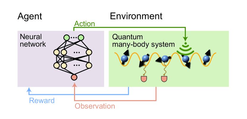
Figure 1: A graphical illustration of the deep RL framework to prepare thermal and prethermal pure quantum states for thermodynamic ensembles. The agent represented by the deep NN is trained to discover a policy that maximizes the cumulative reward, which is computed based on the local observables of the quantum many-body system (environment). At each time step, the NN takes the result of observation as input and outputs the action-value function, from which the action (or the control operation) on the environment is determined. In this work, the action is chosen from a set of unitaries that are presumably available in the preparation protocol.

Having bridged between the notions in quantum control and RL, we can train the NN-based agent to find the best control on the quantum system via searching for an approximation of the optimal action-value function $Q^{*}(o,a)$ (1). Note that the evolution of the quantum state may either be experimentally implemented or numerically simulated, as long as the reward function for the deep RL agent can be readily obtained. Once the training is completed, we determine the preparation protocol as $\{a^{*}_{t}\}_{t}$ by choosing the actions so that $a^{*}_{t}=\operatorname*{arg\,max}_{a}Q(o_{t},a)$ at each time step $t$, which maximizes the reward.

III.2 Local state preparation

We are now ready to describe the preparation protocol for thermal and prethermal pure quantum states that relies solely on local observables, instead of querying for costly global features such as the fidelity. Below, as opposed to global state preparation, we refer to the following scheme as local state preparation.

The central idea of local state preparation is to leverage the typicality of pure quantum states [57, 58, 7, 59]. Typicality refers to the fact that the overwhelming majority of pure quantum states with the same local conserved quantities are indistinguishable means of local observables. Such states are also deemed to be macroscopically indistinguishable. It is natural to expect that, by utilizing the typicality, we can prepare a state that encodes the macroscopic properties of the equilibrium states solely by controlling the local observables. Specifically, we perform local preparation by making the expectation values of the local observables close to the equilibrium state and then letting the system relax to equilibrium through a unitary evolution, without any control.

We may utilize various forms of reward to learn the local observables of the target ensemble. In this work, we formulate the reward function as the inverse of the deviations of the expectation values of the local observables from that of the target states:

$$r_{t}\coloneqq\frac{1}{\left\lvert M_{t}-M_{\mathrm{target}}\right\rvert+\varepsilon},$$ (3)

where $M_{t}=(\braket{O_{1}}_{t},\braket{O_{2}}_{t},\ldots)$ and $M_{\mathrm{target}}=(\braket{O_{1}}_{\mathrm{target}},\braket{O_{2}}_{\mathrm{target}},\ldots)$ are vectors consisting of expectation values $\braket{O}_{t({\rm target})}:={\rm Tr}[\rho_{t({\rm target})}O]$. The small constant $\varepsilon$ is also introduced to prevent divergence of the reward function.

As a concrete target for the demonstration of our local preparation protocol, we choose Gibbs ensembles and GGEs as illustrative examples. The evolution of the quantum many-body state is numerically simulated in an exact manner, while in principle we may also employ approximate methods that rely on, e.g., a variational representation such as tensor networks or neural networks. Alternatively, one may implement the proposed protocol directly on an experimental device as well. In the following, we proceed to describe the detailed properties of the thermodynamic ensembles and the expected preparation efficiency in the presence of typicality.

III.2.1 Gibbs ensemble for non-integrable systems

Let us consider a non-integrable system with the energy being the only local conserved quantity such that its equilibrium is described by a Gibbs ensemble. On a related point, pure states belonging to a given microcanonical shell of the system share their macroscopic properties. This class of typicality is referred to as canonical typicality. One of the most prominent examples of canonical typicality can be illustrated by the Haar measure on the space of pure states under some constraint $R$ (e.g., energy) as [58]

$$\braket{\left\lVert\rho_{A}-\Omega_{A}\right\rVert_{1}}\leq\sqrt{\frac{d_{A}^{2}}{d_{R}}},$$ (4)

where $\rho_{A}=\operatorname{Tr}_{\bar{A}}\left[\ket{\psi}\bra{\psi}\right]$ is the reduced density operator obtained by tracing out the the complement of subsystem $A$ for $\ket{\psi}\bra{\psi}$ with Hilbert space dimension $d_{A}$. On the other hand, $\Omega_{A}=\operatorname{Tr}_{\bar{A}}\left[\mathds{1}_{R}/d_{R}\right]$ is the reduced density operator for the projection operator $\mathds{1}_{R}$, i.e., the maximally mixed state in the Hilbert subspace under the constraint $R$ whose dimension is $d_{R}$. Note that the bracket $\braket{\cdot}$ concerns the average with regard to the Haar measure on the constrained Hilbert space, and $\left\lVert A\right\rVert_{1}=\operatorname{Tr}\sqrt{A^{\dagger}A}$.

Equation (4) means that the average distance between a randomly chosen pure state and the maximally mixed state in the constrained Hilbert space decays polynomially with the Hilbert space size as $d_{R}^{-0.5}$, that is, exponentially with the system size in general quantum systems. The indistinguishability of the pure quantum state from the microcanonical ensemble leads us to expect that, once a state is prepared to be within the target energy shell, the prepared state captures the macroscopic properties with an accuracy that improves exponentially with the system size .

We emphasize that the key of local preparation protocol is to encode the prepared state into the target energy shell, which requires more than merely learning the expectation value of the energy. In other words, even if the expectation value is correctly learned, the prepared state may correspond to a superposition of pure states that belong to other energy shells. Such a situation may cause deviation in other physical observables. In this work, we attempt to address this problem by letting the RL agent learn other macroscopic observables in addition to energy. It is in fact highly nontrivial to determine how many observables we need in order to embed the prepared state into the energy shell. We find that for the non-integrable transverse-field Ising chain, it suffices to take only the total magnetization $\sum_{l}\sigma_{l}^{z}/L$ (for the numerical demonstration, see Sec. IV.2).

As another possibly effective method to assure that the prepared state is encoded in the desired energy shell, we propose to incorporate the variance of observables $\braket{O^{2}}_{\rm target}-\braket{O}_{\rm target}^{2}$ into the reward. For instance, it is obvious that the energy variance is suppressed when the prepared state is in the target energy shell. This is actually not limited to the energy; due to the typicality, we may employ any macroscopic observable for this purpose.

III.2.2 Generalized Gibbs ensemble for integrable systems

As opposed to the non-integrable systems, integrable systems have an extensive number of conserved quantities, which are also called integrals of motion (IOM) in the literature. Rather, the equilibrium states in integrable systems are known to be described by GGEs [54]:

$$\rho_{\mathrm{GGE}}=\frac{\exp\left[-\sum_{m}\lambda_{m}\hat{\mathcal{I}}_{m}\right]}{\operatorname{Tr}\left[\exp\left[-\sum_{m}\lambda_{m}\hat{\mathcal{I}}_{m}\right]\right]},$$ (5)

where $\{\hat{\mathcal{I}}_{m}\}$ is the full set of the IOMs, and $\left\{\lambda_{m}\right\}$ is the corresponding set of the Lagrange multipliers which dictates the distribution over the expectation values of the IOMs.

To discuss the typicality in the set of pure states with close expectation values of IOM, the authors of Ref. [71] have introduced the notion of a statistical ensemble called the generalized microcanonical ensemble (GME). In parallel to the ordinary microcanonical ensemble, the GME is constructed by assigning equal weights to all eigenstates whose IOMs are close to some certain values that identify the ensemble. It has been pointed out in Ref. [71] that the standard deviations of the local observables within such “a window of IOM” decay polynomially as

$$\sigma_{\mathrm{\rm loc}}\propto L^{-0.5},$$ (6)

where $L$ is the system size. Therefore, by following a parallel discussion as in the case for Gibbs ensembles in non-integrable systems, we may also expect that the local preparation protocol will work for GGEs in integrable systems as well, with its accuracy improving polynomially with the system size.

Let us remark on another supporting argument based on the truncation of GGEs itself. While Eq. (5) takes all possible IOMs into account, we expect that the macroscopic behavior in terms of local observables can be extracted by considering local conserved quantities. As such, here, we aim to capture the truncated alternative of the statistical ensemble by focusing on the local integrals of motion (LIOM). Specifically, we denote the LIOMs that act at most $n+1$ neighboring sites as $\hat{I}_{n}^{\sigma}$, with $\sigma$ denoting some additional label, and we introduce a locality-constrained variant of GGE that is known as truncated GGE (tGGE) [72]:

$$\rho_{\mathrm{tGGE},n_{\mathrm{local}}}=\frac{\exp\left[-\sum_{n=0}^{n_{\mathrm{local}}}\sum_{\sigma}\lambda_{n}^{\sigma}\hat{I}_{n}^{\sigma}\right]}{\operatorname{Tr}\left[\exp\left[-\sum_{n=0}^{n_{\mathrm{local}}}\sum_{\sigma}\lambda_{n}^{\sigma}\hat{I}_{n}^{\sigma}\right]\right]},$$ (7)

which only includes the LIOMs with $n\leq n_{\mathrm{local}}$. It is natural to expect that a tGGE will give a good approximation of $\rho_{\rm GGE}$ in terms of local quantities and, furthermore, that $\operatorname{Tr}_{\bar{A}}\left[\rho_{\mathrm{tGGE},n_{\mathrm{local}}}\right]\approx\operatorname{Tr}_{\bar{A}}\left[\rho_{\mathrm{GGE}}\right]$. For instance, in Ref. [72], the transverse field Ising chain has been investigated in the integrable regime and it has been found that tGGEs approximate the corresponding GGEs when $n_{\rm local}$ is larger than the size of subsystem $A$.

We remark that the local preparation protocol for integrable systems aims to construct a tGGE rather than the original GGE. In this sense, we expect that the validity is not assured for observables with higher $n_{\rm local}$, for which the discrepancy between the GGE and the tGGE is non-negligible. We discuss this point more in detail in Sec. V.2.

IV Application to Gibbs ensembles

IV.1 Model and setup

As a demonstration of the local preparation of thermal pure states described by Gibbs ensembles, we consider the transverse field Ising model on a chain with the periodic boundary condition:

$$\hat{H}_{\mathrm{Ising}}=\sum_{l=1}^{L}\left[J\hat{\sigma}_{l}^{z}\hat{\sigma}_{l+1}^{z}+h\hat{\sigma}_{l}^{z}+g\hat{\sigma}_{l}^{x}\right],$$ (8)

where $\hat{\sigma}_{l}^{x},\ \hat{\sigma}_{l}^{y},\ \hat{\sigma}_{l}^{z}$ are the Pauli operators at site $l$, $L$ is the system size, $J$ is the amplitude of the Ising interaction, and $h~{}(g)$ is the strength of the longitudinal (transverse) magnetic field. In the following, the parameters are fixed as $J=1,\ h=0.8090,\ g=0.9045$ so that the system is non-integrable [73]. As a target state, we aim to prepare a thermal pure quantum state corresponding to the Gibbs ensemble with inverse temperature $\beta=0.2$, where the initial state before any quantum control is taken to be a product state $\Ket{\downarrow\downarrow\cdots\downarrow}$. The total preparation time is fixed as $T=24$ with the time step set as $\delta t=0.1$, which also determines the total time step to be $240$.

The set of action candidates $\{a_{t}\}$ available for the RL agent is given as $\{e^{-iG_{k}\delta t}\}_{k=1}^{6}$, where the time evolution generator $G_{k}$ is chosen from the following six operators:

$$\begin{split}&\hat{H}_{\mathrm{Ising}},\ \sum_{l=1}^{L}J\hat{\sigma}_{l}^{z}\hat{\sigma}_{l+1}^{z}+h\hat{\sigma}_{l}^{z},\ g\sum_{l=1}^{L}\hat{\sigma}_{l}^{x},\ \sum_{l=1}^{L}\hat{\sigma}_{l}^{y},\\ &\sum_{l=1}^{L}\hat{\sigma}_{l}^{x}\hat{\sigma}_{l+1}^{y}+\hat{\sigma}_{l}^{y}\hat{\sigma}_{l+1}^{x},\ \sum_{l=1}^{L}\hat{\sigma}_{l}^{y}\hat{\sigma}_{l+1}^{z}+\hat{\sigma}_{l}^{z}\hat{\sigma}_{l+1}^{y}.\end{split}$$ (9)

These terms are also used in Ref. [44], which discusses how to accelerate the preparation of the ground state using counter-diabatic driving. Regarding the local reward $r_{t}$, we include the energy density $L^{-1}\hat{H}_{\mathrm{Ising}}$ and the magnetization density $L^{-1}\sum_{l}\hat{\sigma}_{l}^{z}$. Note that these are the sum of local operators acting on two neighboring sites at most.

IV.2 Numerical results

Figure 2: (a) The learning curves for local preparation of the Gibbs ensemble of the transverse field Ising model in the non-integrable regime. The blue and red curves denote the total reward and the deviation of the energy density computed for the prepared states, respectively. The horizontal axis shows the number of parameter updates. (b) The optimal action sequence $\{a_{t}^{*}\}$ for local preparation of the Gibbs ensemble discovered by the RL agent whose training profile is provided in Fig. 2 (a). The six-fold action indices correspond to 0: $\hat{H}_{\mathrm{Ising}}$, 1: $\sum_{l}J\hat{\sigma}_{l}^{z}\hat{\sigma}_{l+1}^{z}+h\hat{\sigma}_{l}^{z}$, 2: $g\sum_{l}\hat{\sigma}_{l}^{x}$, 3: $\sum_{l}\hat{\sigma}_{l}^{y}$, 4: $\sum_{l}\hat{\sigma}_{l}^{x}\hat{\sigma}_{l+1}^{y}+\hat{\sigma}_{l}^{y}\hat{\sigma}_{l+1}^{x}$, 5: $\sum_{l}\hat{\sigma}_{l}^{y}\hat{\sigma}_{l+1}^{z}+\hat{\sigma}_{l}^{z}\hat{\sigma}_{l+1}^{y}$, respectively. After quickly manipulating the macroscopic observables to encode the properties of the thermal ensemble, the agent mainly chooses to evolve the system under the target Hamiltonian $\hat{H}_{\rm Ising}$. For all plots, the system size is $L=16$ with the inverse temperature set as $\beta=0.2$.

We now proceed to present numerical results that successfully prepare thermal pure quantum states, which encode both the local observables used during the training and also more non-local ones that are excluded from the reward function. Figure 2 (a) shows an example of the learning curve of the RL agent for $L=16$. We can see that, as the number of training episodes increases, the RL agent learns the better protocols that achieve higher total reward and smaller energy deviation.

Here, we briefly discuss the control protocol found by the RL agent. Figure 2 (b) shows the control protocol whose learning curve is shown in Fig. 2 (a) to realize a thermal pure state described by the Gibbs ensemble. It can be seen that the optimal protocol consists of two stages: first is the sequence of nontrivial actions that change macroscopic observables, and the second is the relaxation of the system under free evolution using $\hat{H}_{\rm Ising}$, which leads the system to the typical state of $\hat{H}_{\rm Ising}$. While there is a small number of actions other than the free relaxation at the late stage of the control protocol, we argue that they do not contribute significantly to the result even if we substitute them with $\hat{H}_{\rm Ising}$ because they consist almost entirely of the alternating use of actions 1 and 2. This can be considered to be effectively equivalent to $\hat{H}_{\rm Ising}$ in the sense of the Trotter decomposition.

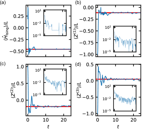
Figure 3: (a)–(d) The dynamics of the local observables generated by the state preparation protocol learned by the deep RL agent, with the insets showing the absolute error from the corresponding expectation values of the target Gibbs state (red line). Each panel displays (a) energy density $\hat{H}_{\mathrm{Ising}}/L$, (b) $Z^{(1)}/L=L^{-1}\sum_{l}\hat{\sigma}_{l}^{z}$, (c) $Z^{(2)}/L=L^{-1}\sum_{l}\hat{\sigma}_{l}^{z}\hat{\sigma}_{l+1}^{z}$, and (d) $Z^{(3)}/L=L^{-1}\sum_{l}\hat{\sigma}_{l}^{z}\hat{\sigma}_{l+1}^{z}\hat{\sigma}_{l+2}^{z}$. Note that the local observables in (a) and (b) are both included in the reward for the deep RL agent. We observe convergence not only for physical quantities that are included in the RL reward as in (a) and (b), but also for local observables that are absent from the reward, as in (c) and (d). For all plots, the system size is $L=16$, with the inverse temperature set as $\beta=0.2$.

Figures 3 (a)–(d) display the dynamics of the local observables obtained by the preparation protocol learned by the RL agent. Figures 3 (a) and (b) show the observables $\hat{H}_{\mathrm{Ising}}$ and $\sum_{l}\hat{\sigma}_{l}^{z}$, respectively, which are used for the reward function. Both of them converge to the corresponding values of the Gibbs ensemble represented by the red horizontal lines. It is more intriguing to see the convergent behaviors in Figs. 3 (c) and (d), which show the dynamics of local observables that are not included in the reward function, namely, the two-point correlator $\sum_{l}\hat{\sigma}_{l}^{z}\hat{\sigma}_{l+1}^{z}$ and the three-point correlator $\sum_{l}\hat{\sigma}_{l}^{z}\hat{\sigma}_{l+1}^{z}\hat{\sigma}_{l+2}^{z}$, respectively.

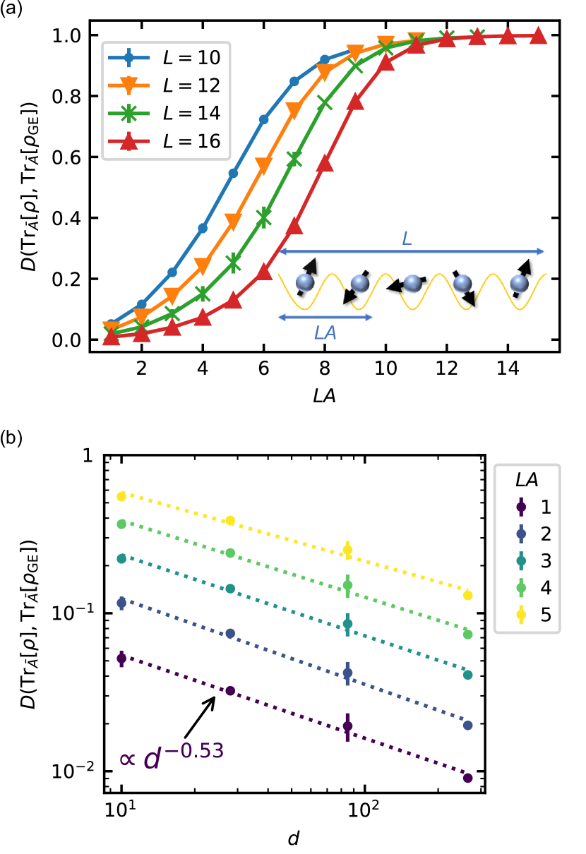
Figure 4: The distances between the reduced density operators of the target Gibbs state and the prepared state, which are averaged over time and random training instances. (a) The error in the distance function $\bar{D}$ at various subsystem sizes $LA$. The blue circles, orange inverted triangles, green crosses, and red normal triangles denote the data for $L=10,12,14,16$, respectively. (b) The decay of the error in the reduced density operator along with the corresponding energy shell dimension $d$, i.e., the number of eigenstates in the energy shell. The dotted lines are guides to the eye showing the fits with $D=ad^{-b}$, where the powers $b$ are summarized in Table 3 of Appendix. B. The error bars correspond to the standard deviations of different protocols learned independently with random seeds. In both plots, the system is controlled by the deep RL agent at $0\leq t\leq 24$, and then undergoes free evolution $\exp[-i\hat{H}_{\mathrm{Ising}}t]$ in $24<t\leq 48$. Note that the distance $\bar{D}$ concerns the average over the free evolution period and also the random training instance.

It is natural to wonder how accurately the general observables, or the reduced density operators of the local systems, are captured by the local preparation protocol. For this purpose, we evaluate the distance between the reduced density operators of the prepared pure state and the target Gibbs ensemble as

$$D(\rho,\rho^{\prime})\coloneqq\frac{\left\lVert\rho-\rho^{\prime}\right\rVert_{\mathrm{F}}}{\sqrt{\left\lVert\rho\right\rVert_{\mathrm{F}}^{2}-\left\lVert\rho^{\prime}\right\rVert_{\mathrm{F}}^{2}}},$$ (10)

where $\left\lVert A\right\rVert_{\mathrm{F}}\coloneqq\sqrt{\operatorname{Tr}\left[A^{\dagger}A\right]}$ is the Frobenius norm .

We can see from Fig. 4 (a) that the time average of the distance function given in Eq. (10), which we denote as $\bar{D}$, is suppressed for the smaller subsystem size $LA$. What is more interesting is the scaling with respect to the total system size; we observe nontrivial suppression of error along with the increase of the system size $L$.

We go further into the scaling of the error suppression by performing finite-size scaling on the averaged distance function as shown in Fig. 4 (b). Here, we observe that the scaling of the suppression is given as

$$\bar{D}=\mathcal{O}(d^{-b}),$$ (11)

where $d$ is the dimension of the corresponding energy shell. To be specific, $d$ is obtained by counting the number of eigenstates included within the energy window $[\braket{\hat{H}_{\mathrm{Ising}}}_{\beta}-\varepsilon_{\mathrm{e}}L,~{}\braket{\hat{H}_{\mathrm{Ising}}}_{\beta}]$, where $\braket{\hat{H}_{\mathrm{Ising}}}_{\beta}$ is the energy expectation value of the target Gibbs ensemble at inverse temperature $\beta$, and the shell width is fixed as $\varepsilon_{\mathrm{e}}=0.5$ (for further discussion on the choice of $\varepsilon_{\mathrm{e}}$, see Appendix C).

The scaling of the distance given in Eq. (11) implies that $\bar{D}$ decays exponentially with the system size $L$. We argue that this is compatible with the scaling of canonical typicality, given in Eq. (4). This feature supports an expectation that our local preparation protocol for the Gibbs ensembles becomes exponentially more precise as the system size increases.

As a technical remark, we mention that the dimension shown in the figure corresponds to the size of the symmetry-resolved Hilbert space, namely the parity and the momentum.

V Application to generalized Gibbs ensemble

V.1 Model and setup

We next describe an even more intriguing system that is integrable so that the thermodynamic ensembles is described by GGEs. Specifically, we consider the XX model on a periodic chain with a longitudinal field:

$$\hat{H}_{\mathrm{XX}}=-\sum_{l=1}^{L}\left[\frac{J}{2}\left(\hat{\sigma}_{l}^{x}\hat{\sigma}_{l+1}^{x}+\hat{\sigma}_{l}^{y}\hat{\sigma}_{l+1}^{y}\right)+h\hat{\sigma}_{l}^{z}\right],$$ (12)

where $J$ is the amplitude of interaction, $h$ is the strength of the magnetic field along the $z$-axis and $L$ is the system size. In the following, the parameters are fixed as $J=1$ and $h=2$.

The integrability of the XX model can be verified straightforwardly by mapping into a non-interacting fermionic system via the Jordan-Wigner transformation:

$$\hat{H}_{\mathrm{XX}} = -\sum_{l=1}^{L}[J(\hat{a}_{l}^{\dagger}\hat{a}_{l+1}+\hat{a}_{l+1}^{\dagger}\hat{a}_{l})+2h(\hat{a}_{l}^{\dagger}\hat{a}_{l}-\frac{1}{2})],$$ (13)

$$= -\sum_{k}\left[2\left\lparen J\cos k+h\right\rparen\hat{n}_{k}-h\right],$$ (14)

where $\hat{a}_{l}^{\dagger}$ and $\hat{a}_{l}$ are fermionic creation and annihilation operators that are related to the Pauli operators as $\hat{a}_{l}^{({\dagger})}=\prod_{l^{\prime}<l}\hat{\sigma}_{l^{\prime}}^{z}\hat{\sigma}_{l}^{+(-)}$, where $\hat{\sigma}_{l}^{\pm}=(\hat{\sigma}_{l}^{x}\pm i\hat{\sigma}_{l}^{y})/2$. In the second row of Eq. (14), we move into the Fourier space by introducing the mode occupation operator $\hat{n}_{k}=\hat{a}_{k}^{\dagger}\hat{a}_{k}$ for $\hat{a}_{k}=L^{-1/2}\sum_{l}\hat{a}_{l}e^{-ikl}$. We can construct as many LIOMs as the system size $L$ by taking the linear combination as

$$\hat{I}_{n}^{+} =-2J\sum_{k}\cos{(nk)}\hat{a}_{k}^{\dagger}\hat{a}_{k}=-J\sum_{l}\left\lparen\hat{a}_{l}^{\dagger}\hat{a}_{l+n}+\hat{a}_{l+n}^{\dagger}\hat{a}_{l}\right\rparen,$$

$$\hat{I}_{n}^{-} =-2J\sum_{k}\sin{\left\lparen nk\right\rparen}\hat{a}_{k}^{\dagger}\hat{a}_{k}=iJ\sum_{l}\left\lparen\hat{a}_{l}^{\dagger}\hat{a}_{l+n}-\hat{a}_{l+n}^{\dagger}\hat{a}_{l}\right\rparen.$$

For convenience in the later discussion, we mention the rightmost sides to remark that $\hat{I}_{n}^{\pm}$ can be explicitly expressed as sums over hopping terms between the $n$-th nearest neighboring sites in the fermionic picture.

As the target thermodynamic ensemble, we aim for the GGE constructed from the LIOMs as

$$\rho_{\mathrm{GGE}}=\frac{\exp\left[-\sum_{n}\sum_{\sigma=\pm}\lambda_{n}^{\sigma}\hat{I}_{n}^{\sigma}\right]}{\operatorname{Tr}\left[\exp\left[-\sum_{n}\sum_{\sigma=\pm}\lambda_{n}^{\sigma}\hat{I}_{n}^{\sigma}\right]\right]},$$ (15)

where $\{\lambda_{n}^{\sigma}\}$ are the Lagrange multipliers. More precisely, we set the initial state of the control system to be the ground state of $\hat{H}_{\mathrm{tb}}$ in the space of the total particle number $N_{\mathrm{f}}$, and aim to prepare a prethermal pure state corresponding to a given set of Lagrange multipliers $\{\lambda_{n}^{\sigma}\}$ (for details regarding the parameter choice of $\{\lambda_{n}^{\sigma}\}$, see Appendix D). The total preparation time is fixed as $T=40$ and the time step as $\delta t=0.2$; thus the total number of time steps is $200$.

In parallel with the case for Gibbs ensembles, we allow the deep RL agent to choose $a_{t}$ as an appropriate unitary from a set $\{e^{-iG_{k}\delta t}\}_{k=1}^{15}$, where the time evolution generator $G_{k}$ is chosen from the following 15 operators:

$$\begin{split}&\hat{H}_{\mathrm{XX}},~{}\sum_{l=1}^{L}\hat{a}_{l}^{\dagger}\hat{a}_{l}\cos\frac{m\pi}{L}l,~{}\sum_{l=1}^{L}\hat{a}_{l}^{\dagger}\hat{a}_{l}\sin\frac{m\pi}{L}l,\\ &\sum_{l=1}^{L}\left\lparen\hat{a}_{l}^{\dagger}\hat{a}_{l+j}+\hat{a}_{l+j}^{\dagger}\hat{a}_{l}\right\rparen\cos\frac{n\pi}{L}l,\\ &\sum_{l=1}^{L}\left\lparen\hat{a}_{l}^{\dagger}\hat{a}_{l+j}+\hat{a}_{l+j}^{\dagger}\hat{a}_{l}\right\rparen\sin\frac{n\pi}{L}l,\end{split}$$ (16)

where $m\in\{2,4,L\}$, and $\left\lparen j,n\right\rparen\in\{\left\lparen 1,2\right\rparen,\left\lparen 2,2\right\rparen,\left\lparen 1,L\right\rparen,\left\lparen 2,L\right\rparen\}$. Note that these operators are chosen so that they are not diagonal in the position or momentum basis.

Regarding the local reward $r_{t}$, we employ normalized LIOMs ${\{\hat{I}_{n}^{+}/L\}}_{1\leq n\leq n_{\mathrm{local}}}$, where we fix $n_{\rm local}=4$ in the following. All $\hat{I}_{n}^{-}$ terms are excluded since they are constantly zero not only for the initial and target states, but also for any intermediate states $\rho_{t}$ evolved with the above unitaries.

V.2 Numerical results

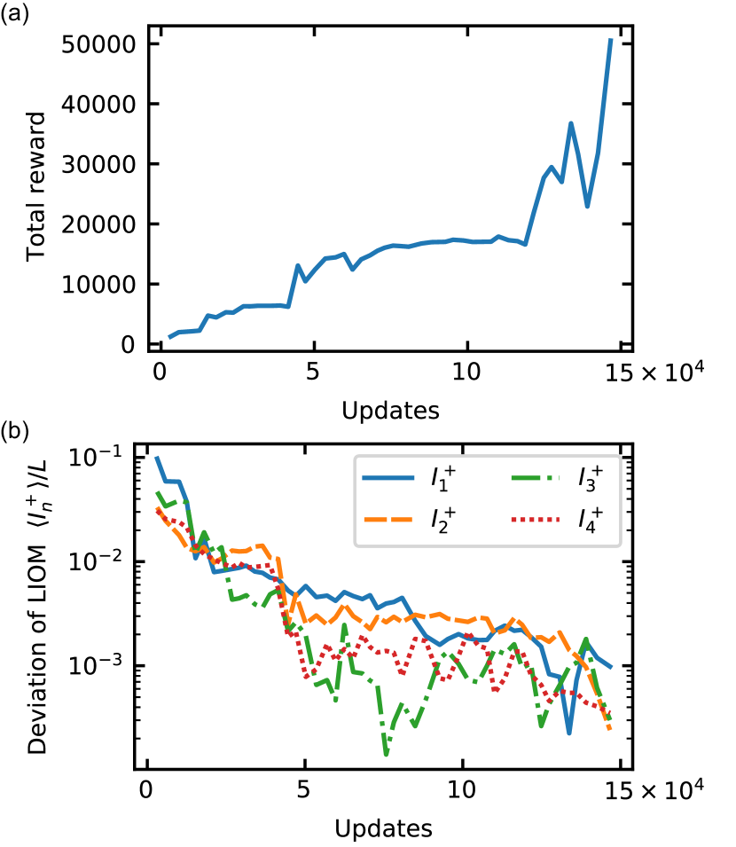
Figure 5: The learning curves for local preparation of the GGE. These figures show the total rewards and the deviations of the LIOM densities at the end of the episodes in evaluating the training progress. The horizontal axis shows the number of parameter updates. (a) The total rewards. (b) The deviations of the LIOM densities. The corresponding model is the transverse field Ising model where the parameter is set so that the model is integrable. We add the LIOMs $\hat{I}_{n}^{+}$ with separation $n=1,2,3,4$ to the reward of RL. The system size $L=120$. The lines show the median of the corresponding values in evaluation with random seeds.

We now present the numerical results obtained by running the deep RL algorithm to prepare prethermal pure quantum states that capture the characteristics of the GGE. As we show in the learning curve in Fig. 5(a), the deep RL agent successfully learns to improve the local preparation protocol. This can be more quantitatively understood from Fig. 5(b), which evaluates the absolute difference in the expectation values of LIOMs between the target GGE and the prepared state.

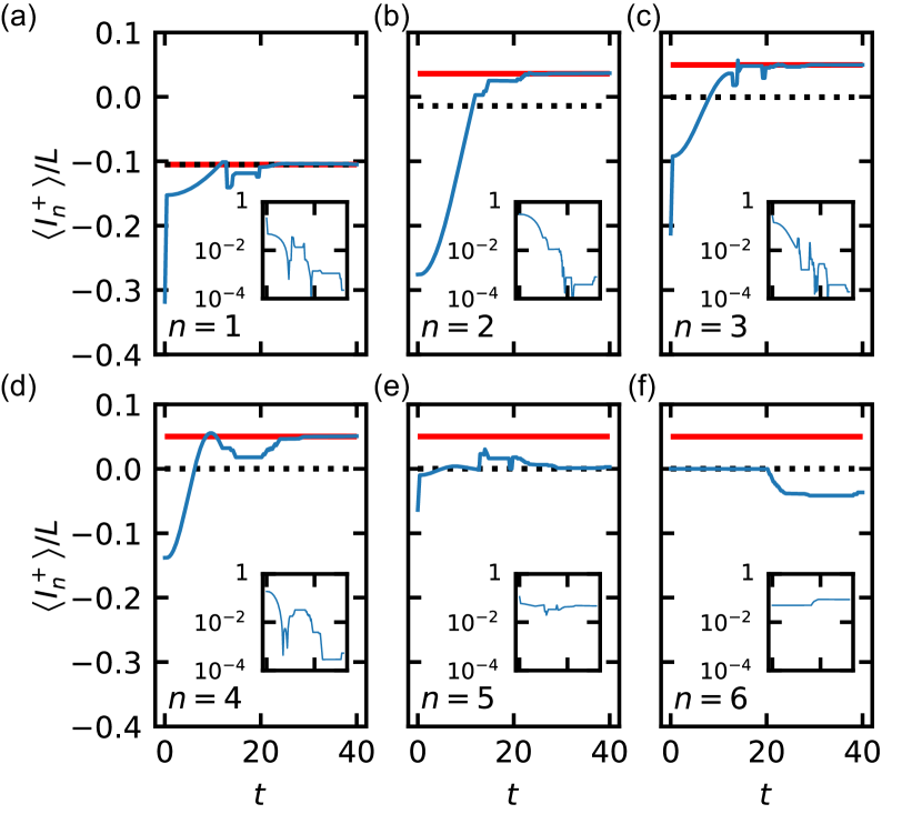
Figure 6: The expectation values of the LIOMs in the protocol found by RL for the GGE (blue). Each panel shows the LIOM with different separations. The red horizontal lines show the corresponding expectation values of the target GGE. The dotted black lines represent the relevant Gibbs ensemble, which shares the same expectation values of the total particle number and the energy. The insets show the absolute deviations in the expectation values $\langle\hat{I}_{n}^{+}\rangle/L$ between the states in the protocol and the target GGE. We add the LIOMs $\hat{I}_{n}^{+}$ with separation $n=1,2,3,4$ to the reward of RL. Only LIOMs with separation $n\leq 4$ converge to the expectation values of the GGE.

Let us further investigate the dynamics of the LIOMs generated by the preparation protocol discovered by the RL agent. As shown in Fig. 6, the behavior of the LIOMs seem to be qualitatively different depending on $n$ in the sense that, the only LIOMs with separation $n\leq n_{\mathrm{local}}=4$, which we add to the reward, seem to converge to the expectation values of the GGE.

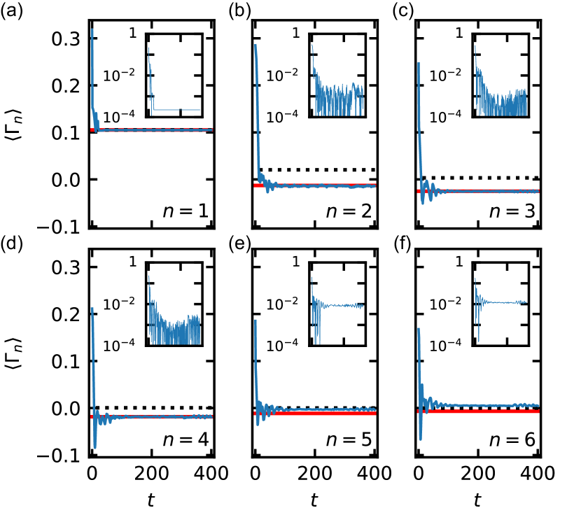
Figure 7: The relaxation processes of the expectation values of the correlation functions given in Eq. (17), which are non-conserved quantities of $\hat{H}_{\mathrm{XX}}$ (12) (blue). Each panel shows the correlation function with different separation $n$, which means the correlation function corresponds to the two spins separated by $n-1$ sites. The red horizontal lines show the corresponding expectation values of the target GGE, whereas the dotted black lines represent the relevant Gibbs ensemble that shares the same expectation values of the total particle number and the energy. Note that the system is controlled with the learned protocol in $0\leq t\leq 40$, and subsequently undergoes free evolution with $\hat{H}_{\mathrm{XX}}$. The only correlation functions with separation $n\leq 4$ fluctuate around the expectation values of the GGE. Note that the correlation function with $n=1$, where the Jordan-Wigner string does not appear, is proportional to the LIOM with $n=1$, i.e., it is the conserved quantity of $\hat{H}_{\mathrm{XX}}$.

Similar behavior can also be observed for non-conserved quantities such as the correlation function

$$\Gamma_{n}\coloneqq\frac{1}{L}\sum_{l}\left\lparen\hat{\sigma}_{l}^{+}\hat{\sigma}_{l+n}^{-}+\hat{\sigma}_{l+n}^{+}\hat{\sigma}_{l}^{-}\right\rparen,$$ (17)

which can be seen as a representative of the local operators acting on neighboring $n+1$ sites. As we can see in Fig. 7, there is a notable convergence into the GGE values for $n\leq n_{\rm local}$, while the errors seem to remain for $n>n_{\rm local}$.

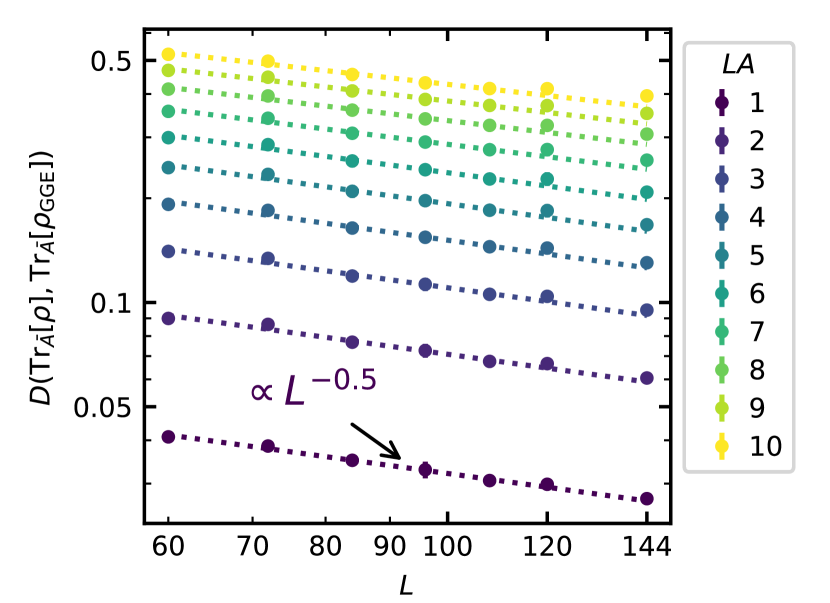
Figure 8: Finite-size scaling of the distance function of the reduced density operators between the prepared states and the target GGE. The dotted lines are guides to the eye that show the power-law fitting $\bar{D}=\mathcal{O}(L^{-b})$, where the powers $b$ are summarized in Table 4 of Appendix. B. The error bars correspond to the standard deviations of different protocols learned independently with random seeds. The system is controlled by the deep RL agent at $0\leq t\leq 40$, and then undergoes free evolution by $\hat{H}_{\mathrm{XX}}$. Note that the distance $\bar{D}$ concerns the average over time, i.e., the free evolution period, and the random training instance. The number of random seeds is five at most.

Furthermore, we focus on the scaling of the error suppression. As we can observe from the finite-size scaling of the averaged distance function $\bar{D}(\rho_{t},\rho_{\rm GGE})$ in Fig. 8, the distance between the reduced density operators is suppressed as $\bar{D}=\mathcal{O}(L^{-b})$. This behavior is compatible with the scaling of the fluctuation of local observables in the GME, given in Eq. (6).

Here, we conjecture that while the errors for $LA\lesssim n_{\rm local}+1$ are suppressed polynomially even for larger system sizes, the errors for $LA\gtrsim n_{\rm local}+1$ may saturate at finite values. This is because the current local preparation scheme learns the LIOMs $\hat{I}_{n}^{\sigma}$ with $n\leq n_{\rm local}$ to encode the prepared state into the “LIOM shell” only for such conserved quantities. This means that the prepared state fully encodes the macroscopic properties of the tGGE but not those of the GGE. We numerically find that the distance between the tGGE and the GGE remains finite even if the total system is at the thermodynamic limit [See Appendix E], which is in agreement with Ref. [72], which has investigated the integrable region of the transverse-field Ising chain. This supports our conjecture that the distance between the GGE and the local-prepared state is not suppressed in the thermodynamic limit. Meanwhile, it is possible that the error from the tGGE itself is suppressed polynomially.

VI Conclusion

In this work, we propose a deep-RL-based quantum state preparation framework for thermodynamic ensembles that relies solely on a few local observables but not on global features such as the fidelity. The core idea is to leverage the typicality of pure states in quantum many-body systems; the macroscopic properties can be encoded simply via learning a few local observables and undergoing free evolution. We provid numerical demonstrations in which the deep RL agent is successfully trained to learn the macroscopic properties of the Gibbs ensembles (Fig. 2) and the GGEs (Fig. 5). We find that the accuracy of the prepared state improves exponentially with the system size for the former (Fig. 4) and polynomially for the latter (Fig. 8), which is consistent with the argument of typicality within a given shell of local conserved quantities.

We envision four future directions for our work. First, the application to interacting integrable models is an important issue for local preparation. This issue is related to the previous work on which conserved quantities should be considered to predict the local properties of the steady state in interacting integrable systems, which can be solved using the Bethe ansatz (see, e.g., Ref. [75]). Based on the prior work, we can expect to be able to perform local preparation if we also include quasi-local conserved quantities in the reward. Note that in such systems, the finite-size effect on the fluctuation of local observables is severe in system sizes that are tractable by exact diagonalization. How to simulate interacting integrable systems efficiently in a scalable way so that a local preparation strategy can be pursued is an open problem.

The second important question is the generalization of the local preparation protocol to include, e.g., dissipative terms, measurement and feedback, or postselection. We naturally expect that the powerful explorability of the deep RL framework is not limited to coherent control but could be applied to broader operation sets.

Third, we may consider the application of the local preparation protocol for the task of Hamiltonian learning [76, 77, 78] by attempting to encode the macroscopic properties using unitaries that do not explicitly contain information about the Hamiltonian itself.

Finally, it is intriguing to investigate how the local preparation protocol is affected by various noises, such as the statistical noise that accompanies sampling over observables. Efficient estimation methods such as randomized measurement schemes [79] will be essential to boost the training accuracy of the RL agent.

VII Acknowledgments

The authors wish to thank fruitful discussion with Ryusuke Hamazaki and Jiahao Yao. S. B. is supported by Materials Education rogram for the future leaders in Research, Industry, and Technology (MERIT) of The University of Tokyo. N.Y. wishes to acknowledge JST PRESTO No. JPMJPR2119 and JST Grant Number JPMJPF2221. Y.A. acknowledges support from the Japan Society for the Promotion of Science (JSPS) through Grant Nos. JP19K23424 and JP21K13859. T.S. is supported by JSPS KAKENHI Grant Number JP19H05796, JST CREST Grant Number JPMJCR20C1, Japan, and JST ERATO-FS Grant Number JPMJER2204, Japan. N.Y. and T.S. are also supported by Institute of AI and Beyond of The University of Tokyo. We implemented the exact time evolution in Sec. IV with QuSpin [80, 81] and the RL algorithm with PyTorch [82]. The RL in Sec. V is performed on AI Bridging Cloud Infrastructure (ABCI) of National Institute of Advanced Industrial Science and Technology (AIST).

Appendix A Layout of the neural network and hyperparameters

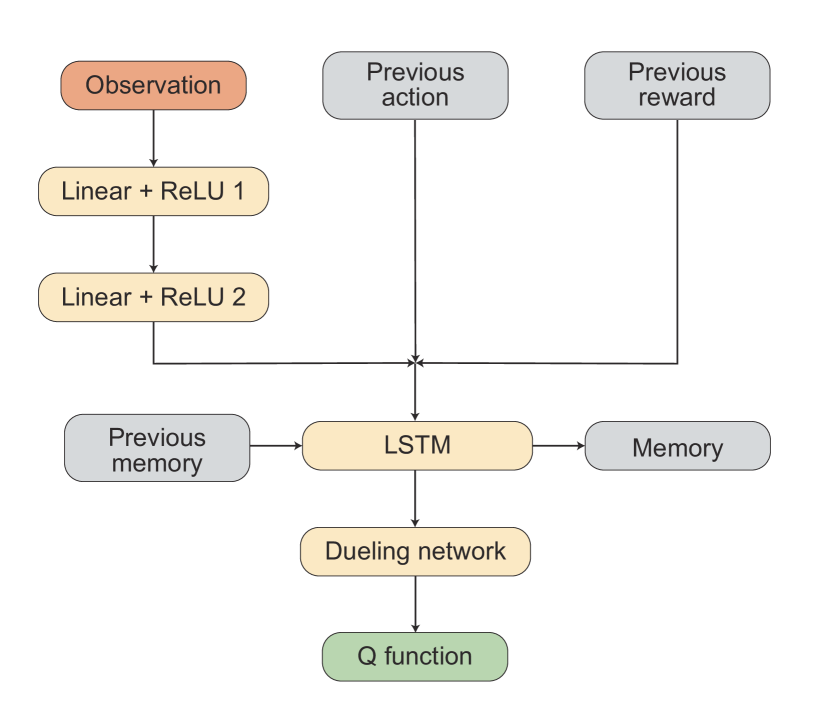
Figure A1: The abstract deep NN architecture used for RL in the present work. At each time step $t$, the deep NN takes as input the observation $o_{t}$, the previous action $a_{t-1}$, and the previous reward $r_{t-1}.$ After intermediate computations by fully connected layers, LSTM, and the dueling network, the deep NN outputs the estimate of the Q function.

	Sec. IV	Sec. V
Linear + ReLU 1	$240\rightarrow 512$	$200\rightarrow 1024$
Linear + ReLU 2	$512\rightarrow 512$	$1024\rightarrow 1024$
LSTM	$(512,6,1)\rightarrow 512$	$(1024,15,1)\rightarrow 1024$
Dueling network	$512\rightarrow 6$	$1024\rightarrow 15$

Table 1: The input and output sizes of each layer are shown as the values preceding and following the arrows, respectively. The input of the NN consists of the action history, the one-hot representation of the previous action, and the previous reward. The input of the “Linear + ReLU 1” layer is only the action history. The one-hot representation of the previous action and the previous reward is concatenated with the output of “Linear + ReLU 2” before the LSTM layer.

Reward discount $\gamma$		0.997
Minibatch size		324(Sec. IV)
		380(Sec. V)
Sequence length		40
Optimizer		Adam [83]
Optimizer setting	Learning rate	$10^{-4}$
	$\varepsilon$	$10^{-3}$
	$\beta$	$(0.9,0.999)$
Replay ratio		1
Gradient norms clip		80

Table 2: The hyperparameters used in the NNs. The agent performs updates on batches of $(\text{minibatch size}\times\text{sequence length})$ observations. The replay ratio means the effective number of times that each experienced observation is being replayed for training purposes. For the details of the hyperparameters, see Ref. [67] and its previous non-LSTM version, Ref. [84]. The other parameters follow thosed used in Ref. [66].

Here, we describe the architecture of the deep NN that is used to estimate the action-value function (Q function). Figure A1 shows the overall picture; the input for the LSTM at time step $t$ is the observation $o_{t}$, the previous action $a_{t-1}$, and the previous reward $r_{t-1}$, whereas the output is Q function whose optimal expression is given in Eq. (1) in the main text. Refer to Table 1 for the size of the input and output of each layer and Table 2 for the hyperparameter used in the NN. In the following, we further describe the details of the structure.

The observation $o_{t}$ is chosen to be the action history $o_{t}=\left\lparen a_{0},a_{1},\ldots,a_{t-1},-1,\ldots,-1\right\rparen$, which is fed to the fully connected layers. fully connected layers first perform linear transformation, and then apply a non-linear activation function which is chosen to be the rectified linear unit (ReLU) in the present work. The intermediate output from the second fully connected layer is concatenated with the previous choice of action $a_{t-1}$ and the reward in the previous time step $r_{t-1}$, and then fed to the LSTM layer.

The LSTM layer is introduced so that the network can refer to the history of the computational results at $t^{\prime}<t$ to estimate the Q function at time step $t$. Namely, the input of the LSTM layer is not only the one mentioned above but also its ”memory”, including a hidden state (short-term memory) and a cell state (long-term memory) [69]. Refer to literature such as Ref. [85] for detailed information. This output memory is fed to the LSTM layer in the next time step $t$, which enables the deep NN to successfully deal with time-series inputs.

In the subsequent dueling network [86], the input is separated into two branches. One branch evaluates the value of the observation $V(o)$, and the other branch evaluates the advantage of actions regarding the observation $A(o,a)=Q(o,a)-V(o)$. The output Q function of the dueling network is obtained by summing the outputs of the two branches: $Q(o,a)=V(o)+A(o,a)$. This separation may contribute to better training stability, faster convergence, and better performance.

As a computational resource, we use a single CPU and four GPUs (Intel Xeon E5-2698 v4, $4\times$NVIDIA Tesla V100) in Sec. IV and two CPUs and four GPUs ($2\times$Intel Xeon Gold 6148, $4\times$NVIDIA Tesla V100) in Sec. V, respectively.

Appendix B Fitting parameters for the finite-size scaling of the preparation accuracy

In Tables 3 and 4, we summarize the powers $b$ obtained by the fit for the finite-size scaling of the local preparation accuracy in Sec. IV.2 and Sec. V.2, respectively.

Subsystem size $LA$	Power $b$
1	0.53(4)
2	0.54(4)
3	0.51(4)
4	0.48(4)
5	0.43(4)

Table 3: The powers obtained by the fit for the result of the finite-size scaling of the distance function $\bar{D}$, given by Eq. (10), between the prepared states and the target Gibbs ensembles for the system size $L=10,12,14,16$ in Sec. IV.2.

subsystem size $LA$	power $b$
1	0.50(3)
2	0.50(5)
3	0.46(4)
4	0.43(4)
5	0.41(4)
6	0.41(3)
7	0.41(3)
8	0.41(3)
9	0.41(3)
10	0.41(3)

Table 4: The powers obtained by the fit for the result of the finite-size scaling with the system size $L=60,72,84,96,108,120$ for the distance function $\bar{D}$, given by Eq. (10), between the prepared states and the target GGE in Sec. V.2.

Appendix C Relationship between energy shell width $\varepsilon_{\rm e}$ and scaling of preparation accuracy

Here, we discuss the relationship between the energy shell width $\varepsilon_{\mathrm{e}}$ and the scaling behavior of the accuracy of the prepared state. Recall that the distance function in Eq. (10) of the main text is given as

$$D(\rho,\rho^{\prime})=\frac{\|\rho-\rho^{\prime}\|_{\rm F}}{\sqrt{\|\rho\|_{\rm F}^{2}-\|\rho^{\prime}\|_{\rm F}^{2}}},$$ (18)

where $\|A\|_{\rm F}=\sqrt{{\rm Tr}[A^{\dagger}A]}$ denotes the Frobenius norm. In Fig. C2, we show how the scaling exponent $b$ defined by $\bar{D}(\rho_{\rm Gibbs},\rho_{t})=O(d^{-b})$ varies according to $\varepsilon_{\mathrm{e}}$. At $\varepsilon_{\mathrm{e}}=0.1$ for $L=10$, the corresponding energy shell only includes a single eigenstate. Meanwhile, $\varepsilon_{\mathrm{e}}=0.75$ corresponds to the extreme case where almost all eigenstates below $\braket{\hat{H}_{\rm Ising}}_{\beta}$ are included in the energy shell $[\braket{\hat{H}_{\rm Ising}}_{\beta}-\varepsilon_{\mathrm{e}}L,\braket{\hat{H}_{\rm Ising}}_{\beta}]$. In Sec. IV.2, we choose intermediate $\varepsilon_{\mathrm{e}}$ so that the power $b$ is stable against the choice of $\varepsilon_{\mathrm{e}}$.

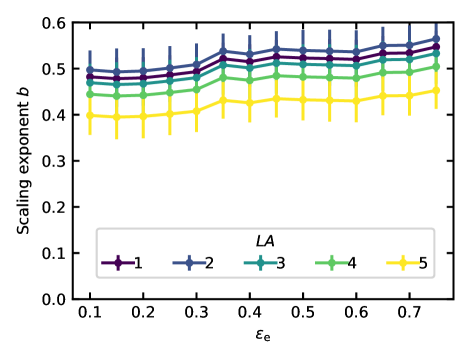
Figure C2: The relationship between the energy shell width $\varepsilon_{\rm e}$ and the scaling exponent $b$ of the distance $\bar{D}$, with regard to the local preparation of the Gibbs ensemble. The parameters of the system are identical to those used in Sec. IV.2.

Appendix D Choosing Lagrange multipliers for the target GGE

The Lagrange multipliers for the GGE in Sec. V is chosen so that the expectation values of local conserved quantities partly reproduce those of the Gibbs ensemble, while some deviate from it. Specifically, we impose the following equalities:

$$\operatorname{Tr}\left[\hat{I}_{n}^{+}\rho_{\mathrm{GGE,target}}\right]=\braket{\hat{I}_{n}^{+}}_{\beta}\ \ \ \,\text{for $n=0,~{}1$},$$ (19)

$$\operatorname{Tr}\left[\hat{I}_{n}^{+}\rho_{\mathrm{GGE,target}}\right]=\braket{\hat{I}_{n}^{+}}_{\beta}+\varepsilon_{\mathrm{I}}L\ \text{for $2\leq n<\frac{L}{2}$},$$ (20)

$$\operatorname{Tr}\left[\hat{I}_{n}^{-}\rho_{\mathrm{GGE,target}}\right]=\braket{\hat{I}_{n}^{-}}_{\beta},$$ (21)

where ${\braket{\hat{I}_{n}^{\sigma}}_{\beta}}$ represents the expectation values of the LIOMs of the Gibbs ensemble at the inverse temperature $\beta=0.4$. Note that $\varepsilon_{\mathrm{I}}$ determines the deviation between the target GGE and the Gibbs ensemble. For simplicity, we consistently take $\varepsilon_{\rm I}=0.05$ for every $L$. In addition, we set $\operatorname{Tr}\left[\hat{I}_{L/2}^{+}\rho_{\mathrm{GGE,target}}\right]=0$ because the fermionic tight-binding Hamiltonian obtained from the Jordan-Wigner transformation (Eq. (13) in the main text) is anti-periodic when the fermionic particle number $N_{\mathrm{f}}$ is even.

We remark that the LIOMs with $n=0,1$ correspond to the total particle number and the energy, respectively. Thus, this target GGE shares only the expectation values of the total particle number and the energy with the Gibbs ensemble. Therefore, in order to prepare the subsystem whose size is larger than 2, we need to control additional LIOMs other than the particle number and energy.

Appendix E The distance between the GGE and the tGGE

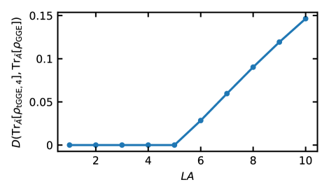
Figure E3: The distance, given by Eq. (10), between the target GGE in Sec. V.2 and the corresponding tGGE with $n_{\mathrm{local}}=4$.

To quantify the difference between the tGGE and the target GGE considered in Sec. V.2, we show the distance $D(\rho_{\rm GGE},\rho_{\rm tGGE})$ in Fig. E3 (see Eq. (10) for the definition). We observe that the tGGE and the GGE agree well when $LA\leq n_{\mathrm{local}}+1$, whereas they deviate when $LA>n_{\mathrm{local}}+1$. This result is compatible with Ref. [72], which considers the integrable parameter region of the transverse-field Ising chain.

Appendix F System-size dependence of learning progress

Figure F4: The system-size dependence of the learning progress for the local preparation of (a) Gibbs ensembles in Sec. IV.2 and (b) GGE in Sec. V.2. These panels show the deviation of (a) the energy density and (b) the LIOM densities, respectively. Each panel represents the average regarding different protocols learned independently to perform the finite-size scaling in Fig. 4 or Fig. 8. The insets show the number of updates required to bring the deviations below a certain threshold of (a) $0.02$ and (b) $0.01$, respectively.

In this section, we analyze the system-size dependence of the progresses of RL. Figure F4 shows the learning curves of physical observables for different system sizes. They tell us that the number of updates required to learn the optimal protocols is almost independent of the system size. We suppose that this feature is related to the fact that our method considers only local properties, which are independent of the system size.

Appendix G Learning for other initial states and unitaries

	Initial state	Generators
(i)	Ground	Same as Sec. IV.2
(ii)	Ground	$\hat{H}_{\mathrm{Ising}},\,\sum_{l=1}^{L}J\hat{\sigma}_{l}^{z}\hat{\sigma}_{l+1}^{z}+h\hat{\sigma}_{l}^{z},\,g\sum_{l=1}^{L}\hat{\sigma}_{l}^{x}$
(iii)	Product	$\hat{H}_{\mathrm{Ising}},\,\sum_{l=1}^{L}J\hat{\sigma}_{l}^{z}\hat{\sigma}_{l+1}^{z}+h\hat{\sigma}_{l}^{z},\,g\sum_{l=1}^{L}\hat{\sigma}_{l}^{x}$
(iv)	Product	$\sum_{l=1}^{L}J\hat{\sigma}_{l}^{z}\hat{\sigma}_{l+1}^{z}+h\hat{\sigma}_{l}^{z},\,g\sum_{l=1}^{L}\hat{\sigma}_{l}^{x}$
(v)	Product	$\sum_{l=1}^{L}\hat{\sigma}_{l}^{z}\hat{\sigma}_{l+1}^{z},\,\sum_{l=1}^{L}\hat{\sigma}_{l}^{z},\,\sum_{l=1}^{L}\hat{\sigma}_{l}^{x}$

Table 5: The choices of the initial state and the unitary generators in Appendix G. Ground means the corresponding initial state of the preparation is the ground state. Product means that the corresponding initial state of the preparation is the product state, which is the same as that used in Sec. IV.2.

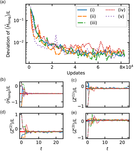
Figure G5: The results of deep RL considering different unitary generators and initial states. The choices of the unitary generators and the initial state are shown in Table 5. (a) The learning curves for local preparation of the Gibbs ensemble of the transverse field Ising model, which is the same as that used in Sec. IV.2. Each of curves (i)–(v) shows the energy deviation calculated for the prepared states by learning corresponding to each choice. The horizontal axis shows the number of parameter updates. (b)–(e) The dynamics of the local observables generated by the state preparation protocol learned by deep RL. The red horizontal lines show the corresponding expectation values of the target Gibbs ensemble. Each panel displays the expectation values as follows: (b) $\hat{H}_{\mathrm{Ising}}/L$, (c) $Z^{(1)}/L=L^{-1}\sum_{l}\hat{\sigma}_{l}^{z}$, (d) $Z^{(2)}/L=L^{-1}\sum_{l}\hat{\sigma}_{l}^{z}\hat{\sigma}_{l+1}^{z}$, and (e) $Z^{(3)}/L=L^{-1}\sum_{l}\hat{\sigma}_{l}^{z}\hat{\sigma}_{l+1}^{z}\hat{\sigma}_{l+2}^{z}$. The system size $L=14$, with the inverse temperature set as $\beta=0.2$.

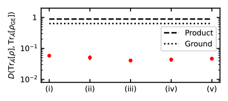
Figure G6: The distance between the reduced density operators whose size is 2 of the prepared states and the target Gibbs state used in Sec. IV.2. The red circles represent the prepared state, taking into consideration the different unitary generators and initial states. The choices of the unitary generators and the initial state are shown in Table 5. The horizontal black dashed line shows the result for the product state which is the same as that used in Sec. IV.2. The horizontal black dotted line represents the ground state. The system size $L=14$.

In this section, we provide the results of deep RL considering different unitary generators and initial states. The choices of the unitary generators and the initial state are shown in Table 5. The target state is the same as in Sec. IV.2 and the system size $L=14$.

Figure G5 (a) shows the learning curves of the RL agent corresponding to choices (i)–(v), respectively. We can see that as the number of training episodes increases, all RL agents corresponding to the different choices learn the better protocols that achieve smaller energy deviation.

Figures G5 (b)–(e) display the dynamics of the local observables obtained by the preparation protocol learned by the RL agent. All of them converge to the corresponding values of the Gibbs ensemble represented by the red horizontal lines.

In Fig. G6, we show the time average of the distance function given in Eq. (10) of the subsystems between the target Gibbs state and the prepared state. The values in these results are comparable to those in Sec. IV.2 and we can conclude that the prepared states under choices (i)–(v) are typical.

Surprisingly, even for choices (iv) and (v), which cannot use $\hat{H}_{\mathrm{Ising}}$, the observables (d) and (e), which are not used for the reward, converge to the target values and the distances between the subsystems become small. We suppose that the unitary time evolutions, which maintain a steady state with respect to the observables added to the reward (the energy and total magnetization), are effectively equivalent to the time evolutions by $\hat{H}_{\mathrm{Ising}}$, which makes the prepared state typical. We point out the connection to the studies [77] where the steady state has embedded Hamiltonian information that can be used to infer the parameters of the Hamiltonian. Of course, this phenomenon may be model-dependent and needs to be verified more precisely.

Appendix H Eigenstate thermalization hypothesis

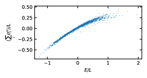
Figure H7: The eigenenergy density dependence of the eigenstate expectation values of $L^{-1}\sum_{l=0}^{L-1}\sigma_{l}^{x}$, that is, we plot $\{\braket{E_{\alpha}}{\sum_{l=0}^{L-1}\sigma_{l}^{x}}{E_{\alpha}}/L\}_{\alpha}$, where $\left\{\ket{E_{\alpha}}\right\}_{\alpha}$ are the eigenstates. The Hamiltonian is $\hat{H}_{\mathrm{Ising}}$, whose parameters are the same as the ones used in Sec. IV.2. We can observe that eigenstates in an energy shell share a typical value, which is a microcanonical ensemble average. Furthermore, these typical values show the nonlinear dependence on the eigenenergy density. The system size $L=16$.

In this section, we briefly describe the eigenstate thermalization hypothesis (ETH), which is about the typical behavior of eigenstates in an energy shell. Furthermore, by looking at the dependence of the eigenstate expectation values of the total magnetization $\sum_{l}\sigma_{l}^{z}/L$ on the eigenstate energy density, we can infer the cause of the successful local preparation by using the total magnetization as an additional local observable of the reward for RL in Sec. IV.2.

The ETH refers to the idea that the energy eigenstates satisfy the canonical typicality [87, 88, 89]. The ETH claims that every energy eigenstate in the energy shell represents thermal equilibrium. More specifically, the energy eigenstates give the same expectation values of macroscopic observables as the relevant microcanonical ensemble for a large system:

$$\braket{E_{\alpha}}{\hat{O}}{E_{\alpha}}\approx\braket{\hat{O}}_{\mathrm{MC}}$$ (22)

for every energy eigenstate $\ket{E_{\alpha}}$ in an energy shell, where $\Braket{\cdot}_{\mathrm{MC}}$ is the corresponding microcanonical ensemble average. Based on the ETH, we can explain the thermalization mechanism of isolated quantum many-body systems [53, 56, 90]. The ETH has been verified numerically for few-body observables in a variety of non-integrable quantum many-body lattice models [73, 91, 92, 93, 94, 95, 96].

In addition, a power-law decay with the dimension of the corresponding energy shell is observed for the variance of the energy eigenstate expectation values in the energy shell:

$$\sigma_{\mathrm{ETH}}^{2}\coloneqq\frac{1}{d}\sum_{\alpha}{\left[\braket{E_{\alpha}}{\hat{O}}{E_{\alpha}}-\braket{\hat{O}}_{\mathrm{MC}}\right]}^{2},$$ (23)

where $d$ is the dimension of the energy shell, that is, the variance decays exponentially with the system size [91].

In Fig. H7, we show the eigenenergy density dependence of the eigenstate expectation values of total magnetization $L^{-1}\sum_{l=0}^{L-1}\sigma_{l}^{x}$, which is the additional local observable of the reward for RL in Sec. IV.2. The Hamiltonian is $\hat{H}_{\mathrm{Ising}}$, whose parameters are the same as those used in Sec. IV.2. Figure H7 shows that the eigenstates in an energy shell have a typical value. This behavior is consistent with the ETH.

As we note in Sec. III.2.1, it is nontrivial to determine how many observables we need to embed the prepared state into a single energy shell. In Fig. H7, we also observe the nonlinear dependence of the typical values on the energy densities. In particular, the dependence appears to be strictly convex. We conjecture that this strict convexity helps the prepared state consist of eigenstates within a single energy shell for our demonstration in the non-integrable transverse-field Ising model.

Appendix I Numerical methods

I.1 Non-integrable systems

For the numerical calculations regarding non-integrable systems, we adopt rigorous standard methods considering the Hilbert space the dimension $d$ of which scales exponentially with the system size. To calculate efficiently, the Hilbert space is resolved by the parity and momentum symmetry. Specifically, the calculation is limited to the zero-momentum sector and the parity-symmetric sector. The time evolution is performed by simply calculating $U\ket{\psi}$, which involves the multiplication of a $d\times d$ matrix by a $d$-dimensional vector. The construction of the symmetry-resolved basis and the time-evolution are implemented using QuSpin [80, 81].

I.2 Non-interacting integrable systems

In contrast to the numerical calculation regarding non-integrable systems, the calculations regarding integrable systems are done by exploiting the fact that the XX model can be mapped to a free fermionic system. In this section, we provide details of the numerical methods used in Sec. V.2, which correspond to the preparations in the XX model.

Specifically, we will first discuss the Slater determinant, which efficiently describes free fermionic states, and then the time evolution of the Slater determinant. Next, we explain how to calculate the expectation values of the fermionic observables, and finally how to calculate the expectation values of the observables consisting of hard-core bosons (HCBs), which are used to calculate the observables consisting of Pauli operators.

I.2.1 Slater determinant

The wave function $\ket{\psi_{\mathrm{F}}}$ of a free-fermionic system can be represented by a Slater determinant, namely a product of single-particle states:

$$\ket{\psi_{\mathrm{F}}}=\prod_{m=1}^{N_{\mathrm{f}}}\left(\sum_{l=1}^{L}P_{l,m}\hat{a}_{l}^{\dagger}\right)\ket{0},$$ (24)

where $P$ is the $L\times N_{\mathrm{f}}$ matrix of components of $\ket{\psi_{\mathrm{F}}}$ and $\ket{0}$ represents a vacuum.

I.2.2 Time evolution

The time-evolution of $\ket{\psi_{\mathrm{F}}}$ under the unitary operator $\hat{U}$ generated by a quadratic Hamiltonian $\hat{H}_{\mathrm{q}}:=\sum_{m,n=1}^{L}H_{m,n}\hat{a}_{m}^{\dagger}\hat{a}_{n}$ with time length $\delta t$ can be calculated as follows:

$$\hat{U}\ket{\psi_{\mathrm{F}}}=\prod_{m=1}^{N_{\mathrm{f}}}\left(\sum_{l=1}^{L}\left(UP\right)_{l,m}\hat{a}_{l}^{\dagger}\right)\ket{0}.$$ (25)

This calculation is performed by multiplication of an $L\times L$ unitary matrix $U=\exp\left[-iH\delta t\right]$ by an $L\times N_{\mathrm{f}}$ matrix $P$.

I.2.3 Fermionic observables

Consider observables that are quadratic in fermions: $\hat{A}:=\sum_{m,n=1}^{L}A_{mn}\hat{a}_{m}^{\dagger}\hat{a}_{n}$. The expectation values of such observables are calculated as follows:

$$\braket{\psi_{\mathrm{F}}}{\hat{A}}{\psi_{\mathrm{F}}} =\sum_{m,n}A_{mn}\braket{\psi_{\mathrm{F}}}{\hat{a}_{m}^{\dagger}\hat{a}_{n}}{\psi_{\mathrm{F}}}$$ (26)

$$=\sum_{m}A_{mm}-\sum_{m,n}A_{mn}\braket{\psi_{\mathrm{F}}}{\hat{a}_{n}\hat{a}_{m}^{\dagger}}{\psi_{\mathrm{F}}}$$ (27)

$$=\sum_{m}A_{mm}-\sum_{m,n}A_{mn}G_{nm}^{\mathrm{F}},$$ (28)

where $G_{nm}^{\mathrm{F}}:=\braket{\psi_{\mathrm{F}}}{\hat{a}_{n}\hat{a}_{m}^{\dagger}}{\psi_{\mathrm{F}}}$ is the equal-time Green’s function for fermions.

The creation of a particle at site $m$ by the action of $\hat{a}_{m}^{\dagger}$ on $\ket{\psi_{\mathrm{F}}}$ is represented by the addition of one column to $P$ with the $m$-th element $P_{m(N_{\mathrm{f}}+1)}=1$ and the rest are $0$. In what follows, we denote the new component matrix of the Slater determinant by $P^{\mathrm{F}(m)}$, which is an $L\times(N_{\mathrm{f}}+1)$ matrix and is generated by creating a fermion at site $m$ on the Slater determinant represented by $P$. Because the inner product of two Slater determinants is calculated by the determinant of the product of the component matrices, the equal-time Green’s function for fermions is calculated as follows:

$$G_{nm}^{\mathrm{F}}=\det\left[\left(P^{\mathrm{F}(n)}\right)^{\dagger}P^{\mathrm{F}(m)}\right].$$ (29)

When the columns of $P$ are orthonormal vectors, we can derive $\det\left[\left(P^{\mathrm{F}(n)}\right)^{\dagger}P^{\mathrm{F}(m)}\right]=\delta_{nm}-\sum_{k=1}^{N_{\mathrm{f}}}P_{nk}P_{mk}^{*}$, which results in

$$\braket{\psi_{\mathrm{F}}}{\hat{A}}{\psi_{\mathrm{F}}}=\operatorname{Tr}\left[P^{\dagger}AP\right].$$ (30)

I.2.4 Hard-core bosonic observables

Next, we consider how to compute the expectation values of observables consisting of Pauli operators. In this section, we consider HCBs in order to introduce the creation and annihilation picture of particles. Here, we denote the creation and annihilation operators for a HCB acting on site $m$ by $\hat{b}_{m}^{\dagger}$ and $\hat{b}_{m}$, respectively. The HCB operators are introduced as $\hat{b}_{m}^{\dagger}=\left(\hat{\sigma}_{m}^{x}+i\hat{\sigma}_{m}^{y}\right)/2,\,\hat{b}_{m}=\left(\hat{\sigma}_{m}^{x}-i\hat{\sigma}_{m}^{y}\right)/2$. The calculating method described here follows the technique used in Refs. [54, 97, 98, 99].

Consider observables that are quadratic in HCBs: $\hat{B}:=\sum_{m,n=1}^{L}B_{mn}\hat{b}_{m}^{\dagger}\hat{b}_{n}$. The expectation values of such observables are calculated as follows:

$$\braket{\psi_{\mathrm{F}}}{\hat{B}}{\psi_{\mathrm{F}}}=\sum_{m}B_{mm}\left(1-G_{mm}^{\mathrm{B}}\right)+\sum_{m\neq n}B_{mn}G_{nm}^{\mathrm{B}},$$ (31)

where $G^{\mathrm{B}}_{nm}:=\braket{\psi_{\mathrm{F}}}{\hat{b}_{n}\hat{b}_{m}^{\dagger}}{\psi_{\mathrm{F}}}$ is the equal-time Green’s function for HCBs.

The action of $\hat{b}_{m}^{\dagger}=\hat{a}_{m}^{\dagger}\prod_{l=1}^{m-1}e^{-i\pi\hat{a}_{l}^{\dagger}\hat{a}_{l}}$ on $\ket{\psi_{\mathrm{F}}}$ is represented by a change of sign on the element $P_{kl}$ for $k\leq m-1$ and then the addition of one column to $P$, where the $m$-th element $P_{m(N_{\mathrm{f}}+1)}=1$ and the rest are $0$. As a result, the Green’s function for HCBs is calculated as follows:

$$G^{\mathrm{B}}_{nm}=\det\left[\left(P^{\mathrm{B}(n)}\right)^{\dagger}P^{\mathrm{B}(m)}\right],$$ (32)

where $P^{\mathrm{B}(m)}$ is the new component matrix of the Slater determinant, which is generated by creating a HCB at site $m$ on the Slater determinant represented by $P$.

References

- Nielsen and Chuang [2010] M. A. Nielsen and I. L. Chuang, Quantum computation and quantum information, 10th ed. (Cambridge University Press, Cambridge ; New York, 2010).
- Ladd et al. [2010] T. D. Ladd, F. Jelezko, R. Laflamme, Y. Nakamura, C. Monroe, and J. L. O’Brien, Quantum computers, Nature 464, 45 (2010).
- Giovannetti et al. [2011] V. Giovannetti, S. Lloyd, and L. Maccone, Advances in quantum metrology, Nature Photonics 5, 222 (2011).
- Gisin et al. [2002] N. Gisin, G. Ribordy, W. Tittel, and H. Zbinden, Quantum cryptography, Reviews of Modern Physics 74, 145 (2002).
- Terhal and DiVincenzo [2000] B. M. Terhal and D. P. DiVincenzo, The problem of equilibration and the computation of correlation functions on a quantum computer, Physical Review A 61, 022301 (2000).
- Poulin and Wocjan [2009] D. Poulin and P. Wocjan, Sampling from the Thermal Quantum Gibbs State and Evaluating Partition Functions with a Quantum Computer, Physical Review Letters 103, 220502 (2009).
- Sugiura and Shimizu [2013] S. Sugiura and A. Shimizu, Canonical Thermal Pure Quantum State, Physical Review Letters 111, 010401 (2013).
- Brandão and Kastoryano [2019] F. G. S. L. Brandão and M. J. Kastoryano, Finite correlation length implies efficient preparation of quantum thermal states, Communications in Mathematical Physics 365, 1 (2019).
- Wu and Hsieh [2019] J. Wu and T. H. Hsieh, Variational Thermal Quantum Simulation via Thermofield Double States, Physical Review Letters 123, 220502 (2019).
- [10] A. N. Chowdhury, G. H. Low, and N. Wiebe, A Variational Quantum Algorithm for Preparing Quantum Gibbs States, arXiv:2002.00055 .
- Wang et al. [2021] Y. Wang, G. Li, and X. Wang, Variational Quantum Gibbs State Preparation with a Truncated Taylor Series, Physical Review Applied 16, 054035 (2021).
- Doria et al. [2011] P. Doria, T. Calarco, and S. Montangero, Optimal Control Technique for Many-Body Quantum Dynamics, Physical Review Letters 106, 190501 (2011).
- Caneva et al. [2011] T. Caneva, T. Calarco, and S. Montangero, Chopped random-basis quantum optimization, Physical Review A 84, 022326 (2011).
- Khaneja et al. [2005] N. Khaneja, T. Reiss, C. Kehlet, T. Schulte-Herbrüggen, and S. J. Glaser, Optimal control of coupled spin dynamics: design of NMR pulse sequences by gradient ascent algorithms, Journal of Magnetic Resonance 172, 296 (2005).
- Krotov [1996] V. F. Krotov, Global methods in optimal control theory, Monographs and textbooks in pure and applied mathematics No. 195 (M. Dekker, New York, 1996).
- Mehta et al. [2019] P. Mehta, M. Bukov, C.-H. Wang, A. G. R. Day, C. Richardson, C. K. Fisher, and D. J. Schwab, A high-bias, low-variance introduction to Machine Learning for physicists, Physics Reports 810, 1 (2019).
- Carleo et al. [2019] G. Carleo, I. Cirac, K. Cranmer, L. Daudet, M. Schuld, N. Tishby, L. Vogt-Maranto, and L. Zdeborová, Machine learning and the physical sciences, Reviews of Modern Physics 91, 045002 (2019).
- Yoshioka et al. [2019] N. Yoshioka, Y. Akagi, and H. Katsura, Transforming generalized Ising models into Boltzmann machines, Physical Review E 99, 032113 (2019).
- Nomura et al. [2021] Y. Nomura, N. Yoshioka, and F. Nori, Purifying Deep Boltzmann Machines for Thermal Quantum States, Physical Review Letters 127, 060601 (2021).
- Glasser et al. [2018] I. Glasser, N. Pancotti, M. August, I. D. Rodriguez, and J. I. Cirac, Neural-Network Quantum States, String-Bond States, and Chiral Topological States, Physical Review X 8, 011006 (2018).
- Gao and Duan [2017] X. Gao and L.-M. Duan, Efficient representation of quantum many-body states with deep neural networks, Nature Communications 8, 662 (2017).
- Lu et al. [2019] S. Lu, X. Gao, and L.-M. Duan, Efficient representation of topologically ordered states with restricted Boltzmann machines, Physical Review B 99, 155136 (2019).
- Hibat-Allah et al. [2020] M. Hibat-Allah, M. Ganahl, L. E. Hayward, R. G. Melko, and J. Carrasquilla, Recurrent neural network wave functions, Physical Review Research 2, 023358 (2020).
- Sharir et al. [2020] O. Sharir, Y. Levine, N. Wies, G. Carleo, and A. Shashua, Deep Autoregressive Models for the Efficient Variational Simulation of Many-Body Quantum Systems, Physical Review Letters 124, 020503 (2020).
- Pfau et al. [2020] D. Pfau, J. S. Spencer, A. G. d. G. Matthews, and W. M. C. Foulkes, Ab-Initio Solution of the Many-Electron schrödinger Equation with Deep Neural Networks, Physical Review Research 2, 033429 (2020).
- Carleo and Troyer [2017] G. Carleo and M. Troyer, Solving the quantum many-body problem with artificial neural networks, Science 355, 602 (2017).
- Lagaris et al. [1997] I. E. Lagaris, A. Likas, and D. I. Fotiadis, Artificial neural network methods in quantum mechanics, Computer Physics Communications 104, 1 (1997).
- Yoshioka and Hamazaki [2019] N. Yoshioka and R. Hamazaki, Constructing neural stationary states for open quantum many-body systems, Physical Review B 99, 214306 (2019).
- Vicentini et al. [2019] F. Vicentini, A. Biella, N. Regnault, and C. Ciuti, Variational Neural-Network Ansatz for Steady States in Open Quantum Systems, Physical Review Letters 122, 250503 (2019).
- Hartmann and Carleo [2019] M. J. Hartmann and G. Carleo, Neural-Network Approach to Dissipative Quantum Many-Body Dynamics, Physical Review Letters 122, 250502 (2019).
- Carrasquilla et al. [2019] J. Carrasquilla, G. Torlai, R. G. Melko, and L. Aolita, Reconstructing quantum states with generative models, Nature Machine Intelligence 1, 155 (2019).
- Torlai et al. [2018] G. Torlai, G. Mazzola, J. Carrasquilla, M. Troyer, R. Melko, and G. Carleo, Neural-network quantum state tomography, Nature Physics 14, 447 (2018).
- Torlai and Melko [2018] G. Torlai and R. G. Melko, Latent Space Purification via Neural Density Operators, Physical Review Letters 120, 240503 (2018).
- Carrasquilla and Melko [2017] J. Carrasquilla and R. G. Melko, Machine learning phases of matter, Nature Physics 13, 431 (2017).
- Yoshioka et al. [2018] N. Yoshioka, Y. Akagi, and H. Katsura, Learning disordered topological phases by statistical recovery of symmetry, Physical Review B 97, 205110 (2018).
- Erdman and Noé [2022] P. A. Erdman and F. Noé, Identifying optimal cycles in quantum thermal machines with reinforcement-learning, npj Quantum Information 8, 1 (2022).
- [37] P. A. Erdman and F. Noé, Driving black-box quantum thermal machines with optimal power/efficiency trade-offs using reinforcement learning, arXiv:2204.04785 .
- Yoshioka et al. [2021] N. Yoshioka, W. Mizukami, and F. Nori, Solving quasiparticle band spectra of real solids using neural-network quantum states, Communications Physics 4, 106 (2021).
- Nagy and Savona [2019] A. Nagy and V. Savona, Variational quantum monte carlo method with a neural-network ansatz for open quantum systems, Physical Review Letter 122, 250501 (2019).
- [40] S. Tibaldi, G. Magnifico, D. Vodola, and E. Ercolessi, Unsupervised and supervised learning of interacting topological phases from single-particle correlation functions, arXiv:2202.09281 .
- Sutton and Barto [2018] R. S. Sutton and A. G. Barto, Reinforcement learning: an introduction, 2nd ed., Adaptive computation and machine learning series (The MIT Press, Cambridge, Massachusetts, 2018).
- Bukov et al. [2018] M. Bukov, A. G. R. Day, D. Sels, P. Weinberg, A. Polkovnikov, and P. Mehta, Reinforcement Learning in Different Phases of Quantum Control, Physical Review X 8, 031086 (2018).
- Bukov [2018] M. Bukov, Reinforcement learning for autonomous preparation of Floquet-engineered states: Inverting the quantum Kapitza oscillator, Physical Review B 98, 224305 (2018).
- Yao et al. [2021] J. Yao, L. Lin, and M. Bukov, Reinforcement Learning for Many-Body Ground-State Preparation Inspired by Counterdiabatic Driving, Physical Review X 11, 031070 (2021).
- Sivak et al. [2022] V. V. Sivak, A. Eickbusch, H. Liu, B. Royer, I. Tsioutsios, and M. H. Devoret, Model-Free Quantum Control with Reinforcement Learning, Physical Review X 12, 011059 (2022).
- Wang et al. [2020] Z. T. Wang, Y. Ashida, and M. Ueda, Deep Reinforcement Learning Control of Quantum Cartpoles, Physical Review Letters 125, 100401 (2020).
- Borah et al. [2021] S. Borah, B. Sarma, M. Kewming, G. J. Milburn, and J. Twamley, Measurement-Based Feedback Quantum Control with Deep Reinforcement Learning for a Double-Well Nonlinear Potential, Physical Review Letters 127, 190403 (2021).
- Niu et al. [2019] M. Y. Niu, S. Boixo, V. N. Smelyanskiy, and H. Neven, Universal quantum control through deep reinforcement learning, npj Quantum Information 5, 33 (2019).
- Ding et al. [2021] Y. Ding, Y. Ban, J. D. Martín-Guerrero, E. Solano, J. Casanova, and X. Chen, Breaking adiabatic quantum control with deep learning, Physical Review A 103, L040401 (2021).
- An et al. [2021] Z. An, H.-J. Song, Q.-K. He, and D. L. Zhou, Quantum optimal control of multilevel dissipative quantum systems with reinforcement learning, Physical Review A 103, 012404 (2021).
- Sgroi et al. [2021] P. Sgroi, G. M. Palma, and M. Paternostro, Reinforcement Learning Approach to Nonequilibrium Quantum Thermodynamics, Physical Review Letters 126, 020601 (2021).
- Fösel et al. [2018] T. Fösel, P. Tighineanu, T. Weiss, and F. Marquardt, Reinforcement Learning with Neural Networks for Quantum Feedback, Physical Review X 8, 031084 (2018).
- Rigol et al. [2008] M. Rigol, V. Dunjko, and M. Olshanii, Thermalization and its mechanism for generic isolated quantum systems, Nature 452, 854 (2008).
- Rigol et al. [2007] M. Rigol, V. Dunjko, V. Yurovsky, and M. Olshanii, Relaxation in a Completely Integrable Many-Body Quantum System: An Ab Initio Study of the Dynamics of the Highly Excited States of 1D Lattice Hard-Core Bosons, Physical Review Letters 98, 050405 (2007).
- Vidmar and Rigol [2016] L. Vidmar and M. Rigol, Generalized Gibbs ensemble in integrable lattice models, Journal of Statistical Mechanics: Theory and Experiment 2016, 064007 (2016).
- D’Alessio et al. [2016] L. D’Alessio, Y. Kafri, A. Polkovnikov, and M. Rigol, From quantum chaos and eigenstate thermalization to statistical mechanics and thermodynamics, Advances in Physics 65, 239 (2016).
- Goldstein et al. [2006] S. Goldstein, J. L. Lebowitz, R. Tumulka, and N. Zanghì, Canonical Typicality, Physical Review Letters 96, 050403 (2006).
- Popescu et al. [2006] S. Popescu, A. J. Short, and A. Winter, Entanglement and the foundations of statistical mechanics, Nature Physics 2, 754 (2006).
- Sugiura and Shimizu [2012] S. Sugiura and A. Shimizu, Thermal Pure Quantum States at Finite Temperature, Physical Review Letters 108, 240401 (2012).
- Allis [1994] L. V. Allis, Searching for solutions in games and artificial intelligence, Ph.D. thesis, Transnational University Limburg, Maastricht, Netherlands (1994).
- Iida et al. [2002] H. Iida, M. Sakuta, and J. Rollason, Computer shogi, Artificial intelligence 134, 121 (2002).
- Silver et al. [2016] D. Silver, A. Huang, C. J. Maddison, A. Guez, L. Sifre, G. van den Driessche, J. Schrittwieser, I. Antonoglou, V. Panneershelvam, M. Lanctot, S. Dieleman, D. Grewe, J. Nham, N. Kalchbrenner, I. Sutskever, T. Lillicrap, M. Leach, K. Kavukcuoglu, T. Graepel, and D. Hassabis, Mastering the game of go with deep neural networks and tree search, Nature 529, 484 (2016).
- Note [1] The authors of Ref. [100] applied deep reinforcement learning to defeat a world champion program of shogi, which is based on a highly optimized alpha-beta search engine with many domain-specific adaptations.
- [64] Y. Li, Deep Reinforcement Learning, arXiv:1810.06339 .
- [65] P. Henderson, R. Islam, P. Bachman, J. Pineau, D. Precup, and D. Meger, Deep Reinforcement Learning that Matters, arXiv:1709.06560 .
- [66] A. Stooke and P. Abbeel, rlpyt: A Research Code Base for Deep Reinforcement Learning in PyTorch, arXiv:1909.01500 .
- Kapturowski et al. [2019] S. Kapturowski, G. Ostrovski, J. Quan, R. Munos, and W. Dabney, Recurrent Experience Replay in Distributed Reinforcement Learning, in International Conference on Learning Representations (2019).
- Mnih et al. [2015] V. Mnih, K. Kavukcuoglu, D. Silver, A. A. Rusu, J. Veness, M. G. Bellemare, A. Graves, M. Riedmiller, A. K. Fidjeland, G. Ostrovski, S. Petersen, C. Beattie, A. Sadik, I. Antonoglou, H. King, D. Kumaran, D. Wierstra, S. Legg, and D. Hassabis, Human-level control through deep reinforcement learning, Nature 518, 529 (2015).
- Hochreiter and Schmidhuber [1997] S. Hochreiter and J. Schmidhuber, Long Short-Term Memory, Neural Computation 9, 1735 (1997).
- Note [2] Gibbs ensembles, which is our target, differs from microcanonical ensembles. Nevertheless, a microcanonical ensemble is locally equivalent to a Gibbs (canonical) ensemble for translation invariant short-ranged Hamiltonians, even if the system is finite [101, 102]. In other words, the microcanonical and the canonical expectation values almost coincide when we look at the subsystem that is not too large.
- Cassidy et al. [2011] A. C. Cassidy, C. W. Clark, and M. Rigol, Generalized Thermalization in an Integrable Lattice System, Physical Review Letters 106, 140405 (2011).
- Fagotti and Essler [2013] M. Fagotti and F. H. L. Essler, Reduced density matrix after a quantum quench, Physical Review B 87, 245107 (2013).
- Kim et al. [2014] H. Kim, T. N. Ikeda, and D. A. Huse, Testing whether all eigenstates obey the eigenstate thermalization hypothesis, Physical Review E 90, 052105 (2014).
- Note [3] Note that the chosen distance function can be efficiently computed for Slater determinants, which is used to express free-fermionic states obtained from Jordan-Wigner transformation. See Ref. [72] for the detailed property of this distance.
- Ilievski et al. [2015] E. Ilievski, J. De Nardis, B. Wouters, J.-S. Caux, F. H. L. Essler, and T. Prosen, Complete Generalized Gibbs Ensemble in an interacting Theory, Physical Review Letters 115, 157201 (2015).
- Rudinger and Joynt [2015] K. Rudinger and R. Joynt, Compressed sensing for Hamiltonian reconstruction, Physical Review A 92, 052322 (2015).
- Bairey et al. [2019] E. Bairey, I. Arad, and N. H. Lindner, Learning a Local Hamiltonian from Local Measurements, Physical Review Letters 122, 020504 (2019).
- Anshu et al. [2021] A. Anshu, S. Arunachalam, T. Kuwahara, and M. Soleimanifar, Sample-efficient learning of interacting quantum systems, Nature Physics 17, 931 (2021).
- Huang et al. [2020] H.-Y. Huang, R. Kueng, and J. Preskill, Predicting many properties of a quantum system from very few measurements, Nature Physics 16, 1050 (2020).
- Weinberg and Bukov [2017] P. Weinberg and M. Bukov, QuSpin: a Python package for dynamics and exact diagonalisation of quantum many body systems part I: spin chains, SciPost Physics 2, 003 (2017).
- Weinberg and Bukov [2019] P. Weinberg and M. Bukov, QuSpin: a Python package for dynamics and exact diagonalisation of quantum many body systems. Part II: bosons, fermions and higher spins, SciPost Physics 7, 020 (2019).
- Paszke et al. [2019] A. Paszke, S. Gross, F. Massa, A. Lerer, J. Bradbury, G. Chanan, T. Killeen, Z. Lin, N. Gimelshein, L. Antiga, A. Desmaison, A. Kopf, E. Yang, Z. DeVito, M. Raison, A. Tejani, S. Chilamkurthy, B. Steiner, L. Fang, J. Bai, and S. Chintala, Pytorch: An imperative style, high-performance deep learning library, in Advances in Neural Information Processing Systems 32, edited by H. Wallach, H. Larochelle, A. Beygelzimer, F. d'Alché-Buc, E. Fox, and R. Garnett (Curran Associates, Inc., 2019) pp. 8024–8035.
- Kingma and Ba [2015] D. P. Kingma and J. Ba, Adam: A Method for Stochastic Optimization, in International Conference on Learning Representations (2015).
- Horgan et al. [2018] D. Horgan, J. Quan, D. Budden, G. Barth-Maron, M. Hessel, H. v. Hasselt, and D. Silver, Distributed Prioritized Experience Replay, in International Conference on Learning Representations (2018).
- Sherstinsky [2020] A. Sherstinsky, Fundamentals of recurrent neural network (rnn) and long short-term memory (lstm) network, Physica D: Nonlinear Phenomena 404, 132306 (2020).
- Wang et al. [2016] Z. Wang, T. Schaul, M. Hessel, H. Hasselt, M. Lanctot, and N. Freitas, Dueling Network Architectures for Deep Reinforcement Learning, in Proceedings of The 33rd International Conference on Machine Learning, Proceedings of Machine Learning Research, Vol. 48 (PMLR, New York, New York, USA, 2016) pp. 1995–2003.
- Deutsch [1991] J. M. Deutsch, Quantum statistical mechanics in a closed system, Physical Review A 43, 2046 (1991).
- Srednicki [1994] M. Srednicki, Chaos and quantum thermalization, Physical Review E 50, 888 (1994).
- Neumann [1929] J. v. Neumann, Beweis des Ergodensatzes und desH-Theorems in der neuen Mechanik, Zeitschrift für Physik 57, 30 (1929).
- Mori et al. [2018] T. Mori, T. N. Ikeda, E. Kaminishi, and M. Ueda, Thermalization and prethermalization in isolated quantum systems: a theoretical overview, Journal of Physics B: Atomic, Molecular and Optical Physics 51, 112001 (2018).
- Beugeling et al. [2014] W. Beugeling, R. Moessner, and M. Haque, Finite-size scaling of eigenstate thermalization, Physical Review E 89, 042112 (2014).
- Yoshizawa et al. [2018] T. Yoshizawa, E. Iyoda, and T. Sagawa, Numerical Large Deviation Analysis of the Eigenstate Thermalization Hypothesis, Physical Review Letters 120, 200604 (2018).
- Steinigeweg et al. [2013] R. Steinigeweg, J. Herbrych, and P. Prelovšek, Eigenstate thermalization within isolated spin-chain systems, Physical Review E 87, 012118 (2013).
- Sorg et al. [2014] S. Sorg, L. Vidmar, L. Pollet, and F. Heidrich-Meisner, Relaxation and thermalization in the one-dimensional Bose-Hubbard model: A case study for the interaction quantum quench from the atomic limit, Physical Review A 90, 033606 (2014).
- Khodja et al. [2015] A. Khodja, R. Steinigeweg, and J. Gemmer, Relevance of the eigenstate thermalization hypothesis for thermal relaxation, Physical Review E 91, 012120 (2015).
- Mondaini et al. [2016] R. Mondaini, K. R. Fratus, M. Srednicki, and M. Rigol, Eigenstate thermalization in the two-dimensional transverse field Ising model, Physical Review E 93, 032104 (2016).
- Rigol and Muramatsu [2004a] M. Rigol and A. Muramatsu, Emergence of quasi-condensates of hard-core bosons at finite momentum, Physical Review Letters 93, 230404 (2004a).
- Rigol and Muramatsu [2004b] M. Rigol and A. Muramatsu, Universal properties of hard-core bosons confined on one-dimensional lattices, Physical Review A 70, 031603(R) (2004b).
- Rigol and Muramatsu [2005] M. Rigol and A. Muramatsu, Free expansion of impenetrable bosons on one-dimensional optical lattices, Modern Physics Letters B 19, 861 (2005).
- Silver et al. [2018] D. Silver, T. Hubert, J. Schrittwieser, I. Antonoglou, M. Lai, A. Guez, M. Lanctot, L. Sifre, D. Kumaran, T. Graepel, T. Lillicrap, K. Simonyan, and D. Hassabis, A general reinforcement learning algorithm that masters chess, shogi, and go through self-play, Science 362, 1140 (2018).
- [101] F. G. S. L. Brandão and M. Cramer, Equivalence of Statistical Mechanical Ensembles for Non-Critical Quantum Systems, arXiv:1502.03263 .
- Tasaki [2018] H. Tasaki, On the local equivalence between the canonical and the microcanonical distributions for quantum spin systems, Journal of Statistical Physics 172, 905 (2018).