Hybridizable discontinuous Galerkin methods for the coupled Stokes–Biot problem

Abstract.

We present and analyze a hybridizable discontinuous Galerkin (HDG) finite element method for the coupled Stokes–Biot problem. Of particular interest is that the discrete velocities and displacement are $H(\text{div})$-conforming and satisfy the compressibility equations pointwise on the elements. Furthermore, in the incompressible limit, the discretization is strongly conservative. We prove well-posedness of the discretization and, after combining the HDG method with backward Euler time stepping, present a priori error estimates that demonstrate that the method is free of volumetric locking. Numerical examples further demonstrate optimal rates of convergence in the $L^{2}$-norm for all unknowns and that the discretization is locking-free.

1. Introduction

Many applications in environmental and biomedical engineering require the modeling of the interaction between a free fluid and a deformable porous media that is saturated by fluid. Such problems can be modeled by the coupled Stokes–Biot problem, a model first proposed by [42], in which the Stokes equations are coupled to Biot’s consolidation model [8, 9, 10]. At the interface the two flows are coupled by enforcing mass conservation, continuity of the normal stress, a balance of forces across the interface, and the Beavers–Joseph–Saffman interface condition [6, 39]. Existence and uniqueness of weak solutions to this problem were proven in [17].

Various finite element methods have been proposed for the Stokes–Biot problem. To better describe these methods we use $u^{s}$ and $p^{s}$ to denote the fluid velocity and pressure in the Stokes region and $u^{b}$, $z$, and $p^{p}$ to denote the displacement, Darcy velocity, and pore pressure in the Biot region. [4] introduced the first finite element method for this problem considering Lagrange finite elements for $(u^{s},p^{s})$ and Lagrange and $H(\text{div})$ mixed methods for $(u^{b},z,p^{p})$. Residual-based stabilization techniques were used in both subdomains to stabilize this conforming finite element method. A Lagrange multiplier method to weakly impose mass conservation across the interface was studied in [2]. They used conforming stable methods for the Stokes unknowns $(u^{s},p^{s})$ [12, 3, 43, 23], a Lagrange finite element for $u^{b}$ and stable mixed finite elements for $(z,p^{p})$ [12, 13, 33]. To avoid poroelastic locking when using a conforming stable finite element method of the Stokes–Biot problem [18] studied the use of a heuristic stabilization technique. A numerical study with similar methods was done in [7] for a Stokes–Biot model with fluid entrance resistance. A finite element method based on the total pressure formulation of the Biot model [27, 31] was studied by [38]. Eliminating the Darcy velocity $z$, they consider stable Stokes elements for $(u^{s},p^{s})$ and $(u^{b},p^{b})$, where $p^{b}$ is the total pressure, and a piecewise continuous and polynomial space for $p^{p}$. Finally, let us mention that a stress tensor based approach using a weakly symmetric mixed method for poroelasticity [28] and a conforming stable mixed method for Stokes was studied in [1, 29], and that partitioned time discretization methods, focusing on efficient time stepping and stability of partitioned schemes, are studied in [16, 15, 32].

In this paper we propose a hybridizable discontinuous Galerkin (HDG) method for the coupled Stokes–Biot problem. The HDG method uses hybridization to improve the computational efficiency of traditional discontinuous Galerkin (DG) methods [21]: degrees-of-freedom (dofs) local to an element are eliminated resulting in a global problem for dofs associated only with mesh facet unknowns. The HDG method we propose here combines the HDG method of [34, 35] for the Stokes equations and the HDG method studied in [19] for the Biot model. (See also [20] for a similar HDG method and [22] for an alternative approach for the coupled Stokes–Darcy problem.) Our HDG method is constructed such that the discrete fluid velocities and displacement are H(div)-conforming. In addition, unlike existing finite element methods for the Stokes–Biot problem in the literature, the (semi-)discrete solution satisfies the compressibility equations and the mass equation in the poroelastic domain pointwise on each element of the mesh (where the latter holds provided the source/sink term lies in the pore pressure space). These properties imply that the discretization is strongly conservative [26] in the incompressible limit. In addition to these exact approximation properties, we present an a priori error analysis for the time-dependent coupled Stokes–Biot problem that avoids using Grönwall’s inequality. A consequence of the latter is that the space-time error estimates do not grow exponentially in time.

The remainder of this paper is organized as follows. In sections 2 and 3 we present the coupled Stokes–Biot model and its HDG discretization. We proceed by proving consistency and well-posedness of the HDG method in section 4 and present an a priori error analysis of the discretization in section 5. Numerical experiments in section 6 verify our analysis and conclusions are drawn in section 7.

2. The coupled Stokes–Biot equations

Let $\Omega\subset\mathbb{R}^{d}$ be a polygonal (if $d=2$) or polyhedral (if $d=3$) domain that is partitioned into two non-overlapping domains $\Omega^{s}$ and $\Omega^{b}$. The Stokes equations on $\Omega^{s}$ describe flow of an incompressible fluid while a deformable porous structure on $\Omega^{b}$ is modelled by a quasi-static poroelasticity model. We will assume that the interface between the two subdomains, $\Gamma^{I}=\overline{\partial\Omega}^{s}\cap\overline{\partial\Omega^{b}}$ is polygonal. We denote by $n$ and $n^{j}$ the unit outward normal to, respectively, $\Omega$ and $\Omega^{j}$ ($j=s,b$). On the interface $n=n^{s}=-n^{b}$. Furthermore, let us denote by $J=(0,T]$ the time interval of interest.

In the poroelastic part of the domain we consider two different partitions of the boundary $\Gamma^{b}=\partial\Omega\cap\partial\Omega^{b}$. The first partition is $\Gamma^{b}=\Gamma^{b}_{P}\cup\Gamma^{b}_{F}$ with $\Gamma^{b}_{P}\cap\Gamma^{b}_{F}=\emptyset$ and $|\Gamma^{b}_{P}|>0$, while the second partition is given by $\Gamma^{b}=\Gamma^{b}_{D}\cup\Gamma^{b}_{N}$ where $\Gamma^{b}_{D}\cap\Gamma^{b}_{N}=\emptyset$, $|\Gamma^{b}_{D}|>0$, and $|\Gamma^{b}_{N}|>0$. In the fluid domain we partition the boundary $\Gamma^{s}=\partial\Omega\cap\partial\Omega^{s}$ as $\Gamma^{s}=\Gamma^{s}_{D}\cup\Gamma^{s}_{N}$ with $\Gamma^{s}_{D}\cap\Gamma^{s}_{N}=\emptyset$, $|\Gamma^{s}_{D}|>0$, and $|\Gamma_{N}^{s}|>0$.

We denote body forces by $f^{s}\mathrel{\mathop{\mathchar 58\relax}}\Omega^{s}\to\mathbb{R}^{d}$ and $f^{b}\mathrel{\mathop{\mathchar 58\relax}}\Omega^{b}\to\mathbb{R}^{d}$ and the source/sink term by $g^{b}\mathrel{\mathop{\mathchar 58\relax}}\Omega^{b}\to\mathbb{R}$. Furthermore, we denote by $\mu^{s}>0$ the (constant) dynamic viscosity of the fluid, the Biot–Willis constant and the specific storage coefficient are denoted by, respectively, $0<\alpha<1$ and $c_{0}\geq 0$, the positive permeability constant is denoted by $\kappa$, and the Lamé constants are denoted by $\mu^{b}$ and $\lambda$. Note that Young’s modulus of elasticity $E$ and Poisson’s ratio $\nu$ are related to the Lamé constant by $E=(3\lambda+2\mu^{b})\mu^{b}/(\lambda+\mu^{b})$ and $\nu=\lambda/(2(\lambda+\mu^{b}))$.

Using the total pressure formulation of Biot’s consolidation model [27, 31], we can then state the coupled Stokes–Biot problem as: Find the fluid velocity $u^{s}\mathrel{\mathop{\mathchar 58\relax}}\Omega^{s}\to\mathbb{R}^{d}$, the fluid pressure $p^{s}\mathrel{\mathop{\mathchar 58\relax}}\Omega^{s}\to\mathbb{R}$, the solid displacement $u^{b}\mathrel{\mathop{\mathchar 58\relax}}\Omega^{b}\to\mathbb{R}^{d}$, the pore pressure $p^{p}\mathrel{\mathop{\mathchar 58\relax}}\Omega^{b}\to\mathbb{R}$, the total pressure $p^{b}\mathrel{\mathop{\mathchar 58\relax}}\Omega^{b}\to\mathbb{R}$, and the Darcy velocity $z\mathrel{\mathop{\mathchar 58\relax}}\Omega^{b}\to\mathbb{R}^{d}$ such that

(1a) $$-\nabla\cdot\sigma^{j} =f^{j} \text{in }\Omega^{j}\times J,\quad j=s,b,$$

(1b) $$-\nabla\cdot u^{s} =0 \text{in }\Omega^{s}\times J,$$

(1c) $$-\nabla\cdot u^{b}+\lambda^{-1}(\alpha p^{p}-p^{b}) =0 \text{in }\Omega^{b}\times J,$$

(1d) $$c_{0}\partial_{t}p^{p}+\alpha\lambda^{-1}(\alpha\partial_{t}p^{p}-\partial_{t}p^{b})+\nabla\cdot z =g^{b} \text{in }\Omega^{b}\times J,$$

(1e) $$\kappa^{-1}z+\nabla p^{p} =0 \text{in }\Omega^{b}\times J,$$

and such that

(2a) $$u^{s}\cdot n =\mathinner{\bigl{(}\partial_{t}u^{b}+z\bigr{)}}\cdot n \text{on }\Gamma_{I}\times J,$$

(2b) $$\sigma^{s}n =\sigma^{b}n \text{on }\Gamma_{I}\times J,$$

(2c) $$-(\sigma^{s}n)\cdot n =p^{p} \text{on }\Gamma_{I}\times J,$$

(2d) $$-2\mu^{s}\mathinner{(\varepsilon(u^{s})n)}^{t} =\gamma(\mu^{s}/\kappa)^{1/2}(u^{s}-\partial_{t}u^{b})^{t} \text{on }\Gamma_{I}\times J.$$

Here $\sigma^{j}\mathrel{\mathop{\mathchar 58\relax}}=2\mu^{j}\varepsilon(u^{j})-p^{j}\mathbb{I}$ ($j=s,b$), $\varepsilon(u)\mathrel{\mathop{\mathchar 58\relax}}=\mathinner{(\nabla u+(\nabla u)^{T})}/2$, $(w)^{t}\mathrel{\mathop{\mathchar 58\relax}}=w-(w\cdot n)n$, and eq. 2d is the Beavers–Joseph–Saffman condition [6, 39] in which $\gamma>0$ is an experimentally determined dimensionless constant. To close the system we impose the boundary conditions

(3a) $$u^{j} =0 \text{on }\Gamma^{j}_{D}\times J,\quad j=s,b,$$

(3b) $$\sigma^{j}n =0 \text{on }\Gamma^{j}_{N}\times J,\quad j=s,b,$$

(3c) $$p^{p} =0 \text{on }\Gamma^{b}_{P}\times J,$$

(3d) $$z\cdot n =0 \text{on }\Gamma^{b}_{F}\times J,$$

and initial conditions $p^{p}(x,0)=p_{0}^{p}(x)$ in $\Omega^{b}$ and $u^{b}(x,0)=u^{b}_{0}(x)$ in $\Omega^{b}$.

For notational convenience it will be useful to define functions $u$ and $p$ on the whole domain $\Omega$ which are such that $u|_{\Omega^{j}}=u^{j}$ and $p|_{\Omega^{j}}=p^{j}$ for $j=s,b$.

In the a priori error analysis in section 5 we will assume that there exists a $\nu_{*}$ such that $0<\nu_{*}\leq\nu<0.5$ on $\Omega^{b}$ implying that $C_{*}\mu^{b}\leq\lambda$ with $C_{*}=2\nu_{*}/(1-2\nu_{*})$.

3. Discretizing the Stokes–Biot problem

3.1. Notation

Let $\mathcal{T}^{j}$ denote a shape-regular triangulation of $\Omega^{j}$, $j=s,b$. We will assume that $\mathcal{T}^{s}$ and $\mathcal{T}^{b}$ match at the interface and define $\mathcal{T}\mathrel{\mathop{\mathchar 58\relax}}=\mathcal{T}^{s}\cup\mathcal{T}^{b}$. For any element $K\in\mathcal{T}$, $h_{K}$ denotes its diameter and $h\mathrel{\mathop{\mathchar 58\relax}}=\max_{K\in\mathcal{T}}h_{K}$ defines the meshsize of the triangulation. We denote the set of all facets by $\mathcal{F}$, the set of all facets in $\bar{\Omega}^{j}$ by $\mathcal{F}^{j}$, $j=s,b$, the set of all facets in $\Omega^{j}$ by $\mathcal{F}_{int}^{j}$, and the set of all facets that lie on $\Gamma_{I}$, $\Gamma_{N}^{j}$, $\Gamma_{F}^{b}$, and $\Gamma_{P}^{b}$ by $\mathcal{F}_{I}$, $\mathcal{F}_{N}^{j}$, $\mathcal{F}_{F}^{b}$, and $\mathcal{F}_{P}^{b}$, respectively. Finally, we set $\Gamma_{0}^{j}=\cup_{F\in\mathcal{F}^{j}}F$, $j=s,b$.

Various approximation spaces are required to define the HDG discretization of the Stokes–Biot problem eqs. 1, 2 and 3. These approximation spaces are discontinuous Galerkin (DG) spaces defined on $\Omega$ and $\Omega^{j}$ ($j=s,b$):

(4a) $$V_{h}^{j} \mathrel{\mathop{\mathchar 58\relax}}=\mathinner{\bigl{\{}v_{h}\in\mathinner{[L^{2}(\Omega^{j})]}^{d}\mathrel{\mathop{\mathchar 58\relax}}\ v_{h}\in\mathinner{[P_{k}(K)]}^{d},\ \forall\ K\in\mathcal{T}^{j}\bigr{\}}},\quad j=s,b,$$

(4b) $$Q_{h}^{j} \mathrel{\mathop{\mathchar 58\relax}}=\mathinner{\bigl{\{}q_{h}\in L^{2}(\Omega^{j})\mathrel{\mathop{\mathchar 58\relax}}\ q_{h}\in P_{k-1}(K),\ \forall\ K\in\mathcal{T}^{j}\bigr{\}}},\quad j=s,b,$$

(4c) $$V_{h} \mathrel{\mathop{\mathchar 58\relax}}=\mathinner{\bigl{\{}v_{h}\in\mathinner{[L^{2}(\Omega)]}^{d}\mathrel{\mathop{\mathchar 58\relax}}\ v_{h}\in\mathinner{[P_{k}(K)]}^{d},\ \forall K\in\mathcal{T}\bigr{\}}},$$

(4d) $$Q_{h} \mathrel{\mathop{\mathchar 58\relax}}=\mathinner{\bigl{\{}q_{h}\in L^{2}(\Omega)\mathrel{\mathop{\mathchar 58\relax}}\ q_{h}\in P_{k-1}(K),\ \forall\ K\in\mathcal{T}\bigr{\}}}.$$

Note that for functions $u_{h}\in V_{h}$ and $p_{h}\in Q_{h}$ we have, respectively, that $u_{h}|_{\Omega^{j}}=u_{h}^{j}\in V_{h}^{j}$ and $p_{h}|_{\Omega^{j}}=p_{h}^{j}\in Q_{h}^{j}$ for $j=s,b$. The HDG discretization also requires the following facet DG spaces that are defined on $\Gamma^{j}_{0}$ ($j=s,b$):

(5a) $$\bar{V}_{h}^{j} \mathrel{\mathop{\mathchar 58\relax}}=\mathinner{\bigl{\{}\bar{v}_{h}\in\mathinner{[L^{2}(\Gamma_{0}^{j})]}^{d}\mathrel{\mathop{\mathchar 58\relax}}\ \bar{v}_{h}\in\mathinner{[P_{k}(F)]}^{d}\ \forall\ F\in\mathcal{F}^{j},\ \bar{v}_{h}=0\text{ on }\Gamma_{D}^{j}\bigr{\}}},$$

(5b) $$\bar{Q}_{h}^{j} \mathrel{\mathop{\mathchar 58\relax}}=\mathinner{\bigl{\{}\bar{q}_{h}\in L^{2}(\Gamma_{0}^{j})\mathrel{\mathop{\mathchar 58\relax}}\ \bar{q}_{h}\in P_{k}(F)\ \forall\ F\in\mathcal{F}^{j}\bigr{\}}},\quad j=s,b,$$

(5c) $$\bar{Q}_{h}^{b0} \mathrel{\mathop{\mathchar 58\relax}}=\mathinner{\{\bar{q}_{h}\in\bar{Q}_{h}^{b}\mathrel{\mathop{\mathchar 58\relax}}\bar{q}_{h}=0\text{ on }\Gamma_{P}^{b}\}}.$$

For notational purposes, we group cell and facet unknowns as follows:

$$\boldsymbol{v}_{h}=(v_{h},\bar{v}_{h}^{s},\bar{v}_{h}^{b}) \in\boldsymbol{V}_{h}\mathrel{\mathop{\mathchar 58\relax}}=V_{h}\times\bar{V}_{h}^{s}\times\bar{V}_{h}^{b},$$

$$\boldsymbol{q}_{h}=(q_{h},\bar{q}_{h}^{s},\bar{q}_{h}^{b}) \in\boldsymbol{Q}_{h}\mathrel{\mathop{\mathchar 58\relax}}=Q_{h}\times\bar{Q}_{h}^{s}\times\bar{Q}_{h}^{b},$$

$$\boldsymbol{q}_{h}^{p}=(q_{h}^{p},\bar{q}_{h}^{p}) \in\boldsymbol{Q}_{h}^{b0}\mathrel{\mathop{\mathchar 58\relax}}=Q_{h}^{b}\times\bar{Q}_{h}^{b0},$$

$$(\boldsymbol{v}_{h},\boldsymbol{q}_{h},w_{h},\boldsymbol{q}_{h}^{p}) \in\boldsymbol{X}_{h}\mathrel{\mathop{\mathchar 58\relax}}=\boldsymbol{V}_{h}\times\boldsymbol{Q}_{h}\times V_{h}^{b}\times\boldsymbol{Q}_{h}^{b0},$$

and for $j=s,b$,

$$\boldsymbol{v}_{h}^{j}=(v_{h}^{j},\bar{v}_{h}^{j})\in\boldsymbol{V}_{h}^{j}\mathrel{\mathop{\mathchar 58\relax}}=V_{h}^{j}\times\bar{V}_{h}^{j},\qquad\boldsymbol{q}_{h}^{j}=(q_{h}^{j},\bar{q}_{h}^{j})\in\boldsymbol{Q}_{h}^{j}\mathrel{\mathop{\mathchar 58\relax}}=Q_{h}^{j}\times\bar{Q}_{h}^{j}.$$

We will use standard innerproduct notation: for scalar functions $p$ and $q$ on an element $K$, $(p,q)_{K}=\int_{K}pq\operatorname{d\!}x$; for vector functions $p$ and $q$, $(p,q)_{K}=\int_{K}p\cdot q\operatorname{d\!}x$; and for matrix functions $p$ and $q$, $(p,q)_{K}=\int_{K}p\mathrel{\mathop{\mathchar 58\relax}}q\operatorname{d\!}x$. Let $D$ be the $(d-1)$-dimensional boundary $\partial K$ or facet $F\subset\partial K$ of an element $K$. We then write $\langle p,q\rangle_{D}=\int_{D}p\odot q\operatorname{d\!}s$, where $\odot$ is multiplication if $p$ and $q$ are scalar functions, the dot-product if $p$ and $q$ are vector functions, and the dyadic product if $p$ and $q$ are matrix functions. We furthermore define $(p,q)_{\Omega^{j}}\mathrel{\mathop{\mathchar 58\relax}}=\sum_{K\in\mathcal{T}^{j}}(p,q)_{K}$ and $\langle p,q\rangle_{\partial\mathcal{T}^{j}}\mathrel{\mathop{\mathchar 58\relax}}=\sum_{K\in\mathcal{T}^{j}}\langle p,q\rangle_{\partial K}$ for $j=s,b$ and $(p,q)_{\Omega}\mathrel{\mathop{\mathchar 58\relax}}=\sum_{K\in\mathcal{T}}(p,q)_{K}$ and $\langle p,q\rangle_{\partial\mathcal{T}}\mathrel{\mathop{\mathchar 58\relax}}=\sum_{K\in\mathcal{T}}\langle p,q\rangle_{\partial K}$, while on the interface $\Gamma_{I}$ we define $\langle p,q\rangle_{\Gamma_{I}}\mathrel{\mathop{\mathchar 58\relax}}=\sum_{F\in\mathcal{F}_{I}}\langle p,q\rangle_{F}$. At this point it will be useful to also define $\mathinner{\!\left\lVert q\right\rVert}_{K}\mathrel{\mathop{\mathchar 58\relax}}=(q,q)_{K}^{1/2}$, $\mathinner{\!\left\lVert q\right\rVert}_{\partial K}\mathrel{\mathop{\mathchar 58\relax}}=\langle q,q\rangle_{\partial K}^{1/2}$, $\mathinner{\!\left\lVert q\right\rVert}_{F}\mathrel{\mathop{\mathchar 58\relax}}=\langle q,q\rangle_{F}^{1/2}$, $\mathinner{\!\left\lVert q\right\rVert}_{\Gamma_{I}}\mathrel{\mathop{\mathchar 58\relax}}=\langle q,q\rangle_{\Gamma_{I}}^{1/2}$, and $\mathinner{\!\left\lVert q\right\rVert}_{\Omega^{j}}\mathrel{\mathop{\mathchar 58\relax}}=(q,q)_{\Omega^{j}}^{1/2}$ for $j=s,b$.

The following bilinear forms are used in the following sections to define the HDG method (where $j=s,b$):

$$a_{h}^{j}(\boldsymbol{u}^{j},\boldsymbol{v}^{j})\mathrel{\mathop{\mathchar 58\relax}}= (2\mu^{j}\varepsilon(u),\varepsilon(v))_{\Omega^{j}}+\sum_{K\in\mathcal{T}^{j}}\langle 2\beta^{j}\mu^{j}h_{K}^{-1}(u-\bar{u}^{j}),(v-\bar{v}^{j})\rangle_{\partial K}$$

$$-\langle 2\mu^{j}\varepsilon(u)n^{j},(v-\bar{v}^{j})\rangle_{\partial\mathcal{T}^{j}}-\langle 2\mu^{j}\varepsilon(v)n^{j},(u-\bar{u}^{j})\rangle_{\partial\mathcal{T}^{j}},$$

$$a_{h}(\boldsymbol{u},\boldsymbol{v})\mathrel{\mathop{\mathchar 58\relax}}= a_{h}^{s}(\boldsymbol{u}^{s},\boldsymbol{v}^{s})+a_{h}^{b}(\boldsymbol{u}^{b},\boldsymbol{v}^{b}),$$

$$b_{h}^{j}(\boldsymbol{q}^{j},\boldsymbol{v}^{j})\mathrel{\mathop{\mathchar 58\relax}}= -(q,\nabla\cdot v)_{\Omega^{j}}+\langle\bar{q}^{j},(v-\bar{v}^{j})\cdot n^{j}\rangle_{\partial\mathcal{T}^{j}},$$

$$b_{h}(\boldsymbol{q},\boldsymbol{v})\mathrel{\mathop{\mathchar 58\relax}}= b_{h}^{s}(\boldsymbol{q}^{s},\boldsymbol{v}^{s})+b_{h}^{b}(\boldsymbol{q}^{b},\boldsymbol{v}^{b}).$$

$$c_{h}((p,r),q)\mathrel{\mathop{\mathchar 58\relax}}= (\lambda^{-1}(\alpha p-r),q)_{\Omega^{b}},$$

$$a_{h}^{I}((\bar{u}^{s},\bar{u}^{b}),(\bar{v}^{s},\bar{v}^{b}))\mathrel{\mathop{\mathchar 58\relax}}= \langle\gamma(\mu^{s}/\kappa)^{1/2}(\bar{u}^{s}-\bar{u}^{b})^{t},(\bar{v}^{s}-\bar{v}^{b})^{t}\rangle_{\Gamma_{I}},$$

$$b_{h}^{I}(\bar{q}^{p},(\bar{v}^{s},\bar{v}^{b}))\mathrel{\mathop{\mathchar 58\relax}}= \langle\bar{q}^{p},(\bar{v}^{s}-\bar{v}^{b})\cdot n\rangle_{\Gamma_{I}}.$$

3.2. The HDG method

Let $f|_{\Omega^{j}}=f^{j}$ for $j=s,b$. We propose the following semi-discrete HDG method for the coupled Stokes and Biot problem eqs. 1, 2 and 3: Find $(\boldsymbol{u}_{h}(t),\boldsymbol{p}_{h}(t),z_{h}(t),\boldsymbol{p}_{h}^{p}(t))\in\boldsymbol{X}_{h}$, for $t\in J$, such that

(7a) $$a_{h}(\boldsymbol{u}_{h},\boldsymbol{v}_{h})+a_{h}^{I}((\bar{u}_{h}^{s},\partial_{t}\bar{u}_{h}^{b}),(\bar{v}_{h}^{s},\bar{v}_{h}^{b}))+b_{h}(\boldsymbol{p}_{h},\boldsymbol{v}_{h})+b_{h}^{I}(\bar{p}_{h}^{p},(\bar{v}_{h}^{s},\bar{v}_{h}^{b}))= (f,v_{h})_{\Omega},$$

(7b) $$b_{h}(\boldsymbol{q}_{h},\boldsymbol{u}_{h})+c_{h}((p_{h}^{p},p_{h}^{b}),q_{h}^{b})= 0,$$

(7c) $$(c_{0}\partial_{t}p_{h}^{p},q_{h}^{p})_{\Omega^{b}}+c_{h}((\partial_{t}p_{h}^{p},\partial_{t}p_{h}^{b}),\alpha q_{h}^{p})-b_{h}^{b}(\boldsymbol{q}_{h}^{p},(z_{h},0))-b_{h}^{I}(\bar{q}_{h}^{p},(\bar{u}_{h}^{s},\partial_{t}\bar{u}_{h}^{b}))= (g^{b},q_{h}^{p})_{\Omega^{b}},$$

(7d) $$(\kappa^{-1}z_{h},w_{h})_{\Omega^{b}}+b_{h}^{b}(\boldsymbol{p}_{h}^{p},(w_{h},0))= 0,$$

for all $(\boldsymbol{v}_{h},\boldsymbol{q}_{h},w_{h},\boldsymbol{q}_{h}^{p})\in\boldsymbol{X}_{h}$.

Let us partition the time interval $J$ using the time levels $0=t^{0}<t^{1}<\ldots<t^{N}=T$ where, for $n=0,\ldots,N$, $t^{n}=n\Delta t$ with $\Delta t>0$ the time step. Functions $g$ and $g^{j}$ (with $j=s,b$) evaluated at time level $t^{i}$ are denoted by, respectively, $g^{i}$ and $g^{j,i}$. We furthermore denote the first order discrete time derivative as $d_{t}g^{n}\mathrel{\mathop{\mathchar 58\relax}}=(g^{n}-g^{n-1})/\Delta t$ for $n=1,\ldots,N$. (It will be clear from context whether $n$ denotes a time-level or a normal vector.) Applying Backward Euler time-stepping to eq. 7 we obtain the fully-discrete method: Find $(\boldsymbol{u}_{h}^{n+1},\boldsymbol{p}_{h}^{n+1},z_{h}^{n+1},\boldsymbol{p}_{h}^{p,n+1})\in\boldsymbol{X}_{h}$ such that

(8a) $$a_{h}(\boldsymbol{u}_{h}^{n+1},\boldsymbol{v}_{h})+a_{h}^{I}((\bar{u}_{h}^{s,n+1},d_{t}\bar{u}_{h}^{b,n+1}),(\bar{v}_{h}^{s},\bar{v}_{h}^{b}))$$

$$\hskip 70.0001pt+b_{h}(\boldsymbol{p}_{h}^{n+1},\boldsymbol{v}_{h})+b_{h}^{I}(\bar{p}_{h}^{p,n+1},(\bar{v}_{h}^{s},\bar{v}_{h}^{b}))=(f^{n+1},v_{h})_{\Omega},$$

(8b) $$b_{h}(\boldsymbol{q}_{h},\boldsymbol{u}_{h}^{n+1})+c_{h}((p_{h}^{p,n+1},p_{h}^{b,n+1}),q_{h}^{b})=0,$$

(8c) $$(c_{0}d_{t}p_{h}^{p,n+1},q_{h}^{p})_{\Omega^{b}}+c_{h}((d_{t}p_{h}^{p,n+1},d_{t}p_{h}^{b,n+1}),\alpha q_{h}^{p})-b_{h}^{b}(\boldsymbol{q}_{h}^{p},(z_{h}^{n+1},0))$$

$$\hskip 70.0001pt-b_{h}^{I}(\bar{q}_{h}^{p},(\bar{u}_{h}^{s,n+1},d_{t}\bar{u}_{h}^{b,n+1}))=(g^{b,n+1},q_{h}^{p})_{\Omega^{b}},$$

(8d) $$(\kappa^{-1}z_{h}^{n+1},w_{h})_{\Omega^{b}}+b_{h}^{b}(\boldsymbol{p}_{h}^{p,n+1},(w_{h},0))=0,$$

for all $(\boldsymbol{v}_{h},\boldsymbol{q}_{h},w_{h},\boldsymbol{q}_{h}^{p})\in\boldsymbol{X}_{h}$.

Lemma 1.

The following properties of the solution to eq. 8 hold:

(9a) $$\llbracket u_{h}^{j,n+1}\cdot n\rrbracket= 0 \forall x\in F, \forall F\in\mathcal{F}_{int}^{j}\cup\mathcal{F}_{D}^{j},$$

(9b) $$u_{h}^{j,n+1}\cdot n= \bar{u}_{h}^{j,n+1}\cdot n \forall x\in F, \forall F\in\mathcal{F}_{N}^{j}\cup\mathcal{F}_{I},$$

(9c) $$\llbracket z_{h}^{n+1}\cdot n\rrbracket= 0 \forall x\in F, \forall F\in\mathcal{F}_{int}^{b}\cup\mathcal{F}_{F}^{b},$$

(9d) $$u_{h}^{s,n+1}\cdot n= (z_{h}^{n+1}+d_{t}u_{h}^{b,n+1})\cdot n \forall x\in F, \forall F\in\mathcal{F}_{I},$$

(9e) $$\nabla\cdot u_{h}^{s,n+1}= 0 \forall x\in K, \forall K\in\mathcal{T}^{s},$$

(9f) $$\nabla\cdot u_{h}^{b,n+1}= \lambda^{-1}(\alpha p_{h}^{p,n+1}-p_{h}^{b,n+1}) \forall x\in K, \forall K\in\mathcal{T}^{b},$$

(9g) $$\nabla\cdot z_{h}^{n+1}= \Pi_{Q}^{b}g^{b}-c_{0}d_{t}p_{h}^{p,n+1}$$

$$-\alpha\lambda^{-1}(\alpha d_{t}p_{h}^{p,n+1}-d_{t}p_{h}^{b,n+1}) \forall x\in K, \forall K\in\mathcal{T}^{b},$$

where $\Pi_{Q}^{b}$ is the $L^{2}$-projection operator onto $Q_{h}^{b}$ and where $\llbracket\cdot\rrbracket$ is the usual jump operator.

Proof.

Setting $q_{h}=0$ in eq. 8b, we find for all $\bar{q}_{h}^{j}\in\bar{Q}_{h}^{j}$ with $j=s,b$ that

$$\begin{split}0=&\sum_{K\in\mathcal{T}^{j}}\langle\bar{q}_{h}^{j},(u_{h}^{j,n+1}-\bar{u}_{h}^{j,n+1})\cdot n^{j}\rangle_{\partial K}\\ =&\sum_{F\in\mathcal{F}^{j}_{int}\cup\mathcal{F}_{D}^{j}}\langle\bar{q}_{h}^{j},\llbracket u_{h}^{j,n+1}\cdot n^{j}\rrbracket\rangle_{F}+\sum_{F\in(\mathcal{F}_{N}^{j}\cup\mathcal{F}_{I})}\langle\bar{q}_{h}^{j},(u_{h}^{j,n+1}-\bar{u}_{h}^{j,n+1})\cdot n^{j}\rangle_{F}.\end{split}$$

Equations 9a and 9b follow noting that $(u_{h}^{j,n+1}\cdot n)|_{F}\in P_{k}(F)$ and $(\bar{u}_{h}^{j,n+1}\cdot n)|_{F}\in P_{k}(F)$. Setting now $q_{h}^{p}=0$ in eq. 8c, we find for all $\bar{q}_{h}^{p}\in\bar{Q}_{h}^{b0}$ that

$$\begin{split}0=&\sum_{K\in\mathcal{T}^{b}}\langle\bar{q}_{h}^{p},z_{h}^{n+1}\cdot n^{b}\rangle_{\partial K}+\langle\bar{q}_{h}^{p},(\bar{u}_{h}^{s,n+1}-d_{t}\bar{u}_{h}^{b,n+1})\cdot n\rangle_{\Gamma_{I}}\\ =&\sum_{F\in\mathcal{F}^{b}_{int}}\langle\bar{q}_{h}^{p},\llbracket z_{h}^{n+1}\cdot n^{b}\rrbracket\rangle_{F}+\sum_{F\in\mathcal{F}_{F}^{b}}\langle\bar{q}_{h}^{p},z_{h}^{n+1}\cdot n^{b}\rangle_{F}\\ &+\langle\bar{q}_{h}^{p},(\bar{u}_{h}^{s,n+1}-(z_{h}^{n+1}+d_{t}\bar{u}_{h}^{b,n+1}))\cdot n\rangle_{\Gamma_{I}}\end{split}$$

where the second equality is because $n=-n^{b}$.

Equation 9c follows since $(z_{h}^{n+1}\cdot n)|_{F}\in P_{k}(F)$, eq. 9d is an immediate consequence of eq. 9b and since $((\bar{u}_{h}^{s,n+1}-(z_{h}^{n+1}+d_{t}\bar{u}_{h}^{b,n+1}))\cdot n)|_{F}\in P_{k}(F)$, while eq. 9e follows after setting $\boldsymbol{q}_{h}^{b}=\boldsymbol{0}$ and $\bar{q}_{h}^{s}=0$ in eq. 8b and noting that $\nabla\cdot u_{h}^{s}\in P_{k-1}(K)$. Setting $\boldsymbol{q}_{h}^{s}=\boldsymbol{0}$, $\bar{q}_{h}^{b}=0$, and $q_{h}^{b}=-\nabla\cdot u_{h}^{b,n+1}+\lambda^{-1}(\alpha p_{h}^{p,n+1}-p_{h}^{b,n+1})$ in eq. 8b results in eq. 9f. Finally, eq. 9g follows by setting $\bar{q}_{h}^{p}=0$ and $q_{h}^{p}=c_{0}d_{t}p_{h}^{p,n+1}+\alpha\lambda^{-1}(\alpha d_{t}p_{h}^{p,n+1}-d_{t}p_{h}^{b,n+1})+\nabla\cdot z_{h}^{n+1}-\Pi_{Q}^{b}g^{b}$ in eq. 8c. ∎

Lemma 1 demonstrates that $u_{h}^{s,n+1}$, $u_{h}^{b,n+1}$, and $z_{h}^{n+1}$ are $H(\text{div})$-conforming and that the compressibility equations eqs. 1b and 1c are satisfied pointwise on the elements by the numerical solution. For the semi-discrete method eq. 7, eq. 9g can be replaced by

$$c_{0}\partial_{t}p_{h}^{p}+\alpha\lambda^{-1}(\alpha\partial_{t}p_{h}^{p}-\partial_{t}p_{h}^{b})+\nabla\cdot z_{h}=\Pi_{Q}g^{b}\qquad\forall x\in K,\forall K\in\mathcal{T}_{h}^{b},\forall t\in J,$$

which states that mass is conserved pointwise on the elements if $g^{b}\in Q_{h}^{b}$. In the incompressible limit, i.e., $\lambda\to\infty$ and $c_{0}\to 0$, the HDG method is strongly conservative [26].

4. Consistency, stability, existence and uniqueness

This section is devoted to proving consistency and stability of the semi-discrete HDG method eq. 7 and existence and uniqueness of a solution to the fully-discrete HDG method eq. 8. We start with consistency.

Lemma 2 (Consistency).

Let $(u,p,z,p^{p})$ be a solution to the coupled Stokes–Biot problem eqs. 1, 2 and 3. Let $\boldsymbol{u}\mathrel{\mathop{\mathchar 58\relax}}=(u,u|_{\Gamma_{0}^{s}},u|_{\Gamma_{0}^{b}})$, $\boldsymbol{p}\mathrel{\mathop{\mathchar 58\relax}}=(p,p|_{\Gamma_{0}^{s}},u|_{\Gamma_{0}^{b}})$, and $\boldsymbol{p}^{p}\mathrel{\mathop{\mathchar 58\relax}}=(p^{p},p^{p}|_{\Gamma_{0}^{b}})$. Then $(\boldsymbol{u},\boldsymbol{p},z,\boldsymbol{p}^{p})$ satisifes the semi-discrete problem eq. 7.

Proof.

Integrating by parts and using the smoothness of $u^{j}$ and single-valuedness of $\bar{v}_{h}^{j}$ ($j=s,b$),

$$\begin{split}a_{h}(\boldsymbol{u},\boldsymbol{v}_{h})=&\sum_{j=s,b}\big{(}-(2\mu^{j}(\nabla\cdot\varepsilon(u^{j})),v_{h}^{j})_{\Omega^{j}}+\langle 2\mu^{j}\varepsilon(u^{j})n^{j},\bar{v}_{h}^{j}\rangle_{\Gamma_{I}}\big{)}\\ &+\langle 2\mu^{s}\varepsilon(u^{s})n^{s},\bar{v}_{h}^{s}\rangle_{\Gamma_{N}^{s}}+\langle 2\mu^{b}\varepsilon(u^{b})n^{b},\bar{v}_{h}^{b}\rangle_{\Gamma_{N}^{b}}.\end{split}$$

Similarly,

$$\begin{split}b_{h}(\boldsymbol{p},\boldsymbol{v}_{h})=&(\nabla p,v_{h})_{\Omega}-\langle p^{s},\bar{v}_{h}^{s}\cdot n^{s}\rangle_{\Gamma_{I}}-\langle p^{b},\bar{v}_{h}^{b}\cdot n^{b}\rangle_{\Gamma_{I}}\\ &-\langle p^{s},\bar{v}_{h}^{s}\cdot n^{s}\rangle_{\Gamma_{N}^{s}}-\langle p^{b},\bar{v}_{h}^{b}\cdot n^{b}\rangle_{\Gamma_{N}^{b}}.\end{split}$$

Hence by eqs. 1a and 3b,

(10) $$\begin{split}a_{h}(\boldsymbol{u},\boldsymbol{v}_{h})+b_{h}(\boldsymbol{p},\boldsymbol{v}_{h})=&\langle 2\mu^{s}\varepsilon(u^{s})n^{s},\bar{v}_{h}^{s}\rangle_{\Gamma_{I}}+\langle 2\mu^{b}\varepsilon(u^{b})n^{b},\bar{v}_{h}^{b}\rangle_{\Gamma_{I}}\\ &-\langle p^{s},\bar{v}_{h}^{s}\cdot n^{s}\rangle_{\Gamma_{I}}-\langle p^{b},\bar{v}_{h}^{b}\cdot n^{b}\rangle_{\Gamma_{I}}+(f^{s},v_{h}^{s})_{\Omega^{s}}+(f^{b},v_{h}^{b})_{\Omega^{b}}.\end{split}$$

By eqs. 2a, 2b, 2c and 2d, on $\Gamma_{I}$

(11) $$\begin{split}2\mu^{j}\varepsilon(u^{j})n^{j}&=(n^{j}\cdot 2\mu^{j}\varepsilon(u^{j})n^{j})n^{j}+(2\mu^{j}\varepsilon(u^{j})n^{j})^{t}\\ &=p^{j}n^{j}-p^{p}n^{j}-\zeta^{j}\gamma(\mu^{s}/\kappa)^{1/2}(u^{s}-\partial_{t}u^{b})^{t},\end{split}$$

where $\zeta^{s}=1$ and $\zeta^{b}=-1$. Combining eq. 10 with eq. 11 and using that $n=n^{s}=-n^{b}$,

$$\begin{split}a_{h}(\boldsymbol{u},\boldsymbol{v}_{h})+b_{h}(\boldsymbol{p},\boldsymbol{v}_{h})=&-\langle\gamma(\mu^{s}/\kappa)^{1/2}(u^{s}-\partial_{t}u^{b})^{t},(\bar{v}_{h}^{s}-\bar{v}_{h}^{b})^{t}\rangle_{\Gamma_{I}}\\ &-\langle p^{p},(\bar{v}_{h}^{s}-\bar{v}_{h}^{b})\cdot n^{s}\rangle_{\Gamma_{I}}+(f,v_{h})_{\Omega},\end{split}$$

which, after rearranging, results in

(12) $$a_{h}(\boldsymbol{u},\boldsymbol{v}_{h})+b_{h}(\boldsymbol{p},\boldsymbol{v}_{h})+a_{h}^{I}((u^{s},\partial_{t}u^{b}),(\bar{v}_{h}^{s},\bar{v}_{h}^{b}))+b_{h}^{I}(p^{p},(\bar{v}_{h}^{s},\bar{v}_{h}^{b}))=(f,v_{h})_{\Omega}.$$

Next, by eqs. 1b and 1c,

(13) $$b_{h}(\boldsymbol{q}_{h},\boldsymbol{u})+c_{h}((p^{p},p^{b}),q_{h}^{b})=-(q_{h},\nabla\cdot u)_{\Omega}+(q_{h}^{b},\lambda^{-1}(\alpha p^{p}-p^{b}))_{\Omega^{b}}=0.$$

Integration by parts and using eq. 1e,

(14) $$(\kappa^{-1}z,w_{h})_{\Omega^{b}}+b_{h}^{b}(\boldsymbol{p}^{p},(w_{h},0))=(\kappa^{-1}z+\nabla p^{p},w_{h})_{\Omega^{b}}=0.$$

Finally, using eq. 3d, $\bar{q}_{h}^{b}=0$ on $\Gamma_{P}^{b}$, $n^{b}=-n$, eq. 1d and eq. 2a,

$$\begin{split}b_{h}^{b}(\boldsymbol{q}_{h}^{p},(z,0))&=-(q_{h}^{p},\nabla\cdot z)_{\Omega^{b}}+\langle\bar{q}_{h}^{p},z\cdot n^{b}\rangle_{\Gamma_{I}}\\ &=(q_{h}^{p},c_{0}\partial_{t}p^{p}+\lambda^{-1}\alpha(\alpha\partial_{t}p^{p}-\partial_{t}p^{b})-g^{b})_{\Omega^{b}}-\langle\bar{q}_{h}^{p},(u^{s}-\partial_{t}u^{b})\cdot n\rangle_{\Gamma_{I}},\end{split}$$

which, after some rearranging can be written as

(15) $$(c_{0}\partial_{t}p^{p},q_{h}^{p})_{\Omega^{b}}+c_{h}((\partial_{t}p^{p},\partial_{t}p^{b}),\alpha q_{h}^{p})-b_{h}^{b}(\boldsymbol{q}_{h}^{p},(z,0))\\ -b_{h}^{I}(\bar{q}_{h}^{p},(u^{s},\partial_{t}u^{b}))=(g^{b},q_{h}^{p})_{\Omega^{b}}.$$

The result follows after comparing eqs. 12, 13, 14 and 15 to eq. 7. ∎

Before demonstrating stability of the semi-discrete problem eq. 7 and well-posedness of the fully-discrete problem eq. 8 we first introduce some preliminary notation and results. We start by defining:

$$V^{j} \mathrel{\mathop{\mathchar 58\relax}}=\mathinner{\bigl{\{}v\in[H^{2}(\Omega^{j})]^{d}\ \mathrel{\mathop{\mathchar 58\relax}}\ v|_{\Gamma_{D}^{j}}=0\bigr{\}}}\cap H^{2}(\Omega^{j})^{d},\quad j=s,b,$$

$$Q^{j} \mathrel{\mathop{\mathchar 58\relax}}=H^{1}(\Omega^{j}),\quad j=s,b,$$

$$Z \mathrel{\mathop{\mathchar 58\relax}}=\mathinner{\bigl{\{}v\in[H^{1}(\Omega^{b})]^{d}\ \mathrel{\mathop{\mathchar 58\relax}}\ v\cdot n|_{\Gamma_{F}^{b}}=0\bigr{\}}},$$

$$Q^{b0} \mathrel{\mathop{\mathchar 58\relax}}=\mathinner{\bigl{\{}q\in H^{2}(\Omega^{b})\ \mathrel{\mathop{\mathchar 58\relax}}\ q|_{\Gamma_{P}^{b}}=0\bigr{\}}}\cap H^{2}(\Omega^{b}).$$

Let $\bar{V}^{j}$ and $\bar{Q}^{j}$ be the trace spaces of, respectively, $V^{j}$ and $Q^{j}$ restricted to $\Gamma_{0}^{j}$ ($j=s,b$), and let $\bar{Q}^{b0}$ be the trace space of $Q^{b0}$ restricted to $\Gamma_{0}^{b}$. Where no confusion can occur we will write $u^{j}$ restricted to $\Gamma_{0}^{j}$ as $u^{j}$ instead of $u^{j}|_{\Gamma_{0}^{j}}$, and similarly for the other unknowns.

Following the notation used also for the discrete spaces, we write for $j=s,b$ $\boldsymbol{V}^{j}\mathrel{\mathop{\mathchar 58\relax}}=V^{j}\times\bar{V}^{j}$ and $\boldsymbol{Q}^{j}\mathrel{\mathop{\mathchar 58\relax}}=Q^{j}\times\bar{Q}^{j}$. Furthermore, $\boldsymbol{Q}^{b0}\mathrel{\mathop{\mathchar 58\relax}}=Q^{b0}\times\bar{Q}^{b0}$. Extended function spaces are defined as:

$$\boldsymbol{V}^{j}(h) \mathrel{\mathop{\mathchar 58\relax}}=\boldsymbol{V}_{h}^{j}+\boldsymbol{V}^{j}, \boldsymbol{Q}^{j}(h)\mathrel{\mathop{\mathchar 58\relax}}=\boldsymbol{Q}_{h}^{j}+\boldsymbol{Q}^{j}, j=s,d,$$

$$\boldsymbol{Q}^{b0}(h) \mathrel{\mathop{\mathchar 58\relax}}=\boldsymbol{Q}_{h}^{b0}+\boldsymbol{Q}^{b0}, Z(h)\mathrel{\mathop{\mathchar 58\relax}}=Z_{h}+Z,$$

with the following norms defined on $\boldsymbol{V}^{j}(h)$ and $\boldsymbol{Q}^{j}(h)$:

$$\mathopen{|\mkern-1.5mu|\mkern-1.5mu|}\boldsymbol{v}^{j}\mathclose{|\mkern-1.5mu|\mkern-1.5mu|}_{v,j}^{2} \mathrel{\mathop{\mathchar 58\relax}}=\sum_{K\in\mathcal{T}^{j}}\mathinner{\bigl{(}\mathinner{\lVert\varepsilon(v^{j})\rVert}_{K}^{2}+h_{K}^{-1}\mathinner{\lVert v^{j}-\bar{v}^{j}\rVert}_{\partial K}^{2}\bigr{)}} \forall\boldsymbol{v}^{j}\in\boldsymbol{V}^{j}(h), j=s,d,$$

$$\mathopen{|\mkern-1.5mu|\mkern-1.5mu|}\boldsymbol{v}^{j}\mathclose{|\mkern-1.5mu|\mkern-1.5mu|}_{v^{\prime},j}^{2} \mathrel{\mathop{\mathchar 58\relax}}=\mathopen{|\mkern-1.5mu|\mkern-1.5mu|}\boldsymbol{v}^{j}\mathclose{|\mkern-1.5mu|\mkern-1.5mu|}_{v,j}^{2}+\sum_{K\in\mathcal{T}^{j}}h_{K}^{2}|v^{j}|_{2,K}^{2} \forall\boldsymbol{v}^{j}\in\boldsymbol{V}^{j}(h), j=s,d,$$

$$\mathopen{|\mkern-1.5mu|\mkern-1.5mu|}\boldsymbol{q}\mathclose{|\mkern-1.5mu|\mkern-1.5mu|}_{q,j}^{2} \mathrel{\mathop{\mathchar 58\relax}}=\mathinner{\lVert q\rVert}_{\Omega^{j}}^{2}+\sum_{K\in\mathcal{T}^{j}}h_{K}\mathinner{\lVert\bar{q}^{j}\rVert}_{\partial K}^{2} \forall\boldsymbol{q}\in\boldsymbol{Q}^{j}(h), j=s,d.$$

For functions $\boldsymbol{v}_{h}\in\boldsymbol{V}_{h}$ and $\boldsymbol{q}_{h}\in\boldsymbol{Q}_{h}$ it will be useful to also define

$$\begin{split}\mathopen{|\mkern-1.5mu|\mkern-1.5mu|}\boldsymbol{v}_{h}\mathclose{|\mkern-1.5mu|\mkern-1.5mu|}_{v}^{2}&\mathrel{\mathop{\mathchar 58\relax}}=\mathopen{|\mkern-1.5mu|\mkern-1.5mu|}\boldsymbol{v}_{h}^{s}\mathclose{|\mkern-1.5mu|\mkern-1.5mu|}_{v,s}^{2}+\mathopen{|\mkern-1.5mu|\mkern-1.5mu|}\boldsymbol{v}_{h}^{b}\mathclose{|\mkern-1.5mu|\mkern-1.5mu|}_{v,b}^{2}+\mathinner{\lVert(\bar{v}^{s}_{h}-\bar{v}^{b}_{h})^{t}\rVert}_{\Gamma_{I}}^{2},\\ \mathopen{|\mkern-1.5mu|\mkern-1.5mu|}\boldsymbol{q}_{h}\mathclose{|\mkern-1.5mu|\mkern-1.5mu|}_{q}^{2}&\mathrel{\mathop{\mathchar 58\relax}}=\mathopen{|\mkern-1.5mu|\mkern-1.5mu|}\boldsymbol{q}_{h}^{s}\mathclose{|\mkern-1.5mu|\mkern-1.5mu|}_{q,s}^{2}+\mathopen{|\mkern-1.5mu|\mkern-1.5mu|}\boldsymbol{q}_{h}^{b}\mathclose{|\mkern-1.5mu|\mkern-1.5mu|}_{q,b}^{2}.\end{split}$$

In what follows, $C>0$ will denote a constant that is independent of $h$ and $\Delta t$. A consequence of [20, Lemmas 1 and 3] are the following inequalities:

(16a) $$a_{h}^{j}(\boldsymbol{u},\boldsymbol{v}) \leq C\mu^{j}\mathopen{|\mkern-1.5mu|\mkern-1.5mu|}\boldsymbol{u}\mathclose{|\mkern-1.5mu|\mkern-1.5mu|}_{v^{\prime},j}\mathopen{|\mkern-1.5mu|\mkern-1.5mu|}\boldsymbol{v}\mathclose{|\mkern-1.5mu|\mkern-1.5mu|}_{v^{\prime},j} \forall\boldsymbol{u},\boldsymbol{v}\in\boldsymbol{V}^{j}(h),$$

(16b) $$a_{h}^{j}(\boldsymbol{v}_{h}^{j},\boldsymbol{v}_{h}^{j}) \geq C\mu^{j}\mathopen{|\mkern-1.5mu|\mkern-1.5mu|}\boldsymbol{v}_{h}^{j}\mathclose{|\mkern-1.5mu|\mkern-1.5mu|}_{v,j}^{2} \forall\boldsymbol{v}_{h}^{j}\in\boldsymbol{V}^{j}_{h}.$$

Due to the equivalence between $\mathopen{|\mkern-1.5mu|\mkern-1.5mu|}\cdot\mathclose{|\mkern-1.5mu|\mkern-1.5mu|}_{v^{\prime},j}$ and $\mathopen{|\mkern-1.5mu|\mkern-1.5mu|}\cdot\mathclose{|\mkern-1.5mu|\mkern-1.5mu|}_{v,j}$ on $\boldsymbol{V}_{h}^{j}$, $\mathopen{|\mkern-1.5mu|\mkern-1.5mu|}\boldsymbol{u}\mathclose{|\mkern-1.5mu|\mkern-1.5mu|}_{v^{\prime},j}$ in eq. 16a can be replaced with $\mathopen{|\mkern-1.5mu|\mkern-1.5mu|}\boldsymbol{u}\mathclose{|\mkern-1.5mu|\mkern-1.5mu|}_{v,j}$ if $\boldsymbol{u}$ belongs to $\boldsymbol{V}^{j}_{h}$ (and similarly if $\boldsymbol{v}$ belongs to $\boldsymbol{V}^{j}_{h}$). Note that, as typical of interior penalty methods, that eq. 16b holds only for a large enough $\beta^{j}$.

By the Cauchy–Schwarz and Korn’s inequalities, we have the following boundedness result for $b_{h}^{j}$:

(17) $$\begin{split}b_{h}^{j}(\boldsymbol{p}^{j},\boldsymbol{v}^{j})&\leq\mathinner{\lVert p^{j}\rVert}_{\Omega^{j}}\mathinner{\lVert\nabla v^{j}\rVert}_{\Omega^{j}}+\mathinner{\bigl{(}\sum_{K\in\mathcal{T}^{j}}h_{K}\mathinner{\lVert\bar{p}^{j}\rVert}_{\partial K}^{2}\bigr{)}}^{1/2}\mathinner{\bigl{(}\sum_{K\in\mathcal{T}^{j}}h_{K}^{-1}\mathinner{\lVert v^{j}-\bar{v}^{j}\rVert}_{\partial K}^{2}\bigr{)}}^{1/2}\\ &\leq C\mathinner{\bigl{(}\mathinner{\lVert p^{j}\rVert}_{\Omega^{j}}^{2}+\sum_{K\in\mathcal{T}^{j}}h_{K}\mathinner{\lVert\bar{p}^{j}\rVert}_{\partial K}^{2}\bigr{)}}^{1/2}\mathinner{\bigl{(}\mathinner{\lVert\varepsilon(v^{j})\rVert}_{\Omega^{j}}^{2}+\sum_{K\in\mathcal{T}^{j}}h_{K}^{-1}\mathinner{\lVert v^{j}-\bar{v}^{j}\rVert}_{\partial K}^{2}\bigr{)}}^{1/2}\\ &\leq C\mathopen{|\mkern-1.5mu|\mkern-1.5mu|}\boldsymbol{p}^{j}\mathclose{|\mkern-1.5mu|\mkern-1.5mu|}_{q,j}\mathopen{|\mkern-1.5mu|\mkern-1.5mu|}\boldsymbol{v}^{j}\mathclose{|\mkern-1.5mu|\mkern-1.5mu|}_{v,j}\quad\forall\boldsymbol{p}^{j}\in\boldsymbol{Q}^{j}_{h}\quad\forall\boldsymbol{v}^{j}\in\boldsymbol{V}^{j}(h).\end{split}$$

Next, we discuss various inf-sup conditions on $b_{h}$ and $b_{h}^{j}$ that are fundamental in our proofs. First, for $j=s,b$

(18) $$\inf_{\boldsymbol{0}\neq\boldsymbol{q}_{h}\in\boldsymbol{Q}_{h}^{j},\boldsymbol{q}_{h}}\sup_{\boldsymbol{0}\neq\boldsymbol{v}_{h}\in\widetilde{\boldsymbol{V}}_{h}^{j}}\frac{b_{h}^{j}(\boldsymbol{q}_{h},\boldsymbol{v}_{h})}{\mathopen{|\mkern-1.5mu|\mkern-1.5mu|}\boldsymbol{v}_{h}\mathclose{|\mkern-1.5mu|\mkern-1.5mu|}_{v,j}\mathopen{|\mkern-1.5mu|\mkern-1.5mu|}\boldsymbol{q}_{h}\mathclose{|\mkern-1.5mu|\mkern-1.5mu|}_{q,j}}\geq C,$$

where $\widetilde{\boldsymbol{V}}^{j}_{h}\mathrel{\mathop{\mathchar 58\relax}}=\mathinner{\bigl{\{}\boldsymbol{v}_{h}\in\boldsymbol{V}_{h}^{j}\,\mathrel{\mathop{\mathchar 58\relax}}\,\;\bar{v}_{h}|_{\Gamma_{I}}=0\bigr{\}}}$ is a subspace of $\boldsymbol{V}_{h}^{j}$. The proof of eq. 18 is given in appendix A. Let $\widehat{\boldsymbol{V}}_{h}\mathrel{\mathop{\mathchar 58\relax}}=\mathinner{\bigl{\{}\boldsymbol{v}_{h}\in\boldsymbol{V}_{h}\ \mathrel{\mathop{\mathchar 58\relax}}\ \bar{v}_{h}^{s}\cdot n=\bar{v}_{h}^{b}\cdot n\text{ on }\Gamma_{I}\bigr{\}}}$. Then we also have

(19) $$\inf_{\boldsymbol{0}\neq\boldsymbol{q}_{h}\in\boldsymbol{Q}_{h}}\sup_{\boldsymbol{0}\neq\boldsymbol{v}_{h}\in\widehat{\boldsymbol{V}}_{h}}\frac{b_{h}(\boldsymbol{q}_{h},\boldsymbol{v}_{h})}{\mathopen{|\mkern-1.5mu|\mkern-1.5mu|}\boldsymbol{v}_{h}\mathclose{|\mkern-1.5mu|\mkern-1.5mu|}_{v}\mathopen{|\mkern-1.5mu|\mkern-1.5mu|}\boldsymbol{q}_{h}\mathclose{|\mkern-1.5mu|\mkern-1.5mu|}_{q}}\geq C,$$

which was proven in B. In [19, Appendix A] we proved

(20) $$\inf_{\boldsymbol{0}\neq\boldsymbol{q}_{h}^{p}\in\boldsymbol{Q}_{h}^{b,0}}\sup_{0\neq w_{h}\in V_{h}^{b}}\frac{b_{h}^{b}(\boldsymbol{q}_{h}^{p},(w_{h},0))}{\mathinner{\lVert w_{h}\rVert}_{\Omega^{b}}\mathopen{|\mkern-1.5mu|\mkern-1.5mu|}\boldsymbol{q}_{h}\mathclose{|\mkern-1.5mu|\mkern-1.5mu|}_{q,b}}\geq C.$$

We now proceed with proving stability of the semi-discrete HDG scheme eq. 7.

Theorem 1 (Stability).

Let $f^{b}\in W^{1,1}(J;L^{2}(\Omega^{b}))$, $f^{s}\in L^{2}(J;L^{2}(\Omega^{s}))$, and $g^{b}\in L^{2}(J;L^{2}(\Omega^{b}))$ and suppose that $(\boldsymbol{u}_{h},\boldsymbol{p}_{h},z_{h},\boldsymbol{p}_{h}^{p})\in\mathcal{C}^{1}(J;\boldsymbol{X}_{h})$ is a solution to eq. 7. Then

(21) $$X(t) \leq X(0)+C\Big{[}(\mu^{s})^{-1/2}\|f^{s}(s)\|_{L^{2}(0,t;L^{2}(\Omega^{s}))}+\kappa^{-1/2}\|g^{b}(s)\|_{L^{2}(0,t;L^{2}(\Omega^{b}))}$$

$$\hskip 63.0001pt+(\mu^{b})^{-1/2}\big{(}\|\partial_{t}f^{b}(s)\|_{L^{1}(0,t;L^{2}(\Omega^{b}))}\operatorname{d\!}s+\max_{0\leq s\leq t}\|f^{b}(s)\|_{\Omega^{b}}\big{)}\Big{]},$$

(22) $$\Big{(}\int_{0}^{t}Y(s)^{2}\operatorname{d\!}s\Big{)}^{1/2} \leq C\Big{[}X(0)+(\mu^{s})^{-1/2}\|f^{s}\|_{L^{2}(0,t;L^{2}(\Omega^{s}))}+\kappa^{-1/2}\|g^{b}\|_{L^{2}(0,t;L^{2}(\Omega^{b}))}$$

$$\hskip 63.0001pt+(\mu^{b})^{-1/2}\big{(}\|\partial_{t}f^{b}(s)\|_{L^{1}(0,t;L^{2}(\Omega^{b}))}\operatorname{d\!}s+\max_{0\leq s\leq t}\|f^{b}(s)\|_{\Omega^{b}}\big{)}\Big{]},$$

where

(23) $$\begin{split}X(t)^{2}&\mathrel{\mathop{\mathchar 58\relax}}=a_{h}^{b}(\boldsymbol{u}_{h}^{b}(t),\boldsymbol{u}_{h}^{b}(t))+c_{0}\mathinner{\lVert p_{h}^{p}(t)\rVert}^{2}_{\Omega^{b}}+\lambda^{-1}\mathinner{\lVert\alpha p_{h}^{p}(t)-p_{h}^{b}(t)\rVert}_{\Omega^{b}}^{2},\\ Y(t)^{2}&\mathrel{\mathop{\mathchar 58\relax}}=a_{h}^{s}(\boldsymbol{u}_{h}^{s}(t),\boldsymbol{u}_{h}^{s}(t))+\gamma(\mu^{s}/\kappa)^{1/2}\|(\bar{u}_{h}^{s}(t)-\partial_{t}\bar{u}_{h}^{b}(t))^{t}\|_{\Gamma_{I}}^{2}+\kappa^{-1}\|z_{h}(t)\|_{\Omega^{b}}^{2},\end{split}$$

and $C>0$ is a constant independent of $t>0$.

Proof.

After differentiating in time the Biot part of eq. 7b, we let $\boldsymbol{v}_{h}^{s}=\boldsymbol{u}_{h}^{s}$ , $\boldsymbol{v}_{h}^{b}=\partial_{t}\boldsymbol{u}_{h}^{b}$, $\boldsymbol{q}_{h}=-\boldsymbol{p}_{h}$, $\boldsymbol{q}_{h}^{p}=\boldsymbol{p}_{h}^{p}$, and $w_{h}=z_{h}$ in eq. 7 and add the resulting equations. This yields

(24) $$\dfrac{1}{2}\dfrac{d}{dt}\big{[}a_{h}^{b}(\boldsymbol{u}_{h}^{b},\boldsymbol{u}_{h}^{b})+c_{0}\|p_{h}^{p}\|_{\Omega^{b}}+\lambda^{-1}\|\alpha p_{h}^{p}-p_{h}^{b}\|_{\Omega^{b}}^{2}\textbf{}\big{]}+\big{[}a_{h}^{s}(\boldsymbol{u}_{h}^{s},\boldsymbol{u}_{h}^{s})+\gamma(\mu^{s}/\kappa)^{1/2}\|(\bar{u}_{h}^{s}-\partial_{t}\bar{u}_{h}^{b})^{t}\|_{\Gamma_{I}}^{2}\\ +\kappa^{-1}\|z_{h}\|_{\Omega^{b}}^{2}\big{]}=(f^{s},u_{h}^{s})_{\Omega^{s}}+(f^{b},\partial_{t}u_{h}^{b})_{\Omega^{b}}+(g^{b},p_{h}^{p})_{\Omega^{b}}.$$

Observe that by the discrete Korn’s inequality, coercivity of $a_{h}^{j}$, $j=s,b$ eq. 16b, and the inf-sup condition eq. 20, the following inequalities hold:

$$\|u_{h}^{s}\|_{\Omega^{s}} \leq C\mathopen{|\mkern-1.5mu|\mkern-1.5mu|}\boldsymbol{u}_{h}^{s}\mathclose{|\mkern-1.5mu|\mkern-1.5mu|}_{v,s}\leq C(\mu^{s})^{-1/2}a_{h}^{s}(\boldsymbol{u}_{h}^{s},\boldsymbol{u}_{h}^{s})^{1/2}\leq C(\mu^{s})^{-1/2}Y(t),$$

$$\|u_{h}^{b}\|_{\Omega^{b}} \leq C\mathopen{|\mkern-1.5mu|\mkern-1.5mu|}\boldsymbol{u}_{h}^{b}\mathclose{|\mkern-1.5mu|\mkern-1.5mu|}_{v,b}\leq C(\mu^{b})^{-1/2}a_{h}^{b}(\boldsymbol{u}_{h}^{b},\boldsymbol{u}_{h}^{b})^{1/2}\leq C(\mu^{b})^{-1/2}X(t),$$

$$\|p_{h}^{p}\| \leq\mathopen{|\mkern-1.5mu|\mkern-1.5mu|}\boldsymbol{p}_{h}^{p}\mathclose{|\mkern-1.5mu|\mkern-1.5mu|}_{q,b}\leq C\sup_{0\neq w_{h}\in V_{h}^{b}}\dfrac{(\kappa^{-1}z_{h},w_{h})_{\Omega^{b}}}{\|w_{h}\|_{\Omega^{b}}}\leq C\kappa^{-1}\|z_{h}\|_{\Omega^{b}}\leq C\kappa^{-1/2}Y(t).$$

Integrating eq. 24 from 0 to $t$, $t\geq 0$, and using the above inequalites and eq. 23 in combination with the Cauchy–Schwarz inequality, we obtain:

(25) $$\begin{split}\dfrac{1}{2}\big{(}X(t)^{2}&-X(0)^{2}\big{)}+\int_{0}^{t}Y(s)^{2}\operatorname{d\!}s\\ \leq&C(\mu^{s})^{-1/2}\int_{0}^{t}\|f^{s}(s)\|_{\Omega^{s}}Y(s)\operatorname{d\!}s+C\kappa^{-1/2}\int_{0}^{t}\|g^{b}(s)\|_{\Omega^{b}}Y(s)\operatorname{d\!}s\\ &+C(\mu^{b})^{-1/2}\big{(}\int_{0}^{t}\|\partial_{t}f^{b}(s)\|_{\Omega^{b}}X(s)\operatorname{d\!}s+\|f^{b}(t)\|_{\Omega^{b}}X(t)+\|f^{b}(0)\|_{\Omega^{b}}X(0)\big{)},\end{split}$$

where to obtain the third term on the right hand side of eq. 25 we applied integration by parts before applying the Cauchy–Schwarz inequality. Let us first prove eqs. 21 and 22 under the assumption

(26) $$\max_{0\leq s\leq t}X(s)=X(t)>0.$$

This assumption and Young’s inequality allow us to rewrite eq. 25 as

(27) $$X(t)^{2}+\int_{0}^{t}Y(s)^{2}\operatorname{d\!}s\\ \leq X(0)^{2}+C\alpha(t)^{2}+C(\mu^{b})^{-1/2}\big{(}\int_{0}^{t}\|\partial_{t}f^{b}(s)\|_{\Omega^{b}}\operatorname{d\!}s+\|f^{b}(t)\|_{\Omega^{b}}+\|f^{b}(0)\|_{\Omega^{b}}\big{)}X(t)$$

where $\alpha(t)\mathrel{\mathop{\mathchar 58\relax}}=\big{(}(\mu^{s})^{-1}\int_{0}^{t}\|f^{s}(s)\|^{2}_{\Omega^{s}}\operatorname{d\!}s+\kappa^{-1}\int_{0}^{t}\|g^{b}(s)\|^{2}_{\Omega^{b}}\operatorname{d\!}s\big{)}^{1/2}$. Here we remark that the constant in Young’s inequality is independent of $t$.

If $\alpha(t)>X(t)$, inequality eq. 21 is obvious. Assume therefore that $\alpha(t)\leq X(t)$. Recalling that $X(0)\leq X(t)$ by eq. 26, and dividing both sides of eq. 27 by $X(t)>0$, we obtain

(28) $$X(t)\leq X(0)+C\alpha(t)+C(\mu^{b})^{-1/2}\big{(}\int_{0}^{t}\|\partial_{t}f^{b}(s)\|_{\Omega^{b}}\operatorname{d\!}s+\|f^{b}(t)\|_{\Omega^{b}}+\|f^{b}(0)\|_{\Omega^{b}}\big{)},$$

implying eq. 21. Equation 22 follows from eqs. 27 and 21.

If assumption eq. 26 is not true, there exists $0\leq\tilde{t}<t$ such that

(29) $$\max_{0\leq s\leq t}X(s)=X(\tilde{t})>0.$$

Integrating eq. 24 from 0 to $\tilde{t}$, using the same steps as above that were used to find eq. 21, but restricting ourselves to the time interval $(0,\tilde{t})$, and using eq. 29 instead of eq. 26, we find

(30) $$X(\tilde{t})\leq X(0)+C\Big{[}(\mu^{s})^{-1/2}\|f^{s}(s)\|_{L^{2}(0,\tilde{t};L^{2}(\Omega^{s}))}+\kappa^{-1/2}\|g^{b}(s)\|^{2}_{L^{2}(0,\tilde{t};L^{2}(\Omega^{b}))}\\ +(\mu^{b})^{-1/2}\big{(}\|\partial_{t}f^{b}(s)\|_{L^{1}(0,\tilde{t};L^{2}(\Omega^{b}))}\operatorname{d\!}s+\max_{0\leq s\leq\tilde{t}}\|f^{b}(s)\|_{\Omega^{b}}\big{)}\Big{]}.$$

Then, eq. 21 holds because $X(t)<X(\tilde{t})$ by assumption eq. 29 and $\tilde{t}<t$. Finally, to prove eq. 22, note that eq. 25 holds for any $t$, so a crude inequality by Young’s inequality and the assumption eq. 29 give

$$\int_{0}^{t}Y(s)^{2}\operatorname{d\!}s \leq X(0)^{2}+C\big{(}(\mu^{s})^{-1}\int_{0}^{t}\|f^{s}(s)\|^{2}_{\Omega^{s}}\operatorname{d\!}s+\kappa^{-1}\int_{0}^{t}\|g^{b}(s)\|^{2}_{\Omega^{b}}\operatorname{d\!}s\big{)}$$

$$\quad+C(\mu^{b})^{-1/2}\big{(}\int_{0}^{t}\|\partial_{t}f^{b}(s)\|_{\Omega^{b}}\operatorname{d\!}s+\max_{0\leq s\leq t}\|f^{b}(s)\|_{\Omega^{b}}\big{)}X(\tilde{t})$$

$$\leq X(0)^{2}+C\big{(}(\mu^{s})^{-1}\int_{0}^{t}\|f^{s}(s)\|^{2}_{\Omega^{s}}\operatorname{d\!}s+\kappa^{-1}\int_{0}^{t}\|g^{b}(s)\|^{2}_{\Omega^{b}}\operatorname{d\!}s\big{)}$$

$$\quad+C^{2}(\mu^{b})^{-1}\big{(}\int_{0}^{t}\|\partial_{t}f^{b}(s)\|_{\Omega^{b}}\operatorname{d\!}s+\max_{0\leq s\leq t}\|f^{b}(s)\|_{\Omega^{b}}\big{)}^{2}+\frac{1}{4}X(\tilde{t})^{2}.$$

Equation 22 now follows by combining this result with eq. 30 and using that $\tilde{t}<t$. ∎

Well-posedness of the fully discrete method is now given by the following lemma.

Lemma 3 (Existence and uniqueness).

There exists a unique solution to the fully-discrete HDG method eq. 8.

Proof.

Setting the right hand sides of eq. 8 to zero, $(\boldsymbol{u}_{h}^{n},\boldsymbol{p}_{h}^{n},z_{h}^{n},\boldsymbol{p}_{h}^{p,n})=(\boldsymbol{0},\boldsymbol{0},0,\boldsymbol{0})$, and adding the resulting equations, we obtain

(31) $$\begin{split}&a_{h}(\boldsymbol{u}_{h}^{n+1},\boldsymbol{v}_{h})+a_{h}^{I}((\bar{u}_{h}^{s,n+1},\tfrac{1}{\Delta t}\bar{u}_{h}^{b,n+1}),(\bar{v}_{h}^{s},\bar{v}_{h}^{b}))+b_{h}(\boldsymbol{p}_{h}^{n+1},\boldsymbol{v}_{h})\\ &+b_{h}^{I}(\bar{p}_{h}^{p,n+1},(\bar{v}_{h}^{s},\bar{v}_{h}^{b}))+b_{h}(\boldsymbol{q}_{h},\boldsymbol{u}_{h}^{n+1})+c_{h}((p_{h}^{p,n+1},p_{h}^{b,n+1}),q_{h}^{b})\\ &+\tfrac{1}{\Delta t}(c_{0}p_{h}^{p,n+1},q_{h}^{p})_{\Omega^{b}}+\tfrac{1}{\Delta t}c_{h}((p_{h}^{p,n+1},p_{h}^{b,n+1}),\alpha q_{h}^{p})-b_{h}^{b}(\boldsymbol{q}_{h}^{p},(z_{h}^{n+1},0))\\ &-b_{h}^{I}(\bar{q}_{h}^{p},(\bar{u}_{h}^{s,n+1},\tfrac{1}{\Delta t}\bar{u}_{h}^{b,n+1}))+(\kappa^{-1}z_{h}^{n+1},w_{h})_{\Omega^{b}}+b_{h}^{b}(\boldsymbol{p}_{h}^{p,n+1},(w_{h},0))=0,\end{split}$$

which holds for all $(\boldsymbol{v}_{h},\boldsymbol{q}_{h},w_{h},\boldsymbol{q}_{h}^{p})\in\boldsymbol{X}_{h}$. Choosing now $\boldsymbol{v}_{h}^{s}=\boldsymbol{u}_{h}^{s,n+1}$, $\boldsymbol{v}_{h}^{b}=\tfrac{1}{\Delta t}\boldsymbol{u}_{h}^{b,n+1}$, $\boldsymbol{q}_{h}^{s}=-\boldsymbol{p}_{h}^{s,n+1}$, $\boldsymbol{q}_{h}^{b}=-\tfrac{1}{\Delta t}\boldsymbol{p}_{h}^{b,n+1}$, $w_{h}=z_{h}^{n+1}$, and $\boldsymbol{q}_{h}^{p}=\boldsymbol{p}_{h}^{p,n+1}$, we find

$$\begin{split}&a_{h}^{s}(\boldsymbol{u}_{h}^{s,n+1},\boldsymbol{u}_{h}^{s,n+1})+\tfrac{1}{\Delta t}a_{h}^{b}(\boldsymbol{u}_{h}^{b,n+1},\boldsymbol{u}_{h}^{b,n+1})+\gamma(\mu^{s}/\kappa)^{1/2}\mathinner{\!\bigl{\lVert}(\bar{u}_{h}^{s,n+1}-\frac{1}{\Delta t}\bar{u}_{h}^{b,n+1})^{t}\bigr{\rVert}}_{\Gamma_{I}}^{2}\\ &+\tfrac{c_{0}}{\Delta t}\mathinner{\lVert p_{h}^{p,n+1}\rVert}_{\Omega^{b}}^{2}+\tfrac{\lambda^{-1}}{\Delta t}\mathinner{\lVert\alpha p_{h}^{p,n+1}-p_{h}^{b,n+1}\rVert}_{\Omega^{b}}^{2}+\kappa^{-1}\mathinner{\lVert z_{h}^{n+1}\rVert}_{\Omega^{b}}^{2}=0.\end{split}$$

Coercivity of $a_{h}^{j}$ eq. 16b and positivity of $\gamma$, $\mu^{s}$, $\kappa$, $\lambda$, $\alpha$, and $\Delta t$ and nonnegativity of $c_{0}$ imply that $\boldsymbol{u}_{h}^{n+1}$ and $z_{h}^{n+1}$ are zero. Substituting now $z_{h}^{n+1}=0$ and setting $\boldsymbol{v}_{h}=\boldsymbol{0}$, $\boldsymbol{q}_{h}=\boldsymbol{0}$, and $\boldsymbol{q}_{h}^{p}=\boldsymbol{0}$ in eq. 31, we obtain $b_{h}^{b}(\boldsymbol{p}_{h}^{p,n+1},(w_{h},0))=0$ for all $w_{h}\in V_{h}^{b}$. It follows from eq. 20 that $\boldsymbol{p}_{h}^{p,n+1}=\boldsymbol{0}$. Next, substituting $\boldsymbol{u}_{h}^{n+1}=\boldsymbol{0}$, choosing $\bar{v}_{h}^{s}=\bar{v}_{h}^{b}=0$ on $\Gamma_{I}$, and choosing $w_{h}=0$, $\boldsymbol{q}_{h}=\boldsymbol{0}$, $\boldsymbol{q}_{h}^{p}=\boldsymbol{0}$ in eq. 31, we obtain $b_{h}^{s}(\boldsymbol{p}_{h}^{s,n+1},\boldsymbol{v}_{h}^{s})=0$ for all $\boldsymbol{v}_{h}^{s}\in\widetilde{\boldsymbol{V}}_{h}^{s}$ and $b_{h}^{b}(\boldsymbol{p}_{h}^{b,n+1},\boldsymbol{v}_{h}^{b})=0$ for all $\boldsymbol{v}_{h}^{b}\in\widetilde{\boldsymbol{V}}_{h}^{b}$. It follows now from eq. 18 that $\boldsymbol{p}_{h}^{j,n+1}=\boldsymbol{0}$ for $j=s,b$. ∎

5. A priori error analysis

We now prove convergence results for the HDG method. Throughout this section the superscript $j$ will refer to $s$ and $b$. For this we first introduce suitable interpolation/projection operators. For vector valued functions we define $\Pi_{V}\mathrel{\mathop{\mathchar 58\relax}}[H^{1}(\Omega^{b})]^{d}\to V_{h}^{b}$ to be the Brezzi–Douglas–Marini (BDM) interpolation operator [12, Section III.3] and $\boldsymbol{\Pi}_{V}^{\text{ell},j}\mathrel{\mathop{\mathchar 58\relax}}=(\Pi_{V}^{\text{ell},j},\bar{\Pi}_{V}^{\text{ell},j})\mathrel{\mathop{\mathchar 58\relax}}[H^{1}(\Omega^{j})]^{d}\to\boldsymbol{V}_{h}^{j}$ to be the elliptic interpolation operator defined as

$$a_{h}^{j}(\boldsymbol{\Pi}_{V}^{\text{ell},j}u,\boldsymbol{v}_{h})=a_{h}^{j}((u,u),\boldsymbol{v}_{h}),\qquad\forall\boldsymbol{v}_{h}\in\boldsymbol{V}_{h}^{j}.$$

For scalar functions we denote by $\Pi_{Q}^{j}$, $\bar{\Pi}_{Q}^{j}$, and $\bar{\Pi}_{Q^{0}}^{b}$ the $L^{2}$-projection operators onto, respectively, $Q_{h}^{j}$, $\bar{Q}_{h}^{j}$, and $\bar{Q}_{h}^{b0}$. We next introduce the following notation for the errors:

(32a) $$u^{j}-u_{h}^{j} =(u^{j}-\Pi_{V}^{\text{ell},j}u^{j})-(u_{h}^{j}-\Pi_{V}^{\text{ell},j}u^{j}) =e_{u^{j}}^{I}-e_{u^{j}}^{h},$$

(32b) $$u^{j}|_{\Gamma_{0}^{j}}-\bar{u}_{h}^{j} =(u^{j}|_{\Gamma_{0}^{j}}-\bar{\Pi}_{V}^{\text{ell},j}u^{j})-(\bar{u}_{h}^{j}-\bar{\Pi}_{V}^{\text{ell},j}u^{j}) =\bar{e}_{u^{j}}^{I}-\bar{e}_{u^{j}}^{h},$$

(32c) $$z-z_{h} =(z-\Pi_{V}z)-(z_{h}-\Pi_{V}z) =e_{z}^{I}-e_{z}^{h},$$

(32d) $$p^{j}-p_{h}^{j} =(p^{j}-\Pi_{Q}^{j}p^{j})-(p_{h}^{j}-\Pi_{Q}^{j}p^{j}) =e_{p^{j}}^{I}-e_{p^{j}}^{h},$$

(32e) $$p^{j}|_{\Gamma_{0}^{j}}-\bar{p}_{h}^{j} =(p^{j}|_{\Gamma_{0}^{j}}-\bar{\Pi}_{Q}^{j}p^{j})-(\bar{p}_{h}^{j}-\bar{\Pi}_{Q}^{j}p^{j}) =\bar{e}_{p^{j}}^{I}-\bar{e}_{p^{j}}^{h},$$

(32f) $$p^{p}-p_{h}^{p} =(p^{p}-\Pi_{Q}^{b}p^{p})-(p_{h}^{p}-\Pi_{Q}^{b}p^{p}) =e_{p^{p}}^{I}-e_{p^{p}}^{h},$$

(32g) $$p^{p}|_{\Gamma_{0}^{b}}-\bar{p}_{h}^{p} =(p^{p}|_{\Gamma_{0}^{b}}-\bar{\Pi}_{Q^{0}}^{b}p^{p})-(\bar{p}_{h}^{p}-\bar{\Pi}_{Q^{0}}^{b}p^{p}) =\bar{e}_{p^{p}}^{I}-\bar{e}_{p^{p}}^{h}.$$

We also define $e_{u}^{I}$ and $e_{p}^{I}$ such that $e_{u}^{I}|_{\Omega^{j}}=e_{u^{j}}^{I}$ and $e_{p}^{I}|_{\Omega^{j}}=e_{p^{j}}^{I}$. Similarly, $e_{u}^{h}$ and $e_{p}^{h}$ are defined such that $e_{u}^{h}|_{\Omega^{j}}=e_{u^{j}}^{h}$ and $e_{p}^{h}|_{\Omega^{j}}=e_{p^{j}}^{h}$.

We then write

$$\boldsymbol{e}_{u}^{I}=(e_{u}^{I},\bar{e}_{u^{s}}^{I},\bar{e}_{u^{b}}^{I}),\quad\boldsymbol{e}_{u}^{h}=(e_{u}^{h},\bar{e}_{u^{s}}^{h},\bar{e}_{u^{b}}^{h}),\quad\boldsymbol{e}_{p}^{I}=(e_{p}^{I},\bar{e}_{p^{s}}^{I},\bar{e}_{p^{b}}^{I}),\quad\boldsymbol{e}_{p}^{h}=(e_{p}^{h},\bar{e}_{p^{s}}^{h},\bar{e}_{p^{b}}^{h}).$$

It will furthermore be convenient to introduce the following notation:

$$\boldsymbol{e}_{u^{j}}^{I} =(e_{u^{j}}^{I},\bar{e}_{u^{j}}^{I}), \boldsymbol{e}_{p^{j}}^{I}=(e_{p^{j}}^{I},\bar{e}_{p^{j}}^{I}), \boldsymbol{e}_{p^{p}}^{I}=(e_{p^{p}}^{I},\bar{e}_{p^{p}}^{I}),$$

$$\boldsymbol{e}_{u^{j}}^{h} =(e_{u^{j}}^{h},\bar{e}_{u^{j}}^{h}), \boldsymbol{e}_{p^{j}}^{h}=(e_{p^{j}}^{h},\bar{e}_{p^{j}}^{h}), \boldsymbol{e}_{p^{p}}^{h}=(e_{p^{p}}^{h},\bar{e}_{p^{p}}^{h}).$$

The following interpolation estimates hold:

(33a) $$\mathinner{\lVert e_{z}^{I}\rVert}_{m,K} \leq Ch_{K}^{\ell-m}\mathinner{\lVert z\rVert}_{\ell,K},\quad m=0,1,2,\quad\max\{m,1\}\leq\ell\leq k+1,$$

(33b) $$a_{h}^{j}(\boldsymbol{e}_{u^{j}}^{I},\boldsymbol{e}_{u^{j}}^{I})^{\frac{1}{2}} \leq C\sqrt{\mu^{j}}h^{\ell-1}\mathinner{\lVert u^{j}\rVert}_{\ell,\Omega^{j}},\quad 1\leq\ell\leq k+1,\quad j=s,b,$$

where eq. 33a is the usual BDM interpolation estimate [24, Lemma 7] and eq. 33b follows from standard a priori error estimate theory for second order elliptic equations.

To initialize eq. 8, we set

(34) $$u_{h}^{b,0}=\Pi_{V}^{\text{ell},j}u^{b}(0),\quad\bar{u}_{h}^{b,0}=\bar{\Pi}_{V}^{\text{ell},b}u^{b}(0),\quad p_{h}^{p,0}=\Pi_{Q}^{b}p^{p}(0).$$

The initial total pressure is set by $p_{h}^{b,0}=\alpha p_{h}^{p,0}-\lambda\nabla\cdot u_{h}^{b,0}$.

Theorem 2 (Error equation).

Let $(\boldsymbol{u}_{h}^{n},\boldsymbol{p}_{h}^{n},z_{h}^{n},\boldsymbol{p}_{h}^{p,n})$, for $n=1,\ldots,N$, be the solution to eq. 8 with initial conditions eq. 34. Let $(u,p,z,p^{p})$ be a solution to the coupled Stokes–Biot problem eqs. 1, 2 and 3 on time interval $J=(0,T]$ and let $\boldsymbol{u}\mathrel{\mathop{\mathchar 58\relax}}=(u,u|_{\Gamma_{0}^{s}},u|_{\Gamma_{0}^{b}})$, $\boldsymbol{p}\mathrel{\mathop{\mathchar 58\relax}}=(p,p|_{\Gamma_{0}^{s}},p|_{\Gamma_{0}^{b}})$, and $\boldsymbol{p}^{p}\mathrel{\mathop{\mathchar 58\relax}}=(p^{p},p^{p}|_{\Gamma_{0}^{b}})$. Then, with the exact solution evaluated at $t=t^{n+1}$ (and the superscript $n+1$ suppressed for notational convenience),

(35a) $$a_{h}(\boldsymbol{e}_{u}^{h},\boldsymbol{v}_{h})+a_{h}^{I}((\bar{e}_{u^{s}}^{h},d_{t}\bar{e}_{u^{b}}^{h}),(\bar{v}_{h}^{s},\bar{v}_{h}^{b}))+b_{h}(\boldsymbol{e}_{p}^{h},\boldsymbol{v}_{h})+b_{h}^{I}(\bar{e}_{p^{p}}^{h},(\bar{v}_{h}^{s},\bar{v}_{h}^{b}))$$

$$\hskip 9.00002pt=a_{h}^{I}((0,\partial_{t}u^{b}-d_{t}u^{b}),(\bar{v}_{h}^{s},\bar{v}_{h}^{b}))+a_{h}^{I}((\bar{e}_{u^{s}}^{I},d_{t}\bar{e}_{u^{b}}^{I}),(\bar{v}_{h}^{s},\bar{v}_{h}^{b})),$$

(35b) $$(\kappa^{-1}e_{z}^{h},w_{h})_{\Omega^{b}}+b_{h}^{b}(\boldsymbol{e}_{p^{p}}^{h},(w_{h},0))=(\kappa^{-1}e_{z}^{I},w_{h})_{\Omega^{b}},$$

(35c) $$(c_{0}d_{t}e_{p^{p}}^{h},q_{h}^{p})_{\Omega^{b}}+c_{h}((d_{t}e_{p^{p}}^{h},d_{t}e_{p^{b}}^{h}),\alpha q_{h}^{p})-b_{h}^{b}(\boldsymbol{q}_{h}^{p},(e_{z}^{h},0))-b_{h}^{I}(\bar{q}_{h}^{p},(\bar{e}_{u^{s}}^{h},d_{t}\bar{e}_{u^{b}}^{h}))$$

$$\hskip 9.00002pt=(c_{0}(\partial_{t}p^{p}-d_{t}p^{p}),q_{h}^{p})_{\Omega^{b}}+c_{h}((\partial_{t}p^{p}-d_{t}p^{p},\partial_{t}p^{b}-d_{t}p^{b}),\alpha q_{h}^{p})-b_{h}^{I}(\bar{q}_{h}^{p},(0,\partial_{t}u^{b}-d_{t}u^{b})),$$

(35d) $$b_{h}^{b}(\boldsymbol{q}_{h}^{b},d_{t}\boldsymbol{e}_{u^{b}}^{h})+c_{h}((d_{t}e_{p^{p}}^{h},d_{t}e_{p^{b}}^{b}),q_{h}^{b})=b_{h}^{b}(\boldsymbol{q}_{h}^{b},d_{t}\boldsymbol{e}_{u^{b}}^{I}),$$

(35e) $$b_{h}^{s}(\boldsymbol{q}_{h}^{s},\boldsymbol{e}_{u^{s}}^{h})=b_{h}^{s}(\boldsymbol{q}_{h}^{s},\boldsymbol{e}_{u^{s}}^{I}).$$

Proof.

By eq. 8 and lemma 2,

(36a) $$a_{h}(\boldsymbol{u}_{h}-\boldsymbol{u},\boldsymbol{v}_{h})+a_{h}^{I}((\bar{u}_{h}^{s}-u^{s},d_{t}\bar{u}_{h}^{b}-\partial_{t}u^{b}),(\bar{v}_{h}^{s},\bar{v}_{h}^{b}))$$

$$\hskip 63.0001pt+b_{h}(\boldsymbol{p}_{h}-\boldsymbol{p},\boldsymbol{v}_{h})+b_{h}^{I}(\bar{p}_{h}^{p}-p^{p},(\bar{v}_{h}^{s},\bar{v}_{h}^{b}))=0,$$

(36b) $$b_{h}(\boldsymbol{q}_{h},\boldsymbol{u}_{h}-\boldsymbol{u})+c_{h}((p_{h}^{p}-p^{p},p_{h}^{b}-p^{b}),q_{h}^{b})=0,$$

(36c) $$(c_{0}d_{t}p_{h}^{p}-c_{0}\partial_{t}p^{p},q_{h}^{p})_{\Omega^{b}}+c_{h}((d_{t}p_{h}^{p}-\partial_{t}p^{p},d_{t}p_{h}^{b}-\partial_{t}p^{b}),\alpha q_{h}^{p})$$

$$\hskip 63.0001pt-b_{h}^{b}(\boldsymbol{q}_{h}^{p},(z_{h}-z,0))-b_{h}^{I}(\bar{q}_{h}^{p},(\bar{u}_{h}^{s}-u^{s},d_{t}\bar{u}_{h}^{b}-\partial_{t}u^{b}))=0,$$

(36d) $$(\kappa^{-1}(z_{h}-z),w_{h})_{\Omega^{b}}+b_{h}^{b}(\boldsymbol{p}_{h}^{p}-\boldsymbol{p}^{p},(w_{h},0))=0.$$

We split eq. 36b into its Stokes and Biot parts as:

(37a) $$b_{h}^{b}(\boldsymbol{q}_{h}^{b},d_{t}(\boldsymbol{u}_{h}^{b}-\boldsymbol{u}^{b}))+c_{h}((d_{t}p_{h}^{p}-d_{t}p^{p},d_{t}p_{h}^{b}-d_{t}p^{b}),q_{h}^{b}) =0,$$

(37b) $$b_{h}^{s}(\boldsymbol{q}_{h}^{s},\boldsymbol{u}_{h}^{s}-\boldsymbol{u}^{s}) =0,$$

where we applied $d_{t}$ to the first equation. Noting that $\partial_{t}u^{b}-d_{t}u^{b}=\partial_{t}u^{b}-d_{t}\bar{\Pi}_{V}^{\text{ell},b}u^{b}-d_{t}\bar{e}_{u^{b}}^{I}$, $\partial_{t}p^{b}-d_{t}p^{b}=\partial_{t}p^{b}-d_{t}\Pi_{Q}^{b}p^{b}-d_{t}e_{p^{b}}^{I}$, and $\partial_{t}p^{p}-d_{t}p^{p}=\partial_{t}p^{p}-d_{t}\Pi_{Q}^{b}p^{p}-d_{t}e_{p^{p}}^{I}$, combining eq. 36 and eq. 37, and using the error splitting according to eq. 32 yields

(38a) $$a_{h}(\boldsymbol{e}_{u}^{h},\boldsymbol{v}_{h})+a_{h}^{I}((\bar{e}_{u^{s}}^{h},d_{t}\bar{e}_{u^{b}}^{h}),(\bar{v}_{h}^{s},\bar{v}_{h}^{b}))+b_{h}(\boldsymbol{e}_{p}^{h},\boldsymbol{v}_{h})+b_{h}^{I}(\bar{e}_{p^{p}}^{h},(\bar{v}_{h}^{s},\bar{v}_{h}^{b}))$$

$$\hskip 9.00002pt=a_{h}(\boldsymbol{e}_{u}^{I},\boldsymbol{v}_{h})+b_{h}(\boldsymbol{e}_{p}^{I},\boldsymbol{v}_{h})+a_{h}^{I}((\bar{e}_{u^{s}}^{I},\partial_{t}u^{b}-d_{t}\bar{\Pi}_{V}^{\text{ell},b}u^{b}),(\bar{v}_{h}^{s},\bar{v}_{h}^{b}))+b_{h}^{I}(\bar{e}_{p^{p}}^{I},(\bar{v}_{h}^{s},\bar{v}_{h}^{b})),$$

(38b) $$(\kappa^{-1}e_{z}^{h},w_{h})_{\Omega^{b}}+b_{h}^{b}(\boldsymbol{e}_{p^{p}}^{h},(w_{h},0))=(\kappa^{-1}e_{z}^{I},w_{h})_{\Omega^{b}}+b_{h}^{b}(\boldsymbol{e}_{p^{p}}^{I},(w_{h},0)),$$

(38c) $$(c_{0}d_{t}e_{p^{p}}^{h},q_{h}^{p})_{\Omega^{b}}+c_{h}((d_{t}e_{p^{p}}^{h},d_{t}e_{p^{b}}^{h}),\alpha q_{h}^{p})-b_{h}^{b}(\boldsymbol{q}_{h}^{p},(e_{z}^{h},0))-b_{h}^{I}(\bar{q}_{h}^{p},(\bar{e}_{u^{s}}^{h},d_{t}\bar{e}_{u^{b}}^{h}))$$

$$\hskip 9.00002pt=(c_{0}(\partial_{t}p^{p}-d_{t}\Pi_{Q}^{b}p^{p}),q_{h}^{p})_{\Omega^{b}}+c_{h}((\partial_{t}p^{p}-d_{t}\Pi_{Q}^{b}p^{p},\partial_{t}p^{b}-d_{t}\Pi_{Q}^{b}p_{h}^{b}),\alpha q_{h}^{p})$$

$$\hskip 18.00003pt-b_{h}^{b}(\boldsymbol{q}_{h}^{p},(e_{z}^{I},0))-b_{h}^{I}(\bar{q}_{h}^{p},(\bar{e}_{u^{s}}^{I},\partial_{t}u^{b}-d_{t}\bar{\Pi}_{V}^{\text{ell,b}}u^{b})),$$

(38d) $$b_{h}^{b}(\boldsymbol{q}_{h}^{b},d_{t}\boldsymbol{e}_{u^{b}}^{h})+c_{h}((d_{t}e_{p^{p}}^{h},d_{t}e_{p^{b}}^{b}),q_{h}^{b})=b_{h}^{b}(\boldsymbol{q}_{h}^{b},d_{t}\boldsymbol{e}_{u^{b}}^{I})+c_{h}((d_{t}e_{p^{p}}^{I},d_{t}e_{p^{b}}^{I}),q_{h}^{b}),$$

(38e) $$b_{h}^{s}(\boldsymbol{q}_{h}^{s},\boldsymbol{e}_{u^{s}}^{h})=b_{h}^{s}(\boldsymbol{q}_{h}^{s},\boldsymbol{e}_{u^{s}}^{I}).$$

Then, by definition of the chosen interpolation/projection operators, the terms $a_{h}(\boldsymbol{e}_{u}^{I},\boldsymbol{v}_{h})$, $b_{h}(\boldsymbol{e}_{p}^{I},\boldsymbol{v}_{h})$, $b_{h}^{I}(\bar{e}_{p^{p}}^{I},(\bar{v}_{h}^{s},\bar{v}_{h}^{b}))$, $b_{h}^{b}(\boldsymbol{e}_{p^{p}}^{I},(w_{h},0))$, $b_{h}^{b}(\boldsymbol{q}_{h}^{p},(e_{z}^{I},0))$, $c_{h}((d_{t}e_{p^{p}}^{I},d_{t}e_{p^{b}}^{I}),q_{h}^{b})$, $(c_{0}d_{t}e_{p^{p}}^{I},q_{h}^{p})_{\Omega^{b}}$, $c_{h}((d_{t}e_{p^{p}}^{I},d_{t}e_{p^{b}}^{I}),\alpha q_{h}^{p})$, and $b_{h}^{I}(\bar{q}_{h}^{p},(\bar{e}_{u^{s}}^{I},d_{t}\bar{e}_{u^{b}}^{I}))$ vanish. The result follows. ∎

The following lemma will be used in the proof of the a priori error estimates of theorem 3.

Lemma 4.

Let $\bar{e}_{p^{p}}^{h}$, $z$, and $z^{h}$ be defined as in theorem 2. There exists a constant $C>0$ such that:

(39) $$\mathinner{\lVert\bar{e}_{p^{p}}^{h}\rVert}_{\Gamma_{I}}\leq C\kappa^{-1}\mathinner{\lVert z-z_{h}\rVert}_{\Omega^{b}}.$$

Proof.

We start by defining

$$\mathinner{\lVert q_{h}\rVert}_{1,h}^{2}\mathrel{\mathop{\mathchar 58\relax}}=\sum_{K\in\mathcal{T}^{b}}\mathinner{\lVert\nabla q_{h}\rVert}_{K}^{2}+\sum_{F\in\mathcal{F}^{b}\setminus(\mathcal{F}_{I}\cup\mathcal{F}_{F}^{b})}h_{F}^{-1}\mathinner{\lVert\llbracket q_{h}\rrbracket\rVert}_{F}^{2},\quad\forall q_{h}\in Q_{h}^{b}.$$

Since $|\Gamma_{P}^{b}|>0$, $\mathinner{\lVert q_{h}\rVert}_{1,h}$ is a norm on $Q_{h}^{b}$. From the trace inequality of broken functions [14, Theorem 4.4] and discrete Poincaré inequality [11] we have that for all $q_{h}\in Q_{h}^{b}$,

(40) $$\mathinner{\lVert q_{h}\rVert}_{\Gamma_{I}}\leq C\mathinner{\bigl{(}\mathinner{\lVert q_{h}\rVert}_{L^{1}(\Omega^{b})}+\mathinner{\lVert q_{h}\rVert}_{1,h}\bigr{)}}\leq C\mathinner{\lVert q^{h}\rVert}_{1,h}.$$

Let us now consider eq. 35b. We find that for all $w_{h}\in V_{h}^{b}$

(41) $$\begin{split}0&=(\kappa^{-1}(z-z_{h}),w_{h})_{\Omega^{b}}-b_{h}^{b}(\boldsymbol{e}_{p^{p}}^{h},(w_{h},0))\\ &=(\kappa^{-1}(z-z_{h}),w_{h})_{\Omega^{b}}+(e_{p^{p}}^{h},\nabla\cdot w_{h})_{\Omega^{b}}-\langle\bar{e}_{p^{p}}^{h},w_{h}\cdot n^{b}\rangle_{\partial\mathcal{T}^{b}\setminus\Gamma_{P}^{b}},\end{split}$$

where the second equality holds because $\bar{e}_{p^{p}}^{h}=0$ on $\Gamma_{P}^{b}$ (since $p^{p}=0$, $\bar{p}_{h}^{p}=0$, and $\bar{\Pi}_{Q^{0}}^{b}p^{p}=0$ on $\Gamma_{P}^{b}$).

Step 1. Choose $w_{h}\in V_{h}^{b}\cap H(\text{div};\Omega^{b})$ such that $w_{h}\cdot n=\bar{e}_{p^{p}}^{h}$ on $F\in\mathcal{F}_{I}$ and such that the remaining moments for the degrees of freedom of a BDM element vanish. By a standard scaling argument we observe that

$$\mathinner{\lVert w_{h}\rVert}_{\Omega^{b}}+\mathinner{\bigl{(}\sum_{F\in\mathcal{F}^{b}}h_{F}\mathinner{\!\left\lVert w_{h}\cdot n\right\rVert}^{2}_{F}\bigr{)}}^{1/2}\leq Ch^{1/2}\mathinner{\lVert\bar{e}_{p^{p}}^{h}\rVert}_{\Gamma_{I}}.$$

Substituting the above defined $w_{h}$ in eq. 41, integrating by parts and using the Cauchy–Schwarz inequality and eq. 40:

(42) $$\begin{split}\mathinner{\lVert\bar{e}_{p^{p}}^{h}\rVert}_{\Gamma_{I}}^{2}&=(\kappa^{-1}(z-z_{h}),w_{h})_{\Omega^{b}}+\langle e_{p^{p}}^{h},\bar{e}_{p^{p}}^{h}\rangle_{\Gamma_{I}}\leq C\mathinner{\bigl{(}\kappa^{-1}\mathinner{\lVert z-z_{h}\rVert}_{\Omega^{b}}+\mathinner{\lVert e_{p^{p}}^{h}\rVert}_{1,h}\bigr{)}}\mathinner{\lVert\bar{e}_{p^{p}}^{h}\rVert}_{\Gamma_{I}}.\end{split}$$

Step 2. By (the proof of) [30, Lemma 2.1], there exists a $w_{h}^{0}\in V_{h}^{b}\cap H(\text{div};\Omega^{b})$ such that

$$\langle w_{h}^{0}\cdot n,r\rangle_{F} =h_{F}^{-1}\langle\llbracket e_{p^{p}}^{h}\rrbracket,r\rangle_{F} \forall r\in P_{k-1}(F),\quad\forall F\in\mathcal{F}^{b}\setminus(\mathcal{F}_{I}\cup\mathcal{F}_{F}^{b}),$$

$$(w_{h}^{0},r)_{T} =-(\nabla e_{p^{p}}^{h},r)_{T} \forall r\in[P_{k-2}(T)]^{2},\quad\forall T\in\mathcal{T}^{b},$$

$$w_{h}^{0}\cdot n =0\text{ on }F \forall F\in\mathcal{F}_{I}\cup\mathcal{F}_{F}^{b}.$$

Additionaly, $w_{h}^{0}$ satisfies

$$(\nabla\cdot w_{h}^{0},e_{p^{p}}^{h})_{\Omega^{b}}=\mathinner{\lVert e_{p^{p}}^{h}\rVert}_{1,h}^{2},\qquad\mathinner{\lVert w_{h}^{0}\rVert}_{\Omega^{b}}\leq C\mathinner{\lVert e_{p^{p}}^{h}\rVert}_{1,h}.$$

Substituting $w_{h}^{0}$ in eq. 41, we obtain:

(43) $$\mathinner{\lVert e_{p^{p}}^{h}\rVert}_{1,h}^{2}=-(\kappa^{-1}(z-z_{h}),w_{h}^{0})_{\Omega^{b}}\leq C\kappa^{-1}\mathinner{\lVert z-z_{h}\rVert}_{\Omega^{b}}\mathinner{\lVert e_{p^{p}}^{h}\rVert}_{1,h}.$$

The result follows after combining eq. 42 and eq. 43. ∎

The following theorem provides an a priori error estimate.

Theorem 3 (A priori error estimate).

Let $(u,p,z,p^{p})$ be the solution to the coupled Stokes–Biot problem eqs. 1, 2 and 3 on the time interval $J=(0,T]$ such that $u^{s}\in C^{0}(J;H^{\ell+1}(\Omega^{s}))$, $\partial_{t}u^{b}\in L^{2}(J;H^{\ell+1}(\Omega^{b}))$, $\partial_{tt}u^{b}\in L^{2}(J;H^{1}(\Omega^{b}))$, $p^{s}\in C^{0}(J;L^{2}(\Omega^{s}))$, $p^{p},p^{b}\in W^{2,1}(J;L^{2}(\Omega^{b}))$, and $z\in C^{0}(J;H^{\ell}(\Omega^{b}))$. Let $(\boldsymbol{u}_{h}^{n},\boldsymbol{p}_{h}^{n},z_{h}^{n},\boldsymbol{p}_{h}^{p,n})\in\boldsymbol{X}_{h}$, for $n=1,\ldots,N$, be the solution to eq. 8 with initial conditions eq. 34. The following hold:

(44a) $$(\mu^{b})^{1/2}\mathopen{|\mkern-1.5mu|\mkern-1.5mu|}\boldsymbol{e}_{u^{b}}^{h,n}\mathclose{|\mkern-1.5mu|\mkern-1.5mu|}_{v,b}+c_{0}^{1/2}\mathinner{\lVert e_{p^{p}}^{h,n}\rVert}_{\Omega^{b}}+\lambda^{-1/2}\mathinner{\lVert\alpha e_{p^{p}}^{h,n}-e_{p^{b}}^{h,n}\rVert}_{\Omega^{b}}$$

$$+(\mu^{s})^{1/2}\big{(}\Delta t\sum_{i=1}^{n}\mathopen{|\mkern-1.5mu|\mkern-1.5mu|}\boldsymbol{e}_{u^{s}}^{h,i}\mathclose{|\mkern-1.5mu|\mkern-1.5mu|}_{v,s}^{2}\big{)}^{1/2}+\kappa^{-1/2}\big{(}\Delta t\sum_{i=1}^{n}\mathinner{\lVert e_{z}^{h,i}\rVert}^{2}_{\Omega^{b}}\big{)}^{1/2}$$

$$+\gamma^{1/2}(\mu^{s}/\kappa)^{1/4}\big{(}\Delta t\sum_{i=1}^{n}\mathinner{\lVert(\bar{e}_{u^{s}}^{h,i}-d_{t}\bar{e}_{u^{b}}^{h,i})^{t}\rVert}_{\Gamma_{I}}^{2}\big{)}^{1/2}\leq\bar{C}_{1}\Delta t+\bar{C}_{2}h^{\ell},$$

(44b) $$(\mu^{b})^{-1/2}\mathopen{|\mkern-1.5mu|\mkern-1.5mu|}\boldsymbol{e}_{p^{b}}^{h,n}\mathclose{|\mkern-1.5mu|\mkern-1.5mu|}_{q,b}\leq\bar{C}_{1}\Delta t+\bar{C}_{2}h^{\ell},$$

(44c) $$(\mu^{s})^{-1/2}\big{(}\Delta t\sum_{i=1}^{n}\mathopen{|\mkern-1.5mu|\mkern-1.5mu|}\boldsymbol{e}_{p^{s}}^{h,i}\mathclose{|\mkern-1.5mu|\mkern-1.5mu|}_{q,s}^{2}\big{)}^{1/2}\leq\bar{C}_{1}\Delta t+\bar{C}_{2}h^{\ell},$$

where the constants are defined as

$$\begin{split}\bar{C}_{1}=&C\bigg{[}\max(c_{0}^{1/2},\lambda^{-1/2}\alpha)\mathinner{\lVert\partial_{tt}p^{p}\rVert}_{L^{1}(J;L^{2}(\Omega^{b}))}+\lambda^{-1/2}\mathinner{\lVert\partial_{tt}p^{b}\rVert}_{L^{1}(J;L^{2}(\Omega^{b}))}\\ &\quad+\max(\gamma^{1/2}(\mu^{s}/\kappa)^{1/4},\kappa^{-1/2})\mathinner{\lVert\partial_{tt}u^{b}\rVert}_{L^{2}(J;L^{2}(\Gamma_{I}))}\bigg{]},\\ \bar{C}_{2}=&C\bigg{[}\max\big{(}(\mu^{b})^{1/2},(\mu^{s}+\gamma(\mu^{s}/\kappa)^{1/2})^{1/2}\big{)}\mathinner{\lVert\partial_{t}u^{b}\rVert}_{L^{2}(J;H^{\ell+1}(\Omega^{b}))}+\kappa^{-1/2}T^{1/2}\mathinner{\lVert z\rVert}_{C^{0}(J;H^{\ell}(\Omega^{b}))}\\ &\quad+\max\big{(}(\mu^{b})^{1/2}T,\mathinner{\bigl{(}\mu^{s}+\gamma(\mu^{s}/\kappa)^{1/2}\bigr{)}}^{1/2}T^{1/2}\big{)}\mathinner{\lVert u^{s}\rVert}_{C^{0}(J;H^{\ell+1}(\Omega^{s}))}\bigg{]}.\end{split}$$

Proof.

Choose $\boldsymbol{v}_{h}^{s}=\boldsymbol{e}_{u^{s}}^{h}$, $\boldsymbol{v}_{h}^{b}=d_{t}\boldsymbol{e}_{u^{b}}^{h}$, $\boldsymbol{q}_{h}^{s}=-\boldsymbol{e}_{p^{s}}^{h}$, $\boldsymbol{q}_{h}^{b}=-\boldsymbol{e}_{p^{b}}^{h}$, $\boldsymbol{q}^{p}_{h}=\boldsymbol{e}_{p^{p}}^{h}$, $w_{h}=e_{z}^{h}$ in eq. 35 to find (we again suppress the superscript $n+1$):

$$\begin{split}&a_{h}^{s}(\boldsymbol{e}_{u^{s}}^{h},\boldsymbol{e}_{u^{s}}^{h})+a_{h}^{b}(\boldsymbol{e}_{u^{b}}^{h},d_{t}\boldsymbol{e}_{u^{b}}^{h})+a_{h}^{I}((\bar{e}_{u^{s}}^{h},d_{t}\bar{e}_{u^{b}}^{h}),(\bar{e}_{u^{s}}^{h},d_{t}\bar{e}_{u^{b}}^{h}))\\ &\qquad+(\kappa^{-1}e_{z}^{h},e_{z}^{h})_{\Omega^{b}}+(c_{0}d_{t}e_{p^{p}}^{h},e_{p^{p}}^{h})_{\Omega^{b}}+c_{h}((d_{t}e_{p^{p}}^{h},d_{t}e_{p^{b}}^{h}),\alpha e_{p^{p}}^{h}-e_{p^{b}}^{h})\\ &=a_{h}^{I}((0,\partial_{t}u^{b}-d_{t}u^{b}),(\bar{e}_{u^{s}}^{h},d_{t}\bar{e}_{u^{b}}^{h}))+a_{h}^{I}((\bar{e}_{u^{s}}^{I},d_{t}\bar{e}_{u^{b}}^{I}),(\bar{e}_{u^{s}}^{h},d_{t}\bar{e}_{u^{b}}^{h}))+(\kappa^{-1}e_{z}^{I},e_{z}^{h})_{\Omega^{b}}\\ &\qquad+(c_{0}(\partial_{t}p^{p}-d_{t}p^{p}),e_{p^{p}}^{h})_{\Omega^{b}}+c_{h}((\partial_{t}p^{p}-d_{t}p^{p},\partial_{t}p^{b}-d_{t}p^{b}),\alpha e_{p^{p}}^{h})\\ &\qquad-b_{h}^{I}(\bar{e}_{p^{p}}^{h},(0,\partial_{t}u^{b}-d_{t}u^{b}))-b_{h}^{s}(\boldsymbol{e}_{p^{s}}^{h},\boldsymbol{e}_{u^{s}}^{I})-b_{h}^{b}(\boldsymbol{e}_{p^{b}}^{h},d_{t}\boldsymbol{e}_{u^{b}}^{I}).\end{split}$$

Using the algebraic inequality $a(a-b)\geq(a^{2}-b^{2})/2$ and multiplying the resulting equation by $\Delta t$, we obtain:

(45) $$\begin{split}\Delta ta_{h}^{s}&(\boldsymbol{e}_{u^{s}}^{h},\boldsymbol{e}_{u^{s}}^{h})+\gamma(\mu^{s}/\kappa)^{1/2}\Delta t\mathinner{\lVert(\bar{e}_{u^{s}}^{h}-d_{t}\bar{e}_{u^{b}}^{h})^{t}\rVert}_{\Gamma_{I}}^{2}+\kappa^{-1}\Delta t\mathinner{\lVert e_{z}^{h}\rVert}_{\Omega^{b}}^{2}\\ &+\tfrac{1}{2}\mathinner{\bigl{(}a_{h}^{b}(\boldsymbol{e}_{u^{b}}^{h},\boldsymbol{e}_{u^{b}}^{h})-a_{h}^{b}(\boldsymbol{e}_{u^{b}}^{h,n},\boldsymbol{e}_{u^{b}}^{h,n})\bigr{)}}+\tfrac{c_{0}}{2}\mathinner{\bigl{(}\mathinner{\lVert e_{p^{p}}^{h}\rVert}_{\Omega^{b}}^{2}-\mathinner{\lVert e_{p^{p}}^{h,n}\rVert}_{\Omega^{b}}^{2}\bigr{)}}\\ &+\tfrac{\lambda^{-1}}{2}\mathinner{\bigl{(}\mathinner{\lVert\alpha e_{p^{p}}^{h}-e_{p^{b}}^{h}\rVert}_{\Omega^{b}}^{2}-\mathinner{\lVert\alpha e_{p^{p}}^{h,n}-e_{p^{b}}^{h,n}\rVert}_{\Omega^{b}}^{2}\bigr{)}}\\ \leq&\Delta ta_{h}^{I}((0,\partial_{t}u^{b}-d_{t}u^{b}),(\bar{e}_{u^{s}}^{h},d_{t}\bar{e}_{u^{b}}^{h}))+\Delta ta_{h}^{I}((\bar{e}_{u^{s}}^{I},d_{t}\bar{e}_{u^{b}}^{I}),(\bar{e}_{u^{s}}^{h},d_{t}\bar{e}_{u^{b}}^{h}))\\ &+\Delta t(\kappa^{-1}e_{z}^{I},e_{z}^{h})_{\Omega^{b}}+c_{0}\Delta t(\partial_{t}p^{p}-d_{t}p^{p},e_{p^{p}}^{h})_{\Omega^{b}}\\ &+\Delta tc_{h}((\partial_{t}p^{p}-d_{t}p^{p},\partial_{t}p^{b}-d_{t}p^{b}),\alpha e_{p^{p}}^{h})\\ &-\Delta tb_{h}^{I}(\bar{e}_{p^{p}}^{h},(0,\partial_{t}u^{b}-d_{t}u^{b}))-\Delta tb_{h}^{s}(\boldsymbol{e}_{p^{s}}^{h},\boldsymbol{e}_{u^{s}}^{I})-\Delta tb_{h}^{b}(\boldsymbol{e}_{p^{b}}^{h},d_{t}\boldsymbol{e}_{u^{b}}^{I})\\ =\mathrel{\mathop{\mathchar 58\relax}}&I_{1}^{n+1}+\ldots+I_{8}^{n+1}.\end{split}$$

Defining

$$\begin{split}A_{i}^{2}&\mathrel{\mathop{\mathchar 58\relax}}=\tfrac{1}{2}a_{h}^{b}(\boldsymbol{e}_{u^{b}}^{h,i},\boldsymbol{e}_{u^{b}}^{h,i})+\tfrac{c_{0}}{2}\mathinner{\lVert e_{p^{p}}^{h,i}\rVert}_{\Omega^{b}}^{2}+\tfrac{\lambda^{-1}}{2}\mathinner{\lVert\alpha e_{p^{p}}^{h,i}-e_{p^{b}}^{h,i}\rVert}_{\Omega^{b}}^{2}\\ B_{i}^{2}&\mathrel{\mathop{\mathchar 58\relax}}=\tfrac{1}{2}\Delta ta_{h}^{s}(\boldsymbol{e}_{u^{s}}^{h,i},\boldsymbol{e}_{u^{s}}^{h,i})+\tfrac{\kappa^{-1}}{2}\Delta t\mathinner{\lVert e_{z}^{h,i}\rVert}_{\Omega^{b}}^{2}+\tfrac{\gamma(\mu^{s}/\kappa)^{1/2}}{2}\Delta t\mathinner{\lVert(\bar{e}_{u^{s}}^{h,i}-d_{t}\bar{e}_{u^{b}}^{h,i})^{t}\rVert}_{\Gamma_{I}}^{2},\end{split}$$

and by eq. 34, we can write eq. 45 as

(46) $$A_{n+1}^{2}+2B_{n+1}^{2}\leq A_{n}^{2}+\sum_{k=1}^{8}I_{k}^{n+1},\qquad A_{0}=0.$$

We will now bound each of the terms $I_{k}^{n+1}$, $k=1,\ldots,8$.

First, by the Cauchy–Schwarz and Young’s inequalities, we find that for any $\delta>0$

$$\begin{split}I_{1}^{n+1}&\leq\Delta t\gamma(\mu^{s}/\kappa)^{1/2}\mathinner{\lVert(\partial_{t}u^{b}-d_{t}u^{b})^{t}\rVert}_{\Gamma_{I}}\mathinner{\lVert(\bar{e}_{u^{s}}^{h}-d_{t}\bar{e}_{u^{b}}^{h})^{t}\rVert}_{\Gamma_{I}}\\ &\leq\Delta t\frac{\gamma(\mu^{s}/\kappa)^{1/2}}{2\delta}\mathinner{\lVert(\partial_{t}u^{b}-d_{t}u^{b})^{t}\rVert}_{\Gamma_{I}}^{2}+\delta\Delta t\frac{\gamma(\mu^{s}/\kappa)^{1/2}}{2}\mathinner{\lVert(\bar{e}_{u^{s}}^{h}-d_{t}\bar{e}_{u^{b}}^{h})^{t}\rVert}_{\Gamma_{I}}^{2}\\ &\leq\Delta t\frac{\gamma(\mu^{s}/\kappa)^{1/2}}{2\delta}\mathinner{\lVert(\partial_{t}u^{b}-d_{t}u^{b})^{t}\rVert}_{\Gamma_{I}}^{2}+\delta B_{n+1}^{2}.\end{split}$$

Similarly,

$$\begin{split}I_{2}^{n+1}&\leq\Delta t\frac{\gamma(\mu^{s}/\kappa)^{1/2}}{2\delta}\mathinner{\lVert(\bar{e}_{u^{s}}^{I}-d_{t}\bar{e}_{u^{b}}^{I})^{t}\rVert}_{\Gamma_{I}}^{2}+\delta B_{n+1}^{2},\\ I_{3}^{n+1}&\leq\Delta t\frac{\kappa^{-1}}{2\delta}\mathinner{\lVert e_{z}^{I}\rVert}_{\Omega^{b}}^{2}+\delta B_{n+1}^{2},\end{split}$$

while application of the Cauchy–Schwarz inequality results in

$$I_{4}^{n+1}\leq c_{0}\Delta t\mathinner{\lVert\partial_{t}p^{p}-d_{t}p^{p}\rVert}_{\Omega^{b}}\mathinner{\lVert e_{p^{p}}^{h}\rVert}_{\Omega^{b}}\leq(2c_{0})^{1/2}\Delta t\mathinner{\lVert\partial_{t}p^{p}-d_{t}p^{p}\rVert}_{\Omega^{b}}A_{n+1}.$$

For $I_{5}^{n+1}$ we find, using the Cauchy–Schwarz and triangle inequalities and $C_{*}\mu^{b}\leq\lambda$, that

$$\begin{split}I_{5}^{n+1}&\leq\Delta t\lambda^{-1}\mathinner{\lVert\alpha(\partial_{t}p^{p}-d_{t}p^{p})-(\partial_{t}p^{b}-d_{t}p^{b})\rVert}_{\Omega^{b}}\mathinner{\lVert\alpha e_{p^{p}}^{h}\rVert}_{\Omega^{b}}\\ &\leq\Delta t\lambda^{-1}\mathinner{\bigl{(}\mathinner{\lVert\alpha(\partial_{t}p^{p}-d_{t}p^{p})\rVert}_{\Omega^{b}}+\mathinner{\lVert\partial_{t}p^{b}-d_{t}p^{b}\rVert}_{\Omega^{b}}\bigr{)}}\mathinner{\bigl{(}\mathinner{\lVert\alpha e_{p^{p}}^{h}-e_{p^{b}}^{h}\rVert}_{\Omega^{b}}+\mathinner{\lVert e_{p^{b}}^{h}\rVert}_{\Omega^{b}}\bigr{)}}\\ &\leq\Delta t\lambda^{-1/2}\mathinner{\bigl{(}\mathinner{\lVert\alpha(\partial_{t}p^{p}-d_{t}p^{p})\rVert}_{\Omega^{b}}+\mathinner{\lVert\partial_{t}p^{b}-d_{t}p^{b}\rVert}_{\Omega^{b}}\bigr{)}}\\ &\quad\times\mathinner{\bigl{(}\lambda^{-1/2}\mathinner{\lVert\alpha e_{p^{p}}^{h}-e_{p^{b}}^{h}\rVert}_{\Omega^{b}}+(C_{*}\mu^{b})^{-1/2}\mathinner{\lVert e_{p^{b}}^{h}\rVert}_{\Omega^{b}}\bigr{)}}.\end{split}$$

To bound this further, let $\boldsymbol{v}_{h}^{s}=\boldsymbol{0}$ and $\boldsymbol{v}_{h}^{b}\in\widetilde{V}_{h}^{b}$ in eq. 35a to find that $b_{h}^{b}(\boldsymbol{e}_{p^{b}}^{h},\boldsymbol{v}_{h}^{b})=-a_{h}^{b}(\boldsymbol{e}_{u^{b}}^{h},\boldsymbol{v}_{h}^{b})$. By eqs. 16a, 16b and 18,

(47) $$\mathopen{|\mkern-1.5mu|\mkern-1.5mu|}\boldsymbol{e}_{p^{b}}^{h}\mathclose{|\mkern-1.5mu|\mkern-1.5mu|}_{q,b}\leq C\sup_{\boldsymbol{0}\neq\boldsymbol{v}_{h}\in\widetilde{\boldsymbol{V}}_{h}^{b}}\frac{b_{h}^{b}(\boldsymbol{e}_{p^{b}}^{h},\boldsymbol{v}_{h})}{\mathopen{|\mkern-1.5mu|\mkern-1.5mu|}\boldsymbol{v}_{h}\mathclose{|\mkern-1.5mu|\mkern-1.5mu|}_{v,b}}\leq C\mu^{b}\mathopen{|\mkern-1.5mu|\mkern-1.5mu|}\boldsymbol{e}_{u^{b}}^{h}\mathclose{|\mkern-1.5mu|\mkern-1.5mu|}_{v,b}\leq C(\mu^{b})^{1/2}a_{h}^{b}(\boldsymbol{e}_{u^{b}}^{h},\boldsymbol{e}_{u^{b}}^{h})^{1/2}.$$

In other words, $(\mu^{b})^{-1/2}\mathinner{\lVert e_{p^{b}}^{h}\rVert}_{\Omega^{b}}\leq Ca_{h}^{b}(\boldsymbol{e}_{u^{b}}^{h},\boldsymbol{e}_{u^{b}}^{h})^{1/2}\leq CA_{n+1}$ so that

$$I_{5}^{n+1}\leq C\Delta t\lambda^{-1/2}\mathinner{\bigl{(}\alpha\mathinner{\lVert\partial_{t}p^{p}-d_{t}p^{p}\rVert}_{\Omega^{b}}+\mathinner{\lVert\partial_{t}p^{b}-d_{t}p^{b}\rVert}_{\Omega^{b}}\bigr{)}}A_{n+1}.$$

To bound $I_{6}^{n+1}$ we use lemma 4 and Cauchy–Schwarz, triangle, and Young’s inequalities:

$$\begin{split}I_{6}^{n+1}=&\Delta t\langle\bar{e}_{p^{p}}^{h},(\partial_{t}u^{b}-d_{t}u^{b})\cdot n\rangle_{\Gamma_{I}}\leq C\kappa^{-1}\Delta t\mathinner{\lVert z-z_{h}\rVert}_{\Omega^{b}}\mathinner{\lVert d_{t}u^{b}-\partial_{t}u^{b}\rVert}_{\Gamma_{I}}\\ \leq&C\kappa^{-1}\Delta t\mathinner{\lVert e_{z}^{h}\rVert}_{\Omega^{b}}\mathinner{\lVert d_{t}u^{b}-\partial_{t}u^{b}\rVert}_{\Gamma_{I}}+C\kappa^{-1}\Delta t\mathinner{\lVert e_{z}^{I}\rVert}_{\Omega^{b}}\mathinner{\lVert d_{t}u^{b}-\partial_{t}u^{b}\rVert}_{\Gamma_{I}}\\ \leq&\delta B_{n+1}^{2}+\frac{C\kappa^{-1}}{2\delta}\Delta t\mathinner{\lVert d_{t}u^{b}-\partial_{t}u^{b}\rVert}_{\Gamma_{I}}^{2}+\frac{C\kappa^{-1}}{2}\Delta t\mathinner{\lVert e_{z}^{I}\rVert}_{\Omega^{b}}^{2}+\frac{C\kappa^{-1}}{2}\Delta t\mathinner{\lVert d_{t}u^{b}-\partial_{t}u^{b}\rVert}_{\Gamma_{I}}^{2}.\end{split}$$

To bound $I_{7}^{n+1}$ and $I_{8}^{n+1}$ we first bound $\mathopen{|\mkern-1.5mu|\mkern-1.5mu|}\boldsymbol{e}_{p}^{h}\mathclose{|\mkern-1.5mu|\mkern-1.5mu|}_{q}$. Observe from eqs. 35a and 16a, and the Cauchy–Schwarz inequality that for all $\boldsymbol{v}_{h}\in\widehat{\boldsymbol{V}}_{h}$, since $b_{h}^{I}(\bar{e}_{p^{p}}^{h},(\bar{v}_{h}^{s},\bar{v}_{h}^{b}))=0$,

$$\begin{split}b_{h}(\boldsymbol{e}_{p}^{h},\boldsymbol{v}_{h})=&-a_{h}(\boldsymbol{e}_{u}^{h},\boldsymbol{v}_{h})-a_{h}^{I}((\bar{e}_{u^{s}}^{h},d_{t}\bar{e}_{u^{b}}^{h}),(\bar{v}_{h}^{s},\bar{v}_{h}^{b}))\\ &+a_{h}^{I}((0,\partial_{t}u^{b}-d_{t}u^{b}),(\bar{v}_{h}^{s},\bar{v}_{h}^{b}))+a_{h}^{I}((\bar{e}_{u^{s}}^{I},d_{t}\bar{e}_{u^{b}}^{I}),(\bar{v}_{h}^{s},\bar{v}_{h}^{b}))\\ \leq&C\mathinner{\bigl{(}\mu^{s}\mathopen{|\mkern-1.5mu|\mkern-1.5mu|}\boldsymbol{e}_{u^{s}}^{h}\mathclose{|\mkern-1.5mu|\mkern-1.5mu|}_{v,s}\mathopen{|\mkern-1.5mu|\mkern-1.5mu|}\boldsymbol{v}_{h}^{s}\mathclose{|\mkern-1.5mu|\mkern-1.5mu|}_{v,s}+\mu^{b}\mathopen{|\mkern-1.5mu|\mkern-1.5mu|}\boldsymbol{e}_{u^{b}}^{h}\mathclose{|\mkern-1.5mu|\mkern-1.5mu|}_{v,b}\mathopen{|\mkern-1.5mu|\mkern-1.5mu|}\boldsymbol{v}_{h}^{b}\mathclose{|\mkern-1.5mu|\mkern-1.5mu|}_{v,b}\bigr{)}}\\ &+\gamma(u^{s}/\kappa)^{1/2}\mathinner{\lVert(\bar{e}_{u^{s}}^{h}-d_{t}\bar{e}_{u^{b}}^{h})^{t}\rVert}_{\Gamma_{I}}\mathopen{|\mkern-1.5mu|\mkern-1.5mu|}\boldsymbol{v}_{h}\mathclose{|\mkern-1.5mu|\mkern-1.5mu|}_{v}\\ &+\gamma(u^{s}/\kappa)^{1/2}\mathinner{\bigl{(}\mathinner{\lVert(\partial_{t}u^{b}-d_{t}u^{b})^{t}\rVert}_{\Gamma_{I}}+\mathinner{\lVert(\bar{e}_{u^{s}}^{I}-d_{t}\bar{e}_{u^{b}}^{I})^{t}\rVert}_{\Gamma_{I}}\bigr{)}}\mathopen{|\mkern-1.5mu|\mkern-1.5mu|}\boldsymbol{v}_{h}\mathclose{|\mkern-1.5mu|\mkern-1.5mu|}_{v}.\end{split}$$

By eqs. 19 and 16b we then find that

(48) $$\begin{split}\mathopen{|\mkern-1.5mu|\mkern-1.5mu|}\boldsymbol{e}_{p}^{h}\mathclose{|\mkern-1.5mu|\mkern-1.5mu|}_{q}\leq&C\big{\{}\mu^{s}\mathopen{|\mkern-1.5mu|\mkern-1.5mu|}\boldsymbol{e}_{u^{s}}^{h}\mathclose{|\mkern-1.5mu|\mkern-1.5mu|}_{v,s}+\mu^{b}\mathopen{|\mkern-1.5mu|\mkern-1.5mu|}\boldsymbol{e}_{u^{b}}^{h}\mathclose{|\mkern-1.5mu|\mkern-1.5mu|}_{v,b}+\gamma(u^{s}/\kappa)^{1/2}\mathinner{\lVert(\bar{e}_{u^{s}}^{h}-d_{t}\bar{e}_{u^{b}}^{h})^{t}\rVert}_{\Gamma_{I}}\\ &+\gamma(u^{s}/\kappa)^{1/2}\mathinner{\bigl{(}\mathinner{\lVert(\partial_{t}u^{b}-d_{t}u^{b})^{t}\rVert}_{\Gamma_{I}}+\mathinner{\lVert(\bar{e}_{u^{s}}^{I}-d_{t}\bar{e}_{u^{b}}^{I})^{t}\rVert}_{\Gamma_{I}}\bigr{)}}\big{\}}\\ \leq&C\big{\{}(\Delta t)^{-1/2}\mathinner{\bigl{[}(\mu^{s})^{1/2}+\gamma^{1/2}(\mu^{s}/\kappa)^{1/4}\bigr{]}}B_{n+1}+(\mu^{b})^{1/2}A_{n+1}\\ &+\gamma(u^{s}/\kappa)^{1/2}\mathinner{\bigl{(}\mathinner{\lVert(\partial_{t}u^{b}-d_{t}u^{b})^{t}\rVert}_{\Gamma_{I}}+\mathinner{\lVert(\bar{e}_{u^{s}}^{I}-d_{t}\bar{e}_{u^{b}}^{I})^{t}\rVert}_{\Gamma_{I}}\bigr{)}}\big{\}}.\end{split}$$

Therefore, using eq. 17,

$$\begin{split}I_{7}^{n+1}\leq&C\Delta t\mathopen{|\mkern-1.5mu|\mkern-1.5mu|}\boldsymbol{e}_{p^{s}}^{h}\mathclose{|\mkern-1.5mu|\mkern-1.5mu|}_{q,s}\mathopen{|\mkern-1.5mu|\mkern-1.5mu|}\boldsymbol{e}_{u^{s}}^{I}\mathclose{|\mkern-1.5mu|\mkern-1.5mu|}_{v,s}\\ \leq&C\Delta t\mathinner{\bigl{\{}(\Delta t)^{-1/2}\mathinner{\bigl{[}(\mu^{s})^{1/2}+\gamma^{1/2}(\mu^{s}/\kappa)^{1/4}\bigr{]}}B_{n+1}+(\mu^{b})^{1/2}A_{n+1}\bigr{\}}}\mathopen{|\mkern-1.5mu|\mkern-1.5mu|}\boldsymbol{e}_{u^{s}}^{I}\mathclose{|\mkern-1.5mu|\mkern-1.5mu|}_{v,s}\\ &+C\Delta t\mathinner{\bigl{\{}\gamma(u^{s}/\kappa)^{1/2}\mathinner{\bigl{(}\mathinner{\lVert(\partial_{t}u^{b}-d_{t}u^{b})^{t}\rVert}_{\Gamma_{I}}+\mathinner{\lVert(\bar{e}_{u^{s}}^{I}-d_{t}\bar{e}_{u^{b}}^{I})^{t}\rVert}_{\Gamma_{I}}\bigr{)}}\bigr{\}}}\mathopen{|\mkern-1.5mu|\mkern-1.5mu|}\boldsymbol{e}_{u^{s}}^{I}\mathclose{|\mkern-1.5mu|\mkern-1.5mu|}_{v,s}\\ =\mathrel{\mathop{\mathchar 58\relax}}&I_{71}+I_{72}.\end{split}$$

Young’s inequality is used to bound $I_{71}$:

$$\begin{split}I_{71}=&C(\Delta t)^{1/2}\mathinner{\bigl{[}(\mu^{s})^{1/2}+\gamma^{1/2}(\mu^{s}/\kappa)^{1/4}\bigr{]}}B_{n+1}\mathopen{|\mkern-1.5mu|\mkern-1.5mu|}\boldsymbol{e}_{u^{s}}^{I}\mathclose{|\mkern-1.5mu|\mkern-1.5mu|}_{v,s}+C\Delta t(\mu^{b})^{1/2}A_{n+1}\mathopen{|\mkern-1.5mu|\mkern-1.5mu|}\boldsymbol{e}_{u^{s}}^{I}\mathclose{|\mkern-1.5mu|\mkern-1.5mu|}_{v,s}\\ \leq&\delta B_{n+1}^{2}+C\Delta t\mathinner{\bigl{(}\mu^{s}+\gamma(\mu^{s}/\kappa)^{1/2}\bigr{)}}\mathopen{|\mkern-1.5mu|\mkern-1.5mu|}\boldsymbol{e}_{u^{s}}^{I}\mathclose{|\mkern-1.5mu|\mkern-1.5mu|}_{v,s}^{2}+C\Delta t(\mu^{b})^{1/2}A_{n+1}\mathopen{|\mkern-1.5mu|\mkern-1.5mu|}\boldsymbol{e}_{u^{s}}^{I}\mathclose{|\mkern-1.5mu|\mkern-1.5mu|}_{v,s}.\end{split}$$

Similarly, we find that

$$\begin{split}I_{8}^{n+1}\leq&C\Delta t\mathopen{|\mkern-1.5mu|\mkern-1.5mu|}\boldsymbol{e}_{p^{b}}^{h}\mathclose{|\mkern-1.5mu|\mkern-1.5mu|}_{q,b}\mathopen{|\mkern-1.5mu|\mkern-1.5mu|}d_{t}\boldsymbol{e}_{u^{b}}^{I}\mathclose{|\mkern-1.5mu|\mkern-1.5mu|}_{v,b}\\ \leq&C\Delta t\mathinner{\bigl{\{}(\Delta t)^{-1/2}\mathinner{\bigl{[}(\mu^{s})^{1/2}+\gamma^{1/2}(\mu^{s}/\kappa)^{1/4}\bigr{]}}B_{n+1}+(\mu^{b})^{1/2}A_{n+1}\bigr{\}}}\mathopen{|\mkern-1.5mu|\mkern-1.5mu|}d_{t}\boldsymbol{e}_{u^{b}}^{I}\mathclose{|\mkern-1.5mu|\mkern-1.5mu|}_{v,b}\\ &+C\Delta t\mathinner{\bigl{\{}\gamma(u^{s}/\kappa)^{1/2}\mathinner{\bigl{(}\mathinner{\lVert(\partial_{t}u^{b}-d_{t}u^{b})^{t}\rVert}_{\Gamma_{I}}+\mathinner{\lVert(\bar{e}_{u^{s}}^{I}-d_{t}\bar{e}_{u^{b}}^{I})^{t}\rVert}_{\Gamma_{I}}\bigr{)}}\bigr{\}}}\mathopen{|\mkern-1.5mu|\mkern-1.5mu|}d_{t}\boldsymbol{e}_{u^{b}}^{I}\mathclose{|\mkern-1.5mu|\mkern-1.5mu|}_{v,b}\\ =\mathrel{\mathop{\mathchar 58\relax}}&I_{81}+I_{82},\end{split}$$

and

$$I_{81}\leq\delta B_{n+1}^{2}+C\Delta t\mathinner{\bigl{(}\mu^{s}+\gamma(\mu^{s}/\kappa)^{1/2}\bigr{)}}\mathopen{|\mkern-1.5mu|\mkern-1.5mu|}d_{t}\boldsymbol{e}_{u^{b}}^{I}\mathclose{|\mkern-1.5mu|\mkern-1.5mu|}_{v,b}^{2}+C\Delta t(\mu^{b})^{1/2}A_{n+1}\mathopen{|\mkern-1.5mu|\mkern-1.5mu|}d_{t}\boldsymbol{e}_{u^{b}}^{I}\mathclose{|\mkern-1.5mu|\mkern-1.5mu|}_{v,b}.$$

Adding up the various bounds for $I_{k}^{n+1}$, $k=1,\ldots,8$, we find

(49) $$\sum_{k=1}^{8}I_{k}^{n+1}\leq 6\delta B_{n+1}^{2}+E_{n+1}A_{n+1}+D_{n+1},$$

where

$$\begin{split}E_{i}=C\Delta t\Big{[}&c_{0}^{1/2}\mathinner{\lVert\partial_{t}p^{p,i}-d_{t}p^{p,i}\rVert}_{\Omega^{b}}+\lambda^{-1/2}\alpha\mathinner{\lVert\partial_{t}p^{p,i}-d_{t}p^{p,i}\rVert}_{\Omega^{b}}\\ &+\lambda^{-1/2}\mathinner{\lVert\partial_{t}p^{b,i}-d_{t}p^{b,i}\rVert}_{\Omega^{b}}+(\mu^{b})^{1/2}\mathopen{|\mkern-1.5mu|\mkern-1.5mu|}\boldsymbol{e}_{u^{s}}^{I,i}\mathclose{|\mkern-1.5mu|\mkern-1.5mu|}_{v,s}+(\mu^{b})^{1/2}\mathopen{|\mkern-1.5mu|\mkern-1.5mu|}d_{t}\boldsymbol{e}_{u^{b}}^{I,i}\mathclose{|\mkern-1.5mu|\mkern-1.5mu|}_{v,b}\Big{]},\end{split}$$

and

$$\begin{split}D_{i}=C\Delta t\Big{[}&\gamma(\mu^{s}/\kappa)^{1/2}\mathinner{\lVert(\partial_{t}u^{b,i}-d_{t}u^{b,i})^{t}\rVert}_{\Gamma_{I}}^{2}+\gamma(\mu^{s}/\kappa)^{1/2}{2\delta}\mathinner{\lVert(\bar{e}_{u^{s}}^{I,i}-d_{t}\bar{e}_{u^{b}}^{I,i})^{t}\rVert}_{\Gamma_{I}}^{2}\\ &+\kappa^{-1}\mathinner{\lVert e_{z}^{I,i}\rVert}_{\Omega^{b}}^{2}+\kappa^{-1}\mathinner{\lVert d_{t}u^{b,i}-\partial_{t}u^{b,i}\rVert}_{\Gamma_{I}}^{2}+\mathinner{\bigl{(}\mu^{s}+\gamma(\mu^{s}/\kappa)^{1/2}\bigr{)}}\mathopen{|\mkern-1.5mu|\mkern-1.5mu|}\boldsymbol{e}_{u^{s}}^{I,i}\mathclose{|\mkern-1.5mu|\mkern-1.5mu|}_{v,s}^{2}\\ &+\gamma(\mu^{s}/\kappa)^{1/2}\mathinner{\bigl{(}\mathinner{\lVert(\partial_{t}u^{b,i}-d_{t}u^{b,i})^{t}\rVert}_{\Gamma_{I}}+\mathinner{\lVert(\bar{e}_{u^{s}}^{I,i}-d_{t}\bar{e}_{u^{b}}^{I,i})^{t}\rVert}_{\Gamma_{I}}\bigr{)}}\mathopen{|\mkern-1.5mu|\mkern-1.5mu|}\boldsymbol{e}_{u^{s}}^{I,i}\mathclose{|\mkern-1.5mu|\mkern-1.5mu|}_{v,s}\\ &+\gamma(\mu^{s}/\kappa)^{1/2}\mathinner{\bigl{(}\mathinner{\lVert(\partial_{t}u^{b,i}-d_{t}u^{b,i})^{t}\rVert}_{\Gamma_{I}}+\mathinner{\lVert(\bar{e}_{u^{s}}^{I,i}-d_{t}\bar{e}_{u^{b}}^{I,i})^{t}\rVert}_{\Gamma_{I}}\bigr{)}}\mathopen{|\mkern-1.5mu|\mkern-1.5mu|}d_{t}\boldsymbol{e}_{u^{b}}^{I,i}\mathclose{|\mkern-1.5mu|\mkern-1.5mu|}_{v,b}\\ &+\mathinner{\bigl{(}\mu^{s}+\gamma(\mu^{s}/\kappa)^{1/2}\bigr{)}}\mathopen{|\mkern-1.5mu|\mkern-1.5mu|}d_{t}\boldsymbol{e}_{u^{b}}^{I,i}\mathclose{|\mkern-1.5mu|\mkern-1.5mu|}_{v,b}^{2}\Big{]}.\end{split}$$

Combining eqs. 46 and 49 (with $\delta=1/6$) and summing over the time levels, we obtain

$$A_{n}^{2}+\sum_{i=1}^{n}B_{i}^{2}\leq\sum_{i=1}^{n}E_{i}A_{i}+\sum_{i=1}^{n}D_{i}.$$

By [19, Lemma 4.1],

(50) $$A_{n}+\big{(}\sum_{i=1}^{n}B_{i}^{2}\big{)}^{1/2}\leq C\mathinner{\Bigl{(}\sum_{i=1}^{n}E_{i}+\big{(}\sum_{i=1}^{n}D_{i}\big{)}^{1/2}\Bigr{)}}.$$

We will now bound the two sums on the right hand side separately. For this we require the following inequalities (that can be proven by Taylor series expansions) [18, Lemma 3.2], [19, (4.5a)]:

(51a) $$\sum_{i=1}^{n}\Delta t\|\partial_{t}u^{b,i}-d_{t}u^{b,i}\|^{2}_{\Gamma_{I}} \leq C(\Delta t)^{2}\|\partial_{tt}u^{b}\|_{L^{2}(J;L^{2}(\Gamma_{I}))},$$

(51b) $$\sum_{i=1}^{n}\Delta t\|\partial_{t}\psi^{i}-d_{t}\psi^{i}\|_{\Omega^{b}} \leq\Delta t\|\partial_{tt}\psi\|_{L^{1}(J;L^{2}(\Omega^{b}))}, \psi=p^{b},p^{p},$$

(51c) $$\Delta t\sum_{i=1}^{n}\|d_{t}u^{b,i}\|_{\ell+1,\Omega^{j}} \leq C\|\partial_{t}u^{b}\|_{L^{1}(J;H^{\ell+1}(\Omega^{b}))},$$

(51d) $$\Delta t\sum_{i=1}^{n}\|d_{t}u^{b,i}\|^{2}_{\ell+1,\Omega^{b}} \leq C\|\partial_{t}u^{b}\|^{2}_{L^{2}(J;H^{\ell+1}(\Omega^{b}))},$$

(51e) $$\Delta t\sum_{i=1}^{n}\|d_{t}\bar{e}_{u^{b}}^{I,i}\|^{2}_{\Gamma_{I}} \leq Ch^{2\ell}\|\partial_{t}u^{b}\|^{2}_{L^{2}(J;H^{\ell+1}(\Omega^{b}))},$$

and the inequalities (that can be proven using eqs. 16b, 33b, 51c and 51d)

$$\begin{split}\Delta t\sum_{i=1}^{n}\mathopen{|\mkern-1.5mu|\mkern-1.5mu|}d_{t}\boldsymbol{e}_{u^{b}}^{I,i}\mathclose{|\mkern-1.5mu|\mkern-1.5mu|}_{v,b}&\leq C\Delta t(\mu^{b})^{-1/2}\sum_{i=1}^{n}a_{h}^{b}(d_{t}\boldsymbol{e}_{u^{b}}^{I,i},d_{t}\boldsymbol{e}_{u^{b}}^{I,i})^{1/2}\\ &\leq C\Delta t\sum_{i=1}^{n}h^{\ell}\mathinner{\lVert d_{t}u^{b,i}\rVert}_{\ell+1,\Omega^{b}}\leq Ch^{\ell}\mathinner{\lVert\partial_{t}u^{b}\rVert}_{L^{1}(J;H^{\ell+1}(\Omega^{b}))},\\ \Delta t\sum_{i=1}^{n}\mathopen{|\mkern-1.5mu|\mkern-1.5mu|}d_{t}\boldsymbol{e}_{u^{b}}^{I,i}\mathclose{|\mkern-1.5mu|\mkern-1.5mu|}_{v,b}^{2}&\leq C\Delta t(\mu^{b})^{-1}\sum_{i=1}^{n}a_{h}^{b}(d_{t}\boldsymbol{e}_{u^{b}}^{I,i},d_{t}\boldsymbol{e}_{u^{b}}^{I,i})\\ &\leq C\Delta t\sum_{i=1}^{n}h^{2\ell}\mathinner{\lVert d_{t}u^{b,i}\rVert}^{2}_{\ell+1,\Omega^{b}}\leq Ch^{2\ell}\mathinner{\lVert\partial_{t}u^{b}\rVert}^{2}_{L^{2}(J;H^{\ell+1}(\Omega^{b}))},\\ \Delta t\sum_{i=1}^{n}\mathopen{|\mkern-1.5mu|\mkern-1.5mu|}\boldsymbol{e}_{u^{s}}^{I,i}\mathclose{|\mkern-1.5mu|\mkern-1.5mu|}_{v,s}&\leq C\Delta t(\mu^{s})^{-1/2}\sum_{i=1}^{n}a_{h}^{s}(\boldsymbol{e}_{u^{s}}^{I,i},\boldsymbol{e}_{u^{s}}^{I,i})^{1/2}\\ &\leq C\Delta t\sum_{i=1}^{n}h^{\ell}\mathinner{\lVert u^{s,i}\rVert}_{\ell+1,\Omega^{s}}\leq CTh^{\ell}\mathinner{\lVert u^{s}\rVert}_{C^{0}(J;H^{\ell+1}(\Omega^{s}))}.\end{split}$$

Similarly, we have by eqs. 33a and 33b,

$$\begin{split}\Delta t\sum_{i=1}^{n}\mathinner{\lVert e_{z}^{I,i}\rVert}_{\Omega^{b}}^{2}&\leq CTh^{2\ell}\mathinner{\lVert z\rVert}_{C^{0}(J;H^{\ell}(\Omega^{b}))}^{2},\\ \Delta t\sum_{i=1}^{n}\mathinner{\lVert\bar{e}_{u^{s}}^{I,i}\rVert}_{\Gamma_{I}}^{2}&\leq CTh^{2\ell}\mathinner{\lVert u^{s}\rVert}_{C^{0}(J;H^{\ell+1}(\Omega^{s}))}^{2}.\end{split}$$

We now find:

$$\begin{split}\sum_{i=1}^{n}E_{i}\leq&C\Delta t\bigg{[}c_{0}^{1/2}\mathinner{\lVert\partial_{tt}p^{p}\rVert}_{L^{1}(J;L^{2}(\Omega^{b}))}+\lambda^{-1/2}\alpha\mathinner{\lVert\partial_{tt}p^{p}\rVert}_{L^{1}(J;L^{2}(\Omega^{b}))}\\ &\qquad+\lambda^{-1/2}\mathinner{\lVert\partial_{tt}p^{b}\rVert}_{L^{1}(J;L^{2}(\Omega^{b}))}\bigg{]}\\ &+Ch^{\ell}\bigg{[}(\mu^{b})^{1/2}T\mathinner{\lVert u^{s}\rVert}_{C^{0}(J;H^{\ell+1}(\Omega^{s}))}+(\mu^{b})^{1/2}\mathinner{\lVert\partial_{t}u^{b}\rVert}_{L^{2}(J;H^{\ell+1}(\Omega^{b}))}\bigg{]},\end{split}$$

and, after applying Young’s inequality to $D_{i}$,

$$\begin{split}\bigg{(}\sum_{i=1}^{n}D_{i}\bigg{)}^{1/2}\leq&C\Delta t\bigg{[}\gamma^{1/2}(\mu^{s}/\kappa)^{1/4}\mathinner{\lVert\partial_{tt}u^{b}\rVert}_{L^{2}(J;L^{2}(\Gamma_{I}))}+\kappa^{-1/2}\mathinner{\lVert\partial_{tt}u^{b}\rVert}_{L^{2}(J;L^{2}(\Gamma_{I}))}\bigg{]}\\ &+Ch^{\ell}\bigg{[}\kappa^{-1/2}T^{1/2}\mathinner{\lVert z\rVert}_{C^{0}(J;H^{\ell}(\Omega^{b}))}\\ &\qquad\qquad+\mathinner{\bigl{(}\mu^{s}+\gamma(\mu^{s}/\kappa)^{1/2}\bigr{)}}^{1/2}T^{1/2}\mathinner{\lVert u^{s}\rVert}_{C^{0}(J;H^{\ell+1}(\Omega^{s}))}\\ &\qquad\qquad+\mathinner{\bigl{(}\mu^{s}+\gamma(\mu^{s}/\kappa)^{1/2}\bigr{)}}^{1/2}\mathinner{\lVert\partial_{t}u^{b}\rVert}_{L^{2}(J;H^{\ell+1}(\Omega^{b}))}\bigg{]},\end{split}$$

From eq. 50 we then find:

$$\begin{split}&A_{n}+\big{(}\sum_{i=1}^{n}B_{i}^{2}\big{)}^{1/2}\\ &\leq C\Delta t\bigg{[}\max(c_{0}^{1/2},\lambda^{-1/2}\alpha)\mathinner{\lVert\partial_{tt}p^{p}\rVert}_{L^{1}(J;L^{2}(\Omega^{b}))}+\lambda^{-1/2}\mathinner{\lVert\partial_{tt}p^{b}\rVert}_{L^{1}(J;L^{2}(\Omega^{b}))}\\ &\qquad\qquad+\max(\gamma^{1/2}(\mu^{s}/\kappa)^{1/4},\kappa^{-1/2})\mathinner{\lVert\partial_{tt}u^{b}\rVert}_{L^{2}(J;L^{2}(\Gamma_{I}))}\bigg{]}\\ &+Ch^{\ell}\bigg{[}\max\big{(}(\mu^{b})^{1/2},(\mu^{s}+\gamma(\mu^{s}/\kappa)^{1/2})^{1/2}\big{)}\mathinner{\lVert\partial_{t}u^{b}\rVert}_{L^{2}(J;H^{\ell+1}(\Omega^{b}))}+\kappa^{-1/2}T^{1/2}\mathinner{\lVert z\rVert}_{C^{0}(J;H^{\ell}(\Omega^{b}))}\\ &\qquad\qquad+\max\big{(}(\mu^{b})^{1/2}T,\mathinner{\bigl{(}\mu^{s}+\gamma(\mu^{s}/\kappa)^{1/2}\bigr{)}}^{1/2}T^{1/2}\big{)}\mathinner{\lVert u^{s}\rVert}_{C^{0}(J;H^{\ell+1}(\Omega^{s}))}\bigg{]}.\end{split}$$

Equation 44a now follows by definition of $A_{i}$ and $B_{i}$ and the coercivity of $a_{h}^{s}$ and $a_{h}^{b}$ eq. 16b while eq. 44b follows from eq. 47 and noting that $a_{h}^{b}(\boldsymbol{e}_{u^{b}}^{h,n},\boldsymbol{e}_{u^{b}}^{h,n})^{1/2}\leq A_{n}$. Finally, eq. 44c follows using similar steps as used to find eq. 44b: let $\boldsymbol{v}_{h}^{b}=\boldsymbol{0}$ and $\boldsymbol{v}_{h}^{s}\in\widetilde{V}_{h}^{s}$ in eq. 35a to find that $b_{h}^{s}(\boldsymbol{e}_{p^{s}}^{h,i},\boldsymbol{v}_{h}^{s})=-a_{h}^{s}(\boldsymbol{e}_{u^{s}}^{h,i},\boldsymbol{v}_{h}^{s})$. By eqs. 16a, 16b and 18,

$$C_{1}\mathopen{|\mkern-1.5mu|\mkern-1.5mu|}\boldsymbol{e}_{p^{s}}^{h,i}\mathclose{|\mkern-1.5mu|\mkern-1.5mu|}_{q,s}\leq\sup_{\boldsymbol{0}\neq\boldsymbol{v}_{h}\in\widetilde{\boldsymbol{V}}_{h}^{s}}\frac{b_{h}^{s}(\boldsymbol{e}_{p^{s}}^{h,i},\boldsymbol{v}_{h})}{\mathopen{|\mkern-1.5mu|\mkern-1.5mu|}\boldsymbol{v}_{h}\mathclose{|\mkern-1.5mu|\mkern-1.5mu|}_{v,s}}\leq C_{2}\mu^{s}\mathopen{|\mkern-1.5mu|\mkern-1.5mu|}\boldsymbol{e}_{u^{s}}^{h,i}\mathclose{|\mkern-1.5mu|\mkern-1.5mu|}_{v,s}\leq C_{3}(\mu^{s})^{1/2}a_{h}^{s}(\boldsymbol{e}_{u^{s}}^{h,i},\boldsymbol{e}_{u^{s}}^{h,i})^{1/2}.$$

The result follows noting that $(\mu^{s})^{-1}\Delta t\mathopen{|\mkern-1.5mu|\mkern-1.5mu|}\boldsymbol{e}_{p^{s}}^{h,i}\mathclose{|\mkern-1.5mu|\mkern-1.5mu|}_{q,s}^{2}\leq CB_{i}^{2}$. ∎

The main result of this section, an a priori error estimate for the solution to the HDG method that is robust in the limits $\lambda\to\infty$ and $c_{0}\to 0$, is now a consequence of theorem 3.

Corollary 1.

Let $(u,p,z,p^{p})$ be the solution to the coupled Stokes–Biot problem eqs. 1, 2 and 3 on time interval $J=(0,T]$. In addition to the regularity assumptions used in theorem 3 we further assume that $p^{s}\in C^{0}(J;H^{\ell}(\Omega^{s}))$. Let $(\boldsymbol{u}_{h}^{n},\boldsymbol{p}_{h}^{n},z_{h}^{n},\boldsymbol{p}_{h}^{p,n})\in\boldsymbol{X}_{h}$, for $n=1,\ldots,N$, be the solution to eq. 8 with initial conditions eq. 34. Define $\boldsymbol{u}^{j}=(u^{j},\gamma_{V^{j}}(u^{j}))$. Then

(52a) $$\begin{split}&(\mu^{b})^{1/2}\mathopen{|\mkern-1.5mu|\mkern-1.5mu|}\boldsymbol{u}^{b,n}-\boldsymbol{u}_{h}^{b,n}\mathclose{|\mkern-1.5mu|\mkern-1.5mu|}_{v,b}+c_{0}^{1/2}\mathinner{\lVert p^{p,n}-p_{h}^{p,n}\rVert}_{\Omega^{b}}+\lambda^{-1/2}\mathinner{\lVert\alpha(p^{p,n}-p_{h}^{p,n})-(p^{b,n}-p^{b,n}_{h})\rVert}_{\Omega^{b}}\\ &\qquad+(\mu^{s})^{1/2}\big{(}\Delta t\sum_{i=1}^{n}\mathopen{|\mkern-1.5mu|\mkern-1.5mu|}\boldsymbol{u}^{s,i}-\boldsymbol{u}^{s,i}_{h}\mathclose{|\mkern-1.5mu|\mkern-1.5mu|}_{v,s}^{2}\big{)}^{1/2}+\kappa^{-1/2}\big{(}\Delta t\sum_{i=1}^{n}\mathinner{\lVert z^{i}-z_{h}^{i}\rVert}^{2}_{\Omega^{b}}\big{)}^{1/2}\\ &\qquad+\gamma^{1/2}(\mu^{s}/\kappa)^{1/4}\big{(}\Delta t\sum_{i=1}^{n}\mathinner{\lVert((u_{s}^{i}-\bar{u}_{h}^{s,i})-d_{t}(u_{b}^{i}-\bar{u}_{h}^{b,i}))^{t}\rVert}_{\Gamma_{I}}^{2}\big{)}^{1/2}\leq\bar{C}_{1}\Delta t+\tilde{C}_{2}h^{\ell},\end{split}$$

(52b) $$(\mu^{b})^{-1/2}\mathopen{|\mkern-1.5mu|\mkern-1.5mu|}\boldsymbol{p}^{n}-\boldsymbol{p}_{h}^{b,n}\mathclose{|\mkern-1.5mu|\mkern-1.5mu|}_{q,b}\leq\bar{C}_{1}\Delta t+(\bar{C}_{2}+C(\mu^{b})^{-1/2}\mathinner{\lVert p^{b}\rVert}_{C^{0}(J;H^{\ell}(\Omega^{b}))})h^{\ell},$$

(52c) $$(\mu^{s})^{-1/2}\big{(}\Delta t\sum_{i=1}^{n}\mathopen{|\mkern-1.5mu|\mkern-1.5mu|}\boldsymbol{p}^{s,i}-\boldsymbol{p}_{h}^{s,i}\mathclose{|\mkern-1.5mu|\mkern-1.5mu|}_{q,s}^{2}\big{)}^{1/2}\leq 2\bar{C}_{1}\Delta t+\widehat{C}_{2}h^{\ell},$$

where $\bar{C}_{1}$ and $\bar{C}_{2}$ are the constants defined in theorem 3 and

$$\begin{split}\tilde{C}_{2}=&\bar{C}_{2}+C\bigg{[}(\mu^{b})^{1/2}\|u^{b}\|_{C^{0}(J;H^{\ell+1}(\Omega^{b}))}+\max((\mu^{s})^{1/2},\gamma^{1/2}(\mu^{s}/\kappa)^{1/4})T^{1/2}\|u^{s}\|_{C^{0}(J;H^{\ell+1}(\Omega^{s}))}\\ &\qquad\quad+\gamma^{1/2}(\mu^{s}/\kappa)^{1/4}\|\partial_{t}u^{b}\|_{L^{2}(J;H^{\ell+1}(\Omega^{b})}+\max(c_{0}^{1/2},\lambda^{-1/2}\alpha)\|p^{p}\|_{C^{0}(J;H^{\ell}(\Omega^{b}))}\\ &\qquad\quad+\lambda^{-1/2}\|p^{b}\|_{C^{0}(J;H^{\ell}(\Omega^{b}))}+\kappa^{-1/2}T^{1/2}\|z\|_{C^{0}(J;H^{\ell}(\Omega^{b}))}\bigg{]},\\ \widehat{C}_{2}=&\mathinner{\bigl{(}4\bar{C}_{2}^{2}+C(\mu^{s})^{-1}T\mathinner{\lVert p^{s}\rVert}_{C^{0}(J;H^{\ell}(\Omega^{s}))}^{2}\bigr{)}}^{1/2}.\end{split}$$

Proof.

LABEL:ineq:apriori-1-f is a direct consequence of the triangle inequality, eq. 44a, and the following estimates:

$$\mathopen{|\mkern-1.5mu|\mkern-1.5mu|}\boldsymbol{e}_{u^{b}}^{I,n}\mathclose{|\mkern-1.5mu|\mkern-1.5mu|}_{v,b} \leq Ch^{\ell}\|u^{b}\|_{C^{0}(J;H^{\ell+1}(\Omega^{b}))},$$

$$\|e_{p^{p}}^{I,n}\|_{\Omega^{b}} \leq Ch^{\ell}\|p^{p}\|_{C^{0}(J;H^{\ell}(\Omega^{b}))},$$

$$\|\alpha e_{p^{p}}^{I,n}-e_{p^{b}}^{I,n}\|_{\Omega^{b}} \leq Ch^{\ell}(\alpha\|p^{p}\|_{C^{0}(J;H^{\ell}(\Omega^{b}))}+\|p^{b}\|_{C^{0}(J;H^{\ell}(\Omega^{b}))}),$$

$$\Big{(}\Delta t\sum_{i=1}^{n}\mathopen{|\mkern-1.5mu|\mkern-1.5mu|}\boldsymbol{e}_{u^{s}}^{I,i}\mathclose{|\mkern-1.5mu|\mkern-1.5mu|}_{v,s}^{2}\Big{)}^{1/2} \leq CT^{1/2}h^{\ell}\|u^{s}\|_{C^{0}(J;H^{\ell+1}(\Omega^{s}))},$$

$$\Big{(}\Delta t\sum_{i=1}^{n}\|e_{z}^{I,i}\|_{\Omega^{b}}^{2}\Big{)}^{1/2} \leq CT^{1/2}h^{\ell}\|z\|_{C^{0}(J;H^{\ell}(\Omega^{b}))},$$

$$\Big{(}\Delta t\sum_{i=1}^{n}\|\bar{e}_{u^{s}}^{I,i}-d_{t}\bar{e}_{u^{b}}^{I,i}\|_{\Gamma_{I}}^{2}\Big{)}^{1/2} \leq Ch^{\ell}\Big{(}T^{1/2}\|u^{s}\|_{C^{0}(J;H^{\ell+1}(\Omega^{s}))}+\|\partial_{t}u^{b}\|_{L^{2}(J;H^{\ell+1}(\Omega^{b}))}\Big{)}.$$

Next, note that

(53) $$\mathopen{|\mkern-1.5mu|\mkern-1.5mu|}\boldsymbol{e}_{p^{j}}^{I,i}\mathclose{|\mkern-1.5mu|\mkern-1.5mu|}_{q,j}\leq Ch^{\ell}\mathinner{\lVert p^{j,i}\rVert}_{\ell,\Omega^{j}},\qquad j=s,b.$$

Equation 52b follows by a triangle inequality, eq. 44b, and eq. 53. Finally, to show eq. 52c we note that, by a triangle inequality, eq. 53, and Young’s inequality

$$\begin{split}(\mu^{s})^{-1}\Delta t\sum_{i=1}^{n}\mathopen{|\mkern-1.5mu|\mkern-1.5mu|}\boldsymbol{p}^{s,i}-\boldsymbol{p}_{h}^{s,i}\mathclose{|\mkern-1.5mu|\mkern-1.5mu|}_{q,s}^{2}&\leq 2\bigg{[}(\bar{C}_{1}\Delta t+\bar{C}_{2}h^{\ell})^{2}+C(\mu^{s})^{-1}h^{2\ell}\Delta t\sum_{i=1}^{n}\mathinner{\lVert p^{s,i}\rVert}_{\ell,\Omega^{s}}^{2}\bigg{]}\\ &\leq 2\bigg{[}(\bar{C}_{1}\Delta t+\bar{C}_{2}h^{\ell})^{2}+C(\mu^{s})^{-1}Th^{2\ell}\mathinner{\lVert p^{s}\rVert}_{C^{0}(J;H^{\ell}(\Omega^{s}))}^{2}\bigg{]}\\ &\leq 2\bigg{[}2\bar{C}_{1}^{2}\Delta t^{2}+(2\bar{C}_{2}^{2}+C(\mu^{s})^{-1}T\mathinner{\lVert p^{s}\rVert}_{C^{0}(J;H^{\ell}(\Omega^{s}))}^{2})h^{2\ell}\bigg{]},\end{split}$$

so that the result follows. ∎

6. Numerical examples

We present some numerical examples using the fully discrete HDG method eq. 8 to find approximate solutions to the coupled Stokes and Biot problem eqs. 1, 2 and 3. All examples have been implemented using Netgen/NGSolve [40, 41].

6.1. Stationary test case

In this first test case we consider the following stationary problem:

(54a) $$-\nabla\cdot\sigma^{j} =f^{j} \text{in }\Omega^{j},\quad j=s,b,$$

(54b) $$-\nabla\cdot u^{s} =0 \text{in }\Omega^{s},$$

(54c) $$-\nabla\cdot u^{b}+\lambda^{-1}(\alpha p^{p}-p^{b}) =0 \text{in }\Omega^{b},$$

(54d) $$c_{0}\tau p^{p}+\alpha\tau\lambda^{-1}(\alpha p^{p}-p^{b})+\nabla\cdot z =g^{b} \text{in }\Omega^{b},$$

(54e) $$\kappa^{-1}z+\nabla p^{p} =0 \text{in }\Omega^{b},$$

with boundary conditions

(55a) $$u^{j} =U^{j} \text{on }\Gamma^{j}_{D},\quad j=s,b,$$

(55b) $$\sigma^{j}n =S^{j} \text{on }\Gamma^{j}_{N},\quad j=s,b,$$

(55c) $$p^{p} =P^{p} \text{on }\Gamma^{b}_{P},$$

(55d) $$z\cdot n =Z \text{on }\Gamma^{b}_{F},$$

and interface conditions

(56a) $$u^{s}\cdot n =\mathinner{\bigl{(}\tau u^{b}+z\bigr{)}}\cdot n+M^{u} \text{on }\Gamma_{I},$$

(56b) $$\sigma^{s}n =\sigma^{b}n+M^{s} \text{on }\Gamma_{I},$$

(56c) $$-(\sigma^{s}n)\cdot n =p^{p}+M^{p} \text{on }\Gamma_{I},$$

(56d) $$-2\mu^{s}\mathinner{(\varepsilon(u^{s})n)}^{t} =\gamma(\mu^{s}/\kappa)^{1/2}(u^{s}-\partial_{t}u^{b})^{t}+M^{e} \text{on }\Gamma_{I}.$$

We consider the unit square domain $\Omega=(0,1)^{2}$ partitioned as: $\overline{\Omega}=\overline{\Omega}^{s}\cup\overline{\Omega}^{b}$ with $\overline{\Omega}^{s}=[0,1]\times[1/2,1]$ and $\overline{\Omega}^{b}=[0,1]\times[0,1/2]$. We set $\Gamma^{s}_{D}=\mathinner{\{x\in\Gamma^{s}\mathrel{\mathop{\mathchar 58\relax}}\ x_{1}=0\text{ or }x_{2}=1\}}$, $\Gamma^{s}_{N}=\mathinner{\{x\in\Gamma^{s}\mathrel{\mathop{\mathchar 58\relax}}\ x_{1}=1\}}$, $\Gamma^{b}_{P}=\Gamma^{b}_{D}=\mathinner{\{x\in\Gamma^{b}\mathrel{\mathop{\mathchar 58\relax}}\ x_{1}=0\text{ or }x_{2}=0\}}$, and $\Gamma^{b}_{N}=\Gamma^{b}_{F}=\mathinner{\{x\in\Gamma^{b}\mathrel{\mathop{\mathchar 58\relax}}\ x_{1}=1\}}$. The source terms $f^{s}$, $f^{b}$, and $g^{b}$, the boundary data $U^{s}$, $U^{b}$, $S^{s}$, $S^{b}$, $P^{p}$, and $Z$, and the interface data $M^{u}$, $M^{s}$, $M^{p}$, and $M^{e}$ are chosen such that the exact solution is given by:

$$u^{s} =\begin{bmatrix}\pi x_{1}\cos(\pi x_{1}x_{2})+1\\ -\pi x_{2}\cos(\pi x_{1}x_{2})+2x_{1}\end{bmatrix}, p^{s}=\sin(3x_{1})\cos(4x_{2}),$$

$$u^{b} =\begin{bmatrix}\cos(4x_{1})\cos(3x_{2})\\ \sin(5x_{1})\cos(2x_{2})\end{bmatrix}, p^{p}=\sin(3x_{1}x_{2}),$$

Note that $p^{b}=-\lambda\nabla\cdot u^{b}+\alpha p^{p}$ and $z=-\kappa\nabla p^{p}$.

We choose the following parameters: $\mu^{s}=10^{-2}$, $\mu^{b}=10^{-3}$, $\alpha=0.2$, $\lambda=10^{2}$, $\kappa=10^{-2}$, $c_{0}=10^{-2}$, $\gamma=0.3$, $\tau=10^{-2}$. We choose the interior penalty parameters as $\beta^{s}=\beta^{b}=8k^{2}$, where $k$ is the polynomial degree.

We present the errors in the $L^{2}$-norm and rates of convergence for all unknowns in tables 1 and 2 for polynomial degrees $k=1$, $k=2$, and $k=3$. We observe optimal rates of convergence for all unknowns.

Cells	$\mathinner{\lVert u_{h}^{s}-u^{s}\rVert}_{\Omega^{s}}$	Rate	$\mathinner{\lVert p_{h}^{s}-p^{s}\rVert}_{\Omega^{s}}$	Rate	$\mathinner{\!\left\lVert\nabla\cdot u_{h}^{s}\right\rVert}_{\Omega^{s}}$
$k=1$
152	1.6e-02	-	4.3e-02	-	2.2e-15
608	4.4e-03	1.9	2.3e-02	0.9	6.8e-15
2432	1.1e-03	2.0	1.1e-02	1.0	1.3e-14
9728	2.8e-04	2.0	5.6e-03	1.0	2.5e-14
38912	7.0e-05	2.0	2.8e-03	1.0	5.1e-14
$k=2$
152	1.4e-03	-	3.8e-03	-	1.4e-14
608	2.0e-04	2.8	1.1e-03	1.8	3.5e-14
2432	2.5e-05	3.0	2.7e-04	2.0	7.1e-14
9728	3.2e-06	3.0	6.6e-05	2.0	1.4e-13
38912	4.0e-07	3.0	1.7e-05	2.0	2.8e-13
$k=3$
152	6.2e-05	-	1.9e-04	-	1.8e-13
608	4.8e-06	3.7	3.2e-05	2.6	3.9e-13
2432	3.0e-07	4.0	3.9e-06	3.0	7.8e-13
9728	1.8e-08	4.0	4.9e-07	3.0	1.6e-12
38912	1.1e-09	4.0	6.1e-08	3.0	3.2e-12

Table 1. Errors and rates of convergence in $\Omega^{s}$ for different polynomial degrees $k$ for the test case described in section 6.1.

Cells	$\mathinner{\lVert u_{h}^{b}-u^{b}\rVert}_{\Omega^{b}}$	Rate	$\mathinner{\lVert p^{b}_{h}-p^{b}\rVert}_{\Omega^{b}}$	Rate	$\mathinner{\lVert z_{h}-z\rVert}_{\Omega^{b}}$	Rate	$\mathinner{\lVert p_{h}^{p}-p^{p}\rVert}_{\Omega^{b}}$	Rate
$k=1$
152	2.0e-01	-	2.1e+01	-	7.2e-04	-	2.8e-02	-
608	4.5e-02	2.1	1.2e+01	0.9	2.5e-04	1.5	1.5e-02	0.9
2432	1.2e-02	2.0	5.9e+00	1.0	7.6e-05	1.7	7.7e-03	1.0
9728	2.9e-03	2.0	2.9e+00	1.0	1.7e-05	2.1	3.9e-03	1.0
38912	7.2e-04	2.0	1.5e+00	1.0	3.4e-06	2.4	1.9e-03	1.0
$k=2$
152	5.5e-03	-	1.4e+00	-	4.6e-05	-	1.2e-03	-
608	2.5e-04	4.4	5.8e-01	1.3	5.6e-06	3.0	3.9e-04	1.6
2432	2.8e-05	3.2	1.4e-01	2.0	7.4e-07	2.9	9.7e-05	2.0
9728	3.2e-06	3.1	3.6e-02	2.0	7.7e-08	3.3	2.4e-05	2.0
38912	3.9e-07	3.1	9.0e-03	2.0	7.2e-09	3.4	6.0e-06	2.0
$k=3$
152	1.6e-04	-	7.1e-02	-	3.9e-06	-	3.6e-05	-
608	6.4e-06	4.7	1.6e-02	2.2	2.5e-07	4.0	8.1e-06	2.2
2432	3.8e-07	4.1	2.0e-03	3.0	1.5e-08	4.0	1.0e-06	3.0
9728	2.3e-08	4.0	2.5e-04	3.0	7.8e-10	4.3	1.3e-07	3.0
38912	1.5e-09	4.0	3.1e-05	3.0	3.6e-11	4.4	1.6e-08	3.0

Table 2. Errors and rates of convergence in $\Omega^{b}$ for different polynomial degrees $k$ for the test case described in section 6.1.

6.2. Time-dependent test case

We now consider the time-dependent problem eq. 1 with boundary and interface conditions given by, respectively,

$$u^{j} =U^{j} \text{on }\Gamma^{j}_{D}\times J,\quad j=s,b,$$

$$\sigma^{j}n =S^{j} \text{on }\Gamma^{j}_{N}\times J,\quad j=s,b,$$

$$p^{p} =P^{p} \text{on }\Gamma^{b}_{P}\times J,$$

$$z\cdot n =Z \text{on }\Gamma^{b}_{F}\times J,$$

and

$$u^{s}\cdot n =\mathinner{\bigl{(}\partial_{t}u^{b}+z\bigr{)}}\cdot n+M^{u} \text{on }\Gamma_{I}\times J,$$

$$\sigma^{s}n =\sigma^{b}n+M^{s} \text{on }\Gamma_{I}\times J,$$

$$-(\sigma^{s}n)\cdot n =p^{p}+M^{p} \text{on }\Gamma_{I}\times J,$$

$$-2\mu^{s}\mathinner{(\varepsilon(u^{s})n)}^{t} =\gamma(\mu^{s}/\kappa)^{1/2}(u^{s}-\partial_{t}u^{b})^{t}+M^{e} \text{on }\Gamma_{I}\times J.$$

We consider the same domain and partitioning of the boundary as in section 6.1. The source terms $f^{s}$, $f^{b}$, and $g^{b}$, the boundary data $U^{s}$, $U^{b}$, $S^{s}$, $S^{b}$, $P^{p}$, and $Z$, and the interface data $M^{u}$, $M^{s}$, $M^{p}$, and $M^{e}$ are chosen such that the exact solution is given by:

$$u^{s} =\begin{bmatrix}\pi x_{1}\cos(\pi(x_{1}x_{2}-t))+1\\ -\pi x_{2}\cos(\pi(x_{1}x_{2}-t))+2x_{1}\end{bmatrix}, p^{s}=\sin(3x_{1})\cos(4(x_{2}-t)),$$

$$u^{b} =\begin{bmatrix}\sin(10\pi t)\cos(4(x_{1}-t))\cos(3x_{2})\\ \sin(10\pi t)\sin(5x_{1})\cos(2(x_{2}-t))\end{bmatrix}, p^{p}=\sin(3(x_{1}x_{2}-t)),$$

Note that $p^{b}=-\lambda\nabla\cdot u^{b}+\alpha p^{p}$ and $z=-\kappa\nabla p^{p}$.

We choose the following parameters: $\mu^{s}=10^{-2}$, $\mu^{b}=10^{-3}$, $\alpha=0.2$, $\lambda=10^{2}$, $\kappa=10^{-2}$, $c_{0}=10^{-2}$, and $\gamma=0.3$. We choose the interior penalty parameters as $\beta^{s}=\beta^{b}=8k^{2}$, where $k$ is the polynomial degree. To avoid needing to take very small time steps, we implement the two-step Backward Differentiation Formulae (BDF2) time-stepping method. We choose the time step $\Delta t=\tfrac{1}{10}h^{3/2}$ and consider the time interval $J=[0,0.01]$.

We present the errors in the $L^{2}$-norm and rates of convergence for all unknowns in tables 3 and 4 for polynomial degree $k=2$. We observe optimal rates of convergence for all unknowns.

Cells	$\mathinner{\lVert u_{h}^{s}-u^{s}\rVert}_{\Omega^{s}}$	Rate	$\mathinner{\lVert p_{h}^{s}-p^{s}\rVert}_{\Omega^{s}}$	Rate	$\mathinner{\!\left\lVert\nabla\cdot u_{h}^{s}\right\rVert}_{\Omega^{s}}$
152	1.5e-03	-	3.8e-03	-	1.4e-14
576	1.1e-04	3.8	8.9e-04	2.1	2.8e-14
2348	1.2e-05	3.2	2.1e-04	2.1	5.7e-14
9526	1.4e-06	3.1	5.2e-05	2.1	1.1e-13

Table 3. Errors and rates of convergence in $\Omega^{s}$ for polynomial degree $k=2$ for the test case described in section 6.2.

Cells	$\mathinner{\lVert u_{h}^{b}-u^{b}\rVert}_{\Omega^{b}}$	Rate	$\mathinner{\lVert p^{b}_{h}-p^{b}\rVert}_{\Omega^{b}}$	Rate	$\mathinner{\lVert z_{h}-z\rVert}_{\Omega^{b}}$	Rate	$\mathinner{\lVert p_{h}^{p}-p^{p}\rVert}_{\Omega^{b}}$	Rate
152	1.9e-04	-	4.4e-01	-	4.3e-03	-	5.4e-02	-
576	2.5e-05	3.0	1.0e-01	2.1	7.7e-04	2.5	9.7e-03	2.5
2348	2.8e-06	3.1	2.6e-02	2.0	1.0e-04	2.9	1.3e-03	2.9
9526	3.4e-07	3.0	6.2e-03	2.0	1.3e-05	2.9	1.7e-04	2.9

Table 4. Errors and rates of convergence in $\Omega^{b}$ for polynomial degree $k=2$ for the test case described in section 6.2.

6.3. Coupling of surface/subsurface flow

In this final example we consider an example proposed in [29, Section 8.2]. For this we consider the domain $\Omega=(0,2)\times(-1,1)$ with $\Omega^{s}=(0,2)\times(0,1)$ and $\Omega^{b}=(0,2)\times(-1,0)$ and the time interval $J=(0,T)$ with $T=3$. The body forces, source/sink terms, and initial conditions are set as $f^{s}=0$, $f^{b}=0$, $g^{b}=0$, $p_{0}=0$, and $u_{0}=0$. We consider three parameter sets: (1) $(\kappa,c_{0},\lambda,\mu^{b})=(1,1,1,1)$; (2) $(\kappa,c_{0},\lambda,\mu^{b})=(10^{-4},10^{-4},10^{6},1)$; and (3) $(\kappa,c_{0},\lambda,\mu^{b})=(10^{-4},10^{-4},10^{6},10^{6})$. The remaining parameters are chosen as $\mu^{s}=1$, $\alpha=1$, and $\gamma=1$.

Let $\Gamma_{D}^{s}=\partial\Omega^{s}\cap\partial\Omega$, $\Gamma_{N}^{b}=\Gamma_{P}^{b}=\mathinner{\{x\in\partial\Omega^{b}\,\mathrel{\mathop{\mathchar 58\relax}}\,x_{2}=-1\}}$, and $\Gamma_{D}^{b}=\Gamma_{F}^{b}=\partial\Omega^{b}\setminus(\Gamma_{I}\cup\Gamma_{N}^{b})$. We impose the following boundary conditions:

$$u^{s} =\mathinner{\bigl{[}-20x_{2}(x_{2}-1)(2-x_{1}),0\bigr{]}}^{T}, \text{on }\Gamma_{D}^{s},$$

$$u^{b} =0,\quad z\cdot n=0, \text{on }\Gamma_{D}^{b}=\Gamma_{F}^{b},$$

$$p^{p} =0,\quad\sigma^{b}n=0, \text{on }\Gamma_{N}^{b}=\Gamma_{P}^{b}.$$

We compute the solution on an unstructured simplicial mesh consisting of 9508 elements, using $k=2$, and a time step of $\Delta t=0.06$.

We plot the solution obtained with the three different parameter sets in figs. 1, 2 and 3. The results compare well to those obtained by the locking-free method of [29]; the solution does not exhibit locking or oscillations despite Poisson ratio $\nu=0.4999995$ (for parameter set 2) and despite modeling a very stiff poroelastic medium (parameter set 3). Furthermore, we observe from figs. 1a, 2a and 3a that the second component of the velocity is continuous across the interface, i.e., mass is conserved at the interface. From figs. 1b, 2b and 3b and from figs. 1c, 2c and 3c we observe that $-\sigma^{s}_{12}=-\sigma^{b}_{12}$ and $-\sigma_{22}^{s}=-\sigma_{22}^{b}$ implying conservation of momentum on the interface.

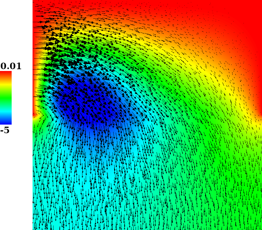
(a) Velocity.

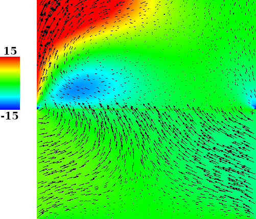
(b) Stresses.

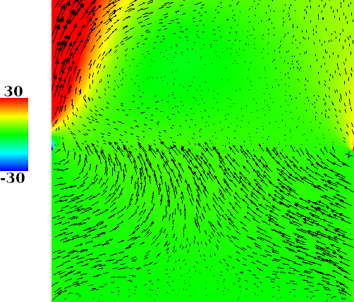
(c) Stresses.

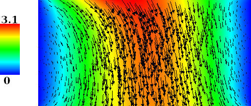
(d) Displacement.

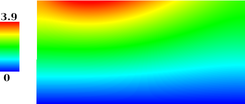
(e) Pore pressure.

Figure 1. Test case from section 6.3 with parameter set 1, $(\kappa,c_{0},\lambda,\mu^{b})=(1,1,1,1)$. Top left: $u^{s}$ and $z+\partial_{t}u^{b}$ (arrows) and $u^{s}_{2}$ and $z_{2}+\partial_{t}u^{b}_{2}$ (color). Top middle: $-(\sigma^{s}_{12},\sigma_{22}^{s})^{T}$ and $-(\sigma^{b}_{12},\sigma_{22}^{b})^{T}$ (arrows) and $-\sigma_{12}^{s}$ and $-\sigma_{12}^{b}$ (color). Top right: $-(\sigma^{s}_{12},\sigma_{22}^{s})^{T}$ and $-(\sigma^{b}_{12},\sigma_{22}^{b})^{T}$ (arrows) and $-\sigma_{22}^{s}$ and $-\sigma_{22}^{b}$ (color). Bottom left: $u^{b}$ (arrows) and $|u^{b}|$ (color). Bottom right: $p^{p}$.

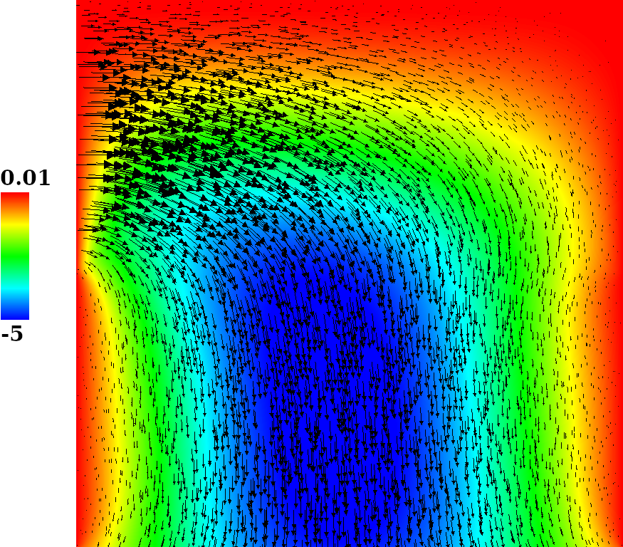
(a) Velocity.

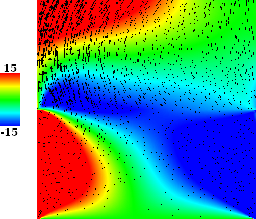
(b) Stresses.

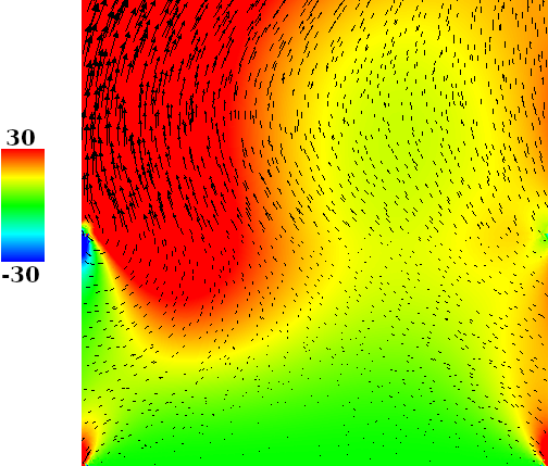
(c) Stresses.

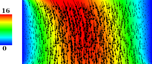
(d) Displacement.

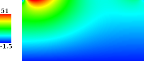
(e) Pore pressure.

Figure 2. Test case from section 6.3 with parameter set 2, $(\kappa,c_{0},\lambda,\mu^{b})=(10^{-4},10^{-4},10^{6},1)$. Top left: $u^{s}$ and $z+\partial_{t}u^{b}$ (arrows) and $u^{s}_{2}$ and $z_{2}+\partial_{t}u^{b}_{2}$ (color). Top middle: $-(\sigma^{s}_{12},\sigma_{22}^{s})^{T}$ and $-(\sigma^{b}_{12},\sigma_{22}^{b})^{T}$ (arrows) and $-\sigma_{12}^{s}$ and $-\sigma_{12}^{b}$ (color). Top right: $-(\sigma^{s}_{12},\sigma_{22}^{s})^{T}$ and $-(\sigma^{b}_{12},\sigma_{22}^{b})^{T}$ (arrows) and $-\sigma_{22}^{s}$ and $-\sigma_{22}^{b}$ (color). Bottom left: $u^{b}$ (arrows) and $|u^{b}|$ (color). Bottom right: $p^{p}$.

(a) Velocity.

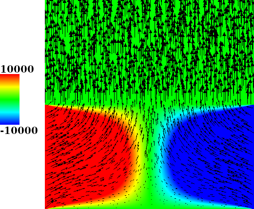
(b) Stresses.

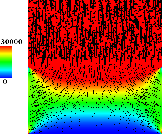
(c) Stresses.

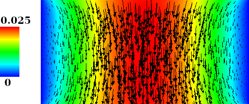
(d) Displacement.

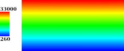
(e) Pore pressure.

Figure 3. Test case from section 6.3 with parameter set 3, $(\kappa,c_{0},\lambda,\mu^{b})=(10^{-4},10^{-4},10^{6},10^{6})$. Top left: $u^{s}$ and $z+\partial_{t}u^{b}$ (arrows) and $u^{s}_{2}$ and $z_{2}+\partial_{t}u^{b}_{2}$ (color). Top middle: $-(\sigma^{s}_{12},\sigma_{22}^{s})^{T}$ and $-(\sigma^{b}_{12},\sigma_{22}^{b})^{T}$ (arrows) and $-\sigma_{12}^{s}$ and $-\sigma_{12}^{b}$ (color). Top right: $-(\sigma^{s}_{12},\sigma_{22}^{s})^{T}$ and $-(\sigma^{b}_{12},\sigma_{22}^{b})^{T}$ (arrows) and $-\sigma_{22}^{s}$ and $-\sigma_{22}^{b}$ (color). Bottom left: $u^{b}$ (arrows) and $|u^{b}|$ (color). Bottom right: $p^{p}$.

7. Conclusions

We introduced an HDG method for the coupled Stokes–Biot problem that is provably robust in the incompressible limit, $\lambda\to\infty$ and $c_{0}\to 0$. Consistency was shown for the semi-discrete case while well-posedness and a priori error estimates were determined after combining the HDG method with backward Euler time-stepping. Furthermore, we showed that the discrete velocities and displacement are $H(\text{div})$-conforming and that the compressibility equations are satisfied pointwise by the numerical solution on the elements. Mass is conserved pointwise on the elements for the semi-discrete problem (up to the error of the $L^{2}$-projection of the source/sink term into the discrete pore pressure space). Finally, numerical examples demonstrate optimal rates of convergence for all unknowns in the $L^{2}$-norm and that the numerical method is locking-free.

Acknowledgements

Aycil Cesmelioglu and Jeonghun J. Lee gratefully acknowledge support by the National Science Foundation (grant numbers DMS-2110782 and DMS-2110781) and Sander Rhebergen gratefully acknowledges support from the Natural Sciences and Engineering Research Council of Canada through the Discovery Grant program (RGPIN-05606-2015).

Appendix A Proof of the inf-sup condition eq. 18

The inf-sup condition was proven for the case of homogeneous Dirichlet boundary conditions on the whole boundary of the domain in [34, Lemma 4.4] and [36, Lemma 1] for the HDG method and [37, Lemma 8] for a variation of the HDG method. Here we generalize these proofs to the case where homogeneous Dirichlet boundary conditions are only posed on part of the domain boundary. The proof proceeds in three steps.

Step 1. Let $\Pi_{V}^{j}\mathrel{\mathop{\mathchar 58\relax}}[H^{1}(\Omega^{j})]^{d}\to V_{h}^{j}$ be the BDM interpolation operator [12, Section III.3] and define the norm $\mathinner{\lVert v_{h}^{j}\rVert}_{1,h,j}$ as

$$\mathinner{\lVert v_{h}^{j}\rVert}_{1,h,j}^{2}\mathrel{\mathop{\mathchar 58\relax}}=\mathinner{\lVert\varepsilon(v_{h}^{j})\rVert}_{\Omega^{j}}^{2}+\sum_{F\in\mathcal{F}^{j}}h_{F}^{-1}\mathinner{\lVert\llbracket v_{h}^{j}\rrbracket\rVert}_{F}^{2},$$

where $h_{F}$ is the radius of the face $F$. Note that

$$\mathopen{|\mkern-1.5mu|\mkern-1.5mu|}(v_{h},\{\!\!\{v_{h}\}\!\!\})\mathclose{|\mkern-1.5mu|\mkern-1.5mu|}_{v,j}^{2}=\sum_{K\in\mathcal{T}^{j}}\mathinner{\bigl{(}\mathinner{\lVert\varepsilon(v_{h})\rVert}_{K}^{2}+h_{K}^{-1}\mathinner{\lVert v_{h}-\{\!\!\{v_{h}\}\!\!\}\rVert}_{\partial K}^{2}\bigr{)}}.$$

On boundary facets $\{\!\!\{v_{h}\}\!\!\}=v_{h}$ and so

$$\begin{split}\sum_{K\in\mathcal{T}^{j}}h_{K}^{-1}\mathinner{\lVert(v_{h}-\{\!\!\{v_{h}\}\!\!\})\rVert}_{\partial K}^{2}=&\sum_{F\in\mathcal{F}^{j}_{int}}\mathinner{\bigl{(}h_{K^{+}}^{-1}\mathinner{\lVert(v_{h}^{+}-\{\!\!\{v_{h}\}\!\!\})\rVert}_{F}^{2}+h_{K^{-}}^{-1}\mathinner{\lVert(v_{h}^{-}-\{\!\!\{v_{h}\}\!\!\})\rVert}_{F}^{2}\bigr{)}}\\ =&\sum_{F\in\mathcal{F}^{j}_{int}}\mathinner{\bigl{(}\tfrac{1}{4}h_{K^{+}}^{-1}\mathinner{\lVert v_{h}^{+}-v_{h}^{-}\rVert}_{F}^{2}+\tfrac{1}{4}h_{K^{-}}^{-1}\mathinner{\lVert v_{h}^{-}-v_{h}^{+}\rVert}_{F}^{2}\bigr{)}}\\ =&\sum_{F\in\mathcal{F}^{j}_{int}}\tfrac{1}{4}\mathinner{(h_{K^{+}}^{-1}+h_{K^{-}}^{-1})}\mathinner{\lVert v_{h}^{+}-v_{h}^{-}\rVert}_{F}^{2}\\ \leq&C\sum_{F\in\mathcal{F}^{j}_{int}}h_{F}^{-1}\mathinner{\lVert\llbracket v_{h}\rrbracket\rVert}_{F}^{2},\end{split}$$

where, assuming shape regularity of the mesh, the inequality is by equivalence of $h_{F}$, $h_{K^{+}}$, and $h_{K^{-}}$ where $F$ is a facet shared by $K^{+}$ and $K^{-}$. Throughout this proof $C>0$ is a generic constant independent of $h$. This shows that $\mathopen{|\mkern-1.5mu|\mkern-1.5mu|}(v_{h},\{\!\!\{v_{h}\}\!\!\})\mathclose{|\mkern-1.5mu|\mkern-1.5mu|}_{v,j}\leq C\mathinner{\lVert v_{h}^{j}\rVert}_{1,h,j}$. Then, for all $v\in[H^{1}(\Omega^{j})]^{d}$,

(61) $$\mathopen{|\mkern-1.5mu|\mkern-1.5mu|}(\Pi_{V}^{j}v,\{\!\!\{\Pi_{V}^{j}v\}\!\!\})\mathclose{|\mkern-1.5mu|\mkern-1.5mu|}_{v,j}\leq C\mathinner{\lVert\Pi_{V}^{j}v\rVert}_{1,h,j}\leq C\mathinner{\lVert v\rVert}_{1,\Omega^{j}}^{2},$$

where the second inequality was shown in the proof of [24, Proposition 10]. We next define

$$\begin{split}[H^{1}_{ID,j}(\Omega^{j})]^{d}&\mathrel{\mathop{\mathchar 58\relax}}=\mathinner{\bigl{\{}v\in[H^{1}(\Omega^{j})]^{d}\ \mathrel{\mathop{\mathchar 58\relax}}\ v=0\text{ on }\Gamma_{I}\cup\Gamma_{D}^{j}\bigr{\}}},\\ \tilde{\tilde{\boldsymbol{V}}}_{h}^{j}&\mathrel{\mathop{\mathchar 58\relax}}=\mathinner{\bigl{\{}\boldsymbol{v}_{h}\in\widetilde{\boldsymbol{V}}_{h}^{j}\ \mathrel{\mathop{\mathchar 58\relax}}\ v_{h}\in H(\text{div};\Omega^{j}),\ \bar{v}_{h}^{j}\cdot n=v_{h}^{j}\cdot n\text{ on }\partial\Omega^{j}\bigr{\}}}.\end{split}$$

Given $|\Gamma_{N}^{j}|>0$, it was shown in [5, Lemma B.1] that there exists a constant $C>0$ such that for all $q_{h}\in Q_{h}^{j}$ there is a $v_{q_{h}}\in[H^{1}_{ID,j}(\Omega^{j})]^{d}$ that satisfies

(62) $$-\nabla\cdot v_{q_{h}}=q_{h}\qquad C\mathinner{\lVert v_{q_{h}}\rVert}_{1,\Omega^{j}}\leq\mathinner{\!\left\lVert q_{h}\right\rVert}_{\Omega^{j}}.$$

By eqs. 61 and 62 we note that

$$\mathopen{|\mkern-1.5mu|\mkern-1.5mu|}(\Pi_{V}^{j}v_{q_{h}},\{\!\!\{\Pi_{V}^{j}v_{q_{h}}\}\!\!\})\mathclose{|\mkern-1.5mu|\mkern-1.5mu|}_{v,j}\leq C\mathinner{\lVert v_{q_{h}}\rVert}_{1,\Omega^{j}}\leq C\mathinner{\!\left\lVert q_{h}\right\rVert}_{\Omega^{j}}.$$

Note also that $(\Pi_{V}^{j}v_{q_{h}},\{\!\!\{\Pi_{V}^{j}v_{q_{h}}\}\!\!\})\in\tilde{\tilde{\boldsymbol{V}}}_{h}^{j}$. We therefore find that

$$\sup_{0\neq\boldsymbol{v}_{h}\in\tilde{\tilde{\boldsymbol{V}}}_{h}^{j}}\frac{b_{h}^{j}((q_{h}^{j},0),\boldsymbol{v}_{h})}{\mathopen{|\mkern-1.5mu|\mkern-1.5mu|}\boldsymbol{v}_{h}\mathclose{|\mkern-1.5mu|\mkern-1.5mu|}_{v,j}}\geq\frac{b_{h}^{j}((q_{h}^{j},0),(\Pi_{V}^{j}v_{q_{h}},\{\!\!\{\Pi_{V}^{j}v_{q_{h}}\}\!\!\}))}{\mathopen{|\mkern-1.5mu|\mkern-1.5mu|}(\Pi_{V}^{j}v_{q_{h}},\{\!\!\{\Pi_{V}^{j}v_{q_{h}}\}\!\!\})\mathclose{|\mkern-1.5mu|\mkern-1.5mu|}_{v,j}}\geq C\mathinner{\lVert q_{h}^{j}\rVert}_{\Omega^{j}}.$$

Step 2. Noting that $(v_{h},0)\in\widetilde{\boldsymbol{V}}_{h}^{j}$, there exists a $C$ such that

(63) $$\sup_{\boldsymbol{0}\neq\boldsymbol{v}_{h}\in\widetilde{\boldsymbol{V}}_{h}^{j}}\frac{b_{h}^{j}((0,\bar{q}_{h}),\boldsymbol{v}_{h})}{\mathopen{|\mkern-1.5mu|\mkern-1.5mu|}\boldsymbol{v}_{h}\mathclose{|\mkern-1.5mu|\mkern-1.5mu|}_{v,j}}\geq\sup_{0\neq v_{h}\in V_{h}^{j}}\frac{b_{h}^{j}((0,\bar{q}_{h}),(v_{h},0))}{\mathopen{|\mkern-1.5mu|\mkern-1.5mu|}(v_{h},0)\mathclose{|\mkern-1.5mu|\mkern-1.5mu|}_{v,j}}\geq C\mathopen{|\mkern-1.5mu|\mkern-1.5mu|}(0,\bar{q}_{h})\mathclose{|\mkern-1.5mu|\mkern-1.5mu|}_{q,j}\quad\forall\bar{q}_{h}\in\bar{Q}_{h}^{j},$$

where the second inequality was shown in the proof of [36, Lemma 3]. (Although [36, Lemma 3] assumed quasi-conformity, the result can be extended to shape-regular meshes.)

Step 3. Define $b_{1}^{j}((q_{h}^{j},0),\boldsymbol{v}_{h})=b_{h}^{j}((q_{h}^{j},0),\boldsymbol{v}_{h})$ and $b_{2}^{j}((0,\bar{q}_{h}),\boldsymbol{v}_{h})=b_{h}^{j}((0,\bar{q}_{h}),\boldsymbol{v}_{h})$. Noting that

$$\tilde{\tilde{\boldsymbol{V}}}_{h}^{j}=\mathinner{\bigl{\{}\boldsymbol{v}_{h}\in\widetilde{\boldsymbol{V}}_{h}^{j}\ \mathrel{\mathop{\mathchar 58\relax}}\ b_{2}^{j}((0,\bar{q}_{h}),\boldsymbol{v}_{h})=0\ \forall\bar{q}_{h}\in\bar{Q}_{h}^{j}\bigr{\}}},$$

the result follows after applying [25, Theorem 3.1].

Appendix B Proof of the inf-sup condition eq. 19

The proof is similar to that given in appendix A. It is given here for completeness. The proof again proceeds in three steps.

Step 1. Let $\Pi_{V}\mathrel{\mathop{\mathchar 58\relax}}[H^{1}(\Omega)]^{d}\to V_{h}$ be the BDM interpolation operator [12, Section III.3] and define the norm $\mathinner{\lVert v_{h}\rVert}_{1,h}$ as

$$\mathinner{\lVert v_{h}\rVert}_{1,h}^{2}\mathrel{\mathop{\mathchar 58\relax}}=\mathinner{\lVert\varepsilon(v_{h})\rVert}_{\Omega}^{2}+\sum_{F\in\mathcal{F}}h_{F}^{-1}\mathinner{\lVert\llbracket v_{h}\rrbracket\rVert}_{F}^{2},$$

where $h_{F}$ is the radius of the face $F$. As in appendix A we have that for all $v\in[H^{1}(\Omega)]^{d}$,

(64) $$\mathopen{|\mkern-1.5mu|\mkern-1.5mu|}(\Pi_{V}v,\{\!\!\{\Pi_{V}v\}\!\!\},\{\!\!\{\Pi_{V}v\}\!\!\})\mathclose{|\mkern-1.5mu|\mkern-1.5mu|}_{v}\leq C\mathinner{\lVert\Pi_{V}v\rVert}_{1,h}\leq C\mathinner{\lVert v\rVert}_{1,\Omega},$$

where, in this proof, $C>0$ is a generic constant independent of $h$. Let $\Gamma_{D}=\Gamma_{D}^{s}\cup\Gamma_{D}^{b}$ and $\Gamma_{N}=\Gamma_{N}^{s}\cup\Gamma_{N}^{b}$ and define

$$\begin{split}[H^{1}_{D}(\Omega)]^{d}&\mathrel{\mathop{\mathchar 58\relax}}=\mathinner{\bigl{\{}v\in[H^{1}(\Omega)]^{d}\ \mathrel{\mathop{\mathchar 58\relax}}\ v=0\text{ on }\Gamma_{D}\bigr{\}}},\\ \tilde{\tilde{\boldsymbol{V}}}_{h}&\mathrel{\mathop{\mathchar 58\relax}}=\mathinner{\bigl{\{}\boldsymbol{v}_{h}\in\widehat{\boldsymbol{V}}_{h}\ \mathrel{\mathop{\mathchar 58\relax}}\ v_{h}\in H(\text{div};\Omega),\ \bar{v}_{h}^{s}\cdot n=\bar{v}_{h}^{b}\cdot n=v_{h}\cdot n\text{ on }\partial\Omega\cup\Gamma_{I}\bigr{\}}}.\end{split}$$

Given $|\Gamma_{N}|>0$ there exists a constant $C>0$ such that for all $q_{h}\in Q_{h}$ there is a $v_{q_{h}}\in[H^{1}_{D}(\Omega)]^{d}$ that satisfies (see [5, Lemma B.1])

(65) $$-\nabla\cdot v_{q_{h}}=q_{h}\qquad C\mathinner{\lVert v_{q_{h}}\rVert}_{1,\Omega}\leq\mathinner{\!\left\lVert q_{h}\right\rVert}_{\Omega}.$$

By eqs. 64 and 65,

$$\mathopen{|\mkern-1.5mu|\mkern-1.5mu|}(\Pi_{V}v_{q_{h}},\{\!\!\{\Pi_{V}v_{q_{h}}\}\!\!\},\{\!\!\{\Pi_{V}v_{q_{h}}\}\!\!\})\mathclose{|\mkern-1.5mu|\mkern-1.5mu|}_{v}\leq C\mathinner{\lVert v_{q_{h}}\rVert}_{1,\Omega}\leq C\mathinner{\!\left\lVert q_{h}\right\rVert}_{\Omega}.$$

Since $(\Pi_{V}v_{q_{h}},\{\!\!\{\Pi_{V}v_{q_{h}}\}\!\!\},\{\!\!\{\Pi_{V}v_{q_{h}}\}\!\!\})\in\tilde{\tilde{\boldsymbol{V}}}_{h}$ we obtain

$$\sup_{0\neq\boldsymbol{v}_{h}\in\tilde{\tilde{\boldsymbol{V}}}_{h}}\frac{b_{h}((q_{h},0),\boldsymbol{v}_{h})}{\mathopen{|\mkern-1.5mu|\mkern-1.5mu|}\boldsymbol{v}_{h}\mathclose{|\mkern-1.5mu|\mkern-1.5mu|}_{v}}\geq\frac{b_{h}((q_{h},0),(\Pi_{V}v_{q_{h}},\{\!\!\{\Pi_{V}v_{q_{h}}\}\!\!\},\{\!\!\{\Pi_{V}v_{q_{h}}\}\!\!\}))}{\mathopen{|\mkern-1.5mu|\mkern-1.5mu|}(\Pi_{V}v_{q_{h}},\{\!\!\{\Pi_{V}v_{q_{h}}\}\!\!\},\{\!\!\{\Pi_{V}v_{q_{h}}\}\!\!\})\mathclose{|\mkern-1.5mu|\mkern-1.5mu|}_{v}}\geq C\mathinner{\lVert q_{h}\rVert}_{\Omega}.$$

Step 2. Noting that $(v_{h},0,0)\in\widehat{\boldsymbol{V}}_{h}$, there exists a $C$ such that

(66) $$\sup_{\boldsymbol{0}\neq\boldsymbol{v}_{h}\in\widehat{\boldsymbol{V}}_{h}}\frac{b_{h}((0,\bar{q}_{h}),\boldsymbol{v}_{h})}{\mathopen{|\mkern-1.5mu|\mkern-1.5mu|}\boldsymbol{v}_{h}\mathclose{|\mkern-1.5mu|\mkern-1.5mu|}_{v}}\geq\sup_{0\neq v_{h}\in V_{h}}\frac{b_{h}((0,\bar{q}_{h}),(v_{h},0,0))}{\mathopen{|\mkern-1.5mu|\mkern-1.5mu|}(v_{h},0,0)\mathclose{|\mkern-1.5mu|\mkern-1.5mu|}_{v}}\geq C\mathopen{|\mkern-1.5mu|\mkern-1.5mu|}(0,\bar{q}_{h})\mathclose{|\mkern-1.5mu|\mkern-1.5mu|}_{q}\quad\forall\bar{q}_{h}\in\bar{Q}_{h},$$

where the second inequality was shown in the proof of [36, Lemma 3].

Step 3. Define $b_{1}((q_{h},0),\boldsymbol{v}_{h})=b_{h}((q_{h},0),\boldsymbol{v}_{h})$ and $b_{2}((0,\bar{q}_{h}),\boldsymbol{v}_{h})=b_{h}((0,\bar{q}_{h}),\boldsymbol{v}_{h})$. Noting that

$$\begin{split}\tilde{\tilde{\boldsymbol{V}}}_{h}&=\mathinner{\bigl{\{}\boldsymbol{v}_{h}\in\widehat{\boldsymbol{V}}_{h}\ \mathrel{\mathop{\mathchar 58\relax}}\ v_{h}^{j}\in H(\text{div};\Omega^{j}),\ \bar{v}_{h}^{j}\cdot n=v_{h}^{j}\cdot n\text{ on }\partial\Omega\cup\Gamma_{I},\ j=s,b\bigr{\}}}.\\ &=\mathinner{\bigl{\{}\boldsymbol{v}_{h}\in\widehat{\boldsymbol{V}}_{h}\ \mathrel{\mathop{\mathchar 58\relax}}\ b_{2}((0,\bar{q}_{h}),\boldsymbol{v}_{h})=0\ \forall\bar{q}_{h}\in\bar{Q}_{h}\bigr{\}}},\end{split}$$

the result follows after applying [25, Theorem 3.1].

References

- [1] Ilona Ambartsumyan, Vincent J. Ervin, Truong Nguyen, and Ivan Yotov. A nonlinear Stokes-Biot model for the interaction of a non-Newtonian fluid with poroelastic media. ESAIM Math. Model. Numer. Anal., 53(6):1915–1955, 2019.
- [2] Ilona Ambartsumyan, Eldar Khattatov, Ivan Yotov, and Paolo Zunino. A Lagrange multiplier method for a Stokes-Biot fluid-poroelastic structure interaction model. Numer. Math., 140(2):513–553, 2018.
- [3] D. N. Arnold, F. Brezzi, and M. Fortin. A stable finite element for the Stokes equations. Calcolo, 21(4):337–344 (1985), 1984.
- [4] S. Badia, A. Quaini, and A. Quarteroni. Coupling Biot and Navier-Stokes equations for modelling fluid-poroelastic media interaction. J. Comput. Phys., 228(21):7986–8014, 2009.
- [5] T. Bærland, J. J. Lee, K.-A. Mardal, and R. Winther. Weakly imposed symmetry and robust preconditioners for Biot’s consolidation model. Computational Methods in Applied Mathematics, 17(3):377–396, 2017.
- [6] G. S. Beavers and D. D. Joseph. Boundary conditions at a naturally impermeable wall. J. Fluid. Mech, 30(1):197–207, 1967.
- [7] E. A. Bergkamp, C. V. Verhoosel, J. J. C. Remmers, and D. M. J. Smeulders. A staggered finite element procedure for the coupled Stokes-Biot system with fluid entry resistance. Comput. Geosci., 24(4):1497–1522, 2020.
- [8] M. A. Biot. General theory of three-dimensional consolidation. Journal of applied physics, 12(2):155–164, 1941.
- [9] M. A. Biot. Theory of elasticity and consolidation for a porous anisotropic solid. J. Appl. Phys., 26:182–185, 1955.
- [10] M. A. Biot and D. G. Willis. The elastic coefficients of the theory of consolidation. J. Appl. Mech., 24:594–601, 1957.
- [11] S. C. Brenner. Poincaré-Friedrichs inequalities for piecewise functions. SIAM J. Numer. Anal., 41(1):306–324, 2003.
- [12] F. Brezzi and M. Fortin. Mixed and Hybrid Finite Element Methods, volume 15 of Springer Series in Computational Mathematics. Springer–Verlag New York Inc., 1991.
- [13] Franco Brezzi, Jim Douglas, Jr., and L. D. Marini. Two families of mixed finite elements for second order elliptic problems. Numer. Math., 47(2):217–235, 1985.
- [14] A. Buffa and C. Ortner. Compact embeddings of broken Sobolev spaces and applications. IMA J. Numer. Anal., 29(4):827–855, 2009.
- [15] M. Bukač. A loosely-coupled scheme for the interaction between a fluid, elastic structure and poroelastic material. J. Comput. Phys., 313:377–399, 2016.
- [16] M. Bukač, I. Yotov, R. Zakerzadeh, and P. Zunino. Partitioning strategies for the interaction of a fluid with a poroelastic material based on a Nitsche’s coupling approach. Comput. Methods Appl. Mech. Engrg., 292:138–170, 2015.
- [17] A. Cesmelioglu. Analysis of the coupled Navier-Stokes/Biot problem. J. Math. Anal. Appl., 456(2):970–991, 2017.
- [18] A. Cesmelioglu and P. Chidyagwai. Numerical analysis of the coupling of free fluid with a poroelastic material. Numer. Methods Partial Differential Equations, 36(3):463–494, 2020.
- [19] A. Cesmelioglu, J. J. Lee, and S. Rhebergen. Analysis of an embedded–hybridizable discontinuous Galerkin method for Biot’s consolidation model. Submitted, 2022.
- [20] A. Cesmelioglu, S. Rhebergen, and G. N. Wells. An embedded–hybridized discontinuous Galerkin method for the coupled Stokes–Darcy system. Journal of Computational and Applied Mathematics, 367:112476, 2020.
- [21] B. Cockburn, J. Gopalakrishnan, and R. Lazarov. Unified hybridization of discontinuous Galerkin, mixed, and continuous Galerkin methods for second order elliptic problems. SIAM J. Numer. Anal., 47(2):1319–1365, 2009.
- [22] G. Fu and C. Lehrenfeld. A strongly conservative hybrid DG/mixed FEM for the coupling of Stokes and Darcy flow. J. Sci. Comput., 2018.
- [23] Vivette Girault and Pierre-Arnaud Raviart. Finite element methods for Navier-Stokes equations, volume 5 of Springer Series in Computational Mathematics. Springer-Verlag, Berlin, 1986. Theory and algorithms.
- [24] P. Hansbo and M. G. Larson. Discontinuous Galerkin methods for incompressible and nearly incompressible elasticity by Nitsche’s method. Comput. Methods Appl. Mech. Engrg., 191:1895–1908, 2002.
- [25] J. S. Howell and N. J. Walkington. Inf-sup conditions for twofold saddle point problems. Numer. Math., 118:663–693, 2011.
- [26] G. Kanschat and B. Rivière. A strongly conservative finite element method for the coupling of Stokes and Darcy flow. J. Comput. Phys., 229(17):5933–5943, 2010.
- [27] J. J. Lee, K. Mardal, and R. Winther. Parameter-robust discretization and preconditioning of Biot’s consolidation model. SIAM Journal on Scientific Computing, 39(1):A1–A24, 2017.
- [28] Jeonghun J. Lee. Robust error analysis of coupled mixed methods for Biot’s consolidation model. J. Sci. Comput., 69(2):610–632, 2016.
- [29] Tongtong Li and Ivan Yotov. A mixed elasticity formulation for fluid-poroelastic structure interaction. ESAIM Math. Model. Numer. Anal., 56(1):1–40, 2022.
- [30] C. Lovadina and R. Stenberg. Energy norm a posteriori error estimates for mixed finite element methods. Math. Comp., 75(256):1659–1674, 2006.
- [31] R. Oyarzúa and R. Ruiz-Baier. Locking-free finite element methods for poroelasticity. SIAM J. Numer. Anal., 54(5):2951–2973, 2016.
- [32] Oyekola Oyekole and Martina Bukač. Second-order, loosely coupled methods for fluid-poroelastic material interaction. Numer. Methods Partial Differential Equations, 36(4):800–822, 2020.
- [33] P.-A. Raviart and J. M. Thomas. A mixed finite element method for 2nd order elliptic problems. In Mathematical aspects of finite element methods (Proc. Conf., Consiglio Naz. delle Ricerche (C.N.R.), Rome, 1975), pages 292–315. Lecture Notes in Math., Vol. 606, 1977.
- [34] S. Rhebergen and G. N. Wells. Analysis of a hybridized/interface stabilized finite element method for the Stokes equations. SIAM J. Numer. Anal., 55(4):1982–2003, 2017.
- [35] S. Rhebergen and G. N. Wells. A hybridizable discontinuous Galerkin method for the Navier–Stokes equations with pointwise divergence-free velocity field. J. Sci. Comput., 76(3):1484–1501, 2018.
- [36] S. Rhebergen and G. N. Wells. Preconditioning of a hybridized discontinuous Galerkin finite element method for the Stokes equations. J. Sci. Comput., 77(3):1936–1952, 2018.
- [37] S. Rhebergen and G. N. Wells. An embedded–hybridized discontinuous Galerkin finite element method for the Stokes equations. Comput. Methods Appl. Mech. Engrg., 358:112619, 2020.
- [38] R. Ruiz-Baier, M. Taffetani, H. D. Westermeyer, and I. Yotov. The Biot–Stokes coupling using total pressure: Formulation, analysis and application to interfacial flow in the eye. Computer Methods in Applied Mechanics and Engineering, 389:114384, 2022.
- [39] P. Saffman. On the boundary condition at the surface of a porous media. Stud. Appl. Math., 50:292–315, 1971.
- [40] J. Schöberl. An advancing front 2D/3D-mesh generator based on abstract rules. J. Comput. Visual Sci., 1(1):41–52, 1997.
- [41] J. Schöberl. C++11 implementation of finite elements in NGSolve. Technical Report ASC Report 30/2014, Institute for Analysis and Scientific Computing, Vienna University of Technology, 2014.
- [42] Ralph E. Showalter. Poroelastic filtration coupled to Stokes flow. In Control theory of partial differential equations, volume 242 of Lect. Notes Pure Appl. Math., pages 229–241. Chapman & Hall/CRC, Boca Raton, FL, 2005.
- [43] C. Taylor and P. Hood. A numerical solution of the Navier-Stokes equations using the finite element technique. Internat. J. Comput. & Fluids, 1(1):73–100, 1973.