neutrino-induced single pion production and the reanalyzed bubble chamber data

Abstract

In this work we report the calculation of the charged current total and differential cross sections for weak pion-production with neutrinos and antineutrinos, with the final pion-nucleon pair invariant mass $W_{\pi N}\lesssim 2$GeV. Our results are compared with the recent reanalyzed data from the old bubble chamber experiments, that solved the discrepancy between the ANL and BNL data. We implement a model previously tested for the cuts $W_{\pi N}<1.4,1.6$ Gev which includes explicitly resonances in the first and second resonance regions, within different approaches for the resonances self energy and $\frac{3}{2}$-vertexes and propagators, a fact not usually analyzed. Our model leans on consistent effective Lagrangians that generate resonant amplitudes together non resonant plus resonant backgrounds. Effects of hadrons finite extension and more energetic resonances corresponding to the emitted pion-nucleon invariant mass in the $1.6<W_{\pi N}<2$ GeV region, are taking into account using appropiate form factors in consistency with previous results on neutral current pion production calculations. Our results reproduce well the reanalysed data without cuts and are compared with another models.

PACS numbers :13.15.+g,13.75.-n,13.60.Le

I INTRODUCTION

For current and future neutrino oscillation experiments we need to understand single pion production by neutrinos with few-GeV energies. The pion production is either a signal process when scattering cross sections are analyzed, or a large background for analyses which select quasielastic events. At these energies the dominant production mechanism is via the excitation and subsequent decay of hadronic resonances. Experimental data on nuclear targets present a confusing picture, shown from the MINERνA Eberly15 (1, 2)and MiniBooNE Are11 (3) experiments in poor agreement with each other in the framework of current theoretical modelsSob15 (4, 5). Complete models of neutrino–nucleus single pion production interactions are usually factorized into three parts: the neutrino–nucleon cross section; additional nuclear effects which affect the initial interaction; and the “final state interactions” (FSI) of hadrons exiting the nucleus.

More basically at the level of neutrino-nucleon cross section, the axial form factor(FF) for pion production on free nucleons cannot be constrained by electron scattering data, used normally to get the vector FF, so it relies upon data from Argonne National Laboratory’s 12 ft bubble chamber (ANL)Rad82 (6) and Brookhaven National Laboratory’s 7 ft bubble chamber (BNL)Kitagi86 (7). The ANL neutrino beam was produced by focusing 12.4 GeV protons onto a beryllium target. Two magnetic horns were used to focus the positive pions produced by the primary beam in the direction of the bubble chamber, these secondary particles decayed to produce a predominantly $\nu_{\mu}$ peaked at $\sim 0.5$ GeV. The BNL neutrino beam was produced by focusing 29 GeV protons on a sapphire target, with a similar two horn design to focus the secondary particles. The BNL $\nu_{\mu}$ beam had a higher peak energy of $\sim 1.2$ GeV, and was broader than the ANL one. These both datasets differed in normalization by 30–40$\%$ for the leading pion production process $\nu_{\mu}p\rightarrow\mu^{-}p\pi^{+}$, which conduced to large uncertainties in the predictions for oscillation experiments as well as in the interpretation of data taken on nuclear targetsNieves07 (8, 9, 12, 10, 13, 14).

It has long been suspected that the discrepancy between ANL and BNL was due to an issue with the normalization of the flux prediction from one or both experiments, and it has been shown by other authors that their published results are consistent within the experimental uncertainties providedGraczyk09 (15, 16). In Ref. wilki14 (17), was presented a method for removing flux normalization uncertainties from the ANL and BNL $\nu_{\mu}p\rightarrow\mu^{-}p\pi^{+}$ measurements by taking ratios with charged-current quasielastic (CCQE) event rates in which the normalization cancels. Then, it was obtained a measurement of $\nu_{\mu}p\rightarrow\mu^{-}p\pi^{+}$by multiplying the ratio by an independent measurement of the charged quasielastic (CCQE) cross section which is well known for nucleon targets. Using this technique, they found good agreement between the ANL and BNL $\nu_{\mu}p\rightarrow\mu^{-}p\pi^{+}$datasets. Later, they extend that method to include the subdominant $\nu_{\mu}n\rightarrow\mu^{-}p\pi^{0}$ and $\nu_{\mu}n\rightarrow\mu^{-}n\pi^{+}$channelsRodriguez16 (18). These authors used the resulting data to fit the parameters of the GENIE pion production modelGenie10 (19). They found a set of parameters that can describe the bubble chamber data better than the GENIE default ones, and provided updated central values and reduced uncertainties for use in neutrino oscillation and cross section analyses which use the GENIE model. In this model the cross section is cutted off at a tunable invariant mass value, which is $W_{\pi N}\leq 1.7$ GeV by default. No in-medium modifications to resonances are considered, and interferences between resonances are neglected in the calculation being the Rein–Sehgal(RS) model in Ref.Rein81 (20) adopted. Nevertheless, the original RS model includes non-resonant single pion production as an additional resonance amplitude, while in GENIE the non-resonant component is implemented as an extension of the deep inelastic scattering model. They found that GENIE’s non-resonant background prediction has to be significantly reduced to fit the data, which may help to explain the recent discrepancies between simulation and data observed by the MINERνA coherent pion and NOνAAdanson2016 (21) oscillation analyses.While more sophisticated single pion production models exist, the GENIE generator is widely used by current and planned neutrino oscillation experiments, so tuning the generator parameters represents a pragmatic approach to improving its description of available data. We find that the reanalyzed data, where the normalization discrepancy has been resolved, is able to significantly reduce the uncertainties on the pion production parameters.

This is one of the reasons encourage us to return to the calculation of neutrino-nucleon cross sections in our model and try to extend it to larger final $W_{\pi N}$ invariant masses. On the other hand, there are many models to describe this process that do not fulfill several important ingredients:
i)There are problems from the formal point of view. The main pion emision source are excitation and decay of resonances, and many of them are of spin $\frac{3}{2}$ where its field is built as $\Psi_{\mu}\equiv\psi\otimes\xi_{\mu}$, where $\psi$ is a Dirac spinor field and $\xi_{\mu}$ is a Dirac 4-vector Kirbach2002 (22). In this way, the field $\Psi_{\mu}$ will contain a physical spin-$\frac{3}{2}$ sector and a spurious spin-$\frac{1}{2}$ sector dragged by construction. Nevertheless, involved Lagrangians must lead to amplitudes invariant by contact transformationsBadagnani12 (23)$\Psi^{\nu}\rightarrow\Psi^{{}^{\prime}\nu}=R_{\mu\nu}(\frac{1+3A}{2})\Psi^{\nu},R^{\rho\sigma}(a)=g^{\rho\sigma}+a\gamma^{\rho}\gamma^{\sigma}$, which change the amount of the spin-$\frac{1}{2}$ espurious contribution since there exist the constraint $\Psi_{\mu}\gamma^{\mu}=0$ for the $\frac{3}{2}$ sector. Many works keep the simpler forms of both the free and interaction Lagrangians involving $\Psi_{\mu}$, that correspond to different $A$ values, and with this choice amplitudes lacks the mentioned invariance. In addition, the interaction Lagrangian for the spin-$\frac{3}{2}$ field coupled to a nucleon N ($\psi$) and a pseudo-scalar meson ($\phi$) or boson ($W$), as usually appears in a resonance production-decay, depends on a second parameter $Z$ not fixed by the contact invariance. Now to fix it, we point to the question of the true degree of freedom of the spin-$\frac{3}{2}$ field, which dynamics is described by a constrained quantum field theory. Observe that in the free $\Psi_{\mu}$ Lagrangian there is no term containing $\dot{\Psi}_{0}$ Badga17 (24). So, the equation of motion for it is a true constraint, and $\Psi_{0}$ should have no dynamics. It is necessary then that interactions do not change that fact and as was shown in Ref. Badga17 (24) this is fulfilled for certain values of $Z$. These formal points are usually not analyzed in the majority of works on the field.
ii)In addition to the resonances pole or direct contribution (normaly referred as direct resonant or simply resonant, terms) to the amplitude, we have background terms coming from cross resonance amplitudes (named ussually background resonant terms) and non-resonance origin (called usually background non resonant terms). Many works do not consider the interference between these both resonant and background contributions and really it is very important to describe the data.
iii)Finally, another models detach the decay process from the resonance production out of the whole weak production amplitude. However, resonances are nonperturbative phenomena associated to the pole of the S-matrix amplitude and one cannot detach them from its production or decay mechanisms. Further, the models to describe cross sections use born contributions for the background amplitudes and resonant ones that are valid around each resonance region. Nevertheless, the effect of deviations from the hadronic pointlike couplings due to the quark structure of nucleons and resonances are not taken into account when the final $\pi N$ invariant mass $W_{\pi N}$ grows, and it is assumed that that models are valid for all $W_{\pi N}$ regions.

In this work we calculate the total and differential cross sections of the inelastic dispersion of neutrinos on nucleons with the production of one pion until $W_{\pi N}\lesssim 2$ GeV and we try to describe the reanalysed data in Refs.wilki14 (17, 18). In our model we incorporate explicitly resonance states $\Delta(1232)$, and $N^{*}(1440),N^{*}(1520),N^{*}(1535)$, the so called second resonance region, with a consistent model for the spin-$\frac{3}{2}$ fields that reproduced satisfactorily the data for the ANL experiment in the range $W_{\pi N}\lesssim 1.6$ GeV Tamayo22 (11). The effect of hadron structure when $W_{\pi N}$ grows and of more energetic resonances, not introduced explicitly in the model, is included throught a global effective hadronic FF in consistence with previous calculations for neutral currents(NC) Mariano11 (25). Our model reproduces well the data of Refs.wilki14 (17, 18), both for the total and differential cross sections.

Our work will be organized as follows: In Section II, we summaryze the general description of the pion production cross sections, together with the previously calculated amplitudes showed in the Appendix. In Section III we analyze how to extend our previous model to higher $W_{\pi N}$ and will show our results for neutrino and antineutrino scattering. Finally, in Section V we summaryze our conclusions.

II Total and differential cross sections

We resume here some general concepts and let specific formulae for an Appendix. We are interested in describing here two observables for the charged current (CC) $\nu N\rightarrow\mu^{+}N^{\prime}\pi$ and $\bar{\nu}N\rightarrow\mu^{-}N^{\prime}\pi$ modes, since neutral current (NC) processes in the present $W_{\pi N}$-range, where analyzed previously Mariano11 (25). The total cross section for single pion weak production on nucleons, where we use $\nu N$ center mass (CM) variables since it is easier to look for their limits, reads (we take $\boldsymbol{p}_{\nu}=E_{\nu}\hat{\boldsymbol{k}}$ along the z-axis)

$$\sigma(E_{{}_{\nu}}^{\text{CM}}) = \frac{m_{{}_{\nu}}m_{{}_{N}}^{2}}{(2\pi)^{4}E_{{}_{\nu}}^{\text{CM}}\sqrt{s}}\int\limits_{E_{\mu}^{{}^{-}}}^{E_{\mu}^{{}^{+}}}dE_{{}_{\mu}}^{\text{CM}}\int\limits_{E_{\pi}^{{}^{-}}}^{E_{\pi}^{{}^{+}}}dE_{{}_{\pi}}^{\text{CM}}\int\limits_{-1}^{+1}d\cos\theta\int\limits_{0}^{2\pi}d\eta\frac{1}{16}\sum\limits_{\text{spin}}|\mathcal{M}|^{2},$$ (1)

being $\sqrt{s}=E_{{}_{\nu}}^{\text{CM}}+E_{{}_{N}}^{\text{CM}}=\sqrt{2E_{{}_{\nu}}m_{{}_{N}}+m_{{}_{N}}^{2}}$, $d\Omega_{\mu}=d\cos\theta d\phi$ and $d\Omega_{\pi}=dcos\xi d\eta$, and where $d\phi$ and $\cos\xi$ integrations are not present due to symmetry and conservation fixing, respectively. The limits $E_{{}_{\mu}}^{\pm}$ and $E_{{}_{\pi}}^{\pm}$ can be found trivially from momentum conservation (see Ref.Barbero08 (26)), and where the conexion with neutrino’s energy in LAB is given by

$$E_{{}_{\nu}}^{CM} = \frac{m_{{}_{N}}E_{{}_{\nu}}}{\sqrt{2E_{{}_{\nu}}m_{{}_{N}}+m_{{}_{N}}^{2}}},$$ (2)

being the LAB four momenta involved in Eqs.(1-2) defined as

$$p_{\nu}=(E_{\nu},{\bf p}_{\nu}),\hskip 14.22636ptp_{\mu}=(E_{\mu},{\bf p}_{\mu}),\hskip 14.22636pt\text{k}=(E_{\pi},{\bf k}),\hskip 14.22636ptp=(E_{N},{\bf p}),\qquad p^{\prime}=(E_{{}_{N^{\prime}}},{\bf p}^{\prime}),$$

with $E(\boldsymbol{\xi})=\sqrt{|\boldsymbol{\xi}|^{2}+m^{2}}$(we set $m_{\nu}=0$), with the same expressions and definitions for $\bar{\text{$\nu$}}$. On the other hand, since it is the tool for fixing axial resonance parameters by comparison with the ANL and BNL data experiments Rad82 (6, 7) of the neutrino flux averaged cross section, we will calculate the flux averaged differential cross section defined as ($Q^{2}=-(p_{\mu}-p_{\nu})^{2}$)

$$\left\langle\frac{d\sigma}{dQ^{2}}\right\rangle = \frac{\int\limits_{E_{\nu}^{\text{min}}}^{E_{\nu}^{\text{max}}}\frac{d\sigma({E_{{}_{\nu}}})}{dQ^{2}}\phi(E_{\nu})dE_{\nu}}{\int\limits_{E_{\nu}^{\text{min}}}^{E_{\nu}^{\text{max}}}\phi(E_{\nu})dE_{\nu}},$$ (3)

being $\phi(E_{\nu})$ the neutrino’s flux. The total amplitude $\mathcal{M}$ for the considered process reads

$$\mathcal{M} = i\frac{G_{F}^{2}}{\sqrt{2}}\bar{u}(p_{\mu})(-)i\gamma^{\lambda}(1-\gamma_{{}_{5}})u(p_{\nu})ig_{\lambda\lambda^{\prime}}V_{ud}\bar{u}(p^{\prime})\mathcal{O}^{\lambda^{\prime}}(p^{\prime},k,p,q)u(p),$$ (4)

being spin and isospin indexes omitted, $G_{F}=1.16637\times 10^{-5}GeV{}^{-2}$ , $|V_{ud}|=0.9740$, and $\mathcal{O}^{\lambda^{\prime}}$ is the vertex generated by the hadronic CC current, present in the weak interaction Lagrangian and the strong vertexes and hadron propagators (see Refs. Barbero08 (26, 25)). $\bar{u}O^{\lambda}u$ includes the $WN\rightarrow\mu N^{\prime}\pi$ processes present in Fig.1 and who defines the contribution of a Feynman graphs to a channel, results to be the isospin coefficients shown below.

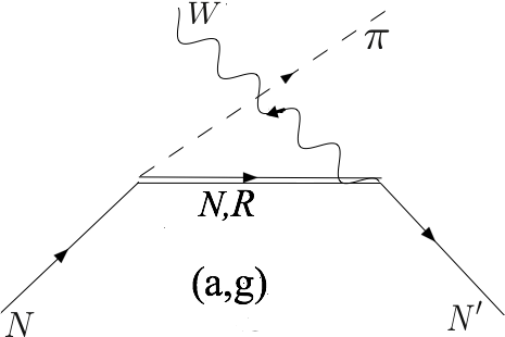
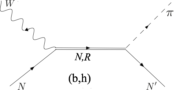
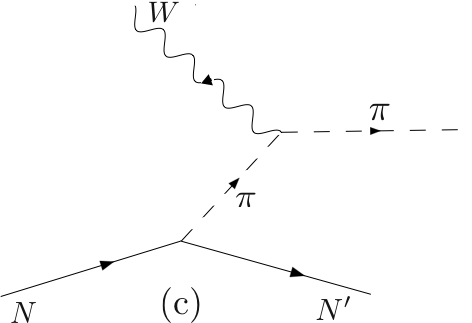
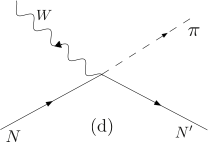
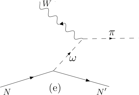
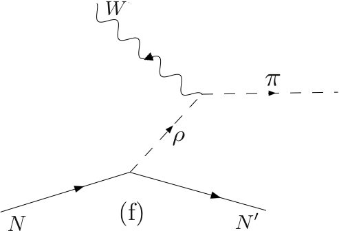
Figure 1: Terms in the scattering amplitude for the process $\nu(\bar{\text{$\nu$}})N\rightarrow\mu N^{\prime}\pi$. Terms (a) and (g) or (b) and (h) respectively, have the same tophological form with a nucleon (N) or any resonance (R) as intermediate states. Fig (a)-(g) represent the background (B) contribution. Fig (h) is a the direct or pole resonant contribution (R).

We can split $\mathcal{O^{\lambda}}$ as

$$\mathcal{O}^{\lambda} = \mathcal{O^{\lambda}}_{\text{B}}+\mathcal{O}_{\text{R}}^{\lambda},$$ (5)

where $\mathcal{O}_{B,R}$ generate the tree-level hadronic amplitudes contributing to the background (B), nucleon Born terms (Fig. 1(a)-(b)), the meson exchange amplitudes(contact term included) (Figs. 1(c)-(f)) and the resonance-crossed term (Fig. 1(g)); the direct or pole resonant contribution (R) is shown in Fig. 1(h) and it is neccesary the resonance adquires a width to avoid the singulatity in the propagator by a self energy dressing that can be treated within different approximations. The effect of the self energy could, in principle, change the full structure of the propagator. In the case of spin-$\frac{1}{2}$ resonances the unstable character introduced by this self energy accounts the replacement

$$m_{R} \rightarrow m_{R}-i\frac{\Gamma_{{}_{R}}(s)}{2},$$ (6)

into the unperturbed propagator without changing its structure. This width $\Gamma_{R}$ is obtained by considering the pion-nucleon loop contribution to the self energy Leitner09 (9) and reads

$$\Gamma_{R}(s)\times B_{r} = \frac{3}{4\pi}\left(\frac{f_{{}_{\pi NR}}}{m_{\pi}}\right)^{2}(m_{R}+\pi m_{N})^{2}\left(\frac{(\sqrt{s}-\pi m_{{}_{N}})^{2}-m_{{}_{\pi}}^{2}}{4s^{3/2}}\right)\lambda^{\frac{1}{2}}(s,m_{{}_{N}}^{2},m_{{}_{\pi}}^{2}),$$ (7)

$$\lambda(x,y,z) = x^{2}+y^{2}+z^{2}-2xy-2xz-2yz.$$

being $\pi=\pm$ the parity, $B_{r}$ the corresponding $\pi N$ branching ratio decay, and $f_{{}_{\pi NR}}$ the strong coupling.

For the spin-$\frac{3}{2}$ resonances the inclusion of the pion-nucleon loop in the self energy alters the full structure of the propagator due to the presence of spureous $\frac{1}{2}$ components. Nevertheless, if we neglect terms of order $\left(f_{{}_{\pi NR}}/{m_{\pi}}\right)^{4}$ and $((m_{R}-\sqrt{s})\left(f_{{}_{\pi NR}}/m_{\pi}\right)^{2})$ (see Ref.Barbero15 (27)), expected to be very small in the resonance region $(\sqrt{s}\approx m_{R})$, we keep the unperturbed form with the same replacement (6) and now

$$\Gamma_{{}_{R}}(s)\times B_{r} = \frac{\mathcal{I}_{R}\left(\frac{f_{{}_{\pi NR}}}{m_{\pi}}\right)^{2}}{4\pi}\left(\frac{(\sqrt{s}+\pi\times m_{{}_{N}})^{2}-m_{{}_{\pi}}^{2}}{48s^{5/2}}\right))\lambda^{\frac{3}{2}}(s,m_{{}_{N}}^{2},m_{{}_{\pi}}^{2}),$$ (8)

where $\mathcal{I}_{R}=\left\{\begin{array}[]{c}1\\ 3\end{array}\right.$ for $I=\left\{\begin{array}[]{c}\frac{1}{2}\\ \frac{3}{2}\end{array}\right.$ respectively.

If one analyzes the formal scattering T-matrix theory Mariano07 (28) for the final $\pi N$ pair in both elastic scattering or pion photoproduction, it is mandatory that the $\pi NR$ vertex should be also dressed as the propagator by the $\pi N$ rescattering through non-pole amplitudes. This makes also the vertex $s$-dependent, or in other words we get an effective coupling constant $\frac{f_{{}_{\pi NR}}(s)}{m_{\pi}}$, due to the decay Mariano07 (28) mediated by the intermediate $\pi N$-propagator (this will be analyzed deeply below). In previous works it has been have considered the approach resulting from the formal limit of massless $N$ and $\pi$ in the loop contribution to the $\Delta$ self energy and in the dressed $\pi N\Delta$ vertex. This was called the complex-mass scheme (CMS) Amiri92 (29). In this formal limit the vertex dressing gives a dependence $f_{{}_{\pi N\Delta}}(s)=\frac{\kappa f_{{}_{\pi N\Delta}}^{0}}{\sqrt{s}}$, being $f_{{}_{\pi N\Delta}}^{0}$ the bare $\pi N\Delta$ coupling constant and $\kappa$ a constant of dimension MeV to fit, in place of doing the complex calculation of the integral involved in the vertex correction. Within the CMS we derive from (8) the approximated expression ($B_{r}\approx 1$ for the $\Delta$)

$$\Gamma_{\Delta}(s) = \left(1-\frac{\sqrt{s}-m_{R}}{m_{R}}\right)\Gamma_{\Delta}^{CMS},\;\Gamma_{\Delta}^{CMS}=\frac{\kappa^{2}(\frac{f_{{}_{\pi NR}}^{0}}{m_{\pi}})^{2}}{192\pi}m_{\Delta}.$$ (9)

When $s\simeq m_{\Delta}^{2}$ we get a constant width $\Gamma_{\Delta}(s)\approx\Gamma_{\Delta}^{CMS}$, where $\Gamma_{\Delta}^{CMS}$ is fitted in place of $\kappa$ together $\frac{f_{{}_{\pi N\Delta}}}{m_{\pi}}$ and $m_{\Delta}$ to reproduce $\pi^{+}p$ scattering Mariano01 (30). Another approach commonly usedLeitner09 (9), is to fix $\sqrt{s}\approx m_{\Delta}$ in (7) or (8) and to use the experimental values for $m_{\Delta}$ and $\Gamma_{\Delta}$ times $B_{r}$, and get $f_{{}_{\pi NR}}$. We will refer to this as constant mass-width approach (CMW). We will use both the CMS and CMW depending on the considered resonance.

The explicit expressions for $\mathcal{O}_{B}$, splitted in those coming from the nucleon and meson exchange contributions (BN) and from the resonances(BR), and $\mathcal{O}_{R}$ for $R\equiv\Delta(1232)$, $N^{*}(1440),N^{*}(1520),N^{*}(1535)$ are shown in the Appendix. These are obtained in Ref.Tamayo22 (11). We only shown here the isospin factors for each contribution to the amplitude (see Fig.(1)) since it will be useful for the results section. They are indicated with $\mathcal{T}(m_{t}\equiv p,n,n,m_{t^{\prime}}\equiv p,p,n)$(or charge conjugate for $\bar{\nu})$ and can be obtained using the isospin operators present in the interaction Lagrangians togheter the isospin wave funcions for the $W$ boson and the hadrons (see Refs. Mariano11 (25) and Barbero08 (26) )

$$\mathcal{T}_{a} =\mathcal{T}_{g}^{1440,1535,1520}=-2,0,-\sqrt{2}$$

$$\mathcal{T}_{b} =\mathcal{T}_{h}^{1440,1535,1520}=0,-2,\sqrt{2}$$

$$\mathcal{T}_{c} =1,-1,\sqrt{2}$$

$$\mathcal{T}_{d} =-1,1,-\sqrt{2}$$

$$\mathcal{T}_{e} =-1,-1,0$$

$$\mathcal{T}_{f} =1,1,-\sqrt{2}$$

$$\mathcal{T}_{g}^{\Delta} =-1/3,-1,\sqrt{2}/3$$

$$\mathcal{T}_{h}^{\Delta} =-1,-1/3,-\sqrt{2}/3.$$ (10)

III Extension to higer $W_{\pi N}$ and and Results

In this work we analyse the total and differential cross sections for the charged current (CC) modes of the six processes

$$\nu p \rightarrow \mu^{-}p\pi^{+},\hskip 11.38092pt\nu n\rightarrow\mu^{-}p\pi^{0},\hskip 11.38092pt\nu n\rightarrow\mu^{-}n\pi^{+},$$

$$\bar{\nu}n \rightarrow \mu^{+}n\pi^{-},\hskip 11.38092pt\bar{\nu}p\rightarrow\mu^{+}n\pi^{0},\hskip 11.38092pt\bar{\nu}p\rightarrow\mu^{+}p\pi^{-},$$ (11)

with neutrino energies exciting the $W_{\pi N}=\sqrt{(p^{\prime}+k)^{2}}\leq 2$ GeV region. We will obtain these cross sections through the Eqs.(1-3) with the amplitude (4), taking $(1+\gamma_{5})$ when $\text{$\nu$}\rightarrow\bar{\nu}$, and the vertex production contributions in Eqs.(20-22) of the Appendix. We have included explicitly the resonances of the first and second region ($\Delta(1232),$$N^{*}(1440),N^{*}(1520),N^{*}(1535)$), while the effect of more energetic ones will be included indirectly. A calculation with the cuttoff $W_{\pi N}\lesssim 1.6$ GeV using the above mentioned CMS approach for the $\Delta(1232)$ and CMW for the other resonances, described properly $\sigma,\frac{d\sigma}{dQ^{2}},\frac{d\sigma}{dW_{\pi N}}$ Tamayo22 (11) for the ANL data. We have treated in consistent fashion the spin-$\frac{3}{2}$ resonances from the point of view of contact invariance and the true considered degree of freedom of the spin-$\frac{3}{2}$ field, both points mentioned in the introduction, choosing the values $A=-\frac{1}{3},Z=\frac{1}{2}.$ Now, we wish to extend our model to higher energies in order to describe the data of the recent reanalyzed ANL and BNL data without cutsRodriguez16 (18). On going to higher energies we can ask ourselves two important questions. First, is it possible to pursue the tree level model used for the background or the CMS and CMW approches to treat the resonances for any energy $W_{\pi N}$ with pointlike hadrons? Second, it is enough simply to add more and more resonances to describe the $W_{\pi N}>1.6$ GeV region? We will intend to analyze these questions within the frame of $\pi N$ rescattering, not considered in detail until now, in the following subsections.

III.1 Rescattering and hadrons FF

We support our discusion on the pion photoproduction reaction analyzed in Ref.Mariano07 (28), and we have the analogy $\mathcal{O}^{\lambda}\equiv\hat{B}^{\lambda}$ and $\mathcal{O}_{B,R}^{\lambda}\equiv\hat{B}_{NP}^{\lambda},\hat{B}_{P}^{\lambda}$ with the photoproduction vertexes in that reference. The approximation implemented previoulsy until the second resonance regionTamayo22 (11) can be resummed as

$$\mathcal{O}^{\lambda} \approx \mathcal{O}_{B}^{\lambda}+\mathcal{O}_{R}^{\lambda}\equiv\mathcal{O}_{B}^{\lambda}+\sum_{R}V_{R\pi N}G_{R}W_{WNR}^{\lambda},$$ (12)

where $V_{R\pi N}$ and $W_{WNR}^{\lambda}$ represent schematically the $R\rightarrow N\pi$ and $WN\rightarrow R$ vertexes respectively, while $G_{R}$ a resonance propagator. Nevertheless, the $\mathcal{O}_{B}^{{}^{\lambda}}$ contributions in special the $\mathcal{O}_{BR}^{\lambda}$ coming from the $\frac{3}{2}$ resonances (Fig.1(g)) can not be dressed by the self energy, being not affected by a $\pi N$ rescattering in (12) as done in $\mathcal{O}_{R}^{\lambda}$ with $\Gamma_{R}$. As consequence, grows rapidly for $W_{\pi N}\gtrsim 1.5$ GeV as will be shown below. As described in Ref.Mariano07 (28) for the case of photoproduction, but valid also here, there are other effects not considerated. The complete excitation amplitude in the final $\pi N$ CM is

$$\mathcal{O}^{\lambda}(k,q) = \left[-i(2\pi)^{4}\delta^{4}(k-k^{\prime})+T_{NP}(k^{\prime})G_{\pi N}(k^{\prime})\right]\left(\mathcal{O}_{B}^{\lambda}(k^{\prime},q)+\sum_{R}V_{R\pi N}(k^{\prime},k)G_{R}(k)\widetilde{W}_{WNR}^{\lambda}(k,q)\right)$$ (13)

$$\widetilde{W}_{WNR}^{\lambda}(k,q) = W_{WNR}^{\lambda}(k,q)+\left(V_{R\pi N}(k,k^{\prime\prime})+V_{R\pi N}(k,k^{\prime})G_{\pi N}(k^{\prime})T_{NP}(k^{\prime},k^{\prime\prime})\right)G_{\pi N}(k^{\prime\prime})\mathcal{O}_{B}^{\lambda}(k^{\prime\prime},q)$$ (14)

where $k^{\prime},k^{\prime\prime}$ are intermediate pion momenta and a repeated $k,k^{\prime},k^{\prime\prime}$ are indicate $i\frac{\int dk,k^{\prime},k^{\prime\prime 4}}{\left(2\pi\right)^{4}}$ ,

$$G_{\pi N}(k^{\prime}) = S_{N}(p+q-k^{\prime})\Delta_{\pi}(k^{\prime}),$$

is the pion-nucleon intermediate propagator, and $T_{NP}$ the non-pole scattering T-matrix that iterates to all orders the potential $V_{NP}\equiv V_{N\pi,N^{\prime}\pi^{\prime}}$ built with nucleon Born terms, meson exchange t-contributions and u-resonant contributions. In summary, in the full amplitude the rescattering of the final $\pi N$ pair through $T_{NP}$ is considered as well the decay into a resonance of $\mathcal{O}_{B}^{\lambda}$. We will not introduce in this work unitarizartion corrections, done through imaginary contributions in (13), since as we are analyzing the total and differential cross sections, where corrections to each multipole compensate out in the multipole expansion of the cross sectionMariano07 (28). As we wish to deal with effective real coupling constants ($T_{NP}$ dresses but is a complex operator), it is convenient to express the $\pi N$ T-matrix operator in terms of the real $K$-matrix Mariano07 (28), and after a three dimensional reduction we getMariano07 (28)

$$\mathcal{O}^{\lambda}(\boldsymbol{k},\boldsymbol{q},W_{\pi N}) \approx \left[(2\pi)^{3}\delta^{3}(\boldsymbol{k}-\boldsymbol{k^{\prime}})+\mathcal{P}\left(K_{NP}(\boldsymbol{k},\boldsymbol{k}^{\prime})G_{TH}(\boldsymbol{k}^{\prime},\sqrt{s})\right.\right]$$ (15)

$$\times \left[\left.\mathcal{O}_{B}^{\lambda}(\boldsymbol{k}^{\prime},\boldsymbol{q},W_{\pi N})\right)+\sum_{R}\left.V_{R\pi N}(\boldsymbol{k}^{\prime},\boldsymbol{p})\right)G_{R}(\boldsymbol{p},W_{\pi N})\widetilde{W}_{WNR}^{\lambda}(\boldsymbol{p},\boldsymbol{q},W_{\pi N})\right],$$

$$\widetilde{W}_{WNR}^{\lambda}(\boldsymbol{p},\boldsymbol{q},W_{\pi N}) = W_{WNR}^{\lambda}(\boldsymbol{p},\boldsymbol{q})+\mathcal{P}\left[V_{R\pi N}(\boldsymbol{p},\boldsymbol{k^{\prime}})G_{TH}(\boldsymbol{k^{\prime}},W_{\pi N})\mathcal{O}_{B}^{\lambda}(\boldsymbol{k^{\prime}},\boldsymbol{q})\right],$$ (16)

where $G_{\pi N}(k^{\prime})$ is replaced by the Thompson propagator $G_{TH}(\boldsymbol{k^{\prime}},W_{\pi N})=\frac{m_{N}}{2E_{\pi}(\boldsymbol{k^{\prime}})E_{N}(\boldsymbol{k^{\prime}})}\sum_{ms^{\prime}}\frac{u(-\boldsymbol{k^{\prime}},m_{s}^{\prime})\bar{u}(\boldsymbol{k^{\prime}},m_{s}^{\prime})}{W_{\pi N}-E_{\pi}(\boldsymbol{k^{\prime}})-E_{N}(\boldsymbol{k^{\prime}})}$ and where with $\mathcal{P}$ is the principal value on the integral in reapeated momenta.

In order to reproduce the experimental data FF have to be introduced which affect both $\mathcal{O}_{B,R}^{{}^{\lambda}}$ to regularyze the integrals in (15) and (16) . They are meant to model the deviations from the pointlike couplings due to the quark structure of nucleons and resonances, analogs of the electromagnetic ones reflecting the extension of the hadrons, and should be calculated from the underlying theory or quark modelsMelde09 (31). Because it is not clear a priori which form these additional factors should have, they introduce a source of systematical error in all modelsMosel98 (32). Guided by an our previous proper description on NC1$\pi$ data obtained by the CERN Gargamelle experiment without applying cuts in the neutrino energiesMariano11 (25), we multiply $\mathcal{O}_{B}^{\lambda}+\mathcal{O}_{R}^{\lambda}$ by a global regularyzing FF of the $R\pi N$ and $N\pi N^{\prime}$ vertexes (${\rm k}=|\boldsymbol{k}|$)

$$F({\rm k},W_{\pi N}) = \frac{\left(\Lambda\right)^{4}}{\left(\Lambda\right)^{4}+{\rm k(W_{\pi N})^{2}}\left(W_{\pi N}-W_{\pi N}^{th}\right)^{2}\theta(W_{\pi N}-1.6\mbox{{GeV}})},$$ (17)

$$\mathrm{\>k}(W_{\pi N}) = \sqrt{\frac{(W_{\pi N}^{2}-m_{N}^{2}-m_{\pi}^{2})^{2}-4m_{N}^{2}m_{\pi}^{2}}{4W_{\pi N}^{2}}},$$ (18)

being the threshold invariant mass $W_{\pi N}^{th}=m_{\pi}+m_{N}$ and which is consistent with that introduced in Refs.Sato96 (33) and Pearce91 (34)(footnote (35)), but lighting it above the second resonance region since it was shown that the description with the $W_{\pi N}\lesssim 1.6$ GeV was correct within our model Tamayo22 (11). This FF can be seen as

$$F({\rm k},W_{\pi N}) = \frac{\left(\Lambda_{eff}\right)^{2}}{\left(\Lambda_{eff}\right)^{2}+{\rm k(W_{\pi N})^{2}}},\Lambda_{eff}=\Lambda\frac{\Lambda}{W_{\pi N}-W_{\pi N}^{th}},$$ (19)

where we have a monopole FF with an effective cutoff diminishing with $W_{\pi N}-W_{\pi N}^{th}$, making that certain term ”disappears” or contributes less in the amplitude since when $W_{\pi N}$ grows another resonance, not considered in the amplitude, could be excited. Note that this FF affects also the on-shell contributions,i.e, the terms surviving in (15) when the $\mathcal{P}$ terms are dropped.

In resume, to get the full amplitudes in Eq.(15) we need to add FF taking into account the hadron extensions since as can be seen in $G_{TH}(\boldsymbol{k^{\prime}},W_{\pi N})$, we keep the $\pi$ and $N$ elemental character for any $W_{\pi N}$, and this makes the involved integral divergent. This entails to moderate the on shell amplitude $\mathcal{O}^{\lambda}$ with this FF, which is not considered in the approach (12).

III.2 Results

We adopt the same model as in a recent workTamayo22 (11), where we have calculated the pion production cross section including explicitly spin-$\frac{1}{2}$ and $\frac{3}{2}$ resonances $\Delta(1232),N^{*}(1440),N^{*}(1520)$ and $N^{*}(1535)$ in the calculus of the amplitudes(20),(21) and (22) in the Appendix to cover the so called second resonance region. The formal aspects mentioned in the introduction an related with the spin-$\frac{3}{2}$ Lagrangians (free and interaction) regards the contact-transformation parameter and the additional $Z$ parameter present in the $\mathcal{L}_{\pi NR}$ interaction lagrangian, have been discussed in that reference. The non resonant contributions in (20) are also described in Tamayo22 (11) together all the adopted FF. We treat the spin-$\frac{1}{2}$ resonances within the parity conserving parametrization for the FF, since this is compatible to that used in the similar topologycal nucleon contribution in Fig.1 (a) and (b). For the spin-$\frac{3}{2}$ resonances we use the Sachs parametrization to be consistent with our previous works including only the $\Delta$ resonance, where we get better results than using the parity conserving oneBarbero14 (36). We followed the conexion between both parametrizations achieved in that reference to get the FF for the $N^{*}(1520)$ resonance, and have taken the $Q^{2}$-depedent FF from Ref.Lakakulich06 (37) for all the second region resonances. The main channel $\nu p\longrightarrow\mu^{-}\pi^{+}p^{\prime}$ with the cut $W_{\pi N^{\prime}}<1.4$ GeV in the final invariant mass, is used to fix the main axial $\Delta$-coupling constant $D_{1}(0)$ Refs.Mariano07 (28, 26). With this cut it was shown Tamayo22 (11), at less for this channel, that the contributions of more energetic resonances than the $\Delta(1232)$ are small and that are important only for more energetic cuts. As the reanalyzed data of ANL achieved in Ref.Rodriguez16 (18) does not affect appreciably the channel used to fit $D_{1}(0)$ for $W_{\pi N^{\prime}}<1.4$ GeV, then we will not make a new fitting to $\left\langle\frac{d\sigma}{dQ^{2}}\right\rangle$. In our previous work Tamayo22 (11) we achieved the comparison with the data of ANL experiment in the region of $W_{\pi N}<1.4,1.6$ GeV, where we have worked within the CMS+CMW approach. From the results including and not including the second resonance region, we concluded that to describe the data in all channels this resonance region should be included. We concluded that these resonances influence through their tails, since they have their centroids over these cuts. At the amplitude level, these tails interfere with the another resonances and background contributions. This behavior is confirmed when we compared with the data with the $W_{\pi N}<1.6$ GeV and the good agreement with the data for the antineutrino case.

Nevertheless, the ANL data of Ref.Rad82 (6) contains also results without energy cuts and also all results in Ref.Kitagi86 (7) are reported without events exclusion. In addition, the reanalysis of these two set of data has been done recently in Refs.wilki14 (17, 18) where the main results of the cross section are obtained with a tunable invariant mass value, which is W $\leq$ 1.7 GeV by and compared with data without cuts. For describing them we need to extend our model to higher energies. The main question seems to be, do we add more energetic resonances keeping the approach in Eq.(12)? or do we put attention on the FF discussion in the previous subsection? In the Fig.(2) we show the total cross section (1) calculated with the amplitude (4) obtained from the approach (12) and Eqs.(20-22) in the Appendix. Now we enable that $W_{\pi N}\lesssim 2$ GeV, as can be seen the cross section grows with a departure from the data. With full lines we show the results of the CMS + CMW approach for the resonances with a constant width, while with dashed lines we show results used the same masses $m_{R}$ and coupling constants $f_{\pi NR}$ but with energy dependent widths given by Eqs.(7) and (8). As can be seen a better width’s approach, what means a most exact treatment in the resonance self energy, improves appreciably the description for the first channel. In it, the direct contribution (Fig.1(h)) for the $\Delta$ with$\mathcal{T}_{h}^{\Delta 2}=1$ in Eq.(10), is the main contribution being the cross one with $\mathcal{T}_{g}^{\Delta 2}=1/9$ very small. For the other two channels, this contribution is much lower since $\mathcal{T}_{h}^{\Delta 2}=1/9,2/9$ and the background contribution with $\mathcal{T}_{g}^{\Delta 2}=1,2/9$ is the most or at least equal important.

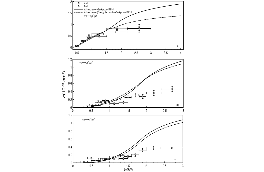
Figure 2: Total $\nu N$ cross section as function of the neutrino energy for different channels and $F({\rm k},W_{\pi N})=1$. Results with $\Delta+$second region resonances plus the corresponding background in each case are shown for a cut $W_{\pi N}\lesssim 2$ GeV with dotted and full lines. Results within CMS+CMW and with energy dependent width with are shown with dashed lines. Data are taken form Ref.Rad82 (6)

These cross terms contribute to the background and cannot dressed by the $\Delta$ self energy. The same kind of analysis can be done for the other $\frac{1}{2}$-resonances, that have the same isospin factors that the direct and cross nucleon terms (Figs.1(b) and (a)), but with a much lower contribution of these regards the $\Delta$. This analysis is an indication that to include rescattering effects could be more important that to add more and more energetic resonances, since background contributions will grow anyway. In resume, all background contributions coming from non-resonant origin plus cross-resonant terms (Figs.1(a)-1(g)) cannot be dressed by a self energy and its behavior could be corrected taking into account the rescattering through $T_{NP}$ as discussed in the previous subsection.

As was mentioned, in Eqs. (15) and (16) $\mathcal{O}^{\lambda}$ should be effected by a FF. As to solve numerically the $\mathcal{P}$-integrals is not trivial, we will assume the minimum approach of considering :

a) The use of effective couplings in $W_{WNR}^{\lambda}$, that is $\widetilde{W}_{WNR}^{\lambda}\rightarrow W_{WNR}^{\lambda}(\mbox{{effective\>weak\>couplings}})$ to simulate the effect of the second term of Eq.(16), that was shown satisfactory for the case of photoproductionMariano07 (28). These effective values are the empirical one adopted in our previous work Tamayo22 (11). Same will be valid for $\mathcal{O}_{B}^{\lambda}$ where weak empirical or experimental coupling constants are used.

b)To avoid model dependencies coming from the introduction of arbitrary FF at each interaction vertex, we will introduce a global form factor (17) in the decay amplitude. The using of FF at each vertex requires the introduction of vertex corrections to keep for example electromagnetic gauge invariance. As we are including resonances with effects ultil around $W_{\pi N}\sim 1.6$ GeV, taking into account the width of the most energetic considered one($S_{11}(1535)$ MeV), we will only light on this FF above this energy.

In this way, we also correct the amplitude for excitation of more energetic resonances not considered, through the effective monopole form in Eq.(19)(see the followed discussion), in our model since now we wish describe data without $W_{\pi N}$ cuts. Guided by a previous proper description on NC1$\pi$ data obtained by the CERN Gargamelle experiment without applying cuts in the neutrino energiesMariano11 (25), we multiply $\mathcal{O}_{B}^{\lambda}+\mathcal{O}_{R}^{\lambda}$ by a global regularyzing FF of the $\Delta\pi N$ and $N\pi N^{\prime}$ vertexes described above in Eq.(17). We adopt the value $\Lambda=600$ MeV in consistence with Ref.Mariano11 (25). Also we throw out the $\mathcal{P}$ contribution in the first bracket of Eq.(15) modifying only the onshell potential, as a first minimum modification to the model and that was appropiated when we discussed NC1$\pi$Mariano11 (25). In resume, this FF should take into account the hadron structure and the posibility of exciting more energetic resonances, when $W_{\pi N}$ grows, in an effective fashion.

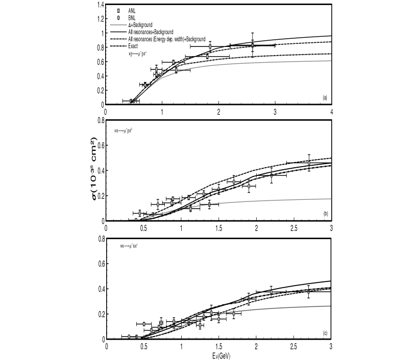
Figure 3: Total $\nu N$ cross section as function of the neutrino energy for different channels. Results with only the $\Delta$ and all resonances = $\Delta+$second region’s resonances, plus the corresponding background are shown for $W_{\pi N}\lesssim 2$ GeV. Data are taken from the reanalyzed ANL and BNL ones in Ref.Rodriguez16 (18). $\Delta+$background in CMS, dotted lines. All resonances + background in CMS+CMW, full lines. Same but with energy dependent width from Eqs.(7,8), dashed lines. Finally, same but using the exact expresion for the $\Delta$ propagator (see. Ref.Barbero14 (36)), dashed-dotted lines

Now, we discuss with more detail the calculations with $W_{\pi N}\lesssim 2$ GeV and compare with data without cuts. As we have seen in the previous Fig.(2) the model used to treat the self energy in the propagators leads to different results. Firstly, we will use the CMS+CMW approaches that assume a constant width, secondly kepping the same propagators but with the energy dependet width in Eqs.(7) and (8), and finally we assume the exact $\Delta$(that is the main contributing one) propagator. In this last case, the self energy change the structure of the $\Delta$ propagatorBarbero14 (36) but we assume the simplification of using the same effective mass and width of the the CMS approach. Results are shown in the Figure(3). As can be seen, the tendency of increasing the cross section by the second resonance region contribution is persistent as previously Tamayo22 (11), and the results that better reproduce globally the three channels the data is still the CMS+CMW approach with constant width. When we enable an energy dependent width, we see a change that depends on the channel diminishing the results in the main one (first pannel of Fig.(3 )) and growing and diminishing in the other two (second an third pannels of Fig.(3 )). When the exact propagator for the $\Delta$ is used, the results for the first channel is more diminished and an opposite effect is generated for the other two one. Nevertheless, an observation should be done in order. The parameters used for the $\Delta$ resonance ($f_{\pi N\Delta},m_{\Delta},\Gamma_{\Delta},$ $G_{E},G_{M},D_{1}\mbox{ or }C_{A}^{5}$) have been fitted using the CMS approach with a constant width, and thus if one wish to use another approach a new fitting should be done.This could explain why the best fit is done with the simpler CMS approach, while for the energy dependent width should be not crucial a change of parameters since we are keeping the same structure of the CMS propagator. In addition, as we are using a global FF that affects the full amplitude, and if the other resonances are treated within the CMW approach, to use an exact propagator for the $\Delta$ would be no so consistent. Finally, it is evident that the FF taken from NC pion productions also works very well here.

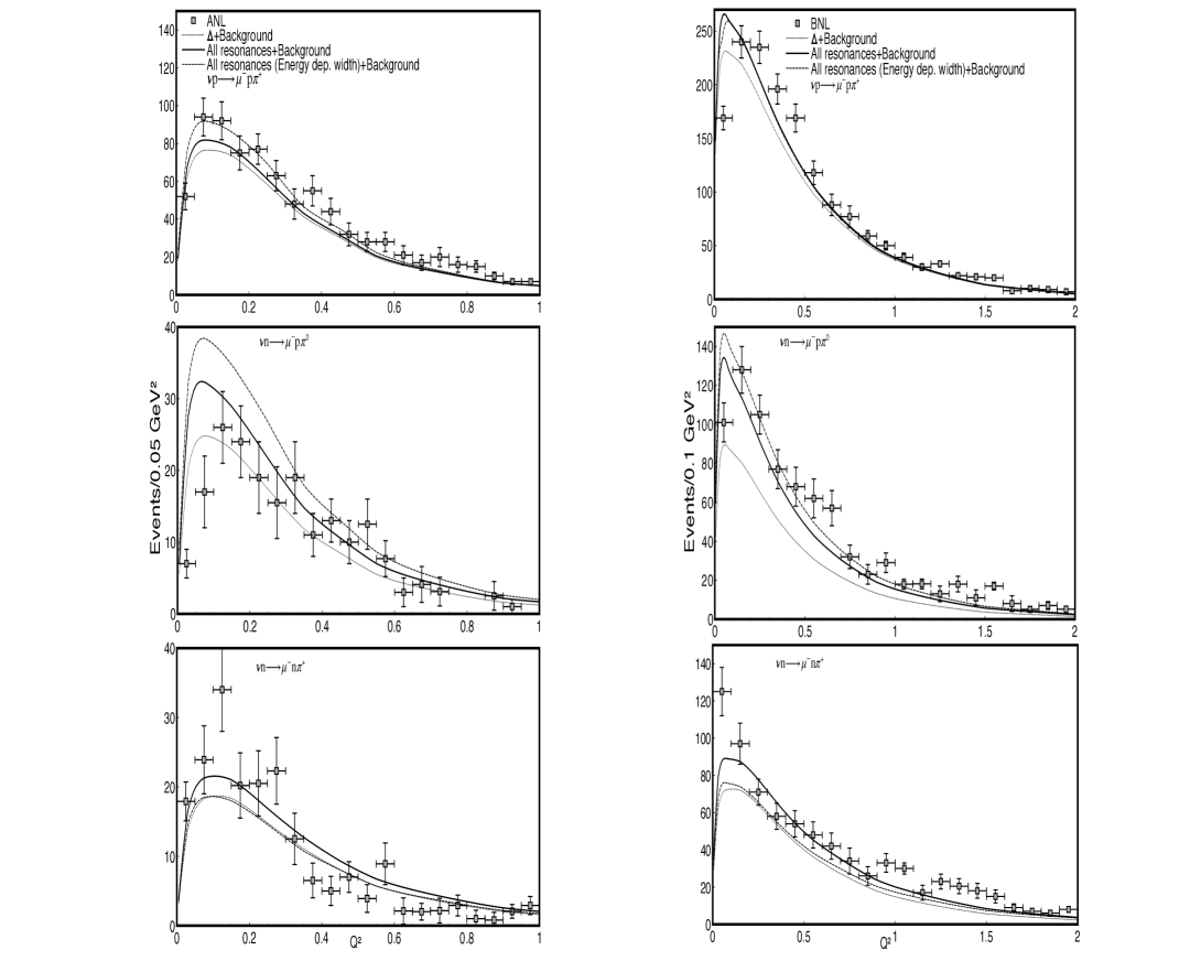
Figure 4: Differential cross section with $W_{\pi N}\lesssim 2GeV$. Lines convention are the same that in previous Fig.(3). Data are taken from Ref.Rodriguez16 (18).

This is supported by the following analysis. We have shown previously in the Ref. Mariano11 (25) , from where the parameter $\Lambda$ in Eq.(19) was taken, the effect of the uncertainties in the parameters $D1(0)$ and $M_{A}$ in the axial FF for the $\Delta$ resonance within the CMS model through a hatched area in the Figs.(7) and (8). There, it was shown that the uncertainties effects on the results is well below the data errors and the differences when we change from energy dependent to constant widths approaches. These two parameters where involved in the fitting we done on the flux averaged $d\sigma/dQ^{2}$ cross section in the previous Ref. Barbero08 (26) and then used in the following contributions, while the axial coupling for the another resonances were fixed from the PDG values for masses and widths. As we are not doing any new fitting here but using the parameters of previous works, we felt not necessary to analyzed the CMS+CMW parameters uncertainties effects again, because they are under control.

As the fitting of the axial $\Delta$ parameters it is achieved using the flux averaged diferential cross section $<d\sigma/dQ^{2}>$, we show the results for it within our model and compare with the more recent ANL and BNL reanalyzed data Rodriguez16 (18). In that reference results are shown for the events-$Q^{2}$ distribution in units of Events/GeV² and as our results are given in $10^{-38}$cm${}^{2}/$GeV² we use the same conversion factor found in the total cross section calculation to compare with the data. They are reported without cuts and are compared with our results in Fig.(4). We show calculations within the same approaches than the total cross section, but avoid to use the exact $\Delta$ propagator for the reasons exposed above. As can be seen, results within the constant width are acceptable in the three channels. We are not doing any new fit (the fixing of $C_{A}^{5}$was done previuolsy Mariano01 (30) using the ANL data with cuts $W_{\pi N}<1.4$ GeVRad82 (6)), and the description is better that those done with GENIE in Ref. Rodriguez16 (18). As can be seen the using of energy dependent width enlarges the first and second channels theoretical results and diminishes those for the third one, this leads to a worse coincidence with data in an amount depending on the experiment ANL or BNL.

III.3 ANTINEUTRINOS

Now, in order to follow probing our model we wish to calculate the antineutrinos total cross section as done in our previous workTamayo22 (11). We have to differences regards the neutrinos case. Firstly the interactions of neutrinos with hadrons is not the same that for antinetrinos. We have a sign of difference in the lepton current contraction that makes a different coupling with the hadron one. Then, the interaction with neutrinos is different from antineutrinos due the use of spinors for antiparticles in the lepton current in Eq.(4) and has nothing to do with the very know CP violation. Secondly, in the experiment an admixture of heavy freon CF3Br was exposed to the CERN PS antineutrino beam (peaked at $E_{\bar{\nu}}\sim$ 1.5 GeV). In this case, the experiment informs that we have 0.44% on neutrons and 0.55% of protons, and since our calculations were for free nucleons we weight out results with these precentages depending on the channel. Our results including all resonances and for $W_{\pi N}\lesssim 2$ GeV are compared with the data reported inBolog79 (38) are shown in Fig.(5) , and as can be seen we get a consistent description with that for the neutrino case.

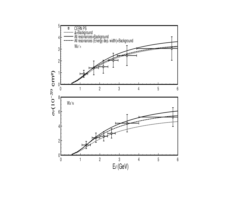
Figure 5: Antineutrino’s total cross sections with a $W_{\pi N}\lesssim 2$ GeV for the $\bar{\nu}n\rightarrow\mu^{+}n\pi^{-}$ and that leadding to a final $N\pi^{-}$final state. Lines conventions are the same that in Fig.(3).

We show results within the CMS with only the $\Delta$ and the $\Delta$ with the other resonances in the CMW, showing an appreciable difference between the different approaches. Adding the energy dependent width we get an improvement, but anyway we have consitence with the neutrino’s results.

IV. CONCLUSIONS

We have extended our dynamical model including resonances into the first and second region, previously used to describe succesfully neutrino and antineutrino scattering cross sections ANL data with the cuts $W_{\pi N}\lesssim 1.4,1.6$ GeV, to describe ANL and BNL data without cuts. The model treats consitently the vertexes and propagators for the spin-$\frac{3}{2}$ resonances from the point of view of contact transformations of the spin-$\frac{3}{2}$ $\Psi_{\mu}$ field and the role of the $\Psi_{0}$ component. In addition, we incorporate the different pole resonant contributions and background resonant and non-resonant ones, in a coherently sum to the amplitude. We have added a global effective monopole FF to take into account the hadrons size and possible more energetic resonances excitations not included explicitly in the model for $W_{\pi N}\lesssim 2.$GeV. The data to compare, are that reanalyzed to eliminate flux normalization incertainties in the ANL and BNL experiments wilki14 (17, 18). In GENIE simulation to describe the mentioned data Rodriguez16 (18), single pion production is separated into resonant and non-resonant terms, with interference between them neglected and interferences between resonances neglected too in the calculation. The resonant component is a modified version of the RS model Rein81 (20), where the production and subsequent decay of 18 nucleon resonances with invariant masses$W\leq 2$ GeV are considered. In GENIE, only 16 resonances are included, based on the recommendation of the Particle Data Group PDG06 (39). In this work they make the assumption that interactions on deuterium can be treated as interactions on quasi-free nucleons which are only loosely bound together, and so neglect FSI effects. In GENIE, there are a number of systematic parameters which can be varied to change the single pion production model. Resonant axial mass ($M_{A}^{RES}$) Resonant normalization (RES norm) Non-resonant normalization (DIS norm), and normalization of the axial form factor ($F_{A}(0)$). The total GENIE prediction is the incoherent sum of the RES and DIS contributions, where interference terms have been neglected. GENIE cannot describe all of the pion production channels well for the reanalyzed datasets. For example, the data of the $\nu_{\mu}n\rightarrow\mu^{-}p\pi^{0},\nu_{\mu}n\rightarrow\mu^{-}n\pi^{+}$ channels are very similar, but there are large differences between the nominal GENIE predictions for these channels. The non-resonant component of the GENIE prediction, which contributes strongly to these channels, appears to be too large. Nevertheless, within our model these two channels are described properly. Finally, it can be seen from Fig.(3) of Ref.Rodriguez16 (18), where neutrino energy distribution is shown, that the nominal GENIE prediction fails to describe the low-$Q^{2}$ data well for some channels.We also note that the GENIE uncertainties are larger than the data suggests, and they may be reduced by tuning the GENIE model to the ANL and BNL data. At difference, within our model the low $Q^{2}$ distribution seem to be right. In addition, we describe also and properly antineutrino cross section without cuts in the data. In resume, its seem that keeping control on the cross sections until the second resonance region ($W_{\pi N}\lesssim 1.6$ GeV), enables a good description without cuts introducing the effect of finite size of hadrons and more energetic resonances in an effective way.

IV Appendix

The background contributions to the amplitude read

$$O_{\text{B}}^{\lambda}(p,p^{\prime},q) = O_{\text{BN}}^{\lambda}(p,p^{\prime},q)+O_{\text{BR}}^{\lambda}(p,p^{\prime},q)$$

$$O_{\text{BN}}^{\lambda}(p,p^{\prime},q) = -i\frac{1}{2}\Bigg{[}F_{1}^{V}(Q^{2})\gamma^{\lambda}-i\frac{F_{2}^{V}(Q^{2})}{2m_{{}_{N}}}\sigma^{\lambda\nu}q_{\nu}-F^{A}(Q^{2})\gamma^{\lambda}\gamma_{{}_{5}}\Bigg{]}i\frac{\not\!p^{\prime}+\not\!q+m_{{}_{N}}}{(p^{\prime}+q)^{2}-m_{{}_{N}}}$$ (20)

$$\times \frac{g_{{}_{\pi NN}}}{2m_{{}_{N}}}\gamma_{{}_{5}}(\not\!p-\not\!p^{\prime}-\not\!q)\sqrt{2}\mathcal{T}_{a}(m_{t},m_{t^{\prime}})$$

$$+ \frac{g_{{}_{\pi NN}}}{2m_{{}_{N}}}\gamma_{{}_{5}}(\not\!p-\not\!p^{\prime}-\not\!q)i\frac{\not\!p-\not\!q+m_{{}_{N}}}{(p-q)^{2}-m_{{}_{N}}^{2}}\left(-i\frac{1}{2}\right)\Bigg{[}F_{1}^{V}(Q^{2})\gamma^{\lambda}-i\frac{F_{2}^{V}(Q^{2})}{2m_{{}_{N}}}\sigma^{\lambda\nu}q_{\nu}-F^{A}(Q^{2})\gamma^{\lambda}\gamma_{{}_{5}}\Bigg{]}$$

$$\times \sqrt{2}\mathcal{T}_{b}(m_{t},m_{t^{\prime}})$$

$$- \frac{i}{(p-p^{\prime})^{2}-m_{\pi}^{2}}iF_{1}^{V}(Q^{2})(2p-2p^{\prime}-q)^{\lambda}\times\frac{g_{{}_{\pi NN}}}{2m_{{}_{N}}}\gamma_{{}_{5}}(\not\!p-\not\!p^{\prime})\sqrt{2}\mathcal{T}_{c}(m_{t},m_{t^{\prime}})$$

$$+ \frac{g_{{}_{\pi NN}}}{2m_{{}_{N}}}F_{1}^{V}(Q^{2})\gamma_{{}_{5}}\gamma^{\lambda}\sqrt{2}\mathcal{T}_{d}(m_{t},m_{t^{\prime}})$$

$$+ i\frac{g_{{}_{\omega\pi V}}}{m_{\pi}}F_{1}^{V}(Q^{2})\epsilon^{\lambda\alpha\beta\delta}q_{{}_{\alpha}}(p-p^{\prime})_{{}_{\beta}}i\frac{-g_{{}_{\delta\epsilon}}}{(p-p^{\prime})^{2}-m_{\omega}^{2}}(-i)\frac{g_{{}_{\omega NN}}}{2}\Bigg{[}\gamma^{\epsilon}-i\frac{\kappa_{\omega}}{2m_{{}_{N}}}\sigma^{\epsilon\kappa}(p-p^{\prime})_{\kappa}\Bigg{]}$$

$$\times \sqrt{2}\mathcal{T}_{e}(m_{t},m_{t^{\prime}})$$

$$+ f_{\rho\pi A}F^{A}(Q^{2})i\frac{-g^{\lambda\mu}}{(p-p^{\prime})^{2}-m_{\rho}^{2}}(-i)\frac{g_{{}_{\rho NN}}}{2}\Bigg{[}\gamma_{\mu}-i\frac{\kappa_{\rho}}{2m_{{}_{N}}}\sigma_{\mu\kappa}(p-p^{\prime})^{\kappa}\Bigg{]}\sqrt{2}\mathcal{T}_{f}(m_{t},m_{t^{\prime}}),$$

$$O_{\text{BR}}^{\lambda}(p,p^{\prime},q) =- i\frac{1}{2}\Bigg{[}\frac{g_{1V}^{1440}}{(m_{{}_{1440}}+m_{{}_{N}})^{2}}(Q^{2}\gamma^{\lambda}+\not\!qq^{\lambda})-\frac{g_{2V}^{1440}}{(m_{{}_{1440}}+m_{{}_{N}})}i\sigma^{\lambda\nu}q_{\nu}-g_{1A}^{1440}\gamma^{\lambda}\gamma_{5}+\frac{g_{3A}^{1440}}{m_{{}_{N}}}q^{\lambda}\gamma_{5}\Bigg{]}$$ (21)

$$\times i\frac{\not\!p^{\prime}+\not\!q+m_{R}}{(p^{\prime}+q)^{2}-m_{1440}^{2}+i\Gamma_{1440}m_{1440}}(-)\frac{f_{{}_{1440\pi N}}}{m_{\pi}}\gamma_{5}(\not\!p-\not\!p^{\prime}-\not\!q)\sqrt{2}\mathcal{T}_{g}^{1440}(m_{t},m_{t^{\prime}})$$

$$- i\frac{1}{2}\gamma_{5}\Bigg{[}\frac{g_{1V}^{1535}}{(m_{{}_{1535}}+m_{{}_{N}})^{2}}(Q^{2}\gamma^{\lambda}+\not\!qq^{\lambda})-\frac{g_{2V}^{1535}}{(m_{{}_{1535}}+m_{{}_{N}})}i\sigma^{\lambda\nu}q_{\nu}-g_{1A}^{1535}\gamma^{\lambda}\gamma_{5}+\frac{g_{3A}^{1535}}{m_{{}_{N}}}q^{\lambda}\gamma_{5}\Bigg{]}$$

$$\times i\frac{\not\!p^{\prime}+\not\!q+m_{1535}}{(p^{\prime}+q)^{2}-m_{1535}^{2}+i\Gamma_{1535}m_{1535}}(-)\frac{f_{{}_{1535\pi N}}}{m_{\pi}}(\not\!p-\not\!p^{\prime}-\not\!q)\sqrt{2}\mathcal{T}_{g}^{1535}(m_{t},m_{t^{\prime}})$$

$$+ (-\overline{){W_{\lambda\alpha}^{WN\Delta}(p,p^{\prime},-q)}}iG_{\Delta}^{\alpha\beta}(p^{\prime}+q)(-)\frac{f_{{}_{\Delta\pi N}}}{m_{\pi}}(p-p^{\prime}-q)_{\beta}\sqrt{2}\mathcal{T}_{g}^{\Delta}(m_{t},m_{t^{\prime}})$$

$$+ (-\overline{){\frac{1}{2}W_{\lambda\alpha}^{WN1520}(p,p^{\prime},-q)}}iG_{1520}^{\alpha\beta}(p^{\prime}+q)(-)\frac{f_{{}_{1520\pi N}}}{m_{\pi}}\gamma_{5}(p-p^{\prime}-q)_{\beta}\sqrt{2}\mathcal{T}_{g}^{1520}(m_{t},m_{t^{\prime}}),$$

where $\frac{1}{2}$-resonances the are put before the $\frac{3}{2}$-ones. $G_{R}^{\alpha\beta}$ togheter $W^{WNR}=\left(V^{WNR}+A^{WNR}\right)$are the spin-$\frac{3}{2}$ resonance propagators and $WN\rightarrow R$ vertexes respectively, both defined in Ref.Tamayo22 (11) while $\overline{W}=\gamma_{0}W^{\dagger}\gamma_{0}$ . $V^{WNR}$ is the vector vertex as in pion-photo($Q^{2}=0)$Mariano07 (28) and electroproduction applying CVC within the Sachs parametrization, and $A^{WNR}$ the axial contribution compatible with $V_{\nu\mu}^{WN\Delta}$ Barbero08 (26)(it could be, in principle, obtained by using $-V_{\nu\mu}^{WN\Delta}\gamma_{{}_{5}}$).
The corresponding pole contributions coming from the resonances are

$$\mathcal{O}_{R}^{\lambda} = \frac{f_{{}_{1440\pi N}}}{m_{\pi}}\gamma_{5}(\not\!p-\not\!p^{\prime}-\not\!q)i\frac{\not\!p-\not\!q+m_{R}}{(p-q)^{2}-m_{1440}^{2}+i\Gamma_{1440}m_{1440}}$$ (22)

$$\times (-i)\frac{1}{2}\Bigg{[}\frac{g_{1V}^{1440}}{(m_{{}_{1440}}+m_{{}_{N}})^{2}}(Q^{2}\gamma^{\lambda}+\not\!qq^{\lambda})-\frac{g_{2V}^{1440}}{(m_{{}_{1440}}+m_{{}_{N}})}i\sigma^{\lambda\nu}q_{\nu}-g_{1A}^{1440}\gamma^{\lambda}\gamma_{5}+\frac{g_{3A}^{1440}}{m_{{}_{N}}}q^{\lambda}\gamma_{5}\Bigg{]}\sqrt{2}\mathcal{T}_{h}^{1440}(m_{t},m_{t^{\prime}})$$

$$+ (-)\frac{f_{{}_{1535\pi N}}}{m_{\pi}}(\not\!p-\not\!p^{\prime}-\not\!q)i\frac{\not\!p-\not\!q+m_{1535}}{(p-q)^{2}-m_{1535}^{2}+i\Gamma_{1535}m_{1535}}$$

$$\times (-i)\frac{1}{2}\Bigg{[}\frac{g_{1V}^{1535}}{(m_{{}_{1535}}+m_{{}_{N}})^{2}}(Q^{2}\gamma^{\lambda}+\not\!qq^{\lambda})-\frac{g_{2V}^{1535}}{(m_{{}_{1535}}+m_{{}_{N}})}i\sigma^{\lambda\nu}q_{\nu}-g_{1A}^{1535}\gamma^{\lambda}\gamma_{5}+\frac{g_{3A}^{1535}}{m_{{}_{N}}}q^{\lambda}\gamma_{5}\Bigg{]}\gamma_{5}\mathcal{T}_{h}^{1335}(m_{t},m_{t^{\prime}})$$

$$+ (-)\frac{f_{{}_{\Delta\pi N}}}{m_{\pi}}(p-p^{\prime}-q)_{\alpha}iG_{\Delta}^{\alpha\beta}(p-q)W_{\beta\lambda}^{WN\Delta}(p,p^{\prime},q)\sqrt{2}\mathcal{T}_{g}^{\Delta}(m_{t},m_{t^{\prime}})$$

$$+ (-)\frac{f_{{}_{1520\pi N}}}{m_{\pi}}\gamma_{5}(p-p^{\prime}-q)_{\alpha}iG_{\Delta}^{\alpha\beta}(p-q)W_{\beta\lambda}^{WN1520}(p,p^{\prime},q)\sqrt{2}\mathcal{T}_{g}^{1520}(m_{t},m_{t^{\prime}}),$$

where all the vector and axial weak FF present in Eqs.(20-22) are defined in Ref.Tamayo22 (11). Note that the $\frac{1}{2}$ factor in the weak vertex of the spin-$\frac{1}{2}$ resonances comes from the isovector part of the charge operator $\frac{\tau_{3}}{2}$ dragged from the CVC hypotesis.

V Acknowledgments

A. Mariano belong to CONICET and UNLP, D.F. Tamayo Agudelo and D.E. Jaramillo Arango to UdeA.

References

- (1) 1. B.Eberly et al.,Phys.Rev.D92(9),092008(2015).
- (2) T.Le et al.,Phys.Lett.B749,130(2015).
- (3) A. Aguilar-Arevalo et al., Phys. Rev. D 83, 052007 (2011).
- (4) J.T.Sobczyk,J.Z˙muda,Phys.Rev.C91(4),045501(2015).
- (5) 5. U. Mosel, Phys. Rev. C 91(6), 065501 (2015).
- (6) G. M. Radecky, et. al, Phys. Rev. D 25, 1161 (1982).
- (7) T. Kitagaki,et al., Phys. Rev. D 34 , 2554 (1986).
- (8) E. Hernandez, J. Nieves, M. Valverde, Phys. Rev. D 76, 033005 (2007).
- (9) T. Leitner, O. Buss, L. Alvarez-Ruso, and U. Mosel, Phys. Rev. C 79,(2009).
- (10) E. Hernandez, J. Nieves, M. Valverde, M. Vicente, Vacas. Phys. Rev. D 81, 085046 (2010).
- (11) D.F. Tamayo Agudelo, A. Mariano, D.E. Jaramillo Arango, Phys. Rev. D 105, (2022) 033008.
- (12) M. Ahn et al., Phys. Rev. Lett. 90, 041801 (2003).
- (13) K. Abe et al., Phys. Rev. D 88, 032002 (2013).
- (14) O. Lalakulich, U. Mosel, Phys. Rev. C 87, 014602 (2013).
- (15) K.Graczyk,D.Kielczewska,P.Przewlocki,J.Sobczyk,Phys.Rev. D 80, 093001 (2009). doi:10.1103/PhysRevD.80.093001
- (16) K.M. Graczyk, J. Zmuda, J.T. Sobczyk, Phys. Rev. D 90, 093001 (2014). doi:10.1103/PhysRevD.90.093001
- (17) C. Wilkinson, P. Rodrigues, S. Cartwright, L. Thompson, K. McFarland, Phys. Rev. D 90(11), 112017 (2014). doi:10.1103/ Phy
- (18) Philip Rodrigues, Callum Wilkinson,and ,Kevin McFarland, Eur. Phys. J. C (2016) 76:474.
- (19) C. Andreopoulos, A. Bell, D. Bhattacharya, F. Cavanna, J. Dobson et al., Nucl. Instrum. Methods A A614,87 (2010).
- (20) D. Rein, L.M. Sehgal, Ann. Phys. 133(1), 79 (1981).
- (21) NOvA, P. Adamson et al., First measurement of muon-neutrino disappearance in NOvA. Phys. Rev. D 93(5), 051104 (2016). doi:10.1103/PhysRevD.93.051104.
- (22) M. Kirchbach and D. Ahluwalia, Phys.Lett.B, (2002) 529124.
- (23) D. Badagnani, A. Mariano, and C. Barbero, J. Phys. G: Nucl. Part. Phys. 39 (2012) 035005.
- (24) D. Badagnani, A. Mariano, and C. Barbero, J. Phys. G: Nucl. Part. Phys. 44, 025001 (2017).
- (25) A. Mariano, C. Barbero and G. López Castro, Nuclear Physics A 849 (2011) 218.
- (26) C. Barbero, A. Mariano, G. Lopez Castro. Physics letters B 664 (2008) 70-77.
- (27) C. Barbero, A. Mariano, J. Phys. G: Nucl. Part. Phys. 42 (2015) 105104 .
- (28) A. Mariano. Phys. lett. B (2007) 253; A. Mariano, J. Phys. G (2007) 1627.
- (29) M. el Amiri, J. Pestieau and G. Lṕez Castro, Nucl. Phys. A 543( 1992) 673.
- (30) G. Lopez Castro, A. Mariano, Nucl. Phys. A 697 (2001)440.
- (31) T. Melde,L. Canton,and W. Plessas, PRL 102, 132002 (2009).
- (32) T. Feuster, and U. Mosel, Phys. Rev. C 58,(1998)457.T. Sato and T.-S. H. Lee, PHYSICAL REVIEW C54, (1996)2660.
- (33) T. Sato and T.-S. H. Lee, Phys. Rev. C 54, (1996) 2660.
- (34) B.C. Pearce and B.K. Jennings, NuclearPhysicsA528 (1991) 655-675.
- (35) At first, it is possible to manipule the FF proposed in that references to get forms very similar to Eq.(17).
- (36) C. Barbero, A. Mariano, G. Lopez Castro. Physics Letters B 728 (2014) 282-287.
- (37) O. Lalakulich, E. A. Paschos, and G. Piranishvili, Phys. Rev. D 74,(2006), 014009 .
- (38) T. Bolognese, J.P. engel, J.L Guyonnet and J.L. Riester, Phys. Lett. 81B (1979),393.
- (39) Review of Particle Physics,W.-M. Yao, et al, J. Phys. G 33 (2006) 1.