Calibrated One-class Classification for
Unsupervised Time Series Anomaly Detection

Abstract.

Unsupervised time series anomaly detection is instrumental in monitoring and alarming potential faults of target systems in various domains. Current state-of-the-art time series anomaly detectors mainly focus on devising advanced neural network structures and new reconstruction/prediction learning objectives to learn data normality (normal patterns and behaviors) as accurately as possible. However, these one-class learning methods can be deceived by unknown anomalies in the training data (i.e., anomaly contamination). Further, their normality learning also lacks knowledge about the anomalies of interest. Consequently, they often learn a biased, inaccurate normality boundary. This paper proposes a novel one-class learning approach, named calibrated one-class classification, to tackle this problem. Our one-class classifier is calibrated in two ways: (1) by adaptively penalizing uncertain predictions, which helps eliminate the impact of anomaly contamination while accentuating the predictions that the one-class model is confident in, and (2) by discriminating the normal samples from native anomaly examples that are generated to simulate genuine time series abnormal behaviors on the basis of original data. These two calibrations result in contamination-tolerant, anomaly-informed one-class learning, yielding a significantly improved normality modeling. Extensive experiments on six real-world datasets show that our model substantially outperforms twelve state-of-the-art competitors and obtains 6% - 31% $F_{1}$ score improvement. The source code is available at https://github.com/xuhongzuo/couta.

1. Introduction

Over recent decades, with the burgeoning of informatization, a substantial amount of time series data have been continuously created. As the functioning status of various target systems such as large-scale data centers (Wu et al., 2021), cloud servers (Huang et al., 2022a), space crafts (Hundman et al., 2018), and even human bodies (Liu et al., 2022), these time series data are a source where we can monitor and alarm potential faults, threats, and risks of target systems by identifying their unusual states (i.e., anomalies). Anomaly detection, an important field in data mining and analytics, is to find exceptional data observations that deviate significantly from the majority (Pang et al., 2021), which is playing a critical role in achieving this goal. Due to the cost and difficulty of labeling work in these real-world applications, time series anomaly detection is often formulated as an unsupervised task with unlabeled training data (most samples are normal).

Challenges. Without any guidance of supervision signals, unsupervised time series anomaly detection generally relies on learning data normality via one-class classification. However, this learning process faces two key challenges: (1) the presence of unknown anomalies in the training set, and (2) the absence of knowledge about the anomalies of interest. Specifically, the learning process might be biased by anomalies hidden in the training set (i.e., anomaly contamination) because the whole training set is often fed into one-class classification models by directly assuming all observations in the training set are normal. Anomaly contamination can greatly disturb the learning process, thus leading to severe overfitting. Besides, the learning process, without any knowledge about genuine anomalies, may find an inaccurate normality boundary, since it is hard to define the range of normal behaviors in such cases. As shown in Figure 1 (a), due to these two problems, one-class classification methods typically learn a suboptimal normality model.

Prior Art. The mainstream unsupervised time series anomaly detection uses generative models in one-class learning to restore input data (Tuli et al., 2022; Campos et al., 2021; Audibert et al., 2020; Li et al., 2021c) or forecast future data (Deng and Hooi, 2021; Hundman et al., 2018; Zhao et al., 2020). Data normality is implicitly learned behind the rationale of reconstruction or prediction. The abnormal degrees of observations in time series can be measured according to loss values. To achieve comprehensive delineation of data normality (e.g., deeper inter-metric correlations, longer-term temporal dependence, and more diverse patterns), These methods design advanced network structures (e.g., using variational Autoencoders (Li et al., 2021c; Su et al., 2019), graph neural networks (Deng and Hooi, 2021; Zhao et al., 2020), and Transformer (Xu et al., 2022b; Tuli et al., 2022)) and new reconstruction/prediction learning objectives (e.g., adding adversarial training (Liu et al., 2022; Kieu et al., 2022; Audibert et al., 2020), ensemble learning (Kieu et al., 2019; Campos et al., 2021), and meta-learning (Tuli et al., 2022)). However, these current methods perform their normality learning process without considering any information related to the anomaly class. It is difficult to learn accurate normality without knowing what the abnormalities are. Additionally, these methods generally do not have components to deal with the anomaly contamination issue. There are a few attempts to address this problem, e.g., using pseudo-labels via self-training (Du et al., 2021; Pang et al., 2018, 2020) or an extra pre-positive one-class classification model (Kieu et al., 2022) to remove plausible anomalies in the training set. Nonetheless, these additional components themselves might be biased by the anomaly contamination, leading to high errors in the pseudo labeling or anomaly removal.

New Insights. To address these challenges, this paper investigates an intriguing question: Can we calibrate one-class classification from the above two facets, i.e., alleviating the negative impact of anomaly contamination of the training set, and introducing knowledge about anomalies of interest into the learning process, to learn a contamination-tolerant, anomaly-informed data normality?

As for the first facet, the essence is to eliminate or weaken the contribution of these noisy samples in the learning process. We resort to model uncertainty to tackle this problem. These unknown anomalies are typically accompanied by rare and inconsistent behaviors, and as a result, the learning model tends to make predictions unconfidently. As shown in Figure 1 (c), we aim to use this type of uncertainty to calibrate the one-class models w.r.t. the contaminated training data. Particularly, our new learning objective embedded with the uncertainty concept adaptively penalizes uncertain predictions, while simultaneously encouraging more confident predictions to ensure effective learning of hard samples. Therefore, this process can discriminate these harmful anomalies, thus masking the notorious anomaly contamination problem during the network optimization.

To address the second facet, we are motivated by self-supervised learning that generates supervision signals from the data itself. Current self-supervised anomaly detection methods design various supervised proxy tasks, e.g., geometric transformation prediction (Golan and El-Yaniv, 2018), masking prediction (Li et al., 2021b), and continuity identification (Deldari et al., 2021) for both image and non-image data, but these tasks mainly contribute to learning clearer semantics of the input data rather than introducing information related to genuine anomalies. Since anomalies in time series can be characterized and defined as point, contextual, and collective anomalies (Lai et al., 2021), we aim to utilize these definitions and characterizations to simulate genuine abnormal behaviors by tailored data perturbation operations on original time series data, offering reliable primitive anomaly examples, or at least data samples with abnormal semantics, to the one-class learning process. As shown in Figure 1 (d), these native anomaly examples (“native” indicates that they are generated based on original data samples) can help calibrate the discriminability of the learned normality.

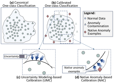
Figure 1. Demonstration of Our Key Insights. (a) Broadly-used canonical one-class classification may learn an inaccurate, biased normality boundary due to the anomaly contamination problem and the absence of knowledge about anomalies of interest. (b) By contrast, the two proposed calibration methods, UMC and NAC, respectively address these two issues, and our calibrated one-class classifier can produce a more accurate, clearer normality boundary. (c) UMC helps exclude contaminated data from training the normality based on model uncertainty scores, while (d) NAC helps ground the normality boundary by calibrating the normality with native anomalies.

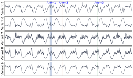
(a) Time Series Data

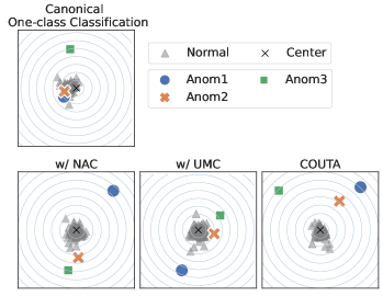
(b) Feature Space

Figure 2. (a) Time Series Data with Three Anomaly Segments; (b) Learned Feature Space of Canonical (non-calibrated) One-class Classification and Our Methods (using one or two calibration methods). Normal data is expected to be enclosed in a compact hypersphere, and anomalies can be successfully identified if they are distant from the center.

The Proposed Approach. To this end, this paper proposes a novel Calibrated One-class classification-based Unsupervised Time series Anomaly detection method (COUTA for short). The approach fulfills contamination-tolerant, anomaly-informed normality learning by two novel normality calibration methods, including uncertainty modeling-based calibration (UMC) and native anomaly-based calibration (NAC). In UMC, a novel calibrated one-class loss function is proposed, in which a prior (i.e., Gaussian) distribution is imposed on the one-class distances and utilized to capture the prediction uncertainties. It calibrates the one-class representations by emphasizing confident predictions while at the same time adaptively penalizing uncertain predictions. This prior is theoretically motivated by the probability density function of Gaussian distribution. In NAC, we propose three simple but effective data perturbation operations to generate native anomaly examples from original time series sub-sequences, on which a new supervised training branch is devised to further calibrate the normality to be discriminative w.r.t. anomaly-informed samples. By jointly optimizing these two components, our calibrated one-class classification model is enforced to be robust to anomaly contamination and discriminative to diverse types of anomaly behaviors, thus producing a more accurate data normality boundary, as depicted in Figure 1 (b).

As an example, we use the Omi-4 server data of the Application Server Dataset (ASD) (Li et al., 2021c) to have a straightforward demonstration of the benefit of each calibration to our model in Figure 2, where Figure 2 (a) visualizes the time series data (five representative variants out of the original 19 dimensions are selected) while Figure 2 (b) shows the new feature spaces learned by four different one-class classification models. It is clear that the canonical one-class classification (i.e., COUTA without calibration) fails to identify two anomalies (Anom1 and Anom2), and the hypersphere formed by normal data is also biased. By contrast, adding either NAC or UMC all effectively calibrates the normality of the data, resulting in better discrimination of real anomalies from normal data. As a result, by adding both calibrations, COUTA can easily discriminate all three anomalies of diverse abnormal behaviors.

Contributions. The contributions are summarized as follows.

• We propose the calibrated one-class classifier COUTA, which is the first anomaly detection method that simultaneously calibrates one-class classification models using prediction uncertainties and native anomalies. These two calibrations result in a contamination-tolerant, anomaly-informed COUTA.

• We propose the uncertainty modeling-based calibration, UMC. This calibration effectively restrains irregular noisy training data while at the same time enforcing the importance of regular samples that the one-class classifier can make confident predictions. This largely alleviates the negative impact of anomaly contamination.

• We propose the native anomaly-based calibration, NAC. It generates different types of realistic anomaly examples and uses them to calibrate one-class representations for learning a more precise abstraction of normality and a clearer normality boundary.

Extensive experiments show that COUTA obtains substantial detection performance improvement over 12 state-of-the-art competing methods on 6 real-world datasets (including 26 time series sequences) by 6% - 31% in $F_{1}$ score and 7% - 42% in AUC-PR. We also use synthetic time series data to show whether COUTA can well generalize to detect different anomaly types. The contribution of the two proposed calibration methods is validated in the ablation study. COUTA also has good scalability w.r.t. both length and dimensionality of time series. The impact of hyper-parameters in COUTA is also investigated.

2. Related Work

Traditional Time Series Anomaly detection.

Time series anomaly detection is an old discipline. There is a long list of traditional methods in the literature using various techniques like decomposition (Wen et al., 2019), clustering (Boniol et al., 2021), distance (Tran et al., 2020), and pattern mining (Cao et al., 2019). Besides, traditional time series prediction models such as moving average, autoregressive, and their multiple variants (Li et al., 2021a) are adapted to detect anomalies by comparing the predicted values and the real ones. Reviews of traditional time series anomaly detection can be found in (Gupta et al., 2013), and we also recommend some comprehensive time series anomaly detection benchmark studies focusing on univariate data (Paparrizos et al., 2022), multivariate data (Schmidl et al., 2022), and explainability (Jacob et al., 2021; Xu et al., 2021).

Deep Time Series Anomaly detection.

Deep learning fuels a number of deep time series anomaly detection methods. They use generative one-class learning models to restore input data or predict future data as precisely as possible. Prior work generally categorizes these current studies into reconstruction- and prediction-based methods. As the training set is dominated by normal data, reconstruction/prediction errors can indicate abnormal degrees. The core insight of these methods is to implicitly model normal patterns and behaviors via the rationale behind restoring or forecasting. The pioneer in this research line (Malhotra et al., 2016) uses Long-Short Term Memory (LSTM) network in an encoder-decoder structure. In recent years, the data mining community has made tremendous efforts to successfully enhance the performance of this pipeline by devising various advanced network structures and new reconstruction/prediction learning objectives. A number of studies focus on capturing more comprehensive temporal and inter-variant dependencies by using graph neural networks (Deng and Hooi, 2021; Zhao et al., 2020), convolutional kernels (Zhang et al., 2019; Campos et al., 2021), and variational Autoencoders (Su et al., 2019; Li et al., 2021c). Besides, adaptive memory network (Zhang et al., 2022) and hierarchical structure-based multi-resolution learning (Zhang et al., 2019; Huang et al., 2022b; Shen et al., 2020) are used to better handle diverse normal patterns. Some other methods use adversarial training in Autoencoder (Kieu et al., 2022; Audibert et al., 2020; Liu et al., 2022) or generative adversarial network (Zhao et al., 2022; Liu et al., 2022; Du et al., 2021) that introduce regularization into the learning process to alleviate the overfitting problem. Additionally, ensemble learning is also explored in (Campos et al., 2021; Kieu et al., 2019). A very recent work in VLDB (Tuli et al., 2022) employs Transformer (Vaswani et al., 2017) to effectively model long-term trends in time series data, and several tools are used as building blocks to further enhance the detection model, including adversarial training to amplify reconstruction errors, self-conditioning for better training stability and generalization, model agnostic meta-learning to handle the circumstance that only limited data are available. It is noteworthy that some studies propose new anomaly scoring strategies to replace reconstruction or prediction errors. A Transformer-based method (Xu et al., 2022b) uses association variance as a novel criterion to measure abnormality, and the literature (Feng and Tian, 2021) employs the Bayesian filtering algorithm for anomaly scoring. Various advanced techniques are equipped in this pipeline, achieving state-of-the-art performance. Nevertheless, these methods may still considerably suffer from the presence of anomaly contamination and the absence of knowledge about anomalies. We below review techniques related to solving these two key problems.

Anomaly Contamination and Label-noise Learning.

Only a few anomaly detection methods consider the anomaly contamination problem. The literature (Du et al., 2021; Pang et al., 2018, 2020) filters possible anomalous samples via self-training. An additional Autoencoder is used in (Kieu et al., 2022) to obtain a clean set of time series data before the training process. These methods attempt to use the abnormality derived from the original/additional one-class learning component to filter these noises. However, this filtering process also suffers from the anomaly contamination problem, and they may also wrongly filter some hard normal samples which are important to the network training. Therefore, these solutions may fail to well tackle this problem. This problem is also related to label-noise learning or inaccurate supervision because these hidden anomalies are essentially training data with wrong labels. This topic is under the big umbrella of the weakly-supervised paradigm. A survey (Han et al., 2020) categorizes the methodology of this research line into three perspectives, i.e., data, learning objective, and optimization policy. The proposed uncertainty modeling-based calibration in the one-class learning objective also contributes a novel solution to this research line.

Anomaly Exposure and Self-supervised Anomaly Detection.

Providing extra anomaly information is a direct solution to address the absence of knowledge about anomalies. This idea is initially proposed by a work named outlier/anomaly exposure (Hendrycks et al., 2018). This study employs data from an auxiliary natural dataset as manually introduced out-of-distribution examples. Our work is fundamentally different from (Hendrycks et al., 2018). We create dummy anomaly examples by performing data perturbation on original data instead of taking data samples from a supplementary nature dataset. Also, we focus on time series data, and (Hendrycks et al., 2018) targets at images. Creating supervision signals from data itself is an essence insight in self-supervised learning. Inspired by self-supervised research in image anomaly detection (Chai et al., 2022), some self-supervised methods are also designed for time series data. They assign class labels to different augmentation operations (e.g., adding noise, reversing, scaling, and smoothing) (Zhang et al., 2022), neural transformations (Qiu et al., 2021), contiguous and separate time segments (Deldari et al., 2021), or different time resolutions (Huang et al., 2022b). However, although these proxy tasks can help to better learn data characteristics, these tasks still fail to provide information related to anomalies. They may neglect that it is also possible to reliably simulate genuine abnormal behaviors in time series via simple data perturbation. We explore this direction in our proposed method, showing that these dummy anomaly examples can greatly benefit the learning process.

3. The Proposed COUTA

3.1. Problem Formulation

Let $\mathcal{X}=\langle\mathbf{x}_{1},\mathbf{x}_{2},\cdots,\mathbf{x}_{N}\rangle$ be a time series dataset, and $\mathcal{X}$ is an ordered sequence of $N$ observations. Each observation in $\mathcal{X}$ is a vector described by $D$ variants (i.e., $\mathbf{x}_{t}\in\mathbb{R}^{D},\forall\mathbf{x}_{t}\in\mathcal{X}$). Dataset $\mathcal{X}$ is termed as multi-variant time series when $D>1$, and the dataset is reduced to the univariate setting if $D=1$. Unsupervised time series anomaly detection $f$ is to measure the abnormal degree of each observation and give anomaly scores without accessing any label information, i.e., $f:\mathcal{X}\mapsto\mathbb{R}$. Higher anomaly scores indicate a higher likelihood to be anomalies.

We consider a local contextual window of each observation to model their temporal dependence. Specifically, a sliding window with length $l$ and stride $r$ is used to transform the training set into a collection of sub-sequences $\mathcal{S}=\{\mathbf{s}_{1},\mathbf{s}_{1+r},\cdots\}$, where $\mathbf{s}_{t}=\langle\mathbf{x}_{t},\mathbf{x}_{t+1},\cdots,\mathbf{x}_{t+l-1}\rangle$. This is a common practice in most deep time-series anomaly detection methods (Tuli et al., 2022; Campos et al., 2021; Su et al., 2019; Li et al., 2021c). During the inference stage, the testing set is also split into sub-sequences using the same window length $l$, and the sliding stride is set to 1. The anomaly detection model evaluates the abnormal degree of each sub-sequence, and the anomaly score is assigned to the last timestamp of each sub-sequence. We use 0 to pad the beginning $l-1$ timestamps to obtain the final anomaly score list.

3.2. Overall Framework

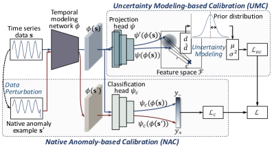
Figure 3. The Framework of COUTA.

The overall framework COUTA is shown in Figure 3. A temporal modeling network $\phi$ is used to model time-axis dependency and inter-variant interactions. We opt for Temporal Convolutional Network (TCN) (Bai et al., 2018) as the temporal modeling network $\phi$ in COUTA. TCN is more time-efficiency than traditional RNN-based structures, and it can better capture local time dependency due to the usage of convolutional kernels. We further use a lightweight projection head $\psi$ to map the data to a $H$-dimensional feature space $\mathcal{F}\subset\mathbb{R}^{H}$. The multi-layer perceptron network structure is employed in $\psi$. The whole representation process can be denoted as $\psi(\phi(\cdot))$. We aim to map the training data $\mathbf{s}$ into a compact hypersphere with center $\mathbf{c}$ upon the feature space $\mathcal{F}$. We devise the Uncertainty Modeling-based Calibration (UMC) in COUTA. Specifically, a prior probability distribution is imposed on the one-class distance. We set a bypass in $\psi$ by using an additional layer to obtain an extra prediction $\psi^{\prime}(\phi(\mathbf{s}))$, and two distance values ($d$ and $\tilde{d}$) are used to obtain the mean and the variance of the prior distribution. Our one-class learning objective $\mathcal{L}_{oc}$ is calibrated to adaptively penalize uncertain predictions and simultaneously encourage confident predictions, thus accomplishing the masking of anomaly contamination in the training set. In addition, we propose Native Anomaly-based Calibration (NAC) to introduce knowledge about time series anomalies to the one-class learning process. Native anomaly example $\mathbf{s}^{\prime}$ is created on the basis of original time series data $\mathbf{s}$ via tailored data perturbation operations. A new supervised training branch with a classification head $\psi_{c}$ is added to empower COUTA to discriminate genuine abnormal behaviors in time series via a loss function $\mathcal{L}_{c}$. We also employ the multi-layer perceptron structure in the classification head $\psi_{c}$.

The final loss function is computed by assembling:

(1) $$\mathcal{L}=\mathcal{L}_{oc}+\alpha\mathcal{L}_{c}$$

where $\alpha$ is a parameter to adjust the weight of the native anomaly-based classification training branch.

The learnable parameters within the neural network are jointly trained by loss function $\mathcal{L}$. During the inference stage, the testing set is also pre-processed to sub-sequences, and COUTA measures abnormal degrees of input sub-sequences according to their deviation from the learned normality model (i.e., the hypersphere).

3.3. Calibrated One-class Classification

3.3.1. UMC for Contamination-tolerant One-class Learning

COUTA aims at learning a hypersphere with the minimum radius that can well enclose the training data upon the feature space $\mathcal{F}$. Therefore, the data normality can be explicitly defined as this hypersphere, and the distance to the hypersphere center can faithfully indicate the degree of data abnormality.

This basic goal is the same as SVDD (Tax and Duin, 2004) (a popular technique in one-class classification). The traditional SVDD algorithm relies on the kernel trick. As has been done in a recent extension (Ruff et al., 2018), after mapping original data to a new feature space via neural network $\phi$ and $\psi$, the canonical one-class loss function can be defined as

(2) $$\mathcal{L}_{\text{canonical}}=\mathbb{E}_{\mathbf{s}\sim\mathcal{S}}\Big{[}\big{\|}\psi\big{(}\phi(\mathbf{s})\big{)}-\mathbf{c}\big{\|}^{2}\Big{]},$$

where $\mathbf{c}\in\mathbb{R}^{H}$ is the hypersphere center upon the feature space $\mathcal{F}$.

Anomaly contamination of the training set is essentially noisy data that have very rare abnormal behaviors and inconsistent patterns, and thus the one-class classification model tends to output unconfident predictions on these noisy data. Therefore, to address the anomaly contamination problem, we can give a relatively mild penalty to predictions that are with high model uncertainty, thus masking anomaly contamination in a soft manner. On the other hand, to ensure effective optimization of hard normal samples, the one-class classification model should also be encouraged to output confident predictions. The learning objective in Equation (2) is basically defined according to the distance to the hypersphere center Therefore, the core idea is to impose a prior (i.e., Gaussian) distribution $\mathcal{N}_{\mathbf{s}}(\mu,\sigma^{2})$ to the single distance value $d(\mathbf{s})=\|\psi(\phi(\mathbf{s}))-\mathbf{c}\|^{2}$, and the variance $\sigma^{2}$ of the distribution can represent the model uncertainty. Hence, to fulfill uncertainty modeling-based calibration, we need to answer two questions, i.e., how to design a new learning objective that can handle distance distribution and how to extend the single distance value to its prior distribution.

We first consider the design of our new one-class loss function. Given a prior distribution of the one-class distance, we need to maximize the probability of the distance being zero, instead of simply minimizing a single distance value. Based on the probability density function of the Gaussian distribution, the learning objective of the distance distribution $\mathcal{N}_{s}(\mu,\sigma^{2})$ of sub-sequence $\mathbf{s}$ can be defined to maximize the following function:

(3) $$J=\frac{1}{\sqrt{2\pi\sigma^{2}}}e^{-\frac{1}{2}(\frac{\mu}{\sigma})^{2}}.$$

We can further derive the following function:

(4) $$\begin{split}\log J=-\frac{1}{2\sigma^{2}}\mu^{2}-\frac{1}{2}\log\sigma^{2}.\end{split}$$

Let $\zeta=\log\sigma^{2}$, the learning objective of $\mathcal{N}_{\mathbf{s}}(\mu,\sigma^{2})$ is equivalent to minimize the following loss value:

(5) $$\ell(\mathbf{s})=\frac{1}{2}e^{-\zeta}\mu^{2}+\frac{1}{2}\zeta.$$

We then address how to extend the single output of a distance value to a Gaussian distribution. One direct solution is to employ the ensemble method to obtain a group of predictions, thus estimating the mean and the variance of the distribution. However, the GPU memory consumption and the computational effort might be costly when there are many ensemble members. The essence of the Gaussian distribution is to find the variance, that is, the ensemble process does not need a heavy computational overhead. Recall that a lightweight projection head $\psi$ is used after the temporal modeling network $\phi$, we can set a bypass hidden layer in $\psi$, thus yielding an additional projection output (denoted by $\psi^{\prime}(\phi(\mathbf{s}))$). We calculate one-class distance values of $\psi(\phi(\mathbf{s}))$ and $\psi^{\prime}(\phi(\mathbf{s}))$ as

(6) $$d=\|\psi(\phi(\mathbf{s}))-\mathbf{c}\|^{2},\tilde{d}=\|\psi^{\prime}(\phi(\mathbf{s}))-\mathbf{c}\|^{2}$$

Based on the loss value defined in Equation (5) and distance values given in Equation (6), the loss function of one-class classification with uncertainty modeling-based calibration is derived as follows.

(7) $$\mathcal{L}_{oc}=\mathbb{E}_{\mathbf{s}\sim\mathcal{S}}\Big{[}\frac{1}{2}e^{-\big{(}d(\mathbf{s})-\tilde{d}(\mathbf{s})\big{)}^{2}}\big{(}d(\mathbf{s})+\tilde{d}(\mathbf{s})\big{)}+\frac{1}{2}\big{(}d(\mathbf{s})-\tilde{d}(\mathbf{s})\big{)}^{2}\Big{]},$$

where we use $d(\mathbf{s})+\tilde{d}(\mathbf{s})$ representing $\mu^{2}$ and $(d(\mathbf{s})-\tilde{d}(\mathbf{s}))^{2}$ as $\zeta$.

Our loss function in Equation (7) successfully masks anomaly contamination by giving mild penalty loss values on these noisy data. The one-class classification model tends to output inconsistent prediction to these hidden anomalies, i.e., $|d(\mathbf{s})-\tilde{d}(\mathbf{s})|$ is high. Therefore, the loss value $d(\mathbf{s})+\tilde{d}(\mathbf{s})$ is adjusted to a lower level by its coefficient $e^{-|d(\mathbf{s})-\tilde{d}(\mathbf{s})|}$. On the other hand, the second term also penalizes high uncertainty, which encourages more confident predictions to ensure the effective optimization of hard samples. Figure 4 visualizes $\mathcal{L}_{oc}$ of Equation (7) by presenting loss values w.r.t. $d(\mathbf{s})+\tilde{d}(\mathbf{s})$ and $|d(\mathbf{s})-\tilde{d}(\mathbf{s})|$. As expected, this loss function adaptively adjusts the loss value of the data sample with high uncertainty and simultaneously impels more confident predictions.

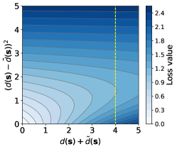
Figure 4. Loss Values in $\mathcal{L}_{oc}$ w.r.t. $d(\mathbf{s})+\tilde{d}(\mathbf{s})$ and $|d(\mathbf{s})-\tilde{d}(\mathbf{s})|$. As indicated by the yellow line, the penalty of a fixed $d(\mathbf{s})+\tilde{d}(\mathbf{s})$ is first adjusted to more mild levels with the increase of the uncertainty $|d(\mathbf{s})-\tilde{d}(\mathbf{s})|$, while the loss function further penalizes heavily when the uncertainty reaches a high value.

3.3.2. NAC for Anomaly-informed One-class Learning

To introduce knowledge about anomalies, we propose to offer dummy anomaly examples to the one-class classification model. Motivated by self-supervised learning, we introduce tailored data perturbation operations to generate native anomaly examples on the basis of original time series data.

Data perturbation $\delta$ modifies the input time series sub-sequence $\mathbf{s}$ via a specific operation to obtain a new sub-sequence $\mathbf{s}^{\prime}$ such that $\mathbf{s}^{\prime}$ contains realistic abnormal behaviors of time series. $\mathbf{s}$ and $\mathbf{s}^{\prime}$ are with the same shape. According to the definitions and characterizations of three basic time series anomaly types (i.e., point, contextual, and collective anomalies), we define the following data perturbation operations.

• $\delta_{(\text{I},\gamma)}(\mathbf{s})$: Data perturbation is performed on the last observation of the input sub-sequence $\mathbf{s}$. Data values of a group of randomly selected dimensions of the last observation are replaced with a global extreme value $\gamma$. A new sub-sequence with a point anomaly can be created.

• $\delta_{(\text{II},\gamma)}(\mathbf{s})$: Data perturbation is also applied to randomly selected dimensions of the last observation of the input sub-sequence $\mathbf{s}$. We use an offset $\gamma$ based on the mean of the previous $k$ values to pad these selected places. This perturbation method produces contextual anomalies. We use $k=10$ by default.

• $\delta_{(\text{III},\gamma)}(\mathbf{s})$: We also randomly choose a group of dimensions, but this perturbation operation acts on a segment of the input sub-sequence $\mathbf{s}$. The right side is fixed as the last observation, and the segment length is randomly sampled from the range $[1,0.2l]$. These values are replaced with an outlier value $\gamma$. This perturbation process produces collective anomalies.

In practice, each of the above operations is deployed with two $\gamma$ values to simulate anomalies at two extremes. As time series data is first preprocessed via data normalization to $[0,1]$, we use $\gamma=+2,-2$ in $\delta_{\text{I}}$, $\gamma=+0.5,-0.5$ in $\delta_{\text{II}}$, $\gamma=1,0$ in $\delta_{\text{III}}$. We define a pool $\Omega$ containing these six data perturbation functions, i.e.,

(8) $$\begin{split}\Omega=\big{\{}\delta_{(\text{I},+2)},\delta_{(\text{I},-2)},\delta_{(\text{II},+0.5)},\delta_{(\text{II},-0.5)},\delta_{(\text{III},0)},\delta_{(\text{III},1)}\big{\}}.\end{split}$$

These six perturbation functions successfully simulate genuine abnormal behaviors in time series. Figure 5 presents a base time series sub-sequence $\mathbf{s}$ and corresponding native anomaly examples generated via these six data perturbation operations within $\Omega$.

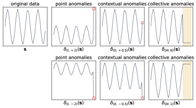
Figure 5. Native Anomaly Examples Generated from a Time Series Sub-sequence $\mathbf{s}$ by Six Perturbation Functions in $\Omega$.

A new set of dummy anomaly examples $\mathcal{S}^{\prime}$ with size $\beta|\mathcal{S}|$ is generated, which is denoted as follows.

(9) $$\mathcal{S}^{\prime}=\big{\{}\delta(\mathbf{s})|\mathbf{s}\sim\mathcal{S},\delta\sim\Omega\big{\}},$$

where original sub-sequence $\mathbf{s}$ and function $\delta$ are randomly sampled from the training set $\mathcal{S}$ and the operation pool $\Omega$.

We then set a new supervised training branch to calibrate COUTA such that our one-class classifier can discriminate primitive anomalies in $\mathcal{S}^{\prime}$. We use an extra lightweight classification head $\psi_{c}$ following the temporal modeling network $\phi$ with the multi-layer perceptron structure to map each data sample to a score. Mean Squared Error (MSE) is employed to regress the output of sub-sequences of the original set to $y_{-}$ and the output of those anomaly examples to $y_{+}$. The loss function of this branch is defined as follows.

(10) $$\mathcal{L}_{c}=\mathbb{E}_{\mathbf{s}\sim\mathcal{S}\cup\mathcal{S}^{\prime}}\Big{[}\mathbbm{1}_{\mathbf{s}\in\mathcal{S}}\big{(}\psi_{c}(\phi(\mathbf{s}))-y_{-}\big{)}^{2}+\mathbbm{1}_{\mathbf{s}\in\mathcal{S}^{\prime}}\big{(}\psi^{\prime}(\phi(\mathbf{s}))-y_{+}\big{)}^{2}\Big{]}$$

where $y_{+}=1$ and $y_{-}=-1$ are used in our implementation.

Although these manually defined perturbation operations seem to be old-school compared to deep generation methods, this way is simple enough to generate dummy anomaly examples with genuine abnormal behaviors of time series. Exposing these native anomaly examples to the one-class classification model via this training branch can lead to a more precise abstraction of data normality and a clearer boundary of the normality hypersphere.

3.4. Anomaly Scoring

The learned hypersphere upon the feature space $\mathcal{F}$ can explicitly represent the data normality, and data abnormality can be simply defined as the Euclidean distance to the hypersphere center $\mathbf{c}$. As each distance value is extended to a Gaussian distribution to express model uncertainty in our calibrated one-class classification model, we employ $\mu^{2}$ of the Gaussian distribution to define the abnormal degree. Given the optimized network including the temporal modeling network $\phi^{*}$ and the projection head ($\psi^{*}$ and $\psi^{\prime*}$), the anomaly score of a sub-sequence $\mathbf{s}$ is calculated as follows.

(11) $$\begin{split}f(\mathbf{s})&=d(\mathbf{s})+\tilde{d}(\mathbf{s})\\ &=\|\psi^{*}(\phi^{*}(\mathbf{s}))-\mathbf{c}\|+\|\psi^{\prime*}(\phi^{*}(\mathbf{s}))-\mathbf{c}\|.\end{split}$$

3.5. Discussion

Discriminative vs. Generative.

COUTA is in a discriminative manner instead of using mainstream reconstruction- or prediction-based generative models. Compared to the autoencoder structure that is composed of an encoder phase and a decoder phase, COUTA does not need to reconstruct the encoded feature back to the original shape, which is more time efficient. Moreover, COUTA learns a compact hypersphere, which is an explicit way to model data normality. That is, the optimization is directly related to anomaly detection rather than implicitly behind the rationale of data reconstruction or forecasting.

The Choice of Hypersphere Center.

Arguably, including $\mathbf{c}$ as a optimization variable will lead to a trivial solution, i.e., all learnable parameters in network $\phi$ and $\psi$ are zero (Ruff et al., 2018). Hence, following (Ruff et al., 2018), we use the initialized network to perform a forward pass on all training data, and $\mathbf{c}$ is set as the mean of the representations, i.e., $\mathbf{c}=\frac{1}{|\mathcal{S}|}\sum_{\mathbf{s}\in\mathcal{S}}\psi_{0}(\phi_{0}(\mathbf{s}))$, where $\phi_{0}$ and $\psi_{0}$ are initialized neural networks before the gradient optimization phase. It is an empirically good strategy, which makes the optimization process converge quickly and also avoids the above “hypersphere collapse” problem.

Anomaly Types in Native Anomaly Generation.

We define six perturbation functions with fixed parameters in $\Omega$. This component is also a good handle to embed readily accessible prior knowledge into the learning process. Some specific real-world applications may have their own definitions of anomalies. For example, IT operations in data centers focus on collective (pattern) anomalies and often omit point anomalies. These collective anomalies may indicate real severe faults, possible downtime of running services, and an unreasonable increase of system overhead, but point anomalies are often noises induced by many possible factors of system instability. Thus, data perturbation can be designed to generate corresponding anomalies of real interests. Note that it is also a limitation of this calibration method. These data perturbation methods are designed based on general anomaly definitions. They may bring negative effects if these generated dummy anomalies are essentially normal in target systems. Nevertheless, we empirically prove that these data perturbation methods are effective in the vast majority of real-world datasets from different domains.

Anomaly Scoring Strategy.

The anomaly scoring function does not use the prediction results reported by the classification head $\psi_{c}$. This branch is used to assist the optimization of temporal modeling network $\phi$ by providing knowledge about anomalies. We simply treat all training data as a normal class in this branch, which means this learning task might also be misled by the anomaly contamination problem. Besides, these dummy anomaly examples might not always be reliable due to the limitation analyzed above. Simply adding the output of this branch may downgrade the detection performance, and it is also challenging to devise a good ensemble method to integrate the outputs of two branches. Therefore, we leverage the one-class learning results calibrated by both UMC and NAC, i.e., the distance to the hypersphere center, to measure data abnormality in our anomaly scoring function.

4. Experiments

In this section, we first introduce the experimental setup, and then we conduct experiments to answer the following questions.

• Effectiveness: How accurate are the anomaly detection results computed by COUTA and current state-of-the-art methods on real-world datasets?

• Generalization ability: Can COUTA generalize to different types of time series anomalies?

• Robustness: How does the robustness of COUTA w.r.t. various anomaly contamination levels of the training set?

• Ablation study: Do the proposed calibration methods contribute to sufficiently better detection performance?

• Scalability: Is COUTA more time-efficient compared to existing methods?

• Sensitivity: How do hyper-parameters of COUTA influence the detection performance?

4.1. Experimental Setup

4.1.1. Datasets and Preprocessing Methods

Six publicly available datasets are used in our experiments. We introduce their background below and summarize their statistical details in Table 1.

• Application Server Dataset (ASD) contains the status (metrics related to CPU, memory, network, virtual machine, etc.) of a server collected from a large Internet company. Anomalies in this dataset are system failures and unstable factors, which are manually labeled by system operators.

• Server Machine Dataset (SMD) is also collected from a large Internet company. This dataset indicates the resource utilization of different machines in a cluster. The anomalies are labeled by domain experts according to incident reports.

• Secure Water Treatment dataset (SWaT) is collected from a water treatment testbed. The dimensions reflects values of different sensors and actuators. Anomalies are attacks that are manually launched.

• Water Quality dataset (WaQ) is released in an industrial challenge at the 2018 Genetic and Evolutionary Computation Conference (GECCO). The task is to identify true undesirable variations in the water quality according to a group of chemistry and physical metrics.

• Epilepsy seizure dataset (Epilepsy) is collected from tri-axial accelerometers on the dominant wrist. The participants are required to conduct four different activities, and we define epilepsy seizure as the anomaly class, and the other three activities including walking, running, and sawing are regarded as normal data.

• Daily and Sports Activities Dataset (DSADS) is motion sensor data of nineteen daily and sports activities collected by eight subjects. As has been done in (Zhang et al., 2022), we also use rare and intense activities (including running, ascending stairs, descending stairs, rope jumping, and playing basketball) as the anomaly class, while the remaining activities are defined as normal activities.

ASD, SMD and SWaT are broadly used as benchmark datasets in prior literature (Su et al., 2019; Li et al., 2021c; Tuli et al., 2022; Campos et al., 2021; Liu et al., 2022; Deng and Hooi, 2021). WaQ is included in a benchmark paper of time series anomaly detection (Lai et al., 2021). Epilepsy and DSADS are datasets taken from time series classification task by treating semantically abnormal class(es) as anomalies, as has been done in many prior anomaly detection studies (Xu et al., 2022a; Qiu et al., 2021; Zhang et al., 2022; Chai et al., 2020).

ASD, SMD, SWaT and WaQ have pre-defined training-testing split. In terms of Epilepsy and DSADS, we use 60% data as the training set and the remaining 40% as the testing set while maintaining the original anomaly proportion. Following (Garg et al., 2021), the minimum and maximum values per dimension of the training set are obtained to conduct min-max normalization, and the data values in the testing set are clipped to $[\min-4,\max+4]$ (i.e., the range [-4, 5]) to prevent excessively large values skewing anomaly scoring process. Deep anomaly detectors use a sliding window to divide time series datasets into small sub-sequences. Sliding window with a fixed size of 100 is used for ASD, SMD, SWaT and WaQ. We take 1 as the sliding stride for ASD and SMD and respectively use 100 and 5 for large-scale datasets SWaT and WaQ. As for the remaining two datasets, Epilepsy and DSADS, the original data format is collections of divided time sequences, and thus sliding window is not required.

Table 1. Dataset Information. $N_{\text{train}}$ and $N_{\text{test}}$ indicate the size of the training and testing set, $D$ is the dimension, #anom (ratio) denotes the anomaly size and ratio in the testing set, and #seqs is the number of time series sequences in each data repository (different sequences are trained and tested independently). For those datasets with multiple sequences, we report the average value of the above statistics.

	$N_{\text{train}}$	$N_{\text{test}}$	$D$	#anom (ratio)	#seqs
ASD	8,528	4,320	19	199 (1.5%)	12
SMD	28,703	28,703	38	270 (0.5%)	3
SWAT	475,200	449,919	51	54,584 (5.9%)	1
WaQ	138,521	115,086	11	2,329 (0.9%)	1
DSADS	85,500	57,000	47	9,000 (6.3%)	8
Epilepsy	33,784	22,866	5	5,768 (10.2%)	1

4.1.2. Competing Methods

COUTA is compared with the following twelve anomaly detection methods.

• OCSVM (Manevitz and Yousef, 2001): A classical one-class model that uses the support vector machine;

• GOAD (Bergman and Hoshen, 2020): A self-supervised anomaly detection approach that is designed for non-image data. GOAD uses random affine transformations to define its proxy task;

• ECOD (Li et al., 2022): A probability-based anomaly detection method. ECOD estimates data distribution in a non-parametric fashion, and anomalies are defined as rare events that appear in the tails of a distribution;

• LSTM-ED (Malhotra et al., 2016): A generative one-class learning (reconstruction) model that uses LSTM to construct an encoder-decoder structure. Anomalies are defined as data objects with high reconstruction errors;

• Tcn-ED (Garg et al., 2021): A generative one-class learning (reconstruction) model that uses temporal convolutional net as its encoder and decoder;

• DSVDD (Ruff et al., 2018): A discriminative one-class classification model taking deep support vector data description as its learning objective. Gate Recurrent Unit (GRU) is employed in the representation learning to handle time series data;

• MSCRED (Zhang et al., 2019): A generative one-class learning (reconstruction) method that uses the multi-scale convolutional LSTM in an encoder-decoder structure;

• Omni (Su et al., 2019): A reconstruction-based model that is basically in variational autoencoder structure. An additional component is added to capture temporal dependence;

• USAD (Audibert et al., 2020): A reconstruction-based method that uses adversely trained autoencoder. USAD employs the multi-layer perceptron (MLP) structure by reshaping windows of multi-variate time series data to a 2-D structure;

• GDN (Deng and Hooi, 2021): A prediction-based method that leverages graph attention-based forecasting. Intrinsic inter-dimension relationships can be well captured by graph neural network;

• NeuTraL (Qiu et al., 2021): A self-supervised anomaly detection model that utilizes the convolutional network. Pretext task is defined to distinguish different learnable transformations while transformed data still resemble their original form;

• TranAD (Tuli et al., 2022): A generative one-class learning (reconstruction) method that uses the Transformer network structure and model-agnostic meta-learning.

The above competitor list includes both traditional and deep approaches. Also, these competing methods employ different learning strategies (generative/discriminative one-class classification and self-supervised learning) and various network structures (MLP, LSTM, GRU, TCN, Transformer, convolutional net, and graph neural network). Therefore, the above competitor list can well represent the state-of-the-art performance of the research line of time series anomaly detection.

Table 2. $F_{1}$ score $\pm$ Standard Deviation (Precision / Recall) and AUC-PR $\pm$ Standard Deviation of COUTA and its Competing Methods on Six Real-world Datasets. MSCRED runs out of memory on SWaT.

Methods	ASD		SMD		SWaT
	$F_{1}$ ($P$/$R$)	AUC-PR	$F_{1}$ ($P$/$R$)	AUC-PR	$F_{1}$ ($P$/$R$)	AUC-PR
OCSVM	0.625±0.000 (0.801/0.602)	0.540±0.000	0.761±0.000 (0.993/0.652)	0.664±0.000	0.839±0.000 (0.975/0.737)	0.804±0.000
GOAD	0.827±0.025 (0.817/0.866)	0.834±0.023	0.975±0.019 (0.964/0.990)	0.981±0.013	0.831±0.003 (0.960/0.734)	0.799±0.005
ECOD	0.589±0.000 (0.649/0.701)	0.527±0.000	0.755±0.000 (1.000/0.637)	0.724±0.000	0.849±0.000 (0.934/0.778)	0.899±0.000
LSTM-ED	0.807±0.013 (0.849/0.812)	0.767±0.016	0.960±0.000 (0.991/0.932)	0.955±0.009	0.847±0.007 (0.925/0.781)	0.848±0.005
Tcn-ED	0.853±0.015 (0.873/0.860)	0.862±0.019	0.848±0.050 (0.857/0.885)	0.881±0.036	0.843±0.011 (0.957/0.754)	0.846±0.003
DSVDD	0.691±0.014 (0.816/0.699)	0.671±0.017	0.682±0.012 (0.934/0.599)	0.621±0.033	0.829±0.002 (0.953/0.734)	0.811±0.003
MSCRED	0.766±0.036 (0.753/0.833)	0.756±0.050	0.628±0.031 (0.987/0.481)	0.536±0.049	OOM	OOM
Omni	0.810±0.044 (0.848/0.814)	0.789±0.063	0.954±0.006 (0.981/0.930)	0.928±0.011	0.845±0.012 (0.951/0.762)	0.841±0.008
USAD	0.595±0.033 (0.825/0.563)	0.510±0.035	0.744±0.006 (0.937/0.642)	0.658±0.006	0.835±0.000 (0.964/0.737)	0.808±0.000
GDN	0.801±0.034 (0.825/0.826)	0.779±0.042	0.939±0.015 (0.917/0.969)	0.959±0.016	0.846±0.025 (0.937/0.778)	0.885±0.036
NeuTraL	0.627±0.047 (0.698/0.655)	0.592±0.045	0.770±0.050 (0.855/0.763)	0.746±0.067	0.862±0.023 (0.974/0.774)	0.850±0.026
TranAD	0.899±0.020 (0.884/0.927)	0.915±0.018	0.761±0.001 (0.995/0.650)	0.662±0.003	0.831±0.009 (0.962/0.732)	0.810±0.007
COUTA	0.942±0.031 (0.917/0.972)	0.955±0.030	0.980±0.018 (0.964/0.998)	0.984±0.015	0.886±0.022 (0.910/0.866)	0.900±0.017
Methods	WaQ		DSADS		Epilepsy
	$F_{1}$ (P/R)	AUC-PR	$F_{1}$ (P/R)	AUC-PR	$F_{1}$ (P/R)	AUC-PR
OCSVM	0.732±0.000 (0.807/0.669)	0.666±0.000	0.807±0.000 (0.700/0.972)	0.753±0.000	0.781±0.000 (0.717/0.857)	0.708±0.000
GOAD	0.739±0.052 (0.931/0.614)	0.685±0.034	0.723±0.014 (0.725/0.734)	0.676±0.015	0.554±0.147 (0.690/0.700)	0.530±0.128
ECOD	0.676±0.000 (0.802/0.584)	0.716±0.000	0.923±0.000 (0.883/0.971)	0.941±0.000	0.785±0.000 (0.751/0.821)	0.763±0.000
LSTM-ED	0.759±0.006 (0.850/0.687)	0.714±0.018	0.865±0.011 (0.805/0.943)	0.902±0.005	0.802±0.012 (0.750/0.864)	0.784±0.012
Tcn-ED	0.707±0.082 (0.839/0.632)	0.658±0.090	0.850±0.021 (0.868/0.864)	0.868±0.023	0.758±0.011 (0.740/0.793)	0.763±0.008
DSVDD	0.519±0.038 (0.911/0.368)	0.410±0.043	0.751±0.057 (0.706/0.820)	0.690±0.078	0.686±0.040 (0.578/0.850)	0.555±0.069
MSCRED	0.717±0.007 (0.945/0.578)	0.644±0.016	0.657±0.029 (0.622/0.712)	0.659±0.062	0.640±0.017 (0.579/0.736)	0.604±0.023
Omni	0.738±0.018 (0.828/0.668)	0.714±0.023	0.867±0.018 (0.895/0.853)	0.914±0.015	0.811±0.027 (0.756/0.879)	0.780±0.054
USAD	0.666±0.049 (0.771/0.603)	0.611±0.044	0.733±0.041 (0.673/0.846)	0.713±0.065	0.663±0.009 (0.538/0.864)	0.541±0.038
GDN	0.640±0.052 (0.635/0.683)	0.659±0.043	0.795±0.022 (0.747/0.879)	0.728±0.024	0.783±0.010 (0.728/0.850)	0.789±0.010
NeuTraL	0.681±0.085 (0.874/0.582)	0.616±0.111	0.534±0.035 (0.409/0.794)	0.490±0.045	0.739±0.075 (0.658/0.857)	0.729±0.111
TranAD	0.755±0.010 (0.912/0.644)	0.729±0.017	0.730±0.114 (0.745/0.767)	0.690±0.158	0.776±0.008 (0.680/0.907)	0.734±0.012
COUTA	0.781±0.013 (0.939/0.670)	0.714±0.006	0.926±0.029 (0.894/0.962)	0.942±0.020	0.830±0.053 (0.758/0.921)	0.823±0.086

4.1.3. Evaluation Metrics and Computing Infrastructure

Many anomalies in time series data are consecutive, and they can be viewed as multiple anomaly segments. In many practical applications, an anomaly segment can be properly handled if detection models can trigger an alert at any timestamp within this segment. Therefore, the vast majority of previous studies (Su et al., 2019; Li et al., 2021c; Tuli et al., 2022; Audibert et al., 2020; Liu et al., 2022; Deng and Hooi, 2021; Xu et al., 2022b) employ point-adjust strategy in their experiment protocols. Specifically, the scores of observations in each anomaly segment are adjusted to the highest value within this segment, which simulates the above assumption (a single alert is sufficient to take action). Other points outside anomaly segments are treated as usual. For the sake of consistency with current literature, we also employ this adjustment strategy before computing evaluation metrics.

Precision $P$ and recall $R$ of the anomaly class can directly indicate costs and benefits of finding anomalies in real-world applications, which can intuitively reflect model performance. $F_{1}$ score is the harmonic mean of precision and recall, which takes both precision and recall into account. These detection models output continuous anomaly scores, but there is often no specific way to determine a decision threshold when calculating precision and recall. Therefore, following prior work in this research line (Su et al., 2019; Li et al., 2021c; Tuli et al., 2022; Campos et al., 2021; Liu et al., 2022; Audibert et al., 2020), we use the best $F_{1}$ score and the Area Under the Precision-Recall Curve (AUC-PR), considering simplicity and fairness. These two metrics can avoid possible bias brought by fixed thresholds or threshold calculation methods. The best $F_{1}$ score represents the optimal case, while AUC-PR is in an average case that is less optimal. Specifically, we enumerate all possible thresholds (i.e., scores of each timestamp) and compute corresponding precision and recall scores. The best $F_{1}$ can then be obtained, and AUC-PR is computed by employing the average precision score. In the following experiments, we use $F_{1}$, $P$, and $R$ denote the best $F_{1}$ and its corresponding precision and recall score. The above performance evaluation metrics range from 0 to 1, and a higher value indicates better performance.

All the experiments are executed at a workstation with an Intel(R) Xeon(R) Silver 4210R CPU @ 2.4GHz, an NVIDIA TITAN RTX GPU, and 64 GB RAM.

4.1.4. Parameter Settings and Implementations

In COUTA, the temporal modeling network $\phi$ is with one hidden layer, and the kernel size uses 2. The projection head $\psi$ and the classification head $\psi_{c}$ are two-layer multi-layer perceptron networks with LeakyReLU activation. The hidden layer of $\phi$ and $\psi$ has 16 neural units by default, and the dimension of the feature space $\mathcal{F}$ is also 16. We respectively use 32 and 64 in complicated dataset ASD and DSADS to enhance the representation power of the neural network. Adam optimizer is employed, where the learning rate is set to $10^{-4}$. COUTA is trained with 40 epochs on datasets ASD, WaQ, DSADS, and other three datasets use 20 epochs. We use 64 data objects per training mini-batch. The weight factor $\alpha$ of the supervised classification branch in the loss function uses 0.1 by default. The factor $\beta$ that controls the size of generated anomaly examples is set to 0.2. As for our competitors, we use the default or recommended hyper-parameter settings in their respective original papers.

These anomaly detectors are implemented in Python. We use the implementations of OCSVM and ECOD from pyod, a python library of anomaly detection approaches. The source code of GOAD, DSVDD, USAD, GDN, NeuTraL, and TranAD are released by their original authors. In terms of LSTM-ED, Tcn-ED, MSCRED, and Omni, we use the implementations from an evaluation study (Garg et al., 2021).

4.2. Effectiveness in Real-World Datasets

This experiment evaluates the effectiveness of COUTA. We perform COUTA and its twelve competing methods on six real-world time series datasets. These models are trained on training sets, and we report their detection performance on testing sets. Ground-truth labels in testing sets are strictly unknown in the training stage.

Table 2 illustrates the $F_{1}$ score, AUC-PR, and corresponding standard deviation of thirteen time series anomaly detectors. MSCRED runs out of memory on the large-scale dataset SWaT due to the high computational cost of the deep convolutional network structure used in MSCRED. COUTA obtains the best $F_{1}$ performance among thirteen detectors on all datasets. In terms of AUC-PR, COUTA outperforms all of its state-of-the-art competing methods on five datasets with a 0.015 disparity to the best performer on the remaining one dataset. Averagely, COUTA achieves 6.1% - 30.7 % $F_{1}$ improvement and 7.0% - 41.5 % AUC-PR enhancement over its twelve state-of-the-art competitors.

TranAD and GDN achieve relatively good detection performance compared to other models. TranAD employs the advanced Transformer structure and several training tricks, and GDN models inter-variant correlations with the help of the powerful capability of graph neural networks in exploring high-order interactions among graph nodes. However, TranAD may suffer from the overfitting problem because its learning process is with several complicated components, and thus it fails to produce effective detection results on simple datasets like SMD and SWaT. In contrast, detectors with plain encoder-decoder structures (e.g., LSTM-ED) obtain better performance. The canonical one-class learning process used in these competing methods suffers from noisy training samples (i.e., anomaly contamination), and they may also learn an inaccurate range of normal behaviors due to the lack of guidance about the anomaly class. It is noteworthy that, on dataset SWaT, a pure training set with only normal observations is ensured (water treatment attack is only launched in the testing set), and thus these competing methods can obtain relatively good performance. According to the comparison results, our method COUTA successfully achieves state-of-the-art performance. The superiority of COUTA can attribute to the synergy of our two novel one-class calibration components, which achieves contamination-tolerant, anomaly-informed learning of data normality. COUTA turns to address two key limitations in the current one-class learning pipeline rather than a more advanced network structure that is intensively studied.

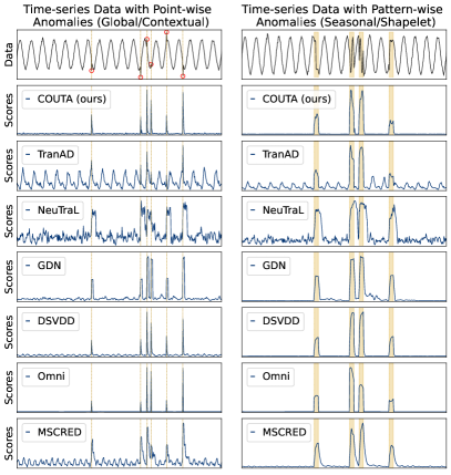
Figure 6. Performance of Detecting Point-wise (Global and Contextual) Anomalies and Pattern-wise (Seasonal and Shapelet) Anomalies in Synthetic Time Series Datasets.

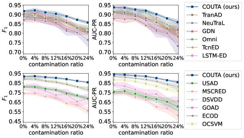
(a) Epilepsy

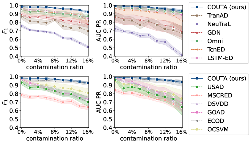
(b) DSADS

Figure 7. Robustness w.r.t. Anomaly Contamination. Twelve contenders of COUTA are separated into two groups for the sake of clarity.

4.3. Generalization Ability to Different Types of Time Series Anomalies

We investigate whether COUTA successfully handles different anomaly types in time series data. Following a fine-grained taxonomy of time series anomalies in (Lai et al., 2021), two synthetic datasets are created, in which we add point-wise anomalies and pattern-wise anomalies, respectively. Point-wise anomalies include both global and contextual forms, and pattern-wise anomalies are caused by basic shapelet and seasonality changes. We do not consider trend anomalies in this experiment because simple threshold alarming can be used to identify trend alternations. This experiment focuses on the comparison of state-of-the-art deep time series anomaly detection methods, and we omit anomaly detectors that are in plain encoder-decoder structure or are not designed for time series.

Figure 6 illustrates these two synthetic datasets (the top panel) and the anomaly scores produced by our method COUTA and competing methods. Intuitively, one-class learning-based detectors can generalize well to different anomaly types because these models can alarm all the observations that are deviated from the learned normality. Therefore, these anomaly detectors can give higher scores to real abnormal points or segments. However, some competing methods produce fluctuated anomaly scores that may mislead human analysts. In contrast, COUTA successfully identifies all of these anomaly cases with distinguishably higher scores on true anomalies and low scores on normal moments. Note that these methods can effectively handle the second dataset with more challenging pattern anomalies, it might be because temporal dependency is well modeled by deep network structures.

4.4. Robustness w.r.t. Anomaly Contamination

This experiment is to quantitatively measure the interference of anomaly contamination to time series anomaly detectors, that is, we test the robustness of each anomaly detector w.r.t. different anomaly contamination ratios of the training set. Due to the continuity of time series data, we cannot directly remove or inject anomalies like other robustness testing experiments in prior work on tabular data (Pang et al., 2019). It is hard to precisely adjust ratios of abnormal timestamps in the training set. Therefore, we employ datasets Epilepsy and DSADS in this experiment because these datasets are collections of divided small sequences with sequence-level labels. We treat small sequences as data objects and generate a group of datasets with different anomaly contamination levels of the training set. We first randomly remove anomaly sequences in the training set to meet the requirements of specific contamination ratios. The removed anomalies are then added to the testing set. The original sequence-level anomaly contamination rate in Epilepsy and DSADS are 24% and 16%, respectively. A wide range of contamination levels is used for each dataset by starting from a pure training set and taking 4% as the increasing step.

Figure 7 presents the $F_{1}$ score and the AUC-PR performance of COUTA and its twelve competing methods on datasets with different anomaly contamination ratios. The performance of all anomaly detectors downgrades with the increase of anomaly contamination. COUTA shows better robustness compared to its twelve contenders, especially on datasets with a large contamination rate. It owes to the novel one-class classification loss function, which successfully masks these noisy data via uncertainty modeling-based adaptive penalty. By contrast, these competing methods simply view these hidden anomalies as normal data, and the learned normality model may mistakenly overfit these noises. This experiment validates the contribution of the proposed uncertainty modeling-based calibration method. This experiment also shows superior applicability of COUTA in some real-world applications that are with complicated noisy circumstances.

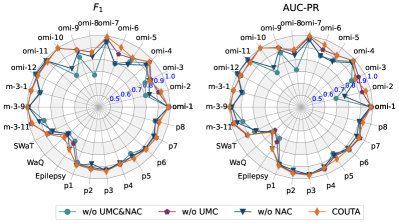
Figure 8. Ablation Study Results. Each vertex represents a single time series sequence in datasets used in the experiments, i.e., datasets with multiple sequences are shown in different vertexes. Sequences omi-1 to omi-12 are servers in dataset ASD, m-3-1, m-3-9, and m-3-11 are three machines in SMD, and sequences of patients p1 to p8 are from DSADS.

4.5. Ablation Study

This experiment further validates the contribution of two key components in COUTA. Three ablated variants are used. Two calibration methods, i.e., uncertainty modeling-based calibration and native anomaly-based calibration, are respectively removed from COUTA in two ablated variants, w/o UMC and w/o NAC. These two components are simultaneously excluded in w/o UMC&NAC. The remaining parts of these ablated versions remain the same as COUTA.

We report the $F_{1}$ and AUC-PR performance of standard COUTA and its three ablated versions in Figure 8. To better illustrate the difference between these ablation variants and COUTA, we use a radar plot where each vertex is a single time series sequence in the used datasets. Based on the comparison of COUTA and its variants, the superiority of COUTA on the vast majority of 26 sequences from six real-world datasets can verify the significant contribution of two calibration methods on one-class classification. Besides, compared to the canonical one-class classifier (i.e., w/o UMC&NAC), UMC and NAC respectively obtain 2.4% and 4.4% average improvement over these six datasets. Particularly, UMC conduces to over 11% improvement in $F_{1}$ score and approximate 15% gain in AUC-PR on the Epilepsy dataset, where the training set is severely contaminated by unknown anomalies, and NAC can bring over 8 % enhancement in both $F_{1}$ and AUC-PR on the ASD dataset.

4.6. Scalability Test

This experiment investigates the scalability of COUTA compared to its competing methods. Time efficiency w.r.t. both time series length $T$ and dimensionality $D$ are recorded. As for the scalability test w.r.t. dimensionality, A group of seven time-series datasets with a fixed length (i.e., 2000) and various dimensions (i.e., from 8 to 512 with 2 as the magnification factor) is generated. We synthesize another group of nine datasets containing different lengths (i.e., range from 1,000 to 256,000) and a fixed dimension (i.e., 8) for the scale-up test w.r.t. time series length. As these deep anomaly detectors are deployed with different numbers of training epochs, we report the execution time of one training epoch by taking 128 as a unified size of training mini-batches.

Figure 9 presents the execution time of COUTA and its ten competing state-of-the-art methods on time series datasets with various sizes. Note that this experiment excludes three anomaly detectors (i.e., OCSVM, ECOD, and GOAD) that are not originally designed for time series data. COUTA has outstanding scalability compared to existing work, which shows its potential capability of being applied in practical scenarios where time series data are with large volumes and high dimensions.

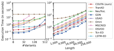
Figure 9. Scalability Test Results w.r.t. the Number of Variants and the Length of Time Series. TranAD, USAD, and MSCRED runs out of memory when handling time series data with higher dimensions.

4.7. Sensitivity Test

This experiment shows the impact of different parameter settings on detection performance. First, we only use a single kind of perturbation ($\delta_{I}$ , $\delta_{II}$, or $\delta_{III}$) to solely generate point, contextual, or collective anomalies in NAC. Besides, we investigate several key hyper-parameters of COUTA including $\alpha$, $\beta$, $H$, and $l$. $\alpha$ is the weight of loss $\mathcal{L}_{c}$ in Equation (1), $\beta$ is the ratio that controls the size of generated anomaly examples, $H$ is the dimensionality of the feature space $\mathcal{F}$, and $l$ is the sliding window length. Each parameter is sampled from a wide range.

Figure 10 shows the $F_{1}$ performance of COUTA by taking different parameter settings, and AUC-PR performance also shows the same trend, which is omitted here. COUTA shows better performance when a full perturbation operation pool $\Omega$ is employed in NAC (especially on the ASD dataset). A single type of generated anomaly example may provide fragmentary knowledge about the anomaly class, thus leading to less optimal detection performance. In terms of $\alpha$, $\beta$, and $l$, these parameters do not largely influence the performance, and COUTA performs stably with different hyper-parameters. Some parameter selection methods can be employed. Given that there might be some unreliable generated anomaly examples that fall into the normal distribution, and thus we use $\alpha=0.1$, $\beta=0.2$ by default. In terms of $l$, we employ a frequently-used sliding window length (i.e., $l=100$). COUTA shows fluctuation trends w.r.t. the dimensionality of the feature space $H$. It might be because these time series datasets are with various numbers of variants. Thus, we set different $H$ for these real-world datasets.

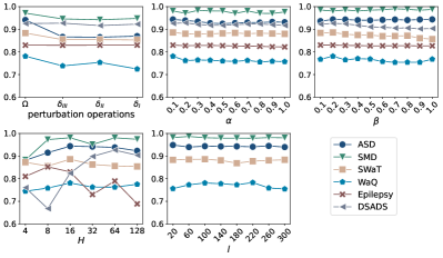
Figure 10. Sensitivity Test Results ($F_{1}$ performance w.r.t. different parameter settings). Epilepsy and DSADS have default length of sub-sequences, and thus the detection performance w.r.t. $l$ on these two datasets is omitted.

5. Conclusions

This paper introduces COUTA, an unsupervised time series anomaly detection method based on calibrated one-class classification. Instead of devising advanced network structures or new reconstruction/prediction learning objectives, we address two key limitations in the current one-class learning pipeline, i.e., the presence of anomaly contamination and the absence of knowledge about anomalies. COUTA achieves this by two novel calibration methods – uncertainty modeling-based calibration (UMC) and native anomaly-based calibration (NAC). In UMC, we obtain model uncertainty by imposing a prior distribution to the one-class distance value, and a theoretically motivated novel learning objective is devised to mildly penalize noisy data that are with high uncertainty and simultaneously encourage more confident predictions to ensure effective learning of hard normal samples. In NAC, we design tailored data perturbation operations to produce native anomaly examples on the basis of original time series data, which provides one-class classification with valuable knowledge about genuine abnormal behaviors in a very simple manner. These calibration methods enable COUTA to learn data normality in a noise-tolerant, anomaly-informed manner. Extensive experiments show that COUTA achieves state-of-the-art performance in time series anomaly detection by substantially outperforming twelve existing competitors. We also validate several desired properties of COUTA, including outstanding generalization ability to different anomaly types, superior robustness w.r.t. anomaly contamination, and good scalability.

References

- (1)
- Audibert et al. (2020) Julien Audibert, Pietro Michiardi, Frédéric Guyard, Sébastien Marti, and Maria A Zuluaga. 2020. USAD: unsupervised anomaly detection on multivariate time series. In KDD. 3395–3404.
- Bai et al. (2018) Shaojie Bai, J Zico Kolter, and Vladlen Koltun. 2018. An empirical evaluation of generic convolutional and recurrent networks for sequence modeling. arXiv preprint arXiv:1803.01271 (2018).
- Bergman and Hoshen (2020) Liron Bergman and Yedid Hoshen. 2020. Classification-Based Anomaly Detection for General Data. In ICLR.
- Boniol et al. (2021) Paul Boniol, John Paparrizos, Themis Palpanas, and Michael J Franklin. 2021. SAND: streaming subsequence anomaly detection. Proceedings of the VLDB Endowment 14, 10 (2021), 1717–1729.
- Campos et al. (2021) David Campos, Tung Kieu, Chenjuan Guo, Feiteng Huang, Kai Zheng, Bin Yang, and Christian S Jensen. 2021. Unsupervised time series outlier detection with diversity-driven convolutional ensembles. Proceedings of the VLDB Endowment 15, 3 (2021), 611–623.
- Cao et al. (2019) Lei Cao, Yizhou Yan, Samuel Madden, Elke A Rundensteiner, and Mathan Gopalsamy. 2019. Efficient discovery of sequence outlier patterns. Proceedings of the VLDB Endowment 12, 8 (2019), 920–932.
- Chai et al. (2020) Chengliang Chai, Lei Cao, Guoliang Li, Jian Li, Yuyu Luo, and Samuel Madden. 2020. Human-in-the-loop outlier detection. In SIGMOD. 19–33.
- Chai et al. (2022) Heyan Chai, Weijun Su, Siyu Tang, Ye Ding, Binxing Fang, and Qing Liao. 2022. Improving Anomaly Detection with a Self-Supervised Task Based on Generative Adversarial Network. In ICASSP. IEEE, 3563–3567.
- Deldari et al. (2021) Shohreh Deldari, Daniel V Smith, Hao Xue, and Flora D Salim. 2021. Time series change point detection with self-supervised contrastive predictive coding. In WWW. 3124–3135.
- Deng and Hooi (2021) Ailin Deng and Bryan Hooi. 2021. Graph neural network-based anomaly detection in multivariate time series. In AAAI, Vol. 35. 4027–4035.
- Du et al. (2021) Bowen Du, Xuanxuan Sun, Junchen Ye, Ke Cheng, Jingyuan Wang, and Leilei Sun. 2021. GAN-Based Anomaly Detection for Multivariate Time Series Using Polluted Training Set. IEEE Transactions on Knowledge and Data Engineering (2021).
- Feng and Tian (2021) Cheng Feng and Pengwei Tian. 2021. Time series anomaly detection for cyber-physical systems via neural system identification and bayesian filtering. In KDD. 2858–2867.
- Garg et al. (2021) Astha Garg, Wenyu Zhang, Jules Samaran, Ramasamy Savitha, and Chuan-Sheng Foo. 2021. An Evaluation of Anomaly Detection and Diagnosis in Multivariate Time Series. IEEE Transactions on Neural Networks and Learning Systems (2021).
- Golan and El-Yaniv (2018) Izhak Golan and Ran El-Yaniv. 2018. Deep anomaly detection using geometric transformations. In NeuraIPS. 9781–9791.
- Gupta et al. (2013) Manish Gupta, Jing Gao, Charu C Aggarwal, and Jiawei Han. 2013. Outlier detection for temporal data: A survey. IEEE Transactions on Knowledge and data Engineering 26, 9 (2013), 2250–2267.
- Han et al. (2020) Bo Han, Quanming Yao, Tongliang Liu, Gang Niu, Ivor W Tsang, James T Kwok, and Masashi Sugiyama. 2020. A survey of label-noise representation learning: Past, present and future. arXiv preprint arXiv:2011.04406 (2020).
- Hendrycks et al. (2018) Dan Hendrycks, Mantas Mazeika, and Thomas Dietterich. 2018. Deep Anomaly Detection with Outlier Exposure. In ICLR.
- Huang et al. (2022b) Desen Huang, Lifeng Shen, Zhongzhong Yu, Zhenjing Zheng, Min Huang, and Qianli Ma. 2022b. Efficient time series anomaly detection by multiresolution self-supervised discriminative network. Neurocomputing 491 (2022), 261–272.
- Huang et al. (2022a) Tao Huang, Pengfei Chen, and Ruipeng Li. 2022a. A Semi-Supervised VAE Based Active Anomaly Detection Framework in Multivariate Time Series for Online Systems. In WWW. 1797–1806.
- Hundman et al. (2018) Kyle Hundman, Valentino Constantinou, Christopher Laporte, Ian Colwell, and Tom Soderstrom. 2018. Detecting spacecraft anomalies using lstms and nonparametric dynamic thresholding. In KDD. 387–395.
- Jacob et al. (2021) Vincent Jacob, Fei Song, Arnaud Stiegler, Bijan Rad, Yanlei Diao, and Nesime Tatbul. 2021. Exathlon: a benchmark for explainable anomaly detection over time series. Proceedings of the VLDB Endowment 14, 11 (2021), 2613–2626.
- Kieu et al. (2019) Tung Kieu, Bin Yang, Chenjuan Guo, and Christian S Jensen. 2019. Outlier Detection for Time Series with Recurrent Autoencoder Ensembles. In IJCAI. 2725–2732.
- Kieu et al. (2022) Tung Kieu, Bin Yang, Chenjuan Guo, Christian S Jensen, Yan Zhao, Feiteng Huang, and Kai Zheng. 2022. Robust and Explainable Autoencoders for Unsupervised Time Series Outlier Detection—Extended Version. arXiv preprint arXiv:2204.03341 (2022).
- Lai et al. (2021) Kwei-Herng Lai, Daochen Zha, Junjie Xu, Yue Zhao, Guanchu Wang, and Xia Hu. 2021. Revisiting time series outlier detection: Definitions and benchmarks. In NeuraIPS (Datasets and Benchmarks Track).
- Li et al. (2021b) Chun-Liang Li, Kihyuk Sohn, Jinsung Yoon, and Tomas Pfister. 2021b. Cutpaste: Self-supervised learning for anomaly detection and localization. In CVPR. 9664–9674.
- Li et al. (2021a) Jia Li, Shimin Di, Yanyan Shen, and Lei Chen. 2021a. FluxEV: a fast and effective unsupervised framework for time-series anomaly detection. In WSDM. 824–832.
- Li et al. (2021c) Zhihan Li, Youjian Zhao, Jiaqi Han, Ya Su, Rui Jiao, Xidao Wen, and Dan Pei. 2021c. Multivariate time series anomaly detection and interpretation using hierarchical inter-metric and temporal embedding. In KDD. 3220–3230.
- Li et al. (2022) Zheng Li, Yue Zhao, Xiyang Hu, Nicola Botta, Cezar Ionescu, and George H Chen. 2022. ECOD: Unsupervised Outlier Detection Using Empirical Cumulative Distribution Functions. arXiv preprint arXiv:2201.00382 (2022).
- Liu et al. (2021) Ning Liu, Songlei Jian, Dongsheng Li, Yiming Zhang, Zhiquan Lai, and Hongzuo Xu. 2021. Hierarchical adaptive pooling by capturing high-order dependency for graph representation learning. IEEE Transactions on Knowledge and Data Engineering (2021).
- Liu et al. (2022) Shenghua Liu, Bin Zhou, Quan Ding, Bryan Hooi, Zheng bo Zhang, Huawei Shen, and Xueqi Cheng. 2022. Time series anomaly detection with adversarial reconstruction networks. IEEE Transactions on Knowledge and Data Engineering (2022).
- Malhotra et al. (2016) Pankaj Malhotra, Anusha Ramakrishnan, Gaurangi Anand, Lovekesh Vig, Puneet Agarwal, and Gautam Shroff. 2016. LSTM-based encoder-decoder for multi-sensor anomaly detection. arXiv preprint arXiv:1607.00148 (2016).
- Manevitz and Yousef (2001) Larry M Manevitz and Malik Yousef. 2001. One-class SVMs for document classification. Journal of machine Learning research 2, Dec (2001), 139–154.
- Pang et al. (2018) Guansong Pang, Longbing Cao, Ling Chen, and Huan Liu. 2018. Learning representations of ultrahigh-dimensional data for random distance-based outlier detection. In KDD. 2041–2050.
- Pang et al. (2021) Guansong Pang, Chunhua Shen, Longbing Cao, and Anton Van Den Hengel. 2021. Deep learning for anomaly detection: A review. ACM Computing Surveys (CSUR) 54, 2 (2021), 1–38.
- Pang et al. (2019) Guansong Pang, Chunhua Shen, and Anton van den Hengel. 2019. Deep anomaly detection with deviation networks. In KDD. 353–362.
- Pang et al. (2020) Guansong Pang, Cheng Yan, Chunhua Shen, Anton van den Hengel, and Xiao Bai. 2020. Self-trained deep ordinal regression for end-to-end video anomaly detection. In CVPR. 12173–12182.
- Paparrizos et al. (2022) John Paparrizos, Yuhao Kang, Paul Boniol, Ruey S Tsay, Themis Palpanas, and Michael J Franklin. 2022. TSB-UAD: an end-to-end benchmark suite for univariate time-series anomaly detection. Proceedings of the VLDB Endowment 15, 8 (2022), 1697–1711.
- Qiu et al. (2021) Chen Qiu, Timo Pfrommer, Marius Kloft, Stephan Mandt, and Maja Rudolph. 2021. Neural transformation learning for deep anomaly detection beyond images. In ICML. PMLR, 8703–8714.
- Ruff et al. (2018) Lukas Ruff, Robert A Vandermeulen, Nico Görnitz, Lucas Deecke, Shoaib A Siddiqui, Alexander Binder, Emmanuel Müller, and Marius Kloft. 2018. Deep One-Class Classification. In ICML. PMLR, 4393–4402.
- Schmidl et al. (2022) Sebastian Schmidl, Phillip Wenig, and Thorsten Papenbrock. 2022. Anomaly Detection in Time Series: A Comprehensive Evaluation. Proceedings of the VLDB Endowment 15, 9 (2022), 1779–1797.
- Shen et al. (2020) Lifeng Shen, Zhuocong Li, and James Kwok. 2020. Timeseries anomaly detection using temporal hierarchical one-class network. NeuraIPS 33 (2020), 13016–13026.
- Su et al. (2019) Ya Su, Youjian Zhao, Chenhao Niu, Rong Liu, Wei Sun, and Dan Pei. 2019. Robust anomaly detection for multivariate time series through stochastic recurrent neural network. In KDD. 2828–2837.
- Tax and Duin (2004) David MJ Tax and Robert PW Duin. 2004. Support vector data description. Machine learning 54, 1 (2004), 45–66.
- Tran et al. (2020) Luan Tran, Min Y Mun, and Cyrus Shahabi. 2020. Real-time distance-based outlier detection in data streams. Proceedings of the VLDB Endowment 14, 2 (2020), 141–153.
- Tuli et al. (2022) Shreshth Tuli, Giuliano Casale, and Nicholas R Jennings. 2022. TranAD: Deep Transformer Networks for Anomaly Detection in Multivariate Time Series Data. VLDB 15, 6 (2022), 1201–1214.
- Vaswani et al. (2017) Ashish Vaswani, Noam Shazeer, Niki Parmar, Jakob Uszkoreit, Llion Jones, Aidan N Gomez, Ł ukasz Kaiser, and Illia Polosukhin. 2017. Attention is All you Need. In NeuraIPS, Vol. 30. Curran Associates, Inc.
- Wen et al. (2019) Qingsong Wen, Jingkun Gao, Xiaomin Song, Liang Sun, Huan Xu, and Shenghuo Zhu. 2019. RobustSTL: A robust seasonal-trend decomposition algorithm for long time series. In AAAI, Vol. 33. 5409–5416.
- Wu and Keogh (2021) Renjie Wu and Eamonn Keogh. 2021. Current time series anomaly detection benchmarks are flawed and are creating the illusion of progress. IEEE Transactions on Knowledge and Data Engineering (2021).
- Wu et al. (2021) Zhiyue Wu, Hongzuo Xu, Guansong Pang, Fengyuan Yu, Yijie Wang, Songlei Jian, and Yongjun Wang. 2021. Dram failure prediction in aiops: Empirical evaluation, challenges and opportunities. arXiv preprint arXiv:2104.15052 (2021).
- Xu et al. (2022a) Hongzuo Xu, Guansong Pang, Yijie Wang, and Yongjun Wang. 2022a. Deep Isolation Forest for Anomaly Detection. arXiv preprint arXiv:2206.06602 (2022).
- Xu et al. (2021) Hongzuo Xu, Yijie Wang, Songlei Jian, Zhenyu Huang, Yongjun Wang, Ning Liu, and Fei Li. 2021. Beyond outlier detection: Outlier interpretation by attention-guided triplet deviation network. In WWW. 1328–1339.
- Xu et al. (2022b) Jiehui Xu, Haixu Wu, Jianmin Wang, and Mingsheng Long. 2022b. Anomaly Transformer: Time Series Anomaly Detection with Association Discrepancy. In ICLR.
- Zhang et al. (2019) Chuxu Zhang, Dongjin Song, Yuncong Chen, Xinyang Feng, Cristian Lumezanu, Wei Cheng, Jingchao Ni, Bo Zong, Haifeng Chen, and Nitesh V Chawla. 2019. A deep neural network for unsupervised anomaly detection and diagnosis in multivariate time series data. In AAAI, Vol. 33. 1409–1416.
- Zhang et al. (2022) Yuxin Zhang, Jindong Wang, Yiqiang Chen, Han Yu, and Tao Qin. 2022. Adaptive memory networks with self-supervised learning for unsupervised anomaly detection. IEEE Transactions on Knowledge and Data Engineering (2022).
- Zhao et al. (2020) Hang Zhao, Yujing Wang, Juanyong Duan, Congrui Huang, Defu Cao, Yunhai Tong, Bixiong Xu, Jing Bai, Jie Tong, and Qi Zhang. 2020. Multivariate time-series anomaly detection via graph attention network. In ICDM. IEEE, 841–850.
- Zhao et al. (2022) Yan Zhao, Xuanhao Chen, Liwei Deng, Tung Kieu, Chenjuan Guo, Bin Yang, Kai Zheng, and Christian S Jensen. 2022. Outlier detection for streaming task assignment in crowdsourcing. In WWW. 1933–1943.