Finite-sample bias-correction factors for the median absolute deviation based on the Harrell-Davis quantile estimator and its trimmed modification

Abstract

The median absolute deviation is a widely used robust measure of statistical dispersion. Using a scale constant, we can use it as an asymptotically consistent estimator for the standard deviation under normality. For finite samples, the scale constant should be corrected in order to obtain an unbiased estimator. The bias-correction factor depends on the sample size and the median estimator. When we use the traditional sample median, the factor values are well known, but this approach does not provide optimal statistical efficiency. In this paper, we present the bias-correction factors for the median absolute deviation based on the Harrell-Davis quantile estimator and its trimmed modification which allow us to achieve better statistical efficiency of the standard deviation estimations. The obtained estimators are especially useful for samples with a small number of elements.

Keywords: median absolute deviation, bias correction, Harrell-Davis quantile estimator, robustness.

1 Introduction

We consider the median absolute deviation as a robust alternative to the standard deviation. In order to make it asymptotically consistent with the standard deviation under the normal distribution, the median absolute deviation should be multiplied by a scale constant $C_{\infty}\approx 1.4826$. This approach works well in practice when the sample size $n$ is large. However, when the sample size is small, the usage of $C_{\infty}$ produces a biased estimator. The goal of this paper is to provide proper bias-correction factors $C_{n}$ for finite samples.

When the median absolute deviation is based on the traditional sample median, these factors are known (see [PKW20]). However, the sample median is not the most statistically efficient way to estimate the true population median. As a more efficient alternative, we can use the Harrell-Davis quantile estimator (see [HD82]) to calculate the median absolute deviation. This approach is more efficient than the classic sample median, but it is not robust. To achieve a trade-off between statistical efficiency and robustness, we consider a trimmed modification of the Harrell-Davis quantile estimator (see [Aki22]). The bias-correction factors depend not only on the sample size but also on the chosen median estimator. Therefore, if we want to use the mentioned quantile estimators, we need adjusted factor values.

In this paper, we present finite-sample bias-correction factors for the median absolute deviation based on the Harrell-Davis quantile estimator and its trimmed modifications. For $n=2$, we derive the exact factor value. For $3\leq n\leq 100$, we obtain factor values using Monte-Carlo simulations. For $n>100$, we provide a prediction equation using the least squares method.

The suggested approach provides a robust estimator of the standard deviation that is unbiased under normality and more efficient than the classic approach based on the sample median.

The paper is organized as follows. In Section 2, we introduce the preliminaries with the problem explanation, a historical overview, and relevant references. In Section 3, we perform a series of numerical simulations to get the values of the bias-correction factors and analyze properties of the obtained estimators. In Section 4, we get the exact bias-correction factor value for $n=2$ and a prediction equation for $n>100$. In Section 5, we summarize all the results. In Appendix A, we provide a reference R implementation of the presented unbiased estimators.

2 Preliminaries

In this section, we provide the motivation for the present research, a historical overview of the subject, relevant background and references.

2.1 Measures of statistical dispersion

The most popular measure of statistical dispersion is the standard deviation. The classic equations for the standard deviation work great for samples from the normal distributions. Unfortunately, the real-life experimental data are often contaminated by outliers. The standard deviation is too sensitive to distribution tails and sample outliers so that it can be easily corrupted by a single extreme value. For example, let us consider three density plots presented in Figure 1.

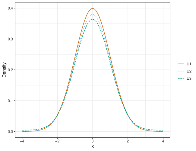
Figure 1: Three density plots of close-to-normal distributions.

All three presented distributions look quite close to the normal one. However, their actual standard deviations are $\sigma_{U1}=1$, $\sigma_{U2}=11$, $\sigma_{U3}=3$. The actual normal distributions with such standard deviations are presented in Figure 2.

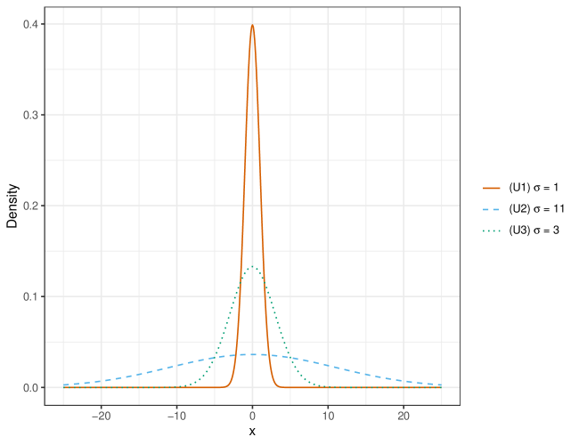
Figure 2: Normal distributions with various standard deviation values.

In fact, only the first distribution is the standard normal distribution $U1=\mathcal{N}(0,1^{2})$. Two other distributions are contaminated normal distributions that are mixtures of two normal distributions (see [Wil16]): $U2=0.95\cdot\mathcal{N}(0,1^{2})+0.05\cdot\mathcal{N}(0,49^{2})$, $U3=0.9\cdot\mathcal{N}(0,1^{2})+0.1\cdot\mathcal{N}(0,9^{2})$. The standard deviation is not a robust measure, its breakdown point is zero. If the data are contaminated, the standard deviation estimations can be misleading because of the high sensitivity to outliers.

In order to solve this problem, we may need a robust measure of the statistical dispersion. A widely used option is the median absolute deviation. One of the first mentions can be found in [Ham74] where it is attributed to Gauss. In [RC93], the median absolute deviation is introduced as a very robust scale estimator because it has the best possible breakdown point (0.5).

Let $X$ be a sample of i.i.d. random variables: $X=\{X_{1},X_{2},\ldots X_{n}\}$. Here is the classic non-scaled definition of the median absolute deviation:

$$\operatorname{MAD}_{0}(X)=\operatorname{median}(|X-\operatorname{median}(X)|).$$

Let us assume that $X$ follows the standard normal distribution: $X\sim\mathcal{N}(0,1^{2})$. If we want to make the median absolute deviation asymptotically consistent with the standard deviation under the normal distribution for an infinitely large sample, we should define a modification of $\operatorname{MAD}_{0}$ with a bias-correction factor $C_{\infty}$:

$$\operatorname{MAD}_{\infty}(X)=C_{\infty}\cdot\operatorname{median}(|X-\operatorname{median}(X)|)=C_{\infty}\cdot\operatorname{MAD}_{0}(X).$$

Since we are building an unbiased estimator, its asymptotic expected value $\lim_{n\to\infty}\mathbb{E}[\operatorname{MAD}_{\infty}(X)]$ should be equal to $1$. It gives us the following equation for $C_{\infty}$:

$$C_{\infty}=\frac{1}{\lim_{n\to\infty}\mathbb{E}[\operatorname{MAD}_{0}(X)]}.$$

Let us denote $\lim_{n\to\infty}\mathbb{E}[\operatorname{MAD}_{0}(|X|)]$ by $M_{\infty}$. Since the median of $\mathcal{N}(0,1^{2})$ is zero, we have:

$$M_{\infty}=\lim_{n\to\infty}\mathbb{E}[\operatorname{median}(|X-\operatorname{median}(X))]=\lim_{n\to\infty}\mathbb{E}[\operatorname{median}(|X|)].$$

Since $M_{\infty}$ is the expected value of the median of $|X|$, we can write

$$\mathbb{P}(|X_{1}|<M_{\infty})=0.5,$$

which is the same as

$$\mathbb{P}(-M_{\infty}<X_{1}<M_{\infty})=0.5.$$

Let us denote the cumulative distribution function of $\mathcal{N}(0,1^{2})$ by $\Phi$. Then, the probability of getting $X_{1}$ from the range $(-M_{\infty};M_{\infty})$ is $\Phi(M_{\infty})-\Phi(-M_{\infty})$. Thus,

$$\Phi(M_{\infty})-\Phi(-M_{\infty})=0.5.$$

Since $\mathcal{N}(0,1^{2})$ is symmetric around zero, $\Phi(-M_{\infty})=1-\Phi(M_{\infty})$. Therefore

$$\Phi(M_{\infty})=0.75.$$

Assuming that $\Phi^{-1}$ is the quantile function of $\mathcal{N}(0,1^{2})$, we have:

$$M_{\infty}=\Phi^{-1}(0.75)\approx 0.674489750196082.$$

Finally,

$$C_{\infty}=\frac{1}{\lim_{n\to\infty}\mathbb{E}[\operatorname{MAD}_{0}(X)]}=\dfrac{1}{M_{\infty}}=\dfrac{1}{\Phi^{-1}(0.75)}\approx 1.4826022185056.$$

Now we consider a scaled median absolute deviation that could be used as an unbiased standard deviation estimator under normality for a finite sample of size $n$. Let us denote it by $\operatorname{MAD}_{n}$:

$$\operatorname{MAD}_{n}(X)=C_{n}\cdot\operatorname{median}(|X-\operatorname{median}(X)|)=C_{n}\cdot\operatorname{MAD}_{0}(X).$$

We cannot use $C_{\infty}$ as a bias-correction factor for finite samples because it would make $\operatorname{MAD}_{n}$ a biased estimator of the standard deviation. To make it unbiased, we have to find proper values of $C_{n}$ for each sample size $n$. These values can be evaluated as

$$C_{n}=\dfrac{1}{\mathbb{E}[\operatorname{MAD}_{0}(X)]}=\dfrac{1}{M_{n}},$$

where $M_{n}=\mathbb{E}[\operatorname{MAD}_{0}(X)]$, $X=\{X_{1},X_{2},\ldots,X_{n}\}$.

2.2 Bias-correction factors based on the sample median

Traditionally, by $\operatorname{median}$ we assume the sample median (if $n$ is odd, the median is the middle order statistic; if $n$ is even, the median is the arithmetic average of the two middle order statistics). This approach is consistent with the Hyndman-Fan Type 7 quantile estimator (see [HF96]) which is the most popular traditional quantile estimator based on one or two order statistics (it is used by default in R, Julia, NumPy, and Excel). To avoid confusion, let us denote the median estimator based on the sample median by $\operatorname{median}_{\operatorname{SM}}$. Similarly, we denote $\operatorname{MAD}$ based on $\operatorname{median}_{\operatorname{SM}}$ by $\operatorname{MAD}_{\operatorname{SM}}$. Let us briefly discuss existing approaches for picking $C_{n}$ values for $\operatorname{median}_{\operatorname{SM}}$.

One of the first attempts to define $C_{n}$ was made in [CR92] by Christophe Croux and Peter J. Rousseeuw. They suggested using the following equations:

$$C_{n}=\dfrac{b_{n}}{\Phi^{-1}(0.75)}.$$

For $n\leq 9$, the approximated values of $b_{n}$ were defined as presented in Table LABEL:tab:croux.

Table 1: Original $b_{n}$ factors from the Croux-Rousseeuw approach.

n	$b_{n}$
2	1.196
3	1.495
4	1.363
5	1.206
6	1.200
7	1.140
8	1.129
9	1.107

For $n>9$, they suggested using the following equation:

$$b_{n}=\dfrac{n}{n-0.8}.$$

This approach was improved in [Wil11] by Dennis C. Williams. Firstly, he provided updated $b_{n}$ values for $n\leq 9$ (see Table LABEL:tab:williams).

Table 2: Williams version of $b_{n}$ factors from the Croux-Rousseeuw approach.

n	$b_{n}$
2	1.197
3	1.490
4	1.360
5	1.217
6	1.189
7	1.138
8	1.127
9	1.101

Secondly, he introduced a small correction for $n>9$:

$$b_{n}=\dfrac{n}{n-0.801}.$$

Thirdly, he discussed another kind of approximation for such kind of bias-correction factors:

$$b_{n}\cong 1+cn^{-d}.$$

In his paper, he applied the above equation only to Shorth (which is the smallest interval that contains at least half of the data points), but this approach can also be applied to other measures of scale.

Next, in [Hay14], Kevin Hayes suggested another kind of prediction equation for $n\geq 9$:

$$C_{n}=\dfrac{1}{\hat{a}_{n}},$$

where

$$\hat{a}_{n}=\Phi^{-1}(0.75)\Bigg{(}1-\dfrac{\alpha}{n}-\dfrac{\beta}{n^{2}}\Bigg{)}.$$

The suggested values of $\alpha$ and $\beta$ are listed in Table LABEL:tab:hayes.

Table 3: $\alpha$ and $\beta$ values from the Hayes approach.

n	$\alpha$	$\beta$
odd	0.7635	0.565
even	0.7612	1.123

Finally, in [PKW20], Chanseok Park, Haewon Kim, and Min Wang aggregated all of the previous results. They used the following form of the main equation:

$$C_{n}=\dfrac{1}{\Phi^{-1}(0.75)\cdot(1+A_{n})}.$$

For $n>100$, they suggested two approaches. The first one is based on [Hay14] (the same equation for both odd and even $n$ values):

$$A_{n}=-\dfrac{0.76213}{n}-\dfrac{0.86413}{n^{2}}.$$

The second one is based on [Wil11]:

$$A_{n}=-0.804168866\cdot n^{-1.008922}.$$

Both approaches produce almost identical results, so it does not actually matter which one to use.

For $2\leq n\leq 100$, they suggested to use predefined constants listed in Table 4 (based on Table A2 from [PKW20]). The corresponding plot is presented in Figure 3.

Table 4: $C_{n}$ factors from the Park approach.

n	$C_{n}$	n	$C_{n}$	n	$C_{n}$	n	$C_{n}$	n	$C_{n}$	n	$C_{n}$	n	$C_{n}$
1	-	21	1.5407	41	1.5111	61	1.5016	81	1.4968	109	1.4931	249	1.4872
2	1.7722	22	1.5393	42	1.5110	62	1.5015	82	1.4968	110	1.4931	250	1.4872
3	2.2049	23	1.5352	43	1.5099	63	1.5010	83	1.4964	119	1.4923	299	1.4864
4	2.0167	24	1.5341	44	1.5095	64	1.5008	84	1.4965	120	1.4922	300	1.4864
5	1.8039	25	1.5305	45	1.5085	65	1.5003	85	1.4963	129	1.4914	349	1.4858
6	1.7638	26	1.5300	46	1.5084	66	1.5003	86	1.4961	130	1.4914	350	1.4858
7	1.6868	27	1.5269	47	1.5075	67	1.4999	87	1.4958	139	1.4908	399	1.4855
8	1.6718	28	1.5264	48	1.5072	68	1.4998	88	1.4958	140	1.4908	400	1.4855
9	1.6329	29	1.5236	49	1.5064	69	1.4993	89	1.4956	149	1.4902	449	1.4852
10	1.6247	30	1.5230	50	1.5063	70	1.4992	90	1.4954	150	1.4902	450	1.4852
11	1.6013	31	1.5207	51	1.5056	71	1.4989	91	1.4953	159	1.4897	499	1.4848
12	1.5962	32	1.5203	52	1.5052	72	1.4988	92	1.4951	160	1.4897	500	1.4848
13	1.5808	33	1.5185	53	1.5046	73	1.4985	93	1.4949	169	1.4893	-	-
14	1.5773	34	1.5179	54	1.5044	74	1.4984	94	1.4950	170	1.4893	-	-
15	1.5663	35	1.5163	55	1.5037	75	1.4979	95	1.4947	179	1.4890	-	-
16	1.5638	36	1.5161	56	1.5036	76	1.4979	96	1.4947	180	1.4889	-	-
17	1.5553	37	1.5144	57	1.5031	77	1.4975	97	1.4944	189	1.4887	-	-
18	1.5534	38	1.5140	58	1.5029	78	1.4975	98	1.4943	190	1.4887	-	-
19	1.5472	39	1.5127	59	1.5023	79	1.4972	99	1.4941	199	1.4883	-	-
20	1.5457	40	1.5124	60	1.5021	80	1.4972	100	1.4942	200	1.4883	-	-

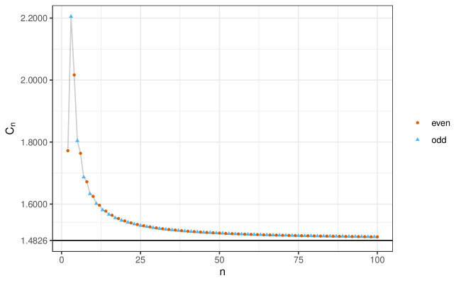
Figure 3: MAD bias-correction factors from the Park approach

2.3 Alternative median estimators

The described approach works quite well in practice for the sample median. This estimator is the most robust median estimator (its breakdown point is 0.5), but it does not have the best possible statistical efficiency since it is based only on one or two order statistics. Fortunately, there are other quantile estimators with better statistical efficiency. One of the most popular alternatives which evaluate the median as a weighted sum of all order statistics is the Harrell-Davis quantile estimator (see [HD82]). Let $Q(X,p)$ be an estimation of the $p^{\textrm{th}}$ quantile of the random sample $X$. The Harrell-Davis quantile estimator $Q_{\operatorname{HD}}(X,p)$ is defined as follows:

$$Q_{\operatorname{HD}}(X,p)=\sum_{i=1}^{n}W_{\operatorname{HD},i}\cdot X_{(i)},\quad W_{\operatorname{HD},i}=I_{i/n}(\alpha,\beta)-I_{(i-1)/n}(\alpha,\beta),$$

where $I_{v}(\alpha,\beta)$ is the regularized incomplete beta function, $\alpha=(n+1)p$, $\;\beta=(n+1)(1-p)$, $X_{(i)}$ is the $i^{\textrm{th}}$ order statistic of $X$.

The Harrell-Davis quantile estimator is suggested in [DN03], [GK12], [Wil16], and [GC20] as an efficient alternative to the sample median. In [YSD85] the Harrell-Davis median estimator is shown to be asymptotically equivalent to the sample median. While $Q_{\operatorname{HD}}$ has great statistical efficiency, it is not robust (its breakdown point is zero). In practice, we still can use $Q_{\operatorname{HD}}$ for medium-size outliers without loss of accuracy because the corresponding $W_{\operatorname{HD},i}$ coefficients are quite small. However, if a sample contains extreme outliers, $Q_{\operatorname{HD}}$ can be corrupted. Other examples of quantile estimators based on a weighted sum of all order statistics are the Sfakianakis-Verginis quantile estimator (see [SV08]) and the Navruz-Özdemir quantile estimator (see [NÖ20]). However, we continue considering only the Harrell-Davis quantile estimator because it is the most popular option in this family.

In order to find an optimal trade-off between robustness and statistical efficiency, we can consider the trimmed Harrell-Davis quantile estimator based on the highest density interval of the given width that we denote by $Q_{\operatorname{THD}}$ (see [Aki22]). In this modification of $Q_{\operatorname{HD}}$, we perform summation only within the highest density interval $[L;R]$ of $\operatorname{Beta}(\alpha,\beta)$ of size $D$ (as a rule of thumb, we can use $D=1/\sqrt{n}$ which gives us an estimator $Q_{\operatorname{THD-SQRT}}$). It can be defined as follows:

$$Q_{\operatorname{THD}}(X,p)=\sum_{i=1}^{n}W_{\operatorname{THD},i}\cdot X_{(i)},\quad W_{\operatorname{THD},i}=F_{\operatorname{THD}}(i/n)-F_{\operatorname{THD}}((i-1)/n),$$

$$F_{\operatorname{THD}}(v)=\begin{cases}0&\textrm{for }\,v<L,\\ \big{(}I_{v}(\alpha,\beta)-I_{L}(\alpha,\beta)\big{)}/\big{(}I_{R}(\alpha,\beta)\big{)}-I_{L}(\alpha,\beta)\big{)}\big{)}&\textrm{for }\,L\leq v\leq R,\\ 1&\textrm{for }\,R<v.\end{cases}$$

Quantile estimators $Q_{\operatorname{HD}}$ and $Q_{\operatorname{THD-SQRT}}$ can be also used as median estimators: $\operatorname{median}_{\operatorname{HD}}(X)=Q_{\operatorname{HD}}(X,0.5)$, $\operatorname{median}_{\operatorname{THD-SQRT}}(X)=Q_{\operatorname{THD-SQRT}}(X,0.5)$. Let us denote the median absolute deviation based on $Q_{\operatorname{HD}}$ by $\operatorname{MAD}_{\operatorname{HD}}$. Similarly, we denote the median absolute deviation based on $Q_{\operatorname{THD-SQRT}}$ by $\operatorname{MAD}_{\operatorname{THD-SQRT}}$.

In this paper, we conduct several simulation studies that evaluate approximated $C_{n}$ values for $\operatorname{MAD}_{\operatorname{SM}}$, $\operatorname{MAD}_{\operatorname{THD}}$, and $\operatorname{MAD}_{\operatorname{THD-SQRT}}$.

3 Simulation study

In this section, we are going to perform several numerical simulations. In Simulation 1, we get empirical values of the bias-correction factors $C_{n}$ for all considered $\operatorname{MAD}$ estimators. In Simulation 2 and Simulation 3, we perform an analysis of statistical efficiency and sensitivity to outliers of the obtained unbiased estimators.

3.1 Simulation 1: Evaluating bias-correction factors using the Monte-Carlo method

Since $C_{n}=1/\mathbb{E}[\operatorname{MAD}_{0}(X)]$, this value can be obtained by estimating the expected value of $\operatorname{MAD}_{0}(X)$ using the Monte-Carlo method. We do it according to the following scheme:

foreach $\textit{median}_{*}\in\{\operatorname{median}_{\operatorname{SM}},\,\operatorname{median}_{\operatorname{HD}},\,\operatorname{median}_{\operatorname{THD-SQRT}}\}$ do

       foreach $n\in\{2..100,\ldots,3000\}$ do

             $\textit{repetitions}\leftarrow\textbf{when}\,\{n\leq 10\to 10^{9};\;n\leq 100\to 5\cdot 10^{8};\;\textbf{else}\to 2\cdot 10^{8}\}$

             for $i\leftarrow 1..\textit{repetitions}$ do

                   $x\leftarrow\textrm{GenerateRandomSample}(\textrm{Distribution}=\mathcal{N}(0,1^{2}),\,\textrm{SampleSize}=n)$

                   $m_{i}\leftarrow\textit{median}_{*}(|x-\textit{median}_{*}(x)|)$

            $M_{n}\leftarrow\sum m_{i}/\textit{repetitions}$

             $C_{n}\leftarrow 1/M_{n}$

      

The estimated $C_{n}$ values for $\operatorname{MAD}_{\operatorname{SM}}$, $\operatorname{MAD}_{\operatorname{HD}}$, $\operatorname{MAD}_{\operatorname{THD-SQRT}}$ are presented in Tables 5, 6, and 7 respectively. A visualization for $2\leq n\leq 100$ is shown in Figure 4. The simulation for $\operatorname{MAD}_{\operatorname{SM}}$ replicates the study from [PKW20] with a higher number of samples (they used $10^{7}$ random samples). The results of two studies (Tables 4 and 5) are quite close to each other (the maximum observed absolute difference is $\approx 0.00065$).

Table 5: $C_{n}$ factors for $\operatorname{MAD}_{\operatorname{SM}}$.

n	$C_{n}$	n	$C_{n}$	n	$C_{n}$	n	$C_{n}$	n	$C_{n}$	n	$C_{n}$	n	$C_{n}$
1	-	21	1.5405	41	1.5117	61	1.5021	81	1.4972	109	1.4933	249	1.4872
2	1.7725	22	1.5393	42	1.5115	62	1.5019	82	1.4971	110	1.4933	250	1.4872
3	2.2049	23	1.5352	43	1.5103	63	1.5014	83	1.4968	119	1.4924	299	1.4864
4	2.0172	24	1.5342	44	1.5101	64	1.5013	84	1.4967	120	1.4924	300	1.4864
5	1.8040	25	1.5307	45	1.5091	65	1.5008	85	1.4965	129	1.4916	349	1.4859
6	1.7637	26	1.5299	46	1.5089	66	1.5007	86	1.4964	130	1.4916	350	1.4859
7	1.6871	27	1.5269	47	1.5080	67	1.5003	87	1.4961	139	1.4910	399	1.4855
8	1.6715	28	1.5263	48	1.5078	68	1.5002	88	1.4961	140	1.4910	400	1.4855
9	1.6326	29	1.5238	49	1.5069	69	1.4998	89	1.4958	149	1.4904	449	1.4852
10	1.6245	30	1.5233	50	1.5067	70	1.4997	90	1.4958	150	1.4904	450	1.4851
11	1.6011	31	1.5212	51	1.5060	71	1.4993	91	1.4955	159	1.4899	499	1.4849
12	1.5961	32	1.5207	52	1.5058	72	1.4992	92	1.4955	160	1.4899	500	1.4849
13	1.5806	33	1.5189	53	1.5051	73	1.4988	93	1.4952	169	1.4895	600	1.4845
14	1.5772	34	1.5184	54	1.5049	74	1.4987	94	1.4952	170	1.4895	700	1.4842
15	1.5661	35	1.5168	55	1.5042	75	1.4984	95	1.4950	179	1.4891	800	1.4840
16	1.5637	36	1.5164	56	1.5041	76	1.4983	96	1.4949	180	1.4891	900	1.4839
17	1.5554	37	1.5149	57	1.5035	77	1.4979	97	1.4947	189	1.4887	1000	1.4837
18	1.5536	38	1.5146	58	1.5033	78	1.4978	98	1.4947	190	1.4887	1500	1.4834
19	1.5471	39	1.5132	59	1.5027	79	1.4975	99	1.4945	199	1.4884	2000	1.4832
20	1.5457	40	1.5129	60	1.5026	80	1.4975	100	1.4944	200	1.4884	3000	1.4830

Table 6: $C_{n}$ factors for $\operatorname{MAD}_{\operatorname{HD}}$.

n	$C_{n}$	n	$C_{n}$	n	$C_{n}$	n	$C_{n}$	n	$C_{n}$	n	$C_{n}$	n	$C_{n}$
1	-	21	1.5252	41	1.5050	61	1.4972	81	1.4933	109	1.4902	249	1.4857
2	1.7725	22	1.5235	42	1.5045	62	1.4969	82	1.4931	110	1.4902	250	1.4857
3	1.5682	23	1.5220	43	1.5039	63	1.4967	83	1.4930	119	1.4896	299	1.4852
4	1.5959	24	1.5204	44	1.5034	64	1.4964	84	1.4928	120	1.4895	300	1.4852
5	1.5661	25	1.5191	45	1.5029	65	1.4962	85	1.4927	129	1.4890	349	1.4848
6	1.5666	26	1.5177	46	1.5025	66	1.4960	86	1.4926	130	1.4889	350	1.4848
7	1.5646	27	1.5164	47	1.5020	67	1.4957	87	1.4924	139	1.4884	399	1.4845
8	1.5591	28	1.5154	48	1.5016	68	1.4955	88	1.4923	140	1.4884	400	1.4845
9	1.5567	29	1.5143	49	1.5011	69	1.4953	89	1.4922	149	1.4880	449	1.4843
10	1.5529	30	1.5133	50	1.5008	70	1.4951	90	1.4921	150	1.4880	450	1.4843
11	1.5496	31	1.5123	51	1.5004	71	1.4950	91	1.4920	159	1.4877	499	1.4841
12	1.5465	32	1.5114	52	1.5000	72	1.4947	92	1.4918	160	1.4876	500	1.4841
13	1.5434	33	1.5106	53	1.4997	73	1.4946	93	1.4917	169	1.4873	600	1.4838
14	1.5406	34	1.5098	54	1.4993	74	1.4944	94	1.4916	170	1.4873	700	1.4836
15	1.5380	35	1.5090	55	1.4990	75	1.4942	95	1.4915	179	1.4871	800	1.4835
16	1.5355	36	1.5083	56	1.4986	76	1.4940	96	1.4914	180	1.4870	900	1.4834
17	1.5332	37	1.5076	57	1.4983	77	1.4939	97	1.4913	189	1.4868	1000	1.4833
18	1.5310	38	1.5069	58	1.4980	78	1.4937	98	1.4912	190	1.4868	1500	1.4831
19	1.5289	39	1.5062	59	1.4977	79	1.4936	99	1.4911	199	1.4866	2000	1.4830
20	1.5270	40	1.5056	60	1.4975	80	1.4934	100	1.4910	200	1.4866	3000	1.4828

Table 7: $C_{n}$ factors for $\operatorname{MAD}_{\operatorname{THD-SQRT}}$.

n	$C_{n}$	n	$C_{n}$	n	$C_{n}$	n	$C_{n}$	n	$C_{n}$	n	$C_{n}$	n	$C_{n}$
1	-	21	1.5417	41	1.5111	61	1.5013	81	1.4965	109	1.4927	249	1.4869
2	1.7725	22	1.5385	42	1.5104	62	1.5010	82	1.4963	110	1.4926	250	1.4869
3	1.6455	23	1.5361	43	1.5097	63	1.5007	83	1.4961	119	1.4919	299	1.4861
4	2.0172	24	1.5333	44	1.5091	64	1.5004	84	1.4959	120	1.4918	300	1.4861
5	1.6774	25	1.5313	45	1.5085	65	1.5001	85	1.4958	129	1.4911	349	1.4856
6	1.6887	26	1.5290	46	1.5078	66	1.4998	86	1.4956	130	1.4910	350	1.4856
7	1.6810	27	1.5272	47	1.5073	67	1.4995	87	1.4955	139	1.4904	399	1.4852
8	1.6363	28	1.5254	48	1.5067	68	1.4993	88	1.4953	140	1.4904	400	1.4852
9	1.6431	29	1.5238	49	1.5063	69	1.4990	89	1.4952	149	1.4899	449	1.4849
10	1.6137	30	1.5224	50	1.5057	70	1.4988	90	1.4950	150	1.4898	450	1.4849
11	1.6036	31	1.5210	51	1.5053	71	1.4986	91	1.4949	159	1.4894	499	1.4847
12	1.5938	32	1.5198	52	1.5048	72	1.4983	92	1.4947	160	1.4894	500	1.4847
13	1.5826	33	1.5185	53	1.5044	73	1.4981	93	1.4946	169	1.4890	600	1.4843
14	1.5771	34	1.5175	54	1.5039	74	1.4979	94	1.4944	170	1.4890	700	1.4841
15	1.5683	35	1.5163	55	1.5035	75	1.4977	95	1.4943	179	1.4886	800	1.4839
16	1.5639	36	1.5155	56	1.5031	76	1.4974	96	1.4942	180	1.4886	900	1.4837
17	1.5574	37	1.5144	57	1.5027	77	1.4972	97	1.4940	189	1.4883	1000	1.4836
18	1.5530	38	1.5136	58	1.5024	78	1.4970	98	1.4940	190	1.4883	1500	1.4833
19	1.5488	39	1.5127	59	1.5020	79	1.4969	99	1.4938	199	1.4880	2000	1.4831
20	1.5449	40	1.5119	60	1.5017	80	1.4966	100	1.4937	200	1.4880	3000	1.4829

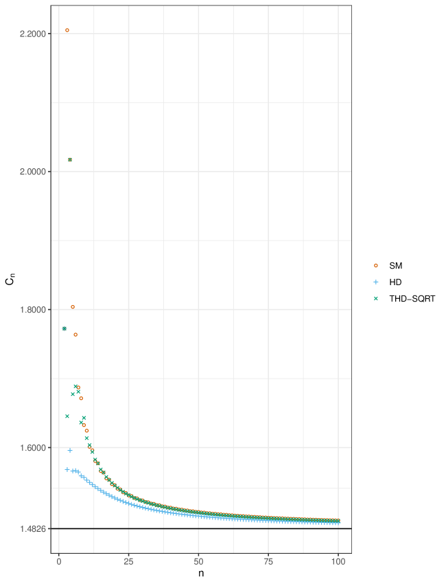
Figure 4: Bias-correction factors using different median estimators.

3.2 Simulation 2: Statistical efficiency of the median absolute deviation

In this simulation, we estimate the relative efficiency $e$ of $\operatorname{MAD}_{\operatorname{HD}}$ and $\operatorname{MAD}_{\operatorname{THD-SQRT}}$ against $\operatorname{MAD}_{\operatorname{SM}}$ (the baseline). It can be calculated as the ratio of the estimator mean squared errors ($\operatorname{MSE}$) (see [Dek+05]). Since all the estimators are unbiased under normality, $\operatorname{MSE}(\operatorname{MAD}_{*})=\mathbb{V}[\operatorname{MAD}_{*}]$. Thus, we have:

$$e(\operatorname{MAD}_{*})=\dfrac{\operatorname{MSE}(\operatorname{MAD}_{\operatorname{SM}})}{\operatorname{MSE}(\operatorname{MAD}_{*})}=\dfrac{\mathbb{V}[\operatorname{MAD}_{\operatorname{SM}}(X)]}{\mathbb{V}[\operatorname{MAD}_{*}(X)]},$$

where $\mathbb{V}$ is the variance of $\operatorname{MAD}_{n}$ for the given sample size $n$, $\operatorname{MAD}_{*}$ is a placeholder for $\operatorname{MAD}_{\operatorname{HD}}$ and $\operatorname{MAD}_{\operatorname{THD-SQRT}}$. We conduct this simulation according to the following scheme:

foreach $n\in\{2,3,4,5,6,7,10,50,100,500,1000\}$ do

       for $i\leftarrow 1..10\,000$ do

             $x\leftarrow\textrm{GenerateRandomSample}(\textrm{Distribution}=\mathcal{N}(0,1^{2}),\,\textrm{SampleSize}=n)$

             $m_{\operatorname{SM},i}=\operatorname{MAD}_{\operatorname{SM},n}(x)$

             $m_{\operatorname{HD},i}=\operatorname{MAD}_{\operatorname{HD},n}(x)$

             $m_{\operatorname{THD-SQRT},i}=\operatorname{MAD}_{\operatorname{THD-SQRT},n}(x)$

            

      $e(\operatorname{MAD}_{\operatorname{HD},n})=\mathbb{V}(m_{\operatorname{SM},\{i\}})/\mathbb{V}(m_{\operatorname{HD},\{i\}})$

       $e(\operatorname{MAD}_{\operatorname{THD-SQRT},n})=\mathbb{V}(m_{\operatorname{SM},\{i\}})/\mathbb{V}(m_{\operatorname{THD-SQRT},\{i\}})$

      

The evaluated values of the $e(\operatorname{MAD}_{\operatorname{HD}})$ and $e(\operatorname{MAD}_{\operatorname{THD-SQRT}})$ are presented in Table 8.

Table 8: Relative statistical efficiency of the median absolute deviation.

n	HD	THD-SQRT
2	1.000	1.000
3	2.473	2.331
4	1.618	1.000
5	1.854	1.468
6	1.473	1.180
7	1.688	1.326
8	1.379	1.141
9	1.527	1.227
10	1.342	1.129
50	1.156	1.075
100	1.110	1.054
500	1.047	1.025
1000	1.035	1.018

Based on the obtained measurements, we can do the following observations about the efficiency of the considered $\operatorname{MAD}$ estimators under the normal distribution:

• Both $\operatorname{MAD}_{\operatorname{HD}}$ and $\operatorname{MAD}_{\operatorname{THD-SQRT}}$ are more efficient than $\operatorname{MAD}_{\operatorname{SM}}$.

• $\operatorname{MAD}_{\operatorname{HD}}$ is more efficient than $\operatorname{MAD}_{\operatorname{THD-SQRT}}$.

• The impact of using $\operatorname{MAD}_{\operatorname{HD}}$ and $\operatorname{MAD}_{\operatorname{THD-SQRT}}$ instead of $\operatorname{MAD}_{\operatorname{SM}}$ is most noticeable for small samples (except $n=2$ for $\operatorname{MAD}_{\operatorname{HD}}$ and $n\in\{2,4\}$ for $\operatorname{MAD}_{\operatorname{THD-SQRT}}$). The most impressive boost of efficiency can be observed for $n=3$: $+147.3\%$ for $\operatorname{MAD}_{\operatorname{HD}}$ and $+133.1\%$ for $\operatorname{MAD}_{\operatorname{THD-SQRT}}$.

• For large samples, $\operatorname{MAD}_{\operatorname{HD}}$ and $\operatorname{MAD}_{\operatorname{THD-SQRT}}$ are still more efficient than $\operatorname{MAD}_{\operatorname{SM}}$, but the difference is not so noticeable. For example, for $n=1000$, $\operatorname{MAD}_{\operatorname{HD}}$ gives $+3.5\%$ and $\operatorname{MAD}_{\operatorname{THD-SQRT}}$ gives $+1.8\%$ to statistical efficiency.

3.3 Simulation 3: Sensitivity to outliers of the median absolute deviation

There are various metrics that describe robustness (e.g., the breakdown point, the influence function, and the sensitivity curve). While these metrics provide important theoretical properties, they do not present a clear visual illustration of the actual impact of outliers on estimations. Another approach to getting an idea of the sensitivity of different estimators to outliers is exploring the statistical dispersion of obtained estimations on light-tailed and heavy-tailed distributions. Let us conduct a simulation according to the following scheme:

foreach $d\in\mathcal{D}$ do

       foreach $n\in\{2,3,4,5,6,7,8,9,10,50,100,500,1000\}$ do

             for $i\leftarrow 1..1\,000$ do

                   $x\leftarrow\textrm{GenerateRandomSample}(\textrm{Distribution}=d,\,\textrm{SampleSize}=n)$

                   foreach $\textit{estimator}\in\{\operatorname{SM},\operatorname{HD},\operatorname{THD-SQRT}\}$ do

                         $m_{\textit{estimator},i}=\operatorname{MAD}_{\textit{estimator},n}(x)$

                        

                  

            foreach $\textit{aggregator}\in\{\operatorname{SD},\operatorname{IQR},\operatorname{MAD}_{\operatorname{SM}}\}$ do

                   $\operatorname{Result}(d,n,\textit{estimator},\textit{aggregator})=\textit{aggregator}(m_{\textit{estimator},\{i\}})$

            

      

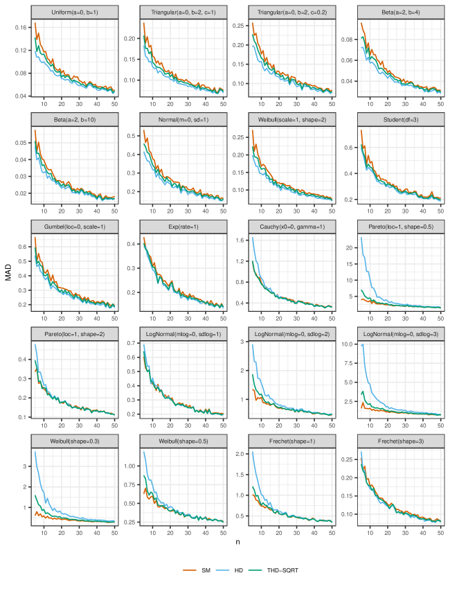
Figure 5: Statistical dispersion of MAD estimations on various distributions.

In this simulation, we enumerate a set $\mathcal{D}$ of distributions listed in Table LABEL:tab:ds (this set includes symmetric and skewed, light-tailed and heavy-tailed distributions). We describe the statistical dispersion of each set of $\operatorname{MAD}_{n}$ estimations in three different ways: $\operatorname{SD}$ (the classic standard deviation), $\operatorname{IQR}$ (interquartile range based on Hyndman-Fan Type 7 quantile estimator), $\operatorname{MAD}_{\operatorname{SM}}$. The aggregated results for $n\in\{5,6,10,50\}$ are listed in Tables 10, 11,12, 13 respectively. The $\operatorname{MAD}_{\operatorname{SM}}$-aggregated results for all values of $n$ are presented in Figure 5. Based on the obtained measurements, we can make the following observations:

• For the light-tailed distributions, $\operatorname{MAD}_{\operatorname{HD}}$ has the best robustness, $\operatorname{MAD}_{\operatorname{SM}}$ has the worst robustness.

• For the heavy-tailed distributions, the opposite is true: $\operatorname{MAD}_{\operatorname{HD}}$ has the worst robustness, $\operatorname{MAD}_{\operatorname{SM}}$ has the best robustness. On small samples, $\operatorname{MAD}_{\operatorname{HD}}$ could be much worse than $\operatorname{MAD}_{\operatorname{SM}}$ while $\operatorname{MAD}_{\operatorname{THD-SQRT}}$ is just a little bit worse.

• For $n\geq 50$, the difference between all considered estimators is negligible.

Table 9: Distributions for Simulation 3.

Distribution	Support	Skewness	Tailness
Uniform(a=0, b=1)	$[0;1]$	Symmetric	Light-tailed
Triangular(a=0, b=2, c=1)	$[0;2]$	Symmetric	Light-tailed
Triangular(a=0, b=2, c=0.2)	$[0;2]$	Right-skewed	Light-tailed
Beta(a=2, b=4)	$[0;1]$	Right-skewed	Light-tailed
Beta(a=2, b=10)	$[0;1]$	Right-skewed	Light-tailed
Normal(m=0, sd=1)	$(-\infty;+\infty)$	Symmetric	Light-tailed
Weibull(scale=1, shape=2)	$[0;+\infty)$	Right-skewed	Light-tailed
Student(df=3)	$(-\infty;+\infty)$	Symmetric	Light-tailed
Gumbel(loc=0, scale=1)	$(-\infty;+\infty)$	Right-skewed	Light-tailed
Exp(rate=1)	$[0;+\infty)$	Right-skewed	Light-tailed
Cauchy(x0=0, gamma=1)	$(-\infty;+\infty)$	Symmetric	Heavy-tailed
Pareto(loc=1, shape=0.5)	$[1;+\infty)$	Right-skewed	Heavy-tailed
Pareto(loc=1, shape=2)	$[1;+\infty)$	Right-skewed	Heavy-tailed
LogNormal(mlog=0, sdlog=1)	$(0;+\infty)$	Right-skewed	Heavy-tailed
LogNormal(mlog=0, sdlog=2)	$(0;+\infty)$	Right-skewed	Heavy-tailed
LogNormal(mlog=0, sdlog=3)	$(0;+\infty)$	Right-skewed	Heavy-tailed
Weibull(shape=0.3)	$[0;+\infty)$	Right-skewed	Heavy-tailed
Weibull(shape=0.5)	$[0;+\infty)$	Right-skewed	Heavy-tailed
Frechet(shape=1)	$(0;+\infty)$	Right-skewed	Heavy-tailed
Frechet(shape=3)	$(0;+\infty)$	Right-skewed	Heavy-tailed

Table 10: Properties of MAD estimations for n=5.

	SD			IQR			MAD
Distribution	SM	HD	THD	SM	HD	THD	SM	HD	THD
Uniform(a=0, b=1)	0.16	0.12	0.14	0.23	0.16	0.19	0.17	0.12	0.14
Triangular(a=0, b=2, c=1)	0.24	0.17	0.19	0.33	0.25	0.28	0.24	0.18	0.21
Triangular(a=0, b=2, c=0.2)	0.25	0.20	0.22	0.36	0.27	0.31	0.26	0.20	0.23
Beta(a=2, b=4)	0.10	0.07	0.08	0.13	0.10	0.11	0.10	0.07	0.08
Beta(a=2, b=10)	0.06	0.05	0.05	0.08	0.07	0.07	0.06	0.05	0.05
Normal(m=0, sd=1)	0.59	0.43	0.48	0.72	0.57	0.65	0.53	0.42	0.46
Weibull(scale=1, shape=2)	0.26	0.20	0.22	0.38	0.27	0.30	0.27	0.20	0.22
Student(df=3)	0.79	0.75	0.74	1.00	0.83	0.86	0.74	0.60	0.62
Gumbel(loc=0, scale=1)	0.77	0.58	0.63	0.93	0.76	0.83	0.67	0.54	0.60
Exp(rate=1)	0.51	0.44	0.46	0.63	0.54	0.56	0.43	0.39	0.40
Cauchy(x0=0, gamma=1)	1.90	10.92	2.41	1.70	3.03	1.84	1.18	1.66	1.21
Pareto(loc=1, shape=0.5)	26.80	1645746.00	154.80	7.68	68.61	15.27	3.94	23.28	7.01
Pareto(loc=1, shape=2)	0.56	1.03	0.63	0.53	0.69	0.57	0.34	0.48	0.39
LogNormal(mlog=0, sdlog=1)	0.85	0.99	0.91	0.86	1.00	0.91	0.60	0.69	0.64
LogNormal(mlog=0, sdlog=2)	3.32	18.33	4.39	2.17	5.57	3.04	1.34	2.91	1.87
LogNormal(mlog=0, sdlog=3)	14.53	833.22	31.64	3.83	24.28	7.20	1.59	9.76	3.39
Weibull(shape=0.3)	3.81	16.26	7.23	1.42	7.50	3.36	0.60	3.72	1.59
Weibull(shape=0.5)	1.45	2.08	1.73	1.14	1.87	1.38	0.63	1.19	0.87
Frechet(shape=1)	4.52	52.16	9.99	1.65	3.62	1.87	1.01	2.06	1.21
Frechet(shape=3)	0.33	0.37	0.33	0.36	0.38	0.34	0.25	0.27	0.24

Table 11: Properties of MAD estimations for n=6.

	SD			IQR			MAD
Distribution	SM	HD	THD	SM	HD	THD	SM	HD	THD
Uniform(a=0, b=1)	0.14	0.11	0.12	0.19	0.14	0.16	0.14	0.11	0.12
Triangular(a=0, b=2, c=1)	0.19	0.16	0.18	0.25	0.21	0.24	0.19	0.16	0.18
Triangular(a=0, b=2, c=0.2)	0.22	0.18	0.20	0.30	0.27	0.29	0.22	0.19	0.21
Beta(a=2, b=4)	0.09	0.07	0.08	0.12	0.10	0.11	0.09	0.07	0.08
Beta(a=2, b=10)	0.05	0.04	0.04	0.06	0.05	0.06	0.04	0.04	0.04
Normal(m=0, sd=1)	0.46	0.38	0.42	0.64	0.53	0.59	0.46	0.39	0.44
Weibull(scale=1, shape=2)	0.22	0.18	0.20	0.29	0.25	0.27	0.21	0.18	0.20
Student(df=3)	0.69	0.63	0.65	0.81	0.76	0.76	0.59	0.55	0.56
Gumbel(loc=0, scale=1)	0.54	0.48	0.51	0.69	0.63	0.66	0.50	0.46	0.48
Exp(rate=1)	0.44	0.43	0.42	0.54	0.54	0.54	0.39	0.39	0.38
Cauchy(x0=0, gamma=1)	1.73	15.51	1.94	1.41	2.21	1.47	1.00	1.40	1.02
Pareto(loc=1, shape=0.5)	51.23	12909.42	72.10	7.91	55.16	13.44	4.18	17.87	6.23
Pareto(loc=1, shape=2)	0.46	0.67	0.49	0.51	0.63	0.53	0.35	0.43	0.36
LogNormal(mlog=0, sdlog=1)	0.76	0.87	0.77	0.75	0.88	0.81	0.52	0.61	0.54
LogNormal(mlog=0, sdlog=2)	2.65	11.50	3.09	1.97	4.05	2.55	1.30	2.32	1.52
LogNormal(mlog=0, sdlog=3)	14.29	192.92	24.39	4.74	20.40	7.43	2.35	9.98	3.83
Weibull(shape=0.3)	4.17	11.45	5.16	1.67	5.81	2.89	0.80	3.00	1.36
Weibull(shape=0.5)	1.23	1.72	1.34	1.14	1.72	1.31	0.70	1.08	0.83
Frechet(shape=1)	2.03	10.32	2.30	1.50	3.10	1.79	0.99	1.74	1.13
Frechet(shape=3)	0.28	0.30	0.28	0.31	0.31	0.30	0.22	0.22	0.22

Table 12: Properties of MAD estimations for n=10.

	SD			IQR			MAD
Distribution	SM	HD	THD	SM	HD	THD	SM	HD	THD
Uniform(a=0, b=1)	0.11	0.09	0.11	0.16	0.14	0.15	0.12	0.10	0.11
Triangular(a=0, b=2, c=1)	0.16	0.14	0.15	0.21	0.18	0.19	0.16	0.13	0.14
Triangular(a=0, b=2, c=0.2)	0.17	0.15	0.16	0.24	0.21	0.22	0.18	0.16	0.17
Beta(a=2, b=4)	0.06	0.06	0.06	0.09	0.08	0.08	0.07	0.06	0.06
Beta(a=2, b=10)	0.04	0.03	0.04	0.05	0.04	0.05	0.04	0.03	0.04
Normal(m=0, sd=1)	0.37	0.32	0.35	0.51	0.43	0.47	0.38	0.32	0.34
Weibull(scale=1, shape=2)	0.17	0.15	0.16	0.23	0.20	0.21	0.17	0.15	0.16
Student(df=3)	0.52	0.47	0.49	0.66	0.60	0.62	0.48	0.43	0.45
Gumbel(loc=0, scale=1)	0.42	0.38	0.41	0.58	0.53	0.55	0.43	0.39	0.40
Exp(rate=1)	0.32	0.31	0.31	0.43	0.40	0.41	0.31	0.29	0.30
Cauchy(x0=0, gamma=1)	0.99	1.46	1.01	1.12	1.24	1.08	0.79	0.88	0.76
Pareto(loc=1, shape=0.5)	17.81	275359.25	36.33	5.99	21.77	7.51	3.67	10.20	4.53
Pareto(loc=1, shape=2)	0.29	0.32	0.29	0.34	0.37	0.35	0.25	0.27	0.25
LogNormal(mlog=0, sdlog=1)	0.49	0.51	0.49	0.57	0.62	0.58	0.41	0.45	0.43
LogNormal(mlog=0, sdlog=2)	1.75	2.68	1.98	1.65	2.28	1.78	1.07	1.56	1.18
LogNormal(mlog=0, sdlog=3)	5.23	18.53	6.12	2.77	7.80	3.69	1.60	4.72	2.21
Weibull(shape=0.3)	1.97	3.57	2.44	1.09	2.84	1.59	0.59	1.73	0.90
Weibull(shape=0.5)	0.83	0.93	0.84	0.89	1.08	0.94	0.60	0.74	0.63
Frechet(shape=1)	1.07	2.21	1.19	1.04	1.47	1.13	0.74	1.02	0.76
Frechet(shape=3)	0.19	0.19	0.19	0.25	0.24	0.24	0.18	0.17	0.18

Table 13: Properties of MAD estimations for n=50.

	SD			IQR			MAD
Distribution	SM	HD	THD	SM	HD	THD	SM	HD	THD
Uniform(a=0, b=1)	0.05	0.05	0.05	0.07	0.07	0.07	0.05	0.05	0.05
Triangular(a=0, b=2, c=1)	0.07	0.07	0.07	0.11	0.09	0.10	0.08	0.07	0.07
Triangular(a=0, b=2, c=0.2)	0.08	0.08	0.08	0.11	0.10	0.11	0.08	0.08	0.08
Beta(a=2, b=4)	0.03	0.03	0.03	0.04	0.04	0.04	0.03	0.03	0.03
Beta(a=2, b=10)	0.02	0.02	0.02	0.02	0.02	0.02	0.02	0.02	0.02
Normal(m=0, sd=1)	0.17	0.16	0.16	0.22	0.21	0.22	0.16	0.16	0.16
Weibull(scale=1, shape=2)	0.07	0.07	0.07	0.10	0.09	0.09	0.07	0.07	0.07
Student(df=3)	0.21	0.20	0.20	0.28	0.26	0.26	0.21	0.19	0.20
Gumbel(loc=0, scale=1)	0.20	0.19	0.19	0.26	0.24	0.25	0.19	0.18	0.19
Exp(rate=1)	0.15	0.14	0.14	0.19	0.18	0.19	0.14	0.14	0.14
Cauchy(x0=0, gamma=1)	0.36	0.34	0.35	0.46	0.44	0.44	0.33	0.33	0.32
Pareto(loc=1, shape=0.5)	1.83	2.02	1.87	2.05	2.25	2.04	1.42	1.55	1.48
Pareto(loc=1, shape=2)	0.12	0.12	0.12	0.16	0.15	0.15	0.11	0.11	0.11
LogNormal(mlog=0, sdlog=1)	0.20	0.19	0.20	0.28	0.27	0.27	0.20	0.20	0.20
LogNormal(mlog=0, sdlog=2)	0.53	0.54	0.52	0.66	0.65	0.64	0.47	0.48	0.48
LogNormal(mlog=0, sdlog=3)	0.97	1.05	0.96	1.01	1.20	1.05	0.71	0.82	0.74
Weibull(shape=0.3)	0.38	0.42	0.38	0.40	0.46	0.42	0.28	0.33	0.29
Weibull(shape=0.5)	0.29	0.28	0.28	0.35	0.35	0.34	0.26	0.25	0.25
Frechet(shape=1)	0.40	0.41	0.40	0.50	0.48	0.47	0.36	0.34	0.34
Frechet(shape=3)	0.08	0.08	0.08	0.11	0.11	0.11	0.08	0.08	0.08

4 Special cases of bias-correction factors

In this section, we consider two following cases:

• $n=2$: it is the only case when we can easily calculate the exact value of the bias correction factor.

• $n>100$: for this case, we draw a generic equation following the approach from [Hay14].

4.1 Bias-correction factors for n = 2

Let $X=\{X_{1},X_{2}\}$ be a sample of two i.i.d. random variables from the standard normal distribution $\mathcal{N}(0,1^{2})$. Regardless of the chosen median estimator, the median is unequivocally determined:

$$\operatorname{median}(X)=\dfrac{X_{1}+X_{2}}{2}.$$

Now we calculate the median absolute deviation $\operatorname{MAD}_{0}$:

$$\begin{split}\operatorname{MAD}_{0}(X)&=\operatorname{median}(|X-\operatorname{median}(X)|)=\\ &=\operatorname{median}(\{\,|X_{1}-(X_{1}+X_{2})/2|\,,\,|X_{2}-(X_{1}+X_{2})/2|\,\})=\\ &=\operatorname{median}(\{\,|(X_{1}-X_{2})/2|\,,\,|(X_{2}-X_{1})/2|\,\})=\\ &=|X_{1}-X_{2}|/2.\end{split}$$

Since $X_{1},X_{2}\sim\mathcal{N}(0,1^{2})$ which is symmetric, $|X_{1}-X_{2}|/2$ is distributed the same way as $|X_{1}+X_{2}|/2$. Let us denote the sum of two standard normal distributions by $Z=X_{1}+X_{2}$. It gives us another normal distribution with modified variance:

$$Z\sim\mathcal{N}(0,\sqrt{2}^{2}).$$

Since we take the absolute value of $Z$, we get the half-normal distribution. The expected value of a half-normal distribution which is formed from the normal distribution $\mathcal{N}(0,\sigma^{2})$ is $\sigma\sqrt{2/\pi}$. Thus,

$$\mathbb{E}[|Z|]=\sqrt{2}\sqrt{2/\pi}=2/\sqrt{\pi}.$$

Finally, we have:

$$\mathbb{E}[\operatorname{MAD}_{0}(X)]=\mathbb{E}\Bigg{[}\frac{|X_{1}-X_{2}|}{2}\Bigg{]}=\mathbb{E}\Bigg{[}\frac{|X_{1}+X_{2}|}{2}\Bigg{]}=\mathbb{E}\Bigg{[}\frac{|Z|}{2}\Bigg{]}=\frac{2/\sqrt{\pi}}{2}=\frac{1}{\sqrt{\pi}}.$$

The bias-correction factor $C_{2}$ is the reciprocal value of the expected value of $\operatorname{MAD}_{0}(X)$:

$$C_{2}=\frac{1}{\mathbb{E}[\operatorname{MAD}_{0}(X)]}=\sqrt{\pi}\approx 1.77245385090552.$$

4.2 Bias-correction factors for n > 100

Following the approach from [Hay14], we are going to draw a generic equation for $C_{n}$ in the following form:

$$C_{n}=\dfrac{1}{\Phi^{-1}(0.75)\cdot(1+A_{n})},\quad A_{n}=\dfrac{\alpha}{n}+\dfrac{\beta}{n^{2}}.$$

The coefficients $\alpha$ and $\beta$ can be obtained using least squares on the values from Tables 4 (let us denote $\operatorname{MAD}$ based on this table by $\operatorname{MAD}_{\operatorname{PARK}}$), 5, 6, and 7 for $100<n\leq 500$. The results are presented in Table 14.

Table 14: $A_{n}$ parameters for $n>100$.

	$\alpha$	$\beta$
$\operatorname{MAD}_{\operatorname{PARK}}$	-0.7591	-1.3239
$\operatorname{MAD}_{\operatorname{SM}}$	-0.7668	-2.1897
$\operatorname{MAD}_{\operatorname{HD}}$	-0.4912	-7.6350
$\operatorname{MAD}_{\operatorname{THD-SQRT}}$	-0.6954	-4.9261

The value of $\alpha$ for $\operatorname{MAD}_{\operatorname{PARK}}$ and $\operatorname{MAD}_{\operatorname{SM}}$ are quite close to the suggested $\alpha=-0.76213$ from [PKW20]. The corresponding value of $\beta$ is not so close to $\beta=-0.86413$ from [PKW20], but this difference does not produce a noticeable impact on the final result.

The evaluated values of $\alpha$ and $\beta$ for all $\operatorname{MAD}$ estimators look quite accurate. In Figure 6, we can see the actual (points) and predicted (line) values of $C_{n}$ for $100<n\leq 3000$. Within values $500<n\leq 3000$ from Tables 5, 6, and 7 (that were not used to get the values of $\alpha$ and $\beta$), the maximum observed absolute difference between the actual and predicted values is $\approx 0.000061$.

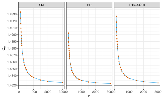
Figure 6: Actual and predicted bias-correction factors

5 Summary

The median absolute deviation is a robust measure of statistical dispersion that can be used as a consistent estimator for the standard deviation under the normal distribution. To make it unbiased, we have to use a bias-correction factor $C_{n}$:

$$\operatorname{MAD}_{n}(X)=C_{n}\cdot\operatorname{median}(|X-\operatorname{median}(X)|).$$

This approach heavily depends on the chosen median estimator. In this paper, we have discussed three estimators: the classic sample median ($\operatorname{median}_{\operatorname{SM}}$), the Harrell-Davis quantile estimator ($\operatorname{median}_{\operatorname{HD}}$), and the trimmed Harrell-Davis quantile estimator based on the highest density interval of the width $1/\sqrt{n}$ ($\operatorname{median}_{\operatorname{THD-SQRT}}$) which give us estimators $\operatorname{MAD}_{\operatorname{SM}}$ and $\operatorname{MAD}_{\operatorname{HD}}$, and $\operatorname{MAD}_{\operatorname{THD-SQRT}}$ respectively.

In Simulation 1, we estimated values of $C_{n}$ using the Monte-Carlo simulation for each estimator. These values are listed in Tables 5, 6, and 7. These tables cover all values of $n$ from $2$ to $100$ and some greater values up to $3000$. A generic approach for large sample sizes ($n>100$) can be presented in the following form:

$$C_{n}=\dfrac{1}{\Phi^{-1}(0.75)\cdot(1+\alpha/n+\beta/n^{2})},$$

where the values of $\alpha$ and $\beta$ are listed in Table 14. For $n=2$, we know the exact value of the bias-correction factor: $C_{2}=\sqrt{\pi}\approx 1.77245385090552$.

In Simulation 2, we evaluated the relative statistical efficiency of $\operatorname{MAD}_{\operatorname{HD}}$ and $\operatorname{MAD}_{\operatorname{THD-SQRT}}$ against $\operatorname{MAD}_{\operatorname{SM}}$. It turned out that the efficiency of $\operatorname{MAD}_{\operatorname{HD}}$ and $\operatorname{MAD}_{\operatorname{THD-SQRT}}$ are noticeably higher than the efficiency of $\operatorname{MAD}_{\operatorname{SM}}$.

In Simulation 3, we investigated the sensitivity to outliers of all $\operatorname{MAD}$ estimators. It turned out that $\operatorname{MAD}_{\operatorname{HD}}$ could be corrupted by extreme outliers in the case of heavy-tailed distributions. Meanwhile, $\operatorname{MAD}_{\operatorname{THD-SQRT}}$ is much more resistant to outliers (while it is still not as robust as $\operatorname{MAD}_{\operatorname{SM}}$).

Thus, in the case of light-tailed distributions, we recommend $\operatorname{MAD}_{\operatorname{HD}}$ as an alternative to the classic $\operatorname{MAD}_{\operatorname{SM}}$ because it has higher statistical efficiency. In the case of heavy-tailed distributions, we recommend $\operatorname{MAD}_{\operatorname{THD-SQRT}}$ because it allows achieving a good trade-off between statistical efficiency and robustness. The practical impact of both approaches is most noticeable for samples with a small number of elements.

The trade-off between the statistical efficiency and the robustness can be customized by choosing another width of the Beta distribution’s highest density interval in $\operatorname{MAD}_{\operatorname{THD}}$. The exact value of this width should be carefully chosen based on the knowledge of the considered distribution, the expected number and the magnitude of possible outliers, and the robustness requirements. The values of the bias-correction factors $C_{n}$ should be properly updated using another Monte-Carlo simulation study similar to Simulation 1.

Disclosure statement

The author reports there are no competing interests to declare.

Data and source code availability

The source code of this paper, the source code of all simulations, and the simulation results are available on GitHub: https://github.com/AndreyAkinshin/paper-mad-factors.

A  Reference implementation

Here is an R implementation of the suggested $\operatorname{MAD}$ estimators:

quantile.hd <- function(x, probs) sapply(probs, function(p) {

  n <- length(x)

  if (n == 0) return(NA)

  if (n == 1) return(x)

  x <- sort(x)

  a <- (n + 1) * p; b <- (n + 1) * (1 - p)

  cdfs <- pbeta(0:n/n, a, b)

  W <- tail(cdfs, -1) - head(cdfs, -1)

  sum(x * W)

})

quantile.thd <- function(x, probs, width = 1/sqrt(length(x))) sapply(probs, function(p) {

  getBetaHdi <- function(a, b, width) {

    eps <- 1e-9

    if (a < 1 + eps & b < 1 + eps) # Degenerate case

      return(c(NA, NA))

    if (a < 1 + eps & b > 1) # Left border case

      return(c(0, width))

    if (a > 1 & b < 1 + eps) # Right border case

      return(c(1 - width, 1))

    if (width > 1 - eps)

      return(c(0, 1))

    # Middle case

    mode <- (a - 1) / (a + b - 2)

    pdf <- function(x) dbeta(x, a, b)

    l <- uniroot(

      f = function(x) pdf(x) - pdf(x + width),

      lower = max(0, mode - width),

      upper = min(mode, 1 - width),

      tol = 1e-9

    )$root

    r <- l + width

    return(c(l, r))

  }

  n <- length(x)

  if (n == 0) return(NA)

  if (n == 1) return(x)

  x <- sort(x)

  a <- (n + 1) * p; b <- (n + 1) * (1 - p)

  hdi <- getBetaHdi(a, b, width)

  hdiCdf <- pbeta(hdi, a, b)

  cdf <- function(xs) {

    xs[xs <= hdi[1]] <- hdi[1]

    xs[xs >= hdi[2]] <- hdi[2]

    (pbeta(xs, a, b) - hdiCdf[1]) / (hdiCdf[2] - hdiCdf[1])

  }

  iL <- floor(hdi[1] * n); iR <- ceiling(hdi[2] * n)

  cdfs <- cdf(iL:iR/n)

  W <- tail(cdfs, -1) - head(cdfs, -1)

  sum(x[(iL + 1):iR] * W)

})

med.sm <- function(x) median(x)

med.hd <- function(x) quantile.hd(x, 0.5)

med.thd.sqrt <- function(x) quantile.thd(x, 0.5)

factors.sm <- c(

      NA, 1.7725, 2.2049, 2.0172, 1.8040, 1.7637, 1.6871, 1.6715, 1.6326, 1.6245,

  1.6011, 1.5961, 1.5806, 1.5772, 1.5661, 1.5637, 1.5554, 1.5536, 1.5471, 1.5457,

  1.5405, 1.5393, 1.5352, 1.5342, 1.5307, 1.5299, 1.5269, 1.5263, 1.5238, 1.5233,

  1.5212, 1.5207, 1.5189, 1.5184, 1.5168, 1.5164, 1.5149, 1.5146, 1.5132, 1.5129,

  1.5117, 1.5115, 1.5103, 1.5101, 1.5091, 1.5089, 1.5080, 1.5078, 1.5069, 1.5067,

  1.5060, 1.5058, 1.5051, 1.5049, 1.5042, 1.5041, 1.5035, 1.5033, 1.5027, 1.5026,

  1.5021, 1.5019, 1.5014, 1.5013, 1.5008, 1.5007, 1.5003, 1.5002, 1.4998, 1.4997,

  1.4993, 1.4992, 1.4988, 1.4987, 1.4984, 1.4983, 1.4979, 1.4978, 1.4975, 1.4975,

  1.4972, 1.4971, 1.4968, 1.4967, 1.4965, 1.4964, 1.4961, 1.4961, 1.4958, 1.4958,

  1.4955, 1.4955, 1.4952, 1.4952, 1.4950, 1.4949, 1.4947, 1.4947, 1.4945, 1.4944)

factors.hd <- c(

      NA, 1.7725, 1.5682, 1.5959, 1.5661, 1.5666, 1.5646, 1.5591, 1.5567, 1.5529,

  1.5496, 1.5465, 1.5434, 1.5406, 1.5380, 1.5355, 1.5332, 1.5310, 1.5289, 1.5270,

  1.5252, 1.5235, 1.5220, 1.5204, 1.5191, 1.5177, 1.5164, 1.5154, 1.5143, 1.5133,

  1.5123, 1.5114, 1.5106, 1.5098, 1.5090, 1.5083, 1.5076, 1.5069, 1.5062, 1.5056,

  1.5050, 1.5045, 1.5039, 1.5034, 1.5029, 1.5025, 1.5020, 1.5016, 1.5011, 1.5008,

  1.5004, 1.5000, 1.4997, 1.4993, 1.4990, 1.4986, 1.4983, 1.4980, 1.4977, 1.4975,

  1.4972, 1.4969, 1.4967, 1.4964, 1.4962, 1.4960, 1.4957, 1.4955, 1.4953, 1.4951,

  1.4950, 1.4947, 1.4946, 1.4944, 1.4942, 1.4940, 1.4939, 1.4937, 1.4936, 1.4934,

  1.4933, 1.4931, 1.4930, 1.4928, 1.4927, 1.4926, 1.4924, 1.4923, 1.4922, 1.4921,

  1.4920, 1.4918, 1.4917, 1.4916, 1.4915, 1.4914, 1.4913, 1.4912, 1.4911, 1.4910)

factors.thd.sqrt <- c(

      NA, 1.7725, 1.6455, 2.0172, 1.6774, 1.6887, 1.6810, 1.6363, 1.6431, 1.6137,

  1.6036, 1.5938, 1.5826, 1.5771, 1.5683, 1.5639, 1.5574, 1.5530, 1.5488, 1.5449,

  1.5417, 1.5385, 1.5361, 1.5333, 1.5313, 1.5290, 1.5272, 1.5254, 1.5238, 1.5224,

  1.5210, 1.5198, 1.5185, 1.5175, 1.5163, 1.5155, 1.5144, 1.5136, 1.5127, 1.5119,

  1.5111, 1.5104, 1.5097, 1.5091, 1.5085, 1.5078, 1.5073, 1.5067, 1.5063, 1.5057,

  1.5053, 1.5048, 1.5044, 1.5039, 1.5035, 1.5031, 1.5027, 1.5024, 1.5020, 1.5017,

  1.5013, 1.5010, 1.5007, 1.5004, 1.5001, 1.4998, 1.4995, 1.4993, 1.4990, 1.4988,

  1.4986, 1.4983, 1.4981, 1.4979, 1.4977, 1.4974, 1.4972, 1.4970, 1.4969, 1.4966,

  1.4965, 1.4963, 1.4961, 1.4959, 1.4958, 1.4956, 1.4955, 1.4953, 1.4952, 1.4950,

  1.4949, 1.4947, 1.4946, 1.4944, 1.4943, 1.4942, 1.4940, 1.4940, 1.4938, 1.4937)

mad.generic <- function(med, factors, alpha, beta) function(x) {

  n <- length(x)

  factor <- ifelse(n <= 100, factors[n], 1 / qnorm(0.75) / (1 + alpha / n + beta / n^2))

  med(abs(x - med(x))) * factor

}

mad.sm <- mad.generic(med.sm, factors.sm, -0.7668, -2.1897)

mad.hd <- mad.generic(med.hd, factors.hd, -0.4912, -7.6350)

mad.thd.sqrt <- mad.generic(med.thd.sqrt, factors.thd.sqrt, -0.6954, -4.9261)

References

- [Aki22] Andrey Akinshin “Trimmed Harrell-Davis quantile estimator based on the highest density interval of the given width” In Communications in Statistics - Simulation and Computation Taylor & Francis, 2022, pp. 1–11 DOI: 10.1080/03610918.2022.2050396
- [CR92] Christophe Croux and Peter J Rousseeuw “Time-efficient algorithms for two highly robust estimators of scale” In Computational statistics Springer, 1992, pp. 411–428 DOI: 10.1007/978-3-662-26811-7_58
- [DN03] Herbert A David and Haikady N Nagaraja “Order statistics” John Wiley & Sons, 2003 DOI: 10.1002/0471722162
- [Dek+05] Frederik Michel Dekking, Cornelis Kraaikamp, Hendrik Paul Lopuhaä and Ludolf Erwin Meester “A Modern Introduction to Probability and Statistics: Understanding why and how”, Springer Texts in Statistics Springer Science & Business Media, 2005
- [GC20] Jean Dickinson Gibbons and Subhabrata Chakraborti “Nonparametric statistical inference” CRC press, 2020
- [GK12] Robert J Grissom and John J Kim “Effect sizes for research: Univariate and multivariate applications” Routledge Academic, 2012 DOI: 10.4324/9781410612915
- [Ham74] Frank R Hampel “The influence curve and its role in robust estimation” In Journal of the american statistical association 69.346 Taylor & Francis, 1974, pp. 383–393 DOI: 10.2307/2285666
- [HD82] Frank E. Harrell and C.. Davis “A new distribution-free quantile estimator” In Biometrika 69.3 [Oxford University Press, Biometrika Trust], 1982, pp. 635–640 DOI: 10.1093/biomet/69.3.635
- [Hay14] Kevin Hayes “Finite-sample bias-correction factors for the median absolute deviation” In Communications in Statistics-Simulation and Computation 43.10 Taylor & Francis, 2014, pp. 2205–2212 DOI: 10.1080/03610918.2012.748913
- [HF96] Rob J Hyndman and Yanan Fan “Sample quantiles in statistical packages” In The American Statistician 50.4 Taylor & Francis, 1996, pp. 361–365 DOI: 10.2307/2684934
- [NÖ20] Gözde Navruz and A Fırat Özdemir “A new quantile estimator with weights based on a subsampling approach” In British Journal of Mathematical and Statistical Psychology 73.3 Wiley Online Library, 2020, pp. 506–521 DOI: 10.1111/bmsp.12198
- [PKW20] Chanseok Park, Haewon Kim and Min Wang “Investigation of finite-sample properties of robust location and scale estimators” In Communications in Statistics-Simulation and Computation Taylor & Francis, 2020, pp. 1–27 DOI: 10.1080/03610918.2019.1699114
- [RC93] Peter J Rousseeuw and Christophe Croux “Alternatives to the median absolute deviation” In Journal of the American Statistical association 88.424 Taylor & Francis, 1993, pp. 1273–1283 DOI: 10.1080/01621459.1993.10476408
- [SV08] Michael E Sfakianakis and Dimitris G Verginis “A new family of nonparametric quantile estimators” In Communications in Statistics—Simulation and Computation® 37.2 Taylor & Francis, 2008, pp. 337–345 DOI: 10.1080/03610910701790491
- [Wil16] Rand R Wilcox “Introduction to robust estimation and hypothesis testing” Academic press, 2016
- [Wil11] Dennis C Williams “Finite sample correction factors for several simple robust estimators of normal standard deviation” In Journal of Statistical Computation and Simulation 81.11 Taylor & Francis, 2011, pp. 1697–1702 DOI: 10.1080/00949655.2010.499516
- [YSD85] Carl N Yoshizawa, Pranab K Sen and C Edward Davis “Asymptotic equivalence of the Harrell-Davis median estimator and the sample median” In Communications in Statistics-Theory and Methods 14.9 Taylor & Francis, 1985, pp. 2129–2136 DOI: 10.1080/03610928508829034