Deep dual stream residual network with contextual attention for pansharpening of remote sensing images

Abstract

Pansharpening enhances spatial details of high spectral resolution multispectral images using features of high spatial resolution panchromatic image. There are a number of traditional pansharpening approaches but producing an image exhibiting high spectral and spatial fidelity is still an open problem. Recently, deep learning has been used to produce promising pansharpened images; however, most of these approaches apply similar treatment to both multispectral and panchromatic images by using the same network for feature extraction. In this work, we present present a novel dual attention-based two-stream network. It starts with feature extraction using two separate networks for both images, an encoder with attention mechanism to recalibrate the extracted features. This is followed by fusion of the features forming a compact representation fed into an image reconstruction network to produce a pansharpened image. The experimental results on the Pléiades dataset using standard quantitative evaluation metrics and visual inspection demonstrates that the proposed approach performs better than other approaches in terms of pansharpened image quality.

1 Introduction

Multispectral (MS) images have been used for many diverse applications like mineral exploration, crop identification, forest monitoring, land cover mapping, and many more. All these applications take advantage of the high spectral information typically present in MS images. However, the images lack spatial details due to sensor limitations and hardware constraints, and hence, spatial enhancement is required to extract meaningful information. For this purpose, pansharpening is used to fuse high spatial resolution panchromatic (PAN) image with MS image to improve spatial details while preserving spectral details.

Recently, there is interest in deep learning (DL) approaches for pansharpening due to significant performance improvements. A relevant study in [1] creates an information cube by stacking interpolated MS and PAN images, which is fed to a CNN to learn the mapping between the cube and the reference image for image enhancement. In [2] a detail injection-based CNN model is used for detailed feature extraction. Similarly, in [3] a multi-scale and multi-depth CNN-based framework is used for detail extraction. A relevant study in [4] propose a multi-direction sub-band DL method that trains on patches of high-frequency sub-bands of the PAN image. Other approaches use multi-branch networks for pansharpening, for instance, in [5, 6] such network is used to model high non-linearity and to obtain high-level features for fusion tasks. Furthermore, recent deep attention approaches incorporate contextual knowledge that has resulted in improvements for different vision tasks including pansharpening. In [7], a spatial-channel attention pansharpening approach learns mapping between image pairs based on differential information. In [8] a residual CNN uses a channel attention mechanism treating each channel independently.

Even though the DL approaches significantly improve results, but many of these approaches treat all extracted features as the same by learning the same set of model parameters. Recall that the MS and PAN images are highly correlated, but still they have different information that is equally important. Here, attention can effectively overcome this problem but most of the pansharpening approaches apply attention after combining both MS and PAN images or using them in isolation. In this study, we present a novel two-stream approach based on dual attention for MS pansharpening. That is, we use two separate neural networks with different layers having separate kernels for comprehensive feature extraction, enabling the model to flexibly deal with various levels of detail. Furthermore, inspired by the efficacy of attention, we use lightweight pixel- and channel-level attention blocks to reweight and recalibrate respective features. Lastly, we introduce multiple long and short skip connections and residual learning to minimize spectral and spatial loss in the pansharpened images.

The rest of the paper is organized as follow: Section 2 formulates the pansharpening problem and elaborates the proposed architecture. Section 3 describes the experimental evaluation followed by discussion of quantitative and visual results. Section 4 concludes the work.

2 Problem Formulation and Proposed Framework

We propose a pansharpening method that deals separately with both PAN and MS image for feature extraction with help of attention mechanism. The features are fused followed by reconstruction of a high-resolution MS image. Fig. 1 illustrates the complete architecture of the proposed pansharpening approach.

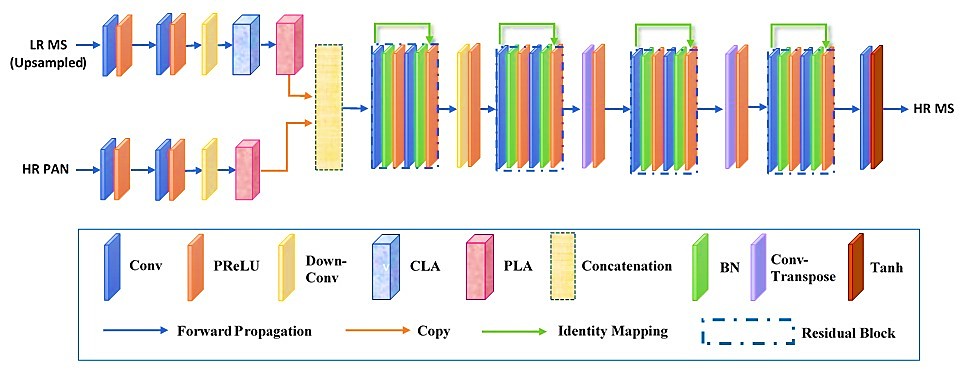
Figure 1: Detailed architecture of proposed dual attention-based two-stream pansharpening approach.

2.1 Feature Extraction

Similar to any vision task, pansharpening can use feature extraction methods from hand-crafted features to sparse encoding. However, the former are categorized as lossy transformations making it unsuitable for image reconstruction, while the latter requires a high-resolution image for dictionary creation and training. In contrast CNNs are capable of extracting image features, as well as, combining them in the feature domain.

2.2 Attention Mechanism

The resulting feature maps are processed using an attention mechanism to further enhance them. Recall that PAN and MS images contain different information, and hence, we design two types of attention mechanisms: pixel-level attention for PAN image and channel-level attention for MS image. Consequently, this assigns distinct weights to features at different levels before passing them to the feature fusion network.

Channel-level attention. recovers lost spatial information using a global mean pooling function (Fig. 2), formulated as:

$$\breve{G}_{c}=F_{c}(\breve{E}_{c})=\frac{1}{h\times w}\sum_{i=1}^{h}\sum_{j=1}^{w}{I_{c}(i,j)}$$ (1)

where $I_{c}(i,j)$ is the pixel at $(i,j)$ in channel $c$, and $F_{c}$ is the mean pooling function. The transformed feature map—from $(h\times w\times c)$ to $(1\times 1\times c)$—is fed to a dual-layer convolutional model with ReLU activation after each convolutional layer and sigmoid at the end, formulated as:

$$W_{c}=\sigma(conv(\Upsilon(conv(\breve{G}_{c}))))$$ (2)

where $\Upsilon$ and $\sigma$ demotes ReLU and sigmoid activations, respectively. The last step is element-wise multiplication of $\breve{G}(I_{M})$ and $W_{c}$ depicted as:

$$\breve{E}_{CLA}(I_{M})=\breve{E}(I_{M})\otimes W_{c}$$ (3)

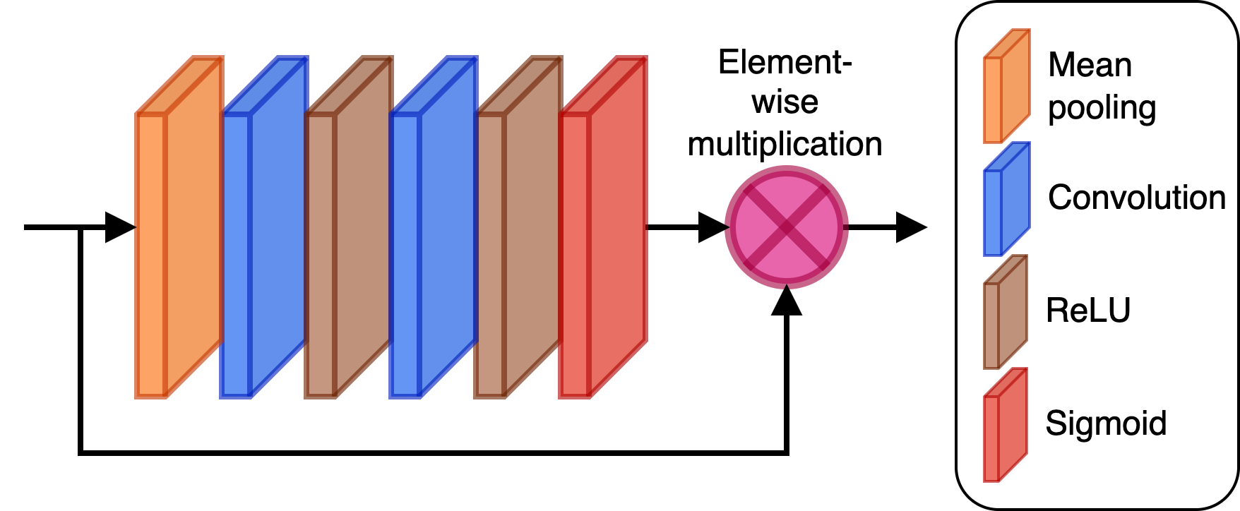
Figure 2: Layout of channel-level attention module.

Pixel-level attention. Similarly, information varies among different image pixels. We explicitly capture this information using a pixel-level attention (PLA) module. Here, the feature maps obtained from the PAN image feature extractor are fed to a dual-layer convolutional model with ReLU activation after each convolutional layer and sigmoid at the end as illustrated in Fig. 3. The model computes weights for distinct pixels as:

$$W_{p}=\sigma(conv(\Upsilon(conv(\breve{E}(I_{P})))))$$ (4)

The last step of this module is element-wise multiplication of $\breve{E}(I_{P})$ and $W_{P}$ depicted as:

$$\breve{E}_{PLA}(I_{P})=\breve{E}(I_{P})\otimes W_{P}$$ (5)

Figure 3: Layout of pixel-level attention module.

Notice that the PLA module is also applied to an MS image after CLA module to further enhance channel-level features.

2.3 Fusion Module

Once the feature maps are enhanced, the next step is their fusion. Generally, some pooling technique like mean or max pooling is used to fuse these feature maps, but this leads to information loss, contrary to the pansharpening task where every bit of information needs to be retained. To avoid this, we use an effective alternative for pooling that is concatenation, formulated as:

$$\breve{E}(I_{p},I_{M})=\breve{E}_{CLA}(I_{M})\oplus\breve{E}_{PLA}(I_{P})$$ (6)

where $\oplus$ denotes the concatenation, and $\breve{E}(I_{p},I_{M})$ is the fused feature map. This fused feature map acts as an input to the fusion network, which creates a more precise encoded representation of the concatenated features using three convolutional layers. The result is a tensor sized $[\frac{w}{4},\frac{h}{4},256]$, a compact encoding of spectral and spatial details of the MS and PAN images. This tensor is the input for the final reconstruction network used to reconstruct the pansharped image.

2.4 Reconstruction Network

The feature maps contain only one-fourth of the input in terms of height and width. Even though a simple linear interpolation technique can be used to match the spatial resolution requirement but a learnable approach would perform much better [9]. Here, we adopt a learnable approach for upsampling in terms of spatial resolution, a reconstruction network comprising transposed convolutional layers.

2.5 Skip Connections

To obtain a high quality pansharpened image, we include information from all levels of representation, but this increases the model’s computational complexity. To alleviate this, we use skip connection to copy feature maps from the encoder directly to the decoder after each upsampling phase, concatenating them to equivalent feature maps to infuse any lost details during downsampling. Here, we use a residual network (ResNet) to aid the flow of information from low-level layers to high-level layers. The network uses residual CNN units instead of simple CNN units, expressed as:

$$x_{n}=\hat{I}(r_{n})+\Omega(r_{n},\omega_{n});r_{n+1}=\phi(x_{n})$$ (7)

where $r_{n}$ and $r_{n+1}$ are input and output of ${n}^{th}$ residual CNN unit, $\Omega$ is residual function, $\hat{I}(r_{n})$ is identity mapping, and $\phi(x_{n})$ is activation.

2.6 Loss Function

The integral part of training a neural network is the loss function that computes the model error by evaluating a set parameter $(\vartheta)$. In the case of pansharpening the loss function also significantly affects the quality of pansharped image. Often $\ell_{2}$ norm is used as loss function for image-related tasks; however, this causes blurriness in the restored image. Instead, loss function $\ell_{1}$ is used for better training of image restoration models [10]. Likewise, we formulate the loss function $\ell_{1}$ for optimal training of the proposed network as:

$$\ell_{1}(\vartheta)=\frac{1}{n}\sum_{i=1}^{n}\mid\breve{E}(I_{P}^{i},I_{M}^{i};\vartheta)-X^{i}\mid_{1}$$ (8)

where $I_{P}$ is PAN image, $I_{M}$ is low-resolution MS image (LrMS) and $X$ is high-resolution MS image (HrMS), and $n$ is the training batch size.

3 Results

3.1 Experimental Dataset

Experiments are carried out on the Pléiades dataset. Images of two different locations: Toulouse and Strasbourg (France), are used for training and testing. These images contain trees, towns, roads, vegetation areas, water areas, and other kinds of land cover. The choice enables the evaluation of robustness of the proposed approach.

3.2 Evaluation Metrics

Recall that pansharpening fuses two images with different resolutions to obtain a single high-resolution image but due to the different dimensions, it introduces spectral and spatial distortions in the fused image. The robustness of the pansharpening method is evaluated by analyzing the fused image against the reference high-resolution MS image. Considering $\hat{H}$ is the fused image and $H$ is the reference image, both belonging to $\mathbb{R}^{M\times N}$, where $i$ and $j$ correspond to image row and column indices, and $\mu$ and $\sigma$ denote the mean and standard deviation of the images. The quality metrics used for evaluation are as follows:

1. Erreur relative globale adimensionnelle de synthèse (ERGAS). [11] measures image quality by taking normalized mean error of every band of fused image, given as:

   $$ERGAS=100\frac{dk}{dl}\sqrt{\frac{1}{n}\sum_{i=1}^{n}\left(\frac{RMSE_{i}}{mean_{i}}\right)^{2}}$$ (9)

   The ideal value is 0 whereas a higher value indicates distortions in the fused image.

2. Spectral angular mapper (SAM). [12] calculates the spectral angle between referenced image and fused image pixels. The metric measures the preserved spectral details by taking the mean of all the values, given as:

   $$SAM=\arccos\left(\frac{H_{j},\hat{H}_{j})}{\parallel H_{j}\parallel,\parallel\hat{H}_{j}\parallel}\right)$$ (10)

   Here, the output is either in radians or degrees with an ideal value of 0.

3. Universal image quality index (UIQI). [13] computes the transformation of known data from the original image into a pansharpened image, given as:

   $$UIQI=\frac{4\sigma_{\hat{H}H}(\mu_{H}+\mu_{\hat{H}})}{(\mu_{H}^{2}+\mu_{\hat{H}}^{2})(\mu_{H}^{2}+\mu_{\hat{H}}^{2})}$$ (11)

   The values range between -1 and 1, an ideal value of 1 for same images.

4. Spatial correlation coeficient (SCC). [14] assesses the spatial quality of pansharpened images. Here, the spatial details of pansharpened and reference images are extracted and then compared by computing a correlation coefficient between the extracted details. A Laplacian filter is computed band-by-band for detail extraction and correlation. The ideal value is 1 indicating spatial correlation between the two images.

5. Structural similarity index measure (SSIM). [15] is a similarity criterion between fused and reference images in terms of structure, contrast, and luminance, given as:

   $$SSIM=\frac{(2\mu_{H}\mu_{\hat{H}}+C_{1})(2\sigma_{H\hat{H}}+C_{2})}{({\mu_{H}}^{2}+{\mu_{\hat{H}}}^{2}+C_{1})({\mu_{H}}^{2}+{\mu_{\hat{H}}}^{2}+C_{2})}$$ (12)

The range of value is -1 to 1 with an ideal value of 1 representing similar images.

3.3 Methods for comparison

For comparison, we use several conventional methods including IHS [16], PCA [17], BDSD [18], PRACS [19], indusion [20], GLP [21], CBD [12], HPM [22] and HPM-PP [23]. From the DL domain, we use CAE [24] and TFNet [6].

3.4 Implementation details

There are 50,800 training image patches (LrMS, HR PAN, upsampled LrMS, and HrMS) of size 128$\times$128. The implementation is done using PyTorch on an NVIDIA GeForce GTX 980 GPU. The batch size is set to 32, adam optimizer is used for minimizing the loss with a 0.5 and 0.0001 momenta and learning rate, respectively. The model training takes around 12 hours.

3.5 Experimental analysis

We conduct two experiments to evaluate the performance of the proposed approach under different conditions. In first experiment, we consider the most favorable case of evaluation, where training and test images are of the same location taken by the same sensor. We use images of the Pléiades dataset representing urban areas of Toulouse and Strasbourg (France). Table I and II presents different quality metrics for different approaches including the proposed approach. Here, the low values of the first two metrics: ERGAS and SAM, indicate less distortion and spectral fidelity in the proposed approach, whereas the high value of UIQI and SSIM demonstrates that the learned features are similar to the reference image. Moreover, the ideal value achieved for SCC indicates that the pansharpened image from the proposed approach is spatially correlated to the reference image. TFNet also performs well producing better results compared to all conventional approaches. Notice that indusion method suffers from high distortion, meaning the technique lacks in its ability of feature representation.

TABLE I: List of quality metrics for a favorable case on Toulouse-Pléiades dataset.

Methods	ERGAS	SAM	UIQI	SCC	SSIM
IHS	3.005	0.111	0.983	0.665	0.848
PCA	2.882	0.105	0.984	0.666	0.859
BDSD	2.868	0.094	0.990	0.660	0.885
BT	3.0526	0.1137	0.9834	0.6665	0.840
GS	2.9697	0.1081	0.9827	0.6655	0.855
PRACS	2.419	0.080	0.992	0.665	0.882
HPF	3.7355	0.1367	0.9830	0.3475	0.713
Indusion	5.945	0.218	0.933	0.411	0.445
GLP	2.706	0.093	0.991	0.664	0.874
CBD	2.723	0.093	0.990	0.664	0.872
HPM	2.723	0.093	0.990	0.667	0.874
HPM-PP	3.027	0.106	0.988	0.662	0.857
CAE	2.856	0.092	0.985	0.626	0.868
TFNet	0.657	0.024	0.999	0.872	0.986
DATS	0.640	0.024	1.000	0.878	0.988

TABLE II: List of quality metrics for a favorable case on Strasbourg-Pléiades dataset.

Methods	ERGAS	SAM	UIQI	SCC	SSIM
IHS	1.639	0.063	0.997	0.452	0.754
PCA	1.431	0.054	0.997	0.454	0.905
BDSD	1.850	0.062	0.996	0.433	0.891
BT	1.7582	0.0669	0.9963	0.4534	0.7356
GS	1.4461	0.0509	0.9970	0.4543	0.8977
PRACS	1.414	0.048	0.997	0.456	0.913
HPF	2.2086	0.0747	0.9940	0.2167	0.7654
Indusion	4.041	0.1352	0.971	0.260	0.438
GLP	1.708	0.0593	0.997	0.446	0.834
CBD	1.707	0.0580	0.997	0.446	0.876
HPM	1.703	0.0593	0.997	0.445	0.834
HPM-PP	1.875	0.0652	0.996	0.445	0.823
CAE	2.540	0.0525	0.989	0.438	0.874
TFNet	0.708	0.0231	0.999	0.614	0.983
DATS	0.701	0.023	0.999	0.616	0.984

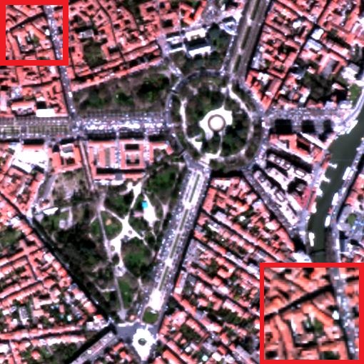
(a)

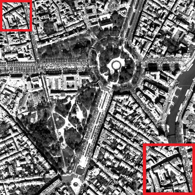
(b)

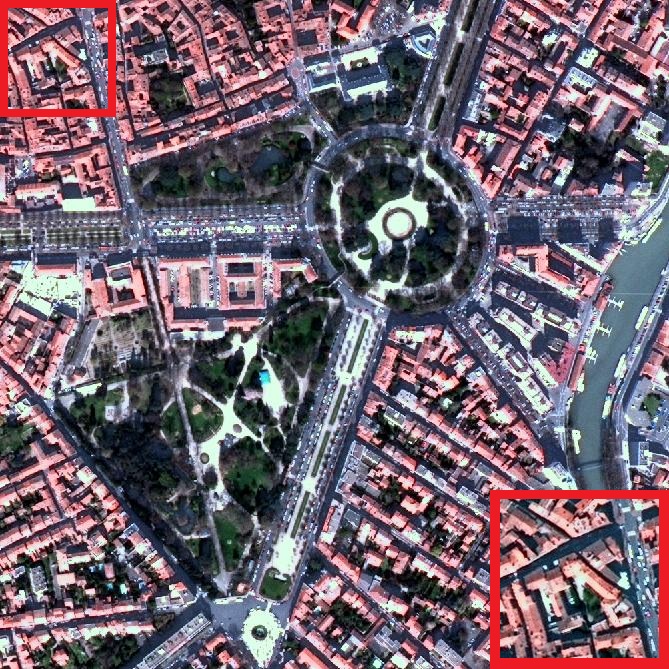
(c)

(d)

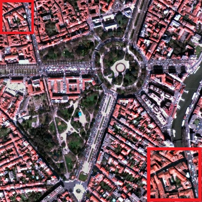
(e)

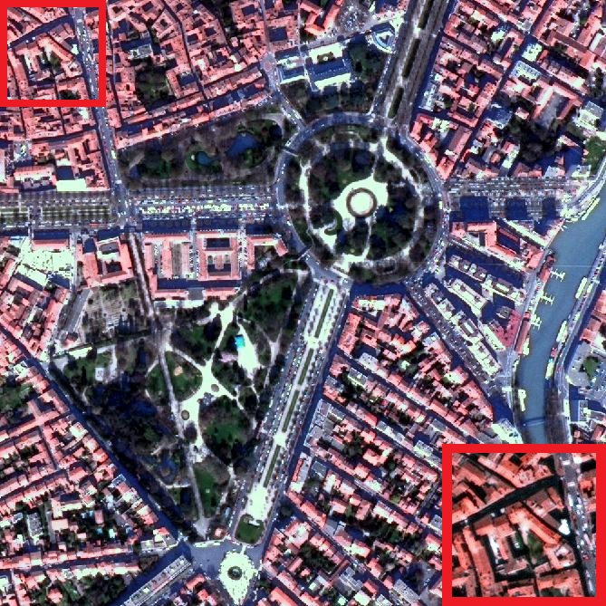
(f)

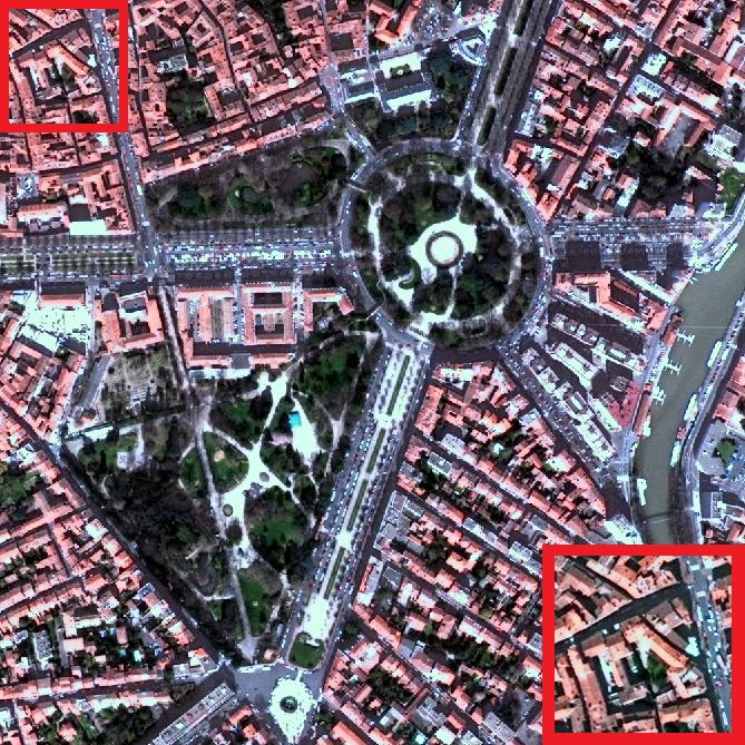
(g)

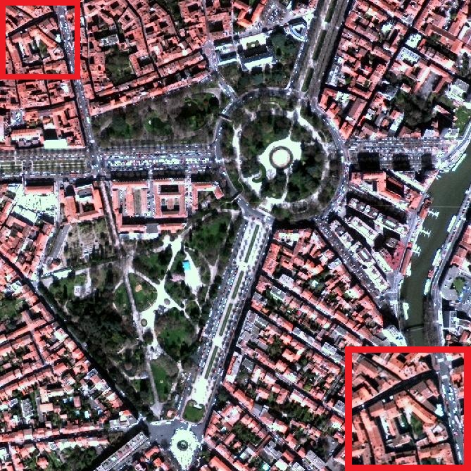
(h)

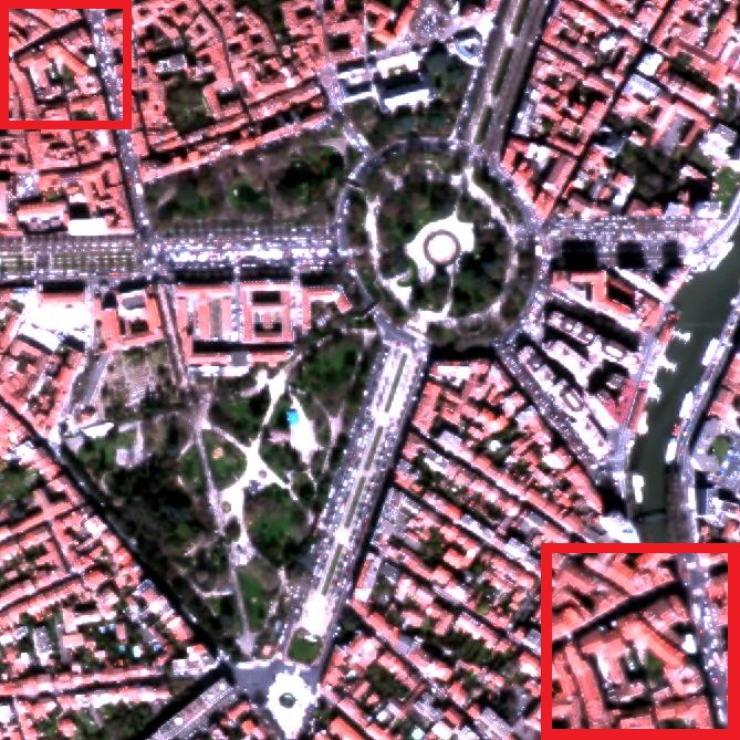
(i)

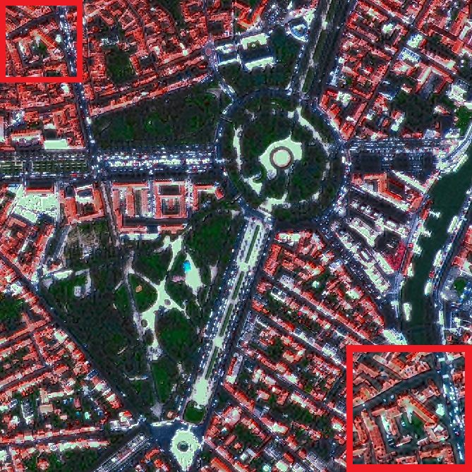
(j)

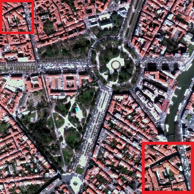
(k)

(l)

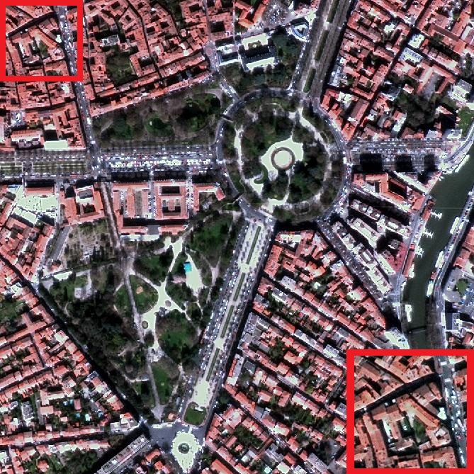
(m)

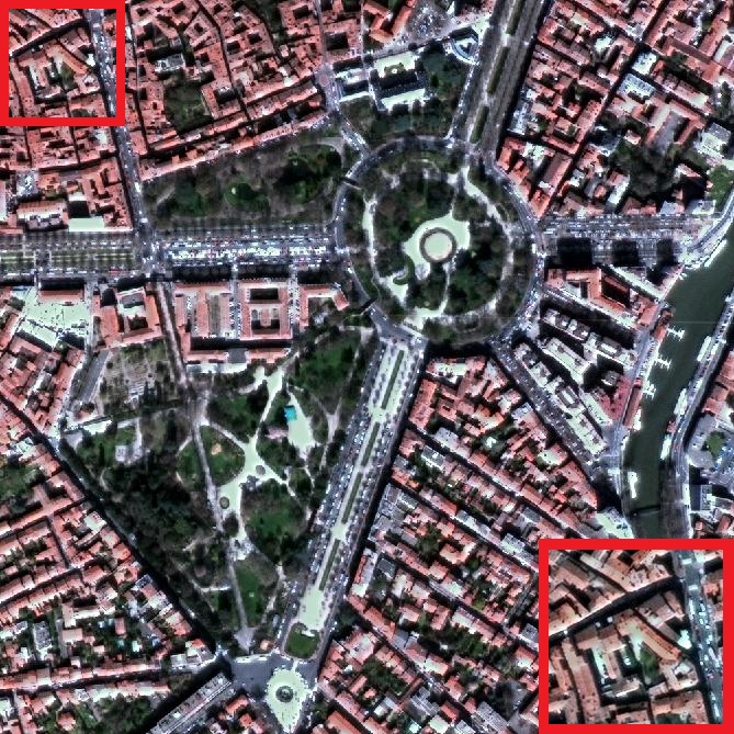
(n)

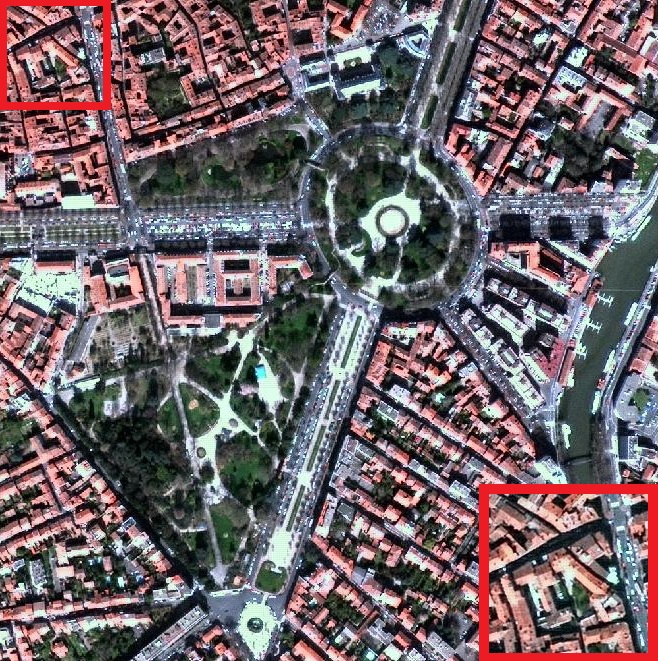
(o)

(p)

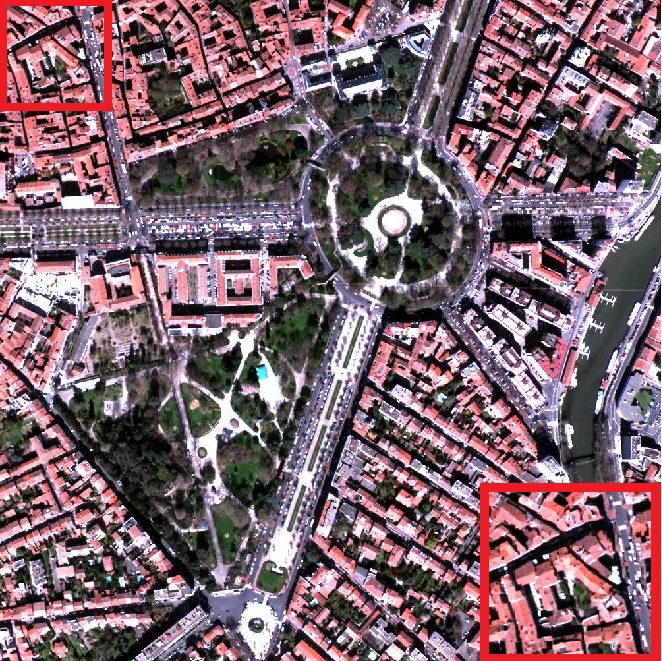
(q)

(r)

Figure 4: Visual results for Toulouse-Pléiades dataset. From top-left to bottom-right: LrMS, PAN, IHS, PCA, BDSD, BT, GS, PRACS, HPF, Indusion, MTF-GLP, MTF-GLP-CBD, MTF-GLP-HPM, MTF-GLP-HPM-PP, CAE, TFNet, DATS, and Reference.

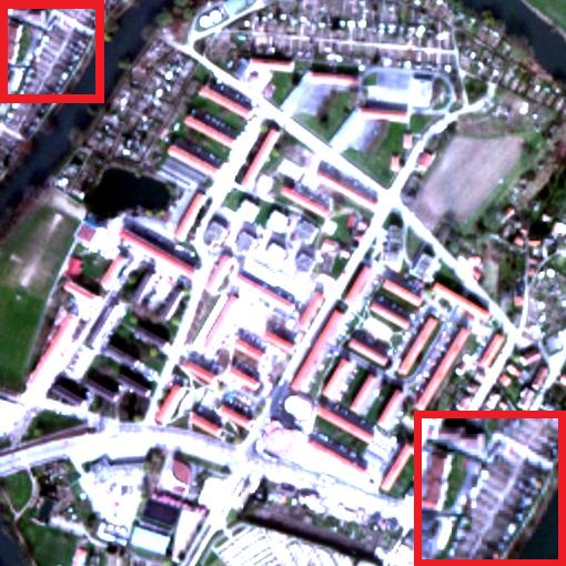
(a)

(b)

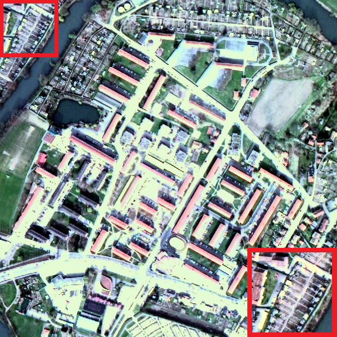
(c)

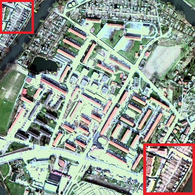
(d)

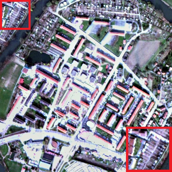
(e)

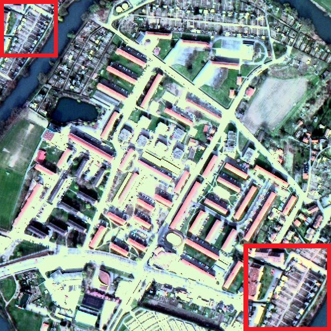
(f)

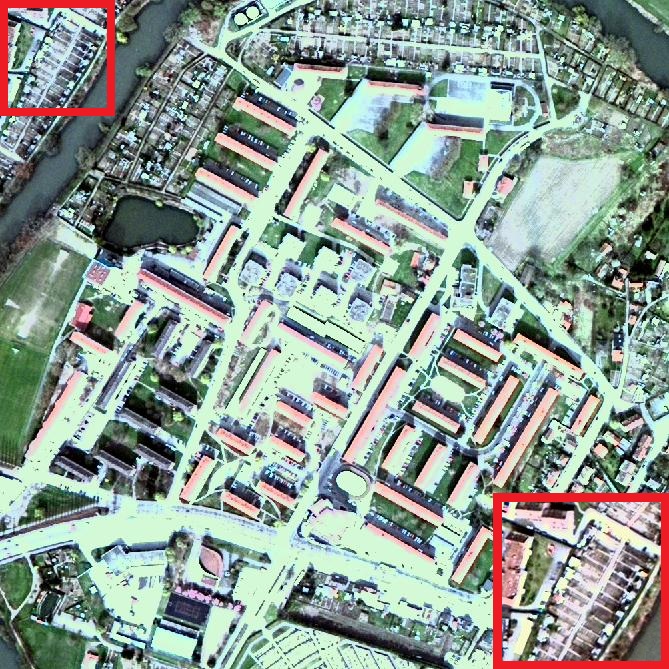
(g)

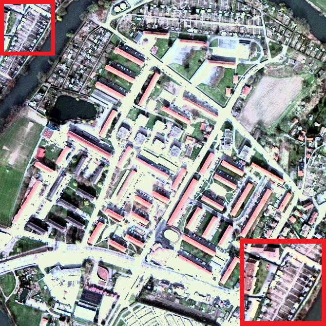
(h)

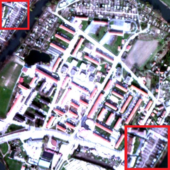
(i)

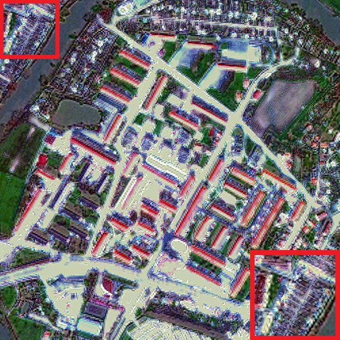
(j)

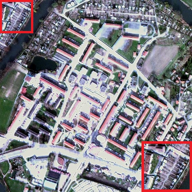
(k)

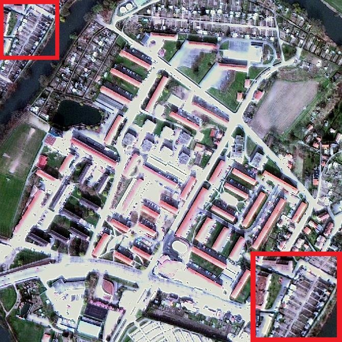
(l)

(m)

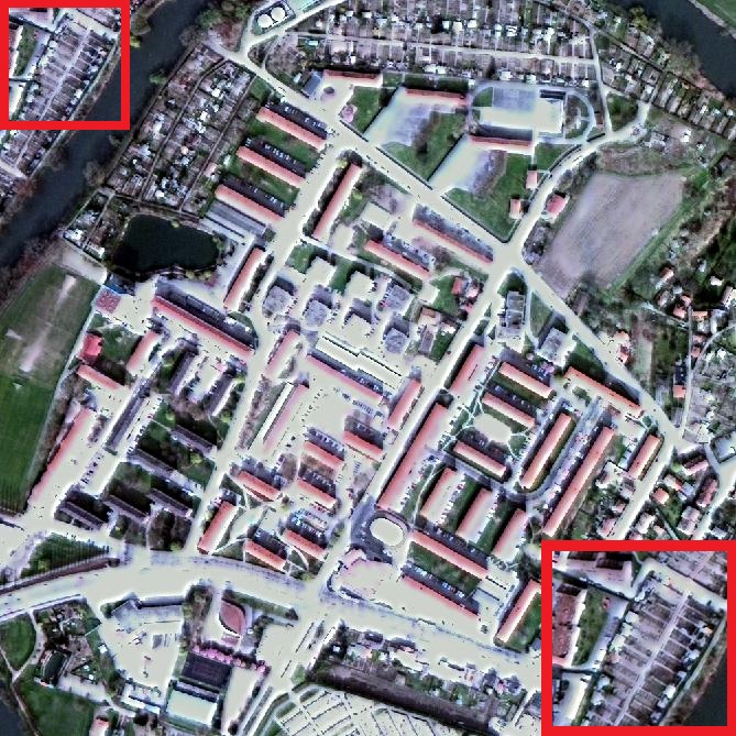
(n)

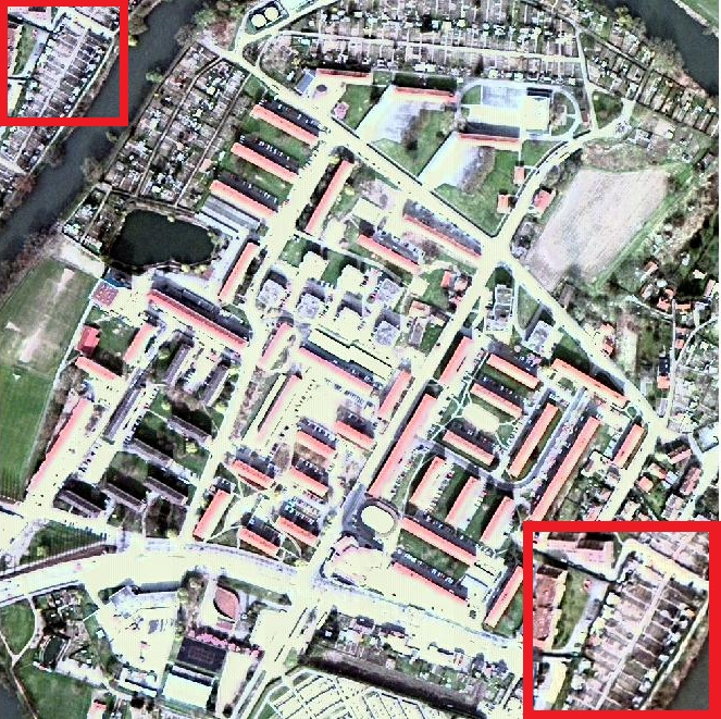
(o)

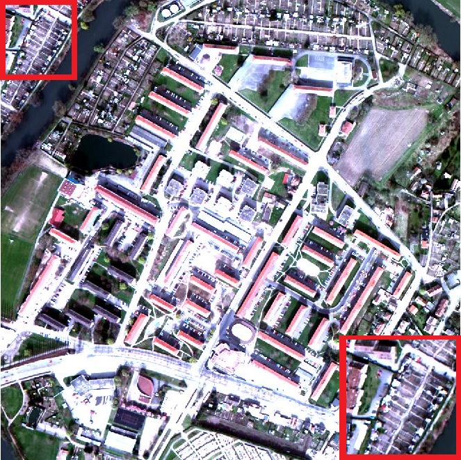
(p)

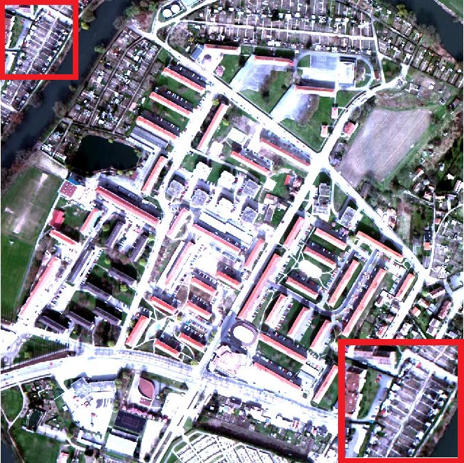
(q)

(r)

Figure 5: Visual results for Strasbourg-Pléiades dataset. From top-left to bottom-right: LrMS, PAN, IHS, PCA, BDSD, BT, GS, PRACS, HPF, Indusion, MTF-GLP, MTF-GLP-CBD, MTF-GLP-HPM, MTF-GLP-HPM-PP, CAE, TFNet, DATS, and Reference.

(a) LrMS

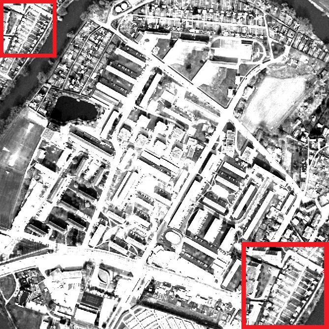
(b) PAN

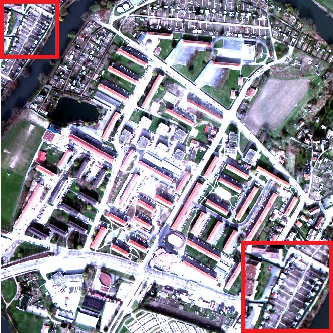
(c) TFNet

(d) DATS

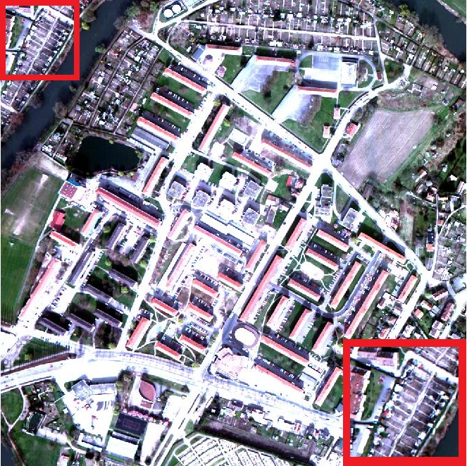
(e) Reference

Figure 6: Visual results of typical case on Pléiades dataset.

Fig. 4a and 5a present visual results of different pansharpening algorithms along with the proposed approach in false color synthesis (3 bands as 3, 2, 1). From visual analysis, we observe that the most recent DL-based methods TFNet and DATS are robust in learning sensor characteristics and preserving underlying spectral details while enhancing desired spatial details. They also depict efficiency in terms of image registration and feature learning. However, IHS produced a pansharped image with suitable spatial fidelity but with much spectral distortion. Again the resultant image of indusion suffers from the most distortion whereas BDSD lacks spatial details. Moreover, the visual output of HPM is better compared to its variant HPM-PP. Other approaches including PRACS and GLP achieve promising results among the conventional approaches.

In the second experiment, we consider a typical case of evaluation where training and test images are taken by the same sensor but of different locations. We use images of the Pléiades dataset representing urban areas of Toulouse and Strasbourg (France), the first image set for training while the second for testing. Notably, this evaluation helps determine the effectiveness of the DL models to learn sensor degradation. Table III presents the quality metrics computed for TFNet and the proposed approach along with ideal values for a typical case. The low ERGAS and SAM values for the proposed approach indicate less distortion and high spectral correlation. While the high values of UIQI, SCC and SSIM in the case of the proposed approach shows the model’s proficiency learning features for the respective sensor. This results in pansharpened images that are spatially correlated to the reference image.

TABLE III: List of computed quality metrics for a typical case along with their ideal values.

Methods	ERGAS	SAM	UIQI	SCC	SSIM
Reference	0	0	1	1	1
TFNet	0.735	0.025	0.999	0.588	0.980
DATS	0.735	0.025	0.999	0.593	0.980

Fig. 6a presents visual results for TFNet and DATS in false color synthesis (3 bands as 3, 2, 1). From visual inspection, we observe the efficacy of the two DL-based methods to extract representative features, to learn fundamental characteristics of sensors, and to preserve underlying spectral fidelity while enhancing required spatial information without manual intervention.

4 Conclusions

We present a novel dual attention-based two-stream (DATS) pansharpening method that fuses an HR PAN and LrMS image and delivers a pansharped MS image high in both spatial and spectral information. The computed quality measures confirm that the proposed approach can efficiently learn the degradation process of the corresponding sensor and can effectively produce a pansharped image having high spatial details while maintaining the spectral fidelity of the underlying image. In the future, we will explore the transability of our proposed network among different sensors.

References

- [1] G. Masi, D. Cozzolino, L. Verdoliva, and G. Scarpa, “Pansharpening by convolutional neural networks,” Remote Sens., vol. 8, no. 7, p. 594, 2016.
- [2] L. He, Y. Rao, J. Li, J. Chanussot, A. Plaza, J. Zhu, and B. Li, “Pansharpening via detail injection based convolutional neural networks,” IEEE J. Sel. Top. Appl. Earth Obs. Remote Sens., vol. 12, no. 4, pp. 1188–1204, 2019.
- [3] Q. Yuan, Y. Wei, X. Meng, H. Shen, and L. Zhang, “A multiscale and multidepth convolutional neural network for remote sensing imagery pan-sharpening,” IEEE J. Sel. Top. Appl. Earth Obs. Remote Sens., vol. 11, no. 3, pp. 978–989, 2018.
- [4] W. Huang, X. Fei, J. Yin, and Y. Liu, “A multi-direction subbands and deep neural networks bassed pan-sharpening method,” in IEEE Int. Geosci. Remote Sens. Symp. (IGARSS), 2018, pp. 5139–5142.
- [5] G. He, S. Xing, Z. Xia, Q. Huang, and J. Fan, “Panchromatic and multi-spectral image fusion for new satellites based on multi-channel deep model,” Mach. Vision Appl., vol. 29, no. 6, pp. 933–946, 2018.
- [6] X. Liu, Q. Liu, and Y. Wang, “Remote sensing image fusion based on two-stream fusion network,” Inf. Fusion, vol. 55, pp. 1–15, 2020.
- [7] M. Jiang, H. Shen, J. Li, Q. Yuan, and L. Zhang, “A differential information residual convolutional neural network for pansharpening,” ISPRS J. Photogramm. Remote Sens., vol. 163, pp. 257–271, 2020.
- [8] X. Li, F. Xu, X. Lyu, Y. Tong, Z. Chen, S. Li, and D. Liu, “A remote-sensing image pan-sharpening method based on multi-scale channel attention residual network,” IEEE Access, vol. 8, pp. 27 163–27 177, 2020.
- [9] J. Long, E. Shelhamer, and T. Darrell, “Fully convolutional networks for semantic segmentation,” in IEEE/CVF Conf. Comput. Vision Pattern Recognit. (CVPR), 2015, pp. 3431–3440.
- [10] B. Lim, S. Son, H. Kim, S. Nah, and K. Mu Lee, “Enhanced deep residual networks for single image super-resolution,” in IEEE/CVF Conf. Comput. Vision Pattern Recognit. (CVPR). workshops, 2017, pp. 136–144.
- [11] C. Zhang, Q. Yan, Y. Zhu, X. Li, J. Sun, and Y. Zhang, “Attention-based network for low-light image enhancement,” in IEEE Int. Conf. Multimedia Expo (ICME), 2020, pp. 1–6.
- [12] L. Alparone, L. Wald, J. Chanussot, C. Thomas, P. Gamba, and L. M. Bruce, “Comparison of pansharpening algorithms: Outcome of the 2006 grs-s data-fusion contest,” IEEE Trans. Geosci. Remote Sens., vol. 45, no. 10, pp. 3012–3021, 2007.
- [13] Z. Shi, C. Chen, Z. Xiong, D. Liu, Z.-J. Zha, and F. Wu, “Deep residual attention network for spectral image super-resolution,” in Eur. Conf. Comput. Vision (ECCV) Workshops, 2018.
- [14] X. Otazu, M. González-Audícana, O. Fors, and J. Núñez, “Introduction of sensor spectral response into image fusion methods. application to wavelet-based methods,” IEEE Trans. Geosci. Remote Sens., vol. 43, no. 10, pp. 2376–2385, 2005.
- [15] Q. Yang, Y. Xu, Z. Wu, and Z. Wei, “Hyperspectral and multispectral image fusion based on deep attention network,” in 10th Workshop Hyperspectral Image Signal Process.: Evol. Remote Sens. (WHISPERS), 2019, pp. 1–5.
- [16] T.-M. Tu, S.-C. Su, H.-C. Shyu, and P. S. Huang, “A new look at ihs-like image fusion methods,” Inf. Fusion, vol. 2, no. 3, pp. 177–186, 2001.
- [17] P. Kwarteng and A. Chavez, “Extracting spectral contrast in landsat thematic mapper image data using selective principal component analysis,” Photogramm. Eng. Remote Sens, vol. 55, no. 1, pp. 339–348, 1989.
- [18] A. Garzelli, F. Nencini, and L. Capobianco, “Optimal mmse pan sharpening of very high resolution multispectral images,” IEEE Trans. Geosci. Remote Sens., vol. 46, no. 1, pp. 228–236, 2007.
- [19] J. Choi, K. Yu, and Y. Kim, “A new adaptive component-substitution-based satellite image fusion by using partial replacement,” IEEE Trans. Geosci. Remote Sens., vol. 49, no. 1, pp. 295–309, 2010.
- [20] M. M. Khan, J. Chanussot, L. Condat, and A. Montanvert, “Indusion: Fusion of multispectral and panchromatic images using the induction scaling technique,” IEEE Geosci. Remote Sens. Lett., vol. 5, no. 1, pp. 98–102, 2008.
- [21] B. Aiazzi, L. Alparone, S. Baronti, A. Garzelli, and M. Selva, “Mtf-tailored multiscale fusion of high-resolution ms and pan imagery,” Photogramm. Eng. Remote Sens., vol. 72, no. 5, pp. 591–596, 2006.
- [22] G. Vivone, R. Restaino, M. Dalla Mura, G. Licciardi, and J. Chanussot, “Contrast and error-based fusion schemes for multispectral image pansharpening,” IEEE Geosci. Remote Sens. Lett., vol. 11, no. 5, pp. 930–934, 2013.
- [23] J. Lee and C. Lee, “Fast and efficient panchromatic sharpening,” IEEE Trans. Geosci. Remote Sens., vol. 48, no. 1, pp. 155–163, 2009.
- [24] A. Azarang, H. E. Manoochehri, and N. Kehtarnavaz, “Convolutional autoencoder-based multispectral image fusion,” IEEE Access, vol. 7, pp. 35 673–35 683, 2019.