Niobium in clean limit: an intrinsic type-I superconductor

Abstract

Niobium is one of the most researched superconductors, both theoretically and experimentally. It is enormously significant in all branches of superconducting applications, from powerful magnets to quantum computing. It is, therefore, imperative to understand its fundamental properties in great detail. Here we use the results of recent microscopic calculations of anisotropic electronic, phonon, and superconducting properties, and apply thermodynamic criterion for the type of superconductivity, more accurate and straightforward than a conventional Ginzburg-Landau parameter $\kappa$ - based delineation, to show that pure niobium is a type-I superconductor in the clean limit. However, disorder (impurities, defects, strain, stress) pushes it to become a type-II superconductor.

I Introduction

Niobium metal is one of the most important materials for superconducting technologies, from SRF cavities [1], to superconducting circuits for sensitive sensing [2] and quantum informatics [3]. Numerous experimental works report measurements on different samples, from almost perfect single crystals to disordered films [4, 5, 6, 7, 3, 8, 9, 10, 11, 12]. Likewise, numerous theories explore its properties from microscopic calculations to phenomenological theories [13, 14, 15, 16, 1, 17, 18, 19]. It is impossible to acknowledge a multitude of relevant references, so we will limit ourselves to the specific topic of the paper.

Despite various attempts, first-principle calculations of the absolute values of the critical fields, in particular the upper critical field, $H_{c2}$, remain in poor agreement with the experiment. As a result, either the temperature dependence of the normalized field, usually as introduced by Helfand and Werthamer, $h^{*}\equiv H_{c2}\left(T\right)/T_{c}H^{\prime}_{c2}\left(T=T_{c}\right)$ [20], is calculated [21], or calculations use experimental parameters, such as Fermi velocities, $v$, to fit the data [15]. Considering that $H_{c2}\sim v^{-2}$, this makes a significant difference. As we show in this paper, this is no fault of the theorists, but rather quite ambiguous experimental determination of the critical fields. This, in turn, is no fault of the experimentalists, because it is clear that Nb is extraordinarily susceptible to the disorder with its experimental $RRR\equiv R\left(300\>\text{K}\right)/R\left(T_{c}\right)$, ranging between $3$ and $90000$ [4, 9].

Previously, the problem of the identification of the type of superconductivity was analyzed in detail at arbitrary temperatures [22, 23]. It was argued that instead of a conventional criterion based on the Ginzburg-Landau parameter, $\kappa=\lambda/\xi$, one has to use the ratio of the upper and thermodynamic critical fields, $h_{c2,c}\equiv H_{c2}/H_{c}$. Alternatively, it could be the ratio of $h_{c,c1}\equiv H_{c}/H_{c1}$, but superheating [24, 25] and various surface barriers [26, 27] make experimental determination of the lower critical field, $H_{c1}$, difficult. Only when $h_{c2,c}>1$, do vortices form and the material can be identified as a type-II superconductor. As it is shown in Ref. [22, 23], the $\kappa-$based criterion coincides with the thermodynamic criterion only at $T_{c}$, and not even within a small temperature interval below $T_{c}$. In other words, the slopes of the temperature-dependent $h_{c2,c}\left(T\right)$ and $\kappa\left(T\right)$ are different at $T_{c}$. In anisotropic superconductors, the same sample can be type-I in one orientation of the magnetic field, and type-II in another [22].

Of course, in the case of significantly different $\lambda$ and $\xi$, the difference between the two criteria is not that important and this is why the type of most superconductors was correctly identified using the Ginzburg-Landau parameter $\kappa$. Moreover, it is well known that there are practically no proven non-elemental type-I superconductors, except for a few suggested compounds, such as Ag₅Pb₂O₆ [28], YbSb₂ [29], OsB₂ [30], and PdTe₂ [31]. However, until the intermediate state is directly observed instead of a mixed state of Abrikosov vortices by magneto-sensitive imaging techniques, the type-I status of these materials will remain “pending”.

Niobium seems to be a difficult case, because, by all accounts, it is situated close to the crossover boundary and can be easily moved deeper into the type-II side by non-magnetic disorder, which increases the London penetration depth, $\lambda$, and decreases the coherence length, $\xi$. Magnetic disorder, on the other hand, pushes a superconductor into the opposite direction Recently high-quality magneto-optical imaging of Nb single crystals with $RRR=500$ has revealed directly and unambiguously a clear structure of the intermediate state [12]. These images are strikingly similar to images by one of us (RP) for the commonly accepted type-I superconductor, pure lead [32, 33, 34]. So similar that the authors of Ref.[12] write in their paper, “The observed patterns of the IMS [intermediate mixed state] are rather similar to that of the Meissner and normal domains in the intermediate state of the type-I superconductor, Pb reported by Prozorov et al. [32, 33]”. This is, indeed, the case.

The tendency to type-I behavior of elemental metals is not unique to niobium. A clear cross-over from a type-I (confirmed by magneto-optical imaging [35]) to a type-II regime upon introduction of non-magnetic scattering was convincingly demonstrated in tantalum [35, 36]. In known type-II vanadium, the Ginzburg-Landau parameter $\kappa$ approaches the borderline value of $1/\sqrt{2}$ toward type-I behavior with the increase of the residual resistivity ratio [37].

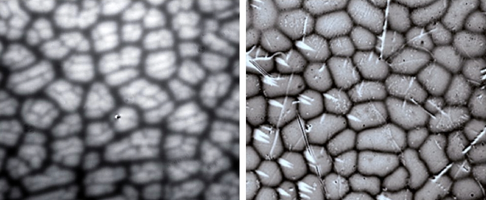
Figure 1: (Left) the intermediate state in a single crystal Nb (Ref.[12], Fig.3a). (Right) the intermediate state in a single crystal Pb, (Ref.[33], Fig.2g). [Left frame reprinted with permission from: S. Ooi, M. Tachiki, T. Konomi, T. Kubo, A. Kikuchi, S. Arisawa, H. Ito, and K. Umemori, “Observation of Intermediate Mixed State in High-Purity Cavity-Grade Nb by Magneto-Optical Imaging”, Physical Review B 104, 6 (2021). Copyright (2021) by the American Physical Society]

Figure 1 compares the intermediate state structure in niobium and lead single crystals. The visual similarity is remarkable. Of course, depending on the material, its properties and the proximity to the crossover boundary the fine details vary. For example, here the field-cooled (FC) image is shown for Nb, and zero-field-cooled is shown for Pb. Upon field cooling, the intermediate state in Pb breaks into a corrugated laminar structure, whereas in Nb it apparently further breaks into large flux tubes, only reinforcing our earlier conclusion that the equilibrium topology of the intermediate state in type-I superconductors is tubular, rather than laminar [32]. Since the textbooks tell us that the true intermediate state structure is described as laminar, stripy, or labyrinth-like, the observation of the tubular features was often interpreted as some kind of crossover “intermediate mixed state” when vortices gather into “domains” as illustrated in Fig.4e of Ref.[12]. However, no evidence of individual vortices was found in such structures. For a variety of magneto-optical images of superconductors, the reader is referred to Ref. [38]. In our interpretation, the authors of Ref.[12] have observed a genuine intermediate state in a clean-limit Nb crystal proving experimentally that Nb is a type-I superconductor. We now check whether the microscopic theory agrees.

II Properties of niobium from the microscopic theory

Recently, based on the density functional theory (DFT) calculations of the electron and phonon band structures, microscopic superconducting properties of elemental niobium were determined using Eliashberg formalism [19]. It was found that pure Nb is a two-active-bands, two-gap superconductor. The bands are moderately anisotropic with temperature-dependent anisotropies. The more isotropic band 2 dominates the electronic properties. For analytical estimates, we use isotropic BCS formulas, but then we use 2-band averaged RMS values from Ref. [19]. Specifically, $v=\sqrt{\left\langle v^{2}\right\rangle}$, the RMS value of the Fermi velocity is given by, $v=\sqrt{n_{1}v_{1}^{2}+n_{2}v_{2}^{2}}$, where partial densities of states (DOS), $n_{1,2}=N_{1,2}(0)/\left(N_{1}+N_{2}\right)$, and a similar equation was used for the RMS superconducting gap. We compare analytical results with the full numeric evaluation of anisotropic equations. The paper uses cgs units throughout. We calculate critical fields analytically at $T=0$ and $T=T_{c}$ and their ratios and compare them with the Ginzburg-Landau criterion for the type of a superconductor.

Here we summarize the parameters used from Ref.[19]. The densities of states at the Fermi level: $N_{1}(0)=6.33$$\times 10^{33}$ erg^-1cm^-3, $N_{2}(0)=3.98$$\times 10^{34}$ erg^-1cm^-3, $N_{tot}(0)=4.61$$\times 10^{34}$ erg^-1cm^-3. The averaged RMS velocities, $,v_{1}=4.37$$\times 10^{7}$ cm/s, $v_{2}=7.62$$\times 10^{7}$ cm/s, and 2-band average, $v=7.26\times 10^{7}cm/s$. The RMS averaged superconducting gaps, $\varDelta_{1}\left(0\right)=3.14\times 10^{-15}$ erg, $\varDelta_{2}\left(0\right)=2.53\times 10^{-15}$ erg, and $\varDelta\left(0\right)=2.62\times 10^{-15}$ erg . For comparison, the weak-coupling BCS gap is $\varDelta_{BCS}\left(0\right)=1.7638T_{c}=2.27\times 10^{-15}$ erg with $T_{c}=9.33$ K. The Fermi energy of Nb is $E_{F}=5.32$ eV $=8.52\times 10^{-12}$ erg [39]. The total carrier density is $n=5.56\times 10^{22}$ cm^-3 and the effective electron mass is $m^{*}=2.14m_{e}$ [13]. Note that two-bands averaged values are very close to band 2 values, reflecting its dominant character.

Let us now estimate various quantities using analytic limiting cases from the BCS theory. The upper critical field at $T=0$ is given by [20],

$$H_{c2}\left(0\right)=\frac{\phi_{0}}{2\pi\xi^{2}}=\frac{\phi_{0}\pi k_{B}^{2}T_{c}^{2}}{2\hbar^{2}v^{2}}\exp\left(2-C\right)$$

where $C=0.577216$ is the Euler constant. Technically, two bands will have two different characteristic coherence lengths [40]. Of course, there is only one upper critical field, but a formal substitution of bands’ Fermi velocities gives $H_{c2}\left(0\right)=1053$ Oe and $346$ Oe for bands 1 and 2, respectively. These values are far from the reported values of $3-5$ kOe [21, 15, 4]. For the 2-band average, $H_{c2}\left(0\right)=381$ Oe. The coherence lengths formally corresponding to these fields, are $\xi\left(0\right)=56$ nm and $97$ nm for bands 1 and 2, respectively, and $\xi\left(0\right)=93$ nm for the two-band average. For comparison, the BCS coherence length is:

$$\xi_{0}=\frac{\hbar v}{\pi\varDelta\left(0\right)}$$

which gives $\xi_{0}=47$ nm and $101$ nm for bands 1 and 2, respectively, and $\xi_{0}=98$ nm for the 2-band average.

The thermodynamic critical field is given by

$$H_{c}\left(0\right)=2\sqrt{\pi N\left(0\right)}\sqrt{\left\langle\varDelta^{2}\left(0\right)\right\rangle}$$

and we obtain $H_{c}\left(0\right)=1993$ Oe. Note a substantial difference between this value and the much lower “upper” critical fields above. On the other hand, this field scale is quite close to what was determined as experimental critical fields in clean samples [4, 14], considering that it is very difficult to distinguish hysteresis loops of relatively pure niobium and, for example, lead with some pinning [32].

III Type-I superconductivity in clean-limit niobium metal

According to Ref.[22], the natural way to determine the type of a superconductor is to examine the ratio of $h_{c2,c}\equiv H_{c2}/H_{c}$. While Ref.[22], provides a recipe for calculating this ratio at all temperatures, here we only need to consider $T=0$ and $T=T_{c}$ for which analytic expressions are available. If the gap anisotropy is described by the order parameter, $\varDelta\left(T,k\right)=\Psi\left(T\right)\Omega\left(k\right)$, where the angular part is normalized over Fermi surface average, $\left\langle\Omega^{2}\right\rangle=1$, then for the magnetic field along the $c-$axis [22],

$$h_{c2,c}\left(0\right)=\frac{\phi_{0}k_{B}T_{c}}{\hbar^{2}v_{0}^{2}\sqrt{\pi N\left(0\right)}}\exp\left\langle\Omega^{2}\ln\frac{\left|\Omega\right|}{\mu_{z}}\right\rangle$$ (1)

where $\mu_{z}=\left(v_{x}^{2}+v_{y}^{2}\right)/v_{0}^{2}$, and $v_{0}$ is the characteristic velocity scale (equal to Fermi velocity in isotropic case),

$$v_{0}=\left(\frac{2E_{F}^{2}}{\pi^{2}\hbar^{3}N\left(0\right)}\right)^{1/3}$$

For band 2, we have: $v_{0,2}=6.81$$\times 10^{7}$ cm/s and using total DOS, $v_{0,tot}=6.48$$\times 10^{7}$ cm/s. In particular, for the isotropic case, $\left\langle\mu_{c}\right\rangle=2/3$, and $\left\langle\ln\mu_{c}\right\rangle=2\left(\ln 2-1\right)$, which then reproduces Helfand-Werthamer result [20],

$$h_{c2,c}\left(0\right)=\frac{\phi_{0}k_{B}T_{c}}{\hbar^{2}v_{0}^{2}\sqrt{\pi N\left(0\right)}}\exp\left(-2\left(\ln 2-1\right)\right)$$

Using the two-band average, we obtain, $h_{c2,c}^{2bands}\left(0\right)=0.221$, while using only band 2 we obtain $h_{c2,c}^{band2}\left(0\right)=0.216$.

For $T\rightarrow T_{c}$ we have in general:

$$h_{c2,c}\left(T_{c}\right)=\frac{3\sqrt{2}\phi_{0}k_{B}T_{c}}{\hbar^{2}v_{0}^{2}\sqrt{7\zeta\left(3\right)\pi N\left(0\right)}}\frac{\sqrt{\left\langle\Omega^{4}\right\rangle}}{\left\langle\Omega^{2}\mu_{z}\right\rangle}\,$$ (2)

where $\zeta\left(3\right)=1.2021$ is Riemann’s zeta function. In the isotropic case this reduces to,

$$h_{c2,c}\left(T_{c}\right)=\frac{3\sqrt{2}\phi_{0}k_{B}T_{c}}{\hbar^{2}v_{0}^{2}\sqrt{7\zeta\left(3\right)\pi N\left(0\right)}}$$

For the two-band average we obtain $h_{c2,c}^{2bands}\left(T_{c}\right)=0.175$, and for band 2, $h_{c2,c}^{band2}\left(T_{c}\right)=0.171$. Looking at the previous two equations it is easy to see that their ratio is a pure number, $h_{c2,c}\left(0\right)/h_{c2,c}\left(T_{c}\right)=1.263$, independent of material properties. However, the ratio does depend on the anisotropy of the Fermi surface and of the order parameter via Fermi surface averages of the terms containing functions of $\Omega(k)$. Indeed the result for the Fermi surface average appearing in Eq. (1) based on the bandstructure and Eliashberg results for the Fermi velocity and anisotropic gap function at $T/T_{c}=0.32$ yield,

$$\left\langle\Omega^{2}\,\ln\left(\frac{|\Omega|}{\mu_{z}}\right)\right\rangle=0.98\,,$$ (3)

which gives $h_{c2,c}(0)\approx 0.319$. Thus, pure, single-crystaline Nb is in the Type I limit based first-principles calculations of the gap and Fermi surface anisotropy [19].

An additional method to verify the consistency of the above analysis is to use the fact that at $T=T_{c}$ [22],

$$h_{c2,c}\left(T_{c}\right)=\sqrt{2}\kappa_{GL}$$

where Ginzburg-Landau $\kappa_{GL}$ is given by,

$$\kappa_{GL}=\frac{3\phi_{0}k_{B}T_{c}}{\hbar^{2}v^{2}\sqrt{7\zeta\left(3\right)\pi N\left(0\right)}}$$

Evaluating for two bands average, we obtain at $T_{c}$, $\kappa_{GL}=0.123$ and then, indeed $\sqrt{2}\kappa_{GL}=0.175=h_{c2,c}\left(T_{c}\right)$. In another limit, $T=0$, we can evaluate $\kappa\left(0\right)=\lambda\left(0\right)/\xi\left(0\right)$. In the isotropic approximation, the London penetration depth becomes,

$$\lambda\left(0\right)=\frac{c}{e}\sqrt{\frac{m^{*}}{4\pi n}}\approx 33\>\mathrm{nm}$$

Thus,

$$\kappa\left(0\right)=\frac{33\>\mathrm{nm}}{93\>\mathrm{nm}}=0.355<\frac{1}{\sqrt{2}}=0.71$$

Therefore, even this simple estimate based on isotropic London theory gives the value of $\kappa$ corresponding to type-I superconductivity. A more straightforward thermodynamic criterion based on the ratio of the critical fields gives the values of $h_{c2,c}$ clearly lower than one, which places niobium in the domain of type-I superconductivity. The situation, however, quickly changes with the addition of non-magnetic scattering. The upper critical field grows linearly with the scattering rate [40, 41, 42] and quickly exceeds $H_{c}$. Magnetic impurities, on the other hand, would bring $H_{c2}$ down, but they will also suppress $T_{c}$ [41, 23].

For applications of SRF cavities for particle accelerator technology it is desirable to stabilize Nb closer to a type-I phase where one can increase the superheating field by engineering the disorder profile very close to the superconducting-vacuum interface, leaving much of the London penetration region in the clean limit [43, 44]. In quantum informatics where thin films are used, perhaps switching to the epitaxial growth instead of ablation-type sputtering would improve the RRR, and hence improved device performance.

IV Conclusions

It is shown that using the parameters of recent microscopic calculations of superconducting and electronic properties of pure Nb, the estimated ratio of the upper and thermodynamic critical fields, $H_{c2}/H_{c}$, changes from 0.22 at $T=0$, to 0.18 at $T_{c}$. These values place clean-limit niobium squarely into the domain of type-I superconductivity. This conclusion is firmly supported by the direct magneto-optical observation of the intermediate state in Nb single crystals with RRR=500 [12]. It is suggested that ever-present disorder and impurities drive the real material to a type-II side in most samples studied by experimentalists so far.