Optimal data generation for machine learned interatomic potentials

Abstract

MLIP are routinely used atomic simulations, but generating databases of atomic configurations used in fitting these models is a laborious process, requiring significant computational and human effort. A computationally efficient method is presented to generate databases of atomic configurations that contain optimal information on the small-displacement regime of the PES of bulk crystalline matter. Utilising NDSCLloyd-Williams and Monserrat (2015), an automatic process is suggested for ab initio data generation. MLIP were fitted for Al, W, Mg and Si, which very closely reproduce the ab initio phonon and elastic properties. The protocol can be easily adapted to other materials and can be inserted in the workflow of any flavour of MLIP generation.

UK Ministry of Defence © British Crown Owned Copyright 2022/AWE

I Introduction

Modern approaches to material discovery and characterisation include the use of ab initio modelling. While well-established methods, such as DFT, reliably predict the electronic, mechanic and thermodynamic properties of materialsPickard and Needs (2006, 2011), most of these techniques are limited by the fact that computational effort scales as $\mathcal{O}(N^{3})$ or worse with the number of atoms ($N$). Although linear scaling implementations of DFT existOrdejón et al (1995); Prentice et al. (2020), large prefactors prevent efficient sampling of atomic configurations, which are required, for example, to compute thermodynamic averages. In the past decade, data driven approaches emerged as possible solutions to realise ab initio accuracy at an affordable computational cost, even at large length and time scalesDeringer et al. (2020a); Cheng et al. (2019). Surrogate models of the Born-Oppenheimer PES can be generated in the form of MLIPBlank et al (1995); Bartók et al (2010); Seko et al (2015); Deringer et al. (2021). These are based on non-linear, non-parametric regression of the PES, fitted using databases of atomic configuration and their associated ab initio total energies and derivatives. Exploiting locality, or the nearsightedness of quantum mechanicsProdan and Kohn (2005), fitting can be performed on configurations containing relatively few atoms, therefore keeping the computational cost of generating the database affordable, while the resulting MLIP may be used in extended systems. Machine learning techniques in atomic modelling have evolved into a mature field, with a broad range of methods present, such as SchnetSchütt et al. (2017), MTPShapeev (2016), ACEDrautz (2019), NNBehler (2017), PhysNetUnke and Meuwly (2019) and GAPBartók and Csányi (2015), among others. While the underlying principles of MLIP can vary significantly, they all rely on carefully built databases that contain atomic configurations representative of a wide range of atomic environment that are relevant to the intended purpose of the model.

Creating such databases of atomic configurations are time consuming, both in terms of human and computational effort. Even though automated approaches, such as active learningDeringer and Csányi (2017); Deringer et al. (2020b) can eliminate human intervention to a large extent, “hand-crafting” parts of the database is often necessary to include specific configurations, such as various known crystalline polymorphs, defects or surfaces. Accurate modelling of the elastic and vibrational properties of bulk crystals is crucial in numerous applications, such as the finite temperature stability of different phases or defect formation energies. To provide targeted fitting data for the phonon spectrum, samples from molecular dynamics calculationsBartók et al. (2018) or specifically perturbed configurationsGeorge et al (2020) are employed routinely. In this work, we suggest a highly efficient approach based on NDSC introduced by Lloyd-Williams and MonserratLloyd-Williams and Monserrat (2015), which can be used to automatically generate small atomic configurations that contain optimal information to fit the PES in the small-displacment regime. As ab initio calculations only need to be performed on configurations containing only a handful of atoms each, data generation is efficient. We used the GAP frameworkBartók et al. (2010) to fit MLIP of bulk crystals of metallic and semiconducting elements representing different crystal structures. In our benchmarks, we obtained highly accurate phonon dispersions and elastic properties when comparing to the underlying DFT model.

II Background

II.1 GAP

The machine learned potential framework we use is GAPBartók et al (2010), although we emphasise that the database generation workflow is easily transferable to other approaches. GAP can be formulated as a kernel based method that predicts the total energy of a given configuration $\mathbf{X}=\{\mathcal{R}_{1},\mathcal{R}_{2},...\mathcal{R}_{I}\}$ as:

$$E(\mathbf{X})=\sum_{i}^{I}\sum_{s}^{M}\alpha_{s}K(\mathcal{R}_{i},\mathcal{R}_{s})$$ (1)

where $\mathcal{R}$ represents an atomic environment, $s$ is a summation over a set of $M$ representative environments, each associated with a weight $\alpha_{s}$. The kernel function, $K(\mathcal{R},\mathcal{R}^{\prime})$, may be regarded as a similarity measure between two atomic environments $\mathcal{R}$ and $\mathcal{R}^{\prime}$. In this work, we describe atomic environments using the SOAPP. Bartók et al (2013); Musil et al. (2021) descriptor, where a given atomic neighbourhood environment is initially characterised as a density:

$$\rho_{i}(\mathbf{r})=\sum_{i^{\prime}}f_{\textrm{cut}}(r_{ii^{\prime}})e^{-|\mathbf{r}-\mathbf{r}_{ii^{\prime}}|^{2}/2\sigma_{\textrm{atom}}^{2}}$$ (2)

where a Gaussian with a width of $\sigma_{\textrm{atom}}$ is centered on each atom up to a specified cutoff radius, whereby beyond this cutoff, $f_{\textrm{cut}}$ smoothly goes to zero. This density is then expressed in terms of radial and spherical harmonics basis functions

$$\rho_{i}(\mathbf{r})=\sum_{nlm}c_{nlm}^{i}Y_{lm}(\hat{\mathbf{r}})g_{n}(\mathbf{r})$$

which are defined up to a specified complexity controlled by $n_{max}$ and $l_{max}$ and $m=-l,-l+1,...\ l$. Rotationally invariant features are constructed from the power spectrum elements as

$$\tilde{\mathbf{p}}_{i}\equiv\sum_{m=-l}^{l}c_{nlm}^{i*}c_{n^{\prime}lm}^{i}\\$$

which are normalised

$$\mathbf{p}_{i}=\tilde{\mathbf{p}}_{i}/|\tilde{\mathbf{p}}_{i}|\textrm{.}$$

Finally, we obtain an expression for our covariance evaluation between atomic neighbourhoods as

$$K(\mathcal{R},\mathcal{R}^{\prime})=\delta^{2}(\mathbf{p}\cdot\mathbf{p}^{\prime})^{\zeta}$$ (3)

where $\delta$ and $\zeta$ are hyperparameters that control the energy scaling of the descriptor and smoothness of the kernel, respectively.

To obtain the weights $\alpha_{s}$, we minimise the loss function

$$\mathcal{L}=\sum_{n=1}^{N}\frac{[y_{n}-\tilde{y}_{n}]^{2}}{\sigma_{n}^{2}}+\sum_{s,s^{\prime}}^{M}\alpha_{s}K(\mathcal{R}_{s},\mathcal{R}_{s^{\prime}})\alpha_{s^{\prime}}$$ (4)

where the quantity $y$ can be the one of total energy, force or stress value of an atomic configuration, and $\sigma_{n}$ is a hyperparameter, related to the weight or importance of each data point. $y_{n}$ represents the reference ab initio values, whereas $\tilde{y}_{n}$ is the GAP prediction of the total energy using equation 1 or the appropriate derivatives, with respect to atomic coordinates or lattice deformations. This definition allows us to fit using the total energy observations, as well as the forces on atoms and the virial stress for each configuration. The second term in the loss function acts as a regulariser.

In algebraic form, the minimisation of this loss function with respect to $\alpha$ yields

$$\mathbf{\alpha}=(\mathbf{K}_{MM}+\mathbf{K}_{MN}\mathbf{\Sigma}^{-1}\mathbf{K}_{NM})^{-1}\mathbf{K}_{MN}\mathbf{\Sigma}^{-1}\mathbf{y}$$

where $\boldsymbol{\Sigma}$ contains a diagonal matrix containing the values of $\sigma_{n}$ and $\mathbf{y}=[y_{1},\ldots,y_{N}]$. The kernel matrices $\mathbf{K}$ contain all pairwise evaluations of kernel functions between atomic environments, where $M$ denotes the representative set, and $N$ refers to the reference database of atomic configurations.

II.2 Non-diagonal supercells

For an interatomic potential model to represent the PES near a stationary point, which in our case is the perfect bulk crystal, it needs to reproduce the FCM of an extended system, formulated as the Hessian of the Born-Oppenheimer total energy $E$ with respect to Cartesian atomic coordinates

$$\Phi_{i\alpha j\beta}=\frac{\partial^{2}E}{\partial r_{i\alpha}\partial r_{j\beta}}$$

where $i$, $j$ denote atomic indices, and $\alpha$, $\beta$ represent Cartesian directions. Under the harmonic approximation, the total energy is expressed as a Taylor expansion with terms higher than second order truncated. Most MLIP approaches rely on the assumption of locality of the atomic interactions, i.e. for any small number $\varepsilon>0$ there exist an $r_{\textrm{cut}}$ such that all $\Phi_{i\alpha j\beta}<\varepsilon$ for $|\mathbf{r}_{i}-\mathbf{r}_{j}|>r_{\textrm{cut}}$, corresponding to a truncated FCM. It should be noted that MLIP frameworks can be extended to represent long-range, such as Coulombic, interactions, but our current discussion is limited to the short-range term representing local, i.e. covalent or metallic, bonding.

It is customary to express the elements of the FCM such that they are indexed by labels of the basis atoms $i$ and $j$ within their primitive unit cells, and the displacement vector $\mathbf{R}_{p}$ that translates the two primitive unit cells into each other:

$$\Phi_{i\alpha j\beta}(\mathbf{R}_{p})\equiv\Phi_{i\alpha j^{\prime}\beta}$$

such that $\mathbf{r}_{j^{\prime}}=\mathbf{R}_{p}+\mathbf{r}_{j}$. Fitting MLIP is ultimately data driven, therefore atomic configurations should ideally contain information on as many elements of the truncated FCM as possible. As fitting data is most commonly provided as atomic configurations with the corresponding ab initiototal energies, forces, and stresses, supercells capable of accommodating perturbations of distant atom pairs are highly desirable. A common approach is to use supercells generated such that their shape is as closely cubic as possible, as an attempt to include atom pairs isotropically. The lattice vectors $\mathbf{a}_{s}$, $\mathbf{b}_{s}$, and $\mathbf{c}_{s}$ of a supercell $s$ are related to the unit cell lattice vectors $\mathbf{a}_{u}$, $\mathbf{b}_{u}$, and $\mathbf{c}_{u}$ as

$$\begin{pmatrix}\boldsymbol{a}_{s}\\ \boldsymbol{b}_{s}\\ \boldsymbol{c}_{s}\end{pmatrix}=\begin{pmatrix}S_{11}&S_{12}&S_{13}\\ S_{21}&S_{22}&S_{23}\\ S_{31}&S_{32}&S_{33}\end{pmatrix}\begin{pmatrix}\boldsymbol{a}_{u}\\ \boldsymbol{b}_{u}\\ \boldsymbol{c}_{u}\end{pmatrix}$$

where elements of the supercell matrix $S_{ij}\in\mathbb{Z}$, and for a DSC $S_{ij}=S_{i}\delta_{ij}$. For example, generating DSC of the cubic unit cell of fcc or bcc crystals, or in case of hexagonal crystals, using the orthorhombic unit cell is a convenient choice, as the unit cell lattice vectors are orthogonal.

Atoms need to be displaced in the supercell before computing the ab initio total energy and its derivatives. George et alGeorge et al (2020) suggested using randomly perturbed atomic coordinates as well as the displacement of a single atom in the supercell. Randomising displacements with a certain amplitude is expected to result in force observations that are dominated by terms containing the largest elements of the FCM, as the $\alpha$ component of force of atom $i$ may be approximated as

$$f_{i\alpha}\approx-\sum_{j\beta}\Phi_{i\alpha j\beta}(r_{j\beta}-r_{j\beta,0})$$ (5)

where $\mathbf{r}_{j,0}$ denotes the equilibrium position of atom $j$ in the supercell. Since fitting of MLIP assumes some degree of uncertainty on each observation as described in Section II.1, such dominance may have detrimental effect on the quality of the fit as small contributions will be indistinguishable from noise. More terms in equation 5, corresponding to larger supercells, is expected to aggravate the situation, leading to poor fit of small elements of the FCM. Alternatively, the displacement of a single atom along a Cartesian direction results in the resolution of each individual element of the FCM, but such configurations contain highly correlated atomic environments and cannot be regarded as realistic examples of configurations sampled from finite temperature simulations. Samples from finite temperature simulations, such as molecular dynamics, are an optimal solution, but only if the sampling uses a sufficiently similar PES to that of the ab initio model, otherwise the configurations will be practically equivalent to those generated by randomisation. The computational cost of the ab initio reference calculations when using DSC scales as $(S_{1}S_{2}S_{3})^{3}$ if using plane-wave DFT, therefore the size of the supercell, and the representable elements of the FCM is severely limited.

Lloyd-Williams and Monserrat Lloyd-Williams and Monserrat (2015) demonstrated that perturbations that require a DSC constituting $S_{1}\times S_{2}\times S_{3}$ primitive cells, may be represented by a NDSC with no more than the least common multiple of $S_{1}$, $S_{2}$, and $S_{3}$ number of primitive cells. Lloyd-Williams and Monserrat suggested this method to sample the vibrational modes in the BZ of a crystal uniformly on an $N\times N\times N$ grid. When computing the FCM using finite differences, DSC of the size $N\times N\times N$ are needed, whereas if using NDSC, only supercells of size up to $N$ are required. Even though more NDSC have to be typically considered, each individual calculation incurs significantly less computational cost, while the process can benefit from trivial parallelisation. Overall, significant reductions in the the computational cost associated with ab initio phonon dispersion calculations can be realised, and also allows one to consider more dense sampling of the BZ.

II.3 Phonon dispersion

With the force constants determined under the harmonic approximation, one method for finding the frequency of the allowed vibrational modes $\mathbf{q}\in\textrm{\ac{BZ}}$ is done via finding the eigenvalues of the dynamical matrix $\mathbf{D}(\mathbf{q})$ whose elements are obtained via Fourier-transforming the mass-weighted FCM as

$$D_{i\alpha j\beta}(\mathbf{q})=\frac{1}{\sqrt{m_{i}m_{j}}}\sum_{\textbf{R}_{p}}\Phi_{i\alpha j\beta}(\mathbf{R}_{p})e^{-i\mathbf{q}\cdot\mathbf{R}_{p}}$$ (6)

where $m_{i}$ and $m_{j}$ are the masses of atoms $i$ and $j$. The square root of the eigenvalues at each $\mathbf{q}$ vector are the phonon frequencies. Negative eigenvalues result in imaginary frequencies, corresponding to dynamically unstable modes, along which displacements result in lowering the energy. As customary, we represent such imaginary frequencies as negative numbers on our phonon dispersion plots.

III Methodology

III.1 Density Functional Theory calculations

The underlying ab initio calculations that were used to train the interatomic potentials as well as benchmark them was preformed using the plane-wave DFT code, CASTEP Clark et al (2005). On-the-fly ultrasoft pseudopotentials Vanderbilt (1990) were generated for Mg, Al, Si, and W with the respective valence electronic structure: 2s²2p⁶3s², 3s²3p¹, 3s²3p², and 5s²5p⁶4f¹⁴6s²5d⁴. In all instances a generalized gradient approximation Perdew et al (1996) exchange-correlation functional was used. The plane-wave energy cutoff ($\textrm{E}_{\textrm{cut}}$), density of the electronic BZ sampling of a Monkhorst-Pack grid Monkhorst and Pack (1976) ($k$-spacing) and the self-consistent field energy tolerance for convergence was set for each system to find a converged result on the total energy and derivative quantities. Geometry optimisations were then performed for all systems to find the relaxed lattice parameters for a given fixed crystal symmetry. The specific DFT parameter set and primitive cell information found from the geometry optimisations are presented in Table 1.

	Mg	Al	Si	W
DFT:
$E_{\textrm{cut}}$ (eV)	520	800	400	600
$k$-spacing (Å-1)	0.012	0.010	0.030	0.015
SCF tol. (eV)	$10^{-11}$	$10^{-11}$	$10^{-11}$	$10^{-10}$
Lattice:
Structure	hcp	fcc	dia.	bcc
$a$ (Å)	3.198	2.856	3.867	2.756
$c$ (Å)	5.179	-	-	-

Table 1: DFT parameter set (planewave cutoff energy, spacing of the k-point sampling of the BZ and tolerance of the self-consistent iterations) used to perform ab initio data generation and benchmark comparison and the geometry optimised lattice information for each system.

The elements of the FCM for the phonon dispersion calculations at the ab initio level were determined using the finite difference method Kunc and Martin (1982) as implemented in CASTEP, corresponding to a $4\times 4\times 4$ grid in the BZ. A displacement of 0.05 Å from the ideal lattice site was used, and phonon dispersion curves were computed along high symmetry lines using Fourier interpolation.

III.2 Database generation

Our aim is to investigate a protocol that produces database configurations targeted to fit vibrational properties of crystalline materials in a computationally optimal way. We suggest basing the workflow on NDSC, which can represent long-range perturbation of crystalline order using the configurations that contain the fewest possible atoms.

To construct a database that can explores displacements around the pristine crystal geometry corresponding to an $N\times N\times N$ supercell of the primitive unit cell, we generated NDSC using the FORTRAN 90 program by Lloyd-Williams and Monserrat Lloyd-Williams and Monserrat (2015) which contain supercells formed of up to $N$ primitive unit cells. The NDSC configurations therefore contain information about the vibrational modes corresponding to a $N\times N\times N$ phonon $\mathbf{q}$-vector grid. In addition, we introduced deformation of the cells by homogeneous scaling of the cell vectors to capture isotropic compression and expansion. To capture the response of atoms displaced from ideal lattice sites within the different NDSC configurations, copies were made where atoms were randomly displaced via a normal distribution with standard deviation of 0.10 Å. Finally, to inform the fitting procedure on how the PES responds to anisotropic cell deformations, random shearing was applied on the NDSC configurations. The lattice vectors, contained in $\mathbf{L}$ were transformed by a symmetrical strain matrix, $\boldsymbol{\epsilon}$, as:

$$\mathbf{L}_{\textrm{rand.}}=(\mathbf{I}+\boldsymbol{\epsilon})\mathbf{L}$$

where $\mathbf{I}$ is the identity matrix and each entry of the strain matrix is sample from a uniform distribution, $\epsilon_{ij}\sim\mathcal{U}(-0.01,0.01)$, such that $\boldsymbol{\epsilon}$ is symmetric.

To investigate the transferability of the proposed workflow for database generation using NDSC, four different crystal structures were considered: hexagonal close-packed (hcp) Mg, diamond (dia) Si, body-centred cubic (bcc) W and face-centred cubic (fcc) Al. The NDSC were generated were commensurate with a $4\times 4\times 4$ grid sampling of the vibrational BZ of the relaxed primitive cell of each system. All configuration manipulations were done through the Atomic Simulation EnvironmentHjorth Larsen et al (2017).

III.3 Fitting MLIP

We used the GAP framework to generate MLIP, but we stress that any other similar fitting approaches would benefit equally. For all models presented here we select 1400 sparse points through a CUR decomposition and set $\delta=2\,\textrm{eV}$ and $\zeta=4$. Further GAP hyperparameters and details on the training data set are specified in Table 2. For the Al Bain path model developed, additional data was included to capture the bcc phase and the half-way point on the Bain path as described by equation 7. This GAP was trained on 3751 atomic environments, for a total of 1455 target energies, using 1400 sparse points. For the minimal data case on fcc Al, 74 atomic environments (24 target energies) constituted the training set for the NDSC model, whereas 65 atomic environments (2 target energies) were considered for the DSC model. In the minimal data GAP for fcc Al, both the NDSC and DSC contained the geometry optimised primitive cell.

	Mg	Al	Si	W
GAP:
$r_{\textrm{cut}}$ (Å)	8.0	10.0	6.0	6.0
$n_{\textrm{max}}$	8	10	8	8
$l_{\textrm{max}}$	6	8	6	6
$\sigma_{\textrm{atom}}$ (Å)	0.5	0.5	0.5	0.5
Regularisation:
$\Delta_{\textrm{F}}$	$10^{-2}$	$10^{-2}$	$10^{-2}$	$10^{-2}$
$\sigma_{\textrm{F}}^{\textrm{min}}$ (eV/Å)	$10^{-3}$	$10^{-3}$	$10^{-3}$	$10^{-3}$
$\Delta_{\textrm{V}}$	$10^{-2}$	$5\times 10^{-3}$	$10^{-2}$	$10^{-2}$
$\sigma_{\textrm{V}}^{\textrm{min}}$ (eV)	$10^{-3}$	$5\times 10^{-4}$	$10^{-3}$	$10^{-3}$
Amount of Data:
$N_{\textrm{atoms}}$	4276	1683	3300	1550
$N_{\textrm{energy}}$	1004	850	936	836
Lattice
Structure	hcp	fcc	dia.	bcc
$a$ (Å)	3.194	2.856	3.867	2.757
$c$ (Å)	5.181	-	-	-

Table 2: GAP hyperparameter set for each system, and associated data used for training. Virial stresses ($N_{\textrm{virial}}=6N_{\textrm{energy}}$) and atomic forces ($N_{\textrm{force}}=3N_{\textrm{atoms}}$) was also included on all configurations. Primitive cell vectors from a geometry optimisation using each potential are also presented.

Based on the work of George et alGeorge et al (2020), we employed adaptive regularisation, via adjusting the hyperparameter $\sigma$ as described by the loss function in Equation 4. In addition to scaling $\sigma$ corresponding to force components of the data, we implemented a similar adjustment algorithm for virial stress components. Throughout this work we use a constant regularisation on the total energy predictions while the element wise viral regularisation and component wise force regularisation are implemented as

	$\sigma_{n}$
energy	0.001 eV
force	$\Delta_{F}|\mathbf{F}_{i}|$	if $\Delta_{F}|\mathbf{F}_{i}|>\sigma_{F}^{\textrm{min}}$
	$\sigma_{F}^{\textrm{min}}$	else
virial	$\Delta_{V}|V_{\alpha\beta}|$	if $\Delta_{V}|V_{\alpha\beta}|>\sigma_{V}^{\textrm{min}}$
	$\sigma_{V}^{\textrm{min}}$	else

introducing $\sigma^{\textrm{min}}$ to define a minimum value for the regularisation and $\Delta$ to scale the value for each component of the corresponding quantity. The choice of regularisation parameters are summarised in Table 2.

The FCM elements of the developed MLIP were calculated using the finite difference method Kunc and Martin (1982) using the phonopy packageTogo and Tanaka (2015a). We calculated phonon frequencies along the high symmetry lines suggested by Setyavan and CurtaroloSetyawan and Curtarolo (2010), and determined the phonon density of states based on a $40\times 40\times 40$ $\mathbf{q}$-vector grid.

IV Results

E.C	B	C11	C12	C13	C33	C44	C66
Mg
GAP	36.2	65.6	20.7	22.4	63.6	17.4	22.1
DFT	36.5	64.2	20.2	23.7	64.7	17.1	20.9
Expr.Slutsky and Garland (1957)	36.9	63.5	25.9	21.7	66.5	18.4	18.8
Al
GAP	77.5	109.2	61.7	-	-	31.9	-
DFT	77.6	106.9	62.9	-	-	33.3	-
Expr. Vallin et al. (1964)	82.0	116.3	64.8	-	-	30.9	-
Si
GAP	88.6	152.4	56.7	-	-	72.4	-
GAP${}^{\textrm{*}}$	89.7	155.8	56.7	-	-	72.8	-
DFT	88.6	152.7	56.6	-	-	73.3	-
Expr. Hall (1967)	99.1	167.5	64.9	-	-	80.2	-
W
GAP	306.4	510.5	204.3	-	-	136.9	-
DFT	306.3	512.8	203.0	-	-	135.9	-
Expr. Stathis and Bolef (1980)	314.7	533.9	205.1	-	-	163.3	-

Table 3: Comparison of elastic constant predictions for NDSC GAP developed for each system, the underlying DFT calculations and experiment. GAP^∗ refers to the reduced model in Si that does not contain NDSC configurations.

Having fitted a series of GAP models for W, Al, Si and Mg using databases consisting of NDSC configurations, we evaluated the accuracy of each model by comparing its vibrational and elastic properties to DFT values. Our reference DFT calculations show good agreement with the literatureDebernardi et al (2001); Szlachta et al (2014); Jiang et al (2020); Togo and Tanaka (2015a); Zhuang et al (2016); George et al (2020). Overall, we find that all fitted models show excellent performance in our benchmarks. The summary of geometric and elastic parameters predicted by the GAP models, and comparisons to DFT results is presented in Table 3. Excellent agreement with DFT may be observed across all our test systems, with the RMSE on phonon modes below 0.5 THz.

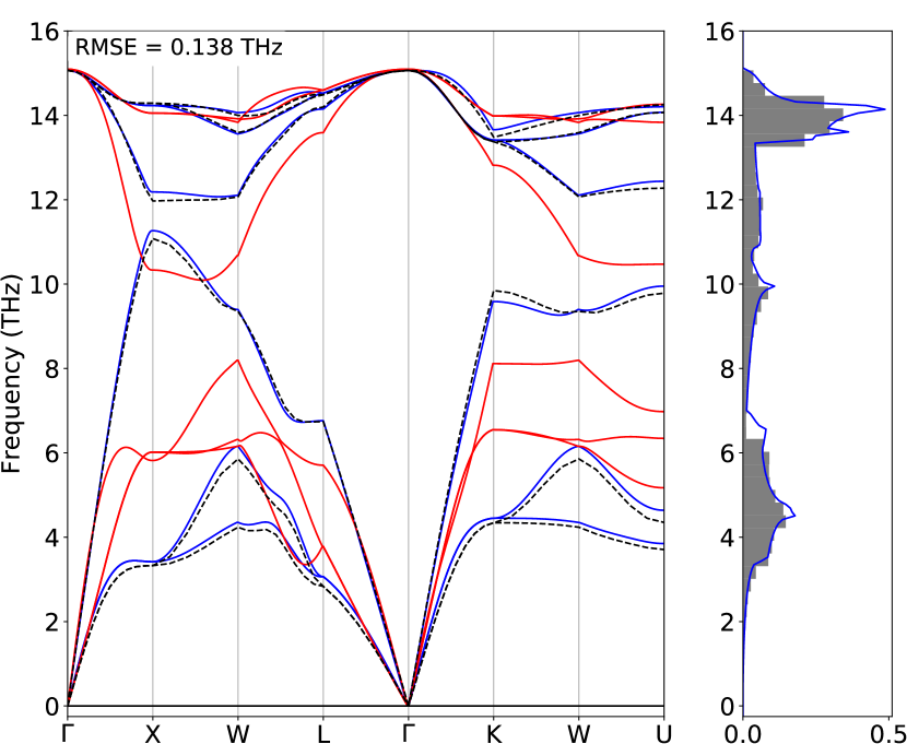
Figure 1: Phonon dispersion and density of states calculations by GAP trained using a minimal database only containing deformed primitive unit cells (red) and the full database containing NDSC configurations (blue). Reference DFT values are shown as black dashed lines.

We fitted a reduced model for Si that only contained the primitive unit cell configurations, in order to study the role of different elements of the database. Tabulated results in Table 3 show excellent agreement of elastic constants for both models. As the elastic moduli are related to the slope of the acoustic phonon modes near the $\Gamma$-pointBöer and Pohl (2018), portions of the dispersion of phonon modes are also in good agreement for the minimal model, as shown in Figure 1. However, at phonon modes corresponding to intermediate wavelengths the agreement for the minimal model is poor, confirming that deformed unit cells provide information to the GAP fitting about the elastic behaviour of a given material, but larger supercells are required to inform the fitting procedure on the full FCM. Indeed, adding NDSC configurations to the database, we recover the phonon dispersion across the BZ accurately.

Figure 2: GAP models trained using NDSC structures (blue) versus commensurate DFT (black dashed) phonon dispersion calculations for bcc W (top panel) and fcc Al (bottom panel) with corresponding density of states.

The GAP model reproduces the elastic and vibrational properties of bcc W to a great accuracy, although we note that the largest error compared to DFT in the phonon frequencies is at the $H$ point, together with a discrepancy in the curvature along the $P-H$ direction. Since the phonon mode at $H$ corresponds to displacing oppositely the two atoms located on neighbouring corners of the cubic cell, the corresponding elements of the FCM can be regarded as well represented in our database.

To illustrate the efficiency gains realised when using NDSC configurations in the training set, we compare the phonon dispersion curves corresponding to two GAP models, constructed to emphasise the advantage of using configurations consisting of fewer atoms. The two models were based on two separate databases, both of which required the same amount of computational time to calculate the ab initio reference energies, forces and virial stresses. To generate the first database, we used DSC of size commensurate with the desired q-point sampling, where only a single atom is displaced from its ideal lattice site, as suggested by George et alGeorge et al (2020). The other database contained NDSC configurations generated using the workflow described in Section III.2, such that the same amount of computational effort was needed to compute the ab initio data as for the diagonal supercell. The comparison of the phonon dispersion of the two models is presented in Figure 3.

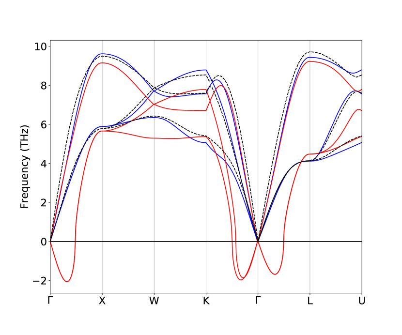
Figure 3: GAP for Al based on NDSC (blue line, 66.1 CPU hours) and diagonal supercell (red line, 60.1 CPU hours) data as compared against underlying DFT (black dashed line) for a minimal amount of data.

The model fitted on NDSC configurations performs noticeably better, with phonon modes in close agreement with the ab initio reference data. On the other hand, while the model fitted with diagonal supercells captures some of the phonon branches, it predicts unphysical dynamical instabilities in fcc Al.

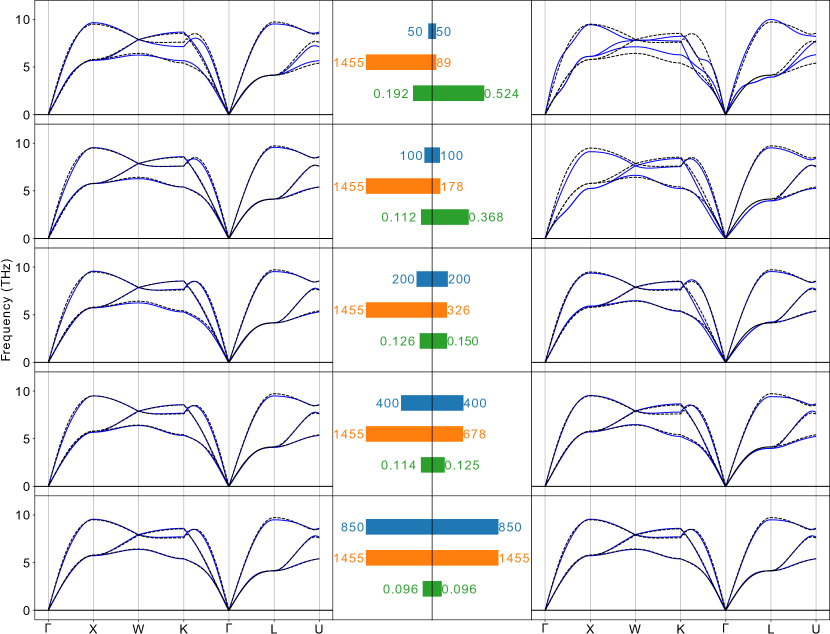
Figure 4: Left and right: Phonon dispersion curves of fcc Al GAP models (blue) compared to the DFT reference (black dashed). The set of training configurations increases from the top to the bottom, with the number of atomic environments displayed as blue bars (with numbers) on the centre panel. The orange bars represent the number of representative (sparse) points in each of the GAP models, and the green bars show the RMSE of the phonon frequencies in THz units.

To establish how the performance and accuracy of our MLIP models benefit from increasing the amount of training data, we fitted a series of GAP models for Al, using different size random subsets of the NDSC data. We present our learning curves as a series of phonon dispersion diagrams in Figure 4, showing two approaches: (a) keeping the set of representative atomic environments (or sparse points, set $M$ in equation 1) constant across the models, using the representative set selected from atomic environments in the largest data set; (b) selecting representative atomic environments from each of the fitting subset. As expected, increasing the data size leads to significant but diminishing improvements the accuracy of the model, measured as RMSE of the predicted phonon dispersion against the ab initio benchmark. However, it is interesting to observe that when the sparse points, which represent basis functions in the GAP framework, are selected from atomic environments not necessarily present in the training configurations, the accuracy is markedly improved even when using the same fitting targets. Therefore we suggest that GAP models may be improved by adding atomic configurations that do not need ab initio data associated with them, in order to increase the set of sparse points. The advantage of this approach is that significantly less computational effort is needed to generate the expensive ab initio data and it is possible to make improvements without the need to calculate additional target quantities at the DFT level.

We were also interested in studying how NDSC configurations may assist fitting the PES at stationary points other than minima. Aluminium at ambient conditions is dynamically unstable in the body-centred cubic form, although at extreme pressures the bcc phase becomes energetically favourable Sin’ko and Smirnov (2002). We have collected training configurations along the Bain path that connects the bcc and fcc phases of Al. The lattice vectors of primitive unit cells were described as body-centred tetragonal,

$$\mathbf{L}=\begin{bmatrix}-\nicefrac{{a}}{{2}}&\nicefrac{{a}}{{2}}&\nicefrac{{c}}{{2}}\\ \nicefrac{{a}}{{2}}&-\nicefrac{{a}}{{2}}&\nicefrac{{c}}{{2}}\\ \nicefrac{{a}}{{2}}&\nicefrac{{a}}{{2}}&-\nicefrac{{c}}{{2}}\\ \end{bmatrix}$$ (7)

where the rows of $\mathbf{L}$ represent the cell vectors, and $a$ and $c$ change as

$$a =a_{0}(1-\eta+2^{\nicefrac{{1}}{{3}}}\eta)$$

$$c =\frac{a_{0}}{\sqrt{1-\eta+2^{\nicefrac{{1}}{{3}}}\eta}}$$

with $0\leq\eta\leq 1$, such that the volume of the cell $|\det{\mathbf{L}}|$ is conserved. With this definition, the cases $\eta=0$ and $\eta=1$ correspond to the bcc and fcc lattices, respectively. We fitted a GAP model based on perturbed NDSC configurations that were generated using primitive unit cells at $\eta=0,\nicefrac{{1}}{{2}}\textrm{ and }1$. We benchmarked the phonon dispersion curves obtained with our model considering intermediate $\eta$ values, as shown in Figure 6. We found excellent agreement with DFT overall, with instabilities at the $N$-point reproduced highly accurately.

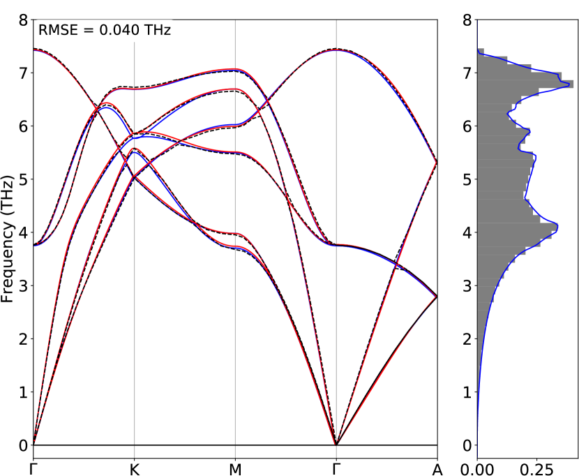
Figure 5: GAP trained using NDSC (blue) with component wise regularisation as informed by the force on each atom and virial stress on each configuration compared to a model where the regularisation is set to a constant value (red line) as well as DFT (black dashed) phonon dispersion curves.

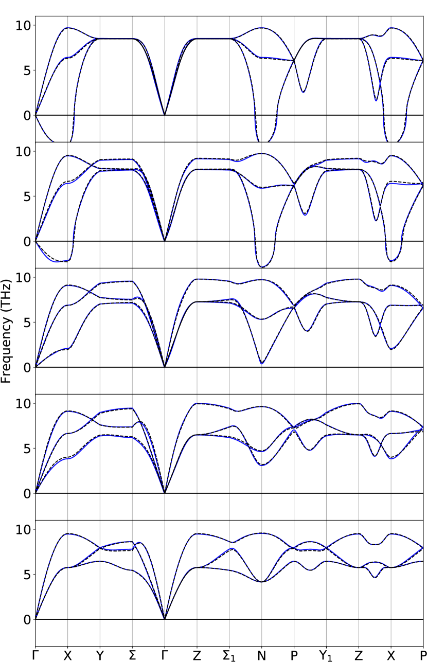
Figure 6: GAP (blue) trained using NDSC structures compared to commensurate DFT (black dashed) phonon dispersion calculations for in Al, where the lattice was transformed from the stable fcc structure (bottom) to the dynamically unstable bcc structure (top) along the Bain path.

We have also included a non-cubic crystalline system, magnesium, in our benchmarks, whose ground state structure at ambient condition is hexagonal close packed. Using NDSC configurations to train a GAP model, we find excellent agreement between the GAP and the ab initio phonon dispersion curves.

While accurate phonon spectra on acoustic modes near the $\Gamma$-point indicate that the elastic properties of the crystal are well representedBöer and Pohl (2018), it is insightful to directly examine the numerical values of the elastic constants of the MLIP models for additional benchmarking purposes. Table 3 and Figure 7 summarise the elastic moduli computed at the relaxed geometries both using DFT and the GAP models, showing excellent agreement with up to 6% error.

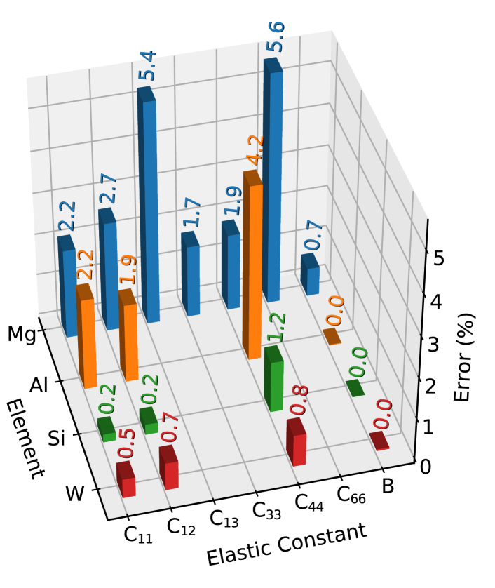
Figure 7: Relative error of elastic constants of GAP models of Mg (blue), Al (orange), Si (green) and W (red) compared to DFT results.

Figure 8: Errors of elastic constants of GAP models of Mg relative to DFT values in the hcp crystal structure. GAP models were fitted using static force and virial regularisation (orange bars and figures) and adaptive force and virial regularisation (blue bars and figures), as described in section III.3.

We illustrate the effect of adaptive regularisation of individual virial stress components, introduced in Section III.2, by comparing two Mg GAP models, one of which uses a static regularisation of 0.01 eV for each virial component, while the other employing the adaptive scheme. As shown in Figure 8, some of the elastic constants are only reproduced to an error of up to 7%, while introducing the adaptive virial regularisation, accuracy is significantly improved across all elastic constants without any deterioration of the quality of the phonon dispersion curves depicted in Figure 5.

V Conclusions

In conclusion, we explored a computationally efficient approach using the NDSC method introduced by Lloyd-Williams and Monserrat to generate database configurations for fitting MLIP models based on ab initio data. We found that NDSC configurations provide sufficient data to fit MLIP reproducing the FCM near stationary points of bulk crystalline materials, while costing significantly less computational effort than diagonal supercells. We have also suggested an adaptive scheme to regularise virial stress components of ab initio databases and demonstrated improvements of the elastic behaviour of MLIP. The procedure described in this work can be fully automated and integrated into existing database generating workflows, allowing to save computational cost or include a greater variety of representative structures, realising savings on cost and carbon emissions associated with high-performance computations, or improved quality MLIP. We also envisage further use of NDSC configurations in databases used to inform models for alloy materials, as an addition or alternative to semi quasi-random structures, where the substitution of elemental species may be regarded as alchemical perturbations.

VI Software and data availability

All ab initio training data and the scripts used to generate the configurations are made available in a dedicated repositoryrep . We used the QUIP software package with the GAP pluginqui , available under the General Public License and the Academic Source License, respectively. The Atomic Simulation EnvironmentLarsen et al. (2017) was used to manipulate atomic configurations and we employed the phonopy packageTogo and Tanaka (2015b) to calculate the phonon dispersion curves of the GAP models. Our workflow greatly benefited from using GNU parallelTange (2022).

VII Acknowledgments

We thank Noam Bernstein and Keith Refson for fruitful discussions. We acknowledge support from the NOMAD Centre of Excellence, funded by the European Commission under grant agreement 951786. CA is supported by a studentship jointly by the UK Engineering and Physical Sciences Research Council–supported Centre for Doctoral Training in Modelling of Heterogeneous Systems, Grant No. EP/S022848/1 and the Atomic Weapons Establishment. ABP acknowledges funding from CASTEP-USER funded by UK Research and Innovation under the grant agreement EP/W030438/1. Calculations were performed using the Sulis Tier 2 HPC platform hosted by the Scientific Computing Research Technology Platform at the University of Warwick. Sulis is funded by EPSRC Grant EP/T022108/1 and the HPC Midlands+ consortium. We acknowledge the University of Warwick Scientific Computing Research Technology Platform for assisting the research described within this study.