Training Stronger Spiking Neural Networks with Biomimetic Adaptive Internal Association Neurons

Abstract

As the third generation of neural networks, spiking neural networks (SNNs) are dedicated to exploring more insightful neural mechanisms to achieve near-biological intelligence. Intuitively, biomimetic mechanisms are crucial to understanding and improving SNNs. For example, the associative long-term potentiation (ALTP) phenomenon suggests that in addition to learning mechanisms between neurons, there are associative effects within neurons. However, most existing methods only focus on the former and lack exploration of the internal association effects. In this paper, we propose a novel Adaptive Internal Association (AIA) neuron model to establish previously ignored influences within neurons. Consistent with the ALTP phenomenon, the AIA neuron model is adaptive to input stimuli, and internal associative learning occurs only when both dendrites are stimulated at the same time. In addition, we employ weighted weights to measure internal associations and introduce intermediate caches to reduce the volatility of associations. Extensive experiments on prevailing neuromorphic datasets show that the proposed method can potentiate or depress the firing of spikes more specifically, resulting in better performance with fewer spikes. It is worth noting that without adding any parameters at inference, the AIA model achieves state-of-the-art performance on DVS-CIFAR10 (83.9%) and N-CARS (95.64%) datasets.

Index Terms—  Adaptive Internal Association Neuron, Spiking Neural Networks, Bionic Learning, Neuromorphic Data

1 Introduction

Inspired by the learning mechanisms of the mammalian brain, spiking neural networks (SNNs) are considered a promising model for artificial intelligence (AI) and theoretical neuroscience [1]. In theory, as the third generation of neural networks, SNNs are computationally more powerful than traditional artificial neural networks (ANNs) [2, 3].

Essentially, SNNs are dedicated to exploring more insightful neural mechanisms to achieve near-biological intelligence. The most representative ones are the leaky integrate-and-fire (LIF) model [4, 5] and spike-timing-dependent plasticity (STDP) rules [1]. The LIF neuron model is a trade-off between biomimicry and computability. It can reflect most properties of biological neurons, while the calculation is relatively simple. STDP is a temporally asymmetric form of Hebbian learning that arises from the close temporal correlation between the spikes of two neurons, presynaptic and postsynaptic [3]. Both of them inspire us to understand and improve SNNs from biological mechanisms.

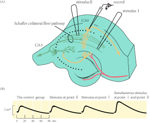
Fig. 1: The associative long-term potentiation phenomenon in hippocampal slices of rats. (A) Two different groups of Schaffer collateral presynaptic fibers (stimulation I and stimulation II) are stimulated while performing intracellular recording of CA1 (cornu Ammonis) pyramidal cells. (B) The average response of CA1 pyramidal cells to a stimulus from point II is observed. The curve depicts the membrane voltage change after point I and point II are stimulated separately and simultaneously for ten minutes under control conditions  [6].

The interesting associative long-term potentiation (ALTP) phenomenon [6] has recently attracted our attention, as shown in Fig. 1 (A). When points $I$ and $II$ were stimulated at the same time, the response of point $II$ was enhanced, but not when stimulated separately. The ALTP phenomenon suggests that in addition to learning mechanisms between neurons, there are associative effects within neurons.

However, most biologically inspired methods mainly focus on the learning between neurons and lack the exploration of associative effects within neurons. For example, spatiotemporal backpropagation based method [7] with surrogate gradient, time surfaces based method [8] to process the temporal information of SNNs, membrane potential based method [5] to rectify the distribution, membrane time constant based method [9] to avoid manual adjustment of neuron parameters, axonal delay based method [10] to simulate a short term memory, and other novel method [11, 4].

In this paper, we propose an adaptive internal associative (AIA) neuron model to establish neglected associations within neurons. Consistent with the ALTP phenomenon, the AIA neuron model is adaptive to input stimuli, and internal associative learning occurs only when both dendrites are stimulated simultaneously. Furthermore, we measure the strength of internal associations by weighting gradients passed between neurons with input weights. Therefore, the effect is positively correlated with input weights, as described in Eq 7. In addition, we introduce intermediate caching to reduce the volatility of associations. Extensive experiments demonstrate that the AIA neuron model can potentiate or depress the firing of spikes more specifically. This biomimetic model performs better with fewer spikes, which is closer to the efficiency of the brain. It is worth noting that without adding any parameters at inference, the AIA model achieves state-of-the-art performance on DVS-CIFAR10 (83.9%) and N-CARS (95.64%) datasets.

The closest works to the AIA model are the learning rules of Hebbian and STDP [1]. However, they both only focus on the learning mechanism between neurons, while AIA establishes the associations inside neurons.

2 Method

2.1 LIF Neuron Model

For spiking neurons, the neuronic membrane potential increases with the accumulation of weighted spikes, and an output spike is generated once the membrane potential exceeds a threshold. The membrane potential of widely used LIF model [4] is formulated as:

$$\tau_{m}\frac{du}{dt}=-\left(u-V_{rest}\right)+R_{m}\cdot I(t),\quad u<V_{th}$$ (1)

$$\left.\begin{aligned} u=V_{rest}&\\ o=\delta(t-t_{i})&\end{aligned}\right\},\quad u\geq V_{th}$$

where $\tau_{m}=R_{m}C_{m}$ is the membrane time constant, $R_{m}$ and $C_{m}$ are resistance constant and capacitance constant, respectively. $u$ is the membrane potential, $I(t)$ is the input current, $V_{th}$ and $V_{rest}$ are the spiking threshold and resting potential. Once $u$ reaches $V_{th}$ at $t_{i}$, a spike is generated and $u$ is reset to $V_{rest}$, which is usually taken as 0. The output spike $o$ is described by the Dirac delta function $\delta(x)$. The input will be summed to $I(t)$ by the dendrite response weight $w$. By absorbing the $1-dt/\tau_{m}$ and $1/C_{m}$ constants into response weights $w$ and leakage coefficient $\lambda$ respectively [7], the discrete form of Eq. 1 is described as:

$$u_{i}^{n+1,t+1}= \lambda u_{i}^{n+1,t}(1-o_{i}^{n+1,t})+x_{i}^{n+1,t+1}$$ (2)

$$x_{i}^{n+1,t+1}= \sum_{j}w_{ij}^{n+1}o_{j}^{n,t+1}$$

$$o_{i}^{n+1,t+1}= H(u_{i}^{n+1,t+1}-V_{th})$$

where n denotes the $n$-th layer and $w_{ij}$ is the synaptic weight from the $j$-th neuron in pre-layer $n$ to the $i$-th neuron in the post-layer $n+1$. $x_{i}$ denotes the weighted input, and $H(x)$ is the Heaviside step function, whose gradient is given by the surrogate method [7].

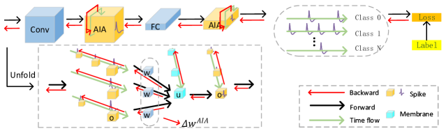
Fig. 2: The network Framework. Data and gradients flow along space and time, and $\Delta w^{AIA}$ is determined by the input weights.

2.2 Adaptive Internal Association Neuron Model

Motivation

The phenomenon of associative long-term potentiation [6] in Fig. 1 and the associated long-term depressive phenomenon [12] illustrates that there is an associative effect within neurons when stimulated at the same time. And the effect is positively correlated with input weights. These observations inspire us to explore the corresponding associative learning mechanisms within neurons.

AIA Neuron Model

As shown in Fig. 1, between different input synapses within a single neuron, associative learning occurs only when both input synapses are stimulated. Since the biological mechanism of the ALTP phenomenon is unclear, we hypothesized that a function $f(x)$ acting on dendrites could establish stimulus-adaptive associative learning. We will discuss the form of this function in Sec. 2.3. Adding the associative learning term $f(x)$ to Eq. 2, the adaptive internal associative (AIA) neuron model can be formulated as:

$$u_{i}^{n+1,t+1}= \lambda u_{i}^{n+1,t}(1-o_{i}^{n+1,t})+f(x_{i}^{n+1,t+1})$$ (3)

$$x_{i}^{n+1,t+1}= \sum_{j}w_{ij}^{n+1}o_{j}^{n,t+1}$$

$$o_{i}^{n+1,t+1}= H(u_{i}^{n+1,t+1}-V_{th})$$

2.3 Derivation of Gradients

For the LIF model, the gradient of the weights is given by:

$$\Delta w_{ij}^{LIF} =\frac{\partial L}{\partial w_{ij}^{n+1}}=\frac{\partial L}{\partial u_{i}^{n+1,t+1}}\frac{\partial u_{i}^{n+1,t+1}}{\partial x_{i}^{n+1,t+1}}\frac{\partial x_{i}^{n+1,t+1}}{\partial w_{ij}^{n+1}}$$ (4)

$$=\frac{\partial L}{\partial u_{i}^{n+1,t+1}}o_{j}^{n,t+1}$$

where L is the loss function. For the AIA neuron model, the gradient of the weights is given by:

$$\Delta w_{ij}^{AIA}=\frac{\partial L}{\partial w_{ij}^{n+1}} =\frac{\partial f(x_{i}^{n+1,t+1})}{\partial x_{i}^{n+1,t+1}}\frac{\partial L}{\partial u_{i}^{n+1,t+1}}o_{j}^{n,t+1}$$ (5)

Combining the observations in motivation, we can set the function $f^{\prime}(x)=x$ to construct a stimulus-adaptive internal associative neuron model. The $\Delta w_{ij}^{AIA}$ is formulated as:

$$\Delta w_{ij}^{AIA} =\left(\sum_{k}w_{ik}^{n+1}o_{k}^{n,t+1}\right)\frac{\partial L}{\partial u_{i}^{n+1,t+1}}o_{j}^{n,t+1}$$ (6)

where $k$ represents the neuron connected to neuron $i$. Note that $o\in\{0,1\}$, Eq. 6 can be expressed as:

$$\Delta w_{ij}^{AIA} =o_{j}^{n,t+1}*\sum_{k}o_{k}^{n,t+1}w_{ik}^{n+1}\Delta w_{ik}^{LIF}$$ (7)

When the neuron $j$ is in the resting state($o_{j}=0$), the weight $w_{ij}$ remains unchanged. When neuron $j$ inputs a stimulus ($o_{j}=1$), all neurons that simultaneously input a stimulus ($o_{k}=1$) affect $w_{ij}$. In other words, only when neuron $i$ is stimulated by both the $j$-th and $k$-th neurons will the corresponding associative effects be established within the neuron.

In addition, Eq. 7 measures the association influence with minimum cost by multiplexing the weights and the gradients between neurons. It turns out that the greater the synaptic response to the stimulus, the stronger the effect of associative learning, which is also consistent with the observations. Fig. 2 shows the network framework, and Eq. 3 and Eq. 7 represent computations in the forward and backward respectively.

2.4 Intermediate Cache

In practice, the gradient swings between $0$ and $w_{ik}^{n+1}\Delta w_{ik}^{LIF}$, which may cause the problem of “dead neurons”, so we introduce an intermediate cache variable $\beta$. Specifically, let $f^{\prime}(x)=\beta$, the gradients of $\Delta w_{ij}^{AIA}$ and $\beta$ are:

$$\Delta w_{ij}^{AIA}=\frac{\partial L}{\partial w_{ij}^{n+1}}=o_{j}^{n,t+1}*\beta\Delta w_{ij}^{LIF}$$ (8)

$$\frac{\partial L}{\partial\beta}=\sum_{k}o_{k}^{n,t+1}w_{ik}^{n+1}\Delta w_{ik}^{LIF}$$ (9)

It can be seen that, after adding the intermediate cache, $\beta$ accumulates gradients in Eq. 7 overall stimulated synapses and applies this association effect only to stimulated synapses. It is worth noting that the intermediate cache $\beta$, as an auxiliary tool for saving gradients, can be merged into $w$ for calculation at inference time, so it will not bring additional parameters.

Table 1: Performance of AIA neuron model and the SOTAs on CIFAR10-DVS, N-Caltech101 and N-CARS datasets.

Network	Method	Reference	Model	CIFAR10-DVS	N-Caltech101	N-CARS
CNNs-based	RG-CNNs [13]	TIP 2020	Graph-CNN	54.00	61.70	91.40
	SlideGCN [14]	ICCV 2021	Graph-CNN	68.00	76.10	93.10
	ECSNet [15]	T-CSVT 2022	LEE$\rightarrow$MA	72.70	69.30	94.60
SNNs-based	HATS[8]	CVPR 2018	HATS-SVM	52.40	64.20	81.0
	Dart[16]	TPAMI 2020	SPM-SVM	65.80	66.80	-
	STBP [7]	AAAI 2021	Resnet-19	67.80	-	-
	PLIF [9]	ICCV 2021	7-layer	74.80	-	-
	Dspike [17]	NeurIPS 2021	ResNet-18	75.40	-	-
	AutoSNN [18]	ICML 2022	-	72.50	-	-
	RecDis [5]	CVPR 2022	Resnet-19	72.42	-	-
	DSR [4]	CVPR 2022	VGG-11	77.27	-	-
	NDA [19]	ECCV 2022	VGG-11	81.70	78.20	90.1
	AIA	-	VGG-9	83.90	80.07	95.64

3 Experiments

Extensive experiments are conducted to demonstrate the superiority of the AIA neuron model. For a fair comparison, a LIF neuron model with the same parameters is used as the baseline. Specifically, the weights are initialized by kaiming distribution. The threshold and leakage coefficients $\lambda$ of neurons are 1 and 0.5 respectively. Adam optimizer is introduced to adjust the learning rate, which is initially set to $1\times 10^{-3}$.

3.1 Comparison with the State-of-the-Art

As shown in Tab. 1, we surpass previous state-of-the-art methods on DVS-CIFAR10 [20], N-Caltech101 [21], N-CARS [8] neuromorphic datasets. DVS-CIFAR10 contains 10,000 samples, carrying noise and blur caused by event cameras. We resize the samples to $64\times 64$ and achieve 83.9% accuracy. It is worth noting that NDA is the best performer in the previous work, but its sample size is $128\times 128$. To the best of our knowledge, the AIA neuron model achieves state-of-the-art performance on DVS-CIFAR10 dataset among all SNNs. N-Caltech101 is a spiking version of the original frame-based Caltech101 dataset. N-CARS is a large real-world event-based car classification dataset extracted from various driving courses. On these two datasets, we resize the samples to $48\times 48$, reaching the accuracy of 80.07% and 95.64% respectively. In conclusion, the AIA model achieves leading performance by establishing associations within neurons, which in turn illustrates the effectiveness of biomimetic internal associations.

3.2 Analysis of AIA Neuron Model

Table 2: The performance of different neuron models on N-Caltech101 datasets and CIFAR10-DVS datasets.

Neurons	N-Caltech101(%)	CIFAR10-DVS(%)
LIF	78.13	82.5
IF	75.94	81.9
PLIF	75.58	79.0
AIA	79.59	83.5
Cached AIA	80.07	83.9

Compared with other neuron models

Ablation experiments are performed on CIFAR10-DVS and N-Caltech101 datasets to further compare the effects of AIA and other neuronal models. We employ a publicly available implementation of PLIF neurons [9], which sets the membrane time constant as a trainable variable. As shown in Tab. 2, the AIA neuron model achieves the accuracy of 79.59% and 83.5%, surpassing the most commonly used neuron models under the same parameters. In addition, the intermediate cache also improves the AIA model (Cached AIA).

Insightful variations of the AIA model

To gain further insight into the workings of AIA neurons, we perform some analysis on the N-Caltech101 dataset. As shown in Fig. 3 (a), we calculate the weight distribution of the AIA model and the LIF model respectively, and obtain the normalized changes in different intervals. Red indicates that the number of weights in the interval is increasing, and blue indicates that it is decreasing. It turns out that the weights escape from intervals close to 0, implying a larger change in membrane voltage. In other words, AIA neurons can more effectively potentiate or depress the firing of spikes, resulting in better extraction of key features.

In addition, the change in the number of spikes is shown in Fig. 3 (b). The AIA model significantly affects the number of fired spikes, especially in feature extraction layers. Notably, the number of fired spikes is significantly reduced overall, implying that the AIA neuron model performs better with fewer spikes. It indicates that the biomimetic internal association mechanism inherently improves the efficiency and biological plausibility of the model.

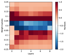
(a) Weight distribution.

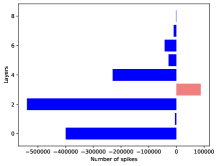
(b) Number of spikes.

Fig. 3: Variations in weight distribution and number of spikes after using AIA neurons compared to LIF neurons.

4 Conclusion

Inspired by the ALTP phenomenon, we propose a novel adaptive internal association (AIA) neuron model. This biomimetic model achieves state-of-the-art performance on neuromorphic datasets. In addition, the intermediate cache is introduced to reduce volatility. The insightful analysis shows that AIA neurons can more effectively potentiate or depress the firing of spikes and perform better with fewer spikes. And the proposed neuron model can provide the basis for more efficient and biologically plausible spiking neural networks.

References

- [1] Kaushik Roy, Akhilesh Jaiswal, and Priyadarshini Panda, “Towards spike-based machine intelligence with neuromorphic computing,” Nature, vol. 575, 2019.
- [2] Wolfgang Maass, “Networks of spiking neurons: The third generation of neural network models,” Neural Networks, vol. 10, no. 9, pp. 1659–1671, 1997.
- [3] Duzhen Zhang, Tielin Zhang, Shuncheng Jia, Qingyu Wang, and Bo Xu, “Recent advances and new frontiers in spiking neural networks,” in Proceedings of the Thirty-First International Joint Conference on Artificial Intelligence, IJCAI 2022, Vienna, Austria, 23-29 July 2022, Luc De Raedt, Ed. 2022, pp. 5670–5677, ijcai.org.
- [4] Qingyan Meng, Mingqing Xiao, Shen Yan, Yisen Wang, Zhouchen Lin, and Zhi-Quan Luo, “Training high-performance low-latency spiking neural networks by differentiation on spike representation,” in Proceedings of the IEEE/CVF Conference on Computer Vision and Pattern Recognition, 2022, pp. 12444–12453.
- [5] Yufei Guo, Xinyi Tong, Yuanpei Chen, Liwen Zhang, Xiaode Liu, Zhe Ma, and Xuhui Huang, “Recdis-snn: Rectifying membrane potential distribution for directly training spiking neural networks,” in CVPR, 2022, pp. 326–335.
- [6] G Barrionuevo and T H Brown, “Associative long-term potentiation in hippocampal slices,” Proceedings of the National Academy of Sciences, vol. 80, no. 23, pp. 7347–7351, 1983.
- [7] Hanle Zheng, Yujie Wu, Lei Deng, Yifan Hu, and Guoqi Li, “Going deeper with directly-trained larger spiking neural networks,” in Proceedings of the AAAI Conference on Artificial Intelligence, 2021, pp. 11062–11070.
- [8] Amos Sironi, Manuele Brambilla, Nicolas Bourdis, Xavier Lagorce, and Ryad Benosman, “Hats: Histograms of averaged time surfaces for robust event-based object classification,” in CVPR, June 2018.
- [9] Wei Fang, Zhaofei Yu, Yanqi Chen, Timothée Masquelier, Tiejun Huang, and Yonghong Tian, “Incorporating learnable membrane time constant to enhance learning of spiking neural networks,” in ICCV, 2021, pp. 2661–2671.
- [10] Pengfei Sun, Longwei Zhu, and Dick Botteldooren, “Axonal delay as a short-term memory for feed forward deep spiking neural networks,” in IEEE International Conference on Acoustics, Speech and Signal Processing, ICASSP 2022, Virtual and Singapore, 23-27 May 2022. 2022, pp. 8932–8936, IEEE.
- [11] Tielin Zhang, Yi Zeng, Dongcheng Zhao, and Bo Xu, “Brain-inspired balanced tuning for spiking neural networks,” in IJCAI, 7 2018, pp. 1653–1659.
- [12] Patric K. Stanton and Terrence J. Sejnowski, “Associative long-term depression in the hippocampus induced by hebbian covariance,” Nature, vol. 339, 1989.
- [13] Yin Bi, Aaron Chadha, Alhabib Abbas, Eirina Bourtsoulatze, and Yiannis Andreopoulos, “Graph-based spatio-temporal feature learning for neuromorphic vision sensing,” IEEE Trans. Image Process., vol. 29, pp. 9084–9098, 2020.
- [14] Yijin Li, Han Zhou, Bangbang Yang, Ye Zhang, Zhaopeng Cui, Hujun Bao, and Guofeng Zhang, “Graph-based asynchronous event processing for rapid object recognition,” in 2021 IEEE/CVF International Conference on Computer Vision, ICCV 2021, Montreal, QC, Canada, October 10-17, 2021. 2021, pp. 914–923, IEEE.
- [15] Zhiwen Chen, Jinjian Wu, Junhui Hou, Leida Li, Weisheng Dong, and Guangming Shi, “Ecsnet: Spatio-temporal feature learning for event camera,” IEEE Transactions on Circuits and Systems for Video Technology, pp. 1–1, 2022.
- [16] Bharath Ramesh, Hong Yang, Garrick Orchard, and et al., “Dart: Distribution aware retinal transform for event-based cameras,” TPAMI, vol. 42, no. 11, pp. 2767–2780, 2020.
- [17] Yuhang Li, Yufei Guo, Shanghang Zhang, Shikuang Deng, Yongqing Hai, and Shi Gu, “Differentiable spike: Rethinking gradient-descent for training spiking neural networks,” Advances in Neural Information Processing Systems, vol. 34, pp. 23426–23439, 2021.
- [18] Byunggook Na, Jisoo Mok, Seongsik Park, Dongjin Lee, Hyeokjun Choe, and Sungroh Yoon, “Autosnn: Towards energy-efficient spiking neural networks,” arXiv preprint arXiv:2201.12738, 2022.
- [19] Yuhang Li, Youngeun Kim, Hyoungseob Park, Tamar Geller, and Priyadarshini Panda, “Neuromorphic data augmentation for training spiking neural networks,” arXiv preprint arXiv:2203.06145, 2022.
- [20] Hongmin Li, Hanchao Liu, Xiangyang Ji, and et al., “Cifar10-dvs: An event-stream dataset for object classification,” Frontiers in Neuroscience, vol. 11, pp. 309, 2017.
- [21] Garrick Orchard, Ajinkya Jayawant, Gregory Cohen, and Nitish V. Thakor, “Converting static image datasets to spiking neuromorphic datasets using saccades,” CoRR, vol. abs/1507.07629, 2015.