Distributed Robust Principal Component Analysis

Abstract

We study the robust principal component analysis (RPCA) problem in a distributed setting. The goal of RPCA is to find an underlying low-rank estimation for a raw data matrix when the data matrix is subject to the corruption of gross sparse errors. Previous studies have developed RPCA algorithms that provide stable solutions with fast convergence. However, these algorithms are typically hard to scale and cannot be implemented distributedly, due to the use of either SVD or large matrix multiplication. In this paper, we propose the first distributed robust principal analysis algorithm based on consensus factorization, dubbed DCF-PCA. We prove the convergence of DCF-PCA and evaluate DCF-PCA on various problem settings.

1 Introduction

Principal robust analysis (PCA) has been widely used for dimension reduction in data science. It extracts the top $k$ significant components of a given matrix by computing the best low-rank approximation. However, it is well known that PCA is sensitive to noises and adversarial attacks. Robust PCA (RPCA) aims at mitigating this drawback by separating the noise out explicitly. Specifically, RPCA assumes that the observed matrix $M\in\mathbb{R}^{m\times n}$ can be decomposed as $M=L^{*}+S^{*}$ where $L^{*}$ is a low-rank matrix and $S^{*}$ is a sparse matrix. The goal of RPCA is to recover the low-rank matrix $L^{*}$ from the noisy data $M$, which is typically expressed as an optimization problem:

$$\min_{L,S}\mathbf{rank}(L)+\lambda\|S\|_{0},\ \mathrm{s.t.}\ M=L+S.$$ (1)

Unfortunately, this optimization problem is known to be NP-hard. Therefore, Equation 1 is often reformulated to other optimization problems listed below.

• Convex relaxation of $\mathbf{rank}(\cdot)$ to nuclear norm $\|\cdot\|_{*}$ and $\ell_{0}$ norm to $\ell_{1}$ norm.

  $$\min_{L,S}\|L\|_{*}+\lambda\|S\|_{1},\ \mathrm{s.t.}\ M=L+S.$$ (2)

  where the nuclear norm is defined as sum of singular values $\|L\|_{*}=\sum_{i=1}^{\min(m,n)}\sigma_{i}(L)$ and $\|S\|_{1}$ denotes the $\ell_{1}$ norm of $S$ as a vector: $\|S\|_{1}=\sum_{ij}|S_{ij}|$.

• A variant of RPCA considers recovering $L$ from another noise with bounded Frobenius norm. The corresponding optimization problem is formulated as

  $$\min_{L,S}\|L\|_{*}+\lambda\|S\|_{1}+\frac{\mu}{2}\|L+S-M\|_{F}^{2}.$$ (3)

• Other works attempt to solve RPCA based on the low-rank matrix factorization that decomposes a low-rank matrix $M$ as $M=UV^{T}$ ($U\in\mathbb{R}^{m\times r},V\in\mathbb{R}^{n\times r}$). The rank function is resolved by an implicit constraint that $\mathbf{rank}(UV^{T})\leq r$. Feng el al. [1] proposed to optimize a nonconvex problem:

  $$\min_{U,V,S}\frac{1}{2}\|UV^{T}+S-M\|^{2}_{F}+\frac{\rho}{2}(\|U\|^{2}_{F}+\|V\|^{2}_{F})+\lambda\|S\|_{1}$$ (4)

  which exploited the property of nuclear norm [2] so that its global minimum also minimizes the objective of Equation 3:

  $$\|L\|_{*}=\inf_{U,V}\left\{\frac{1}{2}\|U\|_{F}^{2}+\frac{1}{2}\|V\|_{F}^{2}:UV^{T}=L\right\}$$ (5)

The convex problems Equations 2 and 3 are well-posed and can be optimized using standard convex optimization methods, e.g., SDP, PGM and ADMM. However, the existence of the nuclear norm $\|\cdot\|_{*}$ makes it difficult for these algorithms to scale, since it cannot be calculated distributively.

In this paper, we present a distributed RPCA algorithm based on consensus factorization (DCF-PCA), which solves the nonconvex problem Equation 4 distributedly. We formalize the distributed RPCA problem and elaborate our DCF-PCA algorithm in Section 2; provides theoretical guarantees for DCF-PCA in Section 3; and exhibits numerical results for DCF-PCA in Section 4.

2 Distributed Robust Principal Component Analysis

2.1 Problem Definition

We formalize the problem of distributed robustness principal component problem. Assume the data $M\in\mathbb{R}^{m\times n}$ are distributed over $E$ remote clients. Each client $i\in[E]$ only has access to some columns of the matrix $M$.

$$M=\begin{bmatrix}M_{1}&M_{2}&\dots&M_{E}\end{bmatrix},\ \text{where}\ M_{i}\in\mathbb{R}^{m\times n_{i}}\ \text{and}\ n=\sum_{i=1}^{E}n_{i}.$$ (6)

For clarity, we define $L_{i}^{*}$ and $S_{i}^{*}$ such that $M_{i}=L_{i}^{*}+S_{i}^{*}$ for all $i\in[E]$.

Limited Communication. As the communication cost over remote devices are typically high, we give limited communication budget for the clients. Assuming $m=O(n)$, naively broadcasting the whole matrix needs transmitting a prohibitively large amount of data $O(n^{2}K)$.

Privacy Preserving. Privacy is considered as one of the most crucial issues in distributed learning. In practice, some local data $M_{i}$ may be privacy-sensitive and cannot be exposed to other clients. We call a distributed scheme privacy-preserving for a set of sensitive clients $\mathcal{I}$, if it recovers $L_{i}$ for $i\not\in\mathcal{I}$ but protects $M_{i}$ for $i\in\mathcal{I}$.

2.2 Distributed RPCA algorithm via consensus factorization

Algorithm 1 Distributed RPCA algorithm via consensus factorization (DCF-PCA)

Input: $E$ remote clients with submatrices $\{M_{1},\dots,M_{E}\}$.

Initialize matrix $U^{(0)}\in\mathbb{R}^{m\times r}$. Each client $i\in[E]$ randomly initializes $V_{i}\in\mathbb{R}^{n_{i}\times r},S_{i}\in\mathbb{R}^{m\times n_{i}}.$

for $t=0$ to $T-1$ do

     Server broadcasts $U^{(t)}$ to all clients.

     for each client $i\in[E]$ (concurrently) do

         Set $U_{i}^{(0)}$ as $U^{(t)}$ and $V_{i}^{(0)},S_{i}^{(0)}$ as $V_{i}^{(K)},S_{i}^{(K)}$ from the last epoch.

         for $k=0$ to $K-1$ do

$$(V_{i}^{(k+1)},S_{i}^{(k+1)})\leftarrow\arg\min_{V,S}\frac{1}{2}\|U^{(k)}V^{T}+S-M_{i}\|^{2}_{F}+\frac{\rho}{2}\|V\|_{F}^{2}+\lambda\|S\|_{1}$$ (7)

$$U_{i}^{(k+1)}\leftarrow U^{(k)}-\eta\nabla_{U}\mathcal{L}_{i}(U^{(k)},V_{i}^{(K)},S_{i}^{(k)})$$ (8)

         end for

         Send back the updated $U_{i}^{(t)}=U_{i}^{(K)}$ to the server

     end for

     Server aggregates all $U_{i}$ by average:

$$U^{(t+1)}\leftarrow\frac{\sum_{i=1}^{E}U_{i}^{(t)}}{E}$$ (9)

end for

$L_{i}=U^{(T)}{V_{i}^{(K)}}^{T}$ and $S_{i}=S_{i}^{(K)}$

return Recovered matrices $\{(L_{i},S_{i})\}_{i\in\mathcal{I}_{\text{public}}}$

Here, we present a distributed consensus-factorization based RPCA algorithm DCF-PCA to solve the problem defined in Section 2.1. We summarize our DCF-PCA algorithm in Algorithm 1. This algorithm uses the nonconvex objective function Equation 4 to avoid using nuclear norm. We claim that this objective function is perfectly separable for each client, making it suitable for the distributed optimization.

We define local objective functions for each $i\in[E]$:

$$\tilde{\mathcal{L}_{i}}(U_{i},V_{i},S_{i})=\frac{1}{2}\|U_{i}V_{i}^{T}+S_{i}-M_{i}\|_{F}^{2}+\frac{\rho}{2}\|V_{i}\|_{F}^{2}+\lambda\|S_{i}\|_{1}.$$ (10)

The overall optimization goal Equation 4 can be written as a summation over each client: $\mathcal{L}(U,V,S)=\sum_{i=1}^{E}\tilde{\mathcal{L}_{i}}(U_{i},V_{i},S_{i})+\frac{\rho}{2}\|U\|_{F}^{2}$. As a result, Equation 4 can be decomposed into multiple subproblems for each client to solve.

In order to enforce $\mathbf{rank}([L_{1}\ L_{2}\ \dots\ L_{E}])\leq r$, we require each client to reach a consensus on their left matrix $U_{i}$, i.e., every matrix $U_{i}$ must be identical. Therefore, we absorb the $\frac{\rho}{2}\|U\|_{F}^{2}$ term into each $\tilde{\mathcal{L}_{i}}(U_{i},V_{i},S_{i})$, so the local objective under consensus is

$$\mathcal{L}_{i}(U,V_{i},S_{i})=\tilde{\mathcal{L}_{i}}(U,V_{i},S_{i})+\frac{n_{i}\rho}{2n}\|U\|_{F}^{2}.$$ (11)

The problem can thus be reformulated into finding a solution for

$$U^{*}\in\arg\min_{U}g(U)=\arg\min_{U}\sum_{i=1}^{E}g_{i}(U)$$ (12)

where

$$g_{i}(U) =\inf_{V_{i},S_{i}}\mathcal{L}_{i}(U,V_{i},S_{i})$$

$$=\inf_{V_{i},S_{i}}\left(\frac{1}{2}\|UV_{i}^{T}+S_{i}-M_{i}\|_{F}^{2}+\frac{\rho}{2}(\|V_{i}\|_{F}^{2}+\frac{n_{i}}{n}\|U\|_{F}^{2})+\lambda\|S_{i}\|_{1}\right)$$ (13)

Equation 7 is a minimization problem of a convex function and the details of solving it is explained later. Equation 8 updates the matrix $U$ locally based on the surrogate optimal solution $(V_{i}^{*},S_{i}^{*})$. As we will see in (Section 3.2 (Lemma 2), Equation 8 executes one step of local gradient descent for $U$ optimizing the local objective $g_{i}(U)$, when the solution $(V_{i}^{*},S_{i}^{*})$ is exact.

Finally, Equation 9 aggregates the outputs from remote clients by average. This scheme is known as the FedAvg [3] algorithm in federated learning. When $K=1$, Equation 9 is equivalent to performing exactly one step of the global gradient descent following Equation 12. However, in practise, the communication cost among remote clients is non-negligible. Setting $K>1$ allows clients to run local gradient descent for multiple steps, reducing the communication overheads caused by synchronization. Moreover, it has been shown that choosing either a diminishing learning rate or a carefully designed fixed learning rate $\eta=O(\frac{1}{\sqrt{KT}})$ guarantees the convergence of FedAvg algorithm [4, 5].

Details of solving Equation 7. Here we elaborate the details for optimizing the convex function Equation 7. We claim that the solution for the convex local optimization problem

$$\{V_{i}^{*},S_{i}^{*}\}=\arg\min_{V_{i},S_{i}}\frac{1}{2}\|UV_{i}^{T}+S_{i}-M_{i}\|^{2}_{F}+\frac{\rho}{2}\|V_{i}\|^{2}_{F}+\lambda\|S_{i}\|_{1}$$ (14)

is unique. This is because $(V_{i},S_{i})$ is the solution for Equation 14 only if

$$(U_{i}^{T}U_{i}+\rho I)V^{T}V=U_{i}^{T}(M_{i}-S_{i})V_{i}$$ (15)

$$S_{i}=\mathrm{sign}(M_{i}-U_{i}V_{i}^{T})\cdot\max(|M_{i}-U_{i}V_{i}^{T}|-\lambda,0)$$ (16)

Bringing Equation 16 back to Equation 14 yields:

$$V_{i}^{*} \in\arg\min_{V_{i}\in\mathbb{R}^{n_{i}\times r}}\left[\frac{\rho}{2}\|V_{i}\|_{F}^{2}+\min_{S_{i}\in\mathbb{R}^{m\times n_{i}}}\left(\frac{1}{2}\|UV_{i}^{T}+S_{i}-M_{i}\|_{F}^{2}+\lambda\|S_{i}\|_{1}\right)\right]$$

$$=\arg\min_{V_{i}\in\mathbb{R}^{n_{i}\times r}}\left(\frac{\rho}{2}\|V_{i}\|_{F}^{2}+H_{\lambda}(M_{i}-UV_{i}^{T})\right).$$ (17)

where $H_{\lambda}(\cdot)$ is the Huber loss, as defined in Appendix A. We denote the inner objective by $h(V_{i})=\frac{\rho}{2}\|V_{i}\|_{F}^{2}+H_{\lambda}(M_{i}-UV_{i}^{T})$. We show by Lemma 1 in Section 3.2 that $h(V_{i})$ is $\rho$-strongly convex, which means the solution for Equation 17 is unique. Moreover, Lemma 1 guarantees a linear convergence for applying gradient descent on $V_{i}$ to optimize $h(V_{i})$. As a result, the convex problem in Equation 7 can be solved efficiently.

Problems with Unknown Exact Rank Attentive readers may notice that factorization-based algorithms including our Algorithm 1 require knowing the exact rank $r$ of the underlying low-rank matrix $L_{0}$. A more general problem formulation [6] considers anticipating an upper bound for the rank of $L_{0}$, i.e., $\mathbf{rank}(L_{0})\leq p$.

To solve this harder problem, DCF-PCA is slightly modified such that $U\in\mathbb{R}^{m\times p}$ and $V_{i}\in\mathbb{R}^{n_{i}\times p}$. As long as the incoherence condition [7] (as explained detailedly in Appendix A) is satisfied, the global minimizer of Equation 4 is still guaranteed to be the exact recovery, because of the property of nuclear norm: $\|L\|_{*}=\inf_{U,V}\frac{1}{2}\{\|U\|_{F}^{2}+\|V\|_{F}^{2}:UV^{T}=L\}$. We also confirm this statement numerically in Section 4.

Privacy Preserving. We claim that DCF-PCA also works for privacy critical scenarios. It learns a left matrix $U$ on consensus over all clients, but the private right matrices $V_{i}$ are kept secret for individuals. As suggested in Algorithm 1, DCF-PCA reveals $L_{i}$ only for public data $i\in\mathcal{I}_{\text{public}}$ and keeps $M_{i}$ secret for $i\in\mathcal{I}_{\text{private}}$.

3 Theoretical Analysis

3.1 Preliminaries

We first define some terminologies before going to details of the convergence analyses.

Definition 1 (Smoothness).

Consider a $C^{1}$-continuous function $f:\mathbb{R}^{d}\to\mathbb{R}$. We call the function $L$-smooth if its derivative is $L$-Lipschitz, i.e.,

$$\|\nabla f(w_{1})-\nabla f(w_{2})\|_{2}\leq L\|w_{1}-w_{2}\|_{2}.$$ (18)

Definition 2 (Strongly convex).

We call a $C^{1}$-continuous function $f:\mathbb{R}^{d}\to\mathbb{R}$ $\mu$-strongly convex, if $f(w)-\frac{\mu}{2}\|w\|_{2}^{2}$ is a convex function.

3.2 Convergence Analysis

In this section, we analyze the convergence rate of our distributed RPCA algorithm. The optimization variables are assumed to be bounded during the whole training.

Assumption 1 (Bounded variables).

During training, all the variables $U,V,S$ are bounded, i.e.,

$$\|U\|_{F}\leq C_{U},\|V_{i}\|_{F}\leq C_{V},\|S_{i}\|_{F}\leq C_{S},\|M_{i}\|_{F}\leq C_{M},\forall i\in[E].$$ (19)

Based on 1, we first state several lemmas regarding the local optimization problems Equations 13 and 17. The detailed proofs are omitted to Section B.1.

Lemma 1.

The objective function $h(V_{i})$ is $(\rho+C_{U}^{2})$-smooth and $\rho$-strongly convex.

Lemma 2.

The objective function $g_{i}(U)$ is differentiable and for any $U$,

$$\nabla_{U}g_{i}(U)=\nabla_{U}\mathcal{L}_{i}(U,V_{i}^{*},S_{i}^{*}).$$ (20)

Lemma 3.

The local objective function $g_{i}(U)$ defined in Equation 13 is $L$-smooth, where

$$L=r+C_{V}^{2}+\frac{4C_{S}+12C_{V}+4C_{M}}{\rho}C_{V}C_{U}.$$ (21)

Lemma 4.

The local objective function $g_{i}(U)$ has bounded gradient

$$\|\nabla_{U}g_{i}(U)\|_{F}\leq C_{U}\sqrt{\frac{mn_{i}^{2}\rho^{2}}{n^{2}}+m^{2}n_{i}\lambda^{2}}.$$ (22)

With the help of Lemmas 3 and 4, we show that our DCF-PCA algorithm converges with a rate of $O(\frac{1}{\sqrt{KT}})$

Theorem 1.

If the learning rate $\eta<\frac{1}{L}$, the average squared gradient of DCF-PCA converges by

$$\frac{1}{T}\sum_{t=0}^{T-1}\|\nabla_{U}g(U^{(t)})\|_{F}^{2}\leq\frac{2(g_{0}-g^{*})}{\eta KT}+4\eta^{2}K^{2}C_{U}^{2}L^{2}(m\rho^{2}+m^{2}n\lambda^{2})$$ (23)

Proof Sketch. The proof of Theorem 1 is straight-forward, given the sufficient literature in distributed learning of analyzing the FedAvg algorithm [4, 8]. We defer the detailed proof to Section B.2, in which we leverage the conclusions from Lemmas 3 and 4 to prove the theorem.

Remark. We choose $\eta=\frac{c}{\sqrt{KT}}$ in Theorem 1, so that the norm of gradient converges to zero.

$$\frac{1}{T}\sum_{t=0}^{T-1}\|\nabla_{U}g(U^{(t)})\|_{F}^{2}\leq\frac{2(g_{0}-g^{*})}{c\sqrt{KT}}+\frac{4c^{2}KC_{U}^{2}L^{2}(m\rho^{2}+m^{2}n\lambda^{2})}{T}.$$ (24)

Though Theorem 1 shows the convergence of the DCF-PCA algorithm, it does not implies any clues to the stationary point reached.

3.3 Hyperparameter Analysis

As we have stated in Section 3.2, DCF-PCA optimizes over a nonconvex objective function and may not converge to a global optimal solution. Here we first state a necessary condition for the hyperparameters $\rho,\lambda$ of finding the exact solution.

Theorem 2.

DCF-PCA finds a global optimal solution only if

$$\rho^{2}\leq\lambda^{2}mn.$$ (25)

Proof Sketch. We prove this theorem by showing when $\rho^{2}>\lambda^{2}mn$, the gradient is always nonzero unless $U=0$. Therefore, $\rho^{2}\leq\lambda^{2}mn$ is a necessary condition for finding the exact optimal solution.

3.4 Complexity Analysis

DCF-PCA exploits the superiority of distributed computation on large-scale problems by coordinating remote devices through limited communications. In this section, we analyze the complexity of DCF-PCA in two aspects: individual computation cost and the inter-client communication overhead.

Computation cost. In each local iteration, a remote client first finds the optimal solution for Equation 13. The computation of gradient for $h(V_{i})$ takes $O(mn_{i}+rmn_{i})=O(rmn_{i})$ operations. As stated in previous sections, the inner objective function $h(V_{i})$ converges linearly. Therefore, it takes $O\left(rmn_{i}\log(\frac{1}{\epsilon})\right)$ time to converge to an $\epsilon$-optimal solution. The client then executes one step of gradient descent on $U_{i}$, in which the gradient can be computed in $O(mr^{2}+n_{i}r^{2})$ operations. In conclusion, each local iteration takes $O\left(mr\max(r,n_{i}\log(\frac{1}{\epsilon}))\right)$ operations to compute. Moreover, if the data are evenly distributed so that $n_{i}=O(\frac{n}{E})$, the time complexity of each communication round for each client is

$$T_{\mathrm{local}}=O\left(Kmr\max(r,\frac{n}{E}\log\frac{1}{\epsilon})\right).$$ (26)

A central server is in charge of aggregating $E$ updated left matrices $\{U_{i}\}_{i\in[E]}$ by average. The amount of its work load is

$$T_{\mathrm{server}}=O\left(mr\log E\right).$$ (27)

Communication cost. In each communication round, the server broadcasts a matrix of size $m\times r$ to all clients, while each client sends an updated matrix of the same size back to the server at the end of this round. Therefore, the total communication overhead in each round is

$$T_{\text{comm}}=2Emr.$$ (28)

Regarding both computation and communication costs, the best configuration for the number of clients is $E=O(\sqrt{n})$, so that the overall time cost for each round is

$$T_{0}=O(Kmr\max(r,\sqrt{n}\log\frac{1}{\epsilon})).$$ (29)

In common real world scenarios when numerous remote agents run a low-rank approximation algorithm jointly, the local data volume $n_{i}$ is typically bounded. The individual computation cost and communication overhead remain constant as the number of clients increases. Therefore, DCF-PCA is scalable in terms of the data scale $n$ and the number of clients $E$. It is particularly superior when $m$ is fixed and is much smaller than $n$. We claim that this case is common for distributed deep learning as $m$ corresponds the data dimension or the number of extracted features and $n$ stands for the total size of datasets.

4 Experimental Evaluation

In this section, we present the experimental results for DCF-PCA. The experimental setups and evaluation metrics are first introduced in Section 4.1. We then compare DCF-PCA with other RPCA algorithms on different problem scales and show xxx in Section 4.2. In Section 4.3 we conduct experiments on different hyperparameter choices for DCF-PCA and perform ablation studies.

4.1 Experimental Setup

Problem Generation. The RPCA problems are generated by the following scheme for all experiments. We first randomly sample a ground truth low rank matrix $L^{*}$ by $L_{0}=U_{0}V_{0}^{T}$, where $U_{0}\in\mathbb{R}^{m\times r}$ and $V_{0}\in\mathbb{R}^{n\times r}$ are random Gaussian matrix whose entries are sampled from the standard Gaussian distribution $\mathcal{N}(0,1)$. We then sample a sparse matrix $S_{0}$ with $smn$ random nonzero entries, $0<s<1$. Each entry of $S_{0}$ is sampled from $\{-\sqrt{mn},0,\sqrt{mn}\}$.

Evaluation Metric. We evaluate the recovery of the low rank matrix by a relative error rate for $L$ and $S$.

$$\mathrm{err}=\frac{\|L-L_{0}\|_{F}^{2}+\|S-S_{0}\|_{F}^{2}}{\|L_{0}\|_{F}^{2}+\|S_{0}\|_{F}^{2}}.$$ (30)

Implementation. DCF-PCA uses a server-client distributed paradigm and should be implemented distributedly in reality. However, we simulate the DCF-PCA algorithm on a single device in our experiments instead for clarity. We run each local program sequentially and only allow communications when the server synchronizes the programs. For comparison, we implement two common centralized algorithms based on convex relaxation, APGM[9] and ALM[10].

4.2 Main Results

Exact rank recovery Figure 1 compares the performance of different algorithms in solving the RPCA problems. We let $m=n$ for all experiments and choose $r=0.05n,s=0.05$ for generating the target matrices. We also report the performance for the centralized version of DCF-PCA as a baseline, which is denoted as CF-PCA in Figure 1. Among all algorithms compared in Figure 1, only DCF-PCA runs distributedly. As a result, DCF-PCA costs much less computation time than its centralized counterpart CF-PCA. We note that different learning rates are used for DCF-PCA and CF-PCA. The distributed DCF-PCA needs small learning rate for keeping consensus on the matrix $U$, while the single-thread CF-PCA makes use of a larger learning rate for efficiency. For all experiments, we use decaying learning rate $\eta=O(\frac{\eta_{0}}{\sqrt{t}})$.

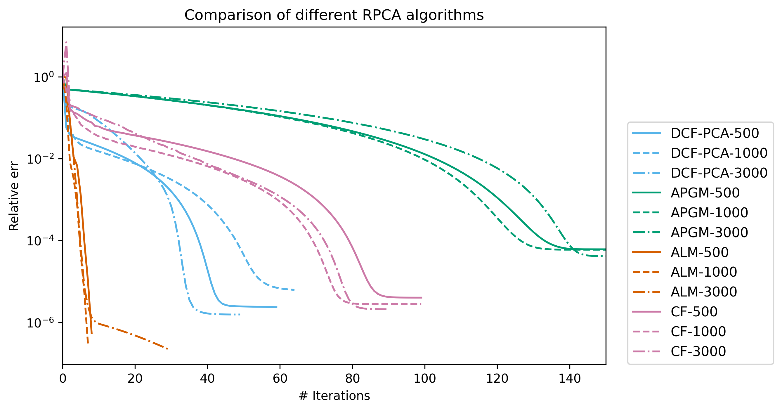
Figure 1: Comparison on the convergence of different algorithms for the synthetic RPCA problems of different scales ($m=n=500,1000,3000$).

We also test the performance of DCF-PCA on matrices with different levels of sparsity and low rank. In Figure 2 we report the relative error of the recovered matrices for different problem configurations, including $s\in[0.05,0.3]$ and $r\in[0.05n,0.2n]$. We run DCF-PCA with less than 50 iterations with $K=2$ and initial learning rate $\eta_{0}=0.05$. A distinctive limit occurs at $r\approx 0.15n$ and $s\approx 0.2$. Any target matrix with larger ground truth rank $r$ and larger sparsity $s$ than the limit cannot be recovered correctly.

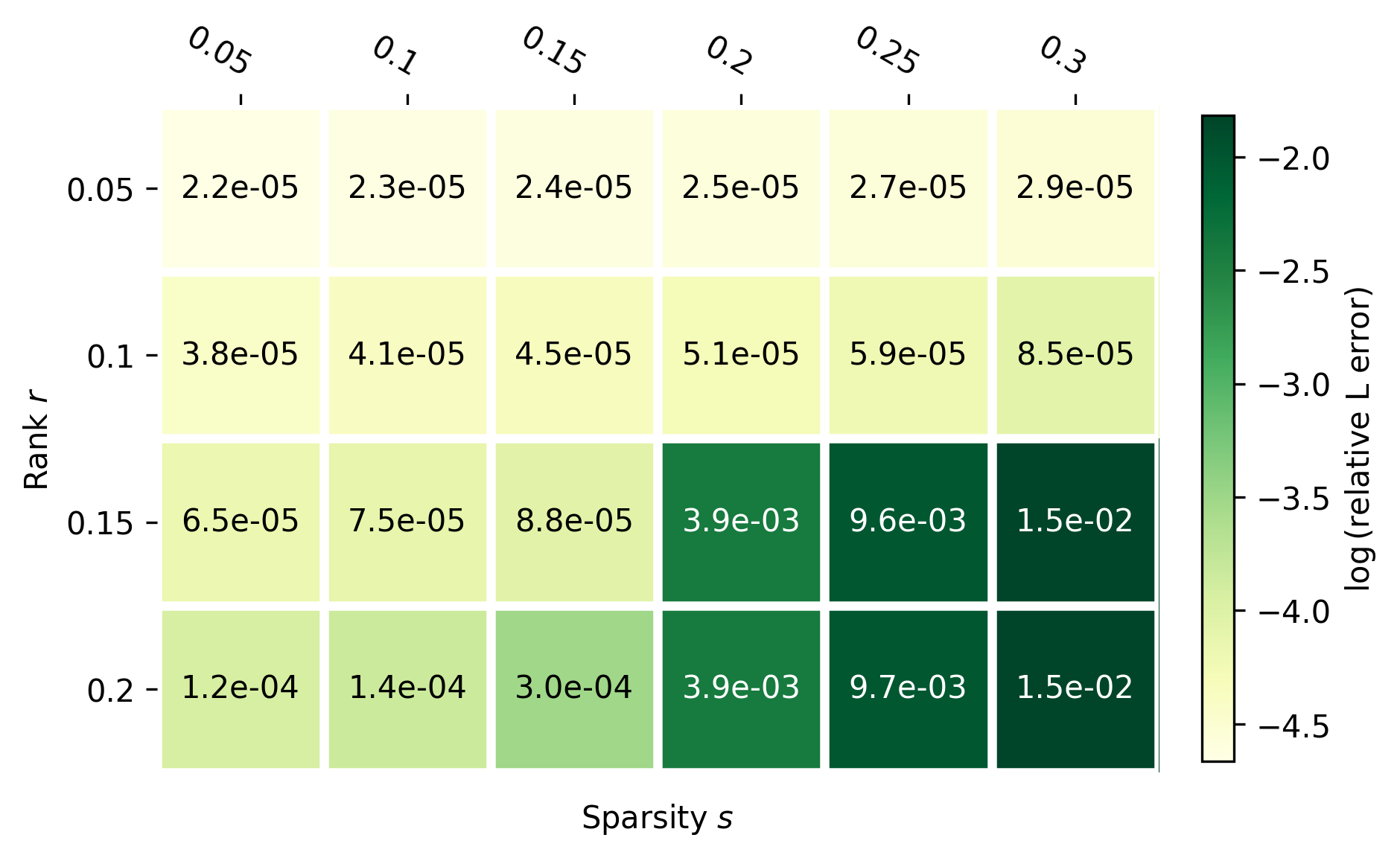
Figure 2: Relative error of the recovered matrices under different sparsity and low-rank levels (m=n=500).

Upper-bound rank recovery

Here we present the evaluation results for DCF-PCA without anticipating the exact rank of $L$, but only with an upper bound $r\leq p$ on the rank. Figure 3 compares the singular values of the recovered matrix $L^{(T)}$ with the original low-rank matrix $L_{0}$, when $M=N=200$, $r=0.05n,s=0.05$ and $p=0.1n$. It shows that the recovered matrix with $p=2r$ successfully approximate the ground truth matrix of rank $r$, as $\sigma_{r+1}(L^{(T)})/\sigma_{r}(L^{(T)})$ is small. Quantitatively, we report the relative singular value error: $\frac{\max|\sigma_{i}(L^{(T)})-\sigma_{i}(L_{0})|}{\sigma_{r}(L_{0})}$ in Table 1 for various problem scales.

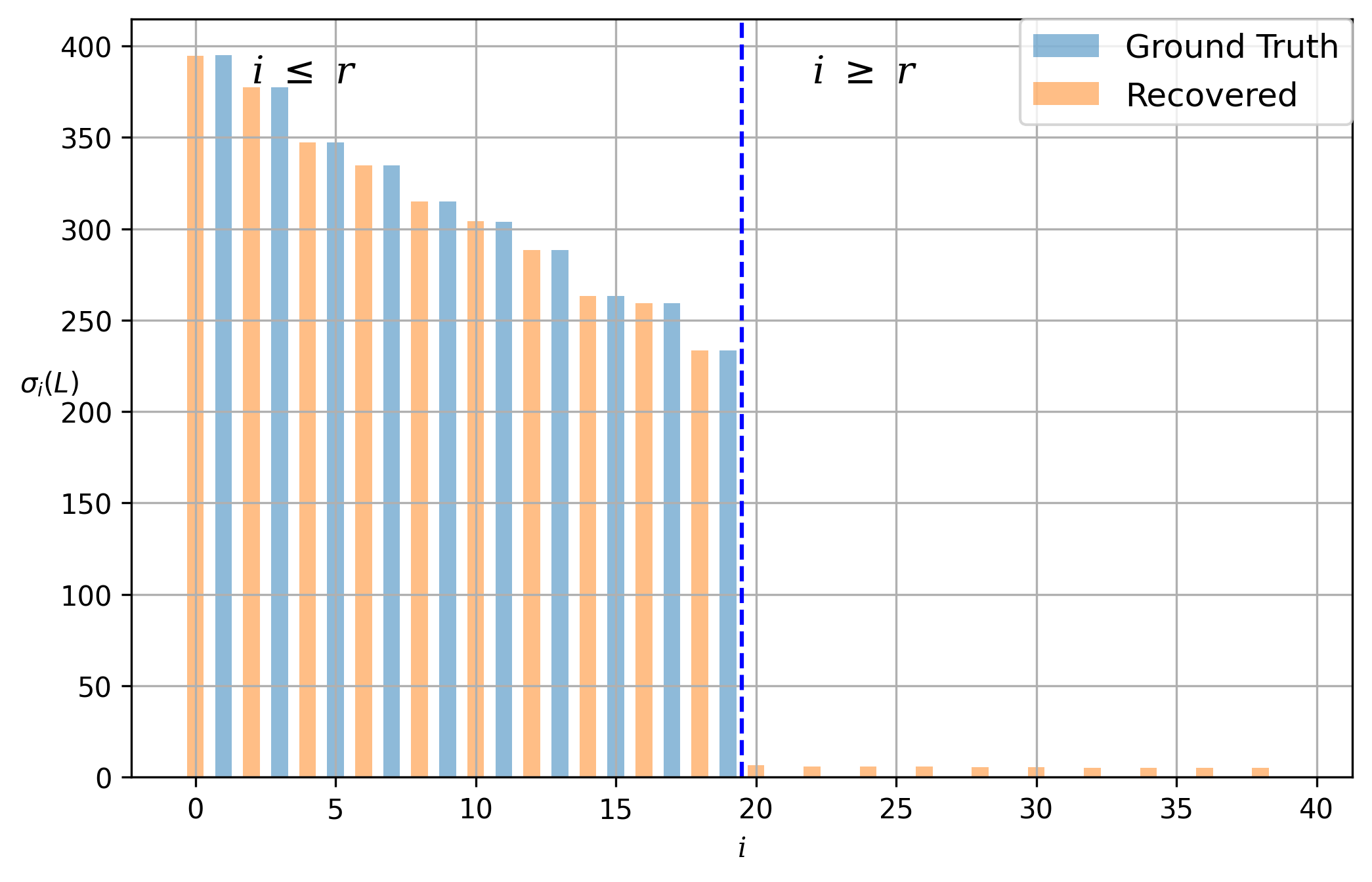
Figure 3: Comparison of the singular values between the recovered matrix and the ground truth matrix.

Table 1: Relative singular value errors of DCF-PCA for different problem scales.

n	r	p	$\frac{\max|\sigma_{i}(L^{(T)})-\sigma_{i}(L_{0})|}{\sigma_{r}(L_{0})}$
200	10	20	0.0286
500	25	50	0.0326
1000	50	100	0.0398
5000	250	500	0.1127

4.3 Ablation Studies

Number of local iterations

We study the influence of different $K$ values in DCF-PCA to the convergence rate. As $K$ denotes the number of local iterations per communication round, it reflects the level of asynchronization among remote clients. When $K=1$, the DCF-PCA algorithm is fully synchronized and $U$ descends exactly along the gradient of the global objective.

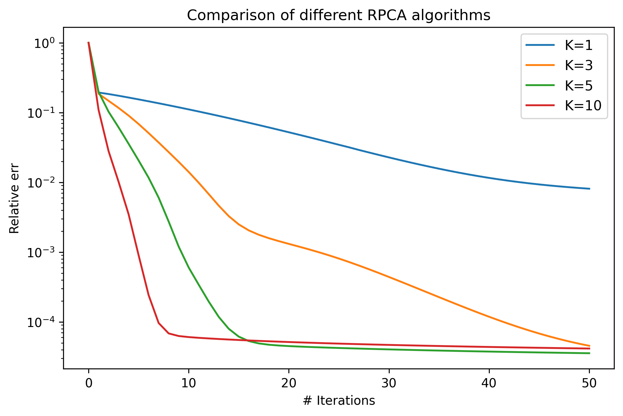
Figure 4: Comparison on different numbers of local iterations $K$. It only takes 8 iterations for DCF-PCA with $K=10$ to converge; while $K=1$ converges much slower.

Figure 4 shows the convergence of DCF-PCA with the same learning rate $\eta=0.01$ and the number of clients $E=10$, but with different values of $K$. Our algorithm converges remarkably faster as $K$ increases, but also suffers from a slightly larger error floor at the same time.

5 Conclusions

In this work we formalize the problem of distributed robust principal analysis and present a distributed consensus-factorization algorithm (DCF-PCA) that can run distributedly in remote devices. Our algorithm does not require sharing the target matrices among remote clients and only consumes limited communication. The nice properties of DCF-PCA help preserving private data of clients and speeding up the computation of large-scale RPCA problems. DCF-PCA is particularly effective for scenarios when $n$ represents the total number of items in a large distributed dataset while $m$ represents the data dimension or the extracted features dimension in deep learning applications, since $n\gg m$ is usually observed in these cases. We show the convergence of our algorithm both theoretically and numerically. DCF-PCA is also shown not sensitive to the choices of the number of local iterations $K$ and predefined rank upper bound $p$.

Appendix A Omitted Preliminaries

A.1 Additional Lemmas

Danskin’s Theorem

Here we recall a finer version of the Danskin’s Theorem as stated in [11].

Lemma 5 (Theorem 4.1 [11]).

Let $f:\mathbb{R}^{a}\times\mathbb{R}^{b}\to\mathbb{R}$. Suppose $f(x,\cdot)$ is differentiable and that $f(x,u),\nabla_{u}f(x,u)$ are continuous. Let $\Phi\subseteq\mathbb{R}^{a}$ be a compact subset. Then $g(u)=\min_{x\in\Phi}f(x,u)$ is directionally differentiable. Moreover, when $f(\cdot,u)$ has a unique minimizer $x^{*}$ over $\Phi$,

$$\nabla_{u}g(u)=\nabla_{u}f(x,u).$$ (31)

A.2 Huber Loss

The huber loss $H_{\lambda}(\cdot)$ is defined as

$$H_{\lambda}(x)=\begin{cases}-\lambda x-\frac{\lambda^{2}}{2},\quad\text{if}\ x<-\lambda.\\ \frac{x^{2}}{2},\quad\text{if}\ -\lambda\leq x\leq\lambda\\ \lambda x-\frac{\lambda^{2}}{2},\quad\text{if}\ x>\lambda.\end{cases}$$ (32)

One can quickly check that $H_{\lambda}(x)$ is convex and differentiable. Furthermore, if $X\in\mathbb{R}^{m\times n}$ is a matrix, we define $H_{\lambda}(X)=\sum_{i=1}^{m}\sum_{j=1}^{n}H_{\lambda}(X_{ij})$.

A.3 Incoherence condition

The general problem formulation for robust PCA is ill-posed. It assumes the target matrix $M$ can be decomposed to a low-rank matrix $L$ and a sparse matrix $S$, but there might be multiple possible solutions to it. Moreover, when $L$ is also sparse or $S$ has low rank, the recovery process is meaningless. [7] presents the incoherence conditions for RPCA problems that guarantees $L$ to be dense enough and $S$ to have larger enough rank, so that the recovery by optimizing convex relaxed objective Equation 2 is exact. The incoherence condition is stated as

$$\max_{i}\|U^{T}e_{i}\|^{2}\leq\frac{\delta r}{m},\max_{i}\|V^{T}e_{i}\|^{2}\leq\frac{\delta r}{n}$$ (33)

$$\|UV^{T}\|_{\infty}\leq\sqrt{\frac{\delta r}{mn}}.$$ (34)

where $L=U\Sigma V^{T}$ is the singular value decomposition of $L$. Later, it is shown that under this assumption, Equation 3 also recovers $L$ with high probability.

Appendix B Proofs

B.1 Deferred Proofs of Lemmas

Lemma 1.

Proof.

Note that the Huber loss function $H_{\lambda}(\cdot)$ is differentiable, so

$$\nabla_{V_{i}}h(V_{i})=\rho V_{i}+H_{\lambda}^{\prime}(M_{i}-UV_{i}^{T})^{T}U.$$ (35)

For any $V_{1},V_{2}\in\mathbb{R}^{n_{i}\times r}$, we have

$$\|\nabla h(V_{1})-\nabla h(V_{2})\|_{F} =\|\rho(V_{1}-V_{2})+U\left(H_{\lambda}^{\prime}(M_{i}-UV_{1}^{T})-H_{\lambda}^{\prime}(M_{i}-UV_{2}^{\prime})\right)\|_{F}$$ (36)

$$\leq\rho\|V_{1}-V_{2}\|_{F}+\|U\|_{F}\|H_{\lambda}^{\prime}(M_{i}-UV_{1}^{T})-H_{\lambda}^{\prime}(M_{i}-UV_{2}^{T})\|_{F}$$ (37)

$$\leq\rho\|V_{1}-V_{2}\|_{F}+\|U\|_{F}\|UV_{1}^{T}-UV_{2}^{T}\|_{F}$$ (38)

$$\leq(\rho+C_{U}^{2})\|V_{1}-V_{2}\|_{F}.$$ (39)

so $h(\cdot)$ is $(\rho+C_{U}^{2})$-smooth. On the other hand, $f(V_{i},S_{i})=\frac{1}{2}\|UV_{i}^{T}+S_{i}-M_{i}\|_{F}^{2}+\lambda\|S_{i}\|_{1}$ is convex, so

$$h(V_{i})=\frac{\rho}{2}\|V_{i}\|_{F}^{2}+\min_{S_{i}}f(V_{i},S_{i})$$ (40)

is $\rho$-strongly convex. ∎

Lemma 2.

Proof.

Recall that the local objective function is defined as

$$\mathcal{L}_{i}(U,V_{i},S_{i})=\frac{1}{2}\|UV_{i}^{T}+S_{i}-M_{i}\|^{2}_{F}+\frac{\rho}{2}(\frac{n_{i}}{n}\|U\|_{F}^{2}+\|V_{i}\|_{F}^{2})+\lambda\|S_{i}\|_{1}.$$

It is clear that $\mathcal{L}(\cdot,V_{i},S_{i})$ is differentiable. Moreover, both $\mathcal{L}$ and $\nabla_{U}L(U,V_{i},S_{i})=\frac{\rho n_{i}}{n}U+(UV_{i}^{T}+S_{i}-M)V_{i}$ are continuous. We also know that for any fixed $U$, $\arg\min_{V_{i},S_{i}}\mathcal{L}(U,V_{i},S_{i})$ is unique, since $h(V_{i})$ is $\rho$-strongly convex. Therefore, according to Lemma 5, $g_{i}(U)=\nabla_{U}\nabla_{U}\mathcal{L}(U,V_{i},S_{i})$.

∎

Lemma 3.

Proof.

Let $V_{i}^{*},S_{i}^{*}=\arg\min_{V_{i},S_{i}}\mathcal{L}(U,V_{i},S_{i})$

$$\nabla_{U}g_{i}(U) =\nabla_{U}\min_{V_{i},S_{i}}\mathcal{L}(U,V_{i},S_{i})$$ (41)

$$=\nabla_{U}\mathcal{L}(U,V_{i}^{*},S_{i}^{*})$$ (42)

Note that $\mathcal{L}(U,V,S)$ is strongly convex in terms of $V$ and $S$, we have

$$\mathcal{L}_{i}(U,V_{i}^{\prime},S_{i}^{\prime})-\mathcal{L}_{i}(U,V_{i},S_{i})\geq\frac{\rho}{2}\|V^{\prime}-V\|_{F}^{2}+\frac{1}{2}\|S^{\prime}-S\|_{F}^{2}.$$ (43)

Similarly,

$$\mathcal{L}_{i}(U^{\prime},V_{i},S_{i})-\mathcal{L}_{i}(U^{\prime},V_{i}^{\prime},S_{i}^{\prime})\geq\frac{\rho}{2}\|V^{\prime}-V\|_{F}^{2}+\frac{1}{2}\|S^{\prime}-S\|_{F}^{2}.$$ (44)

On the other hand,

$$f(V_{i},S_{i})=\mathcal{L}(U^{\prime},V_{i},S_{i})-\mathcal{L}(U,V_{i},S_{i})$$ (45)

is Lipschitz in terms of $V_{i}$ and $S_{i}$. This is because

$$\|\frac{\partial f}{\partial V_{i}}\|_{F}=\|V_{i}({U^{\prime}}^{T}U^{\prime}-U^{T}U)\|_{F}\leq C_{V}\|{U^{\prime}}^{T}U^{\prime}-U^{T}U\|_{F}\leq 2C_{V}C_{U}\|U^{\prime}-U\|_{F}$$ (46)

$$\|\frac{\partial f}{\partial S_{i}}\|_{F}=\|(U^{\prime}-U)V_{i}\|_{F}\leq C_{V}\|U^{\prime}-U\|_{F}.$$ (47)

Therefore,

$$f(V_{i}^{\prime},S_{i}^{\prime})-f(V_{i},S_{i})\leq 2C_{V}C_{U}(\|V_{i}^{\prime}-V_{i}\|_{F}+\|S_{i}^{\prime}-S_{i}\|_{F}).$$ (48)

and

$$f(V_{i}^{\prime},S_{i}^{\prime})-f(V_{i},S_{i})\geq\frac{\rho}{2}(\|V^{\prime}-V\|_{F}^{2}+\|S^{\prime}-S\|_{F}^{2}).$$ (49)

Combine these two inequalities, we have

$$\|V_{i}^{\prime}-V_{i}\|_{F}+\|S_{i}^{\prime}-S_{i}\|_{F}\leq\frac{4C_{V}C_{U}}{\rho}\|U^{\prime}-U\|_{F}.$$ (50)

Now

$$\|\nabla g_{i}(U^{\prime})-\nabla g_{i}(U)\|_{F} \leq\|U_{i}^{\prime}-U\|_{F}\|{V_{i}^{\prime}}^{T}V_{i}^{\prime}+\frac{n_{i}}{n}I\|_{F}+\|S^{\prime}V_{i}^{\prime}-SV_{i}\|_{F}$$

$$\hskip 70.0001pt+\|M_{i}(V_{i}^{\prime}-V_{i})\|_{F}+\|U\|_{F}\|{V_{i}^{\prime}}^{T}V_{i}^{\prime}-V_{i}^{T}V_{i}\|_{F}$$ (51)

$$\leq\|U^{\prime}-U\|_{F}\left(\frac{rn_{i}}{n}+C_{V}^{2}+4\frac{(C_{S}+C_{V}+\|M_{i}\|_{F})C_{V}C_{U}}{\rho}+\frac{8C_{V}^{2}C_{U}}{\rho}\right)$$ (52)

$$\leq\|U^{\prime}-U\|_{F}\left(r+C_{V}^{2}+\frac{4C_{S}+12C_{V}+4C_{M}}{\rho}C_{V}C_{U}\right)$$ (53)

∎

Lemma 4.

Proof.

The gradient of the local objective $g_{i}(U)$ is

$$\nabla_{U}g_{i}(U) =\nabla_{U}\mathcal{L}(U,V_{i}^{*},S_{i}^{*})$$ (54)

$$=(U{V_{i}^{*}}^{T}+S_{i}^{*}-M_{i})V_{i}^{*}+\frac{n_{i}}{n}U.$$ (55)

Recall that

$$(U^{T}U+\rho I){V_{i}^{*}}^{T}=U^{T}(M_{i}-S_{i}^{*})$$ (56)

$$S_{i}^{*}=\mathrm{sign}(M_{i}-U{V_{i}^{*}}^{T})\cdot\max(|M_{i}-U{V_{i}^{*}}^{T}|-\lambda,0)$$ (57)

Let $\Lambda=M_{i}-U{V_{i}^{*}}^{T}-S_{i}^{*}$, so $\|\Lambda\|_{\infty}\leq\lambda$. Then Equation 56 can be rewritten as

$$\rho V_{i}^{*}=\Lambda^{T}U$$ (58)

Bringing this back to Equation 55 yields

$$\nabla_{U}g_{i}(U)=-\Lambda V_{i}^{*}+\frac{n_{i}}{n}U=(\frac{n_{i}}{n}I_{m}-\Lambda\Lambda^{T})U$$ (59)

Since $\|\Lambda\Lambda^{T}\|_{F}^{2}\leq m^{2}n\lambda^{2}$,

$$\|\nabla_{U}g_{i}(U)\|_{F}\leq\sqrt{(\frac{n_{i}^{2}}{n^{2}}m\rho^{2}+m^{2}n_{i}\lambda^{2})}\|U\|_{F}\leq C_{U}\sqrt{\frac{n_{i}^{2}m\rho^{2}}{n^{2}}+m^{2}n_{i}\lambda^{2}}.$$ (60)

∎

B.2 Proof for Theorem 1

Proof.

We first recall a theorem proved in [8]:

Lemma 6 (Yu et al. [8] Theorem 1).

Suppose each local objective function is $L$-smooth and has bounded gradient norm $\|\nabla f_{i}(w)\|_{2}\leq G$. If each local agent runs local SGD and synchronizes their model weights every $K$ iterations, the FedAvg algorithm converges with

$$\frac{1}{T}\sum_{i=1}^{T}\mathbb{E}[\|\nabla f(w^{(t)})\|^{2}]\leq\frac{2}{\eta T}(f(w^{(0)}-f^{*}))+4\eta^{2}K^{2}G^{2}L^{2}+\frac{L}{N}\eta\sigma.$$ (61)

where the learning rate $\eta\leq\frac{1}{L}$ and $\sigma$ is the variance of each SGD update.

Notice that our DCF-PCA algorithm has no variance in each local update. We combine Lemmas 3, 4 and 6 by $G\leq C_{U}\sqrt{m\rho^{2}+m^{2}n\lambda^{2}}$ and derive the result of Theorem 1.

∎

References

- [1] Jiashi Feng, Huan Xu, and Shuicheng Yan. Online robust pca via stochastic optimization. In NIPS, 2013.
- [2] Benjamin Recht, Maryam Fazel, and Pablo A. Parrilo. Guaranteed minimum-rank solutions of linear matrix equations via nuclear norm minimization. SIAM Review, 52(3):471–501, jan 2010.
- [3] Brendan McMahan, Eider Moore, Daniel Ramage, Seth Hampson, and Blaise Aguera y Arcas. Communication-Efficient Learning of Deep Networks from Decentralized Data. In Aarti Singh and Jerry Zhu, editors, Proceedings of the 20th International Conference on Artificial Intelligence and Statistics, volume 54 of Proceedings of Machine Learning Research, pages 1273–1282. PMLR, 20–22 Apr 2017.
- [4] Xiang Li, Kaixuan Huang, Wenhao Yang, Shusen Wang, and Zhihua Zhang. On the convergence of fedavg on non-iid data. In International Conference on Learning Representations, 2020.
- [5] Farzin Haddadpour and Mehrdad Mahdavi. On the convergence of local descent methods in federated learning. CoRR, abs/1910.14425, 2019.
- [6] Ningyu Sha, Lei Shi, and Ming Yan. Fast algorithms for robust principal component analysis with an upper bound on the rank. Inverse Problems and Imaging, 15(1):109–128, 2021.
- [7] Emmanuel J. Candès, Xiaodong Li, Yi Ma, and John Wright. Robust principal component analysis? J. ACM, 58(3), jun 2011.
- [8] Hao Yu, Sen Yang, and Shenghuo Zhu. Parallel restarted sgd with faster convergence and less communication: Demystifying why model averaging works for deep learning. In AAAI, 2019.
- [9] Zhouchen Lin, Arvind Ganesh, John Wright, Leqin Wu, Minming Chen, and Yi Ma. Fast convex optimization algorithms for exact recovery of a corrupted low-rank matrix. 2009.
- [10] Donald Goldfarb, Shiqian Ma, and Katya Scheinberg. Fast alternating linearization methods for minimizing the sum of two convex functions. Mathematical Programming, 141:349–382, 2013.
- [11] J. Frédéric Bonnans and Alexander Shapiro. Optimization problems with perturbations: A guided tour. SIAM Review, 40(2):228–264, 1998.