Training Robust Spiking Neural Networks on Neuromorphic Data with Spatiotemporal Fragments

Abstract

Neuromorphic vision sensors (event cameras) are inherently suitable for spiking neural networks (SNNs) and provide novel neuromorphic vision data for this biomimetic model. Due to the spatiotemporal characteristics, novel data augmentations are required to process the unconventional visual signals of these cameras. In this paper, we propose a novel Event SpatioTemporal Fragments (ESTF) augmentation method. It preserves the continuity of neuromorphic data by drifting or inverting fragments of the spatiotemporal event stream to simulate the disturbance of brightness variations, leading to more robust spiking neural networks. Extensive experiments are performed on prevailing neuromorphic datasets. It turns out that ESTF provides substantial improvements over pure geometric transformations and outperforms other event data augmentation methods. It is worth noting that the SNNs with ESTF achieve the state-of-the-art accuracy of 83.9% on the CIFAR10-DVS dataset.

Index Terms—  Spiking Neural Networks, Event Spatiotemporal Fragment Augmentation, Neuromorphic Data

1 Introduction

Event cameras [1, 2] are bio-inspired vision sensors that operate in a completely different way from traditional cameras [3, 4]. Instead of capturing images at a fixed rate, the cameras asynchronously measure per-pixel brightness changes and output a stream of events that encode the time, location, and sign of the brightness changes. Since both events and spikes are modeled from neural signals, event cameras are inherently suitable for spiking neural networks (SNNs), which are considered promising models for artificial intelligence (AI) and theoretical neuroscience [5].

Due to the event characteristics, brightness variances tend to disrupt the spatiotemporal positions of the events, posing a great challenge to the robustness of SNNs. However, traditional data augmentations are fundamentally designed for RGB data and lack exploration of neuromorphic events, such as mixup [6] and random erase [7]. Therefore, novel data augmentations are required to process the unconventional visual signals of these cameras.

In this paper, we propose a novel Event SpatioTemporal Fragments (ESTF) augmentation method to model the effects of brightness variances on neuromorphic data. ESTF can be simply summarized into two components, inverting event fragments in the spatiotemporal and polarity domains, and drift events in the spatiotemporal domain. ESTF preserves the original spatiotemporal structure through transformed fragments and increases the diversity of neuromorphic data. Extensive experiments are conducted on prevailing neuromorphic datasets. It turns out that ESTF improves the robustness of SNNs by simulating the effect of brightness variances on neuromorphic data. Furthermore, we analyze the insightful superiority of ESTF compared with other event data augmentation methods. It is worth noting that ESTF is super effective on both SNNs and convolutional neural networks (CNNs). For example, the SNNs with ESTF yield a substantial improvement over previous state-of-the-art results and achieve an accuracy of 83.9% on the CIFAR10-DVS dataset, which illustrates the importance of event spatiotemporal fragment augmentation.

In addition, while this work is related to EventDrop [8] and NDA [9], there are some distinct differences. For example, NDA is a purely global geometric transformation, while ESTF transforms partial event stream in the spatiotemporal or polarity domain. EventDrop introduces noise by dropping events, resulting in poor sample continuity. However, ESTF also considers the brightness variances in neuromorphic data and preserves the original spatiotemporal structure of events.

2 Method

2.1 Event Generation Model

The event generation model [3, 4] is abstracted from dynamic vision sensors [2]. Each pixel of the event camera responds to changes in its logarithmic photocurrent $L=\log(I)$. Specifically, in a noise-free scenario, an event $e_{k}=(x_{k},y_{k},t_{k},p_{k})$ is triggered at pixel $X_{k}=(y_{k},x_{k})$ and at time $t_{k}$ as soon as the brightness variation $|\Delta L|$ reaches a temporal contrast threshold $C$ since the last event at the pixel. The event generation model can be expressed by the following formula:

$$\Delta L(X_{k},t_{k})=L(X_{k},t_{k})-L(X_{k},t_{k}-\Delta t_{k})=p_{k}C$$ (1)

where $C>0$, $\Delta t_{k}$ is the time elapsed since the last event at the same pixel, and the polarity $p_{k}\in\{+1,-1\}$ is the sign of the brightness change. During a period, the event camera triggers event stream $\mathcal{E}$:

$$\mathcal{E}=\left\{e_{k}\right\}_{k=1}^{N}=\left\{\left(X_{k},t_{k},p_{k}\right)\right\}_{k=1}^{N}$$ (2)

where $N$ represents the number of events in the set $\mathcal{E}$.

Further, inspired by previous work [3], an event field is used to represent the discrete $\mathcal{E}$ by replacing each event of the spatiotemporal stream with a Dirac spike, resulting in a continuous representation of events. For convenience, we define the complete set of transformation domains as $D=\{X,p,t\}$, and map the polarity $p$ from $\{-1,+1\}$ to $\{0,1\}$. The continuous event filed $S$ can be expressed as the following formula:

$$S^{\mathcal{E}}(X,p,t) =\sum_{e_{k}\in\mathcal{E}}\delta(X-X_{k})\delta(t-t_{k})\delta(p-p_{k})$$ (3)

$$=\sum_{e_{k}\in\mathcal{E}}\prod_{i\in D}\delta\left(i-i_{k}\right)$$

The event generation model is shown in Fig. 1(a), an event is generated each time the brightness variances reach the threshold, and then $|\Delta L|$ is cleared. Note that due to the single-ended inverting amplifier in the sensor differential circuit, the threshold for brightness changes in the circuit is one sign different from the threshold in the conceptual model. In addition, the short segment following the firing event represents the corresponding refractory period in biological neurons.

2.2 Motivation

This work stems from three observations. First, the mammalian brain can make correct judgments based on fragments of time and space, while SNNs are less robust. In addition, it can be known from the event generation model that events asynchronously record brightness variances in microseconds. Thus, even slight brightness variances can disrupt the time or polarity of events, leading to cascading changes in subsequent events. As shown in Figures 1(b),  1(c), and  1(d), microsecond-level fluctuations in brightness can disrupt the spatiotemporal position and even the polarity of event fragments. Furthermore, sensor noise not only discards events [8], but may also disrupt the spatiotemporal location of event fragments. For example, jitter in the step response may introduce sensor delays [2], resulting in delayed brightness variances. The relative mismatch between the reset level of the differential circuit and the comparator threshold may lead to a mismatch in the dynamic threshold $C$ [2], causing the effect shown in Fig. 1(d). These observations inspire us to improve the robustness of SNNs by artificially generating event spatiotemporal fragments.

(a) Event generation model.

(b) Opposite light-dark processes.

(c) Inverted brightness variations.

(d) Delayed brightness variations.

Fig. 1: The relationship between logarithmic intensity and events generation for each pixel. (a) is the initial brightness and (b)(c)(d) is the changed brightness.

2.3 Event SpatioTemporal Fragment Augmentation

To obtain the transformed event spatiotemporal fragments, the ESTF method is divided into two parts, inverting event fragments in spatiotemporal or polarity domains (ISTP), and drifting event fragments in spatiotemporal domain (DST).

ISTP refers to inverting certain event fragments $\mathcal{E}_{c}$ on spatiotemporal or polarity domains $d$. The transformed event field $S_{ISTP}$ can be formulated as:

$$S^{\mathcal{E}_{c}}_{ISTP}(X,p,t) =\sum_{e_{k}\in\mathcal{E}_{c}}(\delta\left(d+d_{k}-R_{d}\right)\prod_{i\in D\{d\}}\delta\left(i-i_{k}\right))$$ (4)

where $d\in D$, $R_{d}$ represents the resolution of the domain $d$. Event fragments are inverted from $d_{k}$ to their symmetrical positions $R_{d}-d_{k}$ in the event stream. When $d$ is the time domain $t$, $R_{d}$ represents the largest timestamp, when $d$ is the polarity $p$, $R_{d}$ represents 1, and when $d$ is the space coordinate $X$, $R_{d}$ represents the image resolution. $D\{d\}$ is the complement of $d$ with respect to $D$.

Table 1: Performance of ESTF method and the SOTAs on CIFAR10-DVS, N-Caltech101 and N-CARS datasets.

Network	Method	Reference	Model	CIFAR10-DVS	N-Caltech101	N-CARS
CNNs-based	RG-CNNs [10]	TIP 2020	Graph-CNN	54.00	61.70	91.40
	SlideGCN [11]	ICCV 2021	Graph-CNN	68.00	76.10	93.10
	EventDrop [8]	IJCAI 2021	Mobilenet-V2	-	87.14	94.55
	ECSNet [12]	T-CSVT 2022	LEE$\rightarrow$MA	72.70	69.30	94.60
	EV-VGCNN [13]	CVPR 2022	EV-VGCNN	67.00	74.80	95.30
	NDA [9]	ECCV 2022	Resnet-34	-	81.20	95.50
	Ours(w/o. ESTF)	-	Resnet-34	77.15	90.86	93.80
	Ours(w/. ESTF)	-	Resnet-34	83.12+5.97	93.15+2.29	96.00+2.20
SNNs-based	HATS[14]	CVPR 2018	HATS-SVM	52.40	64.20	81.0
	Dart[15]	TPAMI 2020	SPM-SVM	65.80	66.80	-
	STBP [16]	AAAI 2021	Resnet-19	67.80	-	-
	Dspike [17]	NeurIPS 2021	ResNet-18	75.40	-	-
	AutoSNN [18]	ICML 2022	-	72.50	-	-
	RecDis [19]	CVPR 2022	Resnet-19	72.42	-	-
	DSR [20]	CVPR 2022	VGG-11	77.27	-	-
	NDA [9]	ECCV 2022	VGG-11	81.70	78.20	90.1
	Ours(w/o. ESTF)	-	VGG-9	67.70	67.32	91.65
	Ours(w/. ESTF)	-	VGG-9	83.90+16.20	80.07+12.75	95.64+3.99

DST drifts events $\mathcal{E}_{c}$ a certain distance on spatiotemporal domain, which can be represented as a convolution kernel $k_{DST}$:

$$k_{DST}(X,p,t)=\delta\left(d-r_{d}\right)\prod_{i\in D\{d\}}\delta\left(i\right)$$ (5)

where $d\in\{X,t\}$, $r_{d}$ represents the moving distance in the domain $d$. The transformed event field $S_{DST}$ can be obtained by convolving $k_{DST}$ with the event field $S$:

$$S^{\mathcal{E}_{c}}_{DST}(X,p,t) =\left(k_{DST}*S\right)(X,p,t)$$ (6)

$$=\sum_{e_{k}\in\mathcal{E}_{c}}k_{DST}(X-X_{k},p-p_{k},t-t_{k})$$

$$=\sum_{e_{k}\in\mathcal{E}_{c}}(\delta\left(d-d_{k}-r_{d}\right)\prod_{i\in D\{d\}}\delta\left(i-i_{k}\right))$$

where $d\in\{X,t\}$ and $\mathcal{E}_{c}$ represents events to be drifted. DST drifts fragments $\mathcal{E}_{c}$ a distance $r$ in the domain $d$, and the part beyond borders will be discarded. It is worth noting that drifted samples of different scales are generated by different distances $r$, which obey a uniform distribution specified by a hyperparameter. In addition, the event field $S_{ESTF}$ that applies both ISTP and DST can be obtained by convolving $k_{DST}$ and $S_{ISTP}$:

$$S^{\mathcal{E}_{c}}_{ESTF}(X,p,t)=\left(k_{DST}*S^{\mathcal{E}_{c}}_{ISTP}\right)(X,p,t)$$ (7)

The pseudocode of ESTF is given by Algorithm 1.

Algorithm 1 ESTF Procedure

Input: Original events $S=\left\{e_{i}\right\}_{i=1}^{N}$
Parameter: Fragments ratio $c_{istp}$ and $c_{dst}$; Domain: $d_{istp}$ and $d_{dst}$; Drift ratio: $r$; Resolution: $R_{d}$.
Output: Transformed event fragments $\mathcal{S}_{ESTF}$

1:  $begin\leftarrow Rand(0,1-c_{istp})$

2:  $\mathcal{E}_{i}\leftarrow\{e_{i}\}_{i\in[N*begin,N*(begin+c)]}$

3:  $S_{ISTP}=Eq4(\mathcal{E}_{i},d_{istp},R_{d})+\mathcal{E}\{\mathcal{E}_{i}\}$

4:  $begin\leftarrow Rand(0,1-c_{dst})$

5:  $\hat{r}\leftarrow Randint[-r*R_{d},r*R_{d}]$ 

6:  $\mathcal{E}_{d}\leftarrow\{e_{i}\}_{i\in[N*begin,N*(begin+c)]}$

7:  $S_{ESTF}=Eq7(S^{\mathcal{E}_{d}}_{ISTP},d_{dst},\hat{r})+\mathcal{E}\{\mathcal{E}_{d}\}$

8:  return $S_{ESTF}$

3 Experiments

3.1 Implementation

Extensive experiments are performed to demonstrate the superiority of our ESTF method on the prevailing neuromorphic datasets, including CIFAR10-DVS [21], N-Caltech101 [22], N-CARS [14] datasets. For the convenience of comparison, the model with the same parameters without ESTF is used as the baseline. STBP [16] method is used to train SNNs, and other parameters mainly refer to NDA [9]. For example, the initial learning rate is $1e-3$, the neuron threshold and leakage coefficient are 1 and 0.5, respectively. Furthermore, we also evaluate the performance of ESTF on CNNs, a popular network for processing neuromorphic data. The EST [3] representation method is used to convert neuromorphic data into a form compatible with CNNs. Adam optimizer is used with an initial learning rate of $1e-4$.

3.2 Compared with SOTAs

ESTF outperforms previous SOTAs on three prevailing and challenging neuromorphic datasets. As shown in Tab. 1, ESTF achieves substantial improvements on SNNs through spatiotemporal fragments. In particular, ESTF achieves a 16.2% improvement on the CIFAR10-DVS dataset, reaching a state-of-the-art accuracy of 83.9%. In addition, ESTF also has significant improvements over CNNs. Since ESTF is orthogonal to most training algorithms, it can provide a better baseline and improve the performance of existing models.

Table 2: Performance of ESTF compared with other event data augmentations on the N-Caltech101 dataset.

Methods	Accuracy(%)
	VGG-9	VGG-19	Resnet-34
	(SNNs)	(ANNs)	(ANNs)
Baseline	67.32	87.30	90.86
EventDrop	68.69	88.31	92.06
NDA∗	77.44	88.84	92.42
ESTF	80.07+12.75	91.29+3.99	93.15+2.29

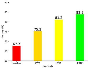
(a) ISTP and DST.

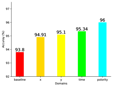
(b) Different domains.

Fig. 2: Ablation studies on ESTF.

3.3 Compared with Event Data Augmentations

As shown in Tab. 2, ESTF is compared with other reproduced event data augmentations at the same baseline. EventDrop [8] is similar to Cutout on event data and achieves remarkable success on CNNs. NDA^∗ represents applying the two naive geometric transformations flipping and translation on event data. It turns out that ESTF outperforms EventDrop and NDA^∗ in multiple networks, covering both SNNs and ANNs. It is worth noting that the performance of EventDrop in SNNs may lag far behind ESTF because deletion destroys the continuity of neuromorphic data and may cause the “dead neuron” problem. In addition, ESTF is more stable and more effective than geometric transformations. It illustrates the superiority of spatiotemporal fragment augmentation.

3.4 Ablation Studies on ESTF

Performance of ISTP and DST. As shown in Fig. 2(a), the performance of ISTP and DST are evaluated on the DVS-CIFAR10 dataset. It turns out that both ISTP and DST have significant improvements. Notably, the improvement of DST is more pronounced since drifting events are more common than inverting events.

Performance of Different Domains. As shown in Fig. 2(b), the performance of ESTF in different domains is evaluated on the N-CARS dataset. It turns out that ESTF is effective in the time, spatial, and polarity domains. It is worth noting that the ESTF performs better in the temporal and polarity domains than in the spatial domain, which indicates that the event spatiotemporal fragments are critical to improving the robustness of the model.

3.5 Analysis of ESTF

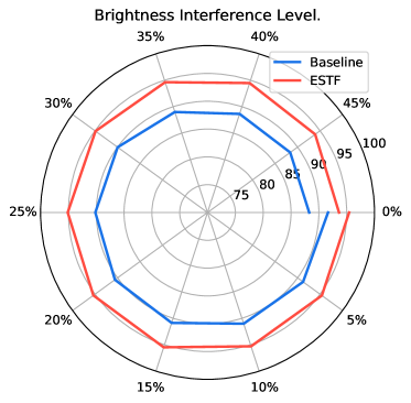
(a) Inverted brightness variations.

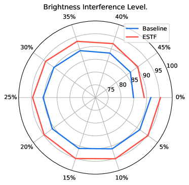
(b) Delayed brightness variations.

Fig. 3: Performance under different brightness interferences.

There are at least three insightful reasons for the superior performance of the event spatiotemporal augmentation (ESTF). Intuitively, ESTF transforms in the time, space, and polarity domains, while NDA only transforms in space. Fig 2(b) shows the performance of ESTF in different domains. It is worth noting that the effects of transformations in the time and polarity domains are significant. Considering that the performance of NDA^∗ geometric transformations is already close to SOTAs, there is still more than 2% improvement in ESTF, which is quite impressive, as shown in Tab. 2. In addition, ESTF preserves the continuity of neuromorphic data through spatiotemporal fragments, maintaining the original local features. The comparison with EventDrop in Tab. 2 illustrates the importance of continuity. Furthermore, the transformations of ISTP and DST in time and polarity domains essentially improve the robustness of SNNs to brightness variances. Note that event samples may only last 100ms (N-CARS), and slight brightness fluctuations can bring brightness variances similar to Fig. 1. As shown in Fig. 3, we further evaluate the robustness of SNNs against brightness variances. It turns out that the model with ESTF is significantly more robust under various degrees of brightness interference.

4 Conclusion

In this paper, we propose event spatiotemporal fragment augmentation. It preserves the continuity of the data, transforms events in the spatiotemporal and polarity domains, and simulates the influence of brightness variances on neuromorphic data. It makes up for the omission of spatiotemporal fragment augmentation in the past, resulting in superior improvements and SOTA performance on prevailing neuromorphic datasets.

References

- [1] Christoph Posch, Teresa Serrano-Gotarredona, Bernabé Linares-Barranco, and Tobi Delbrück, “Retinomorphic event-based vision sensors: Bioinspired cameras with spiking output,” Proc. IEEE, pp. 1470–1484, 2014.
- [2] Patrick Lichtsteiner, Christoph Posch, and Tobi Delbrück, “A 128×128 120 db 15 s latency asynchronous temporal contrast vision sensor,” IEEE J. Solid State Circuits, vol. 43, no. 2, pp. 566–576, 2008.
- [3] Daniel Gehrig, Antonio Loquercio, Konstantinos G. Derpanis, and Davide Scaramuzza, “End-to-end learning of representations for asynchronous event-based data,” in ICCV. 2019, pp. 5632–5642, IEEE.
- [4] Guillermo Gallego, Tobi Delbrück, Garrick Orchard, Chiara Bartolozzi, Brian Taba, Andrea Censi, Stefan Leutenegger, Andrew J. Davison, Jörg Conradt, Kostas Daniilidis, and Davide Scaramuzza, “Event-based vision: A survey,” TPAMI., vol. 44, no. 1, pp. 154–180, 2022.
- [5] Kaushik Roy, Akhilesh Jaiswal, and Priyadarshini Panda, “Towards spike-based machine intelligence with neuromorphic computing,” Nature, vol. 575, no. 7784, pp. 607–617, 2019.
- [6] Hongyi Zhang, Moustapha Cissé, Yann N. Dauphin, and David Lopez-Paz, “mixup: Beyond empirical risk minimization,” in ICLR. 2018, OpenReview.net.
- [7] Zhun Zhong, Liang Zheng, Guoliang Kang, Shaozi Li, and Yi Yang, “Random erasing data augmentation,” in AAAI, 2020, vol. 34, pp. 13001–13008.
- [8] Fuqiang Gu, Weicong Sng, Xuke Hu, and Fangwen Yu, “Eventdrop: Data augmentation for event-based learning,” in IJCAI. 2021, pp. 700–707, ijcai.org.
- [9] Yuhang Li, Youngeun Kim, Hyoungseob Park, Tamar Geller, and Priyadarshini Panda, “Neuromorphic data augmentation for training spiking neural networks,” arXiv preprint arXiv:2203.06145, 2022.
- [10] Yin Bi, Aaron Chadha, Alhabib Abbas, Eirina Bourtsoulatze, and Yiannis Andreopoulos, “Graph-based spatio-temporal feature learning for neuromorphic vision sensing,” IEEE Trans. Image Process., vol. 29, pp. 9084–9098, 2020.
- [11] Yijin Li, Han Zhou, Bangbang Yang, Ye Zhang, Zhaopeng Cui, Hujun Bao, and Guofeng Zhang, “Graph-based asynchronous event processing for rapid object recognition,” in International Conference on Computer Vision, ICCV. 2021, pp. 914–923, IEEE.
- [12] Zhiwen Chen, Jinjian Wu, Junhui Hou, Leida Li, Weisheng Dong, and Guangming Shi, “Ecsnet: Spatio-temporal feature learning for event camera,” IEEE Transactions on Circuits and Systems for Video Technology, pp. 1–1, 2022.
- [13] Yongjian Deng, Hao Chen, Hai Liu, and Youfu Li, “A voxel graph cnn for object classification with event cameras,” in Proceedings of the IEEE/CVF Conference on Computer Vision and Pattern Recognition, 2022, pp. 1172–1181.
- [14] Amos Sironi, Manuele Brambilla, Nicolas Bourdis, Xavier Lagorce, and Ryad Benosman, “Hats: Histograms of averaged time surfaces for robust event-based object classification,” in CVPR, June 2018.
- [15] Bharath Ramesh, Hong Yang, Garrick Orchard, and et al., “Dart: Distribution aware retinal transform for event-based cameras,” TPAMI, vol. 42, no. 11, pp. 2767–2780, 2020.
- [16] Hanle Zheng, Yujie Wu, Lei Deng, Yifan Hu, and Guoqi Li, “Going deeper with directly-trained larger spiking neural networks,” in Proceedings of the AAAI Conference on Artificial Intelligence, 2021, pp. 11062–11070.
- [17] Yuhang Li, Yufei Guo, Shanghang Zhang, Shikuang Deng, Yongqing Hai, and Shi Gu, “Differentiable spike: Rethinking gradient-descent for training spiking neural networks,” Advances in Neural Information Processing Systems, vol. 34, pp. 23426–23439, 2021.
- [18] Byunggook Na, Jisoo Mok, Seongsik Park, Dongjin Lee, Hyeokjun Choe, and Sungroh Yoon, “Autosnn: Towards energy-efficient spiking neural networks,” arXiv preprint arXiv:2201.12738, 2022.
- [19] Yufei Guo, Xinyi Tong, Yuanpei Chen, Liwen Zhang, Xiaode Liu, Zhe Ma, and Xuhui Huang, “Recdis-snn: Rectifying membrane potential distribution for directly training spiking neural networks,” in Proceedings of the IEEE/CVF Conference on Computer Vision and Pattern Recognition, 2022, pp. 326–335.
- [20] Qingyan Meng, Mingqing Xiao, Shen Yan, Yisen Wang, Zhouchen Lin, and Zhi-Quan Luo, “Training high-performance low-latency spiking neural networks by differentiation on spike representation,” in CVPR, 2022, pp. 12444–12453.
- [21] Hongmin Li, Hanchao Liu, Xiangyang Ji, and et al., “Cifar10-dvs: An event-stream dataset for object classification,” Frontiers in Neuroscience, 2017.
- [22] Garrick Orchard, Ajinkya Jayawant, Gregory Cohen, and Nitish V. Thakor, “Converting static image datasets to spiking neuromorphic datasets using saccades,” CoRR, vol. abs/1507.07629, 2015.