The discriminating power of the generalized rank invariant

Abstract

The rank invariant (RI), one of the best known invariants of persistence modules $M$ over a given poset $\mathrm{P}$, is defined as the map sending each comparable pair $p\leq q$ in $\mathrm{P}$ to the rank of the linear map $M(p\leq q)$. The recently introduced notion of generalized rank invariant (GRI) acquires more discriminating power than the RI at the expense of enlarging the domain of RI to the set $\mathrm{Int}(\mathrm{P})$ of intervals of $\mathrm{P}$ (or to a even larger set). Given that the size of $\mathrm{Int}(\mathrm{P})$ can be much larger than that of the domain of the RI, restricting the domain of the GRI to smaller, more manageable subcollections $\mathcal{I}$ of $\mathrm{Int}(\mathrm{P})$ would be desirable to reduce the total cost of computing the GRI.
This work studies the tension which exists between computational efficiency and strength when restricting the domain of the GRI to different choices of $\mathcal{I}$. In particular, we prove that the discriminating power of the GRI over restricted collections $\mathcal{I}$ strictly increases as $\mathcal{I}$ interpolates between the domain of RI and $\mathrm{Int}(\mathrm{P})$. Along the way, some well-known results regarding the RI or GRI from the literature are contextualized within the framework of the Möbius inversion formula and we obtain a notion of generalize persistence diagram that does not require local finiteness of the indexing poset for persistence modules.
Lastly, motivated by a recent finding that zigzag persistence can be used to compute the GRI, we pay a special attention to comparing the discriminating power of the GRI for persistence modules $M$ over $\mathbb{Z}^{2}$ with the so-called Zigzag-path-Indexed Barcode (ZIB), a function sending each zigzag path $\Gamma$ in $\mathbb{Z}^{2}$ to the barcode of the restriction of $M$ to $\Gamma$. Clarifying the connection between the GRI and the ZIB is potentially important to understand to what extent zigzag persistence algorithms can be exploited for computing the GRI.

1 Introduction

Motivation

Unlike in the case of one-parameter persistence modules, there is no complete and discrete invariant for multiparameter persistence modules [15]. Accordingly, many discrete and incomplete invariants have been studied, e.g. [2, 8, 15, 28, 33, 35]. One such invariant, is the rank invariant (RI), which captures the rank of all linear maps present in a persistence module [15, 43]. Given a persistence module $M$ over a poset $\mathrm{P}$ (simply called a $\mathrm{P}$-module), the RI of $M$ is the map sending each comparable pair $p\leq q$ in $\mathrm{P}$ to the rank of the linear map $M(p\leq q)$.

The recent notion of generalized rank invariant (GRI) acquires more discriminating power than the RI at the expense of enlarging the domain of the RI to the set $\mathrm{Int}(\mathrm{P})$ of intervals of $\mathrm{P}$ or to the even larger set $\mathrm{Con}(\mathrm{P})$ of connected subposets of $\mathrm{P}$. For instance, for persistence modules over $\mathbb{Z}^{2}$, the RI is a complete invariant on the class of rectangle-decomposable persistence modules [9], whereas the GRI over $\mathrm{Int}(\mathbb{Z}^{2})$ or $\mathrm{Con}(\mathbb{Z}^{2})$ is a complete invariant on the larger class of interval-decomposable persistence modules [2, 24, 29].

Nevertheless, the size of $\mathrm{Int}(\mathrm{P})$ and $\mathrm{Con}(\mathrm{P})$ is much larger than the domain of the RI in general (e.g. [1, Theorem 31]) and thus is a bottleneck to compute the GRI. Therefore, restricting the domain of the GRI to smaller, more manageable subcollections $\mathcal{I}\subset\mathrm{Int}(\mathrm{P})$ is desirable in terms of the computational cost of the GRI.

This work studies the tension which exists between computational efficiency and
strength when restricting the domain of the GRI to different choices of $\mathcal{I}$. Along the way, several theorems and observations regarding the RI or GRI from the literature are contextualized within the framework of the Möbius inversion formula, which enables us to answer some open questions as well as to simplify proofs of known theorems.

Lastly, we restrict our attention to $\mathbb{Z}^{2}$-modules $M$, motivated by a recent theorem that the GRI of $M$ can be determined by computing zigzag persistence that is obtained from the restrictions of $M$ over certain paths, possibly with repeated vertices [24]. This implies that clarifying the connection between the GRI and zigzag persistence over paths in $\mathbb{Z}^{2}$ is potentially important to understand to what extent zigzag persistence algorithms [14, 23, 39] can be exploited for computing the GRI. A priori, there is a possibility that we can restrict the class of zigzag paths in $\mathbb{Z}^{2}$ over which zigzag persistence must be computed to obtain the GRI of $M$. One natural choice is the (sub)class of all simple paths, i.e. paths with no repeated vertices. Motivated by this, we elucidate the relationship between the Zigzag-path-Indexed Barcode (ZIB) over simple paths (Definition 6.1) and the GRI over $\mathrm{Int}(\mathbb{Z}^{2})$.

Contributions

For any $\mathcal{I}\subset\mathrm{Int}(\mathrm{P})$, we say a $\mathrm{P}$-module $M$ is $\mathcal{I}$-decomposable, if $M$ can be written as a direct sum of interval modules (cf. Section 2.1), where all intervals are from $\mathcal{I}$.

1. We investigate the discriminating power of GRI by exploiting its Möbius inversion (a.k.a. generalized persistence diagram). Also, we simplify proofs in the literature by harnessing the Möbius inversion formula even when the setting is not locally finite.

   1. Without the assumption that $\mathcal{I}\subset\mathrm{Int}(\mathrm{P})$ is locally finite, we use the Möbius inversion formula to prove that the GRI over $\mathcal{I}$ is a complete invariant for $\mathcal{I}$-decomposable $\mathrm{P}$-modules: see Theorem 4.1 (note: the statement itself was known; see Remark 4.3).

   2. We show that the aforementioned completeness theorem is, in a sense, ‘tight’: see Theorem 4.4 and Corollary 4.5.

   3. We go one step further and describe the equivalence classes of $\mathrm{P}$-modules that have the same GRI over any $\mathcal{I}\subset\mathrm{Int}(\mathrm{P})$ in terms of the GPDs. Interestingly, we show this via exploiting the Möbius inversion of functions that are not the GRIs: see Theorem 4.6 and Corollary 4.7.

2. We contextualize several theorems and observations regarding the RI or GRI from the literature within the framework of the Möbius inversion formula.

   1. We introduce the notion of Möbius invertible GRI for $\mathrm{P}$-modules that does not require $\mathrm{Int}(\mathrm{P})$ to be locally finite in order for the GPD of $M$ to be well-defined. Interestingly, the Möbius invertible GRIs are exactly the GRIs that admit rank decompositions. This implies that if a GRI admits a rank decomposition, its minimal decomposition is obtained from Möbius inversion: see Definition 3.1 and Theorem 3.4.

   2. We establish a few sufficient conditions that guarantee the Möbius invertiblity of the GRI. Examples include finitely presentable $\mathrm{P}$-modules for an arbitrary join-semilattice $\mathrm{P}$: see Theorem 3.5 and Remark 3.6.

   3. A rank decomposability theorem [10, Theorem 2.5] by Botnan, Oppermann and Oudot is proved using the reverse operation of the Möbius inversion: see Remark 3.8.

3. Results about the ZIB and GRI of $\mathbb{Z}^{2}$-modules follow. Let $\mathrm{int}(\mathbb{Z}^{2})$ be the collection of all finite intervals of $\mathbb{Z}^{2}$.

   1. We show that the ZIB over simple paths and the GRI over $\mathrm{int}(\mathbb{Z}^{2})$ do not determine each other. As a corollary to this result and [24, Theorem 24], it follows that the ZIB over all paths is a strictly finer invariant than both the ZIB over simple paths and the GRI over $\mathrm{int}(\mathbb{Z}^{2})$: see Examples 6.3, 6.4 and Figure 2.

   2. Using Möbius inversion, we show the ZIB over simple paths and the GRI over $\mathrm{int}(\mathbb{Z}^{2})$ approximate each other: see Remark 6.6 and Proposition 6.8.

   3. We establish a stability theorem for GRIs and their restrictions – a property that was not addressed in [29]: see Theorem 5.4. A reinterpretation of this theorem implies stability of ZIBs: see Theorem 6.9.

Other related work

Patel noted that the persistent diagram in the one-parameter setting can be defined as the Möbius inversion of the RI and thereby introduced the generalized persistence diagram [42] of an $\mathbb{R}$-indexed functor whose target can be different from vector spaces. Patel’s work became a motivation for the work by Kim and Mémoli [29] and the work by McCleary and Patel [37, 38]. In particular, in [29], the generalized persistence diagram of a $\mathrm{P}$-module is defined as the Möbius inversion of the GRI over $\mathrm{Con}(\mathrm{P})$, which can be viewed as a multiset of signed elements of $\mathrm{Con}(\mathrm{P})$ (assuming that $\mathrm{Con}(\mathrm{P})$ is locally finite).

Asashiba et al. also use Möbius inversion to devise methods to approximate a persistence module $M$ over a finite 2d-grid by an interval-decomposable module [2]. One of their approximation methods yields an invariant that possesses the same amount of information as (the Möbius inversion of) the GRI of $M$ over the intervals in the grid [31, Remark 2.19]. These two equivalent invariants naturally encode the bigraded Betti numbers of $M$ [31]. Recently, ideas from relative homological algebra have been employed to study the RI and GRI [3, 6, 10, 11].

Möbius inversion has been utilized alongside other invariants of persistence modules, including the birth-death function and the meta-rank [18, 27, 41].

Organization

In Section 2 we review the concepts of persistence modules, their decompositions, the Möbius inversion formula, the GRI, the GPD, and rank decompositions. In Section 3, we establish results outlined in Contribution 2 above. In Section 4, we establish results outlined in Contribution 1. In Sections 5-6, we establish results outlined in Contribution 3. In Section 7, we discuss open questions.

2 Preliminaries

In Section 2.1, we review the concepts of persistence modules and their decompositions. In Section 2.2, we review the notion of the incidence algebra as well as the Möbius inversion formula. In Section 2.3, we recall the notions of the rank invariant, the generalized rank invariant, and their properties. In Section 2.4, we recall the notion of the generalized persistence diagram. In Section 2.5, we recall the notion of the rank decomposition and its connection with the notion of the generalized persistence diagram.

2.1 Persistence modules and their decompositions

Throughout this paper, unless otherwise stated, we take $\mathrm{P}=(\mathrm{P},\leq)$ to be a poset. We regard $\mathrm{P}$ as the category with objects the elements $p\in\mathrm{P}$, and a unique morphism $p\to q$ if and only if $p\leq q\in\mathrm{P}$.

Definition 2.1.

An interval of a poset $\mathrm{P}$ is a non-empty subset $I\subset\mathrm{P}$ such that

1. (convexity) If $p,r\in I$ and $q\in\mathrm{P}$ with $p\leq q\leq r$, then $q\in I$,

2. (connectivity) For any $p,q\in I$, there is a sequence $p=r_{0},r_{1},\ldots,r_{n}=q$ of elements of $I$, where $r_{i}$ and $r_{i+1}$ are comparable for $0\leq i\leq n-1$.

By $\mathrm{Con}(\mathrm{P})$, we denote the poset of all connected subsets of $\mathrm{P}$ ordered by the containment $\supset$. Let $\mathrm{Int}(\mathrm{P})\subset\mathrm{Con}(\mathrm{P})$ be the subposet of all intervals. Note that, for $p\leq q\in\mathrm{P}$, a segment $[p,q]:=\{r\in\mathrm{P}\,|\,p\leq r\leq q\}$ is an interval. Let $\mathrm{Seg}(\mathrm{P})\subset\mathrm{Int}(\mathrm{P})$ denote the subposet of all segments. Let $\mathbf{vec}$ denote the category of finite dimensional vector spaces and linear maps over a fixed field $k$. All vector spaces in this paper have coefficients in $k$. A persistence module over $\mathrm{P}$ is a functor $M:\mathrm{P}\to\mathbf{vec}$. We also refer to $M$ as a $\mathrm{P}$-module. For any $p\in\mathrm{P}$, we denote the vector space $M_{p}:=M(p)$, and for any $p\leq q\in\mathrm{P}$, we denote the linear map $\varphi_{M}(p,q):=M(p\leq q)$.

Given an interval $I$ of $\mathrm{P}$, the interval module $k_{I}$ is the $\mathrm{P}$-module, with:

$$k_{I}(p)=\begin{cases}k&\mathrm{if\ }p\in I\\ 0&\mathrm{otherwise}\end{cases},\hskip 28.45274pt\varphi_{k_{I}}(p,q)=\begin{cases}\mathrm{id}_{k}&\mathrm{if\ }p\leq q\in I\\ 0&\mathrm{otherwise}\end{cases}$$

Given any $\mathrm{P}$-modules $M$ and $N$, the direct sum $M\oplus N$ is defined pointwise at each $p\in\mathrm{P}$. We say a nontrivial $\mathrm{P}$-module $M$ is decomposable if $M$ is isomorphic to $N_{1}\oplus N_{2}$ for some non-trivial $\mathrm{P}$-modules $N_{1}$ and $N_{2}$, which we denote by $M\cong N_{1}\oplus N_{2}$. Otherwise, say $M$ is indecomposable. For example, every interval module is indecomposable [7]. By Azumaya-Krull-Remak-Schmidt [4], any $\mathrm{P}$-module is isomorphic to a direct sum of indecomposable $\mathrm{P}$-modules. This direct sum decomposition is unique up to isomorphism and permutations of summands. A $\mathrm{P}$-module $M$ is interval-decomposable if it is isomorphic to a direct sum of interval modules $k_{I}$ and the multiset of intervals $I$ is called the barcode of $M$, denoted by $\mathrm{barc}(M)$. The entire poset $\mathrm{P}$ in $\mathrm{barc}(M)$ (if it belongs to $\mathrm{barc}(M)$) is called a full bar. If $M$ is interval-decomposable, $\mathrm{barc}(M)$ is a complete descriptor of the isomorphism type of $M$.

A zigzag poset of $n$ points is $\bullet_{1}\leftrightarrow\bullet_{2}\leftrightarrow\ldots\bullet_{n-1}\leftrightarrow\bullet_{n}$ where $\leftrightarrow$ stands for either $\leq$ or $\geq$. A functor from a zigzag poset (of $n$ points) to $\mathbf{vec}$ is called a zigzag module [13].

Theorem 2.2 ([13, 26]).

Zigzag modules are interval-decomposable.

2.2 Incidence algebra and the Möbius inversion formula

We review the notions of incidence algebra and the Möbius inversion formula [44]. Throughout this section, let $\mathrm{Q}$ denote a locally finite poset, i.e. for all $p,q\in\mathrm{Q}$ with $p\leq q$, the segment $[p,q]$ is finite. Given any function $\alpha:\mathrm{Seg}(\mathrm{Q})\rightarrow k$, we write $\alpha(p,q)$ for $\alpha([p,q])$. The incidence algebra $I(\mathrm{Q},k)$ of $\mathrm{Q}$ over $k$ is the $k$-algebra of all functions $\mathrm{Seg}(\mathrm{Q})\rightarrow k$ with the usual structure of a vector space over $k$, where the multiplication is given by convolution:

$$(\alpha\beta)(p,r)=\sum_{q\in[p,r]}\alpha(p,q)\beta(q,r).$$ (2.1)

Since $\mathrm{Q}$ is locally finite, the above sum is finite and hence $\alpha\beta$ is well-defined. This multiplication is associative and thus $I(\mathrm{Q},k)$ is an associative algebra. The Dirac delta function $\delta_{Q}\in I(\mathrm{Q},k)$ given by

$$\delta_{Q}(p,q)=\begin{cases}1,&p=q\\ 0,&\mbox{else}\end{cases}$$

is the two-sided multiplicative identity.

Remark 2.3.

An element $\alpha\in I(\mathrm{Q},k)$ admits a multiplicative inverse if and only if $\alpha(q,q)\neq 0$ for all $q\in\mathrm{Q}$.

Another important element of $I(\mathrm{Q},k)$ is the zeta function

$$\zeta_{Q}(p,q):=\begin{cases}1,&p\leq q\\ 0,&\mbox{else.}\end{cases}$$

By Remark 2.3, the zeta function $\zeta_{Q}$ admits a multiplicative inverse, which is called the Möbius function $\mu_{\mathrm{Q}}\in I(\mathrm{Q},k)$. The Möbius function can be computed recursively by

$$\mu_{\mathrm{Q}}(p,q)=\begin{cases}1,&\mbox{$p=q$,}\\ -\sum\limits_{p\leq r<q}\mu_{\mathrm{Q}}(p,r),&\mbox{$p<q$,}\\ 0,&\mbox{otherwise.}\end{cases}$$ (2.2)

Let $k^{\mathrm{Q}}$ denote the space of all functions $\mathrm{Q}\rightarrow k$. Also, for $q\in\mathrm{Q}$, let $q^{\downarrow}$ denote the principal order ideal $\{p\in\mathrm{Q}:p\leq q\}$. Assuming that $q^{\downarrow}$ is finite for each $q\in\mathrm{Q}$, every element in $I(\mathrm{Q},k)$ acts on $k^{\mathrm{Q}}$ by right multiplication: for any $f\in k^{\mathrm{Q}}$ and for any $\alpha\in I(\mathrm{Q},k)$, we have

$$(f\alpha)(q):=\sum_{p\leq q}f(p)\alpha(p,q).$$ (2.3)

Remark 2.4.

Let $\mathrm{Q}$ be a poset for which every principal order ideal is finite. Let $\alpha\in I(\mathrm{Q},k)$.

1. The right multiplication map $\ast\alpha:k^{\mathrm{Q}}\rightarrow k^{\mathrm{Q}}$ given by $f\mapsto f\alpha$ is an automorphism if and only if $\alpha$ is invertible.

2. By Remark 2.3 and the previous item, the right multiplication map $\ast\zeta_{\mathrm{Q}}$ by the zeta function is an automorphism on $k^{\mathrm{Q}}$ with the inverse $\ast\mu_{\mathrm{Q}}.$

Remark 2.5.

Equation (2.3) defines a well-defined multiplication even if not every principal order ideal in a poset $\mathrm{Q}$ is finite. The well-definedness is ensured by a weaker assumption that

for every $$q\in\mathrm{Q} f(r)=0 r\in q^{\downarrow}$$, for all but finitely many . (2.4)

Definition 2.6.

Given a locally finite poset $\mathrm{Q}$, we call a function $f:\mathrm{Q}\rightarrow k$ convolvable (over $\mathrm{Q}$) if $f$ satisfies (2.4).

A list of remarks regarding convolvability follows.

Remark 2.7.

Let $\mathrm{Q}$ be locally finite.

1. Any function $\mathrm{Q}\rightarrow k$ with a finite support is convolvable.

2. If every principal order ideal in $\mathrm{Q}$ is finite, then every $f\in k^{\mathrm{Q}}$ is convolvable.

3. The collection of all convolvable functions $\mathrm{Q}\rightarrow k$ is a linear subspace of $k^{\mathrm{Q}}$.

4. If $f:\mathrm{Q}\rightarrow k$ is convolvable over $\mathrm{Q}$, then $f|_{\mathrm{P}}$ is convolvable over any subposet $\mathrm{P}\subset\mathrm{Q}$.

The Möbius inversion formula is a powerful tool that has found widespread application in combinatorics and number theory. It will be a central ingredient for establishing our main results.

Theorem 2.8 (Möbius Inversion formula).

Let $\mathrm{Q}$ be a locally finite poset. For any pair of convolvable  functions $f,g:\mathrm{Q}\rightarrow k$,

$$g(q)=\sum_{r\leq q}f(r)\ \mbox{for all $q\in\mathrm{Q}$}$$ (2.5)

if and only if

$$f(q)=\sum_{r\leq q}g(r)\cdot\mu_{\mathrm{Q}}(r,q)\ \mbox{for all }q\in\mathrm{Q}.$$ (2.6)

Proof.

Equation (2.5) can be represented as $g=f\zeta_{\mathrm{Q}}$. By multiplying both sides by $\zeta_{Q}^{-1}=\mu_{\mathrm{Q}}$ on the right, we have $g\mu_{Q}=f$, which represents Equation (2.6). ∎

Definition 2.9.

The function $f=g\mu_{Q}$ is referred to as the Möbius inversion of $g$ (over $\mathrm{Q}$).

Example 2.10.

Let $q\in\mathrm{Q}$ and define the two functions $\mathbf{1}_{q},\ \mathbf{1}_{\geq q}:\mathrm{Q}\rightarrow k$ to be

$$\mathbf{1}_{q}(p):=\begin{cases}1,&p=q\\ 0,&\mbox{otherwise.}\end{cases}\ \ \ \ \ \ \mathbf{1}_{\geq q}(p):=\begin{cases}1,&p\geq q\\ 0,&\mbox{otherwise.}\end{cases}$$

Then, both functions are convolvable. Indeed, Remark 2.7 (i) shows $\mathbf{1}_{q}$ is convolvable and the locally finiteness of $\mathrm{Q}$ guarantees that $\mathbf{1}_{\geq q}$ is convolvable. Notice that the Möbius inversion of $\mathbf{1}_{\geq q}$ is equal to $\mathbf{1}_{q}$ and that $\mathbf{1}_{q}$ captures where the function values of $\mathbf{1}_{q\geq}$ changes.

The following proposition is useful in a later section.

Proposition 2.11.

Let $g:\mathrm{Q}\rightarrow\mathbb{R}$ be non-decreasing and convolvable over $\mathrm{Q}$. Then, the Möbius inversion of $g$ is convolvable over $\mathrm{Q}$.

Proof.

Let $f$ be the Möbius inversion of $g$. Since $g$ is non-decreasing, if $g(r)=0$, then $g(r^{\prime})=0$ for all $r^{\prime}\leq r$ and thus $f(r)=\sum_{r^{\prime}\leq r}g(r^{\prime})\mu(r^{\prime},r)=0$. Furthermore, since $g$ is convolvable, $g(r)=0$ for all but finitely many $r\in q^{\downarrow}$ for every $q\in\mathrm{Q}$. Hence, we have $f(r)=0$ for all but finitely many $r\in q^{\downarrow}$ for every $q\in\mathrm{Q}$, as desired. ∎

A matrix algebra perspective on incidence algebra

Let $m\in\mathbb{N}$ and let $\mathrm{Q}$ be a poset with $m$ elements. Since the order on $\mathrm{Q}$ can be extended to a total order (known as the order-extension principle), we may assume that $\mathrm{Q}:=\{q_{1},\ldots,q_{m}\}$ such that $q_{i}<q_{j}$ implies $i<j$. Then, each element $\alpha$ in the incidence algebra $I(\mathrm{Q},k)$ is canonically identified with the $(m\times m)$-upper-triangular matrix $(\alpha_{ij})$ whose $(i,j)$-entry is

$$\alpha_{ij}:=\begin{cases}\alpha(t_{i},t_{j})&\mbox{if $t_{i}<t_{j}$}\\ 0,&\mbox{else.}\end{cases}$$

Then, for another $\beta\in I(\mathrm{Q},k)$, the product $\alpha\beta$ in Equation (2.1) can be viewed as the multiplication of the two upper-triangular matrices, where

$$(\alpha\beta)_{ij}=\mbox{(the $i$-th row of $\alpha$)$\cdot$(the $j$-th column of $\beta$$)^{t}$}.$$

Now let us identify each $f\in k^{\mathrm{Q}}$ with the $m$-dimensional row vector $(f_{i})$ where $f_{i}=f(q_{i})$ for $i=1,\ldots,m$. Then, the multiplication $f\alpha$ in Equation (2.3) can be viewed as the multiplication of the $(1\times m)$-matrix $(f_{i})$ and the $(m\times m)$-matrix $(\alpha_{ij})$.

Remark 2.12.

Recall that an upper-triangular matrix is invertible if and only if all of its diagonal entries are nonzero. In this light, Remark 2.3 is straightforward.

2.3 Generalized Rank Invariant

We recall the definitions of the rank invariant [15, 43] and the generalized rank invariant [29]. Let $M$ be any $\mathrm{P}$-module. The rank invariant (RI) of $M$ is the function $\mathrm{Seg}(\mathrm{P})\to\mathbb{Z}_{\geq 0}$ defined by $[p,q]\mapsto\mathrm{rk}(\varphi_{M}(p,q)).$

By suitably extending the domain $\mathrm{Seg}(\mathrm{P})$, the generalized rank invariant of $M$ is obtained. First, we note that $M$ admits a limit and colimit [36]: A limit of $M$, denoted by $\varprojlim M$, is a pair of a vector space $L$ and a collection of linear maps $\{\pi_{p}:L\to M_{p}\}_{p\in\mathrm{P}}$ such that

$$\varphi_{M}(p\leq q)\circ\pi_{p}=\pi_{q}\ \mbox{for every $p\leq q$ in $\mathrm{P}$}.$$ (2.7)

A colimit of $M$, denoted by $\varinjlim M$, is a pair of a vector space $C$ and a collection of linear maps $\{i_{p}:M_{p}\to C\}_{p\in\mathrm{P}}$ such that

$$i_{q}\circ\varphi_{M}(p\leq q)=i_{p}\ \mbox{for every $p\leq q$ in $\mathrm{P}$}.$$ (2.8)

Both $\varprojlim M$ and $\varinjlim M$ satisfy certain universal properties, making them unique to isomorphism. Let us assume that $\mathrm{P}$ is connected (Definition 2.1 (ii)). Then, the equalities given in equations (2.7) and (2.8) imply that $i_{p}\circ\pi_{p}=i_{q}\circ\pi_{q}:L\rightarrow C$ for any $p,q\in\mathrm{P}$. This fact ensures the validity of the canonical limit-to-colimit-map $\psi_{M}:\varprojlim M\to\varinjlim M$ given by $i_{p}\circ\pi_{p}$ for any $p\in\mathrm{P}$. The (generalized) rank of $M$ is defined to be

$$\mathrm{rk}(M):=\mathrm{rk}(\psi_{M}).$$

Remark 2.13.

$\mathrm{rk}(M)$ is finite as $\mathrm{rk}(M)=\mathrm{rk}(i_{p}\circ\pi_{p})\leq\dim(M_{p})<\infty$ for all $p\in P$.

The rank of $M$ is a count of ‘persistent features’ in $M$ that span the entire indexing poset $\mathrm{P}$:

Theorem 2.14 ([17, Lemma 3.1]).

Let $\mathrm{P}$ be a connected poset. Assume that a $\mathrm{P}$-module $M$ is isomorphic to a direct sum $\bigoplus_{a\in A}M_{a}$ for some indexing set $A$ where each $M_{a}$ is indecomposable. The generalized rank of $M$ is equal to the cardinality of the set $\{a\in A:M_{a}\cong k_{P}\}.$

Let $M$ be a $\mathrm{P}$-module. The generalized rank invariant (GRI) of $M$ over $\mathcal{I}\subset\mathrm{Con}(\mathrm{P})$ is the map $\mathrm{rk}_{M}^{\mathcal{I}}:\mathcal{I}\to\mathbb{Z}_{\geq 0}$ defined by $I\mapsto\mathrm{rk}(M|_{I})$ where $M|_{I}$ is the restriction of $M$ to $I$. By the GRI over $\mathcal{I}$, we refer to the mapping $M\mapsto\mathrm{rk}_{M}^{\mathcal{I}}$. When $\mathcal{I}=\mathrm{Int}(\mathrm{P})$, the GRI over $\mathcal{I}$ is simply called the Int-GRI and the Int-GRI of $M$ is denoted by $\mathrm{rk}_{M}^{\mathrm{Int}}$. Note that when $\mathcal{I}=\mathrm{Seg}(\mathrm{P})$, the GRI of $M$ over $\mathcal{I}$ reduces to the RI of $M$. Whenever the domain $\mathcal{I}$ of the GRI is clear or there is no need to specify the domain, we omit “over $\mathcal{I}$” and simply write $\mathrm{rk}_{M}$ instead of $\mathrm{rk}_{M}^{\mathcal{I}}$.

Remark 2.15.

The following are useful properties of the GRI.

1. (Monotonicity) If $I\subset J$ in $\mathrm{Con}(\mathrm{P})$, then $\mathrm{rk}_{M}(I)\geq\mathrm{rk}_{M}(J)$. This is because the canonical limit-to-colimit map over $I$ is a factor of the canonical limit-to-colimit map over $J$.

2. (Additivity) If $M\cong\bigoplus_{i=1}^{n}M_{i}$, and $I\in\mathrm{Con}(\mathrm{P})$, then $\mathrm{rk}_{M}(I)=\sum_{i=1}^{n}\mathrm{rk}_{M_{i}}(I)$.

3. (The GRI of an interval module) Let $J\in\mathrm{Int}(\mathrm{P})$. For the interval module $k_{J}$ and any $I\in\mathrm{Con}(\mathrm{P})$, we have

   $$\mathrm{rk}_{k_{J}}(I)=\begin{cases}1,&J\supset I\\ 0,&\mbox{else.}\end{cases}$$

The proposition below will be useful to prove that the GRI over $\mathcal{I}\subset\mathrm{Int}(\mathrm{P})$ is a complete invariant of $\mathcal{I}$-decomposable modules $M$ and the barcodes of $M$ can be computed using Möbius inversion (see Theorem 4.1).

Proposition 2.16.

Let $M$ be any interval decomposable $\mathrm{P}$-module. Then, $\mathrm{rk}_{M}(I)$ is equal to the total multiplicity of intervals $J\in\mathrm{barc}(M)$ such that $J\supset I$.

Proof.

When $\mathrm{P}$ is finite, Remark 2.15 (ii) and (iii) directly imply the claim. Even without such assumptions, the claim holds: see [29, Proposition 3.17] and [10, Proposition 2.1]. ∎

Furthermore, depending on $\mathcal{I}$, the GRI over $\mathcal{I}$ could be a complete invariant over an even larger collection of $\mathrm{P}$-modules than the collection of $\mathcal{I}$-decomposable modules.

Proposition 2.17 ([10, Proposition 2.10]).

Let $\mathcal{I}\subset\mathrm{Int}(\mathrm{P})$ and let $\widehat{\mathcal{I}}$ be the limit completion of $\mathcal{I}$, i.e.

$$\widehat{\mathcal{I}}:=\left\{\bigcup_{x\in X}I_{x}:\mbox{$X$ is totally ordered, $I_{x}\in\mathcal{I}$ and $I_{x}\subset I_{y}$ for all $x\leq y$ in $X$}\right\}.$$ (2.9)

The GRI over $\mathcal{I}$ is a complete invariant on the collection of $\widehat{\mathcal{I}}$-decomposable $\mathrm{P}$-modules $M$ such that $\mathrm{rk}_{M}(I)<\infty$ for all $I\in\mathcal{I}$.

2.4 Generalized Persistence Diagrams

Let $M$ be a $\mathrm{P}$-module. Recall that $\mathrm{Con}(\mathrm{P})$ is partially ordered by containment $\supset$. While the GRI of $M$ is defined over any subcollection $\mathcal{I}\subset\mathrm{Con}(\mathrm{P})$, the generalized persistence diagram of $M$ is defined over a locally finite subposet $\mathcal{I}\subset\mathrm{Con}(\mathrm{P})$ for which

$$\#\{J\in\mathcal{I}:I\subset J,\ \mathrm{rk}_{M}(J)\neq 0\}<\infty,\ \ \forall I\in\mathcal{I}.$$

In other words, the function $\mathrm{rk}_{M}^{\mathcal{I}}$ must be convolvable over $\mathcal{I}$ (cf. Definition 2.6). In this case, we simply say that the GRI of $M$ is convolvable over $\mathcal{I}$. Later, we discuss a canonical choice of $\mathcal{I}$.

Definition 2.18.

Let $M$ be a $\mathrm{P}$-module and assume that the GRI of $M$ is convolvable over $\mathcal{I}\subset\mathrm{Con}(\mathrm{P})$.

The generalized persistence diagram (GPD) of $M$ over $\mathcal{I}$ is the Möbius inversion of $\mathrm{rk}_{M}^{\mathcal{I}}$ over the poset $(\mathcal{I},\supset)$, i.e. the function $\mathrm{\mathrm{dgm}}_{M}^{\mathcal{I}}:\mathcal{I}\rightarrow\mathbb{Z}$ is given by,

$$\mathrm{\mathrm{dgm}}_{M}^{\mathcal{I}}:=\mathrm{rk}_{M}^{\mathcal{I}}\cdot\mu_{\mathcal{I}}.$$ (2.10)

When $\mathcal{I}=\mathrm{Int}(\mathrm{P})$, the GPD over $\mathcal{I}$ is simply called the GPD of $M$, and we simply write $\mathrm{\mathrm{dgm}}_{M}$.

Remark 2.19.

When the GRIs of $\mathrm{P}$-modules $M,N$ are convolvable over $\mathcal{I}\subset\mathrm{Con}(\mathrm{P})$, by additivity of the GRI (cf. Remark 2.15 (i)), we have $\mathrm{\mathrm{dgm}}_{M\oplus N}^{\mathcal{I}}=\mathrm{\mathrm{dgm}}_{M}^{\mathcal{I}}+\mathrm{\mathrm{dgm}}_{N}^{\mathcal{I}}$.

We establish a few other desirable properties of the GPD.

Proposition 2.20.

If the GRI of a $\mathrm{P}$-module $M$ is convolvable over a locally finite $\mathcal{I}\subset\mathrm{Int}(\mathrm{P})$, then:

1. The support of $\mathrm{\mathrm{dgm}}_{M}^{\mathcal{I}}$ is contained in the support of $\mathrm{rk}_{M}^{\mathcal{I}}$.

2. $\mathrm{\mathrm{dgm}}_{M}^{\mathcal{I}}$ is convolvable over $\mathcal{I}$.

3. The unique function $d:\mathcal{I}\rightarrow\mathbb{R}$ satisfying the following equality is $\mathrm{\mathrm{dgm}}_{M}^{\mathcal{I}}$:

   $$\mathrm{rk}_{M}(I)=\sum_{\begin{subarray}{c}J\supset I\\ J\in\mathcal{I}\end{subarray}}d(J)\ \ \mbox{for all $I\in\mathcal{I}$}.$$

Proof.

Item (i) follows from Remark 2.15 (i) and Proposition 2.11. Item (ii) is an immediate consequence of the previous item. Item (iii) follows from Theorem 2.8 and the previous item. ∎

The relationship between the barcode of an interval decomposable module $M$ and the GPD of $M$ is as follows.

Theorem 2.21 ([24, Theorem 9]).

Let $\mathrm{P}$ be a poset and assume that the GRI of a $\mathrm{P}$-module $M$ is convolvable over $\mathcal{I}\subset\mathrm{Int}(\mathrm{P})$. If $M$ is $\mathcal{I}$-decomposable, then for all $I\in\mathcal{I}$, $\mathrm{\mathrm{dgm}}_{M}^{\mathcal{I}}(I)$ is equal to the multiplicity of $I$ in $\mathrm{barc}(M)$.

We remark that [24, Theorem 9] assumes that $\mathrm{P}$ is finite and $\mathcal{I}=\mathrm{Int}(\mathrm{P})$. Nevertheless, the proof is almost the same as the proof below.

Proof.

For $J\in\mathcal{I}$, let $\mu_{J}\in\mathbb{Z}_{\geq 0}$ be the multiplicity of $J$ in $\mathrm{barc}(M)$. We have $\displaystyle M\cong\bigoplus_{J\in\mathcal{I}}(k_{J})^{\mu_{J}}$ where $(k_{J})^{\mu_{J}}$ is the direct sum of $\mu_{J}$ copies of $k_{J}$. Then, by Proposition 2.16 , we have that

$$\mathrm{rk}_{M}(I)=\sum_{\begin{subarray}{c}J\supset I\\ J\in\mathcal{I}\end{subarray}}\mu_{J}\ \ \ \forall I\in\mathcal{I}.$$

By the uniqueness of $\mathrm{\mathrm{dgm}}_{M}^{\mathcal{I}}$ mentioned in Definition 2.18, we have $\mathrm{\mathrm{dgm}}_{M}^{\mathcal{I}}(I)=\mu_{I}$ for all $I\in\mathcal{I}$. ∎

Corollary 2.22.

Let $\mathcal{I}\subset\mathrm{Int}(\mathrm{P})$ be such that every principal order ideal is finite (and thus locally finite). Then the GRI over $\mathcal{I}$ is a complete invariant of $\mathcal{I}$-decomposable $\mathrm{P}$-modules.

While this corollary is a weaker statement than Proposition 2.17, it is noteworthy that the proof of this corollary follows as a direct consequence of Theorem 2.8. We will see later that, in Theorem 2.21, the assumption of the GRI of a $\mathrm{P}$-module $M$ being convolvable over $\mathcal{I}$ can be dropped without compromising the well-definedness of $\mathrm{\mathrm{dgm}}_{M}^{\mathcal{I}}$ (Theorems 3.4 and 3.5 (ii)).

2.5 Generalized Persistence Diagrams and Rank decompositions

In this section, we review the notion of rank decomposition [10] and its connection with the notion of GPD. For any multiset $\mathcal{R}$ of intervals in a poset $\mathrm{P}$, let $\mathrm{mult}_{\mathcal{R}}:\mathrm{Int}(\mathrm{P})\rightarrow\mathbb{Z}_{\geq 0}$ be defined by $R\mapsto$ (the multiplicity of $R$ in $\mathcal{R}$). The multiset $\mathcal{R}$ is called pointwisely finite if for all $p\in\mathrm{P}$, the sum $\sum_{R\ni p}\mathrm{mult}_{\mathcal{R}}(R)$ is finite.

Remark 2.23.

The following are equivalent.

1. A multiset $\mathcal{R}$ of intervals in $\mathrm{P}$ is pointwisely finite.

2. The direct sum $k_{\mathcal{R}}:=\bigoplus_{R\in\mathcal{R}}k_{R}$ is pointwisely finite dimensional, i.e. $\dim((k_{\mathcal{R}})_{p})<\infty$ for all $p\in\mathrm{P}$.

3. For all $I\in\mathrm{Int}(\mathrm{P})$, $\mathrm{rk}_{k_{\mathcal{R}}}(I)<\infty$ (cf. Remark 2.15 (i)).

4. Every principal order ideal of the subposet $\{R\in\mathrm{Int}(\mathrm{P}):\mathrm{mult}_{\mathcal{R}}(R)\neq 0\}\subset\mathrm{Int}(\mathrm{P})$ is finite.

Definition 2.24.

Let $M$ be a $\mathrm{P}$-module. Any pair $(\mathcal{R},\mathcal{S})$ of pointwisely finite  multisets of elements in $\mathrm{Int}(\mathrm{P})$ such that

$$\mathrm{rk}_{M}^{\mathrm{Int}}=\mathrm{rk}_{k_{\mathcal{R}}}^{\mathrm{Int}}-\mathrm{rk}_{k_{\mathcal{S}}}^{\mathrm{Int}}$$

is called a rank decomposition of $\mathrm{rk}_{M}^{\mathrm{Int}}$. If $\mathcal{R}$ and $\mathcal{S}$ are disjoint, then the rank decomposition is called minimal and we write $\mathcal{R}_{M}$ and $\mathcal{S}_{M}$ (the uniqueness of the pair $(\mathcal{R}_{M},\mathcal{S}_{M})$ follows from the next proposition).

Proposition 2.25 ([10, Corollary 2.12]).

Let $M$ be a $\mathrm{P}$-module such that $\mathrm{rk}_{M}^{\mathrm{Int}}$ admits a rank decomposition $(\mathcal{R},\mathcal{S})$. Then, the unique minimal rank decomposition of $\mathrm{rk}_{M}^{\mathrm{Int}}$ is given by $(\mathcal{R}_{M},\mathcal{S}_{M})$ where $\mathcal{R}_{M}=\mathcal{R}-(\mathcal{R}\cap\mathcal{S})$ and $\mathcal{S}_{M}=\mathcal{S}-(\mathcal{R}\cap\mathcal{S})$.

Proposition 2.26 ([10, Proposition 3.3]).

Let $M$ be any $\mathrm{P}$-module where $\mathrm{Int}(\mathrm{P})$ is locally finite. If the GRI of $M$ is convolvable over $\mathrm{Int}(\mathrm{P})$, then

the pair of multisets

$$\mathcal{R}_{M}=\{d_{I}\cdot I:\mathrm{\mathrm{dgm}}_{M}(I)>0\}\ \ \ \mbox{and}\ \ \ \mathcal{S}_{M}=\{d_{I}\cdot I:\mathrm{\mathrm{dgm}}_{M}(I)<0\}.$$

is the minimal rank decomposition of $\mathrm{rk}_{M}^{\mathrm{Int}}$, where $d_{I}=\lvert{\mathrm{\mathrm{dgm}}_{M}(I)}\rvert$ and $d_{I}\cdot I$ stands for $d_{I}$ copies of $I$.

We include the proof of this proposition for completeness.

Proof.

Let $\mathbf{1}_{J\supset}:\mathrm{Int}(\mathrm{P})\rightarrow\{0,1\}$ defined by $\mathbf{1}_{J\supset}(I)=1$ if $J\supset I$ and $\mathbf{1}_{J\supset}(I)=0$, otherwise. For every $I\in\mathrm{Int}(\mathrm{P})$, we have

$$\mathrm{rk}_{M}^{\mathrm{Int}}(I) =\sum_{\begin{subarray}{c}J\supset I\\ J\in\mathrm{Int}(\mathrm{P})\end{subarray}}\mathrm{\mathrm{dgm}}_{M}(J)$$

$$=\sum_{\begin{subarray}{c}J\supset I\\ \mathrm{\mathrm{dgm}}_{M}(J)>0\end{subarray}}\mathrm{\mathrm{dgm}}_{M}(J)+\sum_{\begin{subarray}{c}J\supset I\\ \mathrm{\mathrm{dgm}}_{M}(J)<0\end{subarray}}\mathrm{\mathrm{dgm}}_{M}(J)$$

$$=\sum_{\begin{subarray}{c}\mathrm{\mathrm{dgm}}_{M}(J)>0\end{subarray}}\mathrm{\mathrm{dgm}}_{M}(J)\cdot\mathbf{1}_{J\supset}(I)+\sum_{\begin{subarray}{c}\mathrm{\mathrm{dgm}}_{M}(J)<0\end{subarray}}\mathrm{\mathrm{dgm}}_{M}(J)\cdot\mathbf{1}_{J\supset}(I).$$

By Remark 2.15 (ii) and (iii), the right-hand side of the equation above equals $\mathrm{rk}_{k_{\mathcal{R}}}^{\mathrm{Int}}(I)-\mathrm{rk}_{k_{\mathcal{S}}}^{\mathrm{Int}}(I)$ with $\mathcal{R}\cap\mathcal{S}=\emptyset$, as desired. ∎

Under the assumption that $\mathrm{Int}(\mathrm{P})$ is locally finite and $\mathrm{rk}_{M}$ is convolvable over $\mathrm{Int}(\mathrm{P})$, Proposition 2.26 shows that:

1. the existence of a rank decomposition is implied by the forward direction of Theorem 2.8.

2. the uniqueness of a minimal rank decomposition is implied by the backward direction of Theorem 2.8.

Remark 2.27 ([10]).

In Definition 2.24 and Propositions 2.25 and 2.26, the collection $\mathrm{Int}(\mathrm{P})$ and the function $\mathrm{rk}_{M}^{\mathrm{Int}}:\mathrm{Int}(\mathrm{P})\rightarrow\mathbb{Z}$, respectively, can be replaced by any $\mathcal{I}\subset\mathrm{Int}(\mathrm{P})$ and any $r:\mathcal{I}\rightarrow\mathbb{R}$.

3 Möbius invertible rank invariants

In this section, we show, without assuming $\mathrm{Int}(\mathrm{P})$ is locally finite, that a rank decomposition of the Int-GRI of a $\mathrm{P}$-module $M$ exists if and only if the minimal rank decomposition of $\mathrm{rk}_{M}^{\mathrm{Int}}$ is obtained via the Möbius inversion of the restricted $\mathrm{rk}_{M}^{\mathrm{Int}}$ to a locally finite $\mathcal{I}\subset\mathrm{Int}(\mathrm{P})$ (Theorem 3.4). We also establish a few sufficient conditions that guarantee the GPD (or GRI) over a locally finite poset determines the Int-GRI (Theorem 3.5).

Definition 3.1.

The Int-GRI of a $\mathrm{P}$-module $M$ is called Möbius invertible (over $\mathcal{I}$) if there exists a locally finite $\mathcal{I}\subset\mathrm{Int}(\mathrm{P})$ over which $\mathrm{rk}_{M}$ is convolvable and

$$\mathrm{rk}_{M}(I)=\sum_{\begin{subarray}{c}J\supset I\\ J\in\mathcal{I}\end{subarray}}\mathrm{\mathrm{dgm}}_{M}^{\mathcal{I}}(J)\ \ \mbox{for all $I\in\mathrm{Int}(\mathrm{P})$.}$$ (3.1)

Notice that if the Int-GRI of $M$ is Möbius invertible over $\mathcal{I}$, then $\mathrm{\mathrm{dgm}}_{M}^{\mathcal{I}}$ fully determines the GRI over the entire $\mathrm{Int}(\mathrm{P})$ via Equation (3.1). Since $\mathrm{\mathrm{dgm}}_{M}^{\mathcal{I}}$ and $\mathrm{rk}_{M}^{\mathcal{I}}$ determine each other (cf. Proposition 2.20 (iii)), the Möbius invertibility of the Int-GRI of $M$ means that the Int-GRI of $M$ can be restricted to a locally finite poset of $\mathrm{Int}(\mathrm{P})$ (over which the GRI is convolvable) without losing any information about the Int-GRI. We summarize this as follows:

Proposition 3.2.

If the Int-GRI of a $\mathrm{P}$-module $M$ is Möbius invertible over a locally finite $\mathcal{I}\subset\mathrm{Int}(\mathrm{P})$, then $\mathrm{rk}_{M}^{\mathrm{Int}}$, $\mathrm{rk}_{M}^{\mathcal{I}}$, and $\mathrm{\mathrm{dgm}}_{M}^{\mathcal{I}}$ determine each other.

Next we show that, when the Int-GRI of $M$ is Möbius invertible, there is a unique minimal choice of $\mathcal{I}\subset\mathrm{Int}(\mathrm{P})$. For any multisets $\mathcal{R}$ and $\mathcal{S}$ of intervals of $\mathrm{P}$, let $\mathcal{R}\cup\mathcal{S}$ denote the set (not a multiset) of intervals that belong to $\mathcal{R}$ or $\mathcal{S}$. The following proposition is useful.

Proposition 3.3.

Let $\mathcal{R}$ and $\mathcal{S}$ be any pointwisely finite multisets of intervals of $\mathrm{P}$. Then, any function $g:\mathcal{R}\cup\mathcal{S}\rightarrow\mathbb{R}$ is convolvable over $\mathcal{R}\cup\mathcal{S}$.

Proof.

It suffices to show that viewing $\mathcal{R}\cup\mathcal{S}$ as a subposet of $(\mathrm{Int}(\mathrm{P}),\supset)$, every principal order ideal of $\mathcal{R}\cup\mathcal{S}$ is finite (which implies that $\mathcal{R}\cup\mathcal{S}$ is locally finite). Let $I\in\mathcal{R}\cup\mathcal{S}$ and fix $p\in I$. Then,

$$\#\{J\in\mathcal{R}\cup\mathcal{S}:I\subset J\} \leq\#\{J\in\mathcal{R}:I\subset J\}+\#\{J\in\mathcal{S}:I\subset J\}$$

$$\leq\#\{J\in\mathcal{R}:p\in J\}+\#\{J\in\mathcal{S}:p\in J\}$$

$$<\infty,$$

as desired. ∎

Theorem 3.4.

Given any $\mathrm{P}$-module $M$, the following are equivalent (without the usual assumption of local finiteness on $\mathrm{Int}(\mathrm{P})$).

1. $\mathrm{rk}_{M}^{\mathrm{Int}}$ is Möbius invertible.

2. $\mathrm{rk}_{M}^{\mathrm{Int}}$ admits a rank decomposition.

3. $\mathrm{rk}_{M}^{\mathrm{Int}}$ admits a minimal rank decomposition that is unique.

4. There exists a unique minimal $\mathcal{I}\subset\mathrm{Int}(\mathrm{P})$ such that $\mathrm{rk}_{M}^{\mathrm{Int}}$ is Möbius invertible over $\mathcal{I}$.

5. There exists a unique function $d_{M}:\mathrm{Int}(\mathrm{P})\rightarrow\mathbb{Z}$ such that for all $I\in\mathrm{Int}(\mathrm{P})$, the set $\{J\supset I:J\in\mathrm{Int}(\mathrm{P}),\ \ d_{M}(J)\neq 0\}$ is finite and $\displaystyle\mathrm{rk}_{M}^{\mathrm{Int}}(I)=\sum_{\begin{subarray}{c}J\supset I\\ J\in\mathrm{Int}(\mathrm{P})\end{subarray}}d_{M}(J).$

Proof.

(i) $\Rightarrow$ (ii) follows from Proposition 2.26 and Remark 2.27.

(ii) $\Rightarrow$ (i): Let $(\mathcal{R},\mathcal{S})$ be a rank decomposition of the Int-GRI of $M$. Then, by Proposition 3.3, the GRI of $M$ is convolvable over $\mathcal{I}:=\mathcal{R}\cup\mathcal{S}$. Define $d_{M}^{\mathcal{I}}:\mathcal{I}\rightarrow\mathbb{Z}$ by $I\mapsto\mathrm{mult}_{\mathcal{R}}(I)-\mathrm{mult}_{\mathcal{S}}(I)$. Then, for all $I\in\mathrm{Int}(\mathrm{P})$,

$$\mathrm{rk}_{M}(I)=(\mathrm{rk}_{k_{\mathcal{R}}}-\mathrm{rk}_{k_{\mathcal{S}}})(I)=\sum_{\begin{subarray}{c}J\supset I\\ J\in\mathcal{I}\end{subarray}}d_{M}^{\mathcal{I}}(I).$$

In particular, the above equalities hold for all $I\in\mathcal{I}$ and thus, by the forward statement of Theorem 2.8 applied to $\mathrm{rk}_{M}^{\mathcal{I}}$, we have that $d_{M}^{\mathcal{I}}$ equals $\mathrm{\mathrm{dgm}}_{M}^{\mathcal{I}}$, as desired.

(ii) $\Leftrightarrow$ (iii) follows from Proposition 2.25.

(iii) $\Leftrightarrow$ (iv) can be proved using a similar argument as the proof for (i) $\Leftrightarrow$ (ii).

(iv) $\Rightarrow$ (v): The existence follows by trivially extending the Möbius inversion $\mathrm{\mathrm{dgm}}_{M}^{\mathcal{I}}$ of $\mathrm{rk}_{M}$ over $\mathcal{I}$ to $\mathrm{Int}(\mathrm{P})$, i.e. for $I\in\mathrm{Int}(\mathrm{P})$, define $d_{M}(I):=\begin{cases}\mathrm{\mathrm{dgm}}_{M}^{\mathcal{I}}(I),&I\in\mathcal{I}\\ 0,&\mbox{otherwise.}\end{cases}$

Let $d_{M}^{\prime}:\mathrm{Int}(\mathrm{P})\rightarrow\mathbb{Z}$ be any function satisfying the condition given in item (v). Let $\mathcal{T}$ be the set of $I\in\mathrm{Int}(\mathrm{P})$ such that $(d_{M}-d_{M}^{\prime})(I)\neq 0$. It suffices to show that $\mathcal{T}$ is empty. Suppose not. Let $I\in\mathcal{T}$. We claim that there must be maximal $I_{0}\in\mathcal{T}$ containing $I$. Consider the sets

$$\{J\supset I:J\in\mathrm{Int}(\mathrm{P}),\ \ d_{M}(J)\neq 0\}\ \mbox{and}\ \ \{J\supset I:J\in\mathrm{Int}(\mathrm{P}),\ \ d_{M}^{\prime}(J)\neq 0\},$$

which are finite by assumption. Note that any $J\in\mathcal{T}$ containing $I$ must belong to the union of these two sets. Therefore, there exists a maximal $I_{0}\in\mathcal{T}$ containing $I$. We have

$$0=\mathrm{rk}_{M}(I_{0})-\mathrm{rk}_{M}(I_{0}) =\sum_{\begin{subarray}{c}J\supset I_{0}\\ J\in\mathrm{Int}(\mathrm{P})\end{subarray}}d_{M}(J)-\sum_{\begin{subarray}{c}J\supset I_{0}\\ J\in\mathrm{Int}(\mathrm{P})\end{subarray}}d_{M}^{\prime}(J).$$

Since both sums on the right-hand side include finitely many nonzero summands, the right-hand side is equal to

$$\sum_{\begin{subarray}{c}J\supset I_{0}\\ J\in\mathrm{Int}(\mathrm{P})\end{subarray}}(d_{M}-d_{M}^{\prime})(J)=\sum_{\begin{subarray}{c}J\supset I_{0}\\ J\in\mathcal{T}\end{subarray}}(d_{M}-d_{M}^{\prime})(J)=(d_{M}-d_{M}^{\prime})(I_{0}) \neq 0,$$

a contradiction. (v) $\Rightarrow$ (iv): This implication immediately follows by restricting the domain $\mathrm{Int}(\mathrm{P})$ of $d_{M}$ to the support of $d_{M}$. ∎

We explore several conditions on $\mathrm{P}$-modules $M$ that ensure the Möbius invertibility of the Int-GRI of $M$. In order to do so, we provide a brief overview of relevant notation and terminologies: (a) A $\mathrm{P}$-module is called finitely presentable if $M$ is the cokernel of a morphism $F_{1}\rightarrow F_{0}$ where $F_{0}$ and $F_{1}$ are finite direct sums of interval modules with supports $p^{\uparrow}$ for $p\in\mathrm{P}$. (b) A join-semilattice is a poset that has a join (a least upper bound) for any nonempty finite subset. (c) Let $\pi:\mathrm{P}\rightarrow\mathrm{Q}$ be an order-preserving map between posets $\mathrm{P}$ and $\mathrm{Q}$. For $I\in\mathrm{Int}(\mathrm{P})$, let $\pi(I):=\{\pi(p):p\in I\}$. For $J\in\mathrm{Int}(\mathrm{Q})$, let $\pi^{-1}(J):=\{p\in\mathrm{P}:\pi(p)\in J\}$.

Theorem 3.5.

Each of the following implies that the Int-GRI of a given $\mathrm{P}$-module $M$ is Möbius invertible.

1. There exist a finite connected poset $\mathrm{Q}$, a surjective order-preserving map $\pi:\mathrm{P}\rightarrow\mathrm{Q}$, and a $\mathrm{Q}$-module $N$ satisfying that

   for all $$J\in\mathrm{Int}(\mathrm{Q}) \pi^{-1}(J)\in\mathrm{Int}(\mathrm{P})$$, (3.2)

   and for all $I\in\mathrm{Int}(\mathrm{P})$, $\mathrm{rk}_{M}(I)=\mathrm{rk}_{N}(\pi(I))$.

2. $M$ is interval decomposable.

3. The poset $\mathrm{P}$ is a join semi-lattice and $M$ is finitely presentable.

Proof.

3.2: Let $\mathcal{I}:=\{\pi^{-1}(J):J\in\mathrm{Int}(\mathrm{Q})\}$, which is finite. For $J\in\mathrm{Int}(\mathrm{Q})$, let $\mathrm{\mathrm{dgm}}_{M}^{\mathcal{I}}(\pi^{-1}(J)):=\mathrm{\mathrm{dgm}}_{N}(J)$. Then, for all $I\in\mathrm{Int}(\mathrm{P})$, we have

$$\mathrm{rk}_{M}(I)=\mathrm{rk}_{N}(\pi(I))=\sum_{\begin{subarray}{c}J\supset\pi(I)\\ J\in\mathrm{Int}(\mathrm{Q})\end{subarray}}\mathrm{\mathrm{dgm}}_{N}(J)=\sum_{\begin{subarray}{c}J\supset\pi(I)\\ J\in\mathrm{Int}(\mathrm{Q})\end{subarray}}\mathrm{\mathrm{dgm}}_{M}^{\mathcal{I}}(\pi^{-1}(J))=\sum_{\begin{subarray}{c}I^{\prime}\supset I\\ I^{\prime}\in\mathcal{I}\end{subarray}}\mathrm{\mathrm{dgm}}_{M}^{\mathcal{I}}(I^{\prime}).$$ (3.3)

(ii): Define $d_{M}:\mathrm{Int}(\mathrm{P})\rightarrow\mathbb{Z}$ by sending each interval $I$ to the multiplicity of $I$ in the barcode of $M$. Then, the function $d_{M}$ satisfies the condition given in item (v) of Theorem 3.4.

(iii): By assumption, there exists a finite subposet $\mathrm{Q}\subset\mathrm{P}$ such that $M$ is the cokernel of a morphism $\bigoplus_{a\in A}k^{a^{\uparrow}}\rightarrow\bigoplus_{b\in N}k^{b^{\uparrow}}$ where $A$ and $B$ are some multisets of elements from $\mathrm{Q}$. We may assume that $\mathrm{Q}$ is a join semilattice (otherwise, take the join-closure of $\mathrm{Q}$ in $\mathrm{P}$). Now let $\mathcal{I}$ be the subcollection of intervals of $\mathrm{P}$ that are ‘spanned by’ elements in $\mathrm{Q}$, i.e.

$$\mathcal{I}:=\left\{\mbox{nonempty}\left(\bigcup_{x\in X}q_{x}^{\uparrow}\right)\cap\left(\bigcup_{y\in Y}q_{y}^{\downarrow}\right):X,Y\subset\mathrm{Q}\right\}.$$ (3.4)

Since $\mathrm{Q}$ is finite, $\mathcal{I}$ is finite. Let $\lfloor\cdot\rfloor_{\mathrm{Q}}:\mathrm{P}\rightarrow\mathrm{Q}\cup\{-\infty\}$ be defined by sending each $p\in\mathrm{Q}$ the the maximal $q\in\mathrm{Q}$ with $q\leq p$ in $\mathrm{P}$. Then, we have $\mathrm{rk}_{M}(I)=\mathrm{rk}_{M}^{\mathcal{I}}(I^{\prime})$ where $I^{\prime}=\lfloor I\rfloor_{\mathrm{Q}}$. By item 3.2, we are done. ∎

Remark 3.6.

1. We remark that the condition in (3.2) implies that $\pi$ induces a Rota’s Galois connection between $\mathrm{Int}(\mathrm{P})$ and $\mathrm{Int}(\mathrm{Q})$ [44] and thus equation (3.3) is a special case of [27, Proposition 2.15].

2. By Theorem 3.5, when $\mathrm{P}$ is a join-semilattice, the GRI of a finitely presentable $\mathrm{P}$-module $M$ over $\mathcal{I}$ in equation (3.4) contains all of the information of the GRI of $M$ over $\mathrm{Int}(\mathrm{P})$. This shows that the collection $\mathcal{I}$ is a natural choice on which we can restrict the GRI whilst guaranteeing no information is lost and perform Möbius inversion. This addresses an open question in [10, Section 8].

Example 3.7.

Any of the three items in Theorem 3.5 implies that, for any finite metric space $X$, the persistence module $M$ obtained by applying the homology functor to the Vietoris-Rips filtration [25] of $X$ is Möbius invertible. We omit details.

The following remark provides an alternative linear algebraic perspective on the rank decomposition theorem for an arbitrary function, mentioned in Remark 2.27.

Remark 3.8.

Let $\mathcal{I}\subset\mathrm{Int}(\mathrm{P})$ be locally finite and $I\in\mathcal{I}$. For the interval module $k_{I}$, we have that $\mathrm{\mathrm{dgm}}_{k_{I}}=\mathbf{1}_{I}$. Therefore, the canonical basis $\{\mathbf{1}_{I}:I\in\mathcal{I}\}$ for the vector space $\mathbb{Q}^{\mathcal{I}}$ coincides with $\{\mathrm{\mathrm{dgm}}_{k_{I}}:I\in\mathcal{I}\}$. Notice that $\mathbf{1}_{I}$ is clearly convolvable over $\mathcal{I}$ and thus the image of $\{\mathrm{\mathrm{dgm}}_{k_{I}}:I\in\mathcal{I}\}$ via the automorphism $\ast\zeta_{\mathcal{I}}$ on $\mathbb{Q}^{\mathcal{I}}$ is another basis for $\mathbb{Q}^{\mathcal{I}}$ (cf. Remark 2.4 (ii)). By Remark 2.15 (iii),

$$\mathrm{\mathrm{dgm}}_{k_{I}}\cdot\zeta_{\mathcal{I}}=\mathrm{rk}_{k_{I}}$$

and thus any function $r:\mathcal{I}\rightarrow\mathbb{Q}$ can be uniquely expressed as a linear combination of $\mathrm{rk}_{k_{I}}$, $I\in\mathcal{I}$.

4 Discriminating power of the Generalized Rank Invariant

In this section, we see that Möbius inversion is useful for clarifying the discriminating power of the GRI: Theorems 4.1, 4.4, and 4.6.

First, we generalize Theorem 2.21 by dropping the convolvability assumption:

Theorem 4.1 (Completeness).

Let $\mathrm{P}$ be any poset and $\mathcal{I}\subset\mathrm{Int}(\mathrm{P})$ be any subcollection. Then,

1. The GRI over $\mathcal{I}$ is a complete invariant on the collection of $\mathcal{I}$-decomposable $\mathrm{P}$-modules $M$, and

2. The indecomposable decomposition of $M$ can be obtained via Möbius inversion over the subposet $\mathcal{I}_{M}:=\{I\in\mathcal{I}:I\in\mathrm{barc}(M)\}\subset\mathcal{I}$ (cf. Remark 2.23).

Proof.

Let $M$ be a $\mathrm{P}$-module that is $\mathcal{I}$-decomposable. Consider the function $\mathrm{mult}_{M}^{\mathcal{I}}:\mathcal{I}\rightarrow\mathbb{Z}_{\geq 0}$ sending each $I\in\mathcal{I}$ to the multiplicity of $I$ in $\mathrm{barc}(M)$. It suffices to show that $\mathrm{rk}_{M}^{\mathcal{I}}$ uniquely determines $\mathrm{mult}_{M}^{\mathcal{I}}$. Let $\mathcal{I}^{\prime}$ be the support of $\mathrm{mult}^{\mathcal{I}}_{M}$. By Remark 2.23, every principal order ideal of $\mathcal{I}^{\prime}$ is finite and thus, by Remark 2.7 (ii), $\mathrm{rk}_{M}^{\mathcal{I}^{\prime}}$ is convolvable over $\mathcal{I}^{\prime}$. Also, Proposition 2.16 implies

$$\mathrm{rk}_{M}^{\mathcal{I}^{\prime}}(I)=\sum_{\begin{subarray}{c}J\supset I\\ J\in\mathcal{I}^{\prime}\end{subarray}}\mathrm{mult}_{M}^{\mathcal{I}^{\prime}}(J)\ \ \mbox{ for all $I\in\mathcal{I}^{\prime}$,}$$

where $\mathrm{mult}_{M}^{\mathcal{I}^{\prime}}$ is the restriction of $\mathrm{mult}_{M}^{\mathcal{I}}$ to $\mathcal{I}^{\prime}$. Then, Theorem 2.8 implies that $\mathrm{mult}_{M}^{\mathcal{I}^{\prime}}$ is the Möbius inversion of $\mathrm{rk}_{M}^{\mathcal{I}^{\prime}}$. This shows that $\mathrm{rk}_{M}^{\mathcal{I}}$ uniquely determines $\mathrm{mult}_{M}^{\mathcal{I}}$ (via $\mathrm{rk}_{M}^{\mathcal{I}^{\prime}}$ and $\mathrm{mult}_{M}^{\mathcal{I}^{\prime}}$). ∎

Remark 4.2.

1. In Theorem 4.1, if $\mathcal{I}$ is assumed to be locally finite, then one can directly apply the Möbius inversion formula to $\mathrm{rk}_{M}^{\mathcal{I}}$ to obtain $\mathrm{mult}_{M}^{\mathcal{I}}$ (without the necessity of restricting $\mathrm{rk}_{M}$ to the support of $\mathrm{mult}_{M}^{\mathcal{I}}$).

2. The proof of Theorem 4.1 is easily adapted to a proof of the fact that if $M$ is interval decomposable, then the GRI over $\mathcal{I}:=\{I\in\mathrm{Int}(\mathrm{P}):I\in\mathrm{barc}(M)\}$ is a complete invariant of $M$ (note: the GRI is convolvable over $\mathcal{I}$ by Remark 2.7 (iv))

3. Theorem 4.1 implies that the RI is a complete invariant for rectangle-decomposable $\mathbb{R}^{d}$- or $\mathbb{Z}^{d}$-modules (possibly not finitely presented nor finitely generated). More interestingly, their decompositions can be obtained using Möbius inversion. For the indexing poset $\mathrm{P}=\mathbb{Z}^{2}$, the corresponding statement was shown in [9, Theorem 2.1].

Remark 4.3.

We clarify the relationship between Proposition 2.17 and Theorem 4.1.

1. If every principal order ideal of $\mathcal{I}$ is finite, then $\widehat{\mathcal{I}}=\mathcal{I}$ and thus Proposition 2.17 reduces to Theorem 4.1.

2. Even when $\mathcal{I}\subsetneq\widehat{\mathcal{I}}$, by Remark 2.23, $\mathrm{mult}_{M}^{\widehat{\mathcal{I}}}$ has the support $\mathcal{I}^{\prime}\subsetneq\widehat{\mathcal{I}}$ for which every principal order ideal is finite. Then, the GRI over $\mathcal{I}^{\prime}$ is a complete invariant of $M$ (note: $\mathcal{I}^{\prime}$ is not necessarily contained in $\mathcal{I}$).

Following from Theorem 4.1, it is natural to ask the existence of $\mathcal{J}\subset\mathrm{Int}(\mathrm{P})$ with $\mathcal{I}\subsetneq\mathcal{J}$ such that the GRI over $\mathcal{I}$ is a complete invariant on the collection of $\mathcal{J}$-decomposable $\mathrm{P}$-modules. The following theorem provides a universal negative answer.

Theorem 4.4 (Tightness of the completeness).

Let $\mathrm{P}$ be a poset and $\mathcal{I}\subset\mathrm{Int}(\mathrm{P})$ be any subcollection for which every principal order ideal is finite. Let $\mathfrak{L}$ be any collection of representatives of isomorphism classes of $\mathrm{P}$-modules properly containing $\{k_{I}:I\in\mathcal{I}\}$. Then, the GRI over $\mathcal{I}$ is not a complete invariant on the collection of $\mathfrak{L}$-decomposable modules.

Proof.

It suffices to find a non-isomorphic pair $N,N^{\prime}$ of $\mathcal{L}$-decomposable $P$-modules that have the same GRI over $\mathcal{I}$. Let $M\in\mathcal{L}$ that is not isomorphic to $k^{I}$ for all $I\in\mathcal{I}$. Consider the GPD $\mathrm{\mathrm{dgm}}_{M}^{\mathcal{I}}$ of $M$ over $\mathcal{I}$. We write $d_{M}(I)$ for the absolute value of $\mathrm{\mathrm{dgm}}_{M}^{\mathcal{I}}(I)$, $I\in\mathcal{I}$. Now consider the two $\mathrm{P}$-modules

$$N:=\bigoplus_{\begin{subarray}{c}I\in\mathcal{I}\\ \mathrm{\mathrm{dgm}}_{M}^{\mathcal{I}}(I)>0\end{subarray}}(k_{I})^{d_{M}(I)}\ \ \ \ \mbox{and}\ \ \ \ N^{\prime}:=M\oplus\left(\bigoplus_{\begin{subarray}{c}I\in\mathcal{I}\\ \mathrm{\mathrm{dgm}}_{M}^{\mathcal{I}}(I)<0\end{subarray}}(k_{I})^{d_{M}(I)}\right).$$

For every $p\in\mathrm{P}$, we have that $\dim(M_{p}),\dim(N_{p})<\infty$ by the assumption that every principal order ideal of $\mathcal{I}$ is finite. While $N$ is $\mathcal{I}$-decomposable, $N^{\prime}$ is not, and thus $N\not\cong N^{\prime}$. By additivity of $\mathrm{\mathrm{dgm}}_{M}^{\mathcal{I}}$ (cf. Remark 2.19), the GPDs of $N$ and $N^{\prime}$ are the same as the map

$$(\mathrm{\mathrm{dgm}}_{M}^{\mathcal{I}})_{+}:I\mapsto\max(\mathrm{\mathrm{dgm}}_{M}^{\mathcal{I}}(I),0)\ \ \ \forall I\in\mathcal{I}.$$

Therefore, $\mathrm{rk}_{N}^{\mathcal{I}}$ coincides with $\mathrm{rk}_{N^{\prime}}^{\mathcal{I}}$, both of which are equal to $(\mathrm{\mathrm{dgm}}_{M}^{\mathcal{I}})_{+}\cdot\zeta_{\mathcal{I}}$. ∎

Corollary 4.5.

Let $\mathrm{P}$ be a poset and $\mathcal{I}\subset\mathrm{Int}(\mathrm{P})$ be any subcollection for which every principal order ideal is finite. Then, for any $\mathcal{J}\subset\mathrm{Int}(\mathrm{P})$ with $\mathcal{I}\subsetneq\mathcal{J}$, the GRI over $\mathcal{I}$ is not a complete invariant on the collection of $\mathcal{J}$-decomposable $\mathrm{P}$-modules.

Next, given $\mathcal{I}\subsetneq\mathcal{J}\subset\mathrm{Int}(\mathrm{P})$, we investigate how much the GRI over $\mathcal{I}$ fails to be complete on the collection of $\mathcal{J}$-decomposable modules or how weak it is in comparison to the GRI over $\mathcal{J}$. We will see that the failure of being complete is measured as the dimension of the kernel of a linear map, which coincides with the cardinality of $\mathcal{J}-\mathcal{I}$.

For $I\in\mathrm{Int}(\mathrm{P})$, let $\mathbf{1}_{I}:\mathrm{Int}(\mathrm{P})\rightarrow\{0,1\}$ be the indicator supported on $I$. Then, by Remark 2.7 (i), $\mathbf{1}_{I}$ is convolvable over any locally finite $\mathcal{T}\subset\mathrm{Int}(\mathrm{P})$. For simplicity, we denote the Möbius inversion of the restriction $\mathbf{1}_{I}|_{\mathcal{T}}$ over $\mathcal{T}$ as $\mathbf{1}_{I}\cdot\mu_{\mathcal{T}}$.

Theorem 4.6.

Let $\mathcal{I}\subset\mathcal{J}\subset\mathrm{Int}(\mathrm{P})$. Assume that the GRIs of $\mathrm{P}$-modules $M$ and $N$ are convolvable over $\mathcal{J}$. Then, $\mathrm{rk}_{M}^{\mathcal{J}}$ and $\mathrm{rk}_{N}^{\mathcal{J}}$ coincide on $\mathcal{I}$ if and only if $\mathrm{\mathrm{dgm}}_{M}^{\mathcal{J}}-\mathrm{\mathrm{dgm}}_{N}^{\mathcal{J}}$ is a linear combination of the Möbius inversions over $\mathcal{J}$ of the indicators $\mathbf{1}_{I}$ for $I\in\mathcal{J}-\mathcal{I}$.

We defer the proof to the end of this section.

Any pair of non-isomorphic interval decomposable $\mathrm{P}$-modules $M$ and $N$ that have the same GRI over $\mathcal{I}\subset\mathrm{Int}(\mathrm{P})$ is called $\mathcal{I}$-minimal if there are no proper nonzero summands $M^{\prime},N^{\prime}$ of $M,N$ respectively such that $M^{\prime}$ and $N^{\prime}$ have the same GRI over $\mathcal{I}$.

Corollary 4.7.

Let $\mathcal{I}\subset\mathcal{J}\subset\mathrm{Int}(\mathrm{P})$ and assume that every principal order ideal of $\mathcal{J}$ is finite. Then, there exist $\lvert{\mathcal{J}-\mathcal{I}}\rvert$ distinct $\mathcal{I}$-minimal non-isomorphic pairs of $\mathcal{J}$-decomposable $\mathrm{P}$-modules whose GRIs coincide on $\mathcal{I}$.

We remark that when $\mathcal{I}=\mathcal{J}$, the corollary above reduces to Theorem 4.1.

Proof.

Let $I\in\mathcal{J}-\mathcal{I}$ and consider the Möbius inversion $\mathbf{1}_{I}\cdot\mu_{\mathcal{J}}$ of the indicator $\mathbf{1}_{I}:\mathcal{J}\rightarrow\{0,1\}$. For $J\in\mathcal{J}$, let $d_{J}$ be the absolute value of $(\mathbf{1}_{I}\cdot\mu_{\mathcal{J}})(J)$. Clearly, the two $\mathcal{J}$-decomposable $\mathrm{P}$-modules

$$M^{+}_{I}:=\bigoplus_{\begin{subarray}{c}J\in\mathcal{J}\\ (\mathbf{1}_{I}\cdot\mu_{\mathcal{J}})(J)>0\end{subarray}}(k_{J})^{d_{J}}\ \ \mbox{and}\ \ \ M^{-}_{I}:=\bigoplus_{\begin{subarray}{c}J\in\mathcal{J}\\ (\mathbf{1}_{I}\cdot\mu_{\mathcal{J}})(J)<0\end{subarray}}(k_{J})^{d_{J}}$$

form such a minimal non-isomorphic pair. Since $\ast\mu_{\mathcal{J}}$ is an automorphism (cf. Remark 2.4 (ii)), the pair $M^{\pm}_{I}$ is different from the pair $M^{\pm}_{I^{\prime}}$ for any $I^{\prime}\in\mathcal{J}-\mathcal{I}$ with $I^{\prime}\neq I$. ∎

We see some applications of the previous corollary. For any $\mathcal{I}\subset\mathrm{Int}(\mathrm{P})$, let us represent a map $r:\mathcal{I}\rightarrow\mathbb{Z}$ as a formal sum $\sum_{I\in\mathcal{I}}r(I)\cdot I$.

Example 4.8.

Let $\mathrm{P}:=[4]$ and consider the subposets $\mathcal{I}:=\{[2,3],[1,3],[2,4]\}$ and $\mathcal{J}=\mathcal{I}\cup\{[1,4]\}$ of $\mathrm{Int}(\mathrm{P})$. Using the recursion in Equation (2.2), it is not hard to verify that $\mathbf{1}_{[1,4]}\cdot\mu_{\mathcal{J}}=[1,4]-[1,3]-[2,4]+[2,3]$. By Corollary 4.7 and its proof, the minimal pair of $\mathcal{J}$-decomposable non-isomorphic $\mathrm{P}$-modules that have the same rank invariant over $\mathcal{I}$ is $M=k_{[1,4]}\oplus k_{[2,3]}$ and $N=k_{[1,3]}\oplus k_{[2,4]}$. Furthermore, any pair of $\mathcal{J}$-decomposable non-isomorphic $\mathrm{P}$-modules $M^{\prime},N^{\prime}$ that have the same rank invariant over $\mathcal{I}$ are isomorphic to $M^{m}$ and $N^{m}$ respectively for some integer $m>0$.

Theorem 4.6 provides a theoretical background on examples of non-isomorphic interval decomposable multiparameter persistence modules that have the same rank invariant.

Example 4.9.

For the intervals $I,J_{1},J_{2},J_{3}$ in the poset $[2]^{2}$ depicted below, let $M,N:[2]^{2}\rightarrow\mathbf{vec}$ be given by

$$M\cong k_{I}\oplus k_{J_{3}}\ \ \mbox{and}\ \ N\cong k_{J_{1}}\oplus k_{J_{2}}.$$

Note that $M$ and $N$ have the same GRI over $\mathcal{I}:=\{J_{1},J_{2},J_{3}\}$, but not over $\mathcal{J}:=\mathcal{I}\cup\{I\}$. By Theorem 2.21, we have $\mathrm{\mathrm{dgm}}_{M}^{\mathcal{J}}=I+J_{3}$ and $\mathrm{\mathrm{dgm}}_{N}^{\mathcal{J}}=J_{1}+J_{2}$. Using the recursion in Equation (2.2), it is not hard to verify that $\mathbf{1}_{I}\cdot\mu_{\mathcal{J}}=I-J_{1}-J_{2}+J_{3}$, which coincides with $\mathrm{\mathrm{dgm}}_{M}^{\mathcal{J}}-\mathrm{\mathrm{dgm}}_{N}^{\mathcal{J}}$.

By Corollary 4.7 and its proof, any pair of $\mathcal{J}$-decomposable non-isomorphic $[2]^{2}$-modules $M^{\prime},N^{\prime}$ that have the same rank invariant over $\mathcal{I}$ are isomorphic to $M^{m}$ and $N^{m}$ respectively for an integer $m>0$.

Proof of Theorem 4.6

Let $\mathbb{Q}$ denote the set of rational numbers. Let $\mathcal{I}\subset\mathrm{Int}(\mathrm{P})$ and let $\mathbb{Q}^{\mathcal{I}}$ be the vector space of $\mathbb{Q}$-valued functions on $\mathcal{I}$. Clearly, the set $\{\mathbf{1}_{I}:I\in\mathcal{I}\}$ of indicators is a basis for $\mathbb{Q}^{\mathcal{I}}$.

Let $\mathcal{J}\subset\mathrm{Int}(\mathrm{P})$ with $\mathcal{I}\subset\mathcal{J}$ and assume that $\mathcal{J}$ is locally finite, thus, so is $\mathcal{I}$. For the zeta function $\zeta_{\mathcal{J}}$ of the poset $(\mathcal{J},\supset)$, the map $\ast\zeta_{\mathcal{J}}$ is an automorphism on $\mathbb{Q}^{\mathcal{J}}$ and its inverse is $\ast\mu_{\mathcal{J}}$ (cf. Remark 2.15 (ii)). Let $\pi_{\mathcal{J}}^{\mathcal{I}}:\mathbb{Q}^{\mathcal{J}}\rightarrow\mathbb{Q}^{\mathcal{I}}$ be the restriction $f\mapsto f|_{\mathcal{I}}$. We have the following diagram.

(4.1)

Given any $\mathrm{P}$-module $M$, the functions $\mathrm{\mathrm{dgm}}_{M}^{\mathcal{J}},\mathrm{rk}_{M}^{\mathcal{J}}$ and $\mathrm{rk}_{M}^{\mathcal{I}}$ are mapped to each other via the maps given in (4.1).

(4.2)

Remark 4.10.

The kernel of $\pi_{\mathcal{J}}^{\mathcal{I}}$ consists of functions $f:\mathcal{J}\rightarrow\mathbb{Q}$ such that $f(I)=0$ for all $I\in I$. Equivalently,

$$\ker(\pi_{\mathcal{J}}^{\mathcal{I}})=\mathrm{Span}\{\mathbf{1}_{I}:I\in\mathcal{J}-\mathcal{I}\}.$$

Proof of Theorem 4.6.

From the diagram given in (4.1), we have:

$$\mathrm{rk}_{M}^{\mathcal{I}}=\mathrm{rk}_{N}^{\mathcal{I}}$$

$$\Leftrightarrow\ \mathrm{rk}_{M}^{\mathcal{I}}-\mathrm{rk}_{N}^{\mathcal{I}}=0$$

$$\Leftrightarrow\ \pi_{\mathcal{J}}^{\mathcal{I}}(\mathrm{rk}_{M}^{\mathcal{J}}-\mathrm{rk}_{M}^{\mathcal{J}})=0$$

$$\Leftrightarrow\ \mathrm{rk}_{M}^{\mathcal{J}}-\mathrm{rk}_{M}^{\mathcal{J}}\in\mathrm{Span}\{\mathbf{1}_{I}:I\in\mathcal{J}-\mathcal{I}\}$$ by Remark 4.10

$$\Leftrightarrow\ (\mathrm{rk}_{M}^{\mathcal{J}}-\mathrm{rk}_{N}^{\mathcal{J}})\cdot\mu_{\mathcal{J}}\in\mathrm{Span}\{\mathbf{1}_{I}\cdot\mu_{\mathcal{J}}:I\in\mathcal{J}-\mathcal{I}\}$$ by Remark 2.4 (ii)

$$\Leftrightarrow\ \mathrm{\mathrm{dgm}}_{M}^{\mathcal{J}}-\mathrm{\mathrm{dgm}}_{N}^{\mathcal{J}}\in\mathrm{Span}\{\mathbf{1}_{I}\cdot\mu_{\mathcal{J}}:I\in\mathcal{J}-\mathcal{I}\}$$ by Definition 2.18.

∎

Remark 4.11 (Another proof of Corollary 4.5).

When $\mathcal{I}\subset\mathcal{J}\subset\mathrm{Int}(\mathrm{P})$ are finite, we can prove Corollary 4.5 using the rank-nullity theorem. Note that, in diagram (4.1), the composition $\pi_{\mathcal{J}}^{\mathcal{I}}\circ(\ast\zeta_{\mathcal{J}})$ coincides with the image of $\ker(\pi_{\mathcal{J}}^{\mathcal{I}})$ via the automorphism $(\ast\mu_{\mathcal{J}})$. Since $\ast\zeta_{\mathcal{J}}$ is an automorphism with the inverse $\mu_{\mathcal{J}}$, the kernel of the composition $\pi_{\mathcal{J}}^{\mathcal{I}}\circ(\ast\zeta_{\mathcal{J}})$ coincides with the image of $\ker(\pi_{\mathcal{J}}^{\mathcal{I}})$ via the automorphism $(\ast\mu_{\mathcal{J}})$, which is $\lvert{\mathcal{J}-\mathcal{I}}\rvert$-dimensional space (and thus nontrivial) by the rank-nullity theorem. We omit further details.

5 Stability of the restricted Generalized Rank Invariants

In this section, we prove that the GRI over $\mathcal{I}$ is stable in the erosion distance as long as $\mathcal{I}$ is closed under thickenings: see Definition 5.1 and Theorem 5.4. This section focuses on the stability of the GRI of $\mathbb{Z}^{2}$-modules, although more generally, the stability holds for the GRI of $\mathrm{P}$-modules when $\mathrm{P}$ is equipped with a notion of “flow” (see Appendix A).

First, we review the definition of interleaving distance between $\mathbb{Z}^{2}$-modules [34]. Let $M:\mathbb{Z}^{2}\to\mathbf{vec}$ and $\epsilon\in\mathbb{Z}$. Denote $\vec{\epsilon}:=(\epsilon,\epsilon)$. Define the $\vec{\epsilon}$-shift of $M$, $M^{\vec{\epsilon}}:\mathbb{Z}^{2}\to\mathbf{vec}$ by $M^{\vec{\epsilon}}(a):=M(a)$ and $\varphi_{M^{\vec{\epsilon}}}(a\leq b):=M(a+\vec{\epsilon}\leq b+\vec{\epsilon})$ for all $a,b\in\mathbb{Z}^{2}$. For $\alpha$ a morphism of modules, define $\alpha(\vec{\epsilon})_{a}=\alpha_{a+\vec{\epsilon}}$. Define the transition morphism $\varphi_{M}^{\vec{\epsilon}}:M\to M^{\vec{\epsilon}}$ as the morphism whose restriction to $M(a)$ is the linear map $M(a\leq a+\vec{\epsilon})$. For $\epsilon\geq 0$, we say $\mathbb{Z}^{2}$-modules $M$ and $N$ are $\epsilon$-interleaved if there exist morphisms $\alpha:M\to N^{\vec{\epsilon}}$ and $\beta:N\to M^{\vec{\epsilon}}$ such that $\beta(\vec{\epsilon})\circ\alpha=\varphi_{M}^{2\vec{\epsilon}}$ and $\alpha(\vec{\epsilon})\circ\beta=\varphi_{N}^{2\vec{\epsilon}}$. The interleaving distance is defined as:

$$d_{\mathrm{I}}(M,N):=\inf\{\epsilon\geq 0\,|\,M\,\mathrm{and}\,N\,\mathrm{are}\,\epsilon-\mathrm{interleaved}\}.$$

For $I\in\mathrm{Int}(\mathbb{Z}^{2})$, define the $\epsilon$-thickening of $I$, $I^{\epsilon}$, as the set $I^{\epsilon}:=\{p\in\mathbb{Z}^{2}\ \,|\,\exists q\in I\,s.t.\,\|p-q\|_{\infty}\leq\epsilon\}$. Let $\mathcal{I}\subset\mathrm{Int}(\mathbb{Z}^{2})$.

Definition 5.1.

We say $\mathcal{I}$ is closed under thickenings if for all $\epsilon\geq 0$ and $I\in\mathcal{I}$, $I^{\epsilon}\in\mathcal{I}$.

Example 5.2.

Let $m,n\in\mathbb{N}$ and consider the subcollection $\mathcal{I}:=\mathrm{int}_{m,n}(\mathbb{Z}^{2})\subset\mathrm{Int}(\mathbb{Z}^{2})$ consisting solely of finite intervals of $\mathbb{Z}^{2}$ with at most $m$ minimal points and at most $n$ maximal points (cf. Figure 1). For example, $\mathrm{int}_{1,1}(\mathbb{Z}^{2})=\mathrm{Seg}(\mathbb{Z}^{2})$. Note that $\mathrm{int}_{m,n}(\mathbb{Z}^{2})$ is closed under $\epsilon$-thickenings for all $m,n\in\mathbb{Z}_{>0}$.

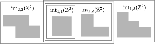
Figure 1:

We now extend the definition of erosion distance in [42]:

Definition 5.3.

Let $\mathcal{I}\subset\mathrm{Int}(\mathbb{Z}^{2})$ be closed under thickenings, and $M,N:\mathbb{Z}^{2}\to\mathbf{vec}$. We say there is an $\epsilon$-erosion between $\mathrm{rk}_{M}^{\mathcal{I}}$ and $\mathrm{rk}_{N}^{\mathcal{I}}$ if for all $I\in\mathcal{I}$, we have:

$$\mathrm{rk}_{M}(I^{\epsilon})\leq\mathrm{rk}_{N}(I)\hskip 28.45274pt\mathrm{and}\hskip 28.45274pt\mathrm{rk}_{N}(I^{\epsilon})\leq\mathrm{rk}_{M}(I)$$

Define the erosion distance between $\mathrm{rk}_{M}^{\mathcal{I}}$ and $\mathrm{rk}_{N}^{\mathcal{I}}$ as:

$$d_{\mathrm{E}}(\mathrm{rk}_{M}^{\mathcal{I}},\mathrm{rk}_{N}^{\mathcal{I}}):=\inf\{\epsilon\geq 0\,|\,\exists\,\mathrm{an}\,\epsilon-\mathrm{erosion\ between\ }\mathrm{rk}_{M}^{\mathcal{I}}\,\mathrm{and}\,\mathrm{rk}_{N}^{\mathcal{I}}\},$$

and $d_{\mathrm{E}}(\mathrm{rk}_{M}^{\mathcal{I}},\mathrm{rk}_{N}^{\mathcal{I}}):=\infty$ if no such erosion exists.

Theorem 5.4.

Let $\mathcal{I}\subset\mathrm{Int}(\mathbb{Z}^{2})$ be closed under thickenings, and $M,N:\mathbb{Z}^{2}\to\mathbf{vec}$. Then:

$$d_{\mathrm{E}}(\mathrm{rk}_{M}^{\mathcal{I}}),\mathrm{rk}_{N}^{\mathcal{I}})\leq d_{\mathrm{I}}(M,N).$$ (5.1)

For the proof of Theorem 5.4, we make use of the following well-known concrete formulation of the limit and colimit of any $M:\mathrm{P}\to\mathbf{vec}$ (see e.g. [29]):

Convention 5.5.

1. The limit of $M$ is the pair $(W,(\pi_{p})_{p\in\mathrm{P}})$ described as:

   $$W:=\left\{(\ell_{p})_{p\in\mathrm{P}}\in\prod_{p\in\mathrm{P}}M_{p}:\ \forall p\leq q\in\mathrm{P},\varphi_{M}(p,q)(\ell_{p})=\ell_{q}\right\}$$

   and for each $p\in\mathrm{P}$, the map $\pi_{p}:W\rightarrow M_{p}$ is the canonical projection. An element of $W$ is called a section of $M$.

2. The colimit of $M$ is isomorphic to a pair $(C,(i_{k})_{k\in\mathrm{P}})$. For $k\in\mathrm{P}$, let $\bar{i}_{k}:M_{k}\to\oplus_{k\in\mathrm{P}}M_{k}$ be the canonical injection. $C$ is the quotient space $\left(\oplus_{k\in\mathrm{P}}M_{k}\right)/V$, where $V$ is generated by $\bar{i}_{k}(v_{k})-\bar{i}_{\ell}(v_{\ell})$ over all $k\leq\ell$ in $\mathrm{P}$, with $v_{k}\in M_{k},v_{\ell}\in M_{\ell}$. Letting $q$ be the quotient map from $\oplus_{k\in\mathrm{P}}M_{k}$ to $C$, for $k\in\mathrm{P}$, $i_{k}:M_{k}\to C$ is the composition $q\circ\bar{i}_{k}$.

Proof of Theorem 5.4.

If $d_{\mathrm{I}}(M,N)=\infty$, there is nothing to prove. Let $\epsilon\geq 0$, and suppose that $\alpha:M\to N^{\vec{\epsilon}}$ and $\beta:N\to M^{\vec{\epsilon}}$ give an $\epsilon$-interleaving. Fix $I\in\mathcal{I}$. We show $\mathrm{rk}_{N}(I^{\epsilon})\leq\mathrm{rk}_{M}(I)$. Consider the diagram:

If $\alpha^{\prime},\beta^{\prime}$ exist which make this diagram commute, then the limit-to-colimit map on $N|_{I^{\epsilon}}$ factors through the limit-to-colimit map on $M|_{I}$, implying the desired bound.

Define $\alpha^{\prime}$ by $(\ell_{p})_{p\in I^{\epsilon}}\mapsto(\alpha_{p}(\ell_{p}))_{p+\overline{\epsilon}\in I}$. This $(\alpha_{p}(\ell_{p}))_{p+\overline{\epsilon}\in I}$ is a section of $M|_{I}$ by naturality of $\alpha$ and the fact that if $p+\vec{\epsilon}\in I$ then $p\in I^{\epsilon}$. Define $\beta^{\prime}$ by $[v_{p}]\mapsto[\beta_{p}(v_{p})]$ for any $p\in I$ and $v_{p}\in M_{p}$. By naturality of $\beta$, and since $p+\overline{\epsilon}\in I^{\epsilon}$, $\beta^{\prime}$ is well-defined.

Fix any $p_{0}\in I$. Then both $p_{0}+\vec{\epsilon},p_{0}-\vec{\epsilon}\in I^{\epsilon}$. We follow any section $(\ell_{p})_{p\in I^{\epsilon}}$ in the previous diagram and observe commutativity:

Thus, $\mathrm{rk}_{N}(I^{\epsilon})\leq\mathrm{rk}_{M}(I)$ and a symmetric argument gives $\mathrm{rk}_{M}(I^{\epsilon})\leq\mathrm{rk}_{N}(I^{\epsilon})$, so
$d_{E}(\mathrm{rk}_{M}^{\mathcal{I}},\mathrm{rk}_{N}^{\mathcal{I}})\leq\epsilon$, as desired. ∎

For example, let $\mathcal{I}:=\mathrm{int}_{m,n}(\mathbb{Z}^{2})$ (cf. Example 5.2). In light of Theorem 4.1, the discriminating power of the LHS in equation (5.1) is increasing as $m,n$ increase.

Remark 5.6 (Complexity of the erosion distance).

The computation of $d_{\mathrm{E}}$ between the RI’s of $[n]^{3}$-modules was implemented in [19]. The implementation therein can be modified easily to compute $d_{\mathrm{E}}$ between the RI’s of $[n]^{d}$-modules, in time $O(n^{2d}\log n)$ [30, Section 5]. On the other hand, $d_{\mathrm{I}}$ between $\mathbb{Z}^{d}$-modules is NP-hard to compute for $d>1$ [5].

6 Generalized Rank Invariant versus Zigzag-path-indexed barcode

In this section, we focus on $\mathbb{Z}^{2}$-modules and their GRIs over finite subsets of $\mathbb{Z}^{2}$. We use $\mathrm{int}(\mathbb{Z}^{2})$ and $\mathrm{con}(\mathbb{Z}^{2})$ to refer to finite intervals and finite connected subposets of $\mathbb{Z}^{2}$, respectively. We then use the term $\mathrm{int}$-GRI to refer to the GRI over $\mathrm{int}(\mathbb{Z}^{2})$.

In Section 6.1, we show that the ZIB over simple paths and the $\mathrm{int}$-GRI do not determine each other. As a corollary to this result and [24, Theorem 24], it follows that the ZIB over all paths is a strictly finer invariant than both the ZIB over simple paths and the $\mathrm{int}$-GRI: see Examples 6.3, 6.4 and Figure 2. In Section 6.2, using Möbius inversion, we show that the ZIB over simple paths and the Int-GRI approximate each other: see Remark 6.6 and Proposition 6.8. In Section 6.3, we provide a stability result for ZIBs: see Theorem 6.9.

6.1 ZIB over simple paths and the int-GRI are not equivalent

By a path (in $\mathbb{Z}^{2}$), we mean a nonempty finite sequence $\Gamma:p_{1},p_{2},\ldots,p_{n}$ in $\mathbb{Z}^{2}$ such that $p_{i}\triangleleft p_{i+1}$ or $p_{i+1}\triangleleft p_{i}$ for each $i=1,\ldots n-1$. Given another path $\Gamma^{\prime}$, we write $\Gamma^{\prime}\leq\Gamma$ if $\Gamma^{\prime}$ is a subpath of $\Gamma$, i.e. $\Gamma^{\prime}$ is $p_{a},p_{a+1},\ldots,p_{b}$ for some $1\leq a\leq b\leq n$. The path $\Gamma$ is called simple if all of $p_{1},p_{2},\ldots,p_{n}$ are distinct from each other. There are two special types of simple paths: We call $\Gamma$ a monotone path or positive path, if $p_{i}\triangleleft p_{i+1}$ for each $i=1,\ldots n-1$. We call $\Gamma$ a negative path if $\Gamma$ is obtained from the reflection of a monotone path with respect to the $y$-axis.

Note that the set $\{p_{1},\ldots,p_{n}\}$ of points in $\Gamma$ inherits the order of $\mathbb{Z}^{2}$, forming the zigzag poset $p_{1}\leftrightarrow p_{2}\leftrightarrow\cdots\leftrightarrow p_{n}$, where $\leftrightarrow$ stands for either $\leq$ or $\geq$. Let $M$ be a $\mathbb{Z}^{2}$-module. We denote the restriction of $M$ to the path $\Gamma$ by $M_{\Gamma}$, which is a zigzag module.

The map sending each positive path $\Gamma$ to $\mathrm{barc}(M_{\Gamma})$ amounts to the RI of $M$ [16]. In this light, we consider two invariants of $M$, both of which refine the RI of $M$.

Definition 6.1.

Let $\mathbb{ZZ}$ be the collection of all finite paths in $\mathbb{Z}^{2}$ and let $\mathrm{S}\mathbb{ZZ}$ be the collection of all finite simple paths in $\mathbb{Z}^{2}$. We define the zigzag-path-indexed barcode (ZIB) $M_{\mathbb{ZZ}}$ of $M$ as the map sending each $\Gamma\in\mathbb{ZZ}$ to $\mathrm{barc}(M_{\Gamma})$. The restriction of $M_{\mathbb{ZZ}}$ to $\mathrm{S}\mathbb{ZZ}$ is called the ZIB over simple paths, denoted by $M_{\mathrm{S}\mathbb{ZZ}}$.

Let $A$ and $B$ be two invariants of $\mathbb{Z}^{2}$-modules. If $A$ determines $B$, then we write $A\Rightarrow B$, which defines a transitive relation on the class of invariants of $\mathbb{Z}^{2}$-modules. For example, ZIB $\Rightarrow$ ZIB over simple paths. (but, we do not know a priori whether ZIB over simple paths determines ZIB). If $A$ determines $B$ and vice versa, then we write $A\Leftrightarrow B$. For example, we have $\mathrm{\mathrm{dgm}}_{M}\Leftrightarrow\mathrm{rk}_{M}$, by definition of $\mathrm{\mathrm{dgm}}_{M}$.

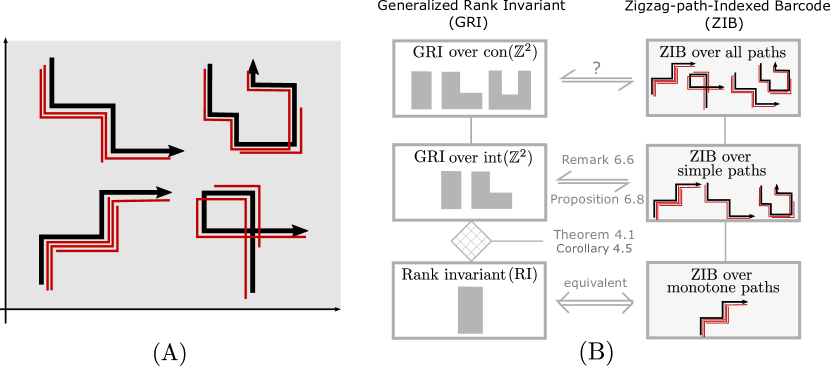
Figure 2: (A) Barcodes of a $\mathbb{Z}^{2}$-module over zigzag paths. (B) Hierarchy of invariants for $\mathbb{Z}^{2}$-modules. The hierarchy of the GRI (left column) is comparable to the hierarchy of barcodes over zigzag paths (right column). An invariant A is strictly finer than another invariant B at a lower height, i.e. A uniquely determines B, but not the other way. See Remark 6.2 for a full explanation.

Remark 6.2 (Interpretation of Figure 2).

1. Clearly, $A\Rightarrow B$ if $A$ and $B$ are in the same column, and $A$ is at a higher level than $B$.

2. (GRI over $\mathrm{con}(\mathbb{Z}^{2})$ $\Rightarrow$ ZIB over simple paths) follows from the definition of GRI over $\mathrm{con}(\mathrm{P})$.

3. (RI $\Leftrightarrow$ ZIB over monotone paths) was noted in [16, 35].

4. (ZIB over all paths $\Rightarrow$ GRI over $\mathrm{int}(\mathbb{Z}^{2})$) is a direct corollary of [24, Theorem 24].

5. Theorem 4.1 and Corollary 4.5 provide a faithful interpolation between the $\mathrm{int}$-GRI and RI of $\mathbb{Z}^{2}$-modules. (note, however, that Theorem 4.1 and Corollary 4.5 claim much more general statements than this interpolation since they consider $\mathrm{P}$-modules not just $\mathbb{Z}^{2}$-modules.)

6. Overall, by transitivity of $\Rightarrow$, it follows that ($A\Rightarrow B$) if $A$ is at a higher level than $B$ regardless of the columns they belong to.

In the following two examples, we will see that ($\mathrm{int}$-GRI$\not\Rightarrow$ZIB over simple paths) and (ZIB over simple paths $\not\Rightarrow$ $\mathrm{int}$-GRI).

Example 6.3 ($\mathrm{int}$-GRI$\not\Rightarrow$ZIB over simple paths).

Let $M,N$ be $\mathbb{Z}^{2}$-modules defined as below whose supports are contained in $[3]^{2}\subset\mathbb{Z}^{2}$. Also, let $\Gamma:(1,2),(1,3),(2,3),(3,3),(3,2),$ $(3,1),(2,1)$ (cf. Figure 3 (C)). It is not difficult to check that $M_{\Gamma}\not\cong N_{\Gamma}$, whereas $\mathrm{rk}_{M}(I)=\mathrm{rk}_{N}(I)$ for all $I\in\mathrm{Int}([3]^{2})$ [31, Example A.2]. This shows that the GRI over $\mathrm{int}(\mathbb{Z}^{2})$ cannot fully recover the ZIB over simple paths, the ZIB over all paths, nor the GRI over $\mathrm{con}(\mathbb{Z}^{2})$.

$$M:=\leavevmode\hbox to94.14pt{\vbox to80.7pt{\text{[drawing]}}}\oplus\leavevmode\hbox to90.4pt{\vbox to78.89pt{\text{[drawing]}}} {k} {k} {k} {k} {k^{2}} {k} {0} {k} {k} \scriptstyle{1} \scriptstyle{1} \scriptstyle{1} \scriptstyle{\begin{bmatrix}0\\ 1\end{bmatrix}} \scriptstyle{\begin{bmatrix}0\ 1\end{bmatrix}} \scriptstyle{\begin{bmatrix}0\ 1\end{bmatrix}} \scriptstyle{1} \scriptstyle{\begin{bmatrix}1\\ 1\end{bmatrix}} \scriptstyle{1} \scriptstyle{1} {k} {k} {k} {0} {k} {k} {0} {0} {k} \scriptstyle{1} \scriptstyle{1} \scriptstyle{1} \scriptstyle{1} \scriptstyle{1} \scriptstyle{1} {k} {k} {k} {k} {k^{2}} {k} {0} {k} {k} \scriptstyle{1} \scriptstyle{1} \scriptstyle{1} \scriptstyle{\begin{bmatrix}0\\ 1\end{bmatrix}} \scriptstyle{\begin{bmatrix}0\ 1\end{bmatrix}} \scriptstyle{\begin{bmatrix}0\ 1\end{bmatrix}} \scriptstyle{1} \scriptstyle{\begin{bmatrix}1\\ 1\end{bmatrix}} \scriptstyle{1} \scriptstyle{1} {k} {k} {k} {0} {k} {k} {0} {0} {k} \scriptstyle{1} \scriptstyle{1} \scriptstyle{1} \scriptstyle{1} \scriptstyle{1} \scriptstyle{1}$$

$$N:=\leavevmode\hbox to91.34pt{\vbox to78.89pt{\text{[drawing]}}}\oplus\leavevmode\hbox to90.4pt{\vbox to78.89pt{\text{[drawing]}}}\oplus\leavevmode\hbox to89.35pt{\vbox to77.89pt{\text{[drawing]}}} {k} {k} {k} {k} {k} {k} {0} {0} {k} \scriptstyle{1} \scriptstyle{1} \scriptstyle{1} \scriptstyle{1} \scriptstyle{1} \scriptstyle{1} \scriptstyle{1} \scriptstyle{1} {k} {k} {k} {0} {k} {k} {0} {k} {k} \scriptstyle{1} \scriptstyle{1} \scriptstyle{1} \scriptstyle{1} \scriptstyle{1} \scriptstyle{1} \scriptstyle{1} \scriptstyle{1} {0} {0} {0} {0} {k} {0} {0} {0} {0} {k} {k} {k} {k} {k} {k} {0} {0} {k} \scriptstyle{1} \scriptstyle{1} \scriptstyle{1} \scriptstyle{1} \scriptstyle{1} \scriptstyle{1} \scriptstyle{1} \scriptstyle{1} {k} {k} {k} {0} {k} {k} {0} {k} {k} \scriptstyle{1} \scriptstyle{1} \scriptstyle{1} \scriptstyle{1} \scriptstyle{1} \scriptstyle{1} \scriptstyle{1} \scriptstyle{1} {0} {0} {0} {0} {k} {0} {0} {0} {0}$$

Example 6.4 (ZIB over simple paths $\not\Rightarrow$ $\mathrm{int}$-GRI).

Let $I\in\mathrm{int}(\mathbb{Z}^{2})$ with the following directed Hasse diagram.

$$I:=\leavevmode\hbox to126.44pt{\vbox to41.63pt{\text{[drawing]}}} {\bullet} {\bullet} {\bullet} {\bullet} {\bullet} {\bullet} {\bullet} {\bullet} {\bullet} {\bullet} {\bullet} {\bullet}$$

Let us define $\mathbb{Z}^{2}$-modules $M,N$ supported on $I$ as follows.

$$M:=k_{I}\oplus\leavevmode\hbox to134.13pt{\vbox to68.86pt{\text{[drawing]}}} {k} {k^{2}} {k} {k} {k^{2}} {k} \scriptstyle{\begin{bmatrix}1\\ 0\end{bmatrix}} \scriptstyle{\begin{bmatrix}1\ 1\end{bmatrix}} \scriptstyle{\begin{bmatrix}0\\ 1\end{bmatrix}} \scriptstyle{\begin{bmatrix}1\\ 1\end{bmatrix}} \scriptstyle{\begin{bmatrix}0\ 1\end{bmatrix}} \scriptstyle{\begin{bmatrix}1\ 0\end{bmatrix}} {k} {k^{2}} {k} {k} {k^{2}} {k} \scriptstyle{\begin{bmatrix}1\\ 0\end{bmatrix}} \scriptstyle{\begin{bmatrix}1\ 1\end{bmatrix}} \scriptstyle{\begin{bmatrix}0\\ 1\end{bmatrix}} \scriptstyle{\begin{bmatrix}1\\ 1\end{bmatrix}} \scriptstyle{\begin{bmatrix}0\ 1\end{bmatrix}} \scriptstyle{\begin{bmatrix}1\ 0\end{bmatrix}}$$

$$N:=\leavevmode\hbox to131.33pt{\vbox to59.02pt{\text{[drawing]}}}\hskip 14.22636pt\oplus\leavevmode\hbox to131.33pt{\vbox to63.23pt{\text{[drawing]}}} {k} {k^{2}} {k} {k} {k} {k} \scriptstyle{\begin{bmatrix}1\\ 0\end{bmatrix}} \scriptstyle{\begin{bmatrix}1\ 1\end{bmatrix}} \scriptstyle{\begin{bmatrix}0\\ 1\end{bmatrix}} \scriptstyle{\mathrm{id}} \scriptstyle{\mathrm{id}} \scriptstyle{\mathrm{id}} {k} {k} {k} {k} {k^{2}} {k} \scriptstyle{\mathrm{id}} \scriptstyle{\mathrm{id}} \scriptstyle{\mathrm{id}} \scriptstyle{\begin{bmatrix}1\\ 1\end{bmatrix}} \scriptstyle{\begin{bmatrix}0\ 1\end{bmatrix}} \scriptstyle{\begin{bmatrix}1\ 0\end{bmatrix}} {k} {k^{2}} {k} {k} {k} {k} \scriptstyle{\begin{bmatrix}1\\ 0\end{bmatrix}} \scriptstyle{\begin{bmatrix}1\ 1\end{bmatrix}} \scriptstyle{\begin{bmatrix}0\\ 1\end{bmatrix}} \scriptstyle{\mathrm{id}} \scriptstyle{\mathrm{id}} \scriptstyle{\mathrm{id}} {k} {k} {k} {k} {k^{2}} {k} \scriptstyle{\mathrm{id}} \scriptstyle{\mathrm{id}} \scriptstyle{\mathrm{id}} \scriptstyle{\begin{bmatrix}1\\ 1\end{bmatrix}} \scriptstyle{\begin{bmatrix}0\ 1\end{bmatrix}} \scriptstyle{\begin{bmatrix}1\ 0\end{bmatrix}}$$

Since each summand of $M$ and $N$ is indecomposable, by Theorem 2.14, we have $\mathrm{rk}_{M}(I)=1$ and $\mathrm{rk}_{N}(I)=0$. Now we claim that $M_{\mathrm{S}\mathbb{ZZ}}=N_{\mathrm{S}\mathbb{ZZ}}$. Since $M$ and $N$ are supported on $I$, it suffices to show $M_{\Gamma}\cong N_{\Gamma}$ for all maximal simple paths $\Gamma$ in $I$. Indeed, it is not difficult to check that $M_{\Gamma}\cong N_{\Gamma}$ for all of the six maximal simple paths $\Gamma$ in $I$:

Therefore, the ZIB over simple paths cannot fully recover the GRI over $\mathrm{int}(\mathbb{Z}^{2})$ in general.

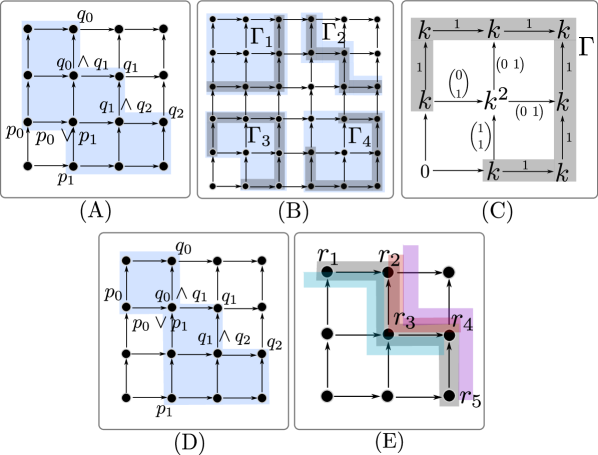
Figure 3: (A) An interval $I$ in $\mathbb{Z}^{2}$ with labels for points in $\min_{\mathbb{ZZ}}(I)$ and $\max_{\mathbb{ZZ}}(I)$. (B) Paths $\Gamma_{i}$ for $i=1,2,3,4$ in $\mathbb{Z}^{2}$ (directions are not specified) and their interval-hulls. Whereas $\Gamma_{i}$ is a tame path for $i=1,2,4$, the path $\Gamma_{3}$ is not a tame path. (C) An example showing that the rank over the non-tame path $\Gamma$ does not coincide with the rank over the interval-hull $I_{\Gamma}$. (D) An interval in $\mathbb{Z}^{2}$ which is not solid nor thin. The interval in (A) is solid. The interval $I_{\Gamma_{2}}$ in (B) is thin. (E) Let $\Gamma$ be the path $r_{1},\ldots,r_{5}$ and $\Gamma^{\prime}$ be the subpath $r_{2},r_{3},r_{4}$. Then $\Gamma^{\prime-}$, $\Gamma^{\prime+}$, $\Gamma^{\prime\pm}$ are the paths $r_{1},r_{2},r_{3},r_{4}$ and $r_{2},r_{3},r_{4},r_{5}$ and $r_{1},r_{2},r_{3},r_{4},r_{5}$, respectively.

6.2 ZIB over simple paths and the int-GRI approximate each other

Although the GRI over $\mathrm{int}(\mathbb{Z}^{2})$ and $(-)_{\mathrm{S}\mathbb{ZZ}}$ fail to determine each other, we can estimate one from the other. In this section, we clarify how: Remark 6.6 and Proposition 6.8.

Let $I_{\Gamma}$ be the smallest interval of $\mathbb{Z}^{2}$ that contains $\Gamma$, i.e. $I_{\Gamma}:=\{q\in\mathbb{Z}^{2}:\exists p,r\in\Gamma,\ \ p\leq q\leq r\}$. We call $I_{\Gamma}$ the interval-hull of $\Gamma$. See Figure 3 (B) for illustrative examples.

Next we introduce the notion of tame path, a generalization of the boundary cap introduced in [24] as a bridge between the GRI of $\mathbb{Z}^{2}$-modules and zigzag modules. Let $I\in\mathrm{int}(\mathbb{Z}^{2})$. Note that $\min(I)$ and $\max(I)$ respectively form antichains in $I$, i.e. any two different points in $\min(I)$ (or in $\max(I)$) are not comparable. Since $\min(I)$ is a finite antichain, we can list the elements of $\min(I)$ in ascending order of their $x$-coordinates, i.e. $\min(I):=\{p_{0},\ldots,p_{k}\}$ and such that for each $i=0,\ldots,k,$ the $x$-coordinate of $p_{i}$ is less than that of $p_{i+1}$. Similarly, let $\max(I):=\{q_{0},\ldots,q_{\ell}\}$ be ordered in ascending order of $q_{j}$’s $x$-coordinates. We have that $p_{0}\leq q_{0}$ (cf. Figure 3 (A)). We define the following two paths.

$$\min_{\mathbb{ZZ}}(I) :p_{0}<(p_{0}\vee p_{1})>p_{1}<(p_{1}\vee p_{2})>\cdots<(p_{k-1}\vee p_{k})>p_{k}$$

$$\max_{\mathbb{ZZ}}(I) :q_{0}>(q_{0}\wedge q_{1})<q_{1}>(q_{1}\wedge q_{2})<\cdots>(q_{\ell-1}\wedge q_{\ell})>q_{\ell}$$ (6.1)

We call a path $\Gamma$ in $\mathbb{Z}^{2}$ a tame if [$\min_{\mathbb{ZZ}}(I_{\Gamma})\leq\Gamma$ or $\min_{\mathbb{ZZ}}(I_{\Gamma})^{-1}\leq\Gamma$] and [$\max_{\mathbb{ZZ}}(I_{\Gamma})\leq\Gamma$ or $\max_{\mathbb{ZZ}}(I_{\Gamma})^{-1}\leq\Gamma$]. For example, in Figure 3 (B), $\Gamma_{1}$, $\Gamma_{2}$, and $\Gamma_{4}$ are tame but $\Gamma_{3}$ is not.

Let us fix a $\mathbb{Z}^{2}$-module $M$. We obtain a slight extension of [24, Theorem 24]:

Proposition 6.5.

Given any tame path $\Gamma$ in $\mathbb{Z}^{2}$, $\mathrm{rk}(M_{\Gamma})=\mathrm{rk}_{M}({I_{\Gamma}})$.

The proof of Proposition 6.5 similar to that of [24, Theorem 24] and thus we defer it to the appendix.

An $I\in\mathrm{int}(\mathbb{Z}^{2})$ is called solid if $\min_{\mathbb{ZZ}}(I)$ and $\max_{\mathbb{ZZ}}(I)$ do not intersect. For example, the interval given in Figure 3 (A) is solid. On the contrary, if $I$ equals $I_{\Gamma}$ for some negative path $\Gamma$, then $I$ is called thin.

Remark 6.6 (Approximating the $\mathrm{int}$-GRI over $\mathrm{int}(\mathbb{Z}^{2})$ via the ZIB over simple paths).

Let $I\in\mathrm{int}(\mathbb{Z}^{2})$.

1. If $I$ is a thin interval, then $I$ is covered by a simple path $\Gamma$ and thus $\mathrm{rk}_{M}(I)$ equals the multiplicity of the full bar in $\mathrm{barc}(M_{\Gamma})$ by Theorem 2.14.

2. If $I$ is solid, then there exists a simple tame path $\Gamma$ such that $I=I_{\Gamma}$ [24, Definition 19]. Hence $\mathrm{rk}_{M}(I)$ is the multiplicity of the full bar in $\mathrm{barc}(M_{\Gamma})$ by Theorem 2.14.

3. If $I$ is not solid nor thin, then it is not difficult to observe that no simple tame path spans $I$. However, by monotonicity of the GRI (Remark 2.15 (i)), we have the following upper and lower bounds for $\mathrm{rk}_{M}(I)$, which can be obtained from the ZIB.

   $$\max_{J}\mathrm{rk}_{M}(J)\leq\mathrm{rk}_{M}(I)\leq\min_{\Gamma}\mathrm{rk}_{M}(\Gamma)$$

   where the minimum is taken over all simple paths $\Gamma$ in $I$ and the maximum is taken over all solid intervals $J\supset I$. It is clear that $\max_{\Gamma}\mathrm{rk}_{M}(\Gamma)$ is subsumed by $M_{\mathrm{S}\mathbb{ZZ}}$. From item (ii), $\min_{J}\mathrm{rk}_{M}(J)$ is also subsumed by $M_{\mathrm{S}\mathbb{ZZ}}$.

Next, we approximate $M_{\mathrm{S}\mathbb{ZZ}}$ via $\mathrm{rk}_{M}$ on $\mathrm{int}(\mathbb{Z}^{2})$. Let $m_{\Gamma}:=\mathrm{rk}_{M}(I_{\Gamma})$ and $\ell_{\Gamma}:=\min\{\mathrm{rk}(M_{\Gamma^{\prime}}):\Gamma^{\prime}\leq\Gamma,\ \mbox{$\Gamma^{\prime}$ is tame}\}.$ Then, by monotonicity of $\mathrm{rk}_{M}$ (Remark 2.15 (i)), we have:

$$m_{\Gamma}\leq\mathrm{rk}(M_{\Gamma})\leq\ell_{\Gamma}.$$ (6.2)

Remark 6.7.

1. By Proposition 6.5, the GRI over $\mathrm{int}(\mathbb{Z}^{2})$ subsumes $m_{\Gamma}$ and $\ell_{\Gamma}$.

2. Again by Proposition 6.5, if $\Gamma$ is tame, then $m_{\Gamma}=\ell_{\Gamma}=\mathrm{rk}(M_{\Gamma})$.

Let $\Gamma:r_{1},r_{2},\ldots,r_{n}$ be a path and let $\Gamma^{\prime}:r_{k},r_{k+1},\ldots,r_{\ell}$ be a subpath of $\Gamma$. When $k\neq 1$, we consider the one-point extension $\Gamma^{\prime-}$ of $\Gamma^{\prime}$ to the left, i.e. $\Gamma^{\prime-}:r_{k-1},r_{k},\ldots,r_{\ell}$. When $\ell\neq n$, we consider the one-point extension $\Gamma^{\prime+}$ of $\Gamma^{\prime}$ to the right, i.e. $\Gamma^{\prime+}:r_{k},\ldots,r_{\ell},r_{\ell+1}$. When $k\neq 1$ and $\ell\neq n$, we consider the two-point extension $\Gamma^{\prime\pm}:r_{k-1},r_{k},\ldots,r_{\ell},r_{\ell+1}$ of $\Gamma^{\prime}$ within $\Gamma$ (see Figure 3 (E) for an illustrative example).

By utilizing Proposition 6.5, we obtain certain upper and lower bounds on the multiplicity of each subpath $\Gamma^{\prime}$ of $\Gamma$ in $\mathrm{barc}(M_{\Gamma})$ in Proposition 6.8 below. By Remark 6.7 (ii), those two bounds match when $\Gamma^{\prime\pm}\leq\Gamma$ and $\Gamma$ is either a monotone path or a negative path (and thus tame).

Proposition 6.8 (Approximating the ZIB over simple paths via the $\mathrm{int}$-GRI).

Let $n_{\Gamma^{\prime}}$ be the multiplicity of $\Gamma^{\prime}$ in $\mathrm{barc}(M_{\Gamma})$. Then, we have

$$m_{\Gamma^{\prime}}-\ell_{\Gamma^{\prime+}}-\ell_{\Gamma^{\prime-}}+m_{\Gamma^{\prime\pm}}\leq n_{\Gamma^{\prime}}\leq\ell_{\Gamma^{\prime}}-m_{\Gamma^{\prime+}}-m_{\Gamma^{\prime-}}+\ell_{\Gamma^{\prime\pm}}.$$ (6.3)

Proof.

By the principle of inclusion and exclusion, we have that

$$n_{\Gamma^{\prime}}=\mathrm{rk}(M_{\Gamma^{\prime}})-\mathrm{rk}(M_{\Gamma^{\prime+}})-\mathrm{rk}(M_{\Gamma^{\prime-}})+\mathrm{rk}(M_{\Gamma^{\prime\pm}})\ \ \ \mbox{(cf. \cite[cite]{[\@@bibref{}{kim2021generalized}{}{}, Section 3]}).}$$ (6.4)

From the inequalities in (6.2), the claimed inequalities directly follow. ∎

6.3 Stability of the (restricted) ZIBs

In this section, we reinterpret Theorem 5.4 in terms of (restricted) ZIBs. Let $\mathcal{I}$ be any subset of $\mathrm{int}(\mathbb{Z}^{2})$ closed under thickenings and let $\mathbb{ZZ}_{\mathcal{I}}:=\{\Gamma\in\mathbb{ZZ}:I_{\Gamma}\in\mathcal{I}\}.$ For each $\Gamma$ and $\epsilon\geq 0$, let $\Gamma^{\epsilon}$ be any path such that $I_{\Gamma^{\epsilon}}=I^{\epsilon}$ (such path always exists [24, Definition 19]). Given any $\mathbb{Z}^{2}$-module $M$, by Proposition 6.5, $\mathrm{rk}(M_{\Gamma^{\epsilon}})=\mathrm{rk}_{M}(I^{\epsilon})$. Let $M_{\mathbb{ZZ}_{\mathcal{I}}}$ be the ZIB of $M$ over paths in $\mathbb{ZZ}_{\mathcal{I}}$, i.e. the map sending each $\Gamma\in\mathbb{ZZ}_{\mathcal{I}}$ to $\mathrm{barc}(M_{\Gamma})$. Given another $\mathbb{Z}^{2}$-module $N$, we define the erosion distance $d_{\mathrm{E}}(M_{\mathbb{ZZ}_{\mathcal{I}}},N_{\mathbb{ZZ}_{\mathcal{I}}})$ as the infimum $\epsilon\geq 0$ for which for any $\Gamma\in\mathbb{ZZ}_{\mathcal{I}}$, we have $\mathrm{rk}(M_{\Gamma^{\epsilon}})\leq\mathrm{rk}(N_{\Gamma})$ and $\mathrm{rk}(M_{{\Gamma}^{\epsilon}})\leq\mathrm{rk}(N_{\Gamma})$. In the light of Theorems 2.2, 2.14 and Proposition 6.5, the condition $\mathrm{rk}(M_{\Gamma^{\epsilon}})\leq\mathrm{rk}(N_{\Gamma})$ can be read as (The multiplicity of the full bar in $\mathrm{barc}(M_{\Gamma^{\epsilon}})$) $\leq$ (The multiplicity of the full bar in $\mathrm{barc}(N_{\Gamma})$).

Theorem 6.9 (Reinterpretation of Theorem 5.4).

Let $\mathcal{I}\subset\mathrm{int}(\mathbb{Z}^{2})$ be any collection of intervals closed under thickenings. Then for any $\mathbb{Z}^{2}$-modules $M$ and $N$:

$$d_{\mathrm{E}}(M_{\mathbb{ZZ}_{\mathcal{I}}},N_{\mathbb{ZZ}_{\mathcal{I}}})\leq d_{\mathrm{I}}(M,N).$$

7 Discussion

A few open questions are as follows. (1) There is a recent algorithm developed by Dey and Hou for updating zigzag persistence [22] extending the vineyards algorithm [20] which can be utilized to compute the RI of an $[n]^{2}$-module in $O(n^{4})$ time [40]. This is more efficient than computing the RI by brute force, i.e. one-at-a-time for all $[p,q]\in\mathrm{Seg}(\mathrm{P})$. We wonder whether the zigzag persistence update algorithm can be used to compute the GRI over certain collections $\mathcal{I}$ (e.g. $\mathrm{int}_{m,n}(\mathbb{Z}^{2})$ in Example 5.2 or the collection in equation (3.4)) in a manner more efficient than the brute-force approach of computing $\mathrm{rk}_{\ast}(I)$ for all $I\in\mathcal{I}$. Similarly, such an approach, if possible, may provide for efficient computation of the ZIB.

(2) What is the relationship between the GRI over $\mathrm{con}(\mathbb{Z}^{2})$ and the ZIB over all paths? (cf. The top row in Figure 2)?

Acknowledgements.

This research was partially supported by the NSF through grants DMS-1723003, IIS-1901360, CCF-1740761, DMS-1547357 and by the BSF under grant 2020124. The authors thank anonymous reviewers for sharing their insight.

Appendix A Stability of restricted Generalized Rank Invariants over General Posets

We consider stability in the case where $\mathrm{P}$ is a more general poset. We compare $\mathrm{P}$-modules using the notion of interleaving distance on general persistence modules developed by Bubenik et al. in [12] and expanded upon by de Silva et al. in [21]. We review key definitions from these texts:

Definition A.1.

A translation on $\mathrm{P}$ is an endofunctor $\Gamma:\mathrm{P}\to\mathrm{P}$, together with a natural transformation $\eta:I_{\mathrm{P}}\to\Gamma$, where $I_{\mathrm{P}}$ is the identify functor.

We care about translations respecting the order of $\mathrm{P}$. For $\Gamma_{1},\Gamma_{2}:\mathrm{P}\to\mathrm{P}$, we say $\Gamma_{1}\leq\Gamma_{2}$ if for all $p\leq q\in\mathrm{P}$, $\Gamma_{1}(\mathrm{P})\leq\Gamma_{2}(q)$. A superlinear family of translations $\Omega$, is a family of translations $\Omega_{\epsilon}$ on $\mathrm{P}$, for $\epsilon\geq 0$, such that $I_{\mathrm{P}}=\Omega_{0}$, and $\Omega_{\epsilon}\Omega_{\zeta}\leq\Omega_{\epsilon+\zeta}$.

Throughout the following, $\Omega$ will refer to a family of superlinear translations on $\mathrm{P}$. For $\Omega_{\epsilon}$ a superlinear translation on $\mathrm{P}$ and $I\subset\mathrm{P}$, we denote $\Omega_{\epsilon}(I):=\{\Omega_{\epsilon}(\mathrm{P})\ |\ p\in I\}$. For all $\epsilon\geq 0$, the translation $\Omega_{\epsilon}$ comes with a natural transformation $\eta_{\epsilon}:I_{\mathrm{P}}\to\Omega_{\epsilon}$. For any $M:\mathrm{P}\to\mathbf{vec}$, this induces a natural transformation $M\eta_{\epsilon}:M\to M\Omega_{\epsilon}$. This is used to define:

Definition A.2.

Two $\mathrm{P}$-modules $M$ and $N$ are $\Omega_{\epsilon}$-interleaved if there exist a pair of natural transformations $\varphi:M\to N\Omega_{\epsilon}$ and $\psi:N\to M\Omega_{\epsilon}$ such that the diagram:

commutes. The pair $(\varphi,\psi)$ is an $\Omega_{\epsilon}$-interleaving.

The interleaving distance with respect to $\Omega$ is:

$$d_{\mathrm{I}}^{\Omega}(M,N):=\inf\{\epsilon\geq 0\ |\ M,N\ \mathrm{are\ }\Omega_{\epsilon}-interleaved\}$$

or $d_{\mathrm{I}}^{\Omega}(M,N):=\infty$ if there is no $\epsilon$-interleaving for any $\epsilon\geq 0$.

For example, if we take $P=\mathbb{Z}^{n}$ with the standard product order, and $\Omega$ to be the family with $\Omega_{\epsilon}$ the translation by $(\lfloor\epsilon\rfloor,\lfloor\epsilon\rfloor,\ldots,\lfloor\epsilon\rfloor)\in\mathbb{Z}^{n}$, then $d_{\mathrm{I}}^{\Omega}$ is the classical notion of interleaving as used in Section 5. Hence, $d_{\mathrm{I}}^{\Omega}$ is an extension of the usual $d_{\mathrm{I}}$ from [34].

We now adapt the definition of erosion distance to the more general setting.

Definition A.3.

Let $I\subset\mathrm{P}$ be non-empty. For $\epsilon>0$, we call $I^{\epsilon}$ the $\epsilon$-thickening of $I$, defined as:

$$I^{\epsilon}:=\{r\in\mathrm{P}\ |\ \exists p,q\in I\ \mathrm{with}\ p\leq\Omega_{\epsilon}(r)\mathrm{\ and}\ r\leq\Omega_{\epsilon}(q)\}.$$

Clearly, $I\subset I^{\epsilon}$. For example, if $P=\mathbb{R}$, and $\Omega$ is the family with $\Omega_{\epsilon}$ the translation by $\epsilon$ for $\epsilon\geq 0$, then for an interval $I=[a,b]$, its $\epsilon$-thickening would be the interval $I^{\epsilon}=[a-\epsilon,b+\epsilon]$. Furthermore, the $\epsilon$-thickening of an interval is an interval:

Proposition A.4.

Let $I\in\mathrm{Int}(\mathrm{P})$. Then $I^{\epsilon}\in\mathrm{Int}(\mathrm{P})$ for all $\epsilon\geq 0$.

Proof.

Let $\epsilon\geq 0$. We need to show that $I^{\epsilon}$ is non-empty, convex, and connected.

Since $I(\neq\emptyset)\subset I^{\epsilon}$, we have that $I^{\epsilon}$ is non-empty. Suppose $a,b\in I^{\epsilon}$, and $a\leq c\leq b$. By definition, there exist $p_{a},q_{a},p_{b},q_{b}\in I$ such that $p_{a}\leq\Omega_{\epsilon}(a)$, $p_{b}\leq\Omega_{\epsilon}(b)$, $a\leq\Omega_{\epsilon}(q_{a})$, and $b\leq\Omega_{\epsilon}(q_{b})$. Then we have: $p_{a}\leq\Omega_{\epsilon}(a)\leq\Omega_{\epsilon}(c)$ and $c\leq b\leq\Omega_{\epsilon}(q_{b})$, and thus $c\in I^{\epsilon}$.

To see connectivity, suppose $p,q\in I^{\epsilon}$. Note that for all $r\in I$, $\Omega_{\epsilon}(r)\in I^{\epsilon}$, which can be seen by letting $p=q=r$ in Definition A.3. Thus, we can find $r_{p},r_{q}\in I$ with $p\leq\Omega_{\epsilon}(r_{p})$ and $q\leq\Omega_{\epsilon}(r_{q})$. As $r_{p},r_{q}\in I$, there is a chain $r_{p}=a_{0},a_{1},\ldots,a_{n}=r_{q}$ of sequentially comparable elements of $I$. Then $p\leq\Omega_{\epsilon}(r_{p})\geq r_{p}=a_{0},a_{1},\ldots,a_{n}=r_{q}\leq\Omega_{\epsilon}(r_{q})\geq q$ gives a chain of sequentially comparable elements of $I^{\epsilon}$, so $I^{\epsilon}$ is connected. ∎

If $\mathcal{I}\subset\mathrm{Int}(\mathrm{P})$ and for all $I\in\mathcal{I}$ and $\epsilon\geq 0$, $I^{\epsilon}\in\mathcal{I}$, then we say $\mathcal{I}$ is closed under $\Omega$-thickenings.

Example A.5.

If $P=\mathbb{R}^{2}$ with the usual product order, and $\Omega$ is the family with $\Omega_{\epsilon}$ the translation by $(\epsilon,\epsilon)$ for $\epsilon\geq 0$, then for a rectangle $I=[a,b]$, its $\epsilon$-thickening would be $I^{\epsilon}=[a-(\epsilon,\epsilon),b+(\epsilon,\epsilon)]$. This is still a rectangle, so the collection of rectangles in $\mathbb{R}^{2}$ is closed under $\Omega$-thickenings.

Now we define the erosion distance:

Definition A.6.

Let $\mathcal{I}\subset\mathrm{Int}(\mathrm{P})$ be closed under $\Omega$-thickenings, and let $M,N$ be $\mathrm{P}$-modules. We say there is an $\epsilon$-erosion between $\mathrm{rk}_{M}^{\mathcal{I}}$ and $\mathrm{rk}_{N}^{\mathcal{I}}$ if for all $I\in\mathcal{I}$, we have:

$$\mathrm{rk}_{M}(I^{\epsilon})\leq\mathrm{rk}_{N}(I)\hskip 14.22636pt\mathrm{and}\hskip 14.22636pt\mathrm{rk}_{N}(I^{\epsilon})\leq\mathrm{rk}_{M}(I).$$

Define the erosion distance between $\mathrm{rk}_{M}^{\mathcal{I}}$ and $\mathrm{rk}_{N}^{\mathcal{I}}$ as:

$$d_{E}^{\Omega}(\mathrm{rk}_{M}^{\mathcal{I}},\mathrm{rk}_{N}^{\mathcal{I}}):=\inf\{\epsilon\geq 0\ |\ \exists\ \mathrm{an\ }\epsilon-\mathrm{erosion\ between\ }\mathrm{rk}_{M}^{\mathcal{I}}\ \mathrm{and}\ \mathrm{rk}_{N}^{\mathcal{I}}\}$$

and $d_{E}^{\Omega}(\mathrm{rk}_{M}^{\mathcal{I}},\mathrm{rk}_{N}^{\mathcal{I}}):=\infty$ if no such erosion exists.

Proposition A.7.

Fix a collection $\mathcal{I}\subset\mathrm{Int}(\mathrm{P})$ that is closed under $\Omega$-thickenings. Then $d_{E}^{\Omega}$ is an extended pseudometric on the collection $\{\mathrm{rk}_{M}^{\mathcal{I}}\ |\ M:\mathrm{P}\to\mathbf{vec}\}$.

Proof.

Since $\Omega_{0}=I_{\mathrm{P}}$, it is immediate that $d_{E}^{\Omega}(\mathrm{rk}_{M}^{\mathcal{I}},\mathrm{rk}_{M}^{\mathcal{I}})=0$. Symmetry is immediate from the definition.

It remains to show the triangle inequality. Note that $\Omega_{\epsilon}\Omega_{\epsilon^{\prime}}\leq\Omega_{\epsilon+\epsilon^{\prime}}$. This implies $(I^{\epsilon})^{\epsilon^{\prime}}\subset I^{\epsilon+\epsilon^{\prime}}$. From this, if there is an $\epsilon$-erosion between $\mathrm{rk}_{M}^{\mathcal{I}}$ and $\mathrm{rk}_{N}^{\mathcal{I}}$, and an $\epsilon^{\prime}$-erosion between $\mathrm{rk}_{N}^{\mathcal{I}}$ and $\mathrm{rk}_{L}^{\mathcal{I}}$, then for all $I\in\mathcal{I}$:

$$\mathrm{rk}_{M}(I)\geq\mathrm{rk}_{N}(I^{\epsilon})\geq\mathrm{rk}_{L}((I^{\epsilon})^{\epsilon^{\prime}})\geq\mathrm{rk}_{L}(I^{\epsilon+\epsilon^{\prime}})$$

$$\mathrm{rk}_{L}(I)\geq\mathrm{rk}_{N}(I^{\epsilon^{\prime}})\geq\mathrm{rk}_{M}((I^{\epsilon^{\prime}})^{\epsilon})\geq\mathrm{rk}_{M}(I^{\epsilon^{\prime}+\epsilon}),$$

hence there is an $(\epsilon+\epsilon^{\prime})$-erosion between $\mathrm{rk}_{M}^{\mathcal{I}}$ and $\mathrm{rk}_{L}^{\mathcal{I}}$, as desired. ∎

For stability to hold, we require that for all $\epsilon\geq 0$, $\Omega_{\epsilon}:\mathrm{P}\to\mathrm{P}$ be surjective. If this property is satisfied, we say $\Omega$ is surjective. For example, if $\Omega$ is the aforementioned shift by $(\lfloor\epsilon\rfloor,\lfloor\epsilon\rfloor)$ in $\mathbb{Z}^{2}$, then $\Omega$ is surjective.

Theorem A.8.

Fix $\Omega$ be a superlinear family of translations on $\mathrm{P}$ such that $\Omega$ is surjective. Let $\mathcal{I}\subset\mathrm{Int}(\mathrm{P})$ be a collection of finite intervals closed under $\Omega$-thickenings. Then for any $\mathrm{P}$-modules $M$ and $N$:

$$d_{E}^{\Omega}(\mathrm{rk}_{M}^{\mathcal{I}},\mathrm{rk}_{N}^{\mathcal{I}})\leq d_{\mathrm{I}}^{\Omega}(M,N)$$ (A.1)

We omit the proof of Theorem A.8 as it follows the same steps as the proof of Theorem 5.4, under simple adjustments to the general setting such as replacing $p+\epsilon$ with $\Omega_{\epsilon}(p)$. Surjectivity comes in to play in that it guarantees the existence of an element $p_{0}^{\prime}\in I^{\epsilon}$ such that $\Omega_{\epsilon}(p_{0}^{\prime})=p_{0}$, where $p_{0}^{\prime}$ and $p_{0}$ play the role of $p_{0}-\vec{\epsilon}$ and $p_{0}$, respectively, as in the proof of Theorem 5.4.

Appendix B Section 6 materials

Proof of Proposition 6.5

To prove Proposition 6.5, we need the following definition and lemmas (which are also used in [24]). Recall the construction of the (co)limit from Convention 5.5.

Let $\mathrm{P}$ be a poset and let $M$ be any $\mathrm{P}$-module. Let $p,q\in\mathrm{P}$ and let $v_{p}\in M_{p}$ and $v_{q}\in M_{q}$. We write $v_{p}\sim v_{q}$ if $\mathrm{P}$ and $q$ are comparable, and either $v_{p}$ is mapped to $v_{q}$ via $\varphi_{M}(p,q)$ or $v_{q}$ is mapped to $v_{p}$ via $\varphi_{M}(q,p)$.

Definition B.1.

Let $\Gamma:p_{0},\ldots,p_{k}$ be a path in $\mathrm{P}$. A $(k+1)$-tuple $\mathbf{v}\in\bigoplus_{i=0}^{k}M_{p_{i}}$ is called the section of $M$ along $\Gamma$ if $\mathbf{v}_{p_{i}}\sim\mathbf{v}_{p_{i+1}}$ for each $i$.

Note that $\mathbf{v}$ is not necessarily a section of the restriction $M|_{\{p_{0},\ldots,p_{k}\}}$ of $M$ to the subposet $\{p_{0},\ldots,p_{k}\}\subset I$ [24, Example 21]. Furthermore, $\Gamma$ can contain multiple copies of the same point in $\mathrm{P}$.

Lemma B.2.

Let $p,q\in\mathrm{P}$. For any vectors $v_{p}\in M_{p}$ and $v_{q}\in M_{q}$, $[v_{p}]=[v_{q}]$ in the colimit $\varinjlim M$ if and only if there exist a path $\Gamma:p=p_{0},p_{1},\ldots,p_{n}=q$ in $\mathrm{P}$ and a section $\mathbf{v}$ of $M$ along $\Gamma$ such that $\mathbf{v}_{p}=v_{p}$ and $\mathbf{v}_{q}=v_{q}$.

Lemma B.3.

Let $I$ be a finite interval of $\mathbb{Z}^{2}$. Let $L:=\min_{\mathbb{ZZ}}(I)$ and $U:=\max_{\mathbb{ZZ}}(I)$. Given any $I$-module $M$, we have $\varprojlim M\cong\varprojlim M|_{L}$ and $\varinjlim M\cong\varinjlim M|_{U}$.

The isomorphism $\varprojlim M\cong\varprojlim M|_{L}$ in Lemma B.3 is given by the canonical section extension $e:\varprojlim M|_{L}\rightarrow\varprojlim M$. Namely,

$$e:(\mathbf{v}_{p})_{p\in L}\mapsto(\mathbf{w}_{q})_{q\in\mathrm{P}},$$ (B.1)

where for any $q\in\mathrm{P}$, the vector $\mathbf{w}_{q}$ is defined as $\varphi_{M}(p,q)(\mathbf{v}_{p})$ for any $p\in L\cap q^{\downarrow}$; the connectedness of $L\cap q^{\downarrow}$ guarantees that $\mathbf{w}_{q}$ is well-defined. Also, if $q\in L$, then $\mathbf{w}_{q}=\mathbf{v}_{q}$. The inverse $r:=e^{-1}$ is the canonical section restriction. The other isomorphism $\varinjlim M\cong\varinjlim M|_{U}$ in Lemma B.3 is given by the map $i:\varinjlim M|_{U}\rightarrow\varinjlim M$ defined by $[v_{p}]\mapsto[v_{p}]$ for any $p\in U$ and any $v_{p}\in M_{p}$; the fact that this map $i$ is well-defined follows from Lemma B.2.

Proof of Proposition 6.5.

Let $L$ and $U$ be as in Lemma B.3 above. Let us define $\xi:\varprojlim M|_{L}\rightarrow\varinjlim M|_{U}$ by $i^{-1}\circ\psi_{M}\circ e$. By construction, the following diagram commutes

(B.2)

where $\psi_{M}$ is the canonical limit-to-colimit map of $M$. Hence we have the fact $\mathrm{rk}(\psi_{M})=\mathrm{rk}(\xi)$. Now, it suffices to show that

$$\mathrm{rk}(\xi)=\mathrm{rk}(\psi_{M_{\Gamma}}:\varprojlim M_{\Gamma}\rightarrow\varinjlim M_{\Gamma}).$$

Let us recall the following: Let $\alpha:V_{1}\rightarrow V_{2}$ and $\beta:V_{2}\rightarrow V_{3}$ are two linear maps. If $\alpha$ is surjective, then $\mathrm{rk}(\beta\circ\alpha)=\mathrm{rk}(\beta)$. If $\beta$ is injective, then $\mathrm{rk}(\beta\circ\alpha)=\mathrm{rk}(\alpha)$. Therefore, it suffices to show that there exist a surjective linear map $f:\varprojlim M_{\Gamma}\rightarrow\varprojlim M|_{L}$ and an injective linear map $g:\varinjlim M|_{U}\rightarrow\varinjlim M_{\Gamma}$ such that $\psi_{M_{\Gamma}}=g\circ\xi\circ f$. We define $f$ as the canonical section restriction $(\mathbf{v}_{q})_{q\in\Gamma}\mapsto(\mathbf{v}_{q})_{q\in L}$. We define $g$ as the canonical map, i.e. $[v_{q}]\mapsto[v_{q}]$ for any $q\in U$ and any $v_{q}\in M_{q}$. By Lemma B.2 and by construction of $M_{\Gamma}$, the map $g$ is well-defined.

We now show that $\psi_{M_{\Gamma}}=g\circ\xi\circ f$. Let $\mathbf{v}:=(\mathbf{v}_{q})_{q\in\Gamma}\in\varprojlim M_{\Gamma}$. Then, by definition of $\psi_{M_{\Gamma}}$, the image of $\mathbf{v}$ via $\psi_{M_{\Gamma}}$ is $[\mathbf{v}_{q_{0}}]$ where $q_{0}\in U$ is defined as in equation (6.1). Also, we have

$$\mathbf{v}\stackrel{{\scriptstyle f}}{{\longmapsto}}(\mathbf{v}_{q})_{q\in L}\stackrel{{\scriptstyle\xi}}{{\longmapsto}}[\mathbf{v}_{q_{0}}]\big{(}\in\varinjlim M|_{U})\stackrel{{\scriptstyle g}}{{\longmapsto}}[\mathbf{v}_{q_{0}}](\in\varinjlim M_{\Gamma}\big{)},$$

which proves the equality $\psi_{M_{\Gamma}}=g\circ\xi\circ f$.

We claim that $f$ is surjective. Let $r^{\prime}:\varprojlim M\rightarrow\varprojlim M_{\Gamma}$ be the canonical section restriction map $(\mathbf{v}_{q})_{q\in I}\mapsto(\mathbf{v}_{q})_{q\in\Gamma}$. Then, the restriction $r:\varprojlim M\rightarrow\varprojlim M|_{L}$, can be seen as the composition of two restrictions $r=f\circ r^{\prime}$. Since $r$ is the inverse of the isomorphism $e$ in diagram (B.2), $r$ is surjective and thus so is $f$.

Next we claim that $g$ is injective. Let $i^{\prime}:\varinjlim M_{\Gamma}\rightarrow\varinjlim M$ be defined by $[v_{q}]\mapsto[v_{q}]$ for any $q\in\Gamma$ and any $v_{q}\in M_{q}$. By Lemma B.2 and by construction of $M_{\Gamma}$, the map $i^{\prime}$ is well-defined. Then, for the isomorphism $i$ in diagram (B.2), we have $i=i^{\prime}\circ g$. This implies that $g$ is injective. ∎

References

- [1] Hideto Asashiba, Mickaël Buchet, Emerson G Escolar, Ken Nakashima, and Michio Yoshiwaki. On interval decomposability of 2d persistence modules. Computational Geometry, 105:101879, 2022.
- [2] Hideto Asashiba, Emerson G Escolar, Ken Nakashima, and Michio Yoshiwaki. On approximation of d persistence modules by interval-decomposables. arXiv preprint arXiv:1911.01637, 2019.
- [3] Hideto Asashiba, Emerson G Escolar, Ken Nakashima, and Michio Yoshiwaki. Approximation by interval-decomposables and interval resolutions of persistence modules. Journal of Pure and Applied Algebra, 227(10):107397, 2023.
- [4] Gorô Azumaya. Corrections and supplementaries to my paper concerning krull-remak-schmidt’s theorem. Nagoya Mathematical Journal, 1:117–124, 1950.
- [5] Håvard Bakke Bjerkevik, Magnus Bakke Botnan, and Michael Kerber. Computing the interleaving distance is NP-hard. Foundations of Computational Mathematics, 20(5):1237–1271, 2020.
- [6] Benjamin Blanchette, Thomas Brüstle, and Eric J Hanson. Homological approximations in persistence theory. Canadian Journal of Mathematics, pages 1–24, 2021.
- [7] Magnus Botnan and Michael Lesnick. Algebraic stability of zigzag persistence modules. Algebraic & Geometric topology, 18(6):3133–3204, 2018.
- [8] Magnus Bakke Botnan, Justin Curry, and Elizabeth Munch. A relative theory of interleavings. arXiv preprint arXiv:2004.14286, 2020.
- [9] Magnus Bakke Botnan, Vadim Lebovici, and Steve Oudot. On rectangle-decomposable 2-parameter persistence modules. Discrete & Computational Geometry, pages 1–24, 2022.
- [10] Magnus Bakke Botnan, Steffen Oppermann, and Steve Oudot. Signed barcodes for multi-parameter persistence via rank decompositions and rank-exact resolutions. arXiv preprint arXiv:2107.06800, 2021.
- [11] Magnus Bakke Botnan, Steffen Oppermann, Steve Oudot, and Luis Scoccola. On the bottleneck stability of rank decompositions of multi-parameter persistence modules. arXiv preprint arXiv:2208.00300, 2022.
- [12] Peter Bubenik, Vin De Silva, and Jonathan Scott. Metrics for generalized persistence modules. Foundations of Computational Mathematics, 15(6):1501–1531, 2015.
- [13] Gunnar Carlsson and Vin De Silva. Zigzag persistence. Foundations of computational mathematics, 10(4):367–405, 2010.
- [14] Gunnar Carlsson, Vin De Silva, and Dmitriy Morozov. Zigzag persistent homology and real-valued functions. In Proceedings of the twenty-fifth annual symposium on Computational geometry, pages 247–256, 2009.
- [15] Gunnar Carlsson and Afra Zomorodian. The theory of multidimensional persistence. Discrete & Computational Geometry, 42(1):71–93, 2009.
- [16] Andrea Cerri, Barbara Di Fabio, Massimo Ferri, Patrizio Frosini, and Claudia Landi. Betti numbers in multidimensional persistent homology are stable functions. Mathematical Methods in the Applied Sciences, 36(12):1543–1557, 2013.
- [17] Erin Wolf Chambers and David Letscher. Persistent homology over directed acyclic graphs. In Research in Computational Topology, pages 11–32. Springer, 2018.
- [18] Nate Clause, Tamal K Dey, Facundo Mémoli, and Bei Wang. Meta-diagrams for 2-parameter persistence. arXiv preprint arXiv:2303.08270, 2023.
- [19] Nate Clause and Woojin Kim. Spatiotemporal persistent homology computation tool. https://github.com/ndag/PHoDMSs, 2020.
- [20] David Cohen-Steiner, Herbert Edelsbrunner, and Dmitriy Morozov. Vines and vineyards by updating persistence in linear time. In Proceedings of the twenty-second annual symposium on Computational geometry, pages 119–126, 2006.
- [21] Vin de Silva, Elizabeth Munch, and Anastasios Stefanou. Theory of interleavings on categories with a flow. Theory and Applications of Categories, 33(21):583–607, 2018.
- [22] Tamal K Dey and Tao Hou. Updating zigzag persistence and maintaining representatives over changing filtrations. arXiv preprint arXiv:2112.02352, 2021.
- [23] Tamal K Dey and Tao Hou. Fast computation of zigzag persistence. In 30th Annual European Symposium on Algorithms (ESA 2022). Schloss Dagstuhl-Leibniz-Zentrum für Informatik, 2022.
- [24] Tamal K Dey, Woojin Kim, and Facundo Mémoli. Computing generalized rank invariant for 2-parameter persistence modules via zigzag persistence and its applications. In 38th International Symposium on Computational Geometry (SoCG 2022). Schloss Dagstuhl-Leibniz-Zentrum für Informatik, 2022.
- [25] Herbert Edelsbrunner and John L Harer. Computational topology: an introduction. American Mathematical Society, 2022.
- [26] Peter Gabriel. Unzerlegbare darstellungen i. Manuscripta mathematica, 6(1):71–103, 1972.
- [27] Aziz Burak Gulen and Alexander McCleary. Galois connections in persistent homology. arXiv preprint arXiv:2201.06650, 2022.
- [28] Heather A Harrington, Nina Otter, Hal Schenck, and Ulrike Tillmann. Stratifying multiparameter persistent homology. SIAM Journal on Applied Algebra and Geometry, 3(3):439–471, 2019.
- [29] Woojin Kim and Facundo Mémoli. Generalized persistence diagrams for persistence modules over posets. Journal of Applied and Computational Topology, 5(4):533–581, 2021.
- [30] Woojin Kim and Facundo Mémoli. Spatiotemporal persistent homology for dynamic metric spaces. Discrete & Computational Geometry, 66(3):831–875, 2021.
- [31] Woojin Kim and Samantha Moore. Bigraded betti numbers and generalized persistence diagrams. arXiv preprint arXiv:2111.02551v3, 2021.
- [32] Ryan Kinser. The rank of a quiver representation. Journal of Algebra, 320(6):2363–2387, 2008.
- [33] Claudia Landi. The rank invariant stability via interleavings. In Research in computational topology, pages 1–10. Springer, 2018.
- [34] Michael Lesnick. The theory of the interleaving distance on multidimensional persistence modules. Foundations of Computational Mathematics, 15(3):613–650, 2015.
- [35] Michael Lesnick and Matthew Wright. Interactive visualization of 2-d persistence modules. arXiv preprint arXiv:1512.00180, 2015.
- [36] Saunders Mac Lane. Categories for the working mathematician, volume 5. Springer Science & Business Media, 2013.
- [37] Alex McCleary and Amit Patel. Bottleneck stability for generalized persistence diagrams. Proceedings of the American Mathematical Society, 148(7):3149–3161, 2020.
- [38] Alexander McCleary and Amit Patel. Edit distance and persistence diagrams over lattices. SIAM Journal on Applied Algebra and Geometry, 6(2):134–155, 2022.
- [39] Nikola Milosavljević, Dmitriy Morozov, and Primoz Skraba. Zigzag persistent homology in matrix multiplication time. In Proceedings of the twenty-seventh Annual Symposium on Computational Geometry, pages 216–225, 2011.
- [40] Dmitriy Morozov. Homological illusions of persistence and stability. Duke University, 2008.
- [41] Dmitriy Morozov and Amit Patel. Output-sensitive computation of generalized persistence diagrams for 2-filtrations. arXiv preprint arXiv:2112.03980, 2021.
- [42] Amit Patel. Generalized persistence diagrams. Journal of Applied and Computational Topology, 1(3):397–419, 2018.
- [43] Ville Puuska. Erosion distance for generalized persistence modules. Homotopy, Homology, and Applications, 2020.
- [44] Gian-Carlo Rota. On the foundations of combinatorial theory i. theory of möbius functions. Zeitschrift für Wahrscheinlichkeitstheorie und verwandte Gebiete, 2(4):340–368, 1964.