Random Competing Risks Forests for Large Data

Joel Therrien, Jiguo Cao Random forests are a sensible non-parametric model to predict competing risks data according to some covariates. However, there are currently no packages that can adequately handle large datasets ($n>100,000$). We introduce a new R package, largeRCRF, using the random competing risks forest theory developed by IshwaranCompetingRisks. We verify our package’s validity and accuracy through simulation studies, and show that its results are similar enough to randomForestSRC while taking less time to run. We also demonstrate the package on a large dataset that was previously inaccessible, using hardware requirements that are available to most researchers. competing risks, random forests, survival, R, Java competing risks, random forests, survival, R, Java Jiguo Cao
Department of Statistics & Actuarial Science
Simon Fraser University
Room SC K10545
8888 University Drive
Burnaby, B.C.
Canada V5A 1S6
E-mail:

1 Introduction

In a competing risks problem we are often concerned with finding the distribution of survival times (survival_event_history_book; methods_for_lifetime_data_book) for subjects, when there are multiple mutually exclusive ways for a subject to terminate. In addition, some subjects’ times are censored, in which case it’s known that they survive at least up to a certain time. We also may have some covariates that we believe affect the distribution of survival times, and are interested in estimating the survival time distribution conditional on the covariates.

Traditional models for incorporating covariates, such as the semi-parametric Fine and Gray proportional sub-hazards model (FineAndGrayProportional), often impose some parametric assumptions on the covariates which are useful when data is sparse but restrictive when data is plentiful. Random competing risks forests (IshwaranCompetingRisks) are a non-parametric model based on Breinam’s random forest algorithm (Breiman2001) for where the response is competing risks data. A popular package randomForestSRC (IshwaranRfsrc; IshwaranSurvivalR; IshwaranSurvival) is developed as an R package to train random competing risks forests, which works well for small and medium datasets.

Unfortunately, randomForestSRC struggles to handle competing risks datasets greater than approximately 100,000 rows; with the required time to train a forest quickly growing to unfeasible levels. We introduce a new package, largeRCRF, that can train large datasets in a reasonable amount of time on consumer level hardware.

We will demonstrate using simulations that largeRCRF is able to produce similar enough accurate results to randomForestSRC while running many times faster (500x faster at $n=100,000$). We will also demonstrate how to use it on two real-life datasets; a small one to demonstrate using the package and a 1.1 million row dataset that was previously too large for this type of analysis.

2 Theory of random competing risks forests

Random forests are a sequence of binary decision trees trained on bootstrap resamples of the original data. Assume we have some response and multiple predictor variables. For every tree (out of ntree trees), we bootstrap the training data and run processNode(data, depth=0) on it, which recursively grows the entire tree. A simplified version of processNode without edge cases is described below:

Function processNode(data, depth)

       if size of data $\geq 2\times\textnormal{{nodeSize}}$ or depth < maxNodeDepth then

             /* Split node */

             randomly select mtry predictor variables;

             bestSplit $\leftarrow$ NULL;

             for each selected predictor do

                   if $\textnormal{{numberOfSplits}}=0$ then

                         Evaluate every possible split on predictor, replacing bestSplit with any better splits;

                        

                  else

                         Evaluate numberOfSplits random splits on predictor, replacing bestSplit with any better splits;

                        

                   end if

                  

             end for

            Using bestSplit, produce splitDataLeft and splitDataRight ;

             childNodeLeft $\leftarrow$ processNode(splitDataLeft, $\textnormal{{depth}}+1$);

             childNodeRight $\leftarrow$ processNode(splitDataRight, $\textnormal{{depth}}+1$);

             return a split node with bestSplit, childNodeLeft, and childNodeRight ;

            

      else

             /* Won’t split; return a terminal node */

             return an average of data ;

            

       end if

      

Algorithm 1 How a node is created. A tree is created by running processNode on the root node’s data, which recursively creates all of the child nodes under it.

When we make predictions using the forest, we follow the split nodes down to the appropriate terminal node on every tree and then average them together across the forest. There are three details that are not specified and vary based on the type of random forest used:

• How to calculate a score to find the best possible split.

• How to average the responses to form a terminal node.

• How to average across terminal nodes in the forest to make a prediction.

In order to train a random competing risks forest, we need to specify these details. We cover the theory that IshwaranCompetingRisks developed, with minor differences highlighted.

In terms of competing risks notation, let $T_{i}$ be the true termination time that happened for (or will happen for) subject $i$, and $\Delta_{i}$ be a status code for the type of event that ended / will end for subject $i$, $\Delta_{i}=1,\dots,\text{J}$. Let $C_{i}$ be the censoring time that has / would have censored for subject $i$. Let $\tilde{T}_{i}=\min(T_{i},C_{i})$; it is the time that we actually have recorded in our dataset. Let $\delta_{i}=\Delta_{i}I(C_{i}<T_{i})$; it is a status code for the type of event that ended for subject $i$, taking on a value of 0 if the subject was censored.

Let us restrict ourselves to a node in a decision tree that is currently being trained, and suppose that there are $m$ observations in this node; the data we then work with is $\{(\tilde{T}_{i},\delta_{i},X_{i})|i=1,\dots,m\}$.

Definitions:

• Let $Y(t)=\sum_{i=1}^{m}I(\tilde{T}_{i}\geq t)$, which gives the number of individuals at risk at time $t$.

• Define $d_{j}(t)=\sum_{i=1}^{m}I(\tilde{T}_{i}=t\cap\delta_{i}=j)$ which gives the number of events of type $j$ that occur at time $t$.

• For discussing splitting rules, suppose that a potential split produces a ‘left’ and a ‘right’ group. Denote $L$ and $R$ to be the set of observation indices of the parent node that would get assigned to each group. Define $Y_{L}(t)$, $Y_{R}(t)$, $d_{Lj}(t)$, $d_{Rj}(t)$ for each side as above, i.e.,

  • $Y_{L}(t)=\sum_{i=1}^{m}I(\tilde{T}_{i}\geq t\cap i\in L)$; $Y_{R}(t)=\sum_{i=1}^{m}I(\tilde{T}_{i}\geq t\cap i\in R)$

  • $d_{Lj}(t)=\sum_{i=1}^{m}I(\tilde{T}_{i}=t\cap\delta_{i}=j\cap i\in L)$; $d_{Rj}(t)=\sum_{i=1}^{m}I(\tilde{T}_{i}=t\cap\delta_{i}=j\cap i\in R)$

• Index unique observed times $v_{1},v_{2},\dots v_{K}\in\{\tilde{T}_{i}|\delta_{i}\neq 0\}$ as an increasing sequence.

2.1 Splitting rules

There are two choices for splitting rules. The first is the generalized log-rank test. For a fixed event type $j$, it corresponds to a test of the null hypothesis $H_{0}:\alpha_{Lj}(t)=\alpha_{Rj}(t)\quad\forall t\leq\max(\tilde{T}_{i}|\delta_{i}\neq 0)$, where $\alpha_{Lj}(t)$ and $\alpha_{Rj}(t)$ are the cause-specific hazard rates. It is calculated as follows:

$$L_{j}^{\text{LR}}=\frac{1}{\hat{\sigma}_{j}^{\text{LR}}}\sum_{k=1}^{K}\bigg{(}d_{Lj}(v_{k})-\frac{d_{j}(v_{k})Y_{L}(v_{k})}{Y(v_{k})}\bigg{)}$$ (1)

where

$$(\hat{\sigma}_{j}^{\text{LR}})^{2}=\sum_{k=1}^{K}\frac{Y_{L}(v_{k})}{Y(v_{k})}\bigg{(}1-\frac{Y_{L}(v_{k})}{Y(v_{k})}\bigg{)}\bigg{(}\frac{Y(v_{k})-d_{j}(v_{k})}{Y(v_{k})-1}\bigg{)}$$ (2)

When finding the best split, we try to find the split that maximizes $|L_{j}^{\text{LR}}|$. This test is restricted to only event $j$, but it can be calculated and combined for multiple events, where we will try to maximize $|L^{\text{LR}}|$ defined as

$$L^{\text{LR}}=\frac{\sum_{j=1}^{\text{J}}\hat{\sigma}_{j}^{\text{LR}}L_{j}^{\text{LR}}}{\sqrt{\sum_{j=1}^{\text{J}}(\hat{\sigma}_{j}^{\text{LR}})^{2}}}\,.$$ (3)

It should be noted that IshwaranCompetingRisks contains a typo (confirmed in correspondence with the first author), where they write Equation (3) with $(\hat{\sigma}_{j}^{\text{LR}})^{2}$ in the numerator instead of $\hat{\sigma}_{j}^{\text{LR}}$. This typo is only present in their paper; randomForestSRC correctly implements the splitting rule.

IshwaranCompetingRisks also described a variant of this splitting rule that better handles competing risks data by instead calculating Gray’s test (IshwaranCompetingRisks, Section 3.3.2). This can be accomplished by reusing Equations (1), (2), (3), while replacing $Y(t)$ with a cause-specific version when the censoring times are fully known.

$$Y^{*}_{j}(t)=\sum_{i=1}^{m}I(\tilde{T}_{i}\geq t\cup(\tilde{T}_{i}<t\cap\delta_{i}\neq j\cap C_{i}>t))$$ (4)

Note that randomForestSRC approximates (4) by using the largest observed time instead of the actual censor times (even if they’re available), while largeRCRF explicitly requires that all censoring times be provided and does not yet support any approximate version.

2.2 Creating terminal nodes

For generating a terminal node, we assume that the data has been split enough that it is approximately homogeneous enough to simply combine into estimates of the overall survival function, estimates of the cumulative incidence functions (CIFs), and estimates of the cumulative hazard functions using, respectively, the Kaplan-Meier estimator (KaplanMeierCurve), the Aalen and Johansen estimator (AalenJohansenCIFs), and the Nelson-Aalen estimator (NelsonAalenEstimator1; NelsonAalenEstimator2), which are expressed as

where $m(t)=\max(k|v_{k}\leq t)$.

2.3 Averaging terminal nodes

To make a prediction, we simply average the above functions across terminal nodes at each time $t$. To be specific, assume we have $M$ trees and are making a prediction for some predictors $X$. For each tree $k$ we follow the split nodes according to $X$ until we reach a terminal node, yielding functions $\hat{S}_{k}(t|X)$, $\hat{F}_{jk}(t|X)$, $\hat{H}_{jk}(t|X)$ for $\forall j=1\dots J$. Then $\forall j=1\dots J$ we define the overall functions that we return as:

$$\hat{S}(t) = \frac{1}{M}\sum_{k=1}^{M}\hat{S}_{k}(t|X)$$

$$\hat{F}_{j}(t) = \frac{1}{M}\sum_{k=1}^{M}\hat{F}_{jk}(t|X)$$

$$\hat{H}_{j}(t) = \frac{1}{M}\sum_{k=1}^{M}\hat{H}_{jk}(t|X)$$

3 Simulation studies

We run two simulation studies. The first simulation is used to verify the accuracy of largeRCRF by comparing it with randomForestSRC at a small sized dataset ($n=1000$). The second simulation is used to measure the time performance of both packages at varying simulation sizes.

For the first simulation, we tune models for both packages on the data using the naive concordance error as described in WolbersConcordanceCompetingRisks on a validation dataset, and then calculate an estimate of the integrated squared error on the CIFs using a final test dataset for the tuned models. We repeat this procedure 10 times for a sample size of $n=1000$.

For the second simulation, we fix the tuning parameters and train both packages on simulated datasets of varying sizes, recording for each package the sum of the time used for training and the time used for making predictions on the validation dataset.

One important note; as of version 2.9.0 randomForestSRC adjusted their default algorithm to sample without replacement 63.2% of the data for each tree, instead of using bootstrapping resampling normally associated with random forests. For these simulations we keep randomForestSRC at its previous default of bootstrap resampling.

We fix the number of trees to be trained at 100 for both simulations.

3.1 Generating data

Every training, validation, and test dataset in both simulations are generated in the same way. We first generate covariate vectors $X_{1},X_{2},X_{3}\overset{iid}{\sim}N(0,1)$. We subset the space created by $X_{1},X_{2},\text{ and }X_{3}$ into 5 regions (see Table 1). In each region, for each response to generate, we randomly select which competing risks event should occur based on prespecified probabilities, and then depending on the event, generate the competing risks time according to a prespecified distribution. By specifying the probabilities of each event and the distribution used to generate each event, we then know the true population cumulative incidence function (CIF) for any event $j$ (see (5)), which we can compare against the estimates.

$$\text{CIF}_{j}(t|X)=\Prob(T\leq t\cap\Delta=j|X)=\Prob(T\leq t|\Delta=j,X)\Prob(\Delta=j|X)$$ (5)

Table 1 contains details on these weights and distributions. We also let censor times $C\sim\text{Exp}(\lambda={1}/{15})$, regardless of the covariates. We only allow largeRCRF and randomForestSRC access to $((\tilde{T},\delta),X_{1},X_{2},X_{3})$ where $\tilde{T}$ and $\delta$ are defined as in Section 2.

Set	Conditions	$\Prob(\Delta=1|X)$	$\Prob(\Delta=2|X)$	Dist. of $T|\Delta=1,X$	Dist. of $T|\Delta=2,X$
1	$X_{1}<0$ & $X_{2}<0$ & $X_{3}<1$	0.4	0.6	$\text{Weibull}(k=5,\lambda=6)$	$\text{Exp}(1)$
2	$X_{1}<0$ & $X_{2}\geq 0$ & $X_{3}<1$	0.1	0.9	$\text{Lognormal}(0,1)$	Truncated positive $N(0,1)$
3	$X_{1}\geq 0$ & $X_{2}<0$ & $X_{3}<1$	0.7	0.3	$\text{Exp}(1)$	$\text{Exp}(1)$ offset by $+1$
4	$X_{1}\geq 0$ & $X_{2}\geq 0$ & $X_{3}<1$	0.6	0.4	$\text{Weibull}(k=1,\lambda=2)$	$\text{Lognormal}(0,1)$
5	$X_{3}\geq 1$	0.5	0.5	$\text{Exp}(\lambda=10)$ offset by $+2$	$\text{Exp}(\lambda=\frac{1}{4})$

Table 1: Overview of the distributions used to generate the simulated datasets.

3.2 The first simulation study - assessing accuracy

3.2.1 Tuning

When we tune both packages for each of the 10 times, we want to maximize the concordance index error calculated on the validation dataset, except that we have quantities for each event to consider that aren’t necessarily on the same scale. Let J be the number of events to consider (J=2). Let $\hat{C}_{ijk}$ be the concordance index as defined in WolbersConcordanceCompetingRisks for tuning parameter combination $i$, event $j$, package $k$; evaluated with the predicted mortality of each validation observation being the integral of the estimated CIF for event $j$ for each of the observations from time 0 to the largest non-censored event time in the training dataset. $\hat{C}_{ijk}$ can be thought of as an estimate of the probability that the forest associated with $i$ and $k$ correctly predicts the ordering of two random event times for event $j$.

We then calculate $\hat{C}_{ijk}^{*}$, the centered and scaled $\hat{C}_{ijk}$ according to $\underset{i}{\text{mean}}(\hat{C}_{ijk})$ and $\underset{i}{\text{sd}}(\hat{C}_{ijk})$, respectively, since we’d like to tune according to both events equally.

$$\hat{C}_{ijk}^{*}=\frac{\hat{C}_{ijk}-\underset{i}{\text{mean}}(\hat{C}_{ijk})}{\underset{i}{\text{sd}}(\hat{C}_{ijk})}$$

Then let the concordance error that we finally use to tune be

$$\epsilon^{\text{Concordance}}_{ik}=-\frac{1}{\text{J}}\sum_{j=1}^{\text{J}}\hat{C}_{ijk}^{*}$$ (12)

We take the negative so that our intuition of minimizing error remains. For each package $k$, we then select the tuning parameters associated with the $i$ that minimized $\epsilon^{\text{Concordance}}_{ik}$, which we store for later use to calculate the CIF errors.

The tuning parameters we consider are a grid formed by:

• Number of splits tried (nsplit): [1, 50, 100, 250, 1000]

• Node size (nodeSize): [1, 10, 50, 100, 250, 500]

• Number of covariates tried at each split (mtry): [1, 3]

The splitting rule used for both packages is the composite log-rank rule defined in Equation (3) as it would not be equivalent to compare the two different Gray test implementations.

3.2.2 CIF error

For the 10 selected models for each package we then calculate the error on the estimates of the cumulative incidence functions. For every observation $i$ and event $j$ in the test dataset we determine the true CIF according to Equation (5) and Table 1, which we denote as $\text{CIF}_{ij}$. Using the selected model trained on the training set we then calculate the corresponding estimate of the CIF for observation $i$ and event $j$ which we denote as $\widehat{\text{CIF}}_{ij}$.

Let $\tau=20$. We let $\tau$ be a constant number so that errors between training sets are comparable; 20 is otherwise arbitrary except that it encompasses most of the response times. We then calculate an error for each observation $i$ as follows:

$$\epsilon_{ij}^{\text{CIF}}=\sqrt{\int_{0}^{\tau}\bigr{(}\text{CIF}_{ij}(t)-\widehat{\text{CIF}}_{ij}(t)\bigr{)}^{2}\text{d}t}$$

We then average over the test dataset to calculate the mean error for event $j$.

$$\epsilon_{\cdot j}^{\text{CIF}}=\frac{1}{n_{\text{test}}}\sum_{i=1}^{n_{\text{test}}}\epsilon_{ij}^{\text{CIF}}$$

Finally we combine the CIF errors for our events together by averaging them.

$$\epsilon^{\text{CIF}}=\frac{1}{J}\sum_{j=1}^{J}\epsilon_{\cdot j}^{\text{CIF}}$$

3.2.3 Putting it all together

We generate 10 training, validation, and test datasets with size 1000 each. Both largeRCRF and randomForestSRC are trained on each training dataset with the different parameter combinations described earlier. $\epsilon^{\text{Concordance}}_{ik}$ is calculated on the validation dataset using each package’s code for naive concordance (as shown in Equation (12)). In addition, we also calculate $\epsilon^{\text{Concordance}}_{ik}$ for randomForestSRC using largeRCRF’s implementation of naive concordance (referred to as randomForestSRC/Alt), as there appears to be significant disagreement in the concordance error returned between the two packages.

For these three combinations (largeRCRF, randomForestSRC, and randomForestSRC/Alt), the sets of tuning parameters that minimized $\epsilon^{\text{Concordance}}_{ik}$ is calculated. Using the generated test sets, estimates of the error on the cumulative incidence functions are then calculated.

3.2.4 Simulation results

Figure 1 shows the errors on the CIFs for the different models.

Since all of the models consider the same dataset in each simulation, we can make the plot more informative by dividing each CIF error by the smallest error produced by the 3 models on that dataset. Figure 2 shows these results.

It’s clear from both plots that largeRCRF results are only slightly worse than randomForestSRC’s, demonstrating that largeRCRF is a viable alternative for researchers to use. Interestingly, randomForestSRC using largeRCRF’s implementation of naive concordance for tuning greatly outperforms both packages, suggesting that future versions of randomForestSRC may easily further improve their accuracy.

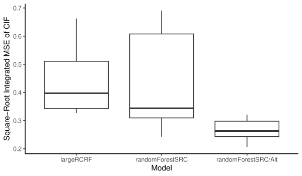
Figure 1: Boxplot of cumulative incidence function (CIF) errors by model. randomForestSRC/Alt is the model produced by randomForestSRC, but tuned using the concordance error as calculated by largeRCRF.

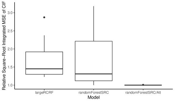
Figure 2: Boxplot of relative cumulative incidence function (CIF) errors by model. For each dataset, all errors are divided by the smallest error produced; values of 1 means that that model produced the lowest error. randomForestSRC/Alt is the model produced by randomForestSRC, but tuned using the concordance error as calculated by largeRCRF.

That said, the next simulation will show that largeRCRF runs significantly faster which could result in better performance if largeRCRF tuned on a denser grid.

3.3 The second simulation - assessing speed

For the timing simulation, we generate 6 datasets; two of size 1000, two of size 10,000, and two of size 100,000. For each pair of datasets we’ll train forests on one and then use that forest to predict on the other, timing how long it takes to train and make predictions for each package, for each size dataset. For both packages we’ll repeat the procedure 10 times for $n=1000$ and 5 times for $n=10,000$. For $n=100,000$ we train largeRCRF 5 times but randomForestSRC only once. The forest parameters used are constant and are:

• Number of splits tried (nsplit): 1000

• Node size (nodeSize): 500

• Number of covariates tried at each split (mtry): 1

	$n=1000$			$n=10,000$			$n=100,000$
Package	Min.	Median	Max.	Min.	Median	Max.	Min.	Median	Max.
largeRCRF	2.10	2.17	2.32	35.7	36.2	37.0	736	742	748
randomForestSRC	7.04	7.14	7.21	3274	3350	3439	-	384061	-

Table 2: The recorded minimum, median, and maximum times (in seconds) recorded for training and predicting for each package for the different sizes of data.

The simulations were run on a desktop computer running Linux with 16GB of RAM and an 8-core 3.5 GHz CPU.

The results, summarized in Table 2, show that largeRCRF is faster than randomForestSRC at all three sizes. At $n=1000$ largeRCRF is only about 3x times faster, but that factor quickly grows as the sample sizes increases. At $n=10,000$ largeRCRF is about 90x faster, and at $n=100,000$ largeRCRF is about 500x faster. This speed increase allows researchers to perform more accurate and denser tuning, especially at larger sample sizes.

4 Examples

We’ll next demonstrate largeRCRF on two real datasets. The first dataset will be a competing risks dataset from The Women’s Interagency HIV Study (wihs) (retrieved from randomForestSRC). This dataset is relatively small at only 1164 rows and 4 possible predictors, making it a small and fast example to demonstrate how to use largeRCRF.

The second dataset is a much larger dataset from an online peer to peer lending company in the United States containing approximately 1.1 million rows and 76 possible predictors, which demonstrates training random competing risks forests on a dataset that was previously too large to work with.

4.1 Women’s Interagency HIV Study

The Women’s Interagency HIV Study (wihs) is a dataset that followed HIV positive women and recorded when one of three possible competing events occurred for each one:

• The woman began treatment for HIV.

• The woman developed AIDS or died.

• The woman was censored for administrative reasons.

There are four different predictors available (age, history of drug injections, race, and a blood count of a type of white blood cells).

The data is included in largeRCRF, but was originally obtained from randomForestSRC. R> data("wihs", package = "largeRCRF") R> names(wihs) [1] "time" "status" "ageatfda" "idu" "black" "cd4nadir"

time and status are two columns in wihs corresponding to the competing risks response, while ageatfda, idu, black, and cd4nadir are the different predictors we wish to train on.

We specify splitFinder = LogRankSplitFinder(1:2, 2), which indicates that we have event codes 1 to 2 to handle, but that we want to focus on optimizing splits for event 2 (which corresponds to when AIDS develops).

We specify that we want a forest of 100 trees (ntree = 100), that we want to try all possible splits when trying to split on a variable (numberOfSplits = 0), that we want to try splitting on two predictors at a time (mtry = 2), and that the terminal nodes should have an average size of at minimum 15 (nodeSize = 15; accomplished by not splitting any nodes with size less than 2 $\times$ nodeSize). randomSeed = 15 specifies a seed so that the results are deterministic; note that largeRCRF generates random numbers separately from R and so is not affected by set.seed().

R> library("largeRCRF") R> model <- + train(CR_Response(status, time)   ageatfda + idu + black + cd4nadir, + data = wihs, splitFinder = LogRankSplitFinder(1:2, 2), + ntree = 100, numberOfSplits = 0, mtry = 2, nodeSize = 15, + randomSeed = 15) Printing model on its own doesn’t do much except print the different components and parameters that made the forest. R> model Call: train.formula(formula = CR_Response(status, time)   ageatfda + idu + black + cd4nadir, data = wihs, splitFinder = LogRankSplitFinder(1:2, 2), ntree = 100, numberOfSplits = 0, mtry = 2, nodeSize = 15, randomSeed = 15)

Parameters: Split Finder: LogRankSplitFinder(events = 1:2, eventsOfFocus = 2) Terminal Node Response Combiner: CR_ResponseCombiner(events = deltas) Forest Response Combiner: CR_FunctionCombiner(events = deltas) # of trees: 100 # of Splits: 0 # of Covariates to try: 2 Node Size: 15 Max Node Depth: 100000 Try using me with predict() or one of the relevant commands to determine error We’ll make predictions on the training data. Since we’re using the training data, largeRCRF will by default only predict each observation using trees where that observation wasn’t included in the bootstrap sample (’out-of-bag’ predictions). R> predictions <- predict(model) Since our data is competing risks data, our responses are several functions which can’t be printed on screen. Instead a message lets us know of several functions which can let us extract the estimate of the survivor curve, the cause-specific cumulative incidence functions, or the cause-specific cumulative hazard functions (CHF). R> predictions[[1]] 2 CIFs available 2 CHFs available An overall survival curve available

See the help page ?CompetingRiskPredictions for a list of relevant functions on how to use this object. Here we extract the cause-specific functions for the AIDS event, as well as the overall survivor curve. R> aids.cifs = extractCIF(predictions, event = 2) R> aids.chfs = extractCHF(predictions, event = 2) R> survivor.curves = extractSurvivorCurve(predictions) Now we plot the functions that we extracted for subject 3; output in Figure 3. R> curve(aids.cifs[[3]](x), from=0, to=8, ylim=c(0,1), + type="S", ylab="CIF(t)", xlab="Time (t)")

R> curve(aids.chfs[[3]](x), from=0, to=8, + type="S", ylab="CHF(t)", xlab="Time (t)")

Figure 3: The out-of-bag estimated AIDS-specific cumulative incidence function (CIF) and cumulative hazard function (CHF) for subject 3.

Finally, we calculate the naive concordance error on the out-of-bag predictions. extractMortalities calculates a measure of mortality by integrating the specified event’s cumulative incidence function from 0 to time, although users are free to substitute their own measures if desired. naiveConcordance then takes the true responses and compares them with the mortality predictions we provide, estimating the proportion of wrong predictions for each event as described by WolbersConcordanceCompetingRisks.

R> mortalities1 <- extractMortalities(predictions, time = 8, event = 1) R> mortalities2 <- extractMortalities(predictions, time = 8, event = 2) R> naiveConcordance(CR_Response(wihs$status,wihs$time), + list(mortalities1, mortalities2)) [1] 0.3939276 0.3535135

We could continue by trying another model to see if we could lower the concordance error, or by integrating the above steps into some tuning algorithm.

4.2 Loan application

When a financial institution makes an installment loan, they may be interested in predicting when a potential borrower will prepay their loan, as this represents a loss of interest income for the financial institution. We have data of approximately 1.1 million three-year loans lent out by an online lender in the United States, containing 76 possible predictors, and the times of loan termination that represent one of:

• How long the loan survived until the borrower defaulted on the loan.

• How long the loan survived until the borrower paid back the loan.

• The loan survived up to a time point (loan is censored due to when data was collected).

We also know for each loan which of the 3 events above occurred. In addition, since we know when the data was collected, we then know the censoring times for every loan, even if it had already terminated.

We would like to use this data to see if it is possible to accurately predict an ’expected loss of interest due to loan prepayment’ that varies enough between borrowers that a financial institution could incorporate the information into their decision models when deciding what, if any, loan terms to offer a prospective borrower.

The response in the dataset includes only the time for when the loan terminated and not any dollar amounts of the prepayment. Thus we are restricted to a competing risks problem. With 76 predictors that have unknown effect on these times and over a million observations, assuming a parametric or semi-parametric model will make poor use of the data with bias dominating any estimates. Thus a non-parametric model like random forests should be considered.

Using largeRCRF, a forest of 100 trees was fit with the following parameters:

• Number of splits tried (nsplit): 1000

• Node size (nodeSize): 10,000

• Number of covariates tried at each split (mtry): 5

We ignored maximum node depth.

This model was trained on a desktop computer with 16GB of RAM and an 8-core 3.5 GHz CPU, which is consumer-level hardware available to most researchers.

First we load the package. Since this is a large dataset we’ll need to explicitly provide much of the system memory by setting the Java parameters. Note that Java’s garbage collector will also need memory, so we ask for a bit beneath 16GB. R> options(java.parameters = c("-Xmx14G", "-Xms14G")) R> library("largeRCRF")

Next we load the data. R> trainingData <- read.csv("trainingData.csv.gz")

Since our interest is only in the repayment event ($\delta=1$) and we have censor times available, we’ll define a GrayLogRankSplitFinder. largeRCRF is designed to support different types of ’split finders’ and ’response combiners’, allowing other researchers to easily add support for other types of random forests using other types of responses without having to re-code the entire random forest algorithm. R> splitFinder <- GrayLogRankSplitFinder(events = 1:2, eventsOfFocus = 1)

Due to how Java and R interface, at some point the data will unfortunately have to be duplicated from R into Java; which is problematic here because of the limited memory. largeRCRF supports deleting the dataset from R’s memory prior to beginning to train the forest, as long as the user provides an R’s environment object containing the data in place of a data frame. R> data.env <- new.env() R> data.env$data<-trainingDataR>rm(trainingData)Finallywecalltrain.Wedon{}^{\prime }tneedtospecifywhichresponsecombinersweuse;largeRCRFcaninferthatbasedonususingcompetingrisksdata.Sincethememoryonthecomputerusedislimitedandthedatasetislargewecanonlyaffordtotrainonetreeatatime,thusthecoresparameterisexplicitlysetto1.Itshouldbenotedthattheothercoresarenotnecessarilyidle;Java{}^{\prime }sgarbagecollectorwillrequirethem,especiallygiventhelimitedmemory.ThesavePathparameterwillhavethepackagesavetreestotheharddriveastheyaresaved,whichwillsavememorywhiletrainingandallowustorecoverourprogressshouldtraininggetinterrupted.R>forest<-+train(CR{}_{R}esponse(delta,u,censorTime).,data.env,+ntree=100,numberOfSplits=1000,mtry=5,nodeSize=10000,+cores=1,splitFinder=splitFinder,savePath=\mathrm{"}saved{}_{f}orest\mathrm{"})Wewanttotrainonalltheavailablepredictors,henceweused.ontheright-handsideoftheformulaasisstandardwhenusingformulaeinR.Trainingthismodeltookabout10.5hours.Nextwereadinourtestdataanduseitforpredictions.R>testData<-read.csv(\mathrm{"}testData.csv.gz\mathrm{"})R>predictions<-predict(forest,testData)AlistofRfunctionsoftheCIFsforrepaymentcanthenbeextractedfromthepredictions.R>cif.predictions<-extractCIF(predictions,1)ApairofloanswithvastlydifferentrepaymentCIFswereselectedsuchthattheysharedthesamedefault-risklevelasprovidedbythefinancialinstitution.Theloansalsowereforthesameloanamount(\$12,000),similarinterestrates(6.97\%,7.21\%),andsimilarmonthlyloanpayments(\$370.37,\$371.68).WeplotthesecurvestogetherasshowninFigure\text{<a href="\#S4.F4" title="Figure 4 ‣ 4.2 Loan application ‣ 4 Examples ‣ Random Competing Risks Forests for Large Data" class="ltx\_ref ltx\_font\_italic"><span class="ltx\_text ltx\_ref\_tag">4</span></a>}.R>pred{}_{l}ow<-cif.predictions[[20718]]R>pred{}_{h}igh<-cif.predictions[[3073]]R>curve(pred{}_{h}igh(x),from=0,to=36,type={}^{\prime }S{}^{\prime },col={}^{\prime }blue{}^{\prime },+ylab=\mathrm{"}CIF-Payoff(t)\mathrm{"},xlab=\mathrm{"}Time(Months)\mathrm{"})R>curve(pred{}_{l}ow(x),from=0,to=36,type=\mathrm{"}S\mathrm{"},col={}^{\prime }red{}^{\prime },+add=TRUE)R>legend(x=1,y=0.8,legend=c(\mathrm{"}High\mathrm{"},\mathrm{"}Low\mathrm{"}),+col=c(\mathrm{"}blue\mathrm{"},\mathrm{"}red\mathrm{"}),lty=1)\text{Figure 4Figure 44Figure 44Plotofthepredictedrepaymentcumulativeincidencefunctions(CIF}$